Simulation-Based Two-Stage Machine Learning Approach for Fault Detection and Severity Estimation in Industrial Gas Turbines

Abstract

Heavy-duty industrial gas turbines accumulate performance degradation in the compressor and turbine sections during continuous operation, making reliable fault diagnosis essential for safe and efficient operation. This study presents a two-stage machine learning framework for fault detection and severity estimation, developed and evaluated on a single-shaft gas turbine model inspired by the GE 7HA.03. A damage propagation model, adapted from an established NASA methodology, simulated compressor fouling, turbine erosion, and their combined occurrence across three load conditions, generating 34,560 training and 2880 testing samples via Monte Carlo sampling of ambient conditions and multiplicative Gaussian noise injection. The first stage employs a calibrated, selective XGBoost classifier that withholds low-confidence predictions for manual review, achieving 98.6% classification accuracy at 94.7% coverage. The second stage uses a Multi-Task Learning multilayer perceptron with dedicated output heads for compressor and turbine degradation, achieving an aggregate R² above 0.985 and a mean absolute error below 0.156 percentage points. Explainability analysis via SHAP and permutation importance confirmed that both stages rely on physically interpretable sensor signals. Finally, robustness testing across interpolated severity levels and elevated sensor noise defined the system’s operational boundaries, supporting its applicability to industrial condition monitoring.

1. Introduction

Industrial gas turbines operating in continuous power-generation service accumulate performance degradation gradually across their compressor and turbine sections. Left undetected, this degradation reduces thermal efficiency and output capacity, accelerates mechanical deterioration, and increases the risk of unscheduled outages. Reliable, continuous fault diagnosis is therefore essential for safe and economically efficient operation.

Degradation in industrial gas turbines arises through several distinct physical mechanisms, including fouling, erosion, corrosion, and tip clearance increase, each differing in onset rate, reversibility, and detectability from gas path measurements [1]. Compressor Fouling (CF) is the most operationally prevalent of these mechanisms: airborne particulate matter and humidity-borne deposits accumulate on blade surfaces, altering blade profile geometry and reducing both isentropic efficiency and flow capacity [2]. Fouling progresses continuously during operation and typically accounts for the largest share of recoverable performance losses in land-based gas turbines [3]. Turbine Erosion (TE) presents a distinct signature: hard particles passing through the hot section abrade blade leading edges and tip regions, widening clearances and degrading turbine flow capacity in a manner that is largely irreversible without hardware replacement [2]. Because both mechanisms produce thermodynamically measurable, parametrically modellable deviations and represent the dominant sources of performance loss in heavy-duty industrial gas turbines [4], this study targets CF and TE, individually and in simultaneous combination (Double Fault, DF), as the diagnostic classes of interest.

In the diagnostic part, data-driven fault classification of gas turbines has been studied extensively over the past decade, progressively displacing model-based approaches such as Gas Path Analysis [5], and the reported classification accuracies are generally high [6]. Using K-Nearest Neighbors, Neural Network, and Decision Tree classifiers, fault detection and isolation accuracies of up to 99% have been reported across six single- and six double-component fault classes in a three-shaft industrial gas turbine [7], while an artificial neural network achieved 94.55% classification accuracy for CF, TE, and their simultaneous occurrence in a hydrogen-fueled micro gas turbine, outperforming support vector machine, decision tree, random forest, and k-nearest neighbor baselines [8]. A combined Kalman filter–ANN–fuzzy logic framework applied to a two-spool industrial gas turbine has similarly reported classification accuracies above 95% and quantification accuracies above 92% for compressor fouling, turbine fouling, and turbine erosion under randomized deterioration magnitude and nominal measurement noise [9].

However, standard classifiers commit to a prediction for every input regardless of whether that input lies within the distribution of the training data—a behavior with direct operational consequences, since predictions on boundary-condition or degraded-sensor inputs carry no indication of their own reliability. Selective classification, in which a classifier abstains from prediction below a defined confidence threshold, addresses this limitation and has been formalized for neural networks—for example, through the coverage–accuracy trade-off framework of SelectiveNet, presented by Geifman et al. [10]. However, applications of confidence-aware classification to gas turbine diagnostics remain sparse: existing approaches [11,12] use post hoc confidence measures derived from model architecture rather than calibrated probability estimates tied to an explicit coverage target. A formally calibrated selective classification system, with a threshold selected to achieve a defined coverage–accuracy operating point, has no direct precedent in the gas turbine fault diagnosis literature.

A second related gap concerns fault quantification. Neural network approaches have been used to recover degradation magnitude from gas path measurements [4,9,13], but existing architectures treat the health parameters of different components as homogeneous outputs of a single network layer, without exploiting the structural separation between compressor-side and turbine-side degradation. Multi-Task Learning (MTL), in which a shared representation feeds task-specific output heads, offers a more structured alternative and has been applied to simultaneous fault detection and severity estimation in rotating machinery more broadly [14,15]. However, its application to gas path health-parameter regression, where compressor and turbine degradation form a natural task partition, has not been reported.

This study addresses both gaps through a unified two-stage diagnostic framework applied to a single-shaft heavy-duty gas turbine model. Rather than treating an uncertain prediction as a failure to be concealed, the framework treats it as diagnostically informative in its own right: a system that is permitted to withhold judgment, to say it does not know, is more trustworthy than one forced to commit to a label regardless of the evidence, a property that matters most precisely in the safety-critical setting this work addresses.

2. Methodology Overview

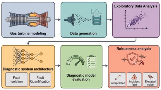
A six-phase pipeline structures the methodology developed here, summarised in Figure 1, with each phase building on the previous one. A validated thermodynamic simulation of the reference gas turbine first supplies the basis for a synthetic dataset, generated through a damage propagation model under Monte Carlo-sampled ambient conditions and realistic sensor noise. Exploratory analysis of this dataset then informs the design of a two-stage diagnostic system: a selective classifier for fault isolation, followed by a multi-task regressor for fault quantification. The resulting pipeline is evaluated end-to-end, and finally stress-tested for robustness under interpolated, near-threshold, and elevated-noise conditions to establish its practical operating envelope.

Figure 1. Methodological flowchart of the study.

3. Simulation Model and Dataset Generation

3.1. Gas Turbine Simulation Model

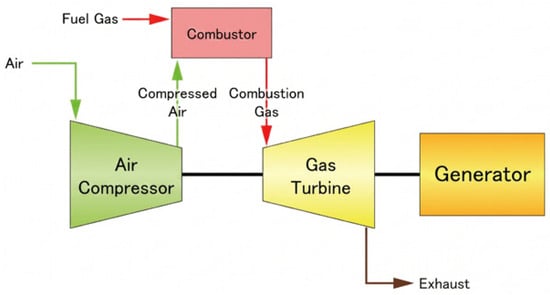
The reference engine adopted in this study is a single-shaft industrial gas turbine inspired by the natural-gas-fired General Electric (GE Vernova, Cambridge, MA, USA) 7HA.03, the latest model in the 7HA series. It operates on a simple Brayton cycle at a constant rotational speed of 3600 rpm (60 Hz), featuring a 14-stage compressor and a 4-stage turbine [16]. Figure 2 illustrates the general layout adopted.

Figure 2. Single-shaft industrial gas turbine architecture. Source: Wikipedia Commons.

The design point matching procedure targeted the manufacturer’s published net shaft power (430 MW) and net thermal efficiency (43.3%) at ISO conditions (288 K, 1.013 bar, 60% RH) [16]. Five unknown component parameters were estimated through an inverse, literature-informed matching procedure, following the approach of Li et al. [17] for engines with limited public data, converging to a compressor pressure ratio of 24.3, a turbine entry temperature of 1923 K, an inlet mass flow of 682 kg/s, and compressor and turbine isentropic efficiencies of 0.91 each, all consistent with published H-class ranges [17].

Convergence was evaluated using the Relative Percentage Error (RPE) between the simulated and target values for net shaft power and net thermal efficiency:

$$\mathit{RPE}= \left|{\displaystyle \frac{X_{\mathit{sim}}-X_{\mathit{target}}}{X_{\mathit{target}}}}\right|\times 100\%$$

where Xsim is the value obtained from the simulation model and Xtarget the corresponding value published by the manufacturer, with convergence accepted when RPE ≤ 0.1% for both quantities, consistent with comparable design-point matching studies in the literature [18]. As reported in Table 1, the matched model achieved RPE values of 0.10% for net shaft power and 0.07% for net thermal efficiency, confirming a successful design-point match and establishing the validated baseline model used for all subsequent degradation simulations.

Table 1. RPE calculations for the simulated outputs.

Outputs	Targets (GE Vernova)	Simulated	RPE
Net Shaft Power (MW)	430.0	429.560	0.10%
Net Thermal Efficiency (%)	43.3	43.27	0.07%

3.2. Damage Propagation Model

Industrial gas turbines operating at a constant duty cycle accumulate performance degradation gradually over their service life. Following a physics-inspired approach, wear is assumed to evolve exponentially, and the engine’s health state can be expressed as a function of time:

$$h\left(t\right)=1-\mathit{exp}(a{t}^b)$$

(1)

where h(t) is the health parameter loss at operating time t, a is the scale parameter, and b is the shape parameter, consistent with the damage propagation framework of Saxena et al. [19]. This formulation captures macro-level degradation trends while abstracting away micro-level physical processes. This formulation was separated into independent efficiency and flow-capacity components for the compressor and turbine (Equation (2)), with the shape parameter b set to 1.5 following Saxena et al. [19].

$$\left\{\begin{array}{c}e\left(\tau \right)=1-\exp \left(a_e{\tau }^{b_e}\right)\\ f\left(\tau \right)=1-\exp \left(a_f{\tau }^{b_f}\right)\end{array}\right.$$

(2)

The scale parameter a for each component was calibrated using published degradation rates at the 50,000-h major overhaul interval characteristic of heavy-duty gas turbines such as the GE 7HA [20]: a 5% efficiency and 6% flow-capacity reduction for severe compressor fouling [21], and a 2.5% efficiency reduction with a 2% flow-capacity increase under heavy turbine erosion [22]. The resulting calibrated constants are calculated, yielding the final component-specific degradation equations (Equations (3) and (4)) used to generate degradation profiles at ten equally spaced normalized time points, from initial operation (τ = 0.1) to major overhaul (τ = 1), as summarized in Table 2.

$$\left\{\begin{array}{c}e\left(\tau \right)=1-\exp \left(-0.051293 {\tau }^{1.5}\right)\\ f\left(\tau \right)=1-\exp \left(-0.061875 {\tau }^{1.5}\right)\end{array}\right.$$

(3)

$$\left\{\begin{array}{c}e\left(\tau \right)=1-\exp \left(-0.025318 {\tau }^{1.5}\right)\\ f\left(\tau \right)=1-\exp \left(0.019803 {\tau }^{1.5}\right)\end{array}\right.$$

(4)

Table 2. Calculated degradation levels.

		Degradation Levels
		Level 1	Level 2	Level 3	Level 4	Level 5	Level 6	Level 7	Level 8	Level 9	Level 10
Compressor Fouling	Δnc	−0.16%	−0.46%	−0.84%	−1.29%	−1.80%	−2.36%	−2.96%	−3.60%	−4.28%	−5.00%
	ΔΓc	−0.20%	−0.55%	−1.01%	−1.55%	−2.16%	−2.83%	−3.56%	−4.33%	−5.15%	−6.00%
Turbine Erosion	Δnt	−0.08%	−0.23%	−0.42%	−0.64%	−0.89%	−1.17%	−1.47%	−1.80%	−2.14%	−2.50%
	ΔΓt	0.06%	0.18%	0.33%	0.50%	0.70%	0.92%	1.17%	1.43%	1.71%	2.00%

Equations (1)–(4) express the fractional loss of each health parameter, so a positive value denotes a reduction; Table 2 reports the same levels with the sign convention of the engine simulation deck, in which deterioration is entered as a signed change relative to the healthy component (negative for a reduction, positive for an increase), so that each tabulated value equals −e(τ) or −f(τ). The turbine erosion flow capacity therefore appears to be a positive change, reflecting the increase in effective flow area of an eroded turbine.

Degradation levels 1 and 2 were excluded from the single-fault classes, following Fentaye et al. [4], since their thermodynamic deviations fall within the sensor measurement uncertainty band and would otherwise inflate false-alarm risk.

3.3. Data Generation Process

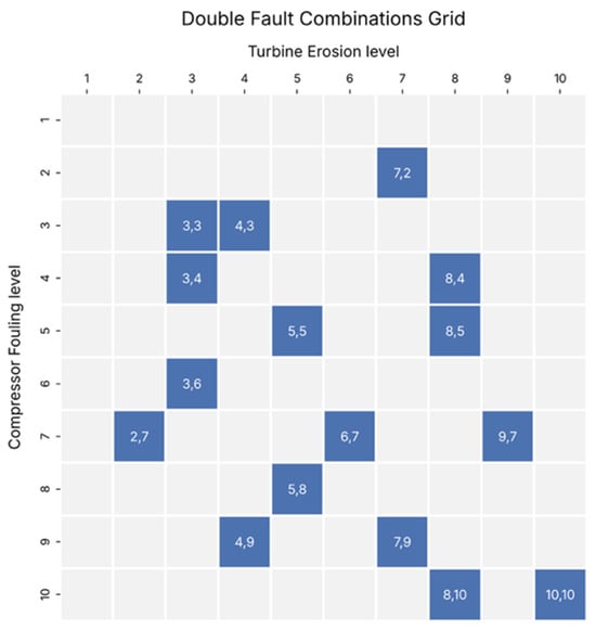
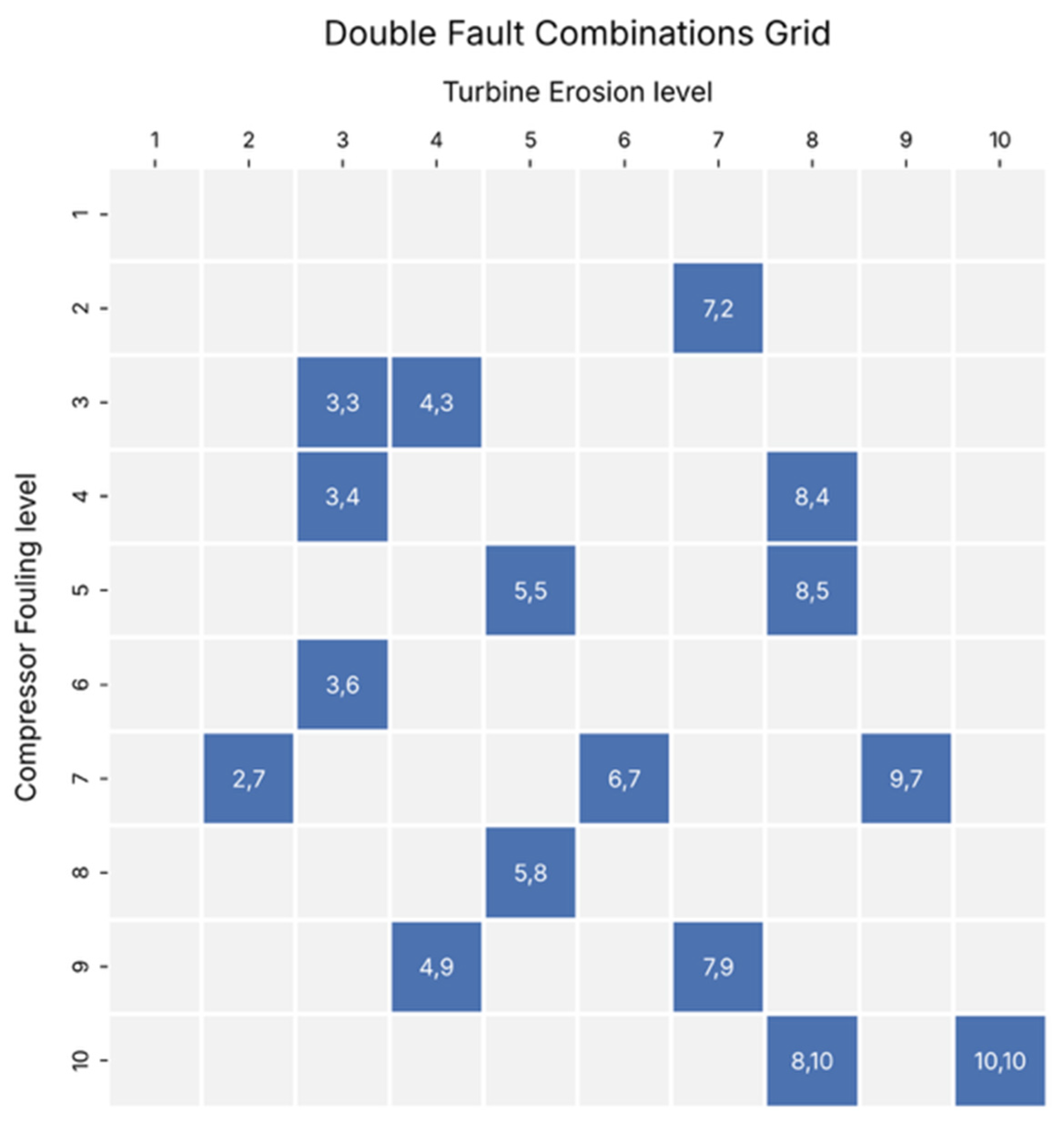
To capture realistic operating variability, ambient temperature (0–40 °C) and relative humidity (20–90%) were treated as stochastic inputs sampled from uniform distributions via the engine simulation deck off-design Monte Carlo simulation tool, rather than simulating performance at fixed discrete points. Rotational speed was fixed at 3600 rpm to reflect grid-synchronized operation, and a turbine entry temperature limiter was applied at the design-point value (1923 K) to reflect realistic controller behavior under high ambient temperature or severe degradation. The engine was simulated across three discrete load conditions (50%, 75%, and 100% of rated power), each encoded as one-hot load indicators, across all four health states (Healthy, CF, TE, DF). The discrete representation was adopted to keep the simulation campaign tractable, since each additional load point multiplies the number of required runs across all health states and severity levels. Consequently, the trained models are defined only at these three load points. For the Double Fault class, mapping the full two-dimensional space of compressor–turbine severity combinations would have required a prohibitively large number of simulations: with eight severity levels per component, the complete grid comprises 64 combinations per load condition. Instead, 16 combinations per load condition were selected under three criteria. First, every CF and every TE severity level from 3 to 10 appears at least once, so that each marginal severity is represented in the training data. Second, the combinations are distributed over both the diagonal of the severity plane, where the two components are degraded to a similar extent, and their off-diagonal regions, where one fault dominates, so that no quadrant of the plane is left unsampled. Third, two combinations deliberately pair a sub-threshold level (2) in one component with a severe level (7) in the other, to cover the boundary between the Double Fault and single-fault classes: although Level 2 alone falls within the sensor noise floor and is excluded from the single-fault classes, its co-occurrence with a Level 7 fault in the other component produces a joint thermodynamic deviation that remains diagnostically significant. The selected combinations are listed in Figure 3.

Figure 3. Simulated combination grid for the Double Fault class.

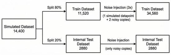
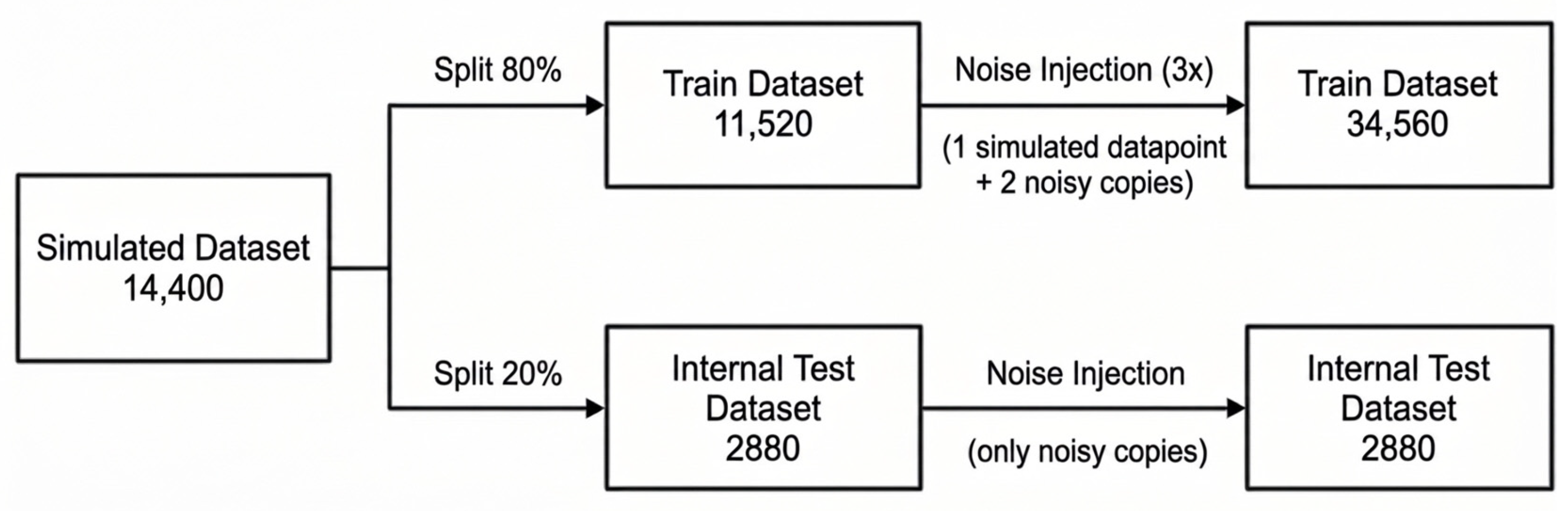
Each simulation run yielded nine gas path sensor signals as output, summarized in Table 3. Aggregating across all combinations of health state, severity level, and load condition produced an initial dataset of 14,400 data points, balanced by design across the four health classes (3600 points per class) and the three load conditions (4800 points per load). This dataset was subsequently partitioned into training and internal test sets via a stratified 80/20 split, preserving both class and load ratios.

Table 3. Extracted sensor signals to be used as inputs for the diagnostic model.

Symbols	Descriptions	Units
T1	Ambient Temperature	K
RH	Relative Humidity	%
W2	Engine Mass Flow	kg/s
T3	Compressor Discharge Temperature	K
P3	Compressor Discharge Pressure	kPa
WF	Burner Fuel Flow	kg/s
T5	Turbine Discharge Temperature	K
P5	Turbine Discharge Pressure	kPa
Psh	Shaft Power Delivered	kW

Furthermore, to simulate realistic measurement uncertainty, Multiplicative Gaussian Noise (MGN) was applied to all sensor channels, scaling noise intensity with signal magnitude to reflect the behavior of physical instrumentation:

$$y_{\mathit{noisy}}= y_{\mathit{clean}}·\left(1+n_i\right), n_i ~ N\left(0, {\left({\displaystyle \frac{u_i}{3}}\right)}^2\right)$$

where y_clean is the simulated sensor value, y_noisy is the corresponding noisy measurement, n_i is a zero-mean Gaussian random variable drawn independently for each sample, and u_i denotes the published instrument uncertainty of sensor i, treated as a 3σ (99.7% confidence) bound consistent with Type B evaluation under the ISO GUM standard [23]. Sensor-specific uncertainty values and their literature sources are listed in Table 4.

Table 4. Sensors uncertainty levels.

Sensors	Uncertainties	References
T1, T3, T5	±0.4%	[24]
P3, P5	±0.2%	[25]
WF	±0.5%	[26]
Psh	±0.1%	[27]
W2	±0.5%	[28]
RH	±2.0%	[26]

Noise was applied asymmetrically across partitions, as shown in Figure 4: each training sample was augmented with two independent noise copies to improve model robustness, while each test sample received a single noise realization to emulate a realistic field measurement. This yielded a final training set of 34,560 data points and an internal test set of 2880 data points, both maintaining exact class balance across the four health states. The final feature matrix comprises nine sensor-derived inputs and three one-hot load indicators, for a total of twelve input features per sample.

Figure 4. Data handling flowchart from simulations to noise injection.

4. Exploratory Data Analysis

Before model development, an Exploratory Data Analysis (EDA) verified the physical consistency of the simulated sensor data, quantified sensor-to-fault dependence, and assessed the geometric complexity of the classification problem.

4.1. Correlation Structure

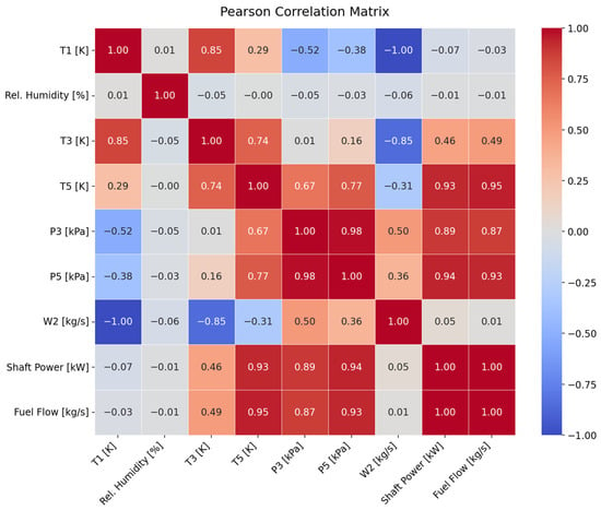
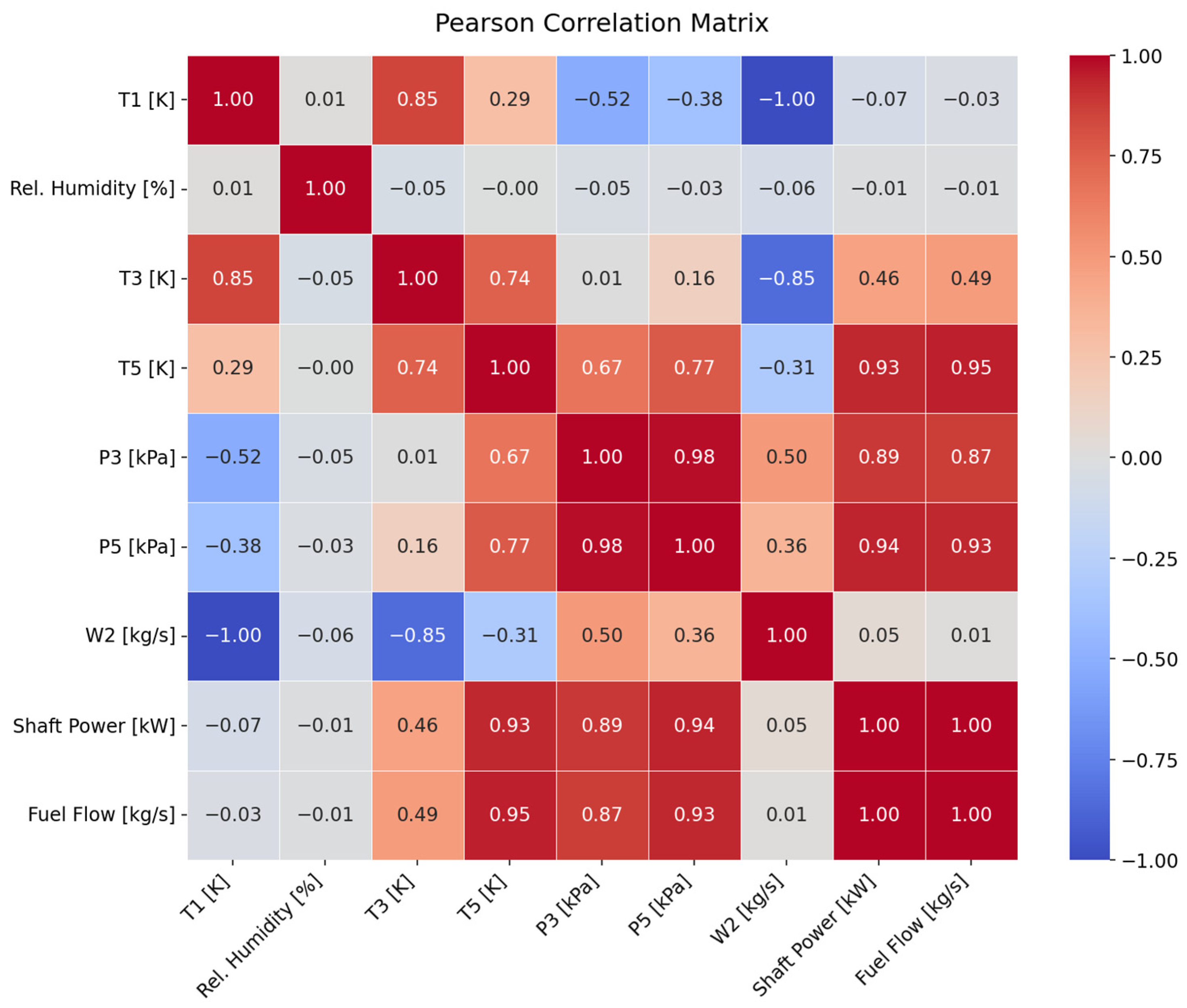
A Pearson correlation matrix computed over the Healthy-class subset across all three load conditions (Figure 5) reproduced known Brayton-cycle couplings: shaft power and fuel flow showed a perfect positive correlation (r = 1.00), consistent with the combustion energy balance. Both correlated strongly with turbine exit temperature and compressor/turbine exit pressures (r = 0.87–0.95). Ambient temperature showed a near-perfect negative correlation with engine mass flow (r = −1.00), reflecting the corrected-flow relationship, while relative humidity showed negligible correlation with all gas path sensors. This confirms that the simulated dataset respects the underlying thermodynamic coupling of the cycle and identifies a multicollinearity structure—notably among turbine exit temperature, compressor/turbine exit pressures, shaft power, and fuel flow—that later motivates the nonlinear, redundancy-tolerant feature treatment adopted in the diagnostic pipeline.

Figure 5. Pearson correlation matrix for all nine sensor channels.

4.2. Mutual Information Analysis

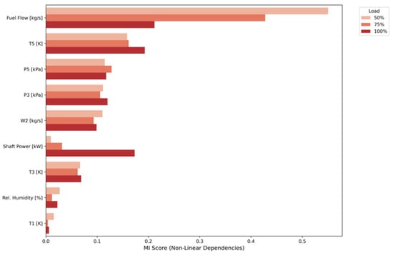
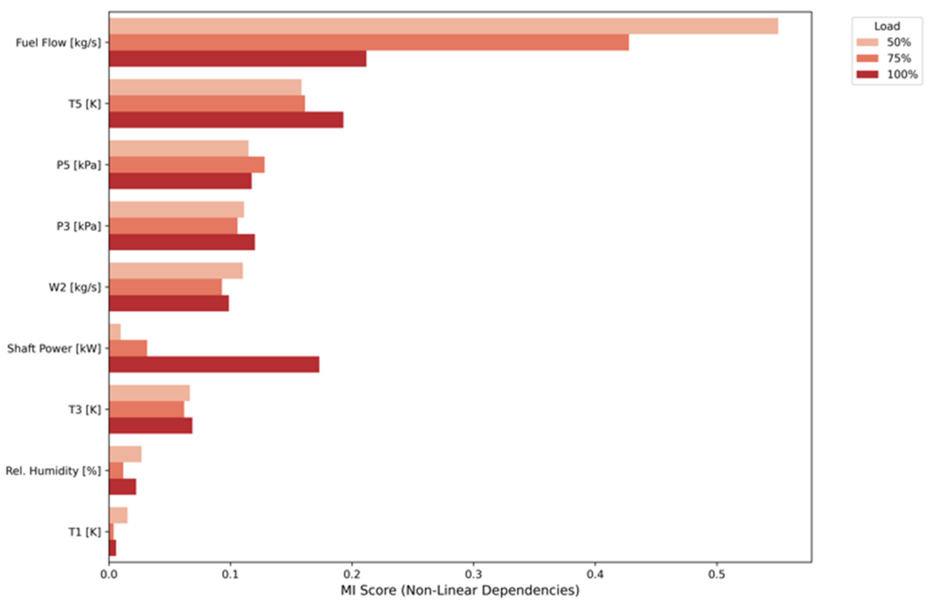
Mutual Information (MI) between each sensor and the fault class label, computed separately within each load condition to prevent load-induced variance from inflating apparent discriminability (Figure 6), identified fuel flow as the most informative channel at 50% and 75% load, though no single sensor dominated across all three load conditions simultaneously. This distributed pattern indicates that fault-discriminative information is spread across multiple sensor channels in a load-dependent manner, motivating full-feature retention in the diagnostic model rather than aggressive dimensionality reduction.

Figure 6. MI scores per sensor representation across all three load conditions.

4.3. Class Separability

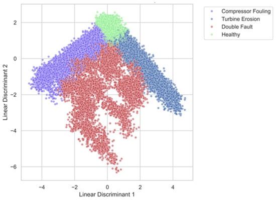
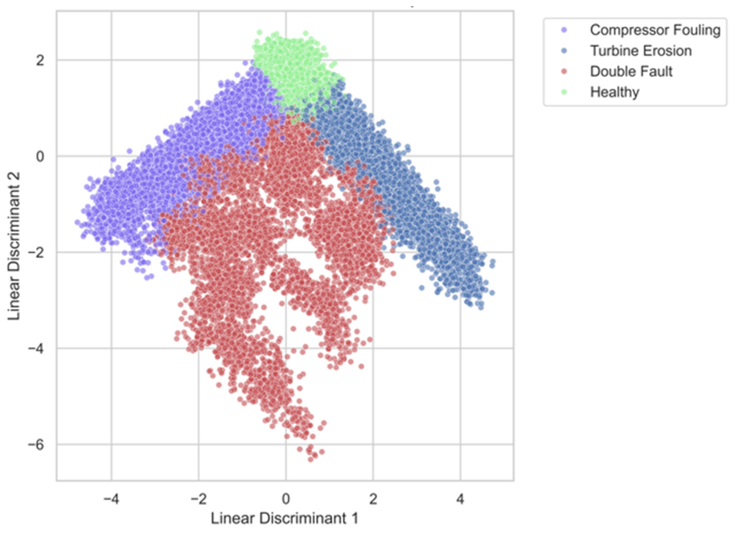
Linear Discriminant Analysis (LDA)—a supervised projection maximizing between-class separation relative to within-class spread—was applied to assess whether the classification problem admits a linear decision boundary. Figure 7 illustrates that the Healthy class occupied a compact, well-separated region of the discriminant space, while the three fault classes overlapped substantially; DF in particular spread across a broad, diffuse region encroaching on both single-fault classes, consistent with a signature that combines elements of both individual faults in proportions that vary with relative component severity. Because this overlap persisted even under the optimal linear projection, the fault classes are not linearly separable, directly motivating the nonlinear ensemble methods adopted for Stage 1 of the diagnostic pipeline.

Figure 7. LDA projection colored by health state.

Together, these three analyses establish that the simulated dataset is physically valid, that fault signatures are detectable but distributed across sensor channels in a load-dependent way, and that the classification problem requires nonlinear decision boundaries—jointly justifying the architectural choices developed in Section 5.

5. Two-Stage Diagnostic Framework Development

5.1. Concept & Rationale

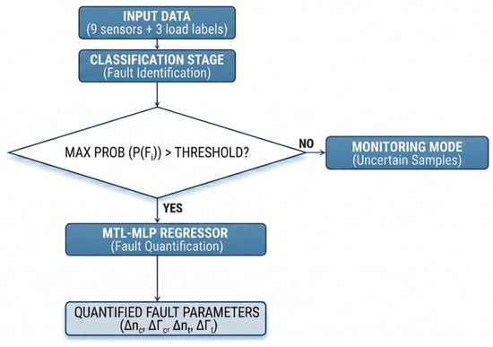
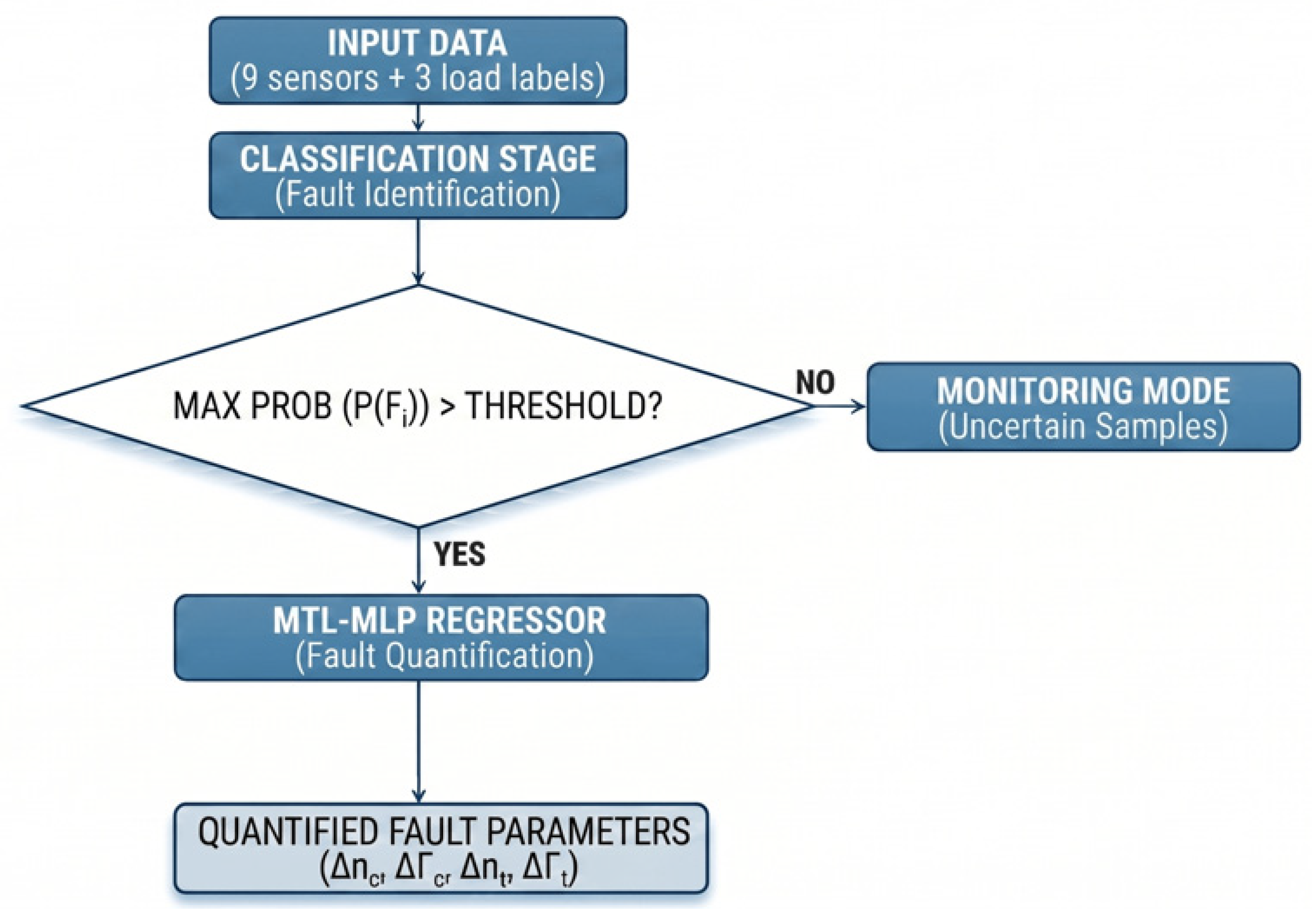
The diagnostic framework developed in this study adopts a two-stage sequential architecture that combines fault identification with fault severity quantification, organized around the principle of selective classification: rather than forcing a decision on every input sample, the system withholds judgment whenever classifier confidence falls below a defined threshold, routing those samples to a separate monitoring channel instead of a forced label.

In Stage 1, a calibrated classifier receives a twelve-dimensional input vector and outputs a probability distribution over four health states. Raw classifier scores are first calibrated via isotonic regression; the maximum calibrated class probability, max P(Fi), is then compared against a confidence threshold θ. Samples satisfying max P(Fi) ≥ θ are accepted as confident predictions and passed to Stage 2, while samples falling below θ are redirected to a Monitoring Mode, flagged for review by a field engineer rather than assigned a forced diagnostic label. In Stage 2, samples classified as faulty with sufficient confidence are passed to a MTL-Multilayer Perceptron (MLP) regressor, which estimates up to four degradation parameters depending on the identified fault type. Healthy samples are excluded from this stage, since degradation quantification is not physically meaningful for them. Figure 8 illustrates the complete conceptual pipeline.

Figure 8. Flowchart of the conceptual pipeline.

This architecture is motivated by two considerations. First, the selective classification mechanism mirrors the operating logic of safety-critical industrial systems, where ambiguous or borderline sensor readings should trigger an alert rather than an automated, potentially incorrect diagnosis—a misclassification propagated into the regression stage would otherwise produce degradation estimates with no physical correspondence, risking misleading maintenance decisions. Second, decoupling fault identification from severity estimation keeps the two stages as independently trainable components: each can be optimized, evaluated, and replaced without affecting the other, making the diagnostic logic more transparent to the engineer reviewing flagged cases.

5.2. Stage 1: Selective Classification

5.2.1. Candidate Algorithms and Threshold Selection

The Stage 1 classifier must produce per-sample probability estimates suitable for confidence-based thresholding. This requirement directed the search toward the ensemble tree-based family—Random Forest (RF), XGBoost, LightGBM, and CatBoost—for three reasons: these methods derive class probabilities directly from the vote distribution across constituent trees and are therefore inherently probabilistic; they are resilient to multicollinearity among input features; and their non-parametric decision boundaries can capture the nonlinear fault signatures identified in Section 4.3, without requiring explicit feature transformation. Because raw tree-ensemble probability outputs are not statistically calibrated, isotonic regression calibration was applied to all four classifiers after hyperparameter tuning, using a held-out 20% validation split drawn from the training data. Isotonic regression was preferred over Platt scaling, since it imposes no parametric (sigmoidal) assumption on the score-to-probability mapping—a property better suited to the irregular score distributions typical of tree ensembles.

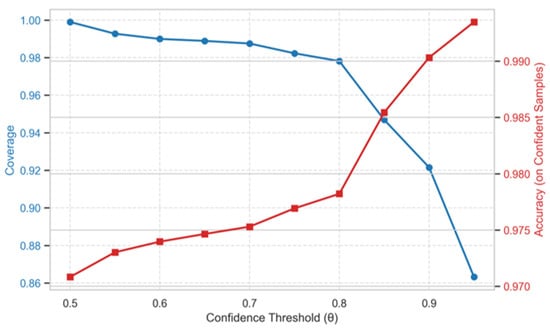
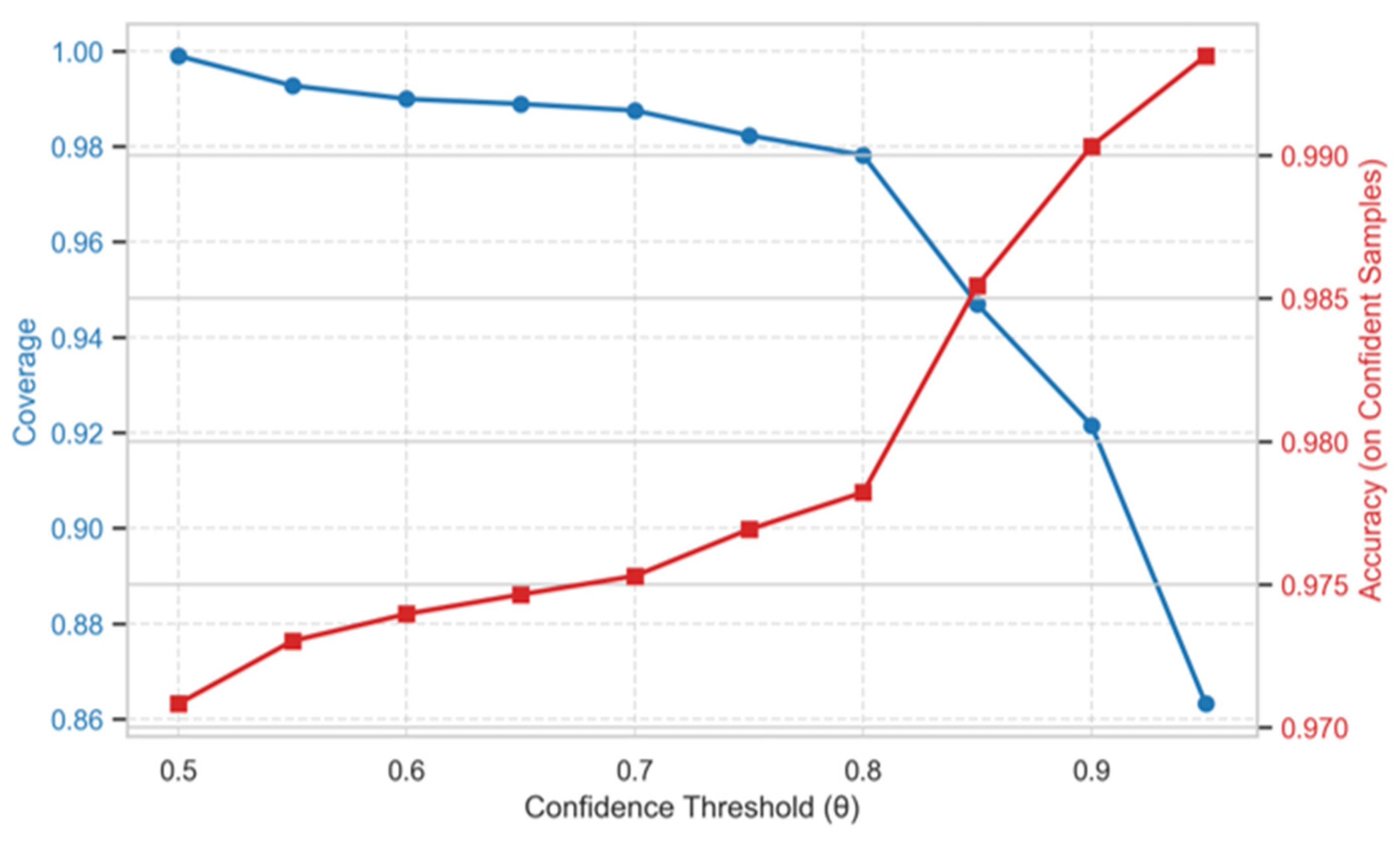
The confidence threshold θ governs the boundary between confident predictions, which proceed through the pipeline, and uncertain samples, which are routed to Monitoring Mode. Coverage and balanced accuracy on the accepted subset were evaluated for each calibrated classifier across θ ∈ [0.50, 0.95] in increments of 0.05, using the internal test set. Figure 9 shows the clearest inflection structure among the four algorithms: coverage declines gradually from 1.00 to 0.98 as accuracy rises from 0.864 to 0.978 between θ = 0.50 and θ = 0.80, before entering a steeper coverage decline beyond θ = 0.85 (the “knee” of the curve) and a region of diminishing accuracy returns beyond θ = 0.90. A common operating threshold of θ = 0.85 was selected for all four classifiers, based on the knee-point criterion and on cross-algorithm consistency—at this value, all four classifiers exhibit a measurable, operationally meaningful abstention rate.

Figure 9. Coverage and accuracy trends for different confidence thresholds for the XGBoost classifier.

5.2.2. Algorithm Selection

Final algorithm selection was based on four criteria, evaluated in sequence: cross-validated (CV) training performance as an independent screening measure, followed by threshold-based coverage at θ = 0.85, classification accuracy on the confident subset, and total misclassified samples among accepted predictions—the latter three used jointly to distinguish among the closely performing candidates. Table 5 summarizes all four criteria across the candidate algorithms.

Table 5. Candidate algorithm comparison across all four selection criteria.

Algorithms	CV Accuracy ± Std (%)	Coverage (%)	Test Accuracy (%)	Misclassified Samples (%)
Random Forest	96.66% ± 0.0038	90.4	97.7	2.3
XGBoost	98.23% ± 0.0024	94.7	98.6	1.4
LightGBM	98.45% ± 0.0025	96.0	98.1	1.9
CatBoost	96.74% ± 0.0025	91.7	98.6	1.3

XGBoost and LightGBM achieved the highest CV accuracy, outperforming Random Forest and CatBoost by 1.5–1.8 percentage points, with uniformly low fold-to-fold variance (<0.004%) indicating stable generalization. At θ = 0.85, LightGBM’s coverage (96.0%) fell outside the 5–7% abstention range identified as operationally desirable for industrial monitoring, indicating that its probability mass was concentrated near the score-distribution boundaries and the abstention mechanism was only partially active at this threshold. XGBoost and CatBoost tied for the highest test accuracy (98.6%); however, CatBoost’s marginally lower total misclassification count reflects its lower coverage rather than superior discrimination. Across all algorithms, the DF class accounted for the largest share of misclassifications, consistent with the class-overlap pattern identified via LDA.

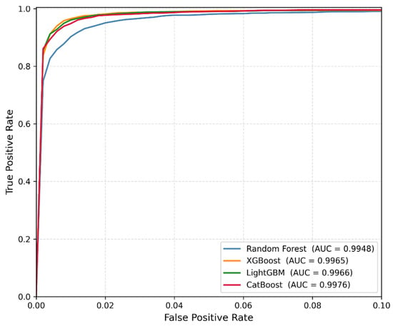
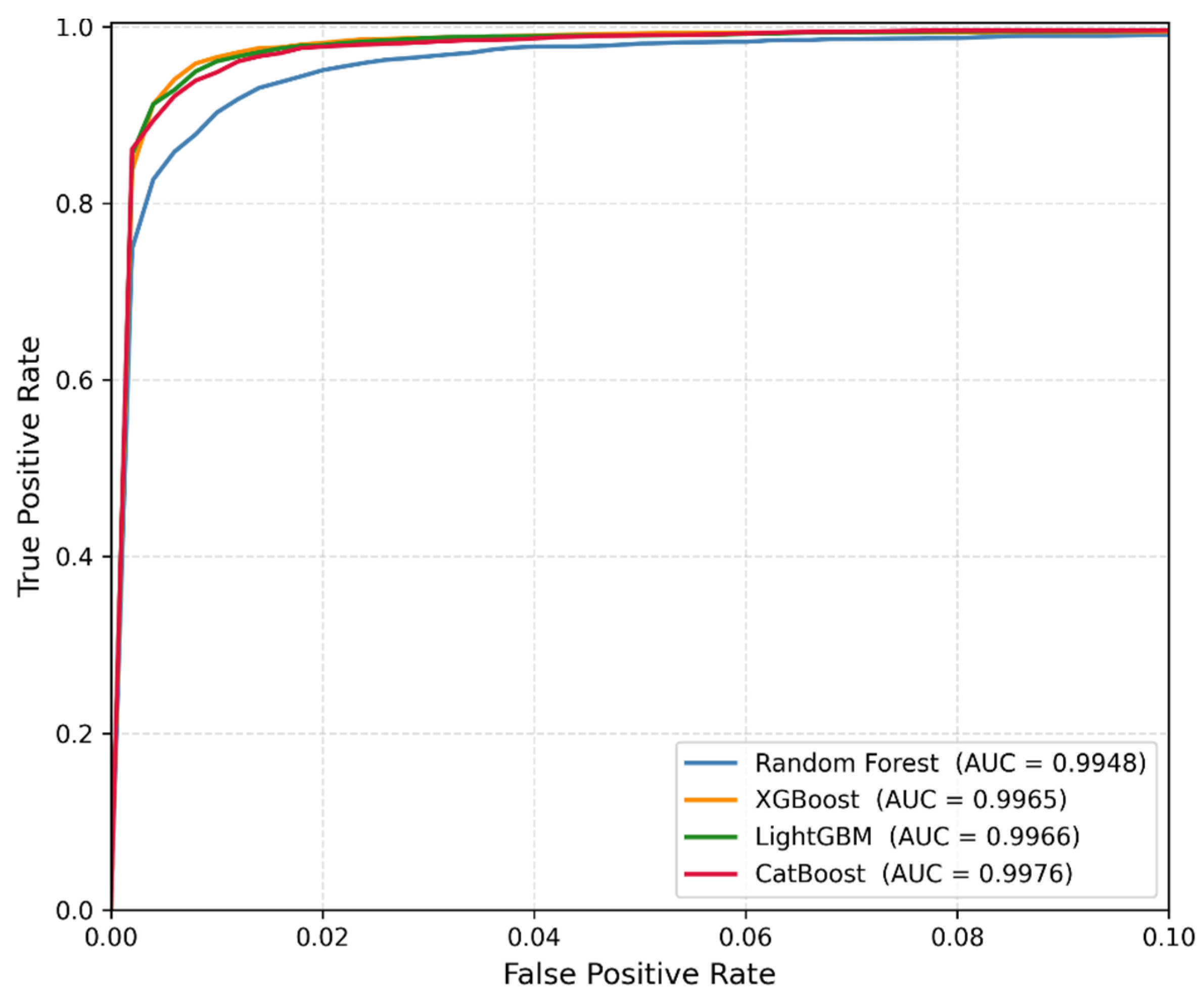
As a final, threshold-independent confirmation, the macro-average Receiver Operating Characteristic (ROC) curves for all four classifiers, as shown in Figure 10, support this ranking: all four classifiers achieved AUC values above 0.994, with Random Forest showing the earliest deviation from the ideal point in the low-false-positive-rate region—consistent with its lower cross-validated accuracy—while XGBoost, LightGBM, and CatBoost remained tightly clustered near the top-left corner.

Figure 10. Macro-average ROC curves for all four classifiers.

Taken together, XGBoost offered the most balanced profile across all four criteria—high cross-validated accuracy, an operationally appropriate abstention rate, test accuracy tied for highest, and a low misclassification count relative to its coverage—and was therefore selected as the Stage 1 classifier.

5.3. Stage 2: MTL-MLP Regressor Architecture

Multi-Task Learning, a paradigm in which a single model predicts multiple outputs by sharing internal representations across tasks rather than fitting independent models to each [14], was adopted because the four degradation parameters estimated in Stage 2 are physically coupled: jointly determined by the same gas-path thermodynamic state and measured by the same sensor set, such that estimating them independently would discard this structure. A hard-parameter-sharing configuration was selected specifically because it allows this physical organization to be encoded directly in the network topology: a shared trunk learns a common gas-path representation, from which two task-specific heads—one for compressor parameters, one for turbine parameters—decode outputs, mirroring the underlying component-level separation of the fault domains.

Input features were standardized using a scaler fitted on the training partition only; the four regression targets were standardized independently via a separate scaler fitted on the training targets, preventing the larger-magnitude compressor outputs from dominating the Mean Squared Error (MSE) loss and suppressing gradient updates for the smaller-magnitude turbine outputs. All predictions were inverse-transformed prior to metric computation to recover estimates in their original percentage units.

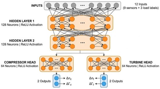
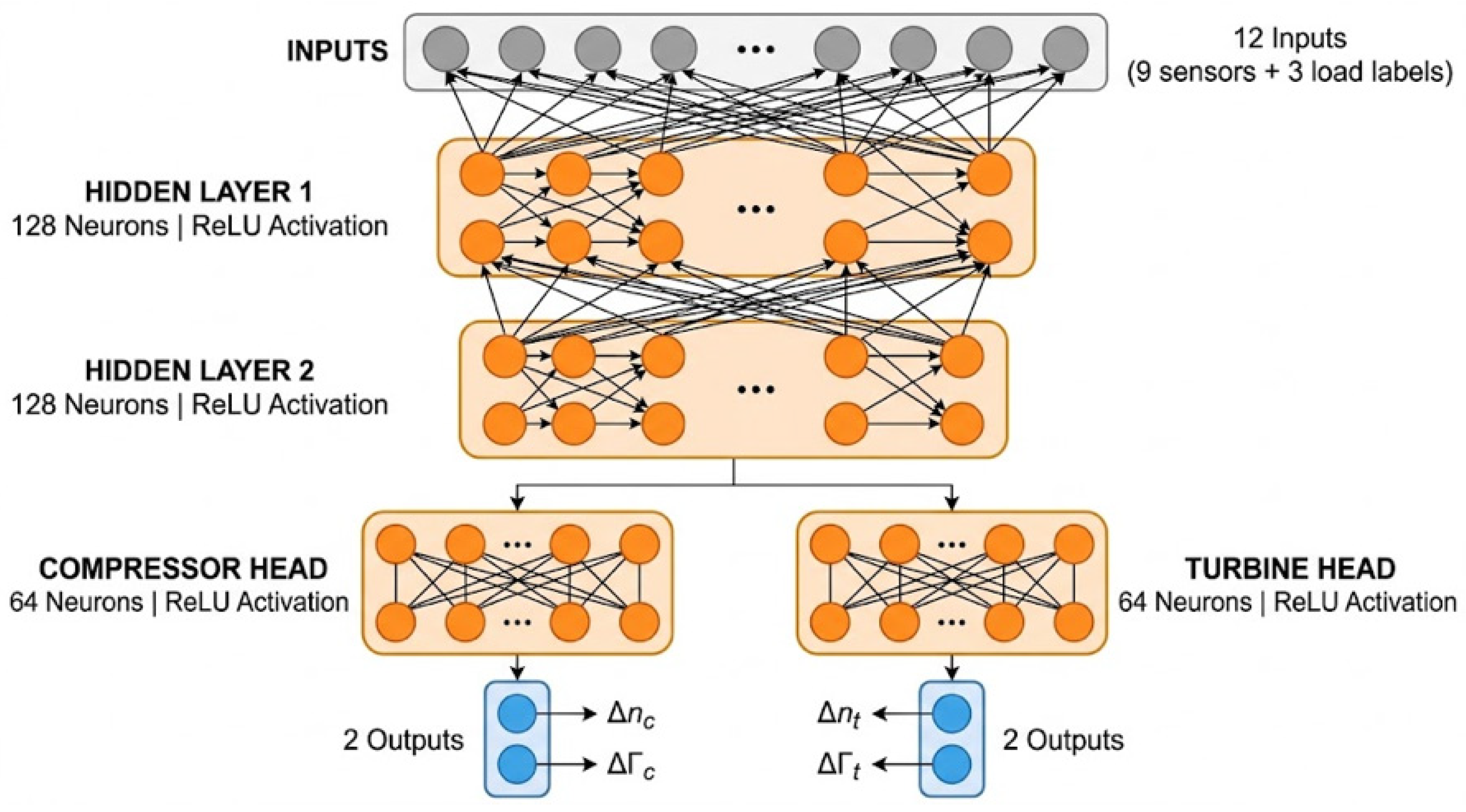
Hyperparameter optimization was performed via randomized search with 5-fold cross-validation, scoring on negative mean absolute error, with each candidate configuration trained for up to 30 epochs under early stopping (patience = 5) to limit search cost (search ranges and selected values in Appendix A, Table A1). The selected configuration was retrained on the full training set for up to 200 epochs using the Adam optimizer with MSE loss, early stopping on validation loss (patience = 15) and best-epoch weight restoration, using a stratified 80/20 validation split of the training data. The final architecture (Figure 11) consists of a shared trunk of two fully connected layers of 128 neurons each, with ReLU activation, Batch Normalization, and Dropout (rate = 0.1) applied after each trunk layer, feeding into two identically structured output heads (Compressor and Turbine), each comprising a single hidden layer of 64 neurons with ReLU activation and Batch Normalization, followed by a linear output layer of 2 neurons.

Figure 11. Final architecture for the MTL-MLP regressor.

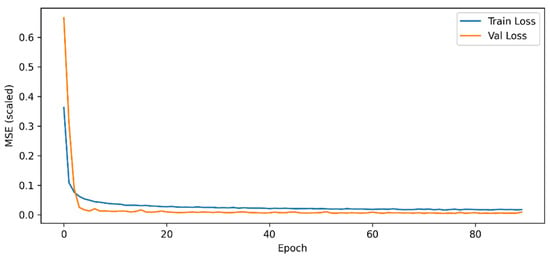
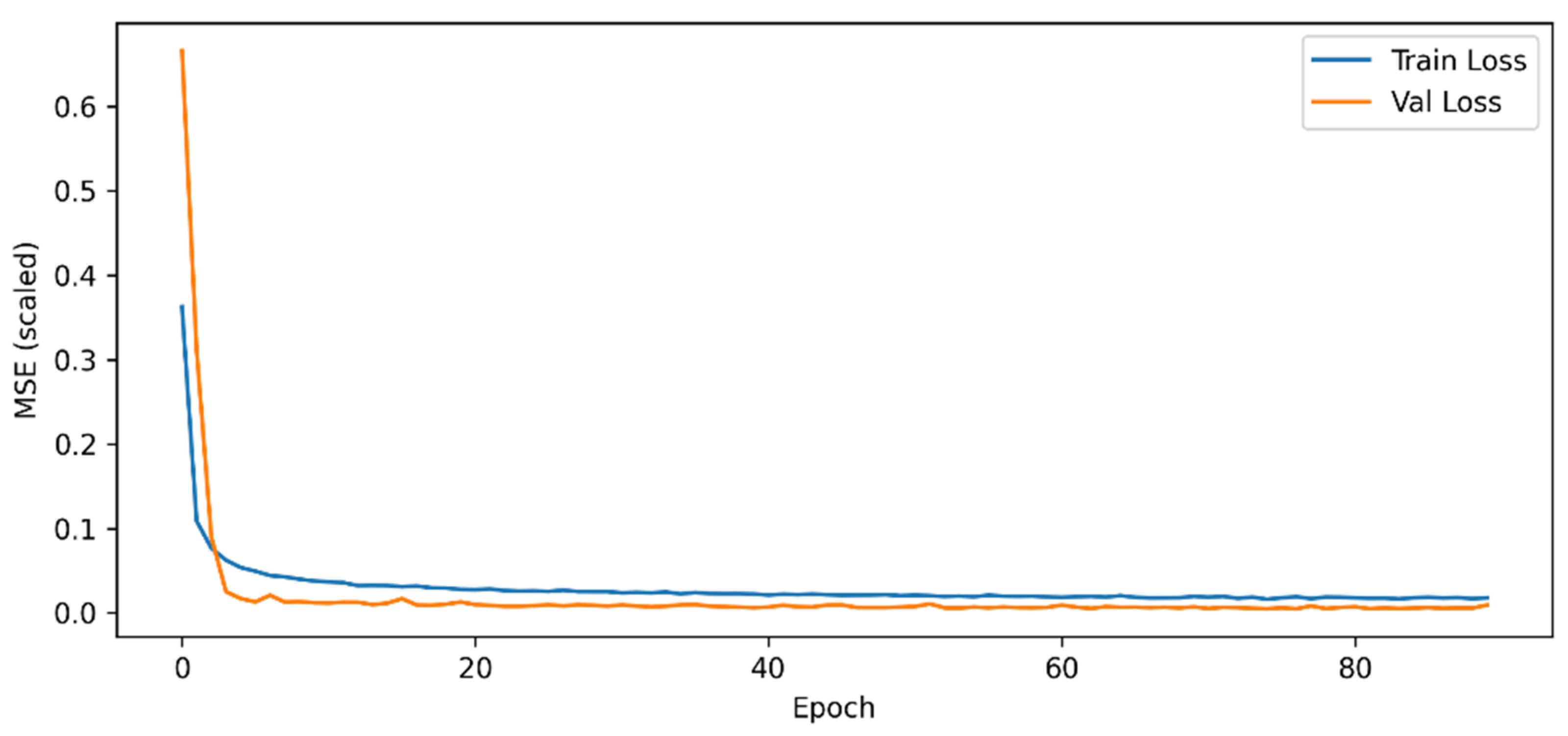
Under this configuration, training and validation performance were in close agreement (Table 6), with training and validation loss curves (Figure 12) declining sharply within the first five epochs and converging to a stable plateau without subsequent divergence—indicating no meaningful overfitting.

Table 6. Overall training and validation metrics of the MTL-MLP regressor.

	R2	RMSE (%)	MAE (%)
Training	0.995	0.102	0.067
Validation	0.995	0.105	0.068

Figure 12. Training and validation loss learning curves for the MTL-MLP regressor.

6. Results

6.1. End-to-End Pipeline Evaluation

The complete diagnostic pipeline was evaluated on the 2880-sample internal test set. Because this dataset also informed algorithm and threshold selection during Stage 1 development (§5.2), the results below should be understood as a confirmatory characterization of pipeline performance rather than a fully independent evaluation; the interpolation and noise-robustness experiments of §6.3, conducted on entirely separate datasets, provide the independent evidence of generalization.

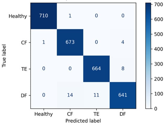
Stage 1—Selective Classification. At the selected threshold θ = 0.85, 2727 samples (94.7%) received a confident prediction, while 153 (5.3%) were routed to Monitoring Mode. On the confident subset, the classifier achieved an overall accuracy of 98.6%. Per-class precision, recall, and F1-score are reported in Table 7, with the corresponding confusion matrix shown in Figure 13.

Table 7. Classification report on confident predictions.

Class	Precision	Recall	F1-Score
Healthy	0.999	0.999	0.999
Compressor Fouling	0.978	0.993	0.985
Turbine Erosion	0.984	0.988	0.986
Double Fault	0.982	0.963	0.972

Figure 13. Confusion matrix of the classification stage.

The Healthy class achieved near-perfect precision, recall, and F1-score, with only two misclassifications among the 711 samples—an operationally important result, since false negatives at the health/fault boundary would suppress a maintenance alert entirely. The Double Fault class showed the lowest recall (96.3%; 25 false negatives among 666 samples), with all errors directed toward the two single-fault classes, consistent with the thermodynamic overlap identified via LDA (Section 4.3). Of the 2727 confidently classified samples, 711 were identified as Healthy and required no further processing, while the remaining 2016 were forwarded to the MTL regressor for severity quantification.

Stage 2—Degradation Quantification. Evaluated per output head, restricted to samples where the corresponding fault is physically active, R² remained above 0.985 and MAE below 0.156 percentage points across all four outputs (Table 8).

Table 8. Regressor performance on the internal test set.

Output	R2	RMSE (%)	MAE (%)
Δnc	0.985	0.171	0.132
ΔΓc	0.986	0.203	0.156
Δnt	0.99	0.070	0.055
ΔΓt	0.99	0.055	0.044

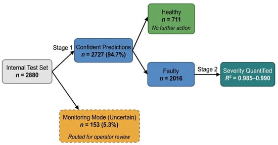
Taken together, of the 2880 internal test samples, 94.7% received a definitive diagnostic outcome—711 correctly identified as Healthy requiring no further action, and 2016 forwarded to the MTL regressor and quantified with R² = 0.985–0.99—while the remaining 5.3% were withheld for operator review, as summarized in Figure 14.

Figure 14. Sample flow through the diagnostic pipeline: routing outcomes and final quantification quality for the internal test set.

Moreover, on a standard laptop without GPU acceleration, the complete pipeline processes a single sample in about 32 ms and the full internal test set in under 0.1 s, so its computational cost poses no practical constraint on real-time condition monitoring.

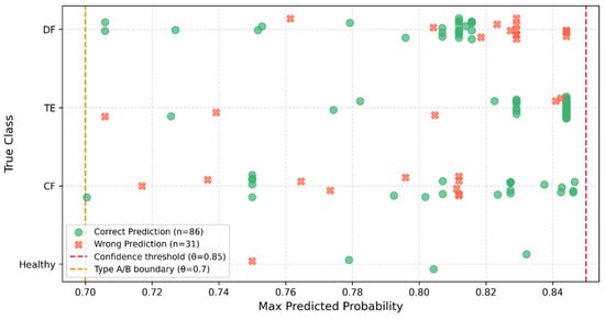
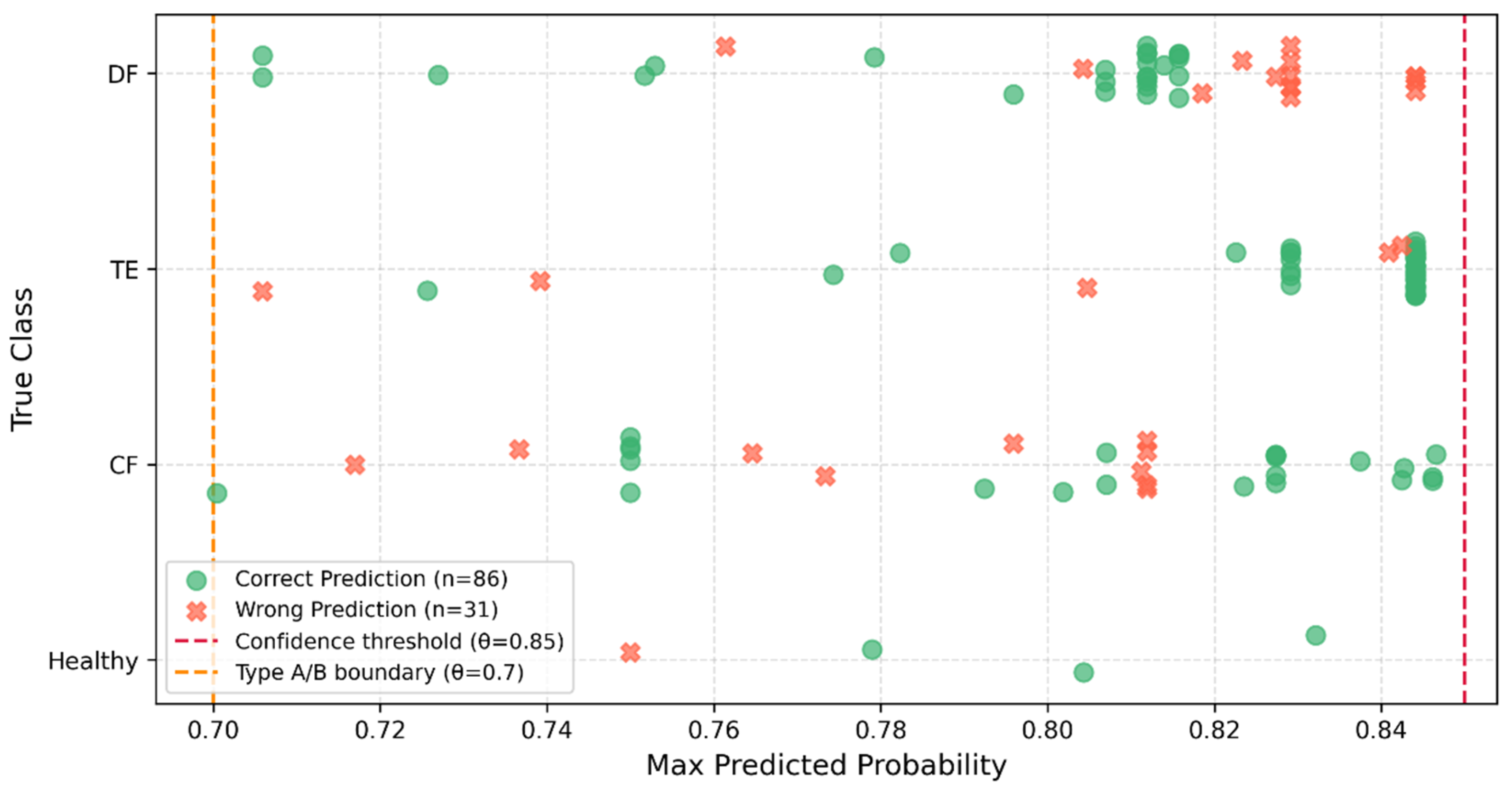
Among the 153 uncertain samples, 117 exhibited a clear leading class despite falling below the confidence threshold—cases where the classifier had a preferred prediction but insufficient confidence to commit (maximum probability in [0.70, 0.85)). Had these samples been assigned to their leading class rather than withheld, only 86 (73.5%) would have received the correct label, meaning roughly one in four would have been misclassified. As shown in Figure 15, these errors are not confined to a particular class or probability sub-range but occur throughout the interval, indicating that the risk of a forced label is distributed across the entire boundary region rather than concentrated near one edge. This result constitutes the clearest evidence for the value of the selective classification mechanism: at precisely the point where the classifier is asked to commit despite marginal confidence, roughly a quarter of forced decisions would be wrong—errors that instead surface as flagged, reviewable cases rather than silent misdiagnoses.

Figure 15. Prediction outcome scatter plot for the boundary uncertain samples.

6.2. Explainability Analysis

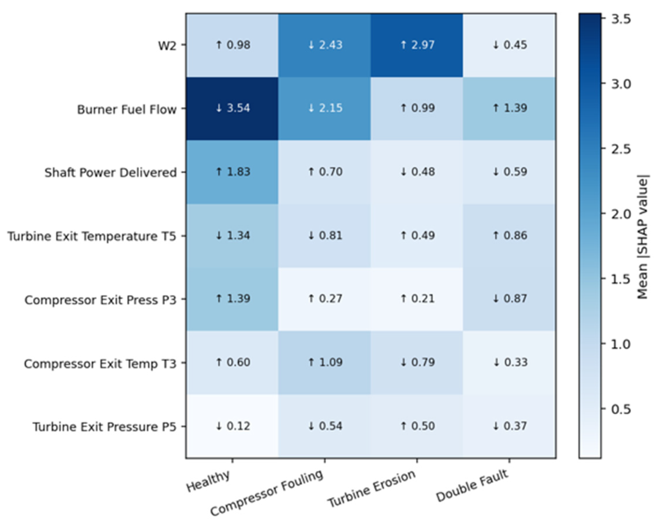
To verify that the diagnostic pipeline’s decisions are grounded in physically consistent reasoning rather than dataset-specific statistical artifacts, SHapley Additive exPlanations (SHAP) were applied to the Stage 1 XGBoost classifier. SHAP values are grounded in cooperative game theory, decomposing each prediction into additive, feature-level contributions that are directly comparable across features and classes [29,30]. The analysis is restricted to the seven gas path sensors; ambient inputs (inlet temperature, relative humidity) are excluded as they encode environmental rather than engine-health information.

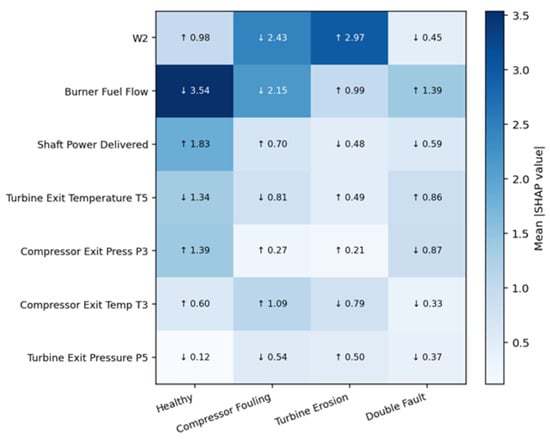
Figure 16 reports the mean absolute SHAP value for each sensor–class pair, annotated with the direction of effect (↑: high sensor values increase the predicted probability of that class; ↓: low values do so). Several patterns align closely with the expected gas-path physics. Compressor Fouling and Turbine Erosion occupy opposite ends of the corrected mass flow (W2) attribution spectrum—low W2 is the dominant driver of Compressor Fouling predictions, consistent with the flow blockage caused by blade-surface deposits, while high W2 dominates Turbine Erosion predictions, consistent with the increased effective flow area of an eroded turbine stage. Burner Fuel Flow is the single strongest attribution in the entire matrix for the Healthy class, with low fuel flow reflecting operation at the nominal design-point fuel schedule; the same sensor drives Turbine Erosion and Double Fault predictions in the opposite direction, consistent with the compensatory fuel increase required to sustain power output as the turbine pressure drop falls. The Double Fault class shows no sensor exceeding a mean |SHAP| of 1.4—substantially below the dominant sensor for each single-fault class (2.43–3.54)—reflecting a diffuse, mixed gas-path signature rather than a single identifiable cause, consistent with the simultaneous presence of both fault mechanisms.

Figure 16. Mean |SHAP value| by sensor and fault class (arrows indicate direction of effect on predicted class probability).

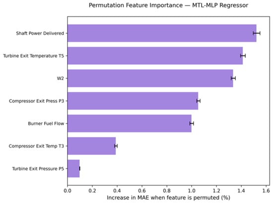
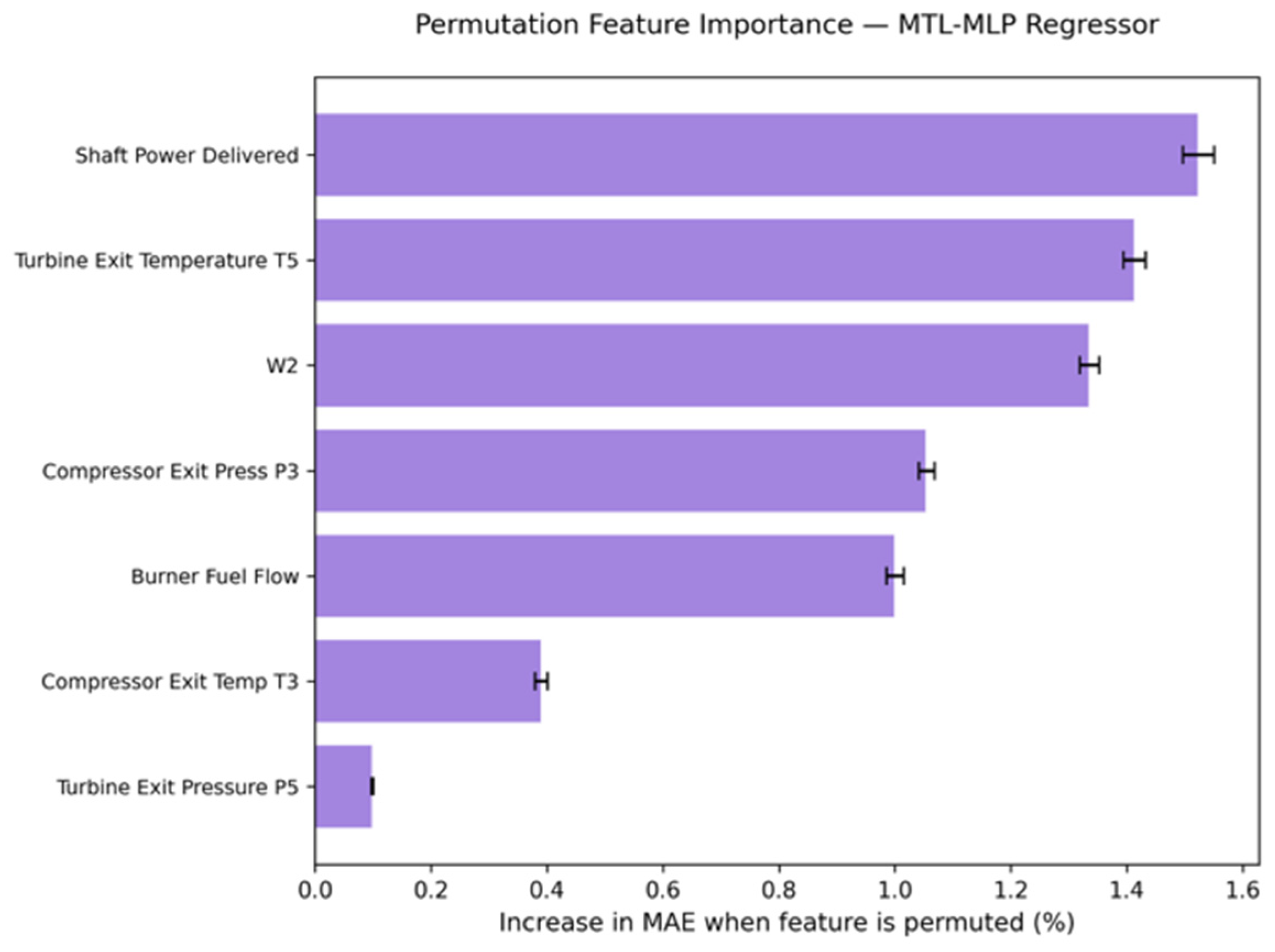
To assess feature dependence in the Stage 2 regressor, permutation importance was additionally computed across all four degradation outputs. Every gas path sensor produced a measurable increase in mean absolute error when permuted, as shown in Figure 17, with no sensor found dispensable—indicating that reliable severity quantification depends on the joint contribution of the full sensor set rather than any single dominant measurement.

Figure 17. Permutation importance for every gas path channel.

The two methods address different questions and are applied to different models, so their sensor rankings are not directly comparable: SHAP provides signed, per-class attributions for the classifier, whereas permutation importance measures the global loss of regression accuracy when a sensor’s information is removed. Their conclusions are nevertheless consistent. In both stages, the models depend on the gas path sensors jointly, and the diffuse SHAP profile of the Double Fault class mirrors the regression finding that no sensor is dispensable: a combined fault is recognized and quantified from the joint pattern of several measurements. Because several sensors are strongly correlated, both methods distribute importance among correlated channels, and rankings are best read at the level of sensor groups rather than individual sensors.

6.3. Robustness Analysis

Three targeted validation experiments assessed the pipeline’s generalization beyond the internal test distribution.

6.3.1. Interpolated Operating Conditions

Three datasets tested generalization to degradation severities unseen during training: intermediate CF/TE levels (3.5, 5.5, 7.5, 9.5) and five unseen DF severity combinations. Stage 1 classification results (Table 9) showed CF and TE coverage (96.9% and 94.2%) consistent with the 94.7% baseline, with accuracy above 99% for both and all errors directed toward DF rather than crossing the Healthy boundary; the DF dataset achieved 100% coverage and 100% accuracy across 450 samples, indicating that the learned DF decision region generalizes to novel severity pairings.

Table 9. Classification stage results on interpolation dataset.

Datasets	Total Samples	Coverage (%)	Uncertain Samples	Classification Accuracy (%)
CF	360	96.9	11	99.7
TE	360	94.2	21	99.1
DF	450	100	0	100

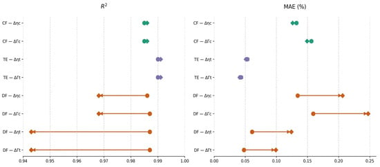
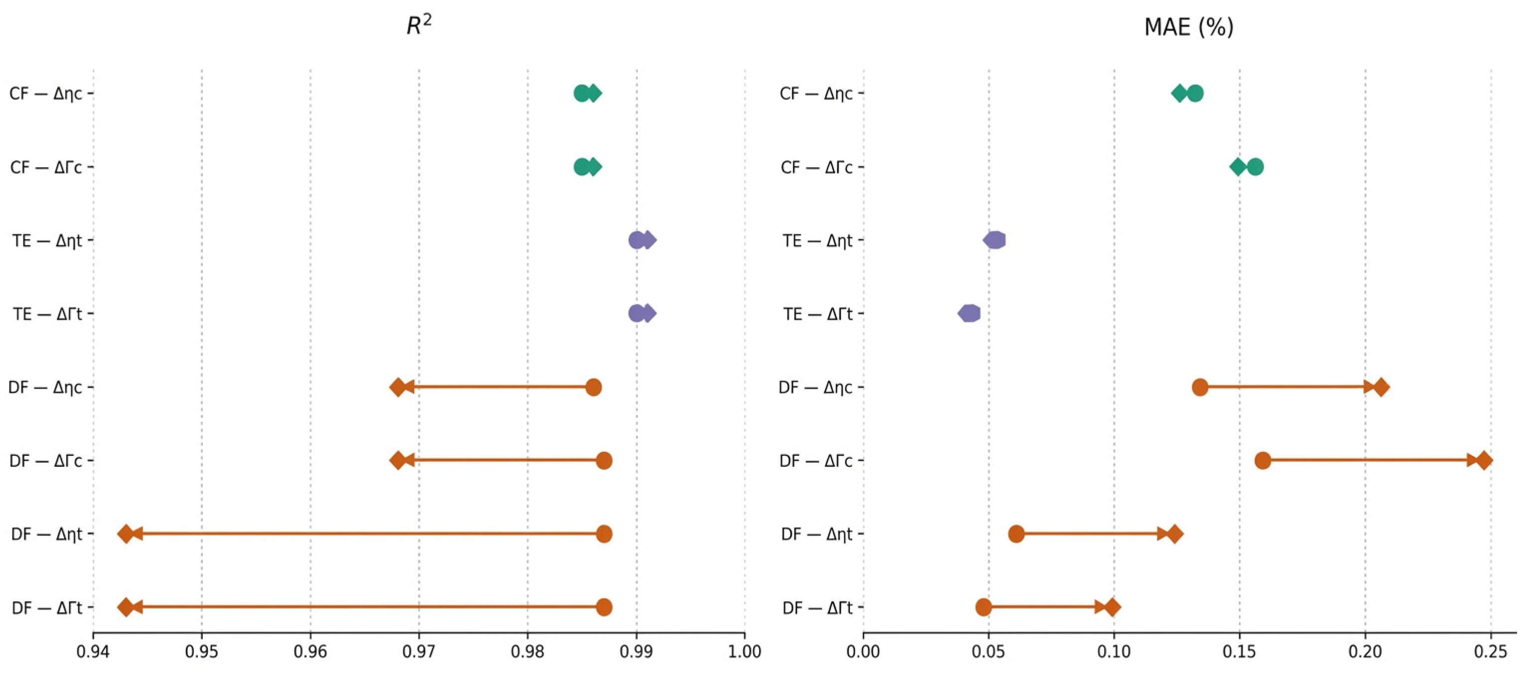
Stage 2 regression performance under interpolated conditions is summarized in Figure 18. For both Compressor Fouling and Turbine Erosion, the internal-test and interpolation markers are essentially coincident: R² remains above 0.98 for all four outputs, and the MAE shift is below 0.002 percentage points, a difference with no practical significance. The Double Fault outputs show a visibly wider gap between the two markers: R² falls to as low as 0.943 for the turbine outputs, and MAE increases by 0.019 to 0.044 percentage points relative to the internal test set, with the turbine outputs showing the larger relative shift in both panels. This is a measurable but operationally bounded reduction in precision, attributable to the incomplete DF severity-combination coverage in the training data noted in Section 3.

Figure 18. Connected dot plot comparing performance metrics between the internal test and interpolation datasets.

6.3.2. Minor Degradation Scenario

Degradation Levels 1–2 (excluded from training) were tested via 360 CF/TE samples. Routing outcomes (Table 10) showed 85.6% of samples routed to either Monitoring Mode (15.3%) or a Healthy classification (70.3%)—both operationally appropriate outcomes at this sub-threshold severity—while 14.4% received a confident but false fault alert. Notably, the 15.3% abstention rate at this scenario, three times the 5.3% baseline rate, suggests Monitoring Mode’s coverage rate could itself serve as a passive statistical indicator of incipient degradation, though this application lies outside the present study’s scope.

Table 10. Routing outcome of the minor degraded samples.

Routing Outcome	Count	Share of Total (%)
Uncertain → Monitoring mode	55	15.3
Confident → Healthy	253	70.3
Confident → Fault alert	52	14.4
Total	360	100

6.3.3. Elevated Noise Conditions

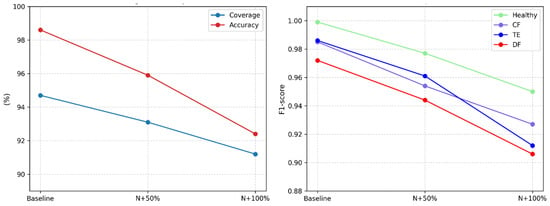
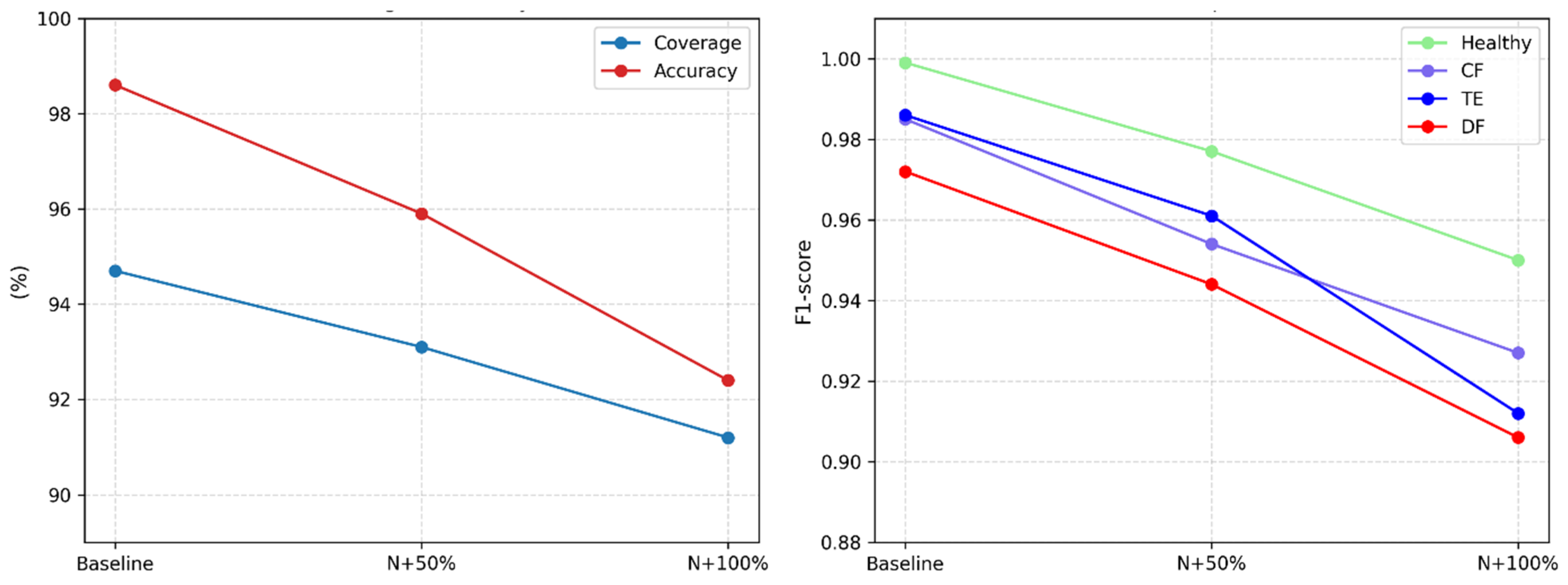
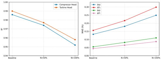
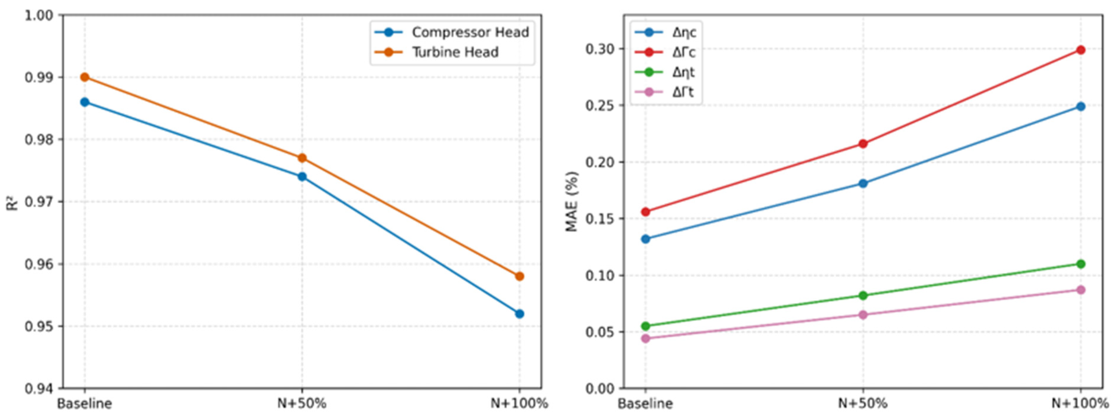
To emulate sensor degradation over time, noise was elevated 50% and 100% above the baseline uncertainty levels used in training, applied to the internal test set. Stage 1 coverage fell from 94.7% (baseline) to 93.1% and 91.2% at +50% and +100%, respectively, while accuracy on confident predictions dropped from 98.6% to 95.9% and 92.4% over the same range; the corresponding per-class F1-score shifts are shown in Figure 19. Stage 2 regression error increased consistently across all four outputs (Figure 20), with turbine outputs showing a larger relative MAE increase (+49% at +50%, +100% at +100%) than compressor outputs (+38%, +91%)—a consequence of their narrower baseline error rather than greater noise sensitivity. Error propagation from Stage 1 misclassifications remained negligible throughout: the largest observed ΔMAE (0.014 percentage points at +100% noise) is an order of magnitude below the noise-induced MAE increase itself.

Figure 19. Classification performance as a function of sensor noise levels. (Left) Overall pipeline coverage and confident-sample accuracy. (Right) Per-class F1 score.

Figure 20. Regression performance as a function of sensor noise levels. (Left) R² for compressor and turbine heads. (Right) MAE (%) for all four outputs.

Taken together, the three robustness experiments define the system’s operating envelope. Within the trained severity range, the pipeline generalizes without meaningful loss, and for unseen Double Fault combinations, quantification precision degrades measurably but remains operationally useful. Sensor noise up to 50% above baseline produces losses that stay practically acceptable; at 100% elevated noise, degradation is more substantial—92.4% accuracy, compressor MAE ≈ 0.3%—though the system remains functional. Degradation below the sensor noise floor (Levels 1–2) is, by design, not reliably detectable: a physical detectability limit rather than a model deficiency, positioning the system as a condition monitor for established faults rather than an early-warning tool for incipient degradation.

7. Discussion

Two gaps in the gas turbine diagnostics literature motivated the two-stage framework developed here—the absence of a calibrated, threshold-based selective classifier with an explicit coverage–accuracy trade-off, and the lack of a multi-task architecture exploiting the physical separation between compressor- and turbine-side degradation for joint parameter quantification—and the results confirm both were addressed. The isotonic-calibrated XGBoost classifier, operated at θ = 0.85, achieved high accuracy on committed predictions while routing ambiguous samples to a dedicated Monitoring Mode rather than forcing an unreliable label. The two-head MTL-MLP regressor produced accurate estimates across all four health parameters, its task-specific heads mirroring the underlying thermodynamic structure and addressing the homogeneous-output limitation of prior fault-quantification approaches. The explainability analysis confirmed that both stages rely on physically meaningful sensor signals, consistent with the fault signatures identified during exploratory analysis.

Taken together, these results show the framework’s core value: replacing periodic manual inspection with a continuous, data-driven layer that quantifies both degradation type and severity from routine gas path measurements. Where traditional condition monitoring relies on time-based schedules and expert judgment, this framework indicates the potential of a continuous, data-driven layer that could complement periodic manual inspection—a step toward shifting gas turbine diagnostics from a reactive to a predictive paradigm.

The robustness evaluation further delineates the system’s practical operating envelope. Within the trained severity range, performance was retained under interpolated degradation levels and previously unseen double-fault combinations, indicating that the learned representations generalize rather than merely memorize training conditions. At incipient degradation levels within the sensor noise floor, the classifier appropriately increased its abstention rate rather than committing to unreliable labels—not a limitation, since normal engine operation already involves comparable baseline wear, so non-detection here reflects a physical detectability boundary rather than a modeling deficiency. Under noise elevated up to 50% above the training distribution, performance losses remained within practically useful bounds; at 100%, degradation was more substantial, particularly for the DF class, and in absolute terms, the compressor-side outputs. Because the threshold acts on calibrated probabilities, its interpretation is independent of operating condition, and under harder conditions, the system responds by lowering coverage rather than by changing its acceptance criterion. The accompanying loss of accuracy on accepted samples at elevated noise indicates, however, that the calibration map fitted at nominal noise becomes optimistic once the noise distribution shifts.

The study is subject to some limitations, leading to further improvements for future research. The dataset was generated entirely through thermodynamic simulation, and no field measurements were used for training or validation, so the reported figures should be read as an upper bound under the present simulation assumptions. Transferring the system to an operating engine would require revalidation against measured data, and since the models include no domain-invariant learning objective, the distribution shift between the simulated and measured data would need to be addressed through domain generalization or adaptation methods [31].

Another point worth noting is that the DF severity space was sampled at 16 out of 64 possible combinations per load, leaving the strongly asymmetric regions of the severity plane uncovered. Two causes contribute to the weaker DF performance. The lower DF recall mainly reflects a physical overlap: when one fault dominates, the combined signature approaches that of a single fault within sensor noise, and all DF misclassifications were indeed assigned to a single-fault class rather than to Healthy. The larger DF interpolation error mainly reflects the sparse coverage, since the same regressor interpolates single-fault severities with no measurable loss. Model capacity is unlikely to be limited, as training and validation performance coincide and all four classifiers showed the same error pattern. Degradation below the sensor noise threshold is, by design, undetectable—positioning the system as a condition monitor for established faults rather than an early-warning tool for incipient degradation.

An additional limitation concerns the balanced class distribution adopted during dataset generation. Although equal representation of the four health states facilitates systematic model development and prevents the underrepresentation of individual fault categories, it does not reflect typical industrial operating conditions, where healthy observations are expected to dominate. Consequently, classification metrics obtained from the balanced test dataset should not be directly extrapolated to operational environments. Future investigations should therefore examine the influence of class imbalance through healthy-state data augmentation, class-weighted or cost-sensitive training, and probability recalibration under representative operational conditions. Performance evaluation should additionally consider prevalence-independent class-conditional discrimination metrics alongside fault-alert precision, false-alarm rates and selective-classification coverage to provide a more representative assessment of the framework’s operational reliability.

Finally, load is represented by three one-hot indicators, so the framework is valid only at 50%, 75%, and 100% of rated power. An operating point between these values has no valid encoding, and the models as trained should not be applied to it; in continuous operation, where load follows grid demand and passes through intermediate values, the present system would therefore cover only part of the operating time. However, overall, the methodology and the results offer a valuable insight into the AI implementation for gas turbine engine diagnostics as guidance for an application to real engine operation.

8. Conclusions

This study developed and evaluated a two-stage machine learning diagnostic framework for fault detection and severity estimation in industrial gas turbines, targeting a single-shaft, GE 7HA.03-inspired heavy-duty gas turbine model. Starting from a thermodynamically validated cycle simulation and a NASA-adapted damage propagation model, a synthetic dataset spanning four health states, eight degradation severity levels, and three load conditions were generated to train and evaluate the proposed pipeline.

The Stage 1 selective classifier, built on a calibrated XGBoost model, achieved 98.6% classification accuracy on committed predictions at a confidence threshold of θ = 0.85, with 94.7% of test samples receiving a definitive diagnostic outcome and the remaining 5.3% correctly routed to Monitoring Mode for human review. The Stage 2 regressor quantified compressor and turbine health parameters through dedicated output heads, achieving an R² above 0.985 and MAE below 0.156 percentage points across all four degradation parameters. These results confirm that the two-stage framework meets its diagnostic objectives: reliable fault identification under realistic sensor noise, a controlled and principled abstention mechanism, and accurate severity estimation across all three fault classes and eight degradation levels. The robustness evaluation further confirmed that this performance generalizes within the trained fault space and degrades predictably, rather than catastrophically, under elevated sensor noise.

The principal contribution of this work is methodological. It demonstrates that a formally calibrated selective classifier with an explicit coverage–accuracy operating point, combined with a physically structured MTL regression architecture, can be integrated into a single diagnostic pipeline for industrial gas turbines—addressing two specific gaps in the existing literature. When a diagnostic system withholds judgment on ambiguous cases rather than forcing a label, the abstention itself carries diagnostic information, marking the boundary of what the model can resolve with confidence.

While these results are grounded in simulation, and field deployment will require further validation against measured operational data, this work establishes that selective classification combined with multi-task regression is a viable and interpretable framework for gas turbine condition monitoring. Future work should prioritize four directions. Replacing the three one-hot load indicators with a continuous load input would remove the restriction to discrete operating points. Shaft power is already among the measured inputs, and normalized by rated power, can serve this purpose directly, provided that the training data are regenerated over a continuous 50–100% load range; neither the tree-ensemble classifier nor the MTL regressor requires architectural changes. Secondly, extending the DF training campaign to cover the asymmetric regions of the severity plane would directly address the largest remaining source of quantification error. Thirdly, because the calibration map fitted at nominal noise becomes optimistic once sensor characteristics drift, the fixed operating point could be replaced by an adaptive scheme in which the probability map is periodically recalibrated on recent data and θ is re-derived to maintain a target error rate on accepted predictions. Finally, relaxing the uniform noise-amplification assumption in favor of heterogeneous, time-varying sensor degradation models—potentially via an upstream denoising or sensor-health-monitoring stage—would close the remaining gap between the simulation environment and field conditions, the step that ultimately determines this framework’s practical value.

References

- Kurz, R.; Brun, K.; Wollie, M. Degradation Effects on Industrial Gas Turbines. J. Eng. Gas. Turbines Power 2009, 131, 062401. [Google Scholar] [CrossRef] [Scilit]
- Kurz, R.; Brun, K. Degradation in Gas Turbine Systems. J. Eng. Gas. Turbines Power 2001, 123, 70–77. [Google Scholar] [CrossRef] [Scilit]
- Burnes, D.; Kurz, R. Performance Degradation Effects in Modern Industrial Gas Turbines. In Proceedings of the Zurich Global Power and Propulsion Forum, Zurich, Switzerland, 10–12 January 2018; Volume 124. [Google Scholar]
- Fentaye, A.D.; Ul-Haq Gilani, S.I.; Baheta, A.T.; Li, Y.-G. Performance-Based Fault Diagnosis of a Gas Turbine Engine Using an Integrated Support Vector Machine and Artificial Neural Network Method. Proc. Inst. Mech. Eng. Part A J. Power Energy 2019, 233, 786–802. [Google Scholar] [CrossRef] [Scilit]
- Fentaye, A.D.; Baheta, A.T.; Gilani, S.I.; Kyprianidis, K.G. A Review on Gas Turbine Gas-Path Diagnostics: State-of-the-Art Methods, Challenges and Opportunities. Aerospace 2019, 6, 83. [Google Scholar] [CrossRef] [Scilit]
- De Castro-Cros, M.; Velasco, M.; Angulo, C. Machine-Learning-Based Condition Assessment of Gas Turbines—A Review. Energies 2021, 14, 8468. [Google Scholar] [CrossRef] [Scilit]
- Molla Salilew, W.; Ambri Abdul Karim, Z.; Alemu Lemma, T. Investigation of Fault Detection and Isolation Accuracy of Different Machine Learning Techniques with Different Data Processing Methods for Gas Turbine. Alex. Eng. J. 2022, 61, 12635–12651. [Google Scholar] [CrossRef] [Scilit]
- Hashmi, M.B.; Mansouri, M.; Fentaye, A.D.; Ahsan, S.; Kyprianidis, K. An Artificial Neural Network-Based Fault Diagnostics Approach for Hydrogen-Fueled Micro Gas Turbines. Energies 2024, 17, 719. [Google Scholar] [CrossRef] [Scilit]
- Togni, S.; Nikolaidis, T.; Sampath, S. A Combined Technique of Kalman Filter, Artificial Neural Network and Fuzzy Logic for Gas Turbines and Signal Fault Isolation. Chin. J. Aeronaut. 2021, 34, 124–135. [Google Scholar] [CrossRef] [Scilit]
- Geifman, Y.; El-Yaniv, R. SelectiveNet: A Deep Neural Network with an Integrated Reject Option. arXiv 2019, arXiv:1901.09192. [Google Scholar] [CrossRef] [Scilit]
- Montazeri-Gh, M.; Nekoonam, A. Gas Path Component Fault Diagnosis of an Industrial Gas Turbine under Different Load Condition Using Online Sequential Extreme Learning Machine. Eng. Fail. Anal. 2022, 135, 106115. [Google Scholar] [CrossRef] [Scilit]
- Romesis, C.; Aretakis, N.; Mathioudakis, K. Model-Assisted Probabilistic Neural Networks for Effective Turbofan Fault Diagnosis. Aerospace 2024, 11, 913. [Google Scholar] [CrossRef] [Scilit]
- Castillo, I.G.; Loboda, I.; Pérez Ruiz, J.L. Data-Driven Models for Gas Turbine Online Diagnosis. Machines 2021, 9, 372. [Google Scholar] [CrossRef] [Scilit]
- Ruder, S. An Overview of Multi-Task Learning in Deep Neural Networks. arXiv 2017, arXiv:1706.05098. [Google Scholar] [CrossRef] [Scilit]
- Zhang, Y.; Yang, Q. A Survey on Multi-Task Learning. IEEE Trans. Knowl. Data Eng. 2022, 34, 5586–5609. [Google Scholar] [CrossRef] [Scilit]
- HA Gas Turbine. Available online: https://www.gevernova.com/gas-power/products/gas-turbines/7ha (accessed on 23 August 2026).
- Li, Y.G.; Pilidis, P.; Newby, M.A. An Adaptation Approach for Gas Turbine Design-Point Performance Simulation. J. Eng. Gas. Turbines Power 2006, 128, 789–795. [Google Scholar] [CrossRef] [Scilit]
- Chapman, J.W.; Lavelle, T.M.; Litt, J.S. Practical Techniques for Modeling Gas Turbine Engine Performance. In Proceedings of the 52nd AIAA/SAE/ASEE Joint Propulsion Conference, Salt Lake City, UT, USA, 25–27 July 2016. [Google Scholar]
- Saxena, A.; Goebel, K.; Simon, D.; Eklund, N. Damage Propagation Modeling for Aircraft Engine Prognostics. In Proceedings of the 2008 International Conference on Prognostics and Health Management (PHM 2008), Washington, DC, USA, 6–9 October 2008. [Google Scholar]
- GE Vernova Heavy-Duty Gas Turbine Operating and Maintenance Considerations-GER-3620P. Available online: https://www.gevernova.com/gas-power/resources/technical-downloads/ger-3620p-operation-maintenance-considerations (accessed on 23 August 2026).
- Meher-Homji, C.B.; Chaker, M.A.; Motiwala, H.M. Gas Turbine Performance Deterioration. In Proceedings of the 30th Turbomachinery Symposium, Houston, TX, USA, 17–20 September 2001. [Google Scholar]
- Diakunchak, I.S. Performance Deterioration in Industrial Gas Turbines. J. Eng. Gas. Turbines Power 1992, 114, 161–168. [Google Scholar] [CrossRef] [Scilit]
- ISO/IEC Guide 98-3:2008; Uncertainty of Measurement: Part 3: Guide to the Expression of Uncertainty in Measurement (GUM:1995). ISO: Geneva, Switzerland, 2008. Available online: https://www.iso.org/standard/50461.html (accessed on 23 August 2026).
- High Accuracy Temperature Sensors|AMETEK Aerospace & Defense. Available online: https://www.ameteksfms.com/products/temperature-sensors (accessed on 23 August 2026).
- Pressure Transducer Specs. Available online: https://www.dwyeromega.com/en-us/resources/pressure-transducer-specs (accessed on 23 August 2026).
- ASME PTC 22-2005; Performance Test Code on Gas Turbines. American Society of Mechanical Engineers: New York, NY, USA, 2005.
- Van Millingen, R.D.; Van Millingen, J.D. Phase Shift Torquemeters for Gas Turbine Development and Monitoring. In Proceedings of the ASME 1991 International Gas Turbine and Aeroengine Congress and Exposition, Orlando, FL, USA, 3–6 June 1991; Volume 5, p. V005T15A003. [Google Scholar]
- Burdett, D.; Hambidge, C.; Povey, T. Analysis of Ultra-Low Uncertainty Gas Turbine Flow Capacity Measurement Techniques. Proc. Inst. Mech. Eng. Part A J. Power Energy 2021, 235, 1053–1079. [Google Scholar] [CrossRef] [Scilit]
- Sun, X.; Yao, Y.; Wang, X.; Li, P.; Li, X. AI-Driven Health Monitoring of Distributed Computing Architecture: Insights from XGBoost and SHAP. In Proceedings of the 2024 4th International Conference on Communication Technology and Information Technology (ICCTIT), Guangzhou, China, 27–29 December 2024; IEEE: Guangzhou, China, 2024; pp. 480–484. [Google Scholar]
- Nor, A.K.M.; Pedapati, S.R.; Muhammad, M. Application of Explainable AI (Xai) For Anomaly Detection and Prognostic of Gas Turbines with Uncertainty Quantification. Preprints 2021, 2021090034. [Google Scholar] [CrossRef]
- Chen, Z.; Lin, H.; Gao, Y.; He, J.; Li, Z.; Li, W.; Liu, Q. Multiscale Scattering Forests: A Domain-Generalizing Approach for Fault Diagnosis under Data Constraints. Knowl.-Based Syst. 2026, 337, 115389. [Google Scholar] [CrossRef] [Scilit]
Disclaimer/Publisher’s Note: The statements, opinions and data contained in all publications are solely those of the individual author(s) and contributor(s) and not of MDPI and/or the editor(s). MDPI and/or the editor(s) disclaim responsibility for any injury to people or property resulting from any ideas, methods, instructions or products referred to in the content. |
© 2026 by the authors. Licensee MDPI, Basel, Switzerland. This article is an open access article distributed under the terms and conditions of the Creative Commons Attribution (CC BY) license.