


Abstract
Efficient path planning for dual crane cooperative systems is a complex challenge due to high-dimensional configuration spaces and the volatile nature of dynamic construction environments. Conventional sampling-based algorithms often suffer from computational delays and lack the ability to adapt to environmental changes without restarting the search process from scratch. This paper proposes a fast path planning and re-planning framework that integrates a 4-DOF reduced-space sampling strategy with a tree-reuse multiple-RRT mechanism. By constraining the sampling space to critical kinematic degrees of freedom and maintaining pre-explored valid nodes as a persistent knowledge base, the framework enables rapid initial planning and near-real-time response to unperceived obstacles. Experimental results demonstrate that the 4-DOF sampling significantly reduces total planning time compared to conventional 6-DOF methods, with superior performance particularly in restricted narrow-path scenarios. Furthermore, the tree-reuse strategy facilitates efficient path re-initialization, substantially reducing re-planning time and exhibiting a notable learning effect in sequential transport tasks through accelerated convergence. These findings demonstrate that the proposed framework effectively mitigates the “new node exploration” bottleneck, offering a robust and practical solution for autonomous dual crane coordination in complex construction sites.
1. Introduction
As construction and civil engineering projects become increasingly large-scale, the role of mobile cranes in precisely transporting heavy loads has become more critical than ever. In particular, at sites where the operation of ultra-large cranes is restricted due to economic costs, soil bearing capacity limits, or narrow workspaces, the dual crane cooperative lifting method—operating two cranes in parallel—is gaining significant attention as a practical alternative [1,2,3,4,5]. Beyond simply overcoming physical load limits, this method provides the advantage of kinematically suppressing the yaw swing phenomenon, which is a chronic issue in single-crane lifting, by supporting the workpiece at two points, thereby dramatically improving overall system stability [6].
Despite these advantages, cooperative lifting systems pose significant control challenges due to increased degrees of freedom (DOF) and complex kinematic characteristics [7]. Due to the nature of closed-loop kinematics involved in transporting a shared load, precise synchronization between operators is essential. Organic coordination between the two machines is required to prevent system rollover and collisions with the workpiece or surrounding obstacles. Generally, since the visual information available inside the cockpit is very limited, close collaborative work involving multiple personnel, including external spotters, is necessary. This reliance on human coordination often leads to a high degree of variability in safety and efficiency, as the performance is heavily dictated by the skill levels and collaborative experience of the individual operators [8].
In such highly complex lifting scenarios, traditional manual planning methods have limitations in fully guaranteeing operational precision and safety. Consequently, the introduction of reliable automated path planning technology has emerged as an essential requirement. Automation plays a key role in proactively preventing human errors that can lead to accidents and lowering potential risks on-site by pre-validating the feasibility of planned paths through simulation. Furthermore, by providing intuitive motion guidance through digital interfaces, these technologies enable even less experienced operators to safely complete high-difficulty tasks, which is considered a fundamental capability that must be secured at the forefront of smart construction automation.
Previous studies on automated path planning have proposed various methodologies such as Genetic Algorithms (GA), A* algorithms, and Probabilistic Roadmaps (PRM) [9], but most have been limited to single crane applications [3,8,10,11,12,13]. Extending these to dual-crane cooperative systems presents technical hurdles where the C-space expands rapidly and the computational load increases exponentially as the system’s DOF doubles [7,14]. Additionally, the considerations for kinematic stability constraints to prevent interference and rollover increase significantly [6]. To address these issues, early studies proposed Hill-climbing and A* algorithms [15], but the Hill-climbing method was prone to falling into local minima, and the computation time increased sharply with environment complexity. Subsequent attempts used Genetic Algorithms [4] for path search and optimization, but these consumed a substantial amount of computational resources. Studies based on PRM [3] reduced the computational load by introducing excessive kinematic constraints, yet this often deviated from realistic dual crane operating environments. While Parallel Genetic Algorithms [5] meticulously considered kinematic chains, they were either dependent on high-performance computing resources or limited to relatively simple scenarios. To reliably generate paths in high-dimensional C-space, recent research introduced a Multiple RRT strategy [6,16,17,18], effectively solving the challenging ‘narrow path finding’ scenario where the system must pass through tight spaces under complex kinematic constraints [6]. That study efficiently explored high-dimensional C-space by generating and growing new trees whenever a node could not be connected to existing trees, successfully deriving solutions for high-difficulty scenarios. However, that search was carried out over the full six-dimensional C-space against an obstacle set taken as fixed, and the trees were not retained once a path had been found, so neither the cost of sampling the full space nor the response to a change in the environment was addressed. A separate line of work addresses the sampling problem itself, for systems in which kinematic constraints restrict the admissible configurations to a lower-dimensional subset. Projection-based planners draw a sample in the full space and move it onto the constraint manifold by iterated gradient descent [19]; atlas-based planners instead cover the manifold with local charts built from tangent spaces and sample within them [20]; and a survey of these families, including the case in which a system admits a re-parameterization that yields admissible configurations directly, is given in [21]. The dual crane falls into that last case: its closed-chain condition can be solved in closed form, so that the variables which are not sampled are obtained algebraically rather than by projecting a sample onto the manifold or by maintaining a chart that approximates it. The sampler proposed in this paper exploits that property, and the reduction in the sampling space from six dimensions to four follows from it.
A separate line of recent work replaces part of the planning computation with a learned model. Reinforcement learning has been combined with imitation learning from operator demonstrations to produce tower crane lift paths [22], deep reinforcement learning has been applied to online lifting in environments that are not known in advance [23], and the same pattern of a policy trained offline and queried online is reported across navigation and motion planning more generally [24]; learning has also been introduced inside sampling-based planners, by training the distribution from which samples are drawn so that the search concentrates on regions likely to contain a solution [25]. These methods require a training stage and a set of environments to train on, and the resulting policy is tied to the crane and the site it was trained for, which limits their use where a lift is planned once against the geometry of a single BIM model. Stability can also be pursued at the execution layer rather than at the planning layer, as in the phase-plane intervention criterion that decides when active front steering should assist the driver of an emergency rescue vehicle [26], although such methods act on a motion whose geometry has already been fixed.
Nevertheless, a common challenge faced by these previous studies is the immense computational time and high processing power required for path generation. Although the Multiple RRT strategy significantly improved the computational load [6], limitations remain as scenarios with high kinematic difficulty still require considerable time to find a valid solution. This problem becomes even more pronounced when combined with the variable nature of actual construction sites. Paths are generally generated based on Building Information Modeling (BIM) data; however, BIM models may not perfectly reflect all temporary facilities (scaffolding, supports, etc.) or there may be discrepancies between actual structure positions and digital data. Such ‘temporal obstacles’ that are not accounted for in the planning stage undermine the reliability of conventional methods that rely solely on static data, potentially leading to unforeseen collisions during transport [27]. While modern systems utilize LiDAR or camera-based monitoring to detect obstacles in real time [28,29,30], the approach of re-generating the entire path from scratch every time a new obstacle is discovered degrades overall construction efficiency and reduces real-time responsiveness. Outside the crane literature, several sampling-based planners address this by retaining part of the previous computation instead of discarding it. RT-RRT* keeps a single tree and moves its root as the agent advances, rewiring the branches that the change invalidates [31]; a planner for real-time navigation carries a cache of waypoints from the previous solution into the next query [32]; RRT*-FN bounds the number of stored nodes and removes the least useful of them as new ones are added [33,34]; and BIT* reuses the information gathered in earlier batches of samples as the graph is densified within a single query [35]. These mechanisms differ in what they preserve and in how a portion of the structure that becomes disconnected is treated, and the distinction from the method proposed here is set out in Section 3.2.
To overcome these limitations, this study proposes an Experience-Based Planning framework that leverages previously explored search data. The necessity for real-time path re-planning and tree information reuse is not only confined to sudden obstacle avoidance. In actual construction sites, repetitive lifting operations—where a dual crane system at a fixed position must continuously lift multiple girders or large steel members to various adjacent target locations—occur frequently. In such scenarios, researching the entire C-space for every single task is an extreme waste of computational resources. In contrast, the Experience-Based Planning approach treats the vast search trees constructed during the initial path generation as a persistent knowledge base rather than discarding them. This allows for the immediate derivation of paths based on previously explored feasible space information during consecutive subsequent lifting tasks, drastically reducing the time required for each re-planning instance. Furthermore, since optimization is performed based on broadly validated spatial topology, it offers the decisive advantage of simultaneously enhancing both the path quality and the consistency of the operation. Appendix A sets out, for the studies discussed above, the target system, the planning approach, the response to a change in the environment and the extent to which previous computation is reused. The crane studies that respond to a change in the environment do so for a single crane, or for cranes that carry separate loads rather than a shared one, and the planners that retain part of a previous computation were developed for a single agent moving freely. The combination addressed here, a closed-chain dual crane re-planned from retained and individually validated search data, does not appear among them.
Consequently, this study proposes a fast path planning and re-planning framework that integrates experience-based planning principles to respond effectively to both temporal obstacles and repetitive operations. By synergistically combining a reduced-space sampling strategy to accelerate search efficiency with a tree-reuse mechanism for rapid path updates, the proposed algorithm significantly overcomes the computational bottlenecks of traditional dual crane coordination. The primary contributions of this research are as follows:
First, the search space was reduced from the conventional 6-DOF to 4-DOF by imposing constraints that fix the girder and cable angles to zero during exploration. Furthermore, by defining the swing angle in polar coordinates and efficiently limiting the search space through pre-calculated exclusion zones, the time required for tree expansion was drastically shortened [36,37].
Second, to enable rapid response to newly detected obstacles or repetitive lifting tasks, the tree information constructed during initial path generation is transformed into a persistent database for maximum reuse rather than being discarded [31,32,33]. By removing only the nodes overlapping with the obstacle and rapidly reconnecting the remaining subtrees through tree reuse, the re-planning speed has been significantly improved.
The remainder of this paper is organized as follows. Section 2 presents the kinematic modeling of the dual crane system and defines the fundamental constraints for cooperative lifting. Section 3 details the proposed experience-based planning framework, including the 4-DOF reduced-space sampling and the tree reuse for rapid re-planning. Section 4 validates the performance of the proposed algorithm through various simulation scenarios, comparing it with conventional methods. Finally, Section 5 concludes the paper with a summary of findings and suggestions for future research.
2. Kinematic Modeling and System Constraints
2.1. System Modeling of the Dual Crane System
The dual crane cooperative system investigated in this study consists of two mobile cranes, designated as Crane1 and Crane2, which jointly manipulate a single shared payload (P). This configuration inherently forms a closed-loop kinematic chain during the lifting and transport process. Under normal operating conditions, the motion of a single mobile crane with a fixed base is generally defined by four degrees of freedom (DOFs): the swing angle (θi), the boom luffing angle (φi), the boom length (lb,i), and the hoist rope length (lh,i) where i = 1,2 represents each crane, as illustrated in Figure 1.
Figure 1.
Coordinates of dual crane system.
However, in practical lifting scenarios, the boom length is strictly maintained at a constant value to ensure structural integrity and load-bearing stability. Consequently, each individual crane is effectively treated as a 3-DOF system. By coupling two such cranes, the dual crane cooperative system operates within a 6-dimensional configuration space (C-space) [6,38].
A specific state of the dual crane system is represented by the configuration vector C, defined as follows:
C = (θ1,φ1,lh,1,θ2,φ2,lh,2)
Within this C-space, a trajectory for the dual crane system, denoted as Pathdual, is defined as an ordered sequence of discrete configurations:
Pathdual = {C1,C2,C3…,Cn}
This ordered sequence of configurations defines the system’s trajectory from an initial state to a target state.
2.2. Suspension Subsystem Modeling and Equilibrium Analysis
The payload system suspended by two cranes can be kinematically modeled as a four-bar linkage structure. The boom tips of each crane (A1,A2) and the anchor points of the payload (B1,B2) form the vertices of this structure, which are connected by hoisting cables (lh,1,lh,2) and the fixed length of the payload (lload), thereby establishing a physical closed loop.
In an equilibrium state, the two boom tips, the two anchor points, and the center of gravity (CG) of the payload are aligned within the same vertical plane. This characteristic allows for a geometric analysis of the system in a two-dimensional plane, as illustrated in Figure 2. This kinematic chain must satisfy the following closed-loop equality constraints:
Horizontal Constraint: x1 + lh,1sin(ϕh,1) + lloadcos(ϕload) + lh,2sin(ϕh,2) = x2
Vertical Constraint: z1 − lh,1cos(ϕh,1) + lloadsin(ϕload) + lh,2cos(ϕh,2) = z2
Figure 2.
Suspension subsystem in dual crane system.
Furthermore, for such a closed-loop system to be physically valid, it must maintain a state of gravitational equilibrium, which is defined by the following force and moment balance conditions:
To solve this highly nonlinear equilibrium problem, this study adopts the numerical methodology from previous research [6]. A suspension system within a gravitational field tends to converge to a state where potential energy is minimized, provided no external energy is applied. Therefore, the numerical solution is derived by leveraging the physical property that the system achieves static equilibrium when the center of gravity (CG) of the payload is positioned at the lowest reachable point within the kinematic constraints. This approach allows the equilibrium payload attitude (ϕload) and cable angles (ϕh,i) to be determined efficiently at each sampling node without the need to solve complex simultaneous equations directly, thereby maximizing computational efficiency.
2.3. Feasibility Check for Path Generation
To ensure the reliability of automated path planning, every generated configuration C must be verified against a set of predefined constraints. This verification process is referred to as the “feasibility check” for configuration C, ensuring that the planned path is practically executable and safe within the given environment.
2.3.1. Slope and Operational Constraints
To maintain stability during transport, the system must adhere to the following two angular constraints.
- Hoist Cable Slope (ϕh,i): The angle between the hoist cable and the vertical line must be maintained within a specific threshold (ϕh,max). Exceeding this limit can result in excessive horizontal force components, which may induce payload sway or apply critical side loads to the crane boom, potentially compromising the structural integrity of the equipment.
- Payload Slope (ϕload):The inclination of the payload is also restricted within a maximum allowable angle (ϕload,max) to prevent sudden load shifting and ensure stability during the lifting process.
2.3.2. Collision Avoidance and Detection
All components of the dual crane system must avoid physical contact or interference with the following entities.
- Self and Crane-to-Crane Collision: This involves preventing interference between the internal components of an individual crane, as well as physical collisions between the two cranes operating within the shared workspace.
- Obstacle and Ground Collision: This ensures the avoidance of interference between the payload and surrounding structures, including constraints to prevent unintended contact between the payload and the ground during transport.
For computational efficiency in collision checking, obstacles at the construction site are defined as rectangular box models. These geometric regions are specified using the 3D coordinates of two diagonally opposite vertices, where the subscript i identifies each obstacle in the set:
All system components are modeled using bounding boxes or bounding cylinders. In this study, the GJK (Gilbert-Johnson-Keerthi) algorithm, integrated into the MATLAB 2024b Robotics System Toolbox, was employed to rigorously verify geometric interference, ensuring both the accuracy and computational speed of the collision detection process.
The proposed framework rests on the following assumptions, which define its scope and limitations.
- Fixed boom length: the boom length of each crane is kept constant during transport, so that each crane is treated as a 3-DOF system and the dual crane system operates in a 6-dimensional C-space.
- Quasi-static equilibrium: at every planned configuration the payload–cable subsystem is assumed to be in static equilibrium (Section 2.2); transient cable and payload sway are not modeled.
- Geometric environment model: obstacles are represented by axis-aligned bounding boxes, and all crane components and the payload by bounding boxes or cylinders; an obstacle is treated as stationary once it has been detected.
- Ideal obstacle detection: newly appearing obstacles are assumed to be detected without latency or false positives, and the system is assumed to come to rest in a statically balanced configuration before re-planning starts (Section 3.2).
- Geometric path output: the planner produces a collision-free geometric path in the C-space; velocity and acceleration limits of the cranes are to be handled by a subsequent trajectory-generation stage, which is outside the scope of this paper.
3. Proposed Method
The planning problem addressed in this paper is stated as follows. Given the base positions and boom lengths of the two cranes, the payload dimensions, the obstacle set of Equation (7) obtained from the BIM model, the allowable thresholds on the cable and payload slopes, and the pick and place configurations, find an ordered sequence of configurations of the form of Equation (2), in the six-dimensional C-space of Equation (1), that begins at the pick configuration and ends at the place configuration, subject to the feasibility check of Section 2.3 holding at every configuration of the sequence and at every intermediate configuration obtained by interpolating an edge at the resolution set by the standard step length.
The decision variables are the configurations themselves, and their number is determined by the search rather than fixed in advance. The problem is one of constraint satisfaction rather than optimization: any sequence that passes the feasibility check along its whole length is a solution, and the search terminates as soon as one is found. Path quality is addressed separately, by the smoothing stage of Step 6, which replaces segments of the raw path with feasible shortcuts and so reduces the travel distance without minimizing it; the reason for not pursuing a minimum is given there.
3.1. Fast Path Planning via Reduced-Space Sampling
The proposed path planning algorithm is built upon the Multiple RRT framework introduced in [6], with three primary enhancements designed to optimize computational efficiency and path quality. First, the search space is effectively reduced from 6-DOF to 4-DOF, significantly decreasing the time required for new node exploration. Second, specific exclusion zones for the swing angles are implemented to further accelerate the expansion process by filtering out kinematically unfavorable regions. Third, the swing angles are treated within a polar coordinate system, allowing for seamless path connectivity across the −180° and 180° boundary.
The initial path generation process consists of six fundamental steps, beginning with the initialization phase.
Step 1: Initialization
In this stage, scenario information regarding the construction environment is loaded. This data includes the base positions of the cranes, boom lengths, payload dimensions, the initial configuration (Cstart), the final configuration (Cend), and the geometric data of obstacles. Additionally, the operational thresholds for the hoist cable slope (ϕh,max) and the payload slope (ϕload,max) are defined.
To standardize the angular calculations, the coordinate system is established as shown in Figure 3. The base position of Crane1 is defined as the origin, with the x-axis aligned toward the base of Crane2. The z-axis is set perpendicular to the ground, pointing upward. Under this convention, Crane2 is always positioned at a swing angle of 0° relative to Crane1, while Crane1 is located at 180° relative to Crane2. All swing angles and obstacle positions are determined based on this reference frame.
Figure 3.
Coordinate convention of the dual crane system and geometric derivation of the swing-angle range of Crane 2.
To facilitate rapid tree expansion, this study implements exclusion zones (θexcept,1) where node sampling is prohibited. These zones are defined as follows:
θ1 ∉ θexcept,1 = (θexcept,1,min, θexcept,1,max)
θ2 ∉ θexcept,2 = (θexcept,2,min, θexcept,2,max)
A typical baseline for these exclusion zones is set to (170°,190°) for Crane1 and (−10°,10°) for Crane2. These ranges are physically reasonable because any configuration where the payload passes through these sectors would inevitably result in a collision with the crane’s own structure. Depending on specific operational requirements, wider exclusion zones can be configured to further accelerate the search process; however, such adjustments may significantly influence the search speed, the resulting path quality, or even the fundamental feasibility of finding a solution. In this study, the ranges of 170° to 190° and −10° to 10° are established as a universal baseline consistently applied across all scenarios to ensure both general applicability and computational reliability.
Following the setup of scenario data, two independent trees (Tree1, Tree2) are initialized, rooted at Cstart and Cend, respectively. Each tree, Treei, is defined as a set of edges:
where i is the tree index assigned in order of creation, and k represents the sequence in which the edge was added. The total number of trees and edges are denoted by NT and NE,i, respectively. Each edge, Edgei,k, consists of a node Ci,k and the index of its parent edge ni,k
Treei = {Edgei,k}, k = 1,2,…, NE,i
Edgei,k = (Ci,k,ni,k)
For example, if a new node is added as the 7th edge, Edgei,7 = (Ci,7,ni,7) and ni,7 = 4, then Ci,7 is the child node connected to the parent node Ci,4. Since the root node of each tree has no parent, its parent index is set to ni,1 = 0. Consequently, the two initial trees are defined as:
Tree1 = {Edge1,1} = {(Cstart,0)}
Tree2 = {Edge2,1} = {(Cend,0)}
Step 2: New Node Exploration
The search speed of a Multiple RRT algorithm is fundamentally dictated by the feasibility ratio of the generated nodes. Conventional 6-DOF random sampling explorations often generate nodes in the configuration space (C-space) without considering the operational radius or geometric interference between the two cranes. This frequently leads to invalid states where the booms collide or the payload interferes with the crane bodies, resulting in significant computational waste as these nodes are discarded only after performing complex collision checks.
To fundamentally resolve this inefficiency, this study employs a 4-DOF reduced-space sampling strategy. By imposing a constraint that fixes the hoist cable and payload inclination angles to zero as in Equation (14), the volume of the search space is exponentially reduced.
ϕh,1 = ϕh,2 = ϕload = 0°
Furthermore, by utilizing swing angle exclusion zones (θexcept,1) for Crane1, the algorithm extracts swing angles only from a feasible sub-space where physical collisions with the crane’s own structure are kinematically impossible. This proactive pruning of the search space during the sampling stage additionally shortens the time consumed by redundant collision detection.
The process of finding a new node (Cnew) begins by randomly sampling the 3-DOF state variables of Crane1 (θ1,φ1,lh,1) within their respective operational ranges as follows:
Once the state of Crane1 is determined, the valid swing angle range for Crane2 is geometrically derived to satisfy the closed-loop constraint maintaining the payload length (lload). As illustrated in Figure 3, Crane1 is positioned at the origin (0,0) and Crane2 at (xC2,yC2). The boom tip coordinates of Crane1, A1(x1,y1), are determined by the sampled and :
Let D be the distance from the base of Crane2 to A1, and θ2,center be the absolute angle of the line connecting these two points.
θ2,center = atan2(y1 − yC2,x1 − xC2)
Since the two cranes share a payload of length lload, the boom tip of Crane2 must lie on a circle of radius lload centered at A1. The maximum deviation of the swing angle for Crane2 occurs when the boom is tangent to this circle. Based on the right triangle formed by the Crane2 base, A1, and the tangent point, the angular range θ2,range is calculated as:
The swing angle for Crane2 is then sampled within this kinematically valid interval:
Next, utilizing the constraint that the cable slope is zero (ϕh,1 = ϕh,2 = 0°), the distance between the two boom tips must equal lload. This relationship leads to a quadratic equation for cos(φ2):
Since is sampled within the derived geometric range, this equation yields at least one valid real solution for cos(φ2). If multiple solutions exist within the operational range (φmin, φmax), one is selected randomly. If no valid exists, the process restarts from Crane1 sampling.
Finally, the zero-inclination constraint for the payload (ϕload = 0°) requires the vertical heights of both hooks to be identical. Thus, the hoist rope length for Crane2 is determined as:
This stepwise procedure ensures that the generated nodes inherently satisfy the kinematic constraints of the dual crane system, significantly improving the search efficiency. The resulting configuration Cnew then undergoes the final feasibility check described in Section 2.3.
Step 3: Find the Nearest Node and Edge for Each Tree
Once a new configuration Cnew is generated, the algorithm identifies the most proximal node and edge within each existing tree (Treei). This step is fundamental in a multi-tree structure for determining the optimal connection point where the new sample can be integrated into the existing search data.
For each tree, the algorithm calculates the distance from Cnew to every existing node to identify the node Ci,k with the shortest distance dnode,i, and the index of this nearest node is stored as Nnode,i. When calculating these distances, the swing angle (θ1) of the dual crane system can lead to reduced search efficiency due to numerical discontinuities at the −180° and 180° boundaries. To address this, the study incorporates the shortest angular distance (∆θ) reflecting the properties of a circular coordinate system: ∆θ = min(|θi,new − θi,old|,360 − |θi,new − θi,old|). This approach enables the algorithm to recognize the true shortest path across numerical boundaries, preventing unnecessary long-range crane rotations in actual operations and establishing a basis for optimal connectivity.
In addition to nodes, the proximity to existing edges (Edgei,k) within the trees is evaluated. The distance is measured based on the perpendicular projection of Cnew onto each edge segment, and the index of the edge with the shortest distance dedge,i is stored as Nedge,i. To guarantee geometric validity and path smoothness, a filtering constraint is applied: if the perpendicular projection of Cnew falls outside the actual line segment of the edge (i.e., on the extension of the line), that edge is excluded from the list of potential connection candidates. This filtering mechanism proactively prevents path connections that would result in kinematically impossible or unnaturally sharp bends, thereby ensuring the smoothness of the generated trajectory.
Step 4: AttachCnewto existing Tree
In this stage, the algorithm verifies whether the new configuration Cnew can be integrated into the existing tree structures using the previously identified nearest node index (Nnode,i) and edge index (Nedge,i). By comparing the distance to the nearest node dnode,i with the distance to the nearest edge dedge,i, the point that forms the shortest distance is selected as the primary connection candidate.
If the distance to the node is shorter (dnode,i < dedge,i), the connectivity between Cnew and the existing node is evaluated. To this end, intermediate nodes (Cinterp,m) are generated by interpolating the control variables between the two nodes at regular intervals:
The number of interpolations, ninterp, is determined by dividing the average displacement at both ends of the payload by a standard step length dstep. dstep serves as one of the key parameters in the path generation process, as it directly dictates the validation resolution. By maintaining a consistent validation density through dstep, the system ensures safety and reliability even when navigating through constrained or narrow workspaces.
The value of 2 m used throughout this study was determined by the failure mode that appears when the resolution is too coarse. Because the feasibility check of Section 2.3 is evaluated only at the interpolated configurations and not continuously along the edge, a step length larger than the clearance between two members allows the pair to pass through each other between consecutive checks without the intersection being detected. In the configurations examined here this was observed between a boom and the girder, and it became apparent in Scenario 3, where the two members sweep past each other at close range while the payload is rotated between the core walls. Step lengths above 2 m produced paths containing such undetected interferences, whereas 2 m was the largest value at which none occurred; 2 m was therefore adopted as the standard step length and is listed in Table 1. A smaller value increases the number of feasibility checks, and hence the planning time, without changing the set of paths that are accepted.
For the connection between Cnew and to be finalized, all generated intermediate nodes (Cinterp,m) must pass the kinematic feasibility and safety constraint checks defined in Section 2.3. To maximize computational efficiency during this validation, a pre-filtering strategy based on the swing angle is applied, similar to the new node exploration phase. Before performing high-load collision detection, the algorithm first verifies whether the swing angle of each intermediate node remains outside the exclusion zones (θi ∉ θi,except). If any intermediate node fails this condition, the edge is immediately identified as invalid and discarded, significantly reducing the overall computation time required for validation.
A key strategic feature of this interpolation and validation process is the flexibility of the constraints applied during intermediate node generation. While the exploration stage employs a simplified model with strict 0-degree constraints on the payload and cable slopes to ensure sampling efficiency—as defined in Equation (14)—the connection stage does not strictly adhere to these limits. Enforcing a constant 0-degree condition throughout the entire transport process would excessively restrict the configuration space (C-space), potentially failing to find solutions in complex obstacle environments—a major limitation of previous studies that over-simplified the system model. Consequently, this study maximizes efficiency during exploration via the 0-degree constraint in Equation (14) but ensures path flexibility by utilizing simple linear interpolation of control variables during connection. In the feasibility check of Section 2.3, the cable and payload slopes are considered valid as long as they remain within the maximum allowable thresholds (ϕh,max and ϕload,max), simultaneously achieving high-speed exploration and robust path reachability. Hence the zero-slope condition constrains only the sampled tree nodes, not the configurations traversed along an edge: intermediate configurations may take any cable and payload inclination within the allowable thresholds. Configurations that would require an inclined payload to be held at a node itself are, however, not sampled, which is a deliberate trade-off between search speed and completeness. In practical terms, a region of the C-space in which the girder must be held inclined can be crossed only by a single straight edge running from one zero-slope node to the next. Where the corresponding passage in the workspace is straight, one such edge is sufficient, which is the usual case. Relaxing this constraint adaptively when no solution is found is left for future work.
When validity is confirmed across all interpolated intervals, Cnew is formally added to the tree as a new edge, as shown in Figure 4a. If Cnew is added to Treei as the jth edge (Edgei,j), the data structure is defined as Edgei,j = (Ci,j,ni,j), where Ci,j stores the newly added coordinates of Cnew and ni,j is set to point to the parent node index Nnode,i to maintain the tree lineage as:
Edgei,j = (Ci,j,ni,j) where Ci,j = Cnew, ni,j = Nnode,i
Figure 4.
Mechanisms for integrating Cnew into an existing tree Treei: (a) direct connection to the nearest node when dnode,i < dedge,i) and (b) edge-splitting connection via CH when dnode,i > dedge,i.
Conversely, if the distance to the edge is shorter (dnode,i > dedge,i), a connection is attempted via the perpendicular point CH on the nearest edge , as illustrated in Figure 4b. The same interpolation and validation process is performed for the segment between CH and Cnew. Upon successful validation, the existing edge is split at CH, and both CH and Cnew are inserted into the tree. If CH and Cnew are added as the jth and (j + 1)th nodes, respectively, the edge relationships are updated as:
Edgei,j+1 = (Ci,j+1,ni,j+1) where Ci,j+1 = Cnew, ni,j+1 = j
This method allows for the efficient merging of new samples into the most geometrically optimal positions while preserving existing search paths.
Step 5: Check for Tree Merge and Path Completion
When a new configuration Cnew successfully connects to multiple independent trees simultaneously, the algorithm executes a tree merge process, using Cnew as a bridge to consolidate these structures into a single unified tree. During this process, the “merging tree” (the base tree) and the “merged trees” (the absorbed trees) are identified. While the selection is generally randomized, priority for the merging tree is given to any tree that already contains either the starting configuration (Cstart) or the target configuration (Cend). This prioritization ensures the consistency of the primary path segments extending from the search’s origin and destination.
The merging process involves reconfiguring the topological structure of the merged trees. For certain edges within these trees, the parent–child relationships are reversed—moving from the new connection point back toward the original root node of that tree. This structural realignment, illustrated in Figure 5, integrates scattered search data into a cohesive path network, enabling efficient global path extraction. Conversely, if Cnew is generated in an isolated feasible space where it cannot connect to any existing tree, a new tree Treei is initialized with Cnew as its root node to maintain search diversity:
Treei = {Edgei,1} = {(Cnew,0)}
Figure 5.
Mechanisms for merging trees into one integrated tree.
Throughout the iterative process, the algorithm continuously monitors whether a single tree has formed that encompasses both Cstart and Cend. Once these two points coexist within the same tree structure, the algorithm terminates the repetitive search and extracts the collision-free raw path, Pathdual. This is achieved by backtracking through the parent node indices from the target configuration to the starting node. The extracted Pathdual represents the final transport trajectory for the dual crane system, and the algorithm converges upon the successful derivation of this path. If Cstart and Cend remain disconnected within the tree structure, the algorithm returns to the new node exploration stage (Step 2) and repeats the process until a valid global connection is established.
Step 6: Path Smoothing
The initial path Pathdual derived through the Multiple RRT algorithm inherently contains zig-zagging artifacts within the configuration space (C-space) due to the nature of probabilistic sampling. Such trajectories are highly likely to be sub-optimal in terms of transport distance and operational efficiency; asymptotically optimal planners such as RRT* address this at a substantially higher computational cost [39,40,41]. Therefore, this study incorporates a path smoothing stage to refine the quality of the raw path and ensure the transport trajectory is practically applicable at a construction site.
The smoothing process begins by randomly selecting two edges within the generated path and identifying two arbitrary points, A and B, located on these edges. The algorithm then evaluates the feasibility of a straight-line edge directly connecting points A and B, utilizing the constraints defined in Section 2.3. If the direct segment between the two points is verified as valid and satisfies all safety constraints, the redundant, jagged segments of the original path are removed and replaced with this new shortcut. By iteratively performing this shortcutting process for a predefined number of cycles (Nsmooth), as illustrated by the schematic principles in Figure 6, the algorithm ultimately produces the optimized path . This final path minimizes the total travel distance and ensures the transport stability of the dual crane system. The smoothed path is a geometric path whose segments meet at waypoints with a discontinuous direction of travel. Consistent with the quasi-static treatment of Section 2.2, it is executed as a sequence of discrete motions in which the system is brought to rest at each waypoint, as is usual in a cooperative heavy lift, so that the acceleration demanded at a waypoint remains finite.
Figure 6.
Schematic of the path smoothing process.
3.2. Path Re-Planning Through Tree-Reuse Strategy
Construction sites are characterized by inherent uncertainty, where unforeseen dynamic changes—such as temporary obstacles or mobile machinery omitted from Building Information Modeling (BIM)—occur frequently. To ensure operational safety and efficiency in such volatile settings, the proposed multi-tree framework features a real-time re-planning mechanism [31,32,33,42]. Instead of performing a computationally expensive recalculation from the ground up, this framework treats previously explored tree structures as a persistent knowledge base. By recycling valid components of the existing search trees, the algorithm rapidly derives alternative trajectories, thereby minimizing computational overhead and reducing system idle time during environmental adaptation.
What distinguishes this mechanism from the reuse strategies referred to in Section 1 is the treatment of the portion of the structure that a newly detected obstacle disconnects. RT-RRT* maintains a single tree and preserves connectivity by rewiring the affected branches to the remaining root, so a region that can no longer be reached from that root is lost [31]; RRT*-FN enforces a fixed node budget, which is a policy on how much is retained rather than on what a change has invalidated [33,34]; and BIT* reuses information between batches of samples within a single query, but is not formulated for an environment that changes after the query has begun [35]. The framework proposed here neither reconnects the disconnected portion nor discards it. Validity is assessed for each node and each edge, only the elements that intersect the new obstacle are removed, and a sub-tree that loses its path to the root is re-established as an independent tree with its own root. Reconnection is therefore not a repair step: the orphaned sub-tree re-enters the search as one more tree of the forest, and the connection rule of Section 3.1, Step 4, which admits a connection to a node of any active tree or to a point on an edge, allows it to be absorbed again when the search reaches it. What is preserved is thus the whole set of validated nodes and edges, and not only the subset that remains reachable from a designated root.
Step 1: Detection of Unperceived Obstacles and Initial State Re-definition
This stage is activated when unperceived obstacles appear or environmental information is updated during task execution. To ensure the safety of the automated transport system, the algorithm monitors the validity of the current path in real time through the following procedures.
Upon the detection of a new obstacle (Obstaclenew), the system immediately incorporates this information into the environmental model. Subsequently, the Feasibility Check defined in Section 2.3 is re-executed for the currently active path (). If specific nodes or edges within the path are found to have geometric interference with Obstaclenew, the system recognizes that the current trajectory is no longer safe and initiates a process to halt the transport.
Sensing uncertainty is absorbed into the obstacle model rather than into the planner: where a sensor reports an obstacle with a measurement uncertainty given by its specification, the bounding box of Equation (7) is inflated by a corresponding margin, so that the excluded region contains the true extent of the object. A spurious or over-large detection is conservative in effect: it removes free space that was in fact usable, which can slow the search but cannot invalidate the path that is returned. Removing the spurious returns themselves, for example those produced by airborne dust, is a sensing-layer problem and is addressed as such [43].
Once a collision risk is identified, the dual crane system undergoes a safe deceleration process to come to a physical stop. Consistent with the quasi-static assumption stated in Section 2.3.2, the system is taken to settle into a statically balanced configuration before re-planning begins. A critical aspect of this step is that the new starting point for re-planning (C′start) is not set back to the original task origin. Instead, it is redefined as the real-time configuration captured at the exact moment the system halts in front of the obstacle.
The state of the cranes and the payload at the time of halting (Ccurrent) is extracted and assigned as the new initial node (C′start). This C′start serves as the immediate point of departure that will be reconnected to the existing tree structure data in subsequent stages. This immediate redefinition of the initial state bypasses redundant initialization steps and provides the foundation for an instantaneous response to the modified environment.
Because the system is halted before the search begins, the time taken to re-plan is not a deadline that a moving system must meet but an idle period of a stopped crane, and it is in this sense that the response is described as real-time in this paper. Halting first is also what makes the procedure safe, since no motion is executed along a path that has not been revalidated against the new obstacle. On the time scale of a cooperative heavy lift, in which one transport cycle takes minutes and the payload requires a comparable time to settle, an idle period of tens of seconds does not constrain the operation, and the contribution of the tree-reuse strategy is to shorten that period. Revising a path while the system continues to move, and against an obstacle that is itself in motion, is a different problem and is outside the scope of this paper; the assumptions on which the present treatment rests are listed at the end of Section 2.3.2.
Step 2: Validity Assessment of Existing Tree Information
To reuse the previously established tree data, the algorithm performs a comprehensive collision check for all nodes and edges within the existing trees (Treei) against the newly identified obstacle (Obstaclenew). For individual nodes, the system directly verifies whether their coordinates fall within the obstacle’s volume. For edges, interference is validated by performing linear interpolation between the two connected nodes and checking for potential collisions at the generated intermediate points.
A key optimization strategy in this stage is the omission of redundant kinematic feasibility re-calculations. Since the data stored in the existing trees have already been verified for kinematic safety—such as slope angle limits and overturning moments defined in Section 2.3—the algorithm focuses exclusively on the local geometric interference between Obstaclenew and the crane system (including the payload and the crane structure). This selective collision detection strategy drastically reduces the computational overhead required for the re-planning process, enabling a rapid response to environmental changes without sacrificing the integrity of the search data.
Step 3: Tree Splitting and Database Update
When nodes or edges are found to collide with the new obstacle, they are immediately discarded from the tree database. The removal of such intermediate elements breaks the connectivity of the original large tree, causing it to split into multiple independent sub-trees. For instance, if a parent node Cp or the edge connecting it to a child node Cc is removed due to a collision, all descendant nodes starting from Cc lose their connection to the root of the original Treei.
To maximize search efficiency, this framework does not simply discard these disconnected sub-trees; instead, it re-establishes them as independent new trees (Treej) and recycles them as part of the re-planning knowledge base. This process is executed in three distinct phases. First, a graph traversal technique is utilized to identify and track the set of all descendant nodes and edges originating from the disconnected node Cc within the Treei array. Second, these identified elements are removed (popped) from the Treei array and transferred (pushed) to a newly allocated Treej array. Consequently, Treei retains only the safe search topology prior to the collision point. Within Treej, the top-level node Cc is designated as the new root, and its parent node index—which previously pointed to Cp in Treei—is initialized to a root identifier (Zero or Null):
Edgej,1 = (Cj,1,nj,1) = (Cc,0)
Finally, as a single tree is divided into two independent trees, the parent indices nj,k of the transferred nodes within Treej should be updated. Since these nodes have been moved to a new array structure, their original index pointers no longer point to the correct locations. To maintain the tree’s structural integrity, the algorithm identifies the new positions of each parent node within Treej and remaps the corresponding nj,k values accordingly. This systematic update ensures that the tree’s lineage remains intact while the invalid path segments are surgically removed.
Consequently, the pre-explored safe configuration space is preserved as a collection of independent sub-trees, which serve as strategic anchors for rapid tree merging during the subsequent re-planning stage.
Step 4: Re-exploration and Path Derivation
Once the removal of invalid data and the tree-splitting process are completed, the algorithm reverts to the “New Node Exploration” step described in Section 3.1, utilizing the newly updated tree database. To establish a connection between the redefined C′start and the original Cend, the algorithm re-executes the 4-DOF reduced-space sampling, tree extension, and merging logic.
In this stage, the preserved sub-trees function as dense pre-explored search components within the configuration space. This allows the algorithm to overcome the search space significantly faster than a search initiated from scratch. By leveraging these existing search anchors, the framework rapidly converges to a solution, ultimately producing a new optimized path that safely bypasses the unforeseen obstacles. The successful derivation of this alternative trajectory ensures the continuity of the transport task with minimal downtime.
4. Case Study
This section presents the simulation results and a subsequent analysis to evaluate the efficacy of the proposed multi-RRT-based 4-DOF reduced-space sampling and tree-reuse strategy. The simulation environment was implemented using MATLAB’s Robotics System Toolbox. To ensure rigorous collision detection, the base, boom, hoist cables, and payload of the dual crane system were modeled using 3D bounding boxes and cylinders.
The case study is organized into two primary parts according to the research objectives. Section 4.1 provides a comparative performance analysis between the proposed 4-DOF sampling method and the conventional 6-DOF approach to demonstrate the improvement in computational efficiency. Section 4.2 evaluates the performance and practical utility of the rapid path re-planning algorithm—the core contribution of this study—through two distinct scenarios: the detection of unexpected obstacles during transport (Section 4.2.1) and repetitive transport tasks between fixed points (Section 4.2.2). In both parts the baseline is the same planner differing in exactly one respect—the sampling strategy in Section 4.1 and the use of inherited trees in Section 4.2—so that the effect of each contribution is measured in isolation. A general-purpose sampling-based planner is not directly applicable to this problem, because a configuration is admissible only if the two booms and the payload satisfy the closed-chain condition of Section 2.1; adapting such a planner requires either rejecting the samples that violate that condition, which reproduces the 6-DOF baseline of Section 4.1, or deriving the dependent variables from it, which reproduces the sampler proposed here.
4.1. Verification of the Fast Path Planning Algorithm
To objectively evaluate the computational efficiency gained by the proposed 4-DOF reduced-space sampling and the swing angle pre-filtering (θexcept) technique, simulations were conducted across three representative dual crane transport scenarios. The configurations for these scenarios are illustrated in Figure 7.
Figure 7.
Initial and final configurations for the three evaluation scenarios: (a) Scenario 1, (b) Scenario 2, and (c) Scenario 3.
Scenario 1 (Figure 7a) serves as a control group, involving a fundamental transport task where a girder is lifted from the ground to a target position atop a pier in an open space. This scenario evaluates how rapidly the proposed algorithm generates a baseline path while satisfying kinematic constraints in the absence of obstacle avoidance requirements. Scenario 2 (Figure 7b) represents a typical construction environment with two rectangular obstacles of varying heights and positions. This scenario validates the algorithm’s ability to stably explore the valid configuration space (C-space) while avoiding geometric interference in 3D space. Finally, Scenario 3 (Figure 7c) presents a high-difficulty, narrow-path environment where the distance between the two crane bases equals the length of the payload. Since a simple translation is impossible here, a specialized “twisting maneuver”—tilting the payload diagonally—is essential. This scenario serves as a key indicator for evaluating the algorithm’s limit performance and computational efficiency in an extremely restricted solution space.
The primary kinematic constraints and algorithm parameters utilized for the evaluation are summarized in Table 1. These constraints were established to reflect the mechanical operating ranges and ensure the structural stability of the dual crane system. Specifically, exclusion zones (θexcept) were applied during the sampling stage to proactively prevent physical collisions between the cranes. Furthermore, safety thresholds for cable sway and payload inclination were enforced to maintain dynamic equilibrium during transport. Following the search process using a standard step length (dstep), the final optimized path was derived after Nsmooth = 20 iterations of path smoothing.
Table 1.
Kinematic constraints and algorithm parameters for path planning.
The simulation results, including the final planned paths for each scenario, are shown in Figure 8. Each numerical result reported in Table 2 is the mean ± sample standard deviation over 20 independent path-planning trials. The experimental results confirmed that the 4-DOF-based methodology significantly reduced the total computation time in all scenarios. As shown in Table 2, time savings of approximately 24.8% and 36.0% were observed for Scenarios 1 and 2, respectively. In Scenario 3, where the kinematic solution space is extremely limited, the performance improved dramatically by 44.3%, with the computation time dropping from 87.0 s to 48.4 s.
Figure 8.
Generated paths () for each simulation scenario: (a) Scenario 1, (b) Scenario 2, and (c) Scenario 3.
Table 2.
Performance comparison of computational time and iteration counts between the conventional 6-DOF and proposed 4-DOF methods.
Notably, the 4-DOF reduced-space sampling not only increased the per-node computation speed but also significantly decreased the average number of iterations required for path completion. In Scenario 3, the iteration count decreased by approximately 35.2% (from 55.0 to 35.6). This indicates that the proposed method effectively achieved space compression, concentrating the search effort on regions with a high probability of containing valid solutions. The pre-filtering via the θexcept condition proactively blocks the generation of invalid nodes, guiding almost all generated nodes to satisfy kinematic constraints structurally. This proves that complex, narrow spaces can be solved rapidly with fewer samples. The difference lies in where the kinematic conditions are applied: conventional 6-DOF sampling imposes them as a test after the sample has been drawn, so the proportion of samples discarded rises as the feasible subset of the configuration space (C-space) contracts, whereas the proposed sampler imposes them as the rule by which two of the six variables are obtained, so that proportion does not depend on how narrow the environment is. This is why the time saving is not uniform across the scenarios, increasing from 24.8% in the open Scenario 1 to 44.3% in the kinematically restricted Scenario 3. The paths themselves are also shorter. The mean path length falls from 20.4 m to 18.7 m in Scenario 1, from 40.9 m to 35.8 m in Scenario 2 and from 81.9 m to 68.7 m in Scenario 3, so the reduction grows with the difficulty of the scenario rather than being traded against speed. The dispersion of the computation time falls at the same time, with the standard deviation of the total time dropping from 9.7 s to 2.4 s, from 24.3 s to 11.6 s and from 70.3 s to 28.5 s in the three scenarios. Every trial returned a feasible path, so the success rate is 100% for both methods throughout.
Meanwhile, the time consumed for path smoothing remained constant at approximately 6 to 7 s across all cases, regardless of the methodology or scenario complexity. This consistency occurs because smoothing is a post-processing step that executes a fixed number of optimization loops (Nsmooth = 20) independent of the initial search strategy. These results demonstrate that the performance gains of the proposed algorithm directly target the “New Node Exploration” phase—the primary bottleneck in path planning—driving the overall improvement in system efficiency.
4.2. Performance of the Path Re-Planning Algorithm
This subsection evaluates the practical utility and computational efficiency of the tree-reuse strategy proposed in Section 3.2. Unlike conventional RRT-based approaches that discard all search data and restart from scratch upon environmental changes, the proposed multi-tree framework minimizes the computational load by utilizing pre-explored valid nodes as a persistent knowledge base. In both test cases, the “From-scratch” baseline uses the same 4-DOF reduced-space sampling as the proposed method but discards all previously constructed trees and restarts the search from the current start configuration (the configuration at which the system halted in Section 4.2.1, and the pick configuration in Section 4.2.2) with the updated obstacle set. The comparison therefore isolates the effect of tree reuse alone.
To evaluate this strategy from multiple perspectives, simulations were conducted through two distinct test cases. Test Case 1 (Section 4.2.1) assesses the adaptive path re-planning performance upon detecting an unperceived obstacle during transport, specifically focusing on the system’s ability to rapidly derive alternative routes by leveraging preserved search data. Subsequently, Test Case 2 (Section 4.2.2) investigates cumulative knowledge utilization during repetitive transport tasks to analyze the “learning effect,” where the accumulation of search trees over sequential operations improves the convergence speed for subsequent tasks. Detailed experimental environments and numerical analyses for each test case are described in Section 4.2.1 and Section 4.2.2.
4.2.1. Re-Planning upon Detection of Unperceived Obstacles
This sub-subsection evaluates the system’s responsiveness to new obstacles that were not included in the initial BIM data. To ensure experimental consistency and comparability, Scenarios 1′, 2′, and 3′ in this test case were derived from Scenarios 1, 2, and 3 in Section 4.1, respectively, by adding unforeseen obstacles that were absent from the initial environment model.
Figure 9 illustrates the initial trajectories generated without the knowledge of these obstacles and the specific locations where the obstacles were encountered during transport. In all scenarios, it was assumed that the system detects the obstacle and halts immediately upon reaching the 4th configuration of the initial path . Figure 10 presents the resulting collision-free alternative trajectories derived through the proposed tree-reuse strategy.
Figure 9.
Initial planned paths and configuration of unforeseen obstacles for (a) Scenario 1′, (b) Scenario 2′, and (c) Scenario 3′.
Figure 10.
Re-planned Paths () derived using the tree-reuse strategy for (a) Scenario 1′, (b) Scenario 2′, and (c) Scenario 3′.
Table 3 provides a quantitative performance comparison between the “From-scratch” method, which discards all previous search data, and the “Tree-reuse” strategy. Each numerical result is the mean ± sample standard deviation over 20 independent path-planning trials.
Table 3.
Performance comparison of path re-planning methods (Scenarios 1′–3′: Scenarios 1–3 of Section 4.1 with unforeseen obstacles added).
The experimental results indicate that the proposed tree-reuse strategy significantly outperforms the conventional “From-scratch” approach in all scenarios. In the open space of Scenario 1′, the total computation time was reduced by approximately 20.2%, accompanied by a 38.3% decrease in the average number of iterations. In Scenario 2′, where obstacles were introduced, the efficiency gain was more pronounced, with a 37.1% reduction in total time and a 50.3% decrease in iterations. The most significant improvement was observed in Scenario 3′, characterized by an extremely restricted kinematic solution space; here, the total computation time and average iterations decreased by 44.7% and 51.7%, respectively. The reuse of previous data does not lengthen the re-planned path: the mean path length is 22.2 m against 24.3 m in Scenario 1′, 32.5 m against 38.6 m in Scenario 2′ and 63.8 m against 66.8 m in Scenario 3′. Both methods returned a feasible path in every trial, a success rate of 100%.
These findings suggest that the value of utilizing pre-explored trees as a knowledge base is maximized as the complexity of the environment increases. The reason the preserved data retain their value is that validity is assessed for each node and each edge rather than for the tree as a whole, so only the elements that the new obstacle actually invalidates are discarded, and the nodes that survive are those placed in the narrow regions that were the hardest to sample into. Notably, since the time required for the smoothing process remained constant at approximately 6 s across all scenarios, it can be inferred that the substantial time savings were concentrated in the “iteration process”—the primary bottleneck in path planning. The reduction in iteration time does not scale exactly with the reduction in the number of iterations because the cost of a single iteration is not constant: the nearest-node and nearest-edge searches and the subsequent connection checks are performed against every active tree, so an iteration becomes more expensive as the trees grow. In addition, the iteration time of the tree-reuse method includes the validity assessment of the inherited trees (Steps 2 and 3 in Section 3.2). Nevertheless, the preserved sub-trees serve as robust search anchors within the configuration space (C-space), drastically enhancing the overall exploration efficiency.
4.2.2. Cumulative Knowledge Utilization in Sequential Transport Tasks
This sub-subsection investigates a sequential transport scenario where the dual crane system moves multiple girders to a designated area in a specific order within the same workspace. In this case, the proposed algorithm maintains the search tree data from previous operations as a persistent knowledge base, rather than initializing a new search for each task. This approach offers the distinct advantage of simultaneously improving both the planning speed and the path quality as tasks are repeated.
The simulation was conducted based on the most challenging environment, Scenario 3 (Narrow Path), with the goal of sequentially aligning three girders. A critical constraint in this test case is that previously placed girders are treated as fixed obstacles for subsequent transport tasks. Consequently, the available configuration space (C-space) narrows, and the search difficulty increases as the process progresses. Figure 11 illustrates the cumulative path generation results for this sequential transport.
Figure 11.
Cumulative results of path generation () for the sequential transport of three payloads: (a) initial path for the first payload, (b) second payload trajectory, and (c) final path for the third payload.
The analysis reveals that the tree-reuse strategy significantly enhances efficiency even as the environment becomes more restrictive. During the 2nd payload transport, the computation time for the “From-scratch” method surged to 88.3 s due to the added obstacle. In contrast, the tree-reuse strategy required only 37.9 s, achieving a time saving of approximately 57.1%, while the average iterations dropped from 59.3 to 24.1. For the 3rd payload, despite the most constrained workspace, the tree-reuse method derived a solution in 41.6 s, recording a convergence speed approximately 57.9% faster than the from-scratch approach (98.8 s).
A noteworthy observation is that while the computation time for the “From-scratch” method increases exponentially as the scenario progresses, the tree-reuse strategy maintains a stable level of performance. Given that the smoothing time remained constant at 6–7 s across all cases, these results prove that the accumulated tree information effectively pre-occupies regions with a high probability of containing valid solutions during the iteration phase. The same stability appears in the path itself. As the workspace fills, the mean path length of the from-scratch method grows from 61.3 m for the first payload to 76.5 m and 77.8 m for the second and the third, whereas with tree reuse it grows only to 65.5 m and 70.5 m. Every trial returned a feasible path, a success rate of 100% for both methods.
To further investigate the underlying knowledge-utilization mechanism, Figure 11 visualizes the step-by-step path generation of a representative case selected from the 20 trials. When generating the path for the 2nd payload after placing the 1st girder, a significant portion of the tree from the previous task becomes invalid due to kinematic interference with the now-stationed 1st girder. In this instance, the system reconstructed the path based on the remaining valid information, requiring 40 s—a duration similar to the initial path generation (43 s). The most impressive result occurred during the 3rd payload transport. Since a substantial portion of the workspace had already been mapped with tree information during the 2nd phase, the algorithm was able to rapidly reconnect with the existing knowledge base. Consequently, even in the most restricted environment, the final path was derived in just 20 s.
Table 4 summarizes the performance comparison between the “From-scratch” method and the proposed “Tree-reuse” strategy. The results are the mean ± sample standard deviation over 20 independent simulation trials.
Table 4.
Performance evaluation of cumulative knowledge base in sequential transport tasks.
While such a dramatic reduction in time does not occur in every trial, it suggests that once sufficient valid nodes are accumulated within the C-space, near-real-time path planning is possible even in complex environments. This accumulation is possible because the kinematic validity established in an earlier task is not re-derived in a later one: the inherited nodes have already been verified against the slope and overturning constraints, so only their geometric interference with the newly placed girders has to be re-checked (Section 3.2, Step 2). These results demonstrate that the proposed algorithm is not merely a re-calculation tool but a meaningful solution that can drastically improve the productivity of construction processes through a “learning effect” as tasks are repeated.
5. Conclusions
This study proposed a fast path planning and re-planning framework for dual crane cooperative systems by integrating a 4-DOF reduced-space sampling strategy with a tree-reuse mechanism. By constraining the search space and treating previously explored trees as a persistent knowledge base, the proposed method effectively overcomes the computational bottlenecks typical of high-dimensional dual crane coordination. The framework addresses the limitations of conventional RRT-based approaches that discard search data upon environmental changes, offering a more efficient “warm-start” capability for dynamic construction sites.
The experimental results validated the superiority of the proposed framework across several critical dimensions. Regarding computational efficiency, the 4-DOF sampling strategy achieved total time savings ranging from 24.8% to 44.3% compared to the conventional 6-DOF approach, with the most significant gains observed in kinematically restricted narrow-path scenarios. Furthermore, the tree-reuse strategy demonstrated real-time adaptability by enabling a rapid response to unperceived obstacles through the preservation of safe sub-trees as search anchors. In dynamic re-planning tests, this strategy reduced computation time by up to 44.7% compared to starting the search from scratch. Finally, in sequential transport tasks, the algorithm exhibited a clear “learning effect,” where the accumulation of tree data led to a 57.9% faster convergence for subsequent tasks, even as the workspace became increasingly obstructed. Across all three test cases the planned paths were never longer than those of the corresponding baseline and were on average 4.5% to 16.1% shorter.
Detailed analysis confirmed that these performance gains were primarily concentrated in the iteration phase, which remains the primary bottleneck of probabilistic planners. While a minor computational overhead was identified during the tree pruning and validity assessment phase, the overall improvement in search density and convergence speed proves the framework’s practical utility for volatile environments. Future research will focus on incorporating real-time sensor noise into the feasibility check to further enhance the system’s robustness in actual field operations, and on time-trajectory optimization for dual crane systems, which converts the planned geometric path into an executable trajectory that suppresses payload sway while reducing the transport time [44,45]; traversing the waypoints without stopping requires in addition that the corners be blended so that the velocity is continuous, with the resulting deviation from the planned path re-checked against the clearance used in the feasibility check.
Beyond the extensions just described, one limitation of this study should be stated explicitly. The contribution made here is the planning framework itself: the reduced-space sampler, the tree-reuse mechanism, and the re-planning procedure built on them. The comparisons of Section 4 isolate the effect of each contribution by holding everything else fixed, and they establish how much computation each one saves and how the path length is affected; they do not establish how the resulting paths compare in quality with those produced by state-of-the-art planners from the wider motion-planning literature. As stated in Section 4, such a planner is not directly applicable to a closed-chain dual crane without an adaptation that reproduces one of the two baselines used here, so a quality comparison first requires a common basis on which to make it. Establishing that basis and assessing path quality on it is left as a future research topic.
Author Contributions
Conceptualization, D.L. and J.-C.K.; methodology, D.L. and J.-C.K.; software, J.-C.K. and Y.K.; validation, J.-C.K., H.L., and Y.K.; formal analysis, J.-C.K. and D.L.; investigation, H.L. and Y.K.; resources, D.L.; data curation, J.-C.K.; writing—original draft preparation, D.L.; writing—review and editing, D.L. and J.-C.K.; visualization, J.-C.K.; supervision, H.L.; project administration, H.L.; funding acquisition, H.L. and D.L. All authors have read and agreed to the published version of the manuscript.
Funding
This research was supported by a grant from the Korea Agency for Infrastructure Technology Advancement (KAIA) funded by the Ministry of Land, Infrastructure and Transport of the Korean government, and by the ANCHOR program through the Chungcheongnam-do ANCHOR Center, funded by the Ministry of Education (MOE) and the Chungcheongnam-do, Republic of Korea (2026-ANCHOR-12-003). This research was supported by Glocal University 30 project at Kongju National University in 2026.
Data Availability Statement
The data and code supporting the findings of this study are owned by the Korea Institute of Machinery and Materials (KIMM) as part of an industry–academia collaborative project and are therefore not publicly available. They are available from the corresponding author upon reasonable request, subject to approval by KIMM, the first author, and the corresponding author depending on the intended use.
Conflicts of Interest
The authors declare no conflicts of interest.
Appendix A
Table A1 compares the framework proposed in this paper with the previous studies discussed in Section 1. The studies are grouped as crane lift path planning, learning-based crane planning, and sampling-based planners that retain part of a previous computation. An entry marked “Not reported” indicates that the cited work does not state the property; “Static environment” indicates that the path is planned against an environment that is assumed not to change after planning.
Table A1.
Comparison of the proposed framework with previous studies on crane lift path planning, with learning-based crane planners, and with sampling-based planners that reuse previous computation.
References
- Hornaday, W.C.; Haas, C.T.; O’COnnor, J.T.; Wen, J. Computer-aided planning for heavy lifts. J. Constr. Eng. Manag. 1993, 119, 498–515. [Google Scholar] [CrossRef] [Scilit]
- Lin, K.-L.; Haas, C.T. Multiple heavy lifts optimization. J. Constr. Eng. Manag. 1996, 122, 354–362. [Google Scholar] [CrossRef] [Scilit]
- Chang, Y.-C.; Hung, W.-H.; Kang, S.-C. A fast path planning method for single and dual crane erections. Autom. Constr. 2012, 22, 468–480. [Google Scholar] [CrossRef] [Scilit]
- Ali, M.S.A.D.; Babu, N.R.; Varghese, K. Collision free path planning of cooperative crane manipulators using genetic algorithm. J. Comput. Civ. Eng. 2005, 19, 182–193. [Google Scholar] [CrossRef] [Scilit]
- Cai, P.; Chandrasekaran, I.; Zheng, J.; Cai, Y. Automatic path planning for dual-crane lifting in complex environments using a prioritized multi-objective PGA. IEEE Trans. Ind. Inform. 2018, 14, 829–845. [Google Scholar] [CrossRef] [Scilit]
- Kim, J.-C.; Lee, H.; Kim, Y.; Lee, D. Automatic dual crane cooperative path planning based on multiple RRT algorithm for narrow path finding scenario. IEEE Access 2024, 12, 29049–29061. [Google Scholar] [CrossRef] [Scilit]
- Shapiro, H.I.; Shapiro, J.P.; Shapiro, L.K. Cranes and Derricks; McGraw-Hill: New York, NY, USA, 1991. [Google Scholar]
- Reddy, H.R.; Varghese, K. Automated path planning for mobile crane lifts. Comput. Aided Civ. Infrastruct. Eng. 2002, 17, 439–448. [Google Scholar] [CrossRef] [Scilit]
- Kavraki, L.E.; Svestka, P.; Latombe, J.-C.; Overmars, M.H. Probabilistic roadmaps for path planning in high-dimensional configuration spaces. IEEE Trans. Robot. Autom. 1996, 12, 566–580. [Google Scholar] [CrossRef] [Scilit]
- Redon, S.; Kim, Y.J.; Lin, M.C.; Manocha, D. Fast continuous collision detection for articulated models. In Proceedings of the 9th ACM Symposium on Solid Modeling and Applications, Genova, Italy, 9–11 June 2004; pp. 145–156. [Google Scholar]
- Olearczyk, J.; Bouferguène, A.; Al-Hussein, M.; Hermann, U. Automating motion trajectory of crane-lifted loads. Autom. Constr. 2014, 45, 178–186. [Google Scholar] [CrossRef] [Scilit]
- Lin, Y.; Wu, D.; Wang, X.; Wang, X.; Gao, S. Lift path planning for a nonholonomic crawler crane. Autom. Constr. 2014, 44, 12–24. [Google Scholar] [CrossRef] [Scilit]
- Cai, P.; Cai, Y.; Chandrasekaran, I.; Zheng, J. Parallel genetic algorithm based automatic path planning for crane lifting in complex environments. Autom. Constr. 2016, 62, 133–147. [Google Scholar] [CrossRef] [Scilit]
- Ecker, M.-P.; Bischof, B.; Vu, M.N.; Fröhlich, C.; Glück, T.; Kemmetmüller, W. Global kinodynamic motion planning for an underactuated timber crane with stochastic trajectory optimization. Mechatronics 2025, 108, 103319. [Google Scholar] [CrossRef] [Scilit]
- Sivakumar, P.; Varghese, K.; Babu, N.R. Automated path planning of cooperative crane lifts using heuristic search. J. Comput. Civ. Eng. 2003, 17, 197–207. [Google Scholar] [CrossRef] [Scilit]
- LaValle, S.M. Rapidly-Exploring Random Trees: A New Tool for Path Planning; Technical Report 9811; Iowa State University: Ames, IA, USA, 1998. [Google Scholar]
- Wang, W.; Li, Y.; Xu, X.; Yang, S.X. An adaptive roadmap guided multi-RRTs strategy for single query path planning. In Proceedings of the IEEE International Conference on Robotics and Automation, Anchorage, AK, USA, 3–7 May 2010; pp. 2871–2876. [Google Scholar]
- Clifton, M.; Paul, G.; Kwok, N.; Liu, D.; Wang, D.-L. Evaluating performance of multiple RRTs. In Proceedings of the IEEE/ASME International Conference on Mechatronic and Embedded Systems and Applications, Beijing, China, 12–15 October 2008; pp. 564–569. [Google Scholar]
- Berenson, D.; Srinivasa, S.S.; Ferguson, D.; Kuffner, J.J. Manipulation planning on constraint manifolds. In Proceedings of the IEEE International Conference on Robotics and Automation, Kobe, Japan, 12–17 May 2009; pp. 625–632. [Google Scholar]
- Jaillet, L.; Porta, J.M. Path planning under kinematic constraints by rapidly exploring manifolds. IEEE Trans. Robot. 2013, 29, 105–117. [Google Scholar] [CrossRef] [Scilit]
- Kingston, Z.; Moll, M.; Kavraki, L.E. Sampling-based methods for motion planning with constraints. Annu. Rev. Control Robot. Auton. Syst. 2018, 1, 159–185. [Google Scholar] [CrossRef] [Scilit]
- Wang, Z.; Huang, C.; Yao, B.; Li, X. Integrated reinforcement and imitation learning for tower crane lift path planning. Autom. Constr. 2024, 165, 105568. [Google Scholar] [CrossRef] [Scilit]
- Wang, K.; Li, J.; Yin, Z.; Zhang, J.; Ma, X. Deep reinforcement learning based online lifting path planning for tower cranes in unknown dynamic environments. Int. J. Adv. Robot. Syst. 2024, 21, 17298806241283176. [Google Scholar] [CrossRef] [Scilit]
- Zhu, K.; Zhang, T. Deep reinforcement learning based mobile robot navigation: A review. Tsinghua Sci. Technol. 2021, 26, 674–691. [Google Scholar] [CrossRef] [Scilit]
- Ichter, B.; Harrison, J.; Pavone, M. Learning sampling distributions for robot motion planning. In Proceedings of the IEEE International Conference on Robotics and Automation, Brisbane, Australia, 21–25 May 2018; pp. 7087–7094. [Google Scholar]
- Zhou, C.; Liu, X.-H.; Xu, F.-X. Intervention criterion and control strategy of active front steering system for emergency rescue vehicle. Mech. Syst. Signal Process. 2021, 148, 107160. [Google Scholar] [CrossRef] [Scilit]
- Zhang, C.; Hammad, A. Multiagent approach for real-time collision avoidance and path replanning for cranes. J. Comput. Civ. Eng. 2012, 26, 782–794. [Google Scholar] [CrossRef] [Scilit]
- Fang, Y.; Cho, Y.K.; Chen, J. A framework for real-time pro-active safety assistance for mobile crane lifting operations. Autom. Constr. 2016, 72, 367–379. [Google Scholar] [CrossRef] [Scilit]
- Fang, Y.; Chen, J.; Cho, Y.K.; Kim, K.; Zhang, S.; Perez, E. Vision-based load sway monitoring to improve crane safety in blind lifts. J. Struct. Integr. Maint. 2018, 3, 233–242. [Google Scholar] [CrossRef] [Scilit]
- Cai, B.; Ye, Z.; Chen, S.; Liang, X. Reducing safety risks in construction tower crane operations: A dynamic path planning model. Appl. Sci. 2024, 14, 10599. [Google Scholar] [CrossRef] [Scilit]
- Naderi, K.; Rajamäki, J.; Hämäläinen, P. RT-RRT*: A real-time path planning algorithm based on RRT*. In Proceedings of the 8th ACM SIGGRAPH Conference on Motion in Games (MIG ’15), Paris, France, 16–18 November 2015; pp. 113–118. [Google Scholar]
- Bruce, J.; Veloso, M. Real-time randomized path planning for robot navigation. In Proceedings of the IEEE/RSJ International Conference on Intelligent Robots and Systems, Lausanne, Switzerland, 30 September–4 October 2002; pp. 2383–2388. [Google Scholar]
- Tong, B.; Liu, Q.; Dai, C. A RRT*FN based path replanning algorithm. In Proceedings of the 2019 IEEE 4th Advanced Information Technology, Electronic and Automation Control Conference (IAEAC), Chengdu, China, 20–22 December 2019; pp. 1435–1445. [Google Scholar]
- Adiyatov, O.; Varol, H.A. Rapidly-exploring random tree based memory efficient motion planning. In Proceedings of the IEEE International Conference on Mechatronics and Automation, Takamatsu, Japan, 4–7 August 2013; pp. 354–359. [Google Scholar]
- Gammell, J.D.; Srinivasa, S.S.; Barfoot, T.D. Batch informed trees (BIT*): Sampling-based optimal planning via the heuristically guided search of implicit random geometric graphs. In Proceedings of the IEEE International Conference on Robotics and Automation, Seattle, WA, USA, 26–30 May 2015; pp. 3067–3074. [Google Scholar]
- Gammell, J.D.; Srinivasa, S.S.; Barfoot, T.D. Informed RRT*: Optimal sampling-based path planning focused via direct sampling of an admissible ellipsoidal heuristic. In Proceedings of the IEEE/RSJ International Conference on Intelligent Robots and Systems, Chicago, IL, USA, 14–18 September 2014; pp. 2997–3004. [Google Scholar]
- Xu, X.; Li, P.; Zhou, J.; Deng, W. Path planning of quadrupedal robot based on improved RRT-Connect algorithm. Sensors 2025, 25, 2558. [Google Scholar] [CrossRef] [Scilit] [PubMed]
- Choset, H.; Lynch, K.; Hutchinson, S.; Kantor, G.; Burgard, W.; Kavraki, L.; Thrun, S. Principles of Robot Motion: Theory, Algorithms, and Implementations; MIT Press: Cambridge, MA, USA, 2005. [Google Scholar]
- Karaman, S.; Frazzoli, E. Sampling-based algorithms for optimal motion planning. Int. J. Robot. Res. 2011, 30, 846–894. [Google Scholar] [CrossRef] [Scilit]
- Karaman, S.; Frazzoli, E. Incremental sampling-based algorithms for optimal motion planning. In Proceedings of the Robotics: Science and Systems VI, Zaragoza, Spain, 27–30 June 2010; pp. 267–274. [Google Scholar]
- Noreen, I.; Khan, A.; Habib, Z. Optimal path planning using RRT* based approaches: A survey and future directions. Int. J. Adv. Comput. Sci. Appl. 2016, 7, 97–107. [Google Scholar] [CrossRef] [Scilit]
- Bruce, J.R. Real-Time Motion Planning and Safe Navigation in Dynamic Multi-Robot Environments. Ph.D. Thesis, Carnegie Mellon University, Pittsburgh, PA, USA, 2006. [Google Scholar]
- Afzalaghaeinaeini, A.; Seo, J.; Lee, D.; Lee, H. Design of dust-filtering algorithms for LiDAR sensors using intensity and range information in off-road vehicles. Sensors 2022, 22, 4051. [Google Scholar] [CrossRef] [Scilit] [PubMed]
- Ha, C.-W.; Lee, D. Optimal placement of inherent zeros in polynomial-based motion profiles for minimizing residual vibration and travel time under system uncertainties. ISA Trans. 2024, 152, 467–476. [Google Scholar] [CrossRef] [Scilit] [PubMed]
- Lee, D.; Ha, C.-W. Optimization process for polynomial motion profiles to achieve fast movement with low vibration. IEEE Trans. Control Syst. Technol. 2020, 28, 1892–1901. [Google Scholar] [CrossRef] [Scilit]
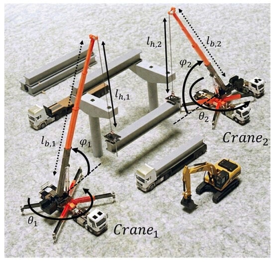
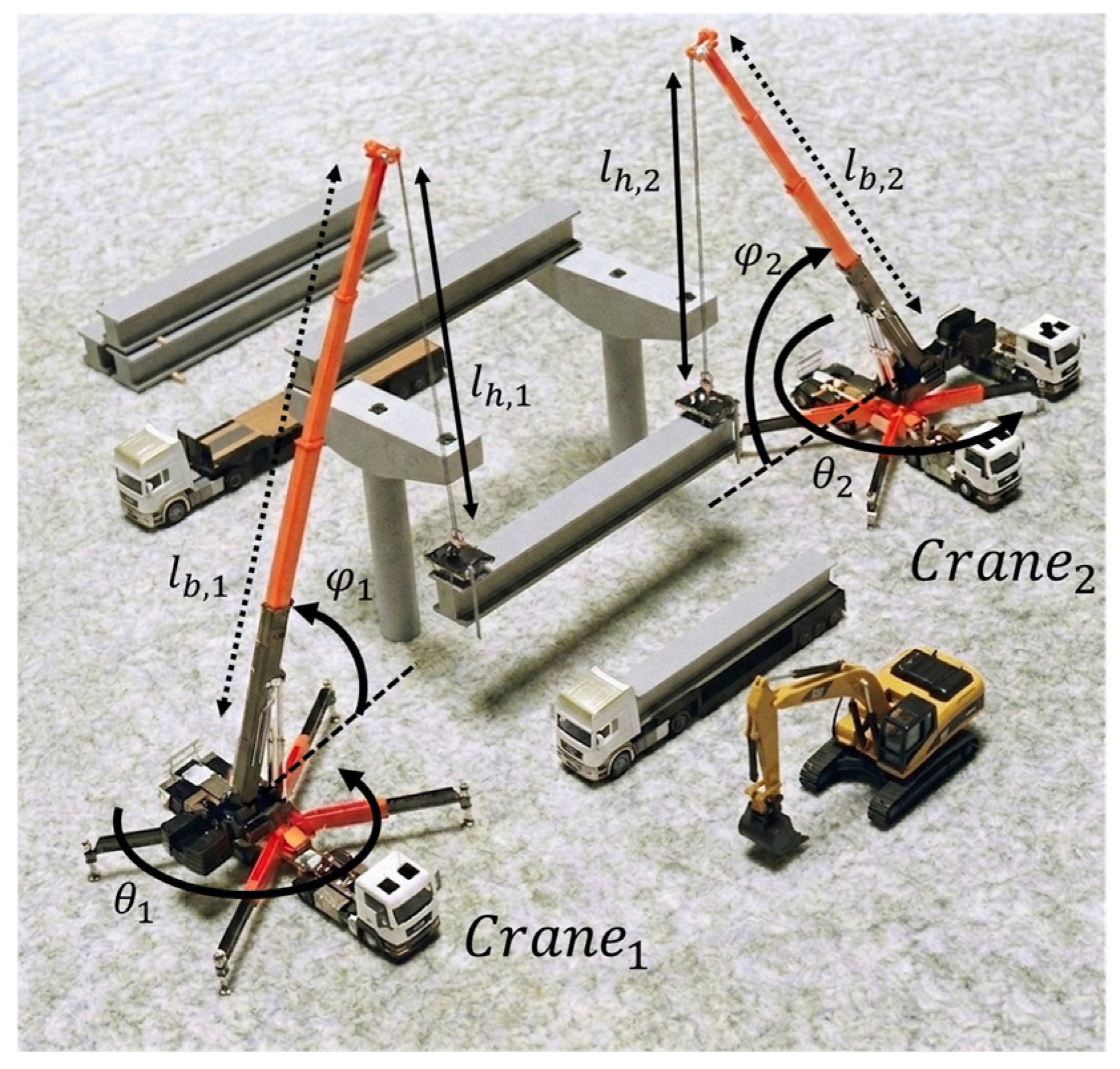
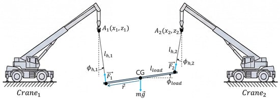
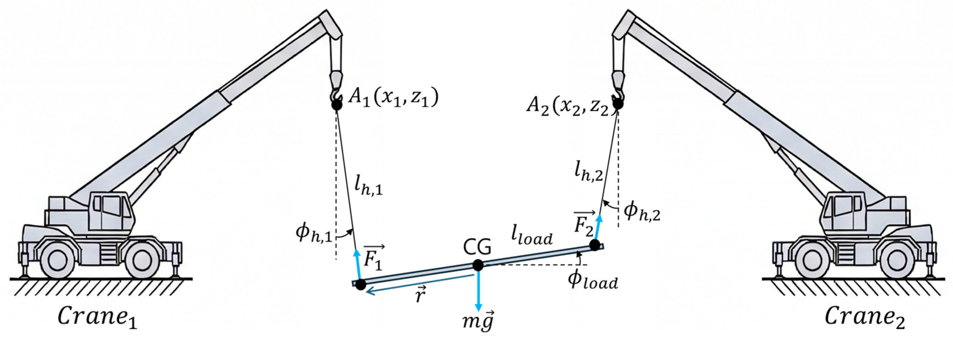
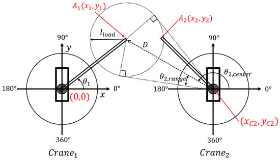
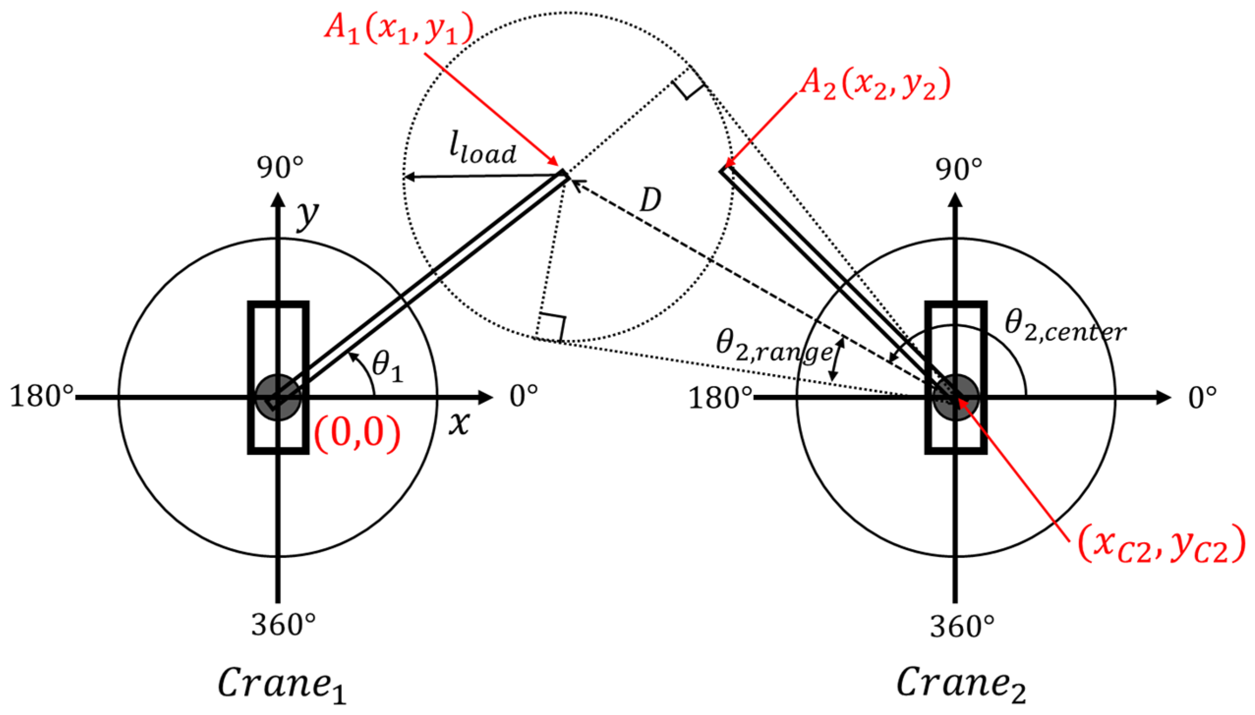
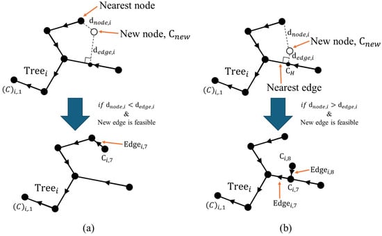
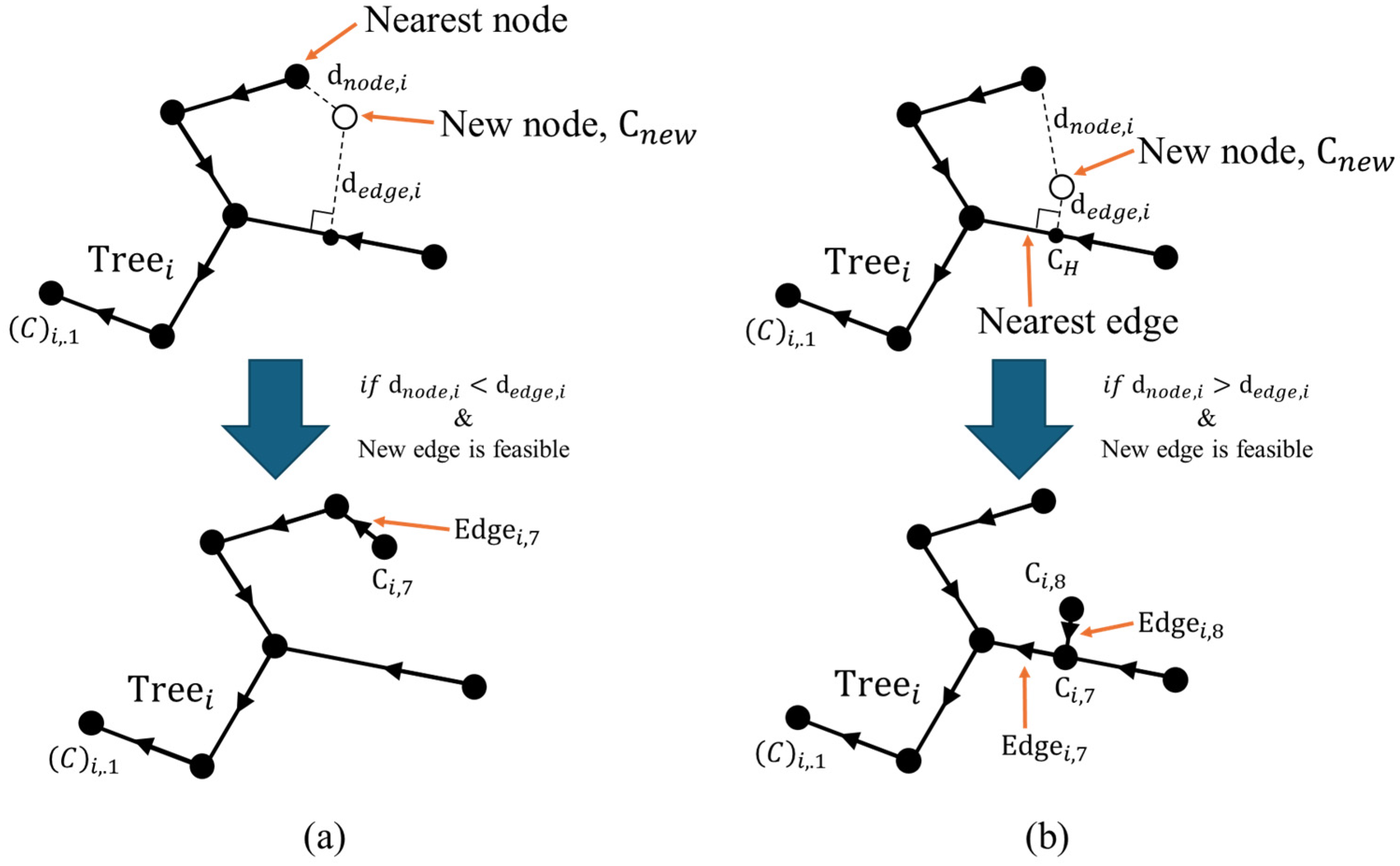
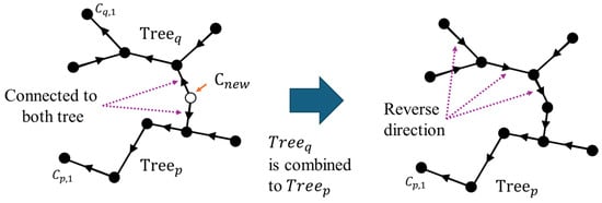
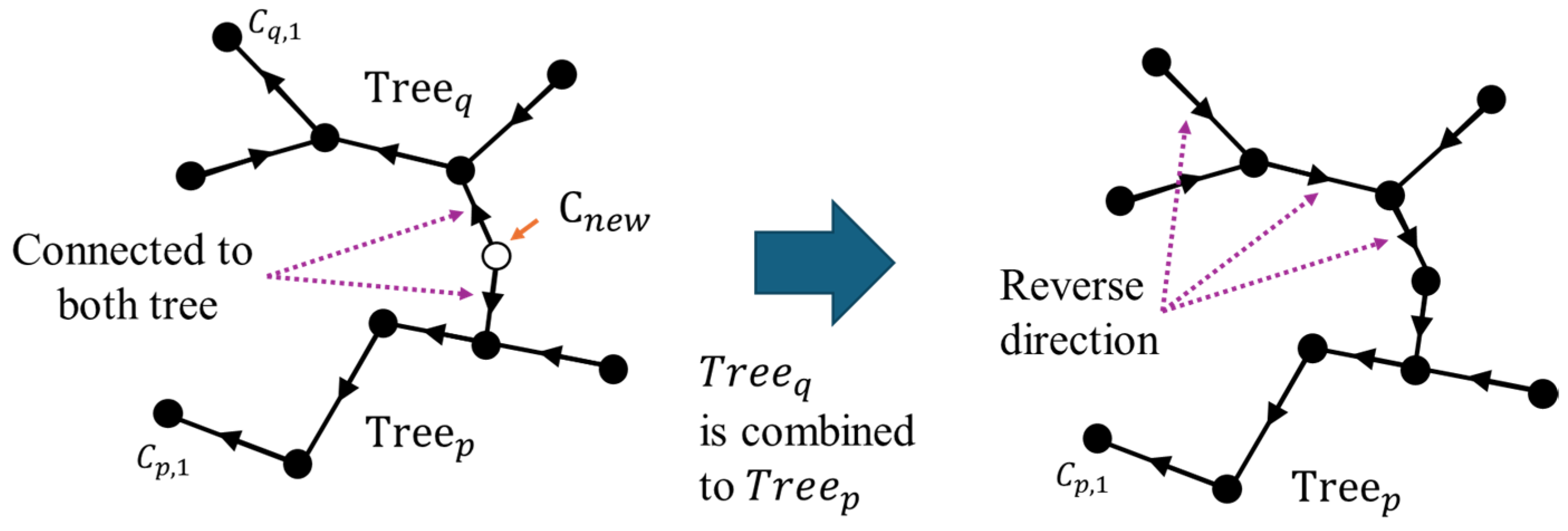
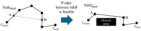
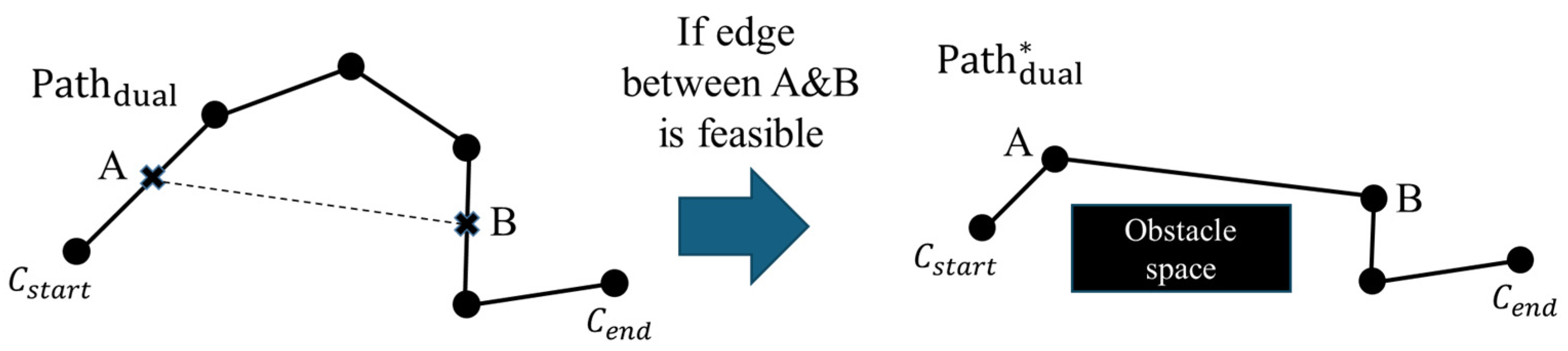
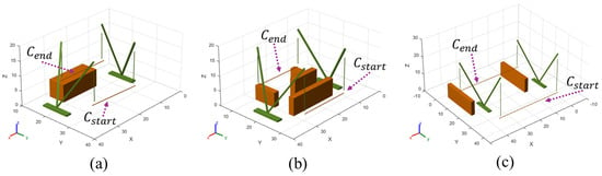
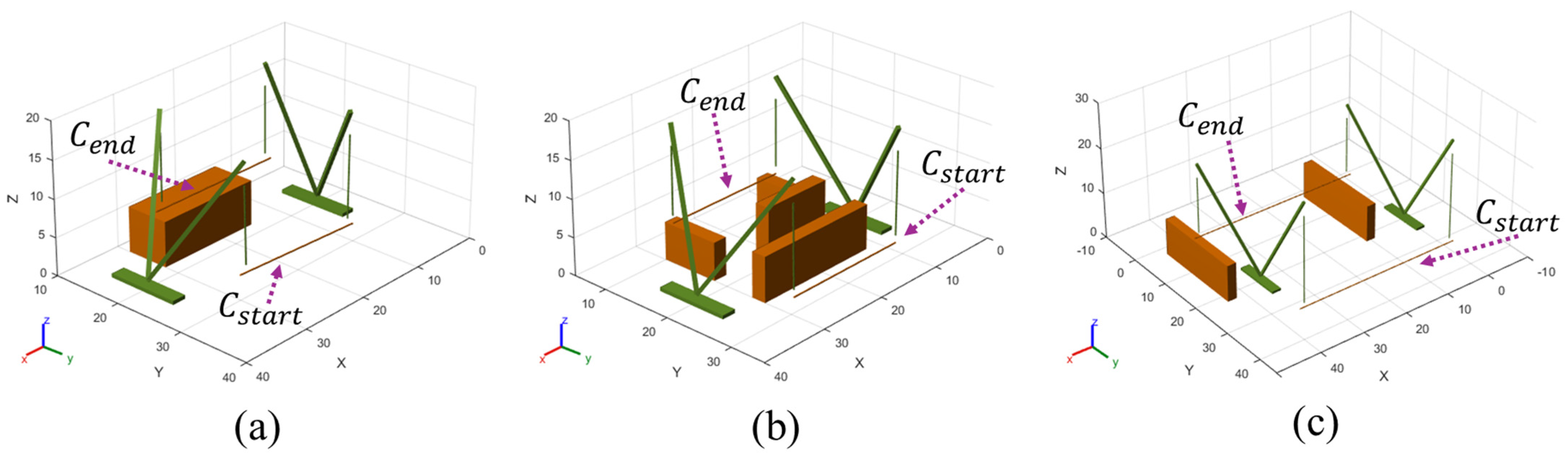
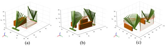
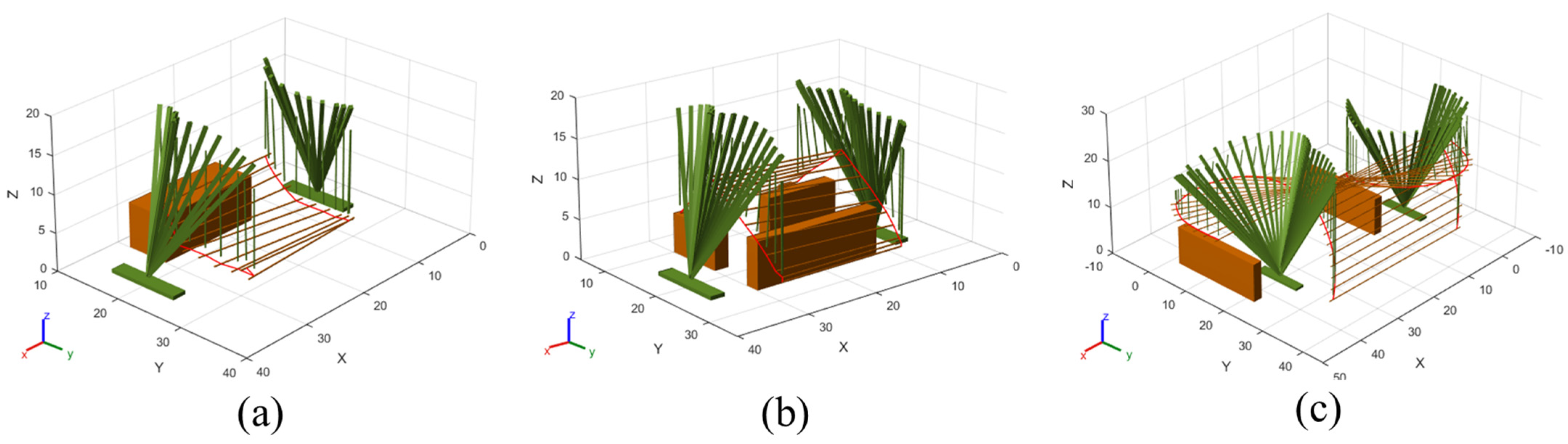
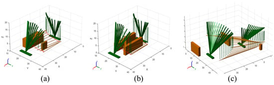
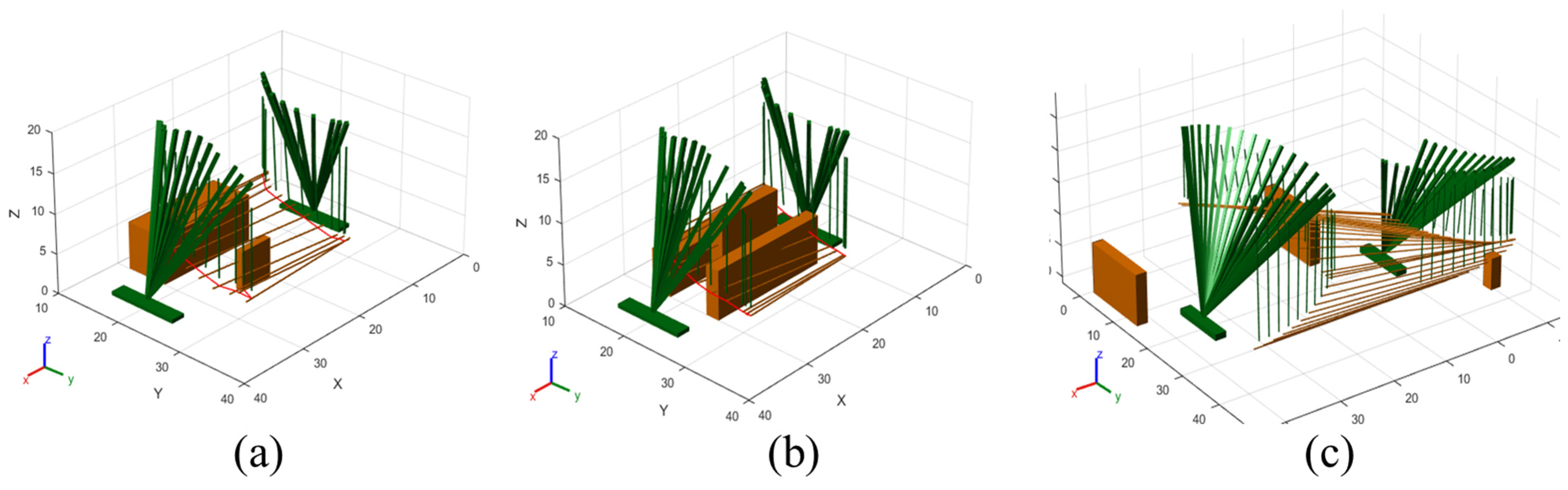
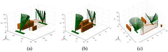
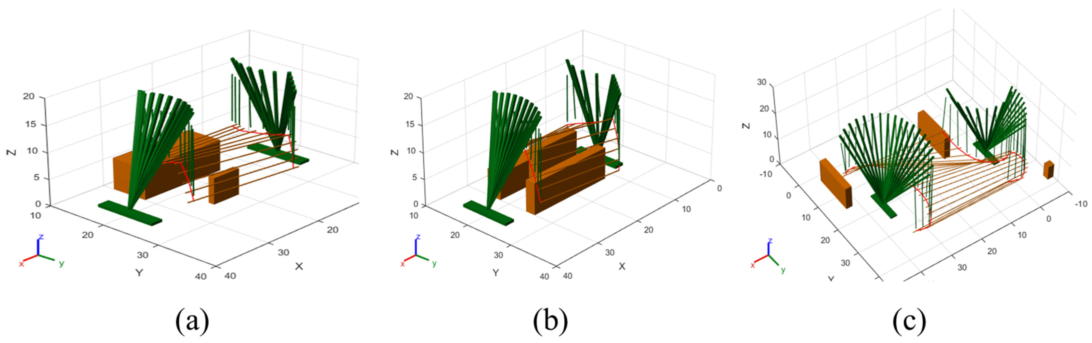
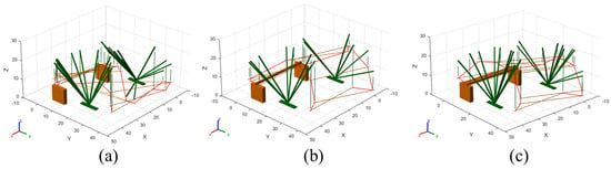
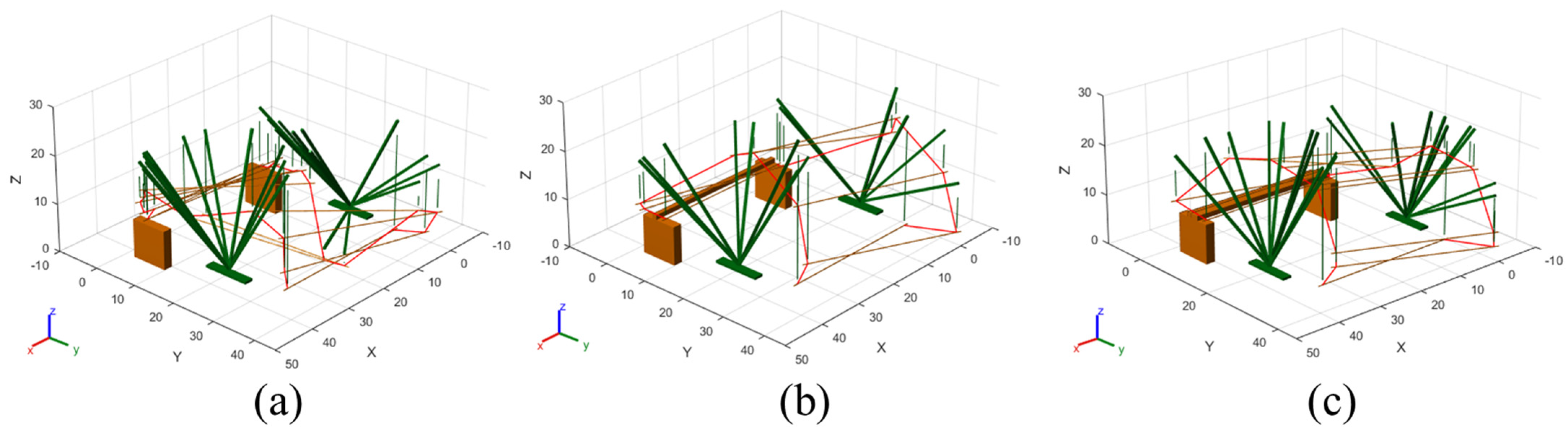

Disclaimer/Publisher’s Note: The statements, opinions and data contained in all publications are solely those of the individual author(s) and contributor(s) and not of MDPI and/or the editor(s). MDPI and/or the editor(s) disclaim responsibility for any injury to people or property resulting from any ideas, methods, instructions or products referred to in the content. |
© 2026 by the authors. Licensee MDPI, Basel, Switzerland. This article is an open access article distributed under the terms and conditions of the Creative Commons Attribution (CC BY) license.