Surrogate-Assisted Multiobjective Optimization of Electric Vehicle Frontal Crashworthiness via Response-Gated Residual Compensation and Uncertainty Calibration

Abstract

High-dimensional mixed variables, strongly nonlinear responses, and unreliable decisions near constraint boundaries remain major challenges in frontal crash optimization of electric vehicles. This study develops a response-gated error-compensated surrogate model (RGEC-SM) and an uncertainty-constrained surrogate-assisted optimization method (UC-SB-NSGA-II) for the 100% frontal rigid-barrier impact of an electric sport utility vehicle. RGEC-SM uses a shared encoder with response-specific feature gates to represent multi-response mappings and applies out-of-fold residual radial-basis-function compensation to responses with stable local bias. Bootstrap ensemble standard deviations are converted, through an independent calibration set, into one-sided conservative prediction bounds for baseline-referenced safety constraint screening. On an independent test set, RGEC-SM achieved R² values of 81.74–91.86% for 13 responses, with a mean NRMSE of 13.4% and a Boundary-NRMSE of 19.4% for safety responses. After conservative constraints were constructed to target 90% one-sided pooled marginal coverage, the false-acceptance rate in the candidate FE audit decreased from 27% to 10.3%, while acceptance precision increased from 73.0% to 89.7%. Under a fixed surrogate-evaluation budget, UC-SB-NSGA-II maintained a conservative-feasible hypervolume comparable to that of NSGA-II, but increased the final-generation conservative baseline-referenced feasible ratio from 48.7% to 79.6%. FE re-simulation of the TOPSIS-selected candidate confirmed that all 11 safety responses were no worse than the baseline design. Body mass decreased from 438.6 kg to 420.4 kg, and vehicle acceleration decreased from 39.4 m/s² to 36.9 m/s², corresponding to improvements of 4.15% and 6.35%, respectively. The proposed method reduces the risk of falsely classifying practically infeasible designs as feasible during surrogate-based optimization.

1. Introduction

The substantial mass of traction batteries and the limited front-end deformation space of electric vehicles place stringent demands on frontal crashworthiness. Under frontal impact, load-bearing structures, including front rails and crash boxes, must absorb impact energy while limiting deformation transmission to the passenger compartment. Lightweighting further intensifies the trade-offs among structural mass reduction, occupant-compartment integrity, and acceleration-pulse control. Previous studies have established foundations in structural crashworthiness optimization [1,2,3,4], response-surface-assisted design [5,6], full-vehicle crash simulation [7,8,9,10], and battery-pack surrogate modeling [2,11]. However, collaborative optimization of high-dimensional mixed variables in full-vehicle frontal crash remains constrained by high computational costs, strong response coupling, and uncertain safety-constraint boundary decisions.

Explicit finite element (FE) analysis can represent nonlinear processes such as material plasticity, contact, buckling, and failure, and is therefore a key tool for frontal-crash performance assessment. However, a single full-vehicle simulation is time-consuming and cannot be embedded directly in evolutionary optimization. Design-of-experiments methods, such as Latin hypercube sampling, have therefore been used to improve sample coverage [12,13], while surrogate models, including response surfaces, Kriging, and radial basis functions, have supported the approximation of nonlinear crash responses [14,15,16,17,18,19,20,21]. Surrogate-assisted evolutionary optimization methods have also shown application potential [11,22,23]. In high-dimensional mixed-variable spaces, however, samples remain sparse, requiring surrogate models to provide both global predictive accuracy and robustness near constraint boundaries.

Existing surrogate models have distinct limitations. The generalization of RBF models depends on kernel-width selection [21,24], Kriging can be computationally expensive for high-dimensional multi-response problems [13,19,20], and BP neural networks are prone to overfitting when the sample size is small [25,26,27]. Model selection is often supported by cross-validation, robust losses, and bootstrap methods [28,29,30,31,32,33]. Crash responses are heterogeneous: the same structural variable may simultaneously improve energy absorption and increase acceleration peaks. Multi-task learning, ensemble learning, and calibrated uncertainty estimation provide useful references for coupled multi-response modeling [34,35,36,37], while feature modulation and variable-importance analysis can support input scaling and engineering interpretation [38, 39,40,41,42]. Nevertheless, these ideas require engineering adaptation to crashworthiness constraint boundaries.

Multiobjective evolutionary algorithms such as NSGA-II are widely used in engineering optimization [43,44,45]. Conventional surrogate-assisted optimization, however, has difficulty distinguishing prediction risk. When the surrogate model exhibits systematic bias in sparse regions or near constraint boundaries, the population can be attracted to falsely advantageous solutions.

Using only fixed penalty functions for safety-related constraints such as intrusion and local deformation, or handling objective responses such as acceleration without distinguishing prediction risk, may lead to feasibility misclassification and search instability [46,47,48,49]. Engineering design screening also requires trade-offs among mass, acceleration, and constraint margins; methods such as TOPSIS and entropy weighting can support post-processing of Pareto solution sets [50,51,52, 53].

To address these issues, this study builds on an existing full-vehicle frontal crash FE model, a 68-dimensional mixed design space, and 600 simulation samples. A response-gated error-compensated surrogate model (RGEC-SM) is proposed. The model uses response-dependent feature gates to identify sensitive parameters, trains RBF compensators on out-of-fold cross-validation residuals for conditional correction, and uses bootstrap ensemble standard deviations to characterize model disagreement. An uncertainty-constrained surrogate-assisted NSGA-II (UC-SB-NSGA-II) is then developed. A one-sided risk multiplier is determined from an independent calibration set and combined with conservative constraint dominance, mixed-variable evolutionary operators, TOPSIS post-processing, and FE re-simulation validation. The objective is to establish a credible surrogate-optimization workflow for high-dimensional, strongly nonlinear, multi-constraint full-vehicle frontal crash problems under a limited simulation budget.

2. Frontal Crash Finite Element Model and Optimization Problem Definition

2.1. Finite Element Model of the Electric Vehicle Frontal Crash

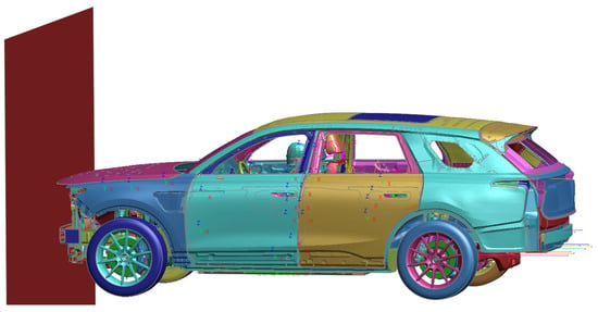
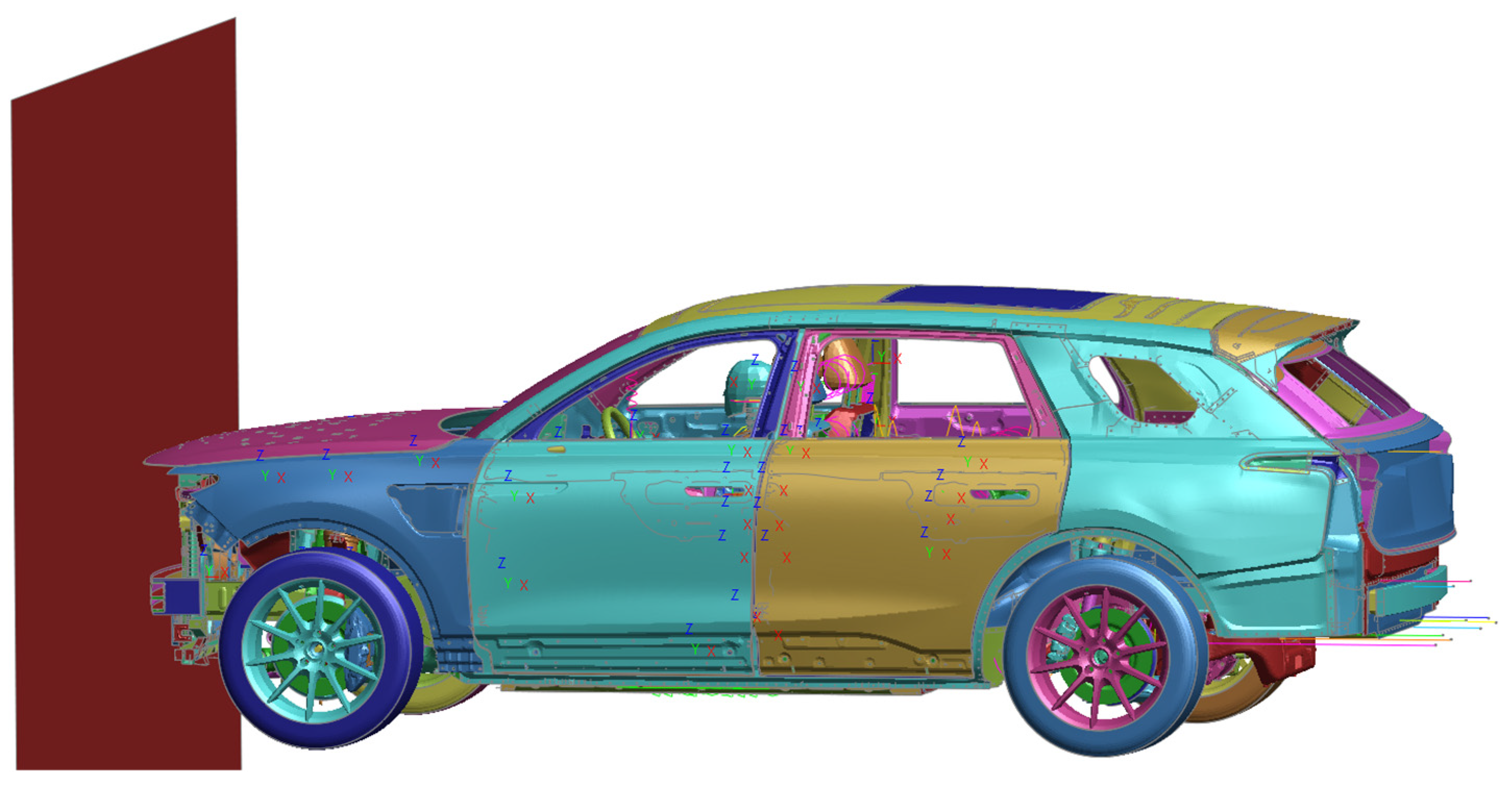
A frontal 100% rigid-barrier impact simulation model was developed for an electric sport utility vehicle according to the 2024 C-NCAP protocol (Figure 1). The main body structure was discretized with shell elements with an average size of approximately 8 mm. The model contained approximately 845,000 nodes and 830,000 elements. The material set included representative body metals, including low-strength steel, high-strength steel, advanced high-strength steel, and aluminum alloys. LS-DYNA Material Model 24 was used to describe elastoplastic behavior; the stress-strain curves were mainly obtained from test data and included strain-rate effects and dynamic hardening. Connections were represented by solid spot-weld and solid adhesive elements, while spot-weld failure was not considered. Contacts included body self-contact and body-to-rigid-wall surface contact, with friction coefficients of 0.1 and 0.2, respectively. The vehicle impacted the rigid barrier at 55 km/h, and the simulation termination time was 0.12 s.

Figure 1. Boundary conditions for the body structure under the frontal crash condition.

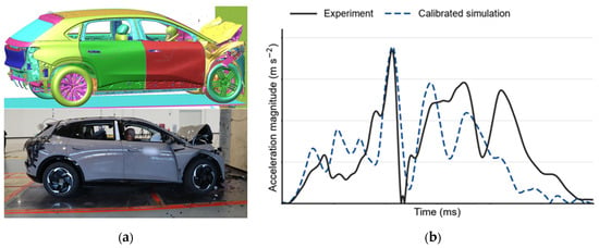
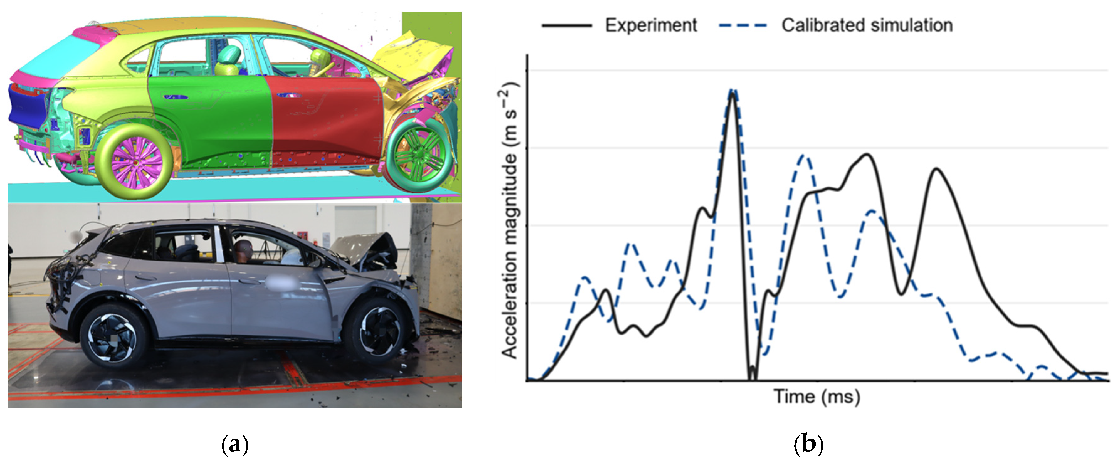
Figure 2a shows that the calibrated FE model reproduces the principal front-end crush mode and overall vehicle deformation observed in the full-vehicle rigid-barrier test. In Figure 2b, the simulated acceleration captures the dominant deceleration pulse and the overall multi-peak trend, although local deviations remain during the early and middle response phases. The agreement in deformation mode and acceleration response establishes the baseline FE model as the reference for subsequent parametric optimization. Throughout the optimization, the impact conditions, contact treatment, and constitutive modeling framework were retained, while structural geometry, component positions, thicknesses, and material assignments were varied within the prescribed design ranges.

Figure 2. Validation of the baseline frontal crash FE model against the full-vehicle rigid-barrier test: (a) deformation comparison; (b) acceleration time-history comparison.

2.2. Design Variables for Frontal Crashworthiness Optimization

Based on frontal-crash load transfer paths, local intrusion-sensitive regions, and the parametric modeling requirements of the SFE concept, the main variable regions were defined around key load-bearing structures, including the B-pillar, longitudinal members, A-pillar, dash cross member, upper rail, seat cross member, and floor. Representative geometric/positional input variables are listed in Table 1. The initial design-variable combination was denoted as the baseline design and consisted of the initial geometric/positional parameters and the initial material-thickness configuration of the current body model. The FE responses of this initial design under frontal crash conditions were used as performance boundaries for subsequent baseline-referenced constraints.

Table 1. Representative geometric and positional input variables.

Order	Input Variable	Initial	Range	Illustration
1	VIR/G/LON-F/X	277	[−50, 50]
2	VIR/G/LON-R/Z	158.4	[−10, 10]
3	VIR/G/SHOTGUN-F/Z	32.2	[−10, 10]
4	VIR/G/TUNNEL/Z	50.5	[−5, 15]
5	VIR/G/ROCKER/Z	87.5	[−5, 5]
6	VIR/G/ROOF-SIDE-RAIL/Z	116.3	[−10, 10]
7	VIR/G/BPILLAR-Lower/X	248.2	[−10, 10]
8	VIR/G/BPILLAR-Lower/Y	81.2	[0, 10]
9	VIR/G/BPILLAR-Middle/X	207.6	[−10, 10]
10	VIR/G/BPILLAR-Middle/Y	75.4	[0, 10]
11	VIR/G/BPILLAR-Upper/X	159.8	[−10, 10]
12	VIR/G/BPILLAR-Upper/Y	32.2	[0, 10]
…	…	…	…	…
32	VIR/G/R-Roof-Side-Rail/Y	88	[0, 10]

Note: “…” indicates that other geometric and positional input variables are omitted for brevity.

The thickness/material variables describe the material-thickness combinations of key load-bearing components. Each variable can take values only from a predefined candidate set. For each discrete variable, a candidate index is assigned, and the corresponding material grade, thickness, and related FE material-card parameters are determined by a predefined mapping table. The candidate index is used only for discrete selection during optimization and FE model generation and is not directly treated as a continuous numerical input to the surrogate model.

Accordingly, the original design space for the frontal rigid-barrier (FRB) condition comprised 32 continuous geometric/positional variables and 36 discrete material-thickness variables, resulting in 68 design decision variables in total (Table 2). The continuous variables were normalized, while each discrete variable, containing three candidate categories, was represented using one-hot encoding, yielding an encoded input dimension of 140 for the surrogate model.

Table 2. Details of the input variables.

Variable Group	Num.	Description	Type	Encoding Method	Related Structure
Geometric/position variables	32	Spatial dimensions or relative positions of key structural regions	Continuous	Physical bounds	B-pillar, rocker, upper rail, seat cross member, dog-leg region
Thickness/material variables	36	Thickness and material assignment of load-bearing panels and reinforcements	Discrete	Candidate ID; one-hot categorical encoding; material–thickness mapping for FE model generation	B-pillar reinforcement, rocker, rail, floor, cross member
Encoded ML features	din	Numerical representation after continuous-variable normalization and categorical encoding	Mixed	Normalized feature vector	x = Φ(z)

Latin hypercube sampling (LHS) was employed to generate 600 FE samples, utilizing its stratified space-filling properties to promote broad coverage of the prescribed design-variable ranges under the limited simulation budget. Among the 390 training samples, 1027 sample–response pairs were identified near the predefined boundaries of the 11 safety constraints, including 541 on the feasible side and 486 on the infeasible side.

2.3. Crashworthiness Responses and Baseline-Referenced Performance Constraints

After the batch FE simulations, the FRB crash time histories were converted into scalar response labels suitable for surrogate-model training. The selected outputs mainly included front-floor intrusion, front-door intrusion, accelerator-pedal intrusion, dash deformation, vehicle acceleration, and body mass (Table 3). Displacement and intrusion responses characterize occupant-compartment retention, enabling the resulting dataset to support both crashworthiness prediction and subsequent multiobjective optimization.

Table 3. Output responses.

Response Group	Suggested Symbol	Response Group	Suggested Symbol
Front floor intrusion	$u_{\mathit{FF},k}^X(k=1,2,3,4)$	Accelerator pedal intrusion	$u_{\mathit{AP}}^X, u_{\mathit{AP}}^Z$
Front-door intrusion	$u_{\mathit{FD},k}^X(k=1,2,3,4)$	Maximum front-end deformation	$u_{\mathit{MFE}}^X$
Body mass	m	Vehicle acceleration	a

For the investigated 100% frontal rigid-barrier impact condition, the selected responses primarily focus on vehicle body mass, acceleration, and structural intrusion or local deformation. Although frontal impact loads may propagate toward the battery pack region through the surrounding structures, battery-specific responses were not included in the present optimization framework, and battery safety was therefore not directly evaluated.

Continuous geometric/positional variables and output responses were normalized using Equation (1). Discrete material-thickness variables were not numerically normalized by candidate index, but were first converted into categorical encodings according to the candidate mapping table. Binary one-hot features retained their 0/1 values and were not normalized again.

$$x_{\mathit{norm}}=-1+2{\displaystyle \frac{x-x_{\mathit{low}}}{x_{\mathit{high}}-x_{\mathit{low}}}}$$

(1)

where the original variable, its lower and upper bounds, and the normalized value mapped to the interval [−1, 1] are defined as in Equation (1).

3. Methodology

3.1. Uncertainty-Aware Multi-Response Surrogate Model

3.1.1. Overall Model Architecture

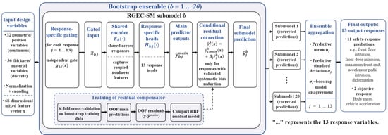
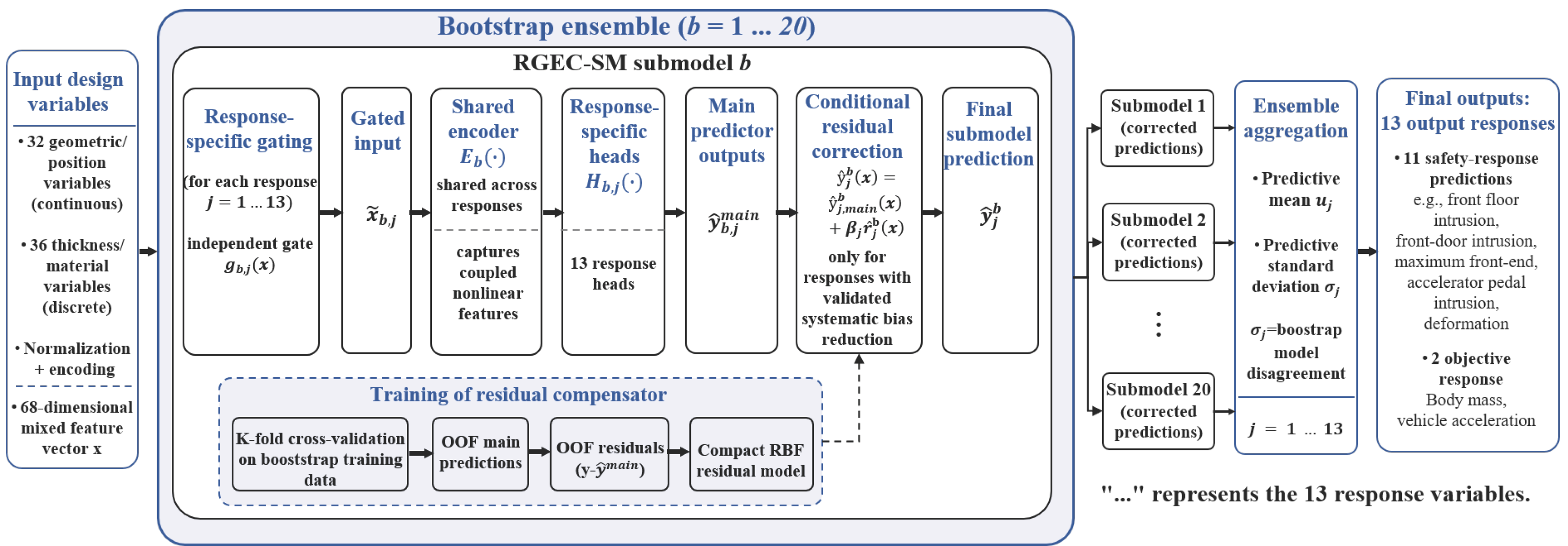
As shown in Figure 3, a response-gated error-compensated surrogate model (RGEC-SM) was constructed to describe the nonlinear relationship between the encoded input features derived from the original mixed design variables and the 13 output responses. The 13 outputs included body mass, vehicle acceleration, and 11 safety-related intrusion or local-deformation responses. Body mass and vehicle acceleration were used as optimization objectives; the remaining 11 responses were converted into risk measures for baseline-referenced non-degradation constraint decisions.

Figure 3. Overall architecture and training-inference workflow of RGEC-SM.

RGEC-SM consists of multiple bootstrap submodels. Training samples for each submodel are obtained by resampling the training set with replacement. The network topology is identical across submodels, but the parameters are independent. In each submodel, every output response has an independent feature gate and output head, while the encoder is shared by all 13 response branches. This architecture preserves the response-specific dependence on input variables while exploiting nonlinear representations shared across responses.

To address possible local systematic bias in the main predictor, compact RBF compensators were trained using out-of-fold residuals. Whether residual compensation was enabled was determined on the validation set and controlled by a response-level binary switch; this switch was kept identical across all bootstrap submodels. The ensemble layer finally outputs the prediction mean and standard deviation. The mean is used for response prediction and objective evaluation, while the standard deviation characterizes model disagreement and is subsequently calibrated for safety constraint construction.

3.1.2. Response-Dependent Feature Gating

For the corresponding output response in each submodel, feature-wise sigmoid gates were applied to the encoded input features. The gating, input modulation, and main prediction process are written as follows:

$$g_j^b\left(x\right)=\sigma \left(f_{\mathit{gate},j}^b\left(x\right)\right)$$

(2)

$${\tilde{x}}_j^b=x\odot \left[1+\eta \left(2g_j^b\left(x\right)-1\right)\right],\eta =0.5$$

(3)

$${\hat{\mathrm{y}}}_{j,\mathit{main}}^b\left(x\right)=h_j^b\left(E^b\left({\tilde{x}}_j^b\right)\right)$$

(4)

where the gating network, shared encoder, and response-specific output head are defined in Equations (2)–(4). The feature scaling coefficients lie between 0.5 and 1.5, preventing weakly sensitive features from being completely suppressed.

The gate values reflect only the model’s tendency to modulate input features. They do not directly represent causal contributions or true load-path weights. Subsequent engineering interpretation combines group permutation importance with FE perturbation sensitivity. For one-hot encoded material-thickness variables, the corresponding encoded columns are treated as original variable groups.

3.1.3. Conditional Residual Compensation

The RBF compensator used the out-of-fold residuals of the main predictor as supervised signals. For each bootstrap submodel, its bootstrap training set was partitioned by original sample ID; repeated copies of the same original sample were always assigned to the same fold. After the main prediction was generated for the held-out fold, the out-of-fold residual for each sample and response was defined as follows:

$$e_{i,j}^{\mathrm{b},\mathrm{OOF}}=y_{i,j}^{\mathrm{std}}-{\widehat{y}}_{j,\mathrm{main}}^{\mathrm{b},\mathrm{OOF}\left(x_i\right)}$$

(5)

The RBF compensator corresponding to each response was trained using all out-of-fold sample pairs. The main predictor was then retrained on the complete bootstrap training set, and the final prediction was written as follows:

$$y_j^b\left(x\right)=y_{j,\mathrm{main}}^b\left(x\right)+{\beta }_j{r}_j^b\left(x\right),{\beta }_j\in \left\{0,1\right\}$$

(6)

where the response-level switch does not change with the submodel index. For the 11 baseline-referenced constraint responses, compensation was enabled only when the compensated validation-set NRMSE satisfied the predefined improvement requirement, and the Boundary-NRMSE relative to the corresponding baseline-referenced boundary did not deteriorate. For mass and vehicle acceleration, compensation was enabled according only to validation-set NRMSE. All compensation criteria were fixed before training. The sample-ID-grouped OOF procedure prevents duplicated bootstrap observations from entering both fitting and held-out folds, while validation-based activation limits corrections that fail to generalize beyond the training data.

3.1.4. Training Objective and Uncertainty Estimation

The main predictor was trained in the standardized output space. The loss of each submodel consisted of a Huber fitting term, an L2 parameter-regularization term, and a gate negative-entropy term:

$${\mathcal{L}}_{\mathrm{main}}^{\left(b\right)}={\displaystyle \frac{1}{n_{b}J}}{\sum }_{i=1}^{n_b}{\sum }_{j=1}^J{\rho }_{\delta }[y_{i,j}^{\mathrm{std}}-{}^{^}y_{j,\mathrm{main}}^{\left(b\right)}\left({\mathbf{x}}_i\right)]+{\lambda }_w{\left||{\Theta }_{\mathrm{main}}^{\left(b\right)}|\right|}_2^2+{\lambda }_g{\mathcal{R}}_{\mathrm{gate}}^{\left(b\right)}$$

(7)

where the parameter set includes the gating network, shared encoder, and output heads, and the negative-entropy term is computed from the gate values. This term suppresses premature gate saturation to 0 or 1. All output responses were trained with equal weights in the standardized space.

After inverse standardization, the final predictions of the submodels were ensembled in engineering units:

$${\mu }_j\left(x\right)=1/B{\sum }_{b=1}^B{\hat{\mathrm{y}}}_{j,\mathit{phy}}^{\left(b\right)}\left(x\right)$$

(8)

$${\sigma }_j\left(x\right)={\left[1/\left(B-1\right){\sum }_{b=1}^B{\left({\hat{\mathrm{y}}}_{j,\mathit{phy}}^{\left(b\right)}\left(x\right)-{\mu }_j\left(x\right)\right)}^2\right]}^{1/2}$$

(9)

where the ensemble mean is used for response prediction and subsequent objective function evaluation, and the ensemble standard deviation characterizes prediction disagreement among bootstrap submodels. It is not interpreted as a strict probabilistic confidence interval. Its calibration and use in conservative constraints are described in Section 3.2.

3.1.5. Model Training and Evaluation

Before bootstrap resampling, the 600 FE samples were split by original sample ID into training, validation, calibration, and final test sets at a ratio of 65%/15%/10%/10%. The training set was used for hyperparameter determination, model training, and construction of residual compensators. The validation set was used for early stopping and determining the compensation switch. The calibration set was used only to estimate the safety constraint risk multiplier, while the test set was used only for final accuracy and feasibility-decision evaluation.

Continuous geometric/positional variables were normalized according to their physical bounds, and discrete material-thickness variables were encoded using variable-specific one-hot representations. Standardization parameters for the output responses were calculated only from the original training set and kept fixed for all data subsets and bootstrap submodels. The RGEC-SM network and residual-compensation RBF hyperparameters were determined through cross-validation within the training set and then fixed for all bootstrap submodels.

The shared encoder consisted of two ReLU layers with 64 units each. Each output response was assigned a response-specific output head with one hidden layer of 32 units. The gate bottleneck dimension was fixed. The number of RBF centers was selected from the candidate set; centers were determined by K-means, and the kernel width was initialized according to the median distance between centers. The main predictor used validation-set NRMSE for early stopping and restored the best weights when no improvement was observed for 50 consecutive epochs. The bootstrap ensemble size was set to B = 20, balancing prediction stability and computational cost.

For comparison, RBF, Kriging, and BP models were constructed using the same data partitioning as RGEC-SM. The RBF model employed Gaussian basis functions with 80 centers determined by K-means clustering, and the kernel width was set to the median distance between centers. Kriging adopted a Gaussian correlation function and a constant trend, with correlation parameters estimated by maximum likelihood. Both RBF and Kriging were fitted independently for the 13 responses. The BP model employed two hidden layers with 64 and 32 ReLU neurons, respectively, and a 13-dimensional output layer. It was trained using Adam with a learning rate of 0.001 and L2 regularization of 10⁻⁴, with early stopping based on validation performance.

Model accuracy was evaluated using R2 and NRMSE. For the 11 safety responses, Boundary-NRMSE was further evaluated near the constraint threshold. Let the initial baseline risk upper bound and the predefined boundary bandwidth be defined for each safety-related response; then:

$${\mathcal{B}}_j=\left\{\mathbf{x}:\left|q_j^{\mathrm{FE}}\left(\mathbf{x}\right)-q_j^{\mathrm{base}}\right|\le {\Delta }_j=\rho R_{j,\mathit{train}}\right\}$$

(10)

$${\mathrm{Boundary}-\mathrm{NRMSE}}_j={\displaystyle \frac{\sqrt{\frac{1}{\left|{\mathcal{B}}_j\right|}\sum _{\mathbf{x}\in {\mathcal{B}}_j}{\left[{\widehat{q}}_j\left(\mathbf{x}\right)-q_j^{\mathrm{FE}}\left(\mathbf{x}\right)\right]}^2}}{R_{j,\mathrm{train}}}}\times 100\%$$

(11)

where the response range in the original training set and the fixed boundary-bandwidth ratio are defined as in Equations (10) and (11). Boundary-NRMSE was used only for the 11 safety responses; mass and vehicle acceleration were reported using R2 and NRMSE only.

3.2. Surrogate-Assisted Multiobjective Optimization with Uncertainty-Based Conservative Constraints

3.2.1. Mathematical Formulation of the Multiobjective Optimization Problem

Let the original mixed design vector contain 68 decision variables. The feasible set satisfies both continuous-variable bounds and discrete candidate sets. Evolutionary operations are performed directly in the original mixed-variable space, and surrogate-model inputs are obtained through the encoding procedure.

The objectives are to minimize body mass and vehicle acceleration:

$$\begin{array}{l}\underset{\mathbf{x}\in \mathsf{\Omega }}{\min }\left[m\left(\mathbf{x}\right),a\left(\mathbf{x}\right)\right]\\ q_j\left(\mathbf{x}\right)=-y_j\left(\mathbf{x}\right)\\ q_j\left(\mathbf{x}\right)\le q_j^{\mathrm{base}},\hspace{1em}j=1,\dots ,11\end{array}$$

(12)

All 11 safety responses are negative displacement or intrusion quantities; values closer to 0 indicate better safety performance. Therefore, sign reversal was used to convert them into upper-bound risk constraints. These constraints require each candidate design to be no worse than the initial baseline design for every safety-related response. The true FE risk values are used only for calibration, testing, and final re-simulation verification.

3.2.2. Conservative Constraint Dominance and Candidate Screening for Non-Objective Responses

The 11 safety-related responses were converted into positive risk measures, and the risk value of the initial baseline design was defined as the baseline-referenced upper bound for each response. For any candidate design, RGEC-SM outputs the predicted risk mean and bootstrap ensemble standard deviation. To avoid incorrectly retaining candidates whose actual performance is worse than the initial baseline design when only the prediction mean is used, nominal and conservative baseline-referenced constraints were defined as follows:

$$\left\{\begin{array}{c}{\widehat{q}}_j\left(\mathbf{x}\right)\le q_j^{\mathrm{base}}\\ {\widehat{q}}_j\left(\mathbf{x}\right)+k{\sigma }_j\left(\mathbf{x}\right)\le q_j^{\mathrm{base}}\end{array}\right.\mathit{j}=1,\dots ,11$$

(13)

The nominal constraint is used only to identify candidates that may be no worse than the baseline according to surrogate predictions. The conservative constraint is used for actual screening during optimization. A candidate satisfying all 11 conservative constraints is considered to maintain predicted performance no worse than the initial baseline after accounting for surrogate-model disagreement.

The global risk multiplier k, which scales the bootstrap ensemble standard deviation in the conservative prediction bound, was determined from an independent calibration set. The smallest multiplier satisfying the 90% one-sided pooled marginal coverage target was selected:

$$k=\underset{\kappa \ge 0}{\min }\left\{\kappa :{\displaystyle \frac{1}{11\left|D_{\mathrm{cal}}\right|}}{\sum }_{{\mathbf{x}}_i\in D_{\mathrm{cal}}}{\displaystyle {\sum }_{j=1}^{11}}\mathbb{I}\left[q_{\mathit{ij}}^{\mathrm{FE}}\le {\widehat{q}}_{\mathit{ij}}+\kappa {\sigma }_{\mathit{ij}}\right]\ge 0.90\right\}$$

(14)

where the FE risk value for each calibration sample and response and the indicator function are defined in Equation (14). The pooled coverage criterion was adopted to calibrate a single global risk multiplier across the 11 safety responses using the available calibration samples. During optimization, each candidate was screened against all 11 conservative constraints simultaneously. The pooled marginal coverage does not establish a 90% joint coverage guarantee; therefore, empirical joint coverage was additionally evaluated on the independent test set as the proportion of designs for which all 11 FE responses fell within their corresponding calibrated upper prediction bounds.

For candidates that failed the conservative constraints, a normalized total violation degree was used for ranking:

$$V\left(\mathbf{x}\right)={\displaystyle {\sum }_{j=1}^{11}}\max \left[0,{\displaystyle \frac{{\widehat{q}}_j\left(\mathbf{x}\right)+k{\sigma }_j\left(\mathbf{x}\right)-q_j^{\mathrm{base}}}{R_{j,\mathrm{train}}}}\right]$$

(15)

where the response range in the original training set is used for normalization. A smaller violation degree indicates that the candidate is closer to satisfying all conservative baseline-referenced constraints.

During environmental selection, UC-SB-NSGA-II first prioritizes candidates that satisfy all conservative baseline-referenced constraints. If two candidates both satisfy all conservative constraints, they are ranked using the non-dominated sorting and crowding-distance criteria of NSGA-II. If both candidates violate the conservative constraints, the candidate with the smaller total violation degree is retained first; if the violation degrees are identical, non-dominated rank and crowding distance are then compared.

Candidates that are nominally baseline-referenced feasible but fail the conservative constraints are defined as the boundary-uncertain candidate set. These candidates indicate that the predicted mean is not worse than that of the initial baseline, but that performance retention cannot be confirmed after considering surrogate-model disagreement. Boundary-uncertain candidates may be used for subsequent FE re-simulation and false-acceptance statistics, but they are not included in final Pareto solution screening or TOPSIS recommendations. After optimization, the non-dominated set is extracted only from conservatively baseline-referenced feasible candidates and used for subsequent multiobjective decision making and FE validation.

In this study, the initial baseline design is used only to define the performance-reference upper bound for each response and is not included as a TOPSIS candidate.

3.2.3. Mixed-Variable Evolutionary Operators and Termination Criteria

SBX crossover and polynomial mutation were used for continuous variables. Uniform crossover of candidate indices and random-reset mutation were used for discrete material-thickness variables. Uniform crossover inherits only legal candidate values from the two parents, while random reset resamples from the candidate set corresponding to the variable. After crossover or mutation, out-of-bound continuous variables are clipped, illegal discrete values are mapped to the corresponding candidate sets, and manufacturing, assembly, and formability constraints are checked. Individuals that cannot be repaired are discarded and regenerated.

The population size and maximum number of generations were set to 100 and 200, respectively, corresponding to a maximum budget of 20,000 surrogate evaluations per run, including the initial population. For continuous variables, the SBX crossover probability and distribution index were set to 0.9 and 15, respectively, while the polynomial mutation probability and distribution index were set to 1/32 and 20, respectively. For discrete variables, uniform crossover and random-reset mutation were employed, with the random-reset probability set to 1/36 per variable. The same population size, evolutionary operator settings, and random-seed groups were used for all comparison algorithms.

The algorithm terminates when the maximum number of generations is reached or when the conservative-feasible hypervolume stagnates. Hypervolume is calculated only from the conservatively baseline-referenced feasible non-dominated set, using the objective-normalization range and reference point fixed before optimization. If no individual satisfies all conservative baseline-referenced constraints in the current generation, HV is set to 0. If the relative HV gain remains below the threshold for 15 consecutive generations, the algorithm stops early; otherwise, it runs to the maximum number of generations. The final conservative feasible non-dominated set is used for subsequent design screening.

3.2.4. Pareto Solution Post-Processing and FE Verification

TOPSIS screening was applied only to the conservatively feasible non-dominated set. For each candidate, three indicators were used: body mass, vehicle acceleration, and the minimum normalized conservative constraint margin:

d_i1 = μ_m(Φ(z_i)), d_i2 = μ_a(Φ(z_i))

(16)

$$M_{\min }\left(\mathbf{x}\right)=\underset{j=1,\dots ,11}{\min }{\displaystyle \frac{q_j^{\mathrm{base}}-\left[{\widehat{q}}_j\left(\mathbf{x}\right)+k{\sigma }_j\left(\mathbf{x}\right)\right]}{R_{j,\mathrm{train}}}}$$

(17)

where body mass and vehicle acceleration are cost indicators, and the minimum normalized conservative margin is a benefit indicator representing the smallest normalized difference between the baseline risk threshold and the conservative prediction bound across the 11 safety responses. The three indicators were converted to a positive Min–Max scale and treated with equal weights. Relative closeness was calculated using the standard TOPSIS procedure, and the design with the highest closeness was selected as the overall recommended candidate.

4. Results and Discussion

4.1. Prediction Accuracy of the Multi-Response Surrogate Model and Baseline-Referenced Constraint-Boundary Discrimination

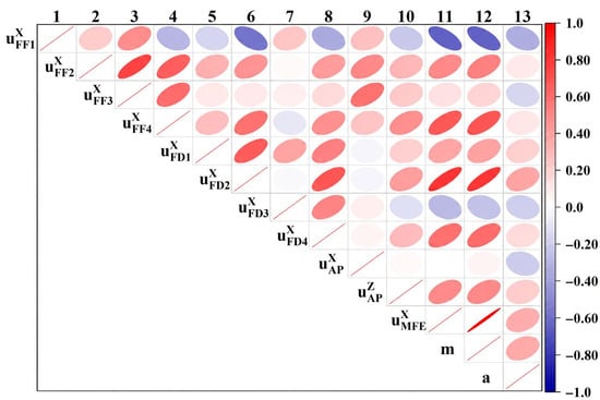
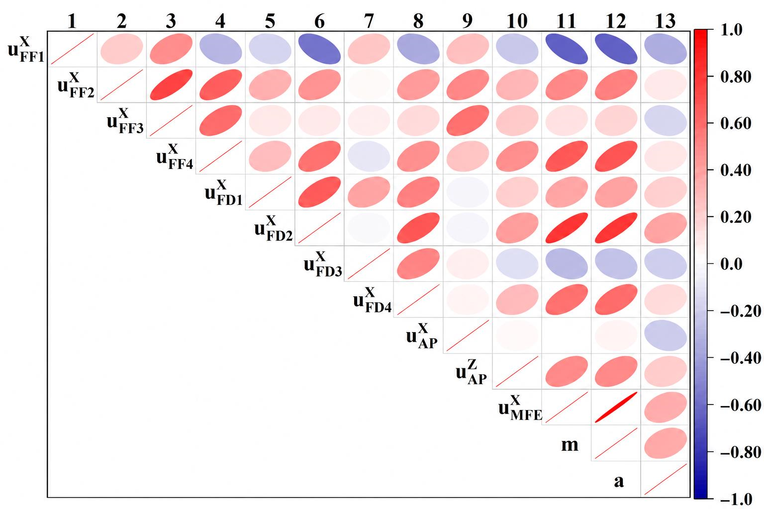
Figure 4 shows the Pearson correlation matrix for the 13 output responses. The 11 intrusion and local-deformation responses exhibit varying degrees of correlation, indicating that they are influenced by partially shared structural parameters and load-transfer paths. At the same time, maximum front-end deformation, body mass, and vehicle acceleration differ from the intrusion responses in both correlation direction and strength. Therefore, it is reasonable to use a shared encoder to extract common multi-response features while retaining response-specific branches for differentiated prediction.

Figure 4. Correlation coefficients among the 13 responses.

Table 4 compares the prediction results of RBF, Kriging, BP, and RGEC-SM on the independent final test set. The R² values of the RBF, Kriging, and BP models were approximately 60.83–73.74%, 64.72–72.87%, and 63.18–72.94%, respectively, indicating limited capability to represent multi-response nonlinear relationships under high-dimensional mixed design variables. RGEC-SM achieved R2 values of 81.74–91.86% across the 13 responses, with an average of 86.69%; its NRMSE ranged from 10.5% to 17.6%, with an average of 13.4%. Compared with the three baseline models, RGEC-SM provided higher prediction consistency for intrusion, local deformation, body mass, and vehicle acceleration.

Table 4. Response-wise comparison of different surrogate models.

	RBF		Kriging		BP		RGEC-SM
	R2	NRMSE	R2	NRMSE	R2	NRMSE	R2	NRMSE
$u_{\mathit{FF}1}^X$	67.84%	23.4%	71.23%	22.2%	65.41%	24.2%	86.72%	15.9%
$u_{\mathit{FF}2}^X$	64.36%	23.2%	68.91%	21.7%	72.17%	20.6%	84.58%	16.4%
$u_{\mathit{FF}3}^X$	69.72%	23.3%	66.43%	24.5%	63.18%	25.5%	87.94%	15.5%
$u_{\mathit{FF}4}^X$	67.26%	22.6%	72.87%	20.7%	68.34%	22.2%	82.63%	17.6%
$u_{\mathit{FD}1}^X$	70.83%	15.6%	65.27%	17.0%	68.94%	16.1%	85.71%	12.7%
$u_{\mathit{FD}2}^X$	62.74%	20.5%	67.86%	19.1%	71.92%	17.9%	88.93%	12.4%
$u_{\mathit{FD}3}^X$	66.18%	17.4%	70.34%	16.3%	63.82%	18.0%	83.47%	13.8%
$u_{\mathit{FD}4}^X$	73.74%	18.8%	67.16%	20.9%	65.27%	21.4%	90.86%	11.5%
$u_{\mathit{AP}}^X$	61.92%	16.6%	69.43%	14.9%	70.78%	15.5%	84.92%	12.1%
$u_{\mathit{AP}}^Z$	67.63%	17.4%	64.87%	18.1%	72.94%	16.0%	87.81%	12.0%
$u_{\mathit{MFE}}^X$	70.74%	20.7%	67.36%	21.8%	63.92%	22.8%	89.74%	13.1%
m	72.18%	17.6%	69.84%	18.3%	67.62%	19.0%	91.86%	10.5%
a	60.83%	12.3%	64.72%	13.6%	68.93%	15.8%	81.74%	10.7%

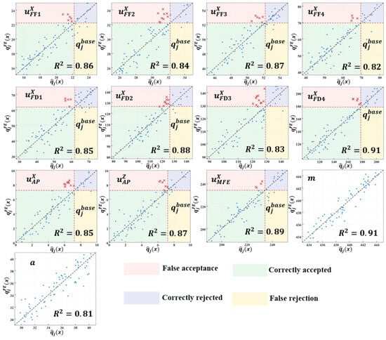
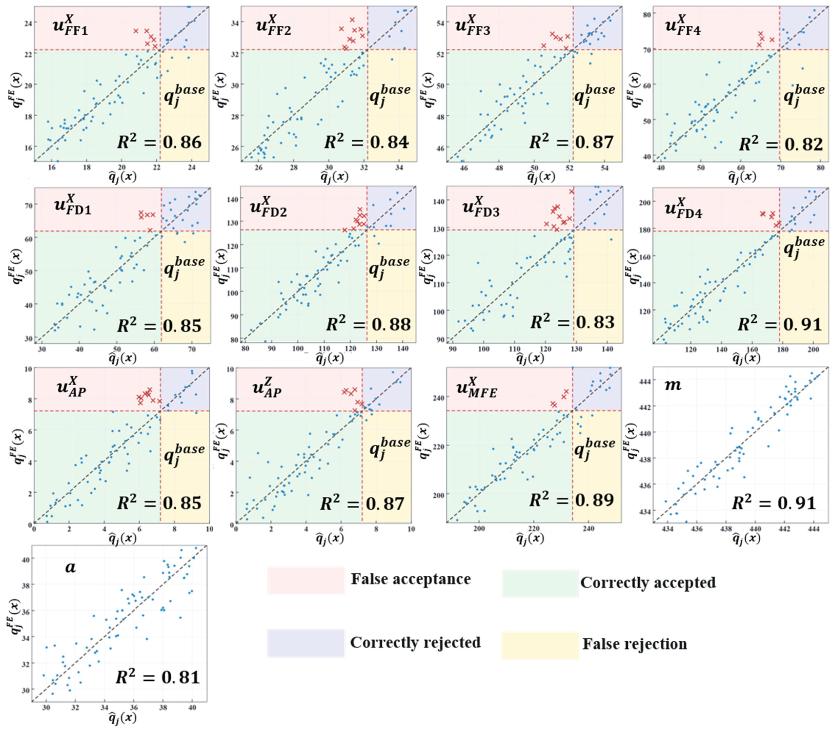
Figure 5 further compares surrogate predictions with FE results on the final test set. Body mass and vehicle acceleration were used only to evaluate the prediction accuracy of the optimization objectives and were not involved in baseline-referenced constraint decisions. The horizontal axis represents the surrogate-predicted risk value, and the vertical axis represents the FE risk value; the horizontal and vertical dashed lines correspond to the baseline-referenced boundary. The lower-left region indicates correct acceptance, where both the surrogate and FE results determine that the response is not degraded. The upper-right region indicates correct rejection. The lower-right region indicates false rejection, and the upper-left region indicates false acceptance, where the surrogate prediction satisfies the constraint, but the FE result shows that the response is actually worse than the baseline.

Figure 5. Prediction accuracy of the 13 output responses on the final test set and risk-boundary classification results for the 11 safety constraints.

Overall, most scatter points for the 13 output responses are distributed near the diagonal, indicating that RGEC-SM has high overall prediction accuracy. However, false-acceptance points still appear near the boundaries for some safety responses. Thus, high global R2 alone cannot guarantee reliable discrimination near constraint boundaries. For an optimization problem constrained by non-degradation relative to the initial design, nominal feasibility screening based only on the prediction mean may still retain candidates that actually violate safety constraints. This motivates the subsequent introduction of uncertainty calibration and conservative constraint decisions.

4.2. Model Ablation and FE Consistency of Variable-Group Relevance

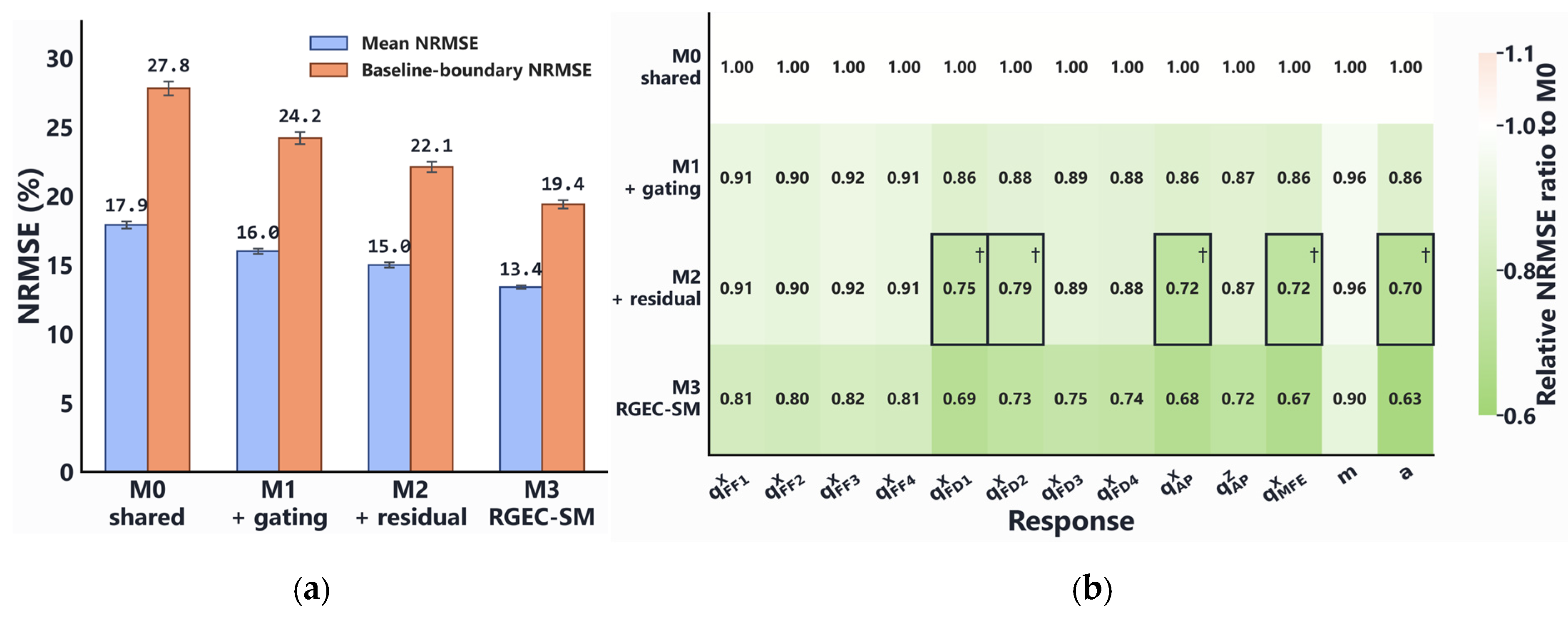
To isolate the contribution of response-dependent feature gating, M0 and M1 employed the same shared encoder, response-specific output heads, data partitions, and training settings, with gating introduced only in M1. As reported in Table 5, the mean test R² increased from 80.94% to 83.97%, while the mean NRMSE and Boundary-NRMSE decreased from 17.9% to 16.0% and from 27.8% to 24.2%, respectively. These correspond to relative error reductions of 10.6% and 12.9%. Both improvements were statistically significant across 10 matched-seed training repetitions (paired tests, p < 0.01). The reduction in Boundary-NRMSE further demonstrates improved prediction accuracy near the safety constraint thresholds, independently of the subsequent residual compensation and bootstrap ensembling.

Table 5. Ablation performance of RGEC-SM on the independent test set.

Model	Mean R2 (%)	R2 Range (%)	Mean NRMSE (%)	Boundary-NRMSE (%)	${\mathit{R}}_{{\mathit{u}}_{\mathit{FD}1}^{\mathit{x}}}^2$	${\mathit{R}}_{{\mathit{u}}_{\mathit{AP}}^{\mathit{x}}}^2$	${\mathit{R}}_{{\mathit{u}}_{\mathit{MFE}}^{\mathit{x}}}^2$	${\mathit{R}}_{\mathit{a}}^2$	Compensated Responses
M0: shared baseline	80.94	72.86~85.91	17.9	27.8	72.86	76.44	84.38	73.52	0/13
M1: M0 + gating	83.97	76.58~88.24	16.0	24.2	77.96	80.82	86.71	77.61	0/13
M2: M1 + conditional residual correction	85.24	76.58–90.10	15.0	22.1	77.96	83.45	88.60	80.96	5/13
M3: RGEC-SM	86.69	81.74~91.86	13.4	19.4	82.63	84.92	89.74	81.74	5/13

M2 activated residual compensation for only five of the 13 responses, reducing the independent-test mean NRMSE from 16.0% to 15.0% and Boundary-NRMSE from 24.2% to 22.1%, corresponding to relative reductions of 6.3% and 8.7%, respectively. The remaining eight responses, for which compensation was not enabled, retained the main predictions from M1 and therefore did not introduce new fitting disturbances through additional compensators. These results indicate that OOF-RBF compensation primarily corrects responses with stable local bias rather than uniformly modifying all outputs.

On the basis of M2, bootstrap ensembling increased the mean R2 to 86.69% and reduced the mean NRMSE and Boundary-NRMSE to 13.4% and 19.4%, respectively. Ensemble averaging weakened the prediction fluctuations caused by training-sample perturbations and local fitting bias in individual submodels, while also improving point-prediction accuracy near constraint boundaries. Whether the prediction standard deviation among bootstrap submodels can be used for conservative constraint construction is examined in Section 4.3.

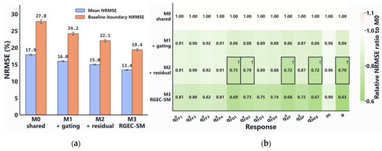
Figure 6 shows the effects of each module on the prediction error. Figure 6a shows that the mean NRMSE and Boundary-NRMSE decreased continuously from M0 to M3.

Figure 6. Ablation of response-specific gating, conditional OOF-RBF residual correction, and bootstrap ensembling. (a) Macro-averaged test NRMSE over 13 outputs and baseline-boundary NRMSE over 11 baseline-referenced constraint responses. Bars show mean values over 10 matched-seed independent training repetitions; error bars denote two-sided 95% confidence intervals across repetitions. (b) Test-set response-wise NRMSE ratios relative to M0. Black boxes and † identify the five responses receiving conditional OOF-RBF residual correction in M2; M3 uses the same correction configuration with a bootstrap ensemble.

Two-sided paired Wilcoxon signed-rank tests across the 10 independent training repetitions confirmed significant reductions in both mean NRMSE and Boundary-NRMSE between successive ablation models (all p < 0.01).

Figure 6b reports response-wise NRMSE ratios relative to M0:

$$r_{\mathcal{l},j}={\displaystyle \frac{{\mathrm{NRMSE}}_{\mathcal{l},j}}{{\mathrm{NRMSE}}_{\mathrm{M}0,j}}}$$

(18)

A value below 1 indicates that the prediction error of the model for the corresponding response is lower than that of M0. M1 reduced the error ratio below 1 for all 13 responses. In M2, changes occurred only for the five responses for which compensation was enabled. M3 further reduced the errors of the responses, with particularly clear improvements in accelerator-pedal intrusion, maximum front-end deformation, and vehicle acceleration.

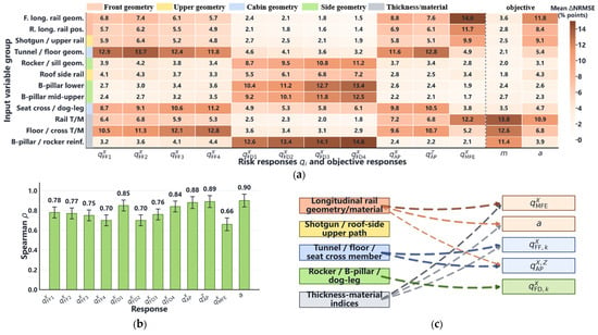
Based on the model accuracy analysis, a group-level conditional permutation method was further used to analyze the dependence of RGEC-SM on different variable groups. The geometric/positional variables and material-thickness variables were divided into 12 structural region groups. For a variable group and response, the relevance metric was defined as the mean increase in test error after repeated permutations:

$$I_{g,j}={\displaystyle \frac{1}{R}}{\displaystyle {\sum }_{r=1}^R}\left[{\mathrm{NRMSE}}_j\left({\tilde{\mathcal{D}}}_{\mathrm{test},g}^{\left(r\right)}\right)-{\mathrm{NRMSE}}_j\left({\mathcal{D}}_{\mathrm{test}}\right)\right],\mathit{R}=30$$

(19)

where $D_{\mathrm{test},g}^{\left(r\right)}$ denotes the test set obtained after the r-th conditional permutation of variable group g.

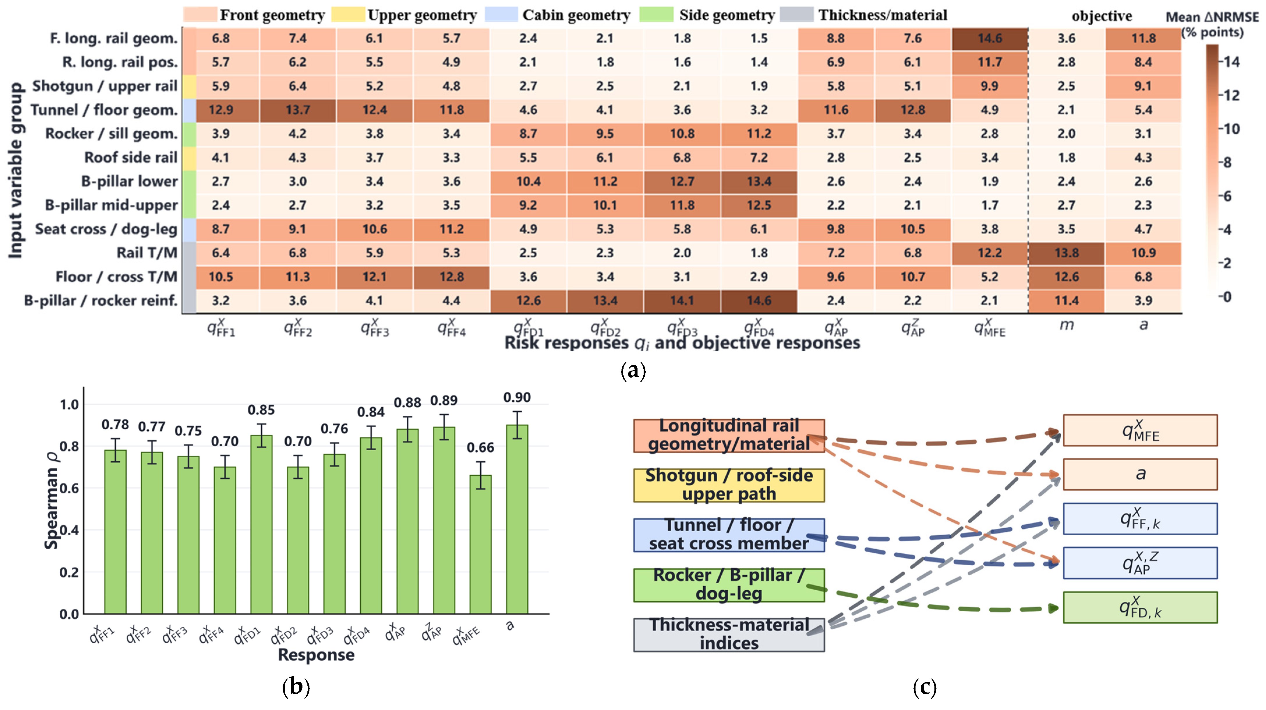
Figure 7a shows that the highly relevant variable groups differ markedly among responses. Front-floor risk is mainly associated with tunnel/floor geometry, floor/cross-member material-thickness variables, and the seat-cross/dog-leg region. Front-door risk is mainly associated with the B-pillar, rocker/sill, and their reinforcements. Accelerator-pedal risk is influenced by the tunnel/floor, seat-cross/dog-leg, and front-rail-related variable groups. Maximum front-end deformation risk and vehicle acceleration are mainly associated with front-rail geometry, shotgun/upper-rail variables, and rail material-thickness variables. These patterns are consistent with the basic characteristics of front-compartment crushing, floor load transfer, side-frame and door-frame deformation, and deceleration-pulse control. Body mass in Figure 7a is retained only as an auxiliary output to reflect the direct relationship between material-thickness variable groups and mass prediction. Because mass is not a crash load-transfer response and can be calculated directly from the parametric model, it is not included in the subsequent consistency evaluation of FE sensitivity rankings.

Figure 7. Group-wise conditional permutation relevance of RGEC-SM and consistency with FE local sensitivity trends. (a) Mean increase in test NRMSE after R = 30 conditional group permutations. The 11 safety-related outputs are represented as baseline-referenced risk responses; mass m and vehicle acceleration a are retained as objective responses. (b) Spearman rank correlation between surrogate group relevance and separately performed FE local sensitivity for the 11 baseline-referenced risk responses and vehicle acceleration; mass is excluded. (c) Aggregated relevance map derived from the top three group-response relevance links in panel (a). Dashed arrows denote model relevance associations rather than unique physical load-transfer paths or causal effects; line thickness represents averaged group-wise permutation relevance within each response category.

To examine the consistency between surrogate-based variable-group ranking and local FE response trends, 12 feasible reference designs were selected outside the training, validation, calibration, and test samples for group-level FE perturbation analysis. The local FE sensitivity of each variable group to each response was defined as follows:

$$S_{g,j}^{\mathrm{FE}}={\mathrm{median}}_{t,v,p}\left[{\displaystyle \frac{\left|r_j^{\mathrm{FE}}\left({\mathbf{x}}_{t,v,p}\right)-r_j^{\mathrm{FE}}\left({\mathbf{x}}_t\right)\right|}{d_{t,v,p}{R}_{j,\mathit{train}}}}\right]$$

(20)

where x_t denotes the t-th reference design, x_t,v,p denotes the corresponding perturbed design for variable v within group g under perturbation state p, and d_t,v,p is the normalized input step. Safety responses use the risk quantity, while the objective responses retain only vehicle acceleration. The relevance metric and FE sensitivity for each response were then ranked separately, and Spearman rank correlation coefficients were calculated.

In Figure 7b, excluding mass, the Spearman correlation coefficients between surrogate variable-group relevance and FE local-sensitivity rankings range from 0.66 to 0.90. The floor-pedal-related responses and vehicle acceleration show high ranking consistency, with the highest coefficient reaching 0.90. The correlation coefficient for maximum front-end deformation risk is 0.66, indicating that this response is jointly affected by the front-compartment crushing mode, material-thickness configuration, and geometric position; a single variable-group ranking cannot fully describe its deformation mechanism.

Figure 7c summarizes the three variable groups with the highest relevance in each response category. The dashed connections indicate only variable group-response associations identified by the surrogate model and should not be interpreted as unique physical load paths or strict causal relationships. During subsequent optimization, if a baseline-referenced risk increases, local FE re-simulation and structural adjustment can first focus on the highly relevant variable groups. The final control direction should still be determined together with deformation mode, energy absorption, and load transfer behavior.

4.3. Uncertainty Calibration and Conservative Feasibility Verification

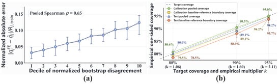
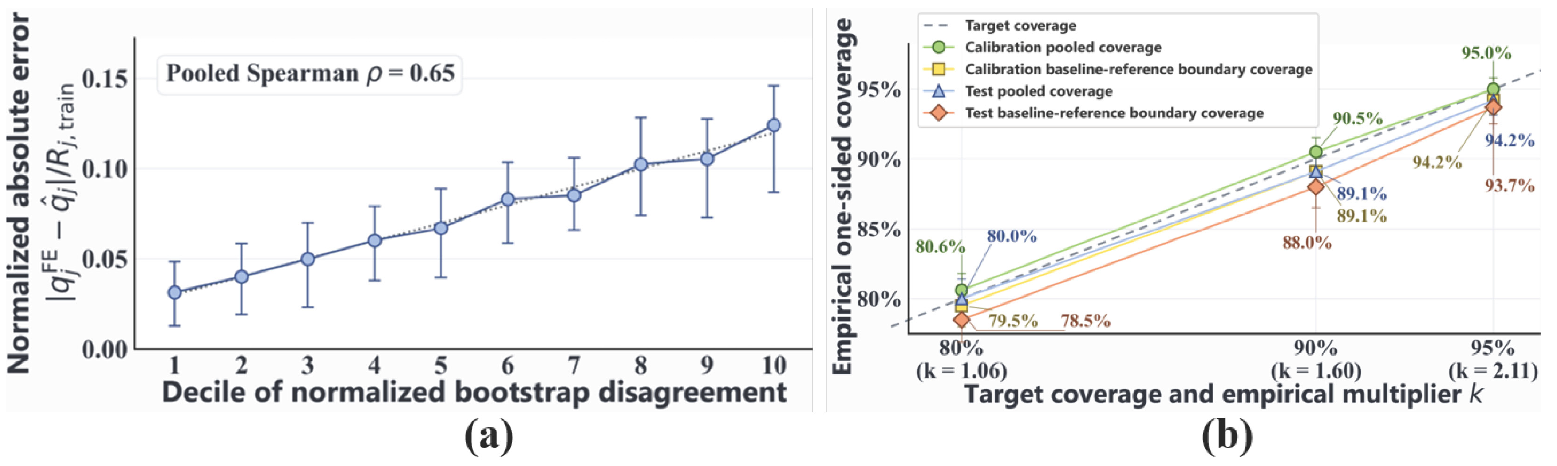
This section examines whether the bootstrap ensemble standard deviation can be calibrated for baseline-referenced constraint screening. For the 11 safety-related responses, the risk multiplier was determined on an independent calibration set using a 90% pooled one-sided marginal coverage target. Table 6 reports the empirical coverage of the unscaled and calibrated upper bounds.

Table 6. Empirical one-sided coverage of unscaled and calibrated upper bounds for baseline-referenced constraint responses.

Dataset	Evaluation Subset	Sample–Constraint Pairs	Unscaled Upper Bound, k = 1.0	Calibrated Upper Bound, k = 1.6
Dcal	Pooled responses	660	480/660 = 72.7%	597/660 = 90.5%
Dcal	Baseline-boundary subset	156	116/156 = 74.4%	139/156 = 89.1%
Dtest	Pooled responses	660	473/660 = 71.7%	588/660 = 89.1%
Dtest	Baseline-boundary subset	158	115/158 = 72.8%	139/158 = 88.0%

Before calibration, the upper-bound coverage corresponding to ensemble disagreement was only 71.7–74.4%, and therefore could not be used directly as a conservative prediction bound for safety constraints. After introducing the risk multiplier, the pooled coverage reached 90.5% on the calibration set and 89.1% on the final test set; the corresponding boundary-subset coverages were 89.1% and 88.0%. Thus, calibration improved the reliability of the upper prediction bound overall, but it still did not provide a strict 90% coverage guarantee for every local response or boundary region. The empirical joint coverage across all 11 safety responses was 41/60 (68.3%) on the independent test set, compared with the pooled marginal coverage of 89.1%. The lower joint coverage reflects the cumulative effect of prediction errors across multiple safety responses. The results indicate that simultaneous coverage of all 11 responses is more demanding than pooled marginal coverage.

Figure 8a further examines the ability of ensemble disagreement to rank prediction errors. After sample-response pairs in the test set were divided into 10 quantile groups according to normalized prediction standard deviation, the normalized absolute error generally increased with uncertainty level. Response-wise Spearman rank correlation coefficients ranged from 0.42 to 0.73, with a median of approximately 0.59. Bootstrap disagreement can therefore identify high-error-risk regions, but cannot accurately estimate pointwise error magnitude. Figure 8b compares calibration results under 80%, 90%, and 95% target coverage levels. This study uses only the multiplier corresponding to the 90% target to construct conservative constraints; the other coverage levels are shown only to illustrate the influence of risk preference on calibration results.

Figure 8. Uncertainty ranking and empirical one-sided calibration for baseline-referenced constraint responses: (a) relationship between normalized bootstrap disagreement and normalized absolute error on the independent test set; (b) pooled and baseline-boundary coverage on calibration and test sets under different target coverage levels.

To evaluate conservative constraint screening, the candidate list was frozen after optimization, and 48 unique designs were selected after duplicate removal using constraint-status stratification, boundary proximity, and objective-space diversity criteria. The selection included 29 conservatively accepted, eight nominally accepted but conservatively rejected, and 11 nominally rejected candidates, while accounting for their proximity to the safety constraint boundaries and distribution in the normalized mass–acceleration objective space. The same 48 designs were subsequently evaluated under both nominal and conservative decision rules using FE results. To unify nominal decisions, conservative decisions, and FE re-simulation results, the maximum normalized violation of a candidate was defined as follows:

$$G^{\mathrm{nom}}\left(\mathbf{x}\right)=\underset{j\in \mathcal{C}}{\max }{\displaystyle \frac{{\widehat{q}}_j\left(\mathbf{x}\right)-q_j^{\mathrm{base}}}{R_{j,\mathit{train}}}}$$

(21)

$$G^{\mathrm{cons}}\left(\mathbf{x}\right)=\underset{j\in \mathcal{C}}{\max }{\displaystyle \frac{{\widehat{q}}_j\left(\mathbf{x}\right)+k{\sigma }_j\left(\mathbf{x}\right)-q_j^{\mathrm{base}}}{R_{j,\mathit{train}}}}$$

(22)

$$G^{\mathrm{FE}}\left(\mathbf{x}\right)=\underset{j\in \mathcal{C}}{\max }{\displaystyle \frac{q_j^{\mathrm{FE}}\left(\mathbf{x}\right)-q_j^{\mathrm{base}}}{R_{j,\mathit{train}}}}$$

(23)

where the response range in the training set is used for normalization. When the nominal, conservative, or FE violation measure is no greater than zero, the candidate satisfies all baseline-referenced non-degradation constraints under nominal prediction, conservative prediction, or FE re-simulation, respectively.

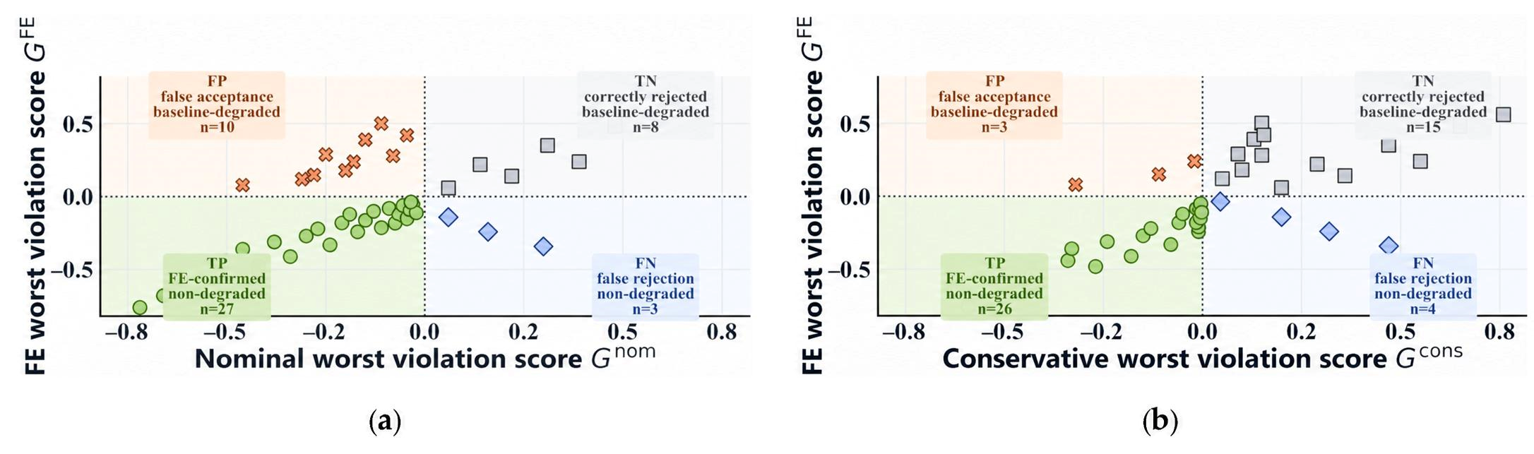
Table 7 reports the candidate-level FE audit results. The nominal decision accepted 37 candidates, of which 27 were confirmed by FE to be no worse than the baseline design, giving an acceptance precision of 73.0% and a false-acceptance rate of 27.0%. With the conservative decision, the number of accepted candidates decreased to 29, of which 26 were confirmed by FE to be no worse than the baseline. Acceptance precision increased to 89.7%, and the false-acceptance rate decreased to 10.3%. The conservative decision changed the classification of only eight boundary-uncertain candidates. Seven candidates that were actually worse than the baseline design were correctly rejected, while one non-degraded candidate was additionally rejected. Conservative screening therefore substantially reduced false-acceptance risk at the cost of losing a small number of feasible candidates. Because the 48 designs were deliberately selected to cover different constraint states and objective trade-offs, the reported error rates characterize screening performance within the audited candidate set rather than providing statistical estimates for the entire search population. Together with the independent-test Boundary-NRMSE of 19.4% and the calibrated near-boundary coverage of 88.0%, the candidate-level FE audit provides empirical evidence of the prediction and constraint-screening performance achieved with the 600-sample dataset, despite the limited sampling density of the high-dimensional design space.

Table 7. Candidate-level FE audit of nominal and conservative baseline-referenced feasibility decisions.

Decision Rule	Accepted Candidates	TP	FP	Rejected Candidates	FN	TN	Acceptance Precision	False-Acceptance Rate	FE Non-Degradation Retention	Specificity
Nominal decision	37	27	10	11	3	8	73.0%	27.0%	90.0%	44.4%
Conservative decision, k = 1.6	29	26	3	19	4	15	89.7%	10.3%	86.7%	83.3%

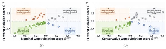
Figure 9 visualizes the nominal and conservative classification results using maximum normalized violation. After conservative decisions were implemented, the number of false-accepted candidates decreased from 10 to 3, and the number of true-rejected candidates increased from 8 to 15, consistent with the statistics in Table 7.

Figure 9. Finite-element audit of nominal and conservative baseline-referenced decisions for optimization candidates: (a) nominal decision; (b) conservative decision.

4.4. Multi-Run Search Performance and Conservative Baseline-Referenced Feasibility of UC-SB-NSGA-II

After uncertainty calibration and candidate FE auditing, NSGA-II and UC-SB-NSGA-II were further compared under a fixed surrogate-evaluation budget. Final-generation hypervolume and spacing were calculated only on the non-dominated solution set that satisfied conservative baseline-referenced feasibility. The objective-normalization range and reference point were fixed in advance. A smaller spacing value indicates a more uniform distribution in the objective space. Runtime includes only surrogate prediction, constraint evaluation, population sorting, and evolutionary operations, excluding surrogate-model training, risk calibration, TOPSIS ranking, and FE re-simulation.

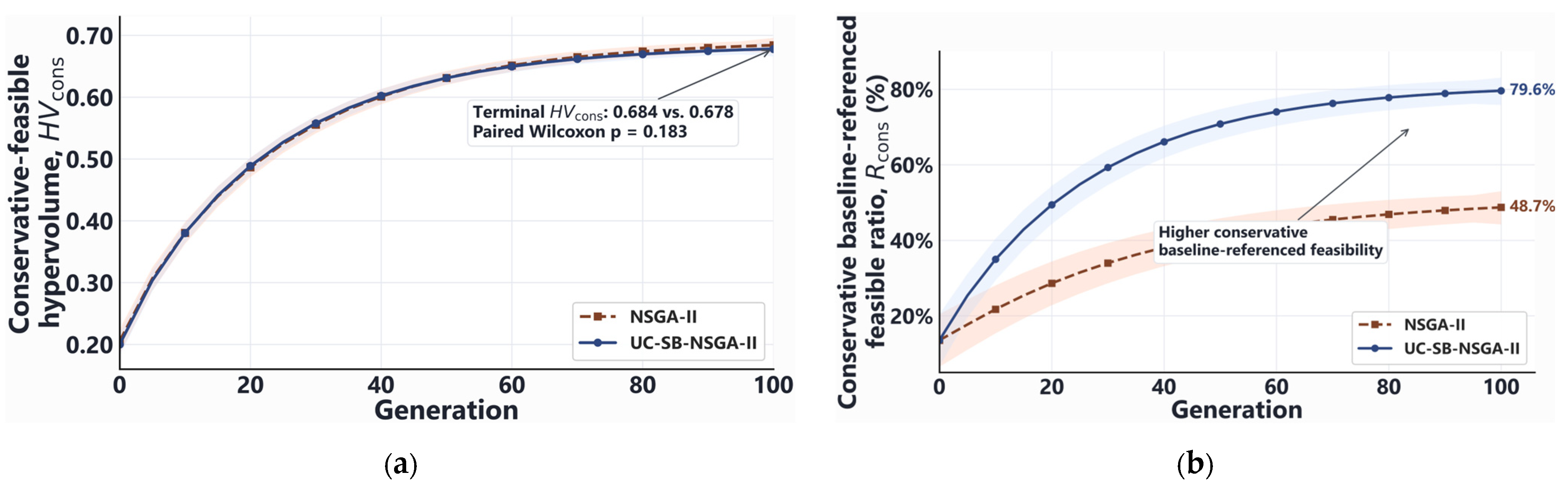
Table 8 reports the statistics from 20 paired runs. The final-generation hypervolume medians of NSGA-II and UC-SB-NSGA-II were 0.684 and 0.678, respectively, with similar interquartile ranges. This indicates that, under the present fixed budget and reference-point settings, introducing conservative constraint dominance did not cause an obvious loss of conservative-feasible objective space.

Table 8. Multi-run surrogate-search performance of NSGA-II and UC-SB-NSGA-II under a fixed optimization budget.

Algorithm	HVcons, Median [IQR]	Spacingcons, Median [IQR]	Rcons, Median [IQR]	Runtime, Median [IQR] (Min)
NSGA-II	0.684 [0.671, 0.696]	0.086 [0.079, 0.096]	48.7 [44.2, 53.0]%	11.2 [10.95, 11.47]
UC-SB-NSGA-II, k = 1.6	0.678 [0.666, 0.690]	0.079 [0.072, 0.087]	79.6 [75.8, 83.1]%	11.58 [11.31, 11.85]

The final-generation conservative baseline-referenced feasible ratio of UC-SB-NSGA-II increased from 48.7% to 79.6%, indicating that its environmental selection process preferentially retained candidates with lower combined risk from prediction mean and uncertainty. The median spacing decreased from 0.086 to 0.079, indicating that the conservatively feasible non-dominated solutions did not become markedly clustered. The median runtimes of the two algorithms were 11.20 min and 11.58 min; the additional cost introduced by conservative constraint handling was approximately 0.38 min, or about 3.4%. This increase mainly resulted from conservative violation calculation and environment selection based on conservative constraints.

Table 9. reports the paired Wilcoxon test, Holm-adjusted results, and rank-biserial effect sizes. After multiple-comparison correction, the improvement in conservative feasibility remained significant, while differences in hypervolume and spacing did not reach the 5% significance level. Thus, the advantage of UC-SB-NSGA-II is mainly reflected in changing the conservative-risk composition of the population, rather than outperforming NSGA-II in every search-quality indicator.

Table 9. Paired statistical comparison between UC-SB-NSGA-II and NSGA-II.

Metric	Wilcoxon Wmin	Raw p	Holm-Adjusted p	Rank-Biserial Effect Size
HVcons	69	0.183	0.183	−0.3
Spacingcons	50	0.042	0.082	0.46
Rcons	0	<0.001	<0.003	0.88

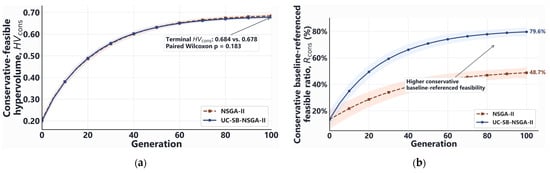
Figure 10 shows the median and interquartile-range evolution of the two algorithms. In Figure 10a, the hypervolume curves of the two algorithms are generally close, indicating that conservative constraint dominance did not significantly compress the conservative-feasible objective space. In Figure 10b, both algorithms start from the same feasible ratio at generation 0 and then gradually diverge. NSGA-II can maintain a certain proportion of conservatively feasible candidates, but its population still contains many individuals satisfying only nominal constraints. UC-SB-NSGA-II continuously increases the proportion of candidates satisfying all conservative constraints. Its role is therefore not to expand the nominal Pareto front, but to increase the proportion of conservatively baseline-referenced feasible candidates under a fixed surrogate-evaluation budget.

Figure 10. Multi-run surrogate-search performance of UC-SB-NSGA-II and NSGA-II under a fixed optimization budget: (a) conservative-feasible hypervolume shown as median with IQR band; (b) conservative baseline-referenced feasible ratio shown as median with IQR band.

4.5. FE-Confirmed Reliable Pareto Trade-Offs and Final Design Verification

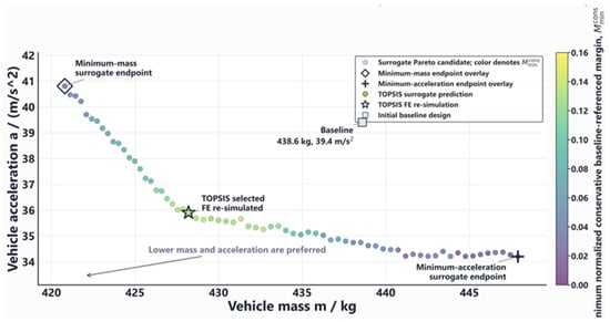
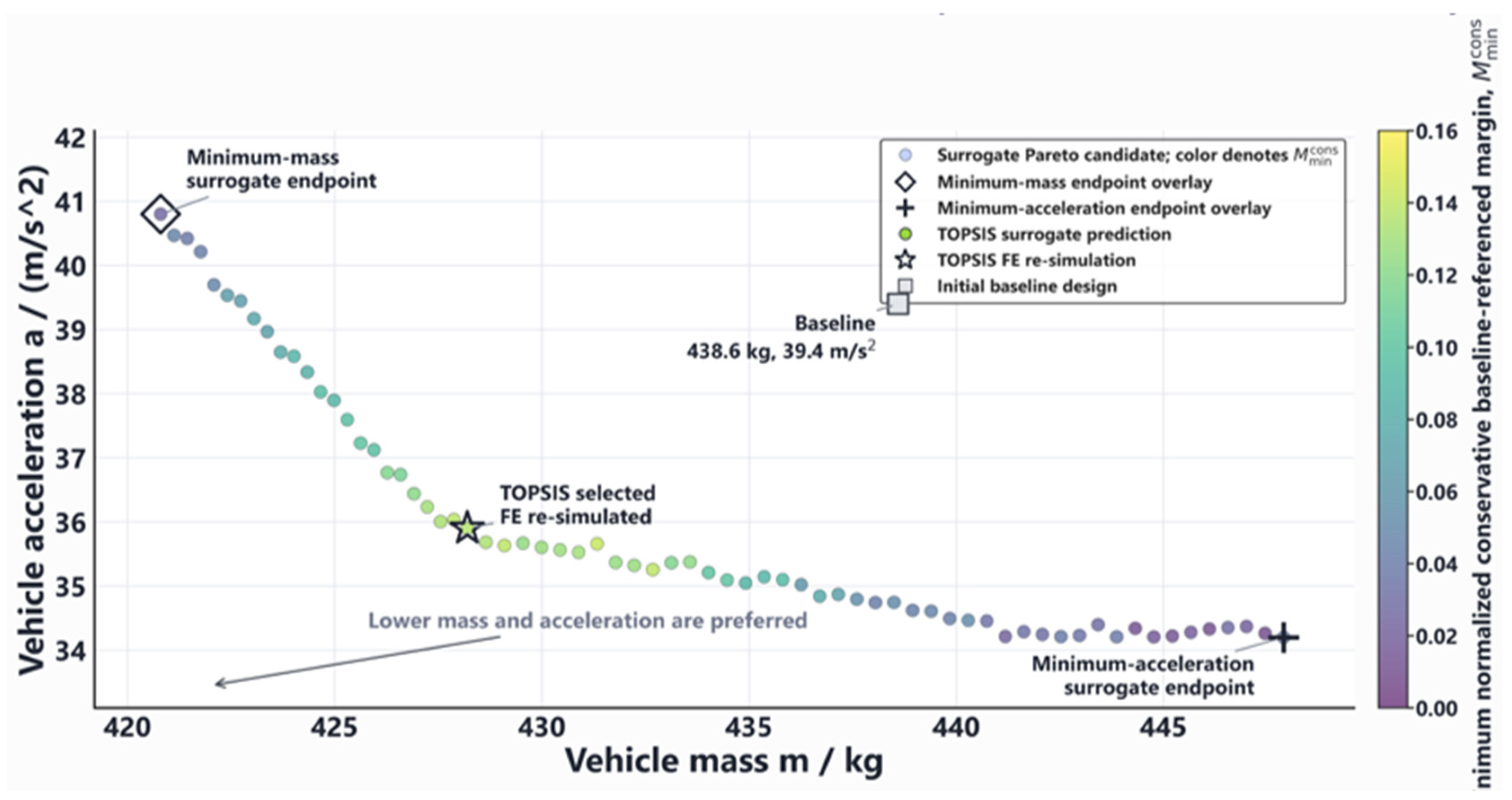
To determine the final recommended design, the UC-SB-NSGA-II run whose final generation was closest to the median of the 20 paired runs was selected as the representative run. After duplicate candidates were removed from its final conservatively baseline-referenced feasible non-dominated set, a Pareto set was obtained. TOPSIS was applied only within this set, using body mass, vehicle acceleration, and the minimum normalized conservative baseline-referenced margin defined in Section 3.2.4 as evaluation indicators. Figure 11 shows the objective distribution of conservatively baseline-referenced feasible Pareto candidates in the representative run. The lightest candidate and the lowest-acceleration candidate are located at opposite ends of the Pareto front. The TOPSIS-recommended design lies between them and provides a compromise among mass, vehicle acceleration, and conservative baseline-referenced margin.

Figure 11. Surrogate-screened, conservatively baseline-referenced feasible Pareto candidates from the representative UC-SB-NSGA-II run and the TOPSIS-selected candidate re-simulated by FE.

The results in Table 10 are surrogate predictions. The predicted mass of the minimum-mass candidate decreased by 4.06%, but its vehicle acceleration increased by 3.55%. The predicted vehicle acceleration of the minimum-acceleration candidate decreased by 13.20%, but its mass increased by 2.12%. The TOPSIS-recommended candidate reduced the predicted mass and vehicle acceleration by 2.37% and 8.88%, respectively, and retained a larger conservative baseline-referenced margin than the two endpoint candidates. This design does not rely only on approaching a single constraint boundary to obtain objective improvement; instead, it retains a larger conservative baseline-referenced margin at the surrogate level.

Table 10. Surrogate-level representative conservatively baseline-referenced feasible Pareto candidates.

Scheme	m (kg), Surrogate	Change	a (m/s2), Surrogate	Change	${\mathit{M}}_{\mathit{min}}^{\mathit{cons}}$	TOPSIS Closeness	TOPSIS Rank
Baseline	438.6	-	39.4	-	-	-	-
Minimum mass	420.8	−4.06%	40.8	+3.55%	0.026	0.519	7
Minimum acceleration	447.9	+2.12%	34.2	−13.20%	0.043	0.638	4
TOPSIS-assisted final candidate	428.2	−2.37%	35.9	−8.88%	0.136	0.783	1

To examine surrogate-prediction consistency for the recommended design and to confirm whether its 11 safety-related responses satisfied the requirement of no degradation relative to the initial baseline design, the TOPSIS candidate was re-simulated using FE analysis. Table 11 shows that all 11 safety-related responses of the TOPSIS-recommended candidate had positive FE baseline-referenced margins, defined as the differences between the baseline risk thresholds and the corresponding FE risk values. The minimum margin was 1.9 mm, indicating that this response was the most adverse safety constraint in the final design, but it was still not worse than the initial baseline. The absolute prediction errors of the safety responses ranged from 3.96% to 9.23%. All margins in Table 11 are greater than 0, demonstrating that the candidate satisfies the 11 baseline-referenced non-degradation constraints within the present FE model system.

Table 11. FE audit of baseline-referenced constraint responses for the TOPSIS-selected candidate.

Response	${\mathit{q}}_{\mathit{j}}^{\mathit{base}}$	${\widehat{\mathit{q}}}_{\mathit{j}}$	${\widehat{\mathit{q}}}_{\mathit{j}}+\mathit{k}{\mathit{\sigma }}_{\mathit{j}}$	${\mathit{q}}_{\mathit{j}}^{\mathit{FE}}$	${\mathit{M}}_{\mathit{j}}^{\mathit{FE}}$	Absolute Prediction Error
$u_{\mathit{FF}1}^X$	116.8	102.9	110.6	112.4	4.4	9.23%
$u_{\mathit{FF}2}^X$	112.7	107.3	110.1	101.3	11.3	5.50%
$u_{\mathit{FF}3}^X$	123.5	110.7	118.7	118.4	5.1	6.96%
$u_{\mathit{FF}4}^X$	127.4	112.4	121.4	121.8	5.6	8.36%
$u_{\mathit{FD}1}^X$	58.2	55.6	57.2	51.4	6.8	7.55%
$u_{\mathit{FD}2}^X$	65.4	59.0	62.2	62.7	2.6	6.44%
$u_{\mathit{FD}3}^X$	65.0	61.9	63.2	56.9	8.1	8.08%
$u_{\mathit{FD}4}^X$	67.6	63.2	66.9	65.7	1.9	3.96%
$u_{\mathit{AP}}^X$	100.5	95.6	98.2	88.2	12.3	7.74%
$u_{\mathit{AP}}^Z$	112.0	103.6	108.9	109.6	2.4	5.79%
$u_{\mathit{MFE}}^X$	241.1	231.3	236.3	218.9	22.1	5.36%

Table 12 shows that the surrogate-predicted mass reduction of 2.37% increased to 4.15% after FE re-simulation, while the predicted vehicle-acceleration reduction of 8.88% retained a 6.35% improvement after re-simulation.

Table 12. FE re-simulation results for optimization objectives of the TOPSIS-selected candidate.

Objective	Baseline Value	Surrogate Prediction	FE Re-Simulation	Absolute Surrogate–FE Error	FE Change from Baseline
Body mass (kg)	438.6	428.2	420.4	1.85%	−4.15%
Vehicle acceleration (m/s2)	39.4	35.9	36.9	2.79%	−6.35%

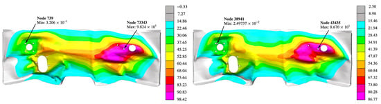
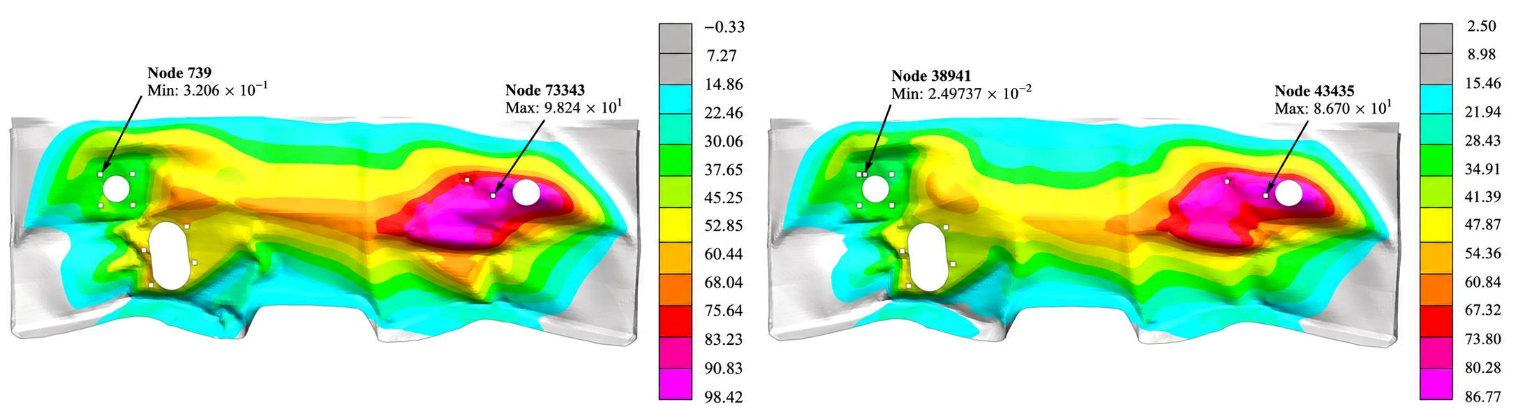
Figure 12 shows that the peak longitudinal displacement in the plotted field decreases from approximately 98.42 mm in the baseline design to 86.68 mm in the TOPSIS-recommended design, a reduction of about 11.9%. At the defined $u_{\mathit{FD}2}^X$ response point, the FE result also decreases from 65.4 mm to 62.7 mm. The hotspot remains in the same local region but has a lower magnitude, indicating that the optimized design mitigates rather than transfers the dominant deformation.

Figure 12. FE longitudinal-displacement contours for the front-door response ($u_{\mathit{FD}2}^X$): baseline design (left) and TOPSIS-recommended design (right).

The FE audit of 48 modified candidates (Table 7), together with the re-simulation of the TOPSIS-selected design (Table 11 and Table 12 and Figure 12), provides numerical verification of the surrogate predictions for modified structural configurations. Among the 29 conservatively accepted candidates in the FE audit, 26 satisfied all 11 safety constraints, corresponding to an acceptance precision of 89.7%. This provides evidence of conservative screening performance across multiple designs, although the FE audit does not establish the feasibility of every solution in the surrogate-screened Pareto set. These results assess the consistency between surrogate predictions and full-vehicle FE responses, while experimental validation of the modified configurations remains outside the scope of the present study.

5. Conclusions

This study developed a surrogate-assisted optimization workflow combining RGEC-SM and UC-SB-NSGA-II for the 68-dimensional mixed-variable optimization problem of electric vehicle frontal crashworthiness. The main conclusions are as follows:

• RGEC-SM effectively predicted body mass, vehicle acceleration, and 11 safety responses. On the independent test set, R2 values for the 13 responses ranged from 81.74% to 91.86%, the mean NRMSE was 13.4%, and the Boundary-NRMSE near safety constraint boundaries was 19.4%. Response gating, conditional residual compensation, and bootstrap ensembling all contributed to improved prediction accuracy.
• After independent calibration, bootstrap prediction disagreement could be used to construct conservative constraints. With the selected risk multiplier, the false-acceptance rate in the candidate audit decreased from 27% to 10.3%, and acceptance precision increased from 73.0% to 89.7%. UC-SB-NSGA-II increased the final-generation conservative feasible ratio from 48.7% to 79.6% while maintaining a broadly stable conservative-feasible hypervolume.
• FE re-simulation of the TOPSIS-recommended design confirmed that all 11 safety responses were no worse than those of the initial baseline design. Body mass decreased by 4.15%, and vehicle acceleration decreased by 6.35%. The proposed method can coordinate lightweighting, acceleration control, and safety constraints under a limited simulation budget while reducing feasibility misclassification risk in surrogate-based optimization.

However, the uncertainty considered in this study characterizes only surrogate-model prediction disagreement. It does not include material variability, manufacturing error, connection failure, or FE model-form uncertainty. Future work could combine active sampling, connection failure modeling, and multi-source uncertainty propagation to further improve the engineering reliability of the optimization results. Further experimental or component-level validation of representative modified configurations is needed to assess the transferability of the baseline FE model validation.

References

- Fang, H.; Rais-Rohani, M.; Liu, Z.; Horstemeyer, M.F. A comparative study of metamodeling methods for multiobjective crashworthiness optimization. Comput. Struct. 2005, 83, 2121–2136. [Google Scholar] [CrossRef] [Scilit]
- Fang, J.; Sun, G.; Qiu, N.; Kim, N.H.; Li, Q. On design optimization for structural crashworthiness and its state of the art. Struct. Multidiscip. Optim. 2017, 55, 1091–1119. [Google Scholar] [CrossRef] [Scilit]
- Marklund, P.-O.; Nilsson, L. Optimization of a car body component subjected to side impact. Struct. Multidiscip. Optim. 2001, 21, 383–392. [Google Scholar] [CrossRef] [Scilit]
- Kim, H.M.; Michelena, N.F.; Papalambros, P.Y.; Jiang, T. Development of simplified models for design and optimization of automotive structures for crashworthiness. Struct. Multidiscip. Optim. 2001, 22, 307–321. [Google Scholar] [CrossRef] [Scilit]
- Redhe, M.; Nilsson, L. Using the response surface methodology and the D-optimality criterion in crashworthiness related problems. Struct. Multidiscip. Optim. 2002, 24, 185–194. [Google Scholar] [CrossRef] [Scilit]
- Avalle, M.; Belingardi, G.; Montanini, R. Design optimization by response surface methodology: Application to crashworthiness design of vehicle structures. Struct. Multidiscip. Optim. 2002, 24, 325–332. [Google Scholar] [CrossRef] [Scilit]
- Kirkpatrick, S.W.; MacNeill, R.A.; Kirkpatrick, S.W. Development and validation of high fidelity vehicle crash simulation models. Int. J. Crashworthiness 1999, 4, 395–410. [Google Scholar] [CrossRef] [Scilit]
- Zaouk, A.K.; Bedewi, N.E.; Kan, C.-D.; Marzougui, D. Development of a detailed vehicle finite element model. Part I: Methodology. Int. J. Crashworthiness 2000, 5, 25–36. [Google Scholar] [CrossRef] [Scilit]
- Zaouk, A.K.; Bedewi, N.E.; Kan, C.-D.; Marzougui, D. Development of a detailed vehicle finite element model. Part II: Material characterization and component testing. Int. J. Crashworthiness 2000, 5, 37–50. [Google Scholar] [CrossRef] [Scilit]
- Kan, C.-D.; Marzougui, D.; Bedewi, N.E. Crashworthiness evaluation using integrated vehicle and occupant finite element models. Int. J. Crashworthiness 2001, 6, 387–398. [Google Scholar] [CrossRef] [Scilit]
- Shaikh, S.A.; Cherukuri, H.; Balusu, K.; Devanathan, R.; Soulami, A. Probabilistic surrogate model for accelerating the design of electric vehicle battery enclosures for crash performance. arXiv 2024, arXiv:2408.03450. [Google Scholar]
- McKay, M.D.; Beckman, R.J.; Conover, W.J. A comparison of three methods for selecting values of input variables in the analysis of output from a computer code. Technometrics 1979, 21, 239–245. [Google Scholar] [CrossRef] [Scilit]
- Sacks, J.; Welch, W.J.; Mitchell, T.J.; Wynn, H.P. Design and analysis of computer experiments. Stat. Sci. 1989, 4, 409–423. [Google Scholar] [CrossRef] [Scilit]
- Alexandrov, N.M.; Dennis, J.E.; Lewis, R.M.; Torczon, V. A trust region framework for managing the use of approximation models in optimization. Struct. Optim. 1998, 15, 16–23. [Google Scholar] [CrossRef] [Scilit]
- Booker, A.J.; Dennis, J.E.; Frank, P.D.; Serafini, D.B.; Torczon, V.; Trosset, M.W. A rigorous framework for optimization of expensive functions by surrogates. Struct. Optim. 1999, 17, 1–13. [Google Scholar] [CrossRef]
- Queipo, N.V.; Haftka, R.T.; Shyy, W.; Goel, T.; Vaidyanathan, R.; Tucker, P.K. Surrogate-based analysis and optimization. Prog. Aerosp. Sci. 2005, 41, 1–28. [Google Scholar] [CrossRef] [Scilit]
- Simpson, T.W.; Peplinski, J.D.; Koch, P.N.; Allen, J.K. Metamodels for computer-based engineering design: Survey and recommendations. Eng. Comput. 2001, 17, 129–150. [Google Scholar] [CrossRef] [Scilit]
- Forrester, A.I.J.; Sobester, A.; Keane, A.J. Engineering Design via Surrogate Modelling: A Practical Guide; Wiley: Chichester, UK, 2008. [Google Scholar]
- Jones, D.R.; Schonlau, M.; Welch, W.J. Efficient global optimization of expensive black-box functions. J. Glob. Optim. 1998, 13, 455–492. [Google Scholar] [CrossRef] [Scilit]
- Lophaven, S.N.; Nielsen, H.B.; Sondergaard, J. DACE: A MATLAB Kriging Toolbox; Technical Report IMM-TR-2002-12; Technical University of Denmark: Lyngby, Denmark, 2002. [Google Scholar]
- Buhmann, M.D. Radial Basis Functions: Theory and Implementations; Cambridge University Press: Cambridge, UK, 2003. [Google Scholar]
- Jin, Y. Surrogate-assisted evolutionary computation: Recent advances and future challenges. Swarm Evol. Comput. 2011, 1, 61–70. [Google Scholar] [CrossRef] [Scilit]
- Wang, G.G.; Shan, S. Review of metamodeling techniques in support of engineering design optimization. J. Mech. Des. 2007, 129, 370–380. [Google Scholar] [CrossRef] [Scilit]
- Broomhead, D.S.; Lowe, D. Radial basis functions, multi-variable functional interpolation and adaptive network. Complex Syst. 1988, 2, 321–355. [Google Scholar]
- Cortes, C.; Vapnik, V. Support-vector networks. Mach. Learn. 1995, 20, 273–297. [Google Scholar] [CrossRef] [Scilit]
- Smola, A.J.; Scholkopf, B. A tutorial on support vector regression. Stat. Comput. 2004, 14, 199–222. [Google Scholar] [CrossRef] [Scilit]
- Rumelhart, D.E.; Hinton, G.E.; Williams, R.J. Learning representations by back-propagating errors. Nature 1986, 323, 533–536. [Google Scholar] [CrossRef] [Scilit]
- Friedman, J.H. Multivariate adaptive regression splines. Ann. Stat. 1991, 19, 1–67. [Google Scholar] [CrossRef] [Scilit]
- Huber, P.J. Robust estimation of a location parameter. Ann. Math. Stat. 1964, 35, 73–101. [Google Scholar] [CrossRef] [Scilit]
- MacQueen, J. Some methods for classification and analysis of multivariate observations. In Proceedings of the Fifth Berkeley Symposium on Mathematical Statistics and Probability; University of California Press: Berkeley, CA, USA, 1967; Volume 1, pp. 281–297. [Google Scholar]
- Stone, M. Cross-validatory choice and assessment of statistical predictions. J. R. Stat. Soc. Ser. B 1974, 36, 111–133. [Google Scholar] [CrossRef] [Scilit]
- Kohavi, R. A study of cross-validation and bootstrap for accuracy estimation and model selection. In Proceedings of the 14th International Joint Conference on Artificial Intelligence; Morgan Kaufmann: San Francisco, CA, USA, 1995; pp. 1137–1143. [Google Scholar]
- Efron, B. Bootstrap methods: Another look at the jackknife. Ann. Stat. 1979, 7, 1–26. [Google Scholar] [CrossRef] [Scilit]
- Breiman, L. Bagging predictors. Mach. Learn. 1996, 24, 123–140. [Google Scholar] [CrossRef] [Scilit]
- Lakshminarayanan, B.; Pritzel, A.; Blundell, C. Simple and scalable predictive uncertainty estimation using deep ensembles. In Advances in Neural Information Processing Systems; Curran Associates: Red Hook, NY, USA, 2017; Volume 30. [Google Scholar]
- Guo, C.; Pleiss, G.; Sun, Y.; Weinberger, K.Q. On calibration of modern neural networks. In Proceedings of the 34th International Conference on Machine Learning; PMLR: Sydney, Australia, 2017; Volume 70, pp. 1321–1330. [Google Scholar]
- Kuleshov, V.; Fenner, N.; Ermon, S. Accurate uncertainties for deep learning using calibrated regression. In Proceedings of the 35th International Conference on Machine Learning; PMLR: Stockholm, Sweden, 2018; Volume 80, pp. 2796–2804. [Google Scholar]
- Lei, J.; G’Sell, M.; Rinaldo, A.; Tibshirani, R.J.; Wasserman, L. Distribution-free predictive inference for regression. J. Am. Stat. Assoc. 2018, 113, 1094–1111. [Google Scholar] [CrossRef] [Scilit]
- Caruana, R. Multitask learning. Mach. Learn. 1997, 28, 41–75. [Google Scholar] [CrossRef] [Scilit]
- Perez, E.; Strub, F.; de Vries, H.; Dumoulin, V.; Courville, A. FiLM: Visual reasoning with a general conditioning layer. In Proceedings of the AAAI Conference on Artificial Intelligence; AAAI Press: New Orleans, LA, USA, 2018; Volume 32. [Google Scholar]
- Hu, J.; Shen, L.; Sun, G. Squeeze-and-excitation networks. In Proceedings of the IEEE Conference on Computer Vision and Pattern Recognition; IEEE: Salt Lake City, UT, USA, 2018; pp. 7132–7141. [Google Scholar]
- Fisher, A.; Rudin, C.; Dominici, F. All models are wrong, but many are useful: Learning a variable’s importance by studying an entire class of prediction models simultaneously. J. Mach. Learn. Res. 2019, 20, 1–81. [Google Scholar]
- Deb, K.; Pratap, A.; Agarwal, S.; Meyarivan, T. A fast and elitist multiobjective genetic algorithm: NSGA-II. IEEE Trans. Evol. Comput. 2002, 6, 182–197. [Google Scholar] [CrossRef] [Scilit]
- Deb, K.; Jain, H. An evolutionary many-objective optimization algorithm using reference-point-based nondominated sorting approach, Part I: Solving problems with box constraints. IEEE Trans. Evol. Comput. 2014, 18, 577–601. [Google Scholar] [CrossRef] [Scilit]
- Coello Coello, C.A.; Lechuga, M.S. MOPSO: A proposal for multiple objective particle swarm optimization. In Proceedings of the 2002 Congress on Evolutionary Computation; IEEE: Honolulu, HI, USA, 2002; pp. 1051–1056. [Google Scholar]
- Deb, K. An efficient constraint handling method for genetic algorithms. Comput. Methods Appl. Mech. Eng. 2000, 186, 311–338. [Google Scholar] [CrossRef] [Scilit]
- Deb, K.; Agrawal, R.B. Simulated binary crossover for continuous search space. Complex Syst. 1995, 9, 115–148. [Google Scholar]
- Zitzler, E.; Thiele, L. Multiobjective evolutionary algorithms: A comparative case study and the strength Pareto approach. IEEE Trans. Evol. Comput. 1999, 3, 257–271. [Google Scholar] [CrossRef] [Scilit]
- Zitzler, E.; Thiele, L.; Laumanns, M.; Fonseca, C.M.; da Fonseca, V.G. Performance assessment of multiobjective optimizers: An analysis and review. IEEE Trans. Evol. Comput. 2003, 7, 117–132. [Google Scholar] [CrossRef] [Scilit]
- Hwang, C.-L.; Yoon, K. Multiple Attribute Decision Making: Methods and Applications; Springer: Berlin/Heidelberg, Germany, 1981. [Google Scholar]
- Shannon, C.E. A mathematical theory of communication. Bell Syst. Tech. J. 1948, 27, 379–423. [Google Scholar] [CrossRef] [Scilit]
- Spearman, C. The proof and measurement of association between two things. Am. J. Psychol. 1904, 15, 72–101. [Google Scholar] [CrossRef] [Scilit]
- Breiman, L. Random forests. Mach. Learn. 2001, 45, 5–32. [Google Scholar] [CrossRef] [Scilit]
Disclaimer/Publisher’s Note: The statements, opinions and data contained in all publications are solely those of the individual author(s) and contributor(s) and not of MDPI and/or the editor(s). MDPI and/or the editor(s) disclaim responsibility for any injury to people or property resulting from any ideas, methods, instructions or products referred to in the content. |
© 2026 by the authors. Licensee MDPI, Basel, Switzerland. This article is an open access article distributed under the terms and conditions of the Creative Commons Attribution (CC BY) license.