Some Identities for Euler and Bernoulli Polynomials and Their Zeros

Abstract

In this paper, we study some special polynomials which are related to Euler and Bernoulli polynomials. In addition, we give some identities for these polynomials. Finally, we investigate the zeros of these polynomials by using the computer.

1. Introduction

Many mathematicians have studied in the area of the Bernoulli numbers and polynomials, Euler numbers and polynomials, Genocchi numbers and polynomials, and tangent numbers and polynomials. The class of Appell polynomial sequences is one of the important classes of polynomial sequences. The Appell polynomial sequences arise in numerous problems of applied mathematics, mathematical physics and several other mathematical branches (see [1,2,3,4,5,6,7,8,9,10,11,12,13,14]). The Appell polynomials can be defined by considering the following generating function:

$$\begin{array}{cc}\hfill A(t)e^{xt}& =A_0(x)+A_1(x){\displaystyle \frac{t}{1!}}+A_2(x){\displaystyle \frac{t^2}{2!}}+\cdots +A_n(x){\displaystyle \frac{t^n}{n!}}+\cdots \hfill \\ & ={\displaystyle {\displaystyle \sum _{n=0}^{\infty }}}{A}_n(x){\displaystyle \frac{t^n}{n!}},(\mathrm{see}[5,7,8]),\hfill \end{array}$$

(1)

where

$$A(t)=A_0+A_1{\displaystyle \frac{t}{1!}}+A_2{\displaystyle \frac{t^2}{2!}}+\cdots +A_n{\displaystyle \frac{t^n}{n!}}+\cdots ,A_0\ne 0.$$

Alternatively, the sequence $A_n(x)$ is Appell sequence for $(g(t),t)$ if and only if

$${\displaystyle \frac{1}{g(t)}}{e}^{xt}={\displaystyle \sum _{n=0}^{\infty }}{A}_n(x){\displaystyle \frac{t^n}{n!}},(\mathrm{see}[5,7,8]),$$

where

$$g(t)={\displaystyle \sum _{n=0}^{\infty }}{g}_n{\displaystyle \frac{t^n}{n!}},g_0\ne 0.$$

Differentiating generating Equation (1) with respect to x and equating coefficients of $\frac{t^n}{n!}$, we have

$${\displaystyle \frac{d}{dx}}{A}_n(x)=n{A}_{n-1}(x),n=0,1,2,3,\cdots .$$

The typical examples of Appell polynomials are the Bernoulli and Euler polynomials (see [1,2,3,4,5,6,7,8,9,10,11,12,13,14]). It is well known that the Bernoulli polynomials are defined by the generating function to be

$$\frac{t}{e^t-1}{e}^{xt}={\displaystyle \sum _{n=0}^{\infty }}{B}_n(x)\frac{t^n}{n!}.$$

(2)

When $x=0,B_n=B_n(0)$ are called the Bernoulli numbers. The Euler polynomials are given by the generating function to be

$$\frac{2}{e^t+1}{e}^{xt}={\displaystyle \sum _{n=0}^{\infty }}{E}_n(x)\frac{t^n}{n!}.$$

(3)

When $x=0,E_n=E_n(0)$ are called the Euler numbers.

The Bernoulli polynomials ${\mathbf{B}}_n^{(r)}(x)$ of order r are defined by the following generating function

$${\left({\displaystyle \frac{t}{e^t-1}}\right)}^r{e}^{xt}={\displaystyle \sum _{n=0}^{\infty }}{\mathbf{B}}_n^{(r)}(x){\displaystyle \frac{t^n}{n!}},(|t|<2\pi ).$$

(4)

The Frobenius–Euler polynomials of order $r,$ denoted by ${\mathbf{H}}_n^{(r)}(u,x),$ are defined as

$${\left(\frac{1-u}{e^t-u}\right)}^r{e}^{xt}={\displaystyle \sum _{n=0}^{\infty }}{\mathbf{H}}_n^{(r)}(u,x)\frac{t^n}{n!}.$$

(5)

The values at $x=0$ are called Frobenius–Euler numbers of order r; when $r=1,$ the polynomials or numbers are called ordinary Frobenius–Euler polynomials or numbers.

In this paper, we study some special polynomials which are related to Euler and Bernoulli polynomials. In addition, we give some identities for these polynomials. Finally, we investigate the zeros of these polynomials by using the computer.

2. Cosine–Bernoulli, Sine–Bernoulli, Cosine–Euler and Sine–Euler Polynomials

In this section, we define the cosine–Bernoulli, sine–Bernoulli, cosine–Euler and sine–Euler polynomials. Now, we consider the Euler polynomials that are given by the generating function to be

$$\frac{2}{e^t+1}{e}^{(x+iy)t}={\displaystyle \sum _{n=0}^{\infty }}{E}_n(x+iy)\frac{t^n}{n!}.$$

(6)

On the other hand, we observe that

$$e^{(x+iy)t}=e^{xt}{e}^{iyt}=e^{xt}(cosyt+isinyt).$$

(7)

From Equations (6) and (7), we have

$${\displaystyle \sum _{n=0}^{\infty }}{E}_n(x+iy)\frac{t^n}{n!}=\frac{2}{e^t+1}{e}^{(x+iy)t}=\frac{2}{e^t+1}{e}^{xt}(cosyt+isinyt),$$

(8)

and

$${\displaystyle \sum _{n=0}^{\infty }}{E}_n(x-iy)\frac{t^n}{n!}=\frac{2}{e^t+1}{e}^{(x-iy)t}=\frac{2}{e^t+1}{e}^{xt}(cosyt-isinyt).$$

(9)

Thus, by (8) and (9), we can derive

$$\frac{2}{e^t+1}{e}^{xt}cosyt={\displaystyle \sum _{n=0}^{\infty }}\left({\displaystyle \frac{E_n(x+iy)+E_n(x-iy)}{2}}\right)\frac{t^n}{n!},$$

(10)

and

$$\frac{2}{e^t+1}{e}^{xt}sinyt={\displaystyle \sum _{n=0}^{\infty }}\left({\displaystyle \frac{E_n(x+iy)-E_n(x-iy)}{2i}}\right)\frac{t^n}{n!}.$$

(11)

It follows that we define the following cosine–Euler polynomials and sine–Euler polynomials.

Definition 1.

The cosine–Euler polynomials $E_n^{(C)}(x,y)$ and sine–Euler polynomials $E_n^{(S)}(x,y)$ are defined by means of the generating functions

$${\displaystyle \sum _{n=0}^{\infty }}{E}_n^{(C)}(x,y)\frac{t^n}{n!}=\frac{2}{e^t+1}{e}^{xt}cosyt,$$

(12)

and

$${\displaystyle \sum _{n=0}^{\infty }}{E}_n^{(S)}(x,y)\frac{t^n}{n!}=\frac{2}{e^t+1}{e}^{xt}sinyt,$$

(13)

respectively.

Note that $E_n^{(C)}(x,0)=E_n(x),E_n^{(S)}(x,0)=0,(n\ge 0)$. The cosine–Euler and sine–Euler polynomials can be determined explicitly. A few of them are

$$\begin{array}{l}{E}_0^{(C)}(x,y)=1,E_1^{(C)}(x,y)=-{\displaystyle \frac{1}{2}}+x,\\ E_2^{(C)}(x,y)=-x+x^2-y^2,\\ E_3^{(C)}(x,y)={\displaystyle \frac{1}{4}}-{\displaystyle \frac{3x^2}{2}}+x^3+{\displaystyle \frac{3y^2}{2}}-3x{y}^2,\\ E_4^{(C)}(x,y)=x-2x^3+x^4+6x{y}^2-6x^2{y}^2+y^4,\end{array}$$

and

$$\begin{array}{l}{E}_0^{(S)}(x,y)=0,E_1^{(S)}(x,y)=y,\\ E_2^{(S)}(x,y)=-y+2xy,\\ E_3^{(S)}(x,y)=-3xy+3x^{2}y-y^3,\\ E_4^{(S)}(x,y)=y-6x^{2}y+4x^{3}y+2y^3-4x{y}^3.\end{array}$$

By (10)–(13), we have

$$\begin{array}{l}{E}_n^{(C)}(x,y)={\displaystyle \frac{E_n(x+iy)+E_n(x-iy)}{2}},\\ E_n^{(S)}(x,y)={\displaystyle \frac{E_n(x+iy)-E_n(x-iy)}{2i}}.\end{array}$$

Clearly, we can get the following explicit representations of $E_n(x+iy)$

$$\begin{array}{l}{E}_n(x+iy)={\displaystyle \sum _{k=0}^n}\left(\genfrac{}{}{0pt}{}{n}{k}\right){(x+iy)}^{n-k}{E}_k,\\ E_n(x+iy)={\displaystyle \sum _{k=0}^n}\left(\genfrac{}{}{0pt}{}{n}{k}\right){(iy)}^{n-k}{E}_k(x).\end{array}$$

Let

$$e^{xt}cosyt={\displaystyle \sum _{k=0}^{\infty }}{C}_k(x,y)\frac{t^k}{k!},e^{xt}sinyt={\displaystyle \sum _{k=0}^{\infty }}{S}_k(x,y)\frac{t^k}{k!}.$$

(14)

Then, by Taylor expansions of $e^{xt}cosyt$ and $e^{xt}sinyt$, we get

$$e^{xt}cosyt={\displaystyle \sum _{k=0}^{\infty }}\left({\displaystyle \sum _{m=0}^{[\frac{k}{2}]}}\left(\genfrac{}{}{0pt}{}{k}{2m}\right){(-1)}^m{x}^{k-2m}{y}^{2m}\right)\frac{t^k}{k!}$$

(15)

and

$$e^{xt}sinyt={\displaystyle \sum _{k=0}^{\infty }}\left({\displaystyle \sum _{m=0}^{[\frac{k-1}{2}]}}\left(\genfrac{}{}{0pt}{}{k}{2m+1}\right){(-1)}^m{x}^{k-2m-1}{y}^{2m+1}\right)\frac{t^k}{k!},$$

(16)

where $[]$ denotes taking the integer part. By (14)–(16), we get

$$C_k(x,y)={\displaystyle \sum _{m=0}^{[\frac{k}{2}]}}\left(\genfrac{}{}{0pt}{}{k}{2m}\right){(-1)}^m{x}^{k-2m}{y}^{2m},$$

and

$$S_k(x,y)={\displaystyle \sum _{m=0}^{[\frac{k-1}{2}]}}\left(\genfrac{}{}{0pt}{}{k}{2m+1}\right){(-1)}^m{x}^{k-2m-1}{y}^{2m+1},(k\ge 0).$$

The two polynomials can be determined explicitly. A few of them are

$$\begin{array}{l}{C}_0(x,y)=1,C_1(x,y)=x,C_2(x,y)=x^2-y^2,\\ C_3(x,y)=x^3-3x{y}^2,C_4(x,y)=x^4-6x^2{y}^2+y^4,\\ C_5(x,y)=x^5-10x^3{y}^2+5x{y}^4,C_6(x,y)=x^6-15x^4{y}^2+15x^2{y}^4-y^6,\end{array}$$

and

$$\begin{array}{l}{S}_0(x,y)=0,S_1(x,y)=y,S_2(x,y)=2xy,\\ S_3(x,y)=3x^{2}y-y^3,S_4(x,y)=4x^{3}y-4x{y}^3,\\ S_5(x,y)=5x^{4}y-10x^2{y}^3+y^5,S_6(x,y)=6x^{5}y-20x^3{y}^3+6x{y}^5.\end{array}$$

Now, we observe that

$$\begin{array}{cc}\hfill \frac{2}{e^t+1}{e}^{xt}cosyt& =\left({\displaystyle {\displaystyle \sum _{l=0}^{\infty }}}{E}_l\frac{t^l}{l!}\right)\left({\displaystyle {\displaystyle \sum _{m=0}^{\infty }}}{C}_m(x,y)\frac{t^m}{m!}\right)\hfill \\ & ={\displaystyle {\displaystyle \sum _{n=0}^{\infty }}}\left({\displaystyle {\displaystyle \sum _{l=0}^n}}\left(\genfrac{}{}{0pt}{}{n}{l}\right)E_l{C}_{n-l}(x,y)\right)\frac{t^n}{n!}.\hfill \end{array}$$

(17)

Therefore, we obtain the following theorem:

Theorem 1.

For $n\ge 0$, we have

$$E_n^{(C)}(x,y)={\displaystyle \sum _{l=0}^n}\left(\genfrac{}{}{0pt}{}{n}{l}\right)E_l{C}_{n-l}(x,y)$$

and

$$E_n^{(S)}(x,y)={\displaystyle \sum _{l=0}^n}\left(\genfrac{}{}{0pt}{}{n}{l}\right)E_l{S}_{n-l}(x,y).$$

From (12), we have

$$\begin{array}{cc}\hfill 2e^{xt}cosyt& =\left({\displaystyle {\displaystyle \sum _{l=0}^{\infty }}}{E}_l^{(C)}(x,y)\frac{t^l}{l!}\right)\left(e^t+1\right)\hfill \\ & ={\displaystyle {\displaystyle \sum _{n=0}^{\infty }}}\left({\displaystyle {\displaystyle \sum _{l=0}^n}}\left(\genfrac{}{}{0pt}{}{n}{l}\right)E_l^{(C)}(x,y)+E_n^{(C)}(x,y)\right)\frac{t^n}{n!}.\hfill \end{array}$$

(18)

By (14) and (18), we get

$$C_n(x,y)=\frac{1}{2}\left({\displaystyle \sum _{l=0}^n}\left(\genfrac{}{}{0pt}{}{n}{l}\right)E_l^{(C)}(x,y)+E_n^{(C)}(x,y)\right).$$

(19)

Therefore, we obtain the following theorem:

Theorem 2.

For $n\ge 0$, we have

$$C_n(x,y)=\frac{1}{2}\left({\displaystyle \sum _{l=0}^n}\left(\genfrac{}{}{0pt}{}{n}{l}\right)E_l^{(C)}(x,y)+E_n^{(C)}(x,y)\right),$$

and

$$S_n(x,y)=\frac{1}{2}\left({\displaystyle \sum _{l=0}^n}\left(\genfrac{}{}{0pt}{}{n}{l}\right)E_l^{(S)}(x,y)+E_n^{(S)}(x,y)\right).$$

From (12), we note that

$$\begin{array}{cc}\hfill {\displaystyle \sum _{n=0}^{\infty }}{E}_n^{(C)}(1-x,y)\frac{t^n}{n!}& =\frac{2}{e^t+1}{e}^{(1-x)t}cosyt\hfill \\ & =\frac{2}{e^{-t}+1}{e}^{-xt}cos(-yt)\hfill \\ & =\left({\displaystyle \sum _{l=0}^{\infty }}{(-1)}^l{E}_l\frac{t^l}{l!}\right)\left({\displaystyle \sum _{m=0}^{\infty }}{(-1)}^m{C}_{m,}(x,y)\frac{t^m}{m!}\right)\hfill \\ & ={\displaystyle \sum _{n=0}^{\infty }}\left({\displaystyle \sum _{l=0}^n}\left(\genfrac{}{}{0pt}{}{n}{l}\right)E_l{C}_{n-l}(x,y)\right)\frac{{(-1)}^n}{n!}{t}^n.\hfill \end{array}$$

(20)

Therefore, we obtain the following theorem:

Theorem 3.

For $n\ge 0$, we have

$$\begin{array}{cc}\hfill E_n^{(C)}(1-x,y)& ={(-1)}^n{\displaystyle \sum _{l=0}^n}\left(\genfrac{}{}{0pt}{}{n}{l}\right)E_l{C}_{n-l}(x,y)\hfill \\ & ={(-1)}^n{E}_n^{(C)}(x,y),\hfill \end{array}$$

and

$$\begin{array}{cc}\hfill E_n^{(S)}(1-x,y)& ={(-1)}^{n+1}{E}_n^{(S)}(x,y)\hfill \\ & ={(-1)}^{n+1}{\displaystyle \sum _{l=0}^n}\left(\genfrac{}{}{0pt}{}{n}{l}\right)E_l{S}_{n-l}(x,y).\hfill \end{array}$$

Now, we observe that

$$\begin{array}{cc}\hfill {\displaystyle \sum _{n=0}^{\infty }}{E}_n^{(C)}(x+1,y)\frac{t^n}{n!}& =\frac{2}{e^t+1}{e}^{(x+1)t}cosyt\hfill \\ & =\frac{2}{e^t+1}{e}^{xt}(e^t-1+1)cosyt\hfill \\ & =2e^{xt}cosyt-\frac{2}{e^t+1}{e}^{xt}cosyt\hfill \\ & ={\displaystyle \sum _{n=0}^{\infty }}\left(2C_n(x,y)-E_n^{(C)}(x,y)\right)\frac{t^n}{n!}.\hfill \end{array}$$

(21)

By comparing the coefficients on the both sides, we get

$$E_n^{(C)}(x+1,q)+E_n^{(C)}(x,y)=2C_n(x,y),(n\ge 0).$$

(22)

Therefore, we obtain the following theorem:

Theorem 4.

For $n\ge 0$, we have

$$E_n^{(C)}(x+1,y)+E_n^{(C)}(x,y)=2C_n(x,y),$$

and

$$E_n^{(S)}(x+1,y)+E_n^{(S)}(x,y)=2S_n(x,y).$$

From (14) and (15), we have

$${\displaystyle \sum _{k=0}^{\infty }}{C}_k(0,y)\frac{t^k}{k!}={\displaystyle \sum _{m=0}^{\infty }}{(-1)}^m{y}^{2m}\frac{t^{2m}}{(2m)!}.$$

(23)

Therefore, by Theorem 4 and (23), we obtain the following corollary:

Corollary 1.

For $n\ge 0$, we have

$$E_{2n}^{(C)}(1,y)+E_{2n}^{(C)}(0,y)=2{(-1)}^n{y}^{2n},$$

and

$$E_{2n+1}^{(S)}(1,y)+E_{2n+1}^{(S)}(0,y)=2{(-1)}^n{y}^{2n+1}.$$

By (12), we get

$$\begin{array}{cc}\hfill {\displaystyle \sum _{n=0}^{\infty }}{E}_n^{(C)}(x+r,y)\frac{t^n}{n!}& =\left(\frac{2e^{xt}}{e^t+1}cosyt\right)e^{rt}\hfill \\ & =\left({\displaystyle \sum _{l=0}^{\infty }}{E}_l^{(C)}(x,y)\frac{t^l}{l!}\right)\left({\displaystyle \sum _{k=0}^{\infty }}{r}^k\frac{t^k}{k!}\right)\hfill \\ & ={\displaystyle \sum _{n=0}^{\infty }}\left({\displaystyle \sum _{k=0}^n}\left(\genfrac{}{}{0pt}{}{n}{k}\right)E_k^{(C)}(x,y)r^{n-k}\right)\frac{t^n}{n!}.\hfill \end{array}$$

(24)

Therefore, by comparing the coefficients on the both sides, we obtain the following theorem:

Theorem 5.

For $n\ge 0,r\in \mathbb{N}$, we have

$$E_n^{(C)}(x+r,y)={\displaystyle \sum _{k=0}^n}\left(\genfrac{}{}{0pt}{}{n}{k}\right)E_k^{(C)}(x,y)r^{n-k},$$

and

$$E_n^{(S)}(x+r,y)={\displaystyle \sum _{k=0}^n}\left(\genfrac{}{}{0pt}{}{n}{k}\right)E_k^{(S)}(x,y)r^{n-k}.$$

Taking $r=1$ in Theorem 5, we obtain the following corollary:

Corollary 2.

For $n\ge 0$, we have

$$2C_n(x,y)=E_n^{(C)}(x,y)+{\displaystyle \sum _{k=0}^n}\left(\genfrac{}{}{0pt}{}{n}{k}\right)E_k^{(C)}(x,y),$$

and

$$2S_n(x,y)=E_n^{(S)}(x,y)+{\displaystyle \sum _{k=0}^n}\left(\genfrac{}{}{0pt}{}{n}{k}\right)E_k^{(S)}(x,y).$$

From Corollary 2, we note that

$$E_n^{(C)}(0,y)+{\displaystyle \sum _{k=0}^n}\left(\genfrac{}{}{0pt}{}{n}{k}\right)E_k^{(C)}(0,y)=\left\{\begin{array}{cc}0,\hfill & \mathrm{if}n=2m+1,\hfill \\ 2{(-1)}^m{y}^{2m},\hfill & \mathrm{if}n=2m,\hfill \end{array}\right.$$

(25)

and

$$E_n^{(S)}(0,y)+{\displaystyle \sum _{k=0}^n}\left(\genfrac{}{}{0pt}{}{n}{k}\right)E_k^{(S)}(0,y)=\left\{\begin{array}{cc}2{(-1)}^m{y}^{2m+1},\hfill & \mathrm{if}n=2m+1,\hfill \\ 0,\hfill & \mathrm{if}n=2m.\hfill \end{array}\right.$$

(26)

By (12), we get

$$\begin{array}{cc}\hfill {\displaystyle \sum _{n=1}^{\infty }}\frac{\partial }{\partial x}{E}_n^{(C)}(x,y)\frac{t^n}{n!}& =\frac{\partial }{\partial x}\left(\frac{2}{e^t+1}{e}^{xt}cosyt\right)\hfill \\ & =\frac{2}{e^t+1}t{e}^{xt}cosyt\hfill \\ & ={\displaystyle \sum _{n=1}^{\infty }}\left(n{E}_{n-1}^{(C)}(x,y)\right)\frac{t^n}{n!}.\hfill \end{array}$$

(27)

Comparing the coefficients on the both sides of (27), we have

$$\frac{\partial }{\partial x}{E}_n^{(C)}(x,y)=n{E}_{n-1}^{(C)}(x,y).$$

Similarly, for $n\ge 1$, we have

$$\begin{array}{c}\frac{\partial }{\partial x}{E}_n^{(S)}(x,y)=n{E}_{n-1}^{(S)}(x,y),\hfill \\ \frac{\partial }{\partial y}{E}_n^{(C)}(x,y)=-n{E}_{n-1}^{(S)}(x,y),\hfill \\ \frac{\partial }{\partial y}{E}_n^{(S)}(x,y)=n{E}_{n-1}^{(C)}(x,y).\hfill \end{array}$$

Now, we consider the Bernoulli polynomials that are given by the generating function to be

$$\frac{t}{e^t-1}{e}^{(x+iy)t}={\displaystyle \sum _{n=0}^{\infty }}{B}_n(x+iy)\frac{t^n}{n!}.$$

We also have

$${\displaystyle \sum _{n=0}^{\infty }}{B}_n(x+iy)\frac{t^n}{n!}=\frac{t}{e^t-1}{e}^{(x+iy)t}=\frac{t}{e^t-1}{e}^{xt}(cosyt+isinyt),$$

(28)

and

$${\displaystyle \sum _{n=0}^{\infty }}{B}_n(x-iy)\frac{t^n}{n!}=\frac{t}{e^t-1}{e}^{(x-iy)t}=\frac{t}{e^t-1}{e}^{xt}(cosyt-isinyt).$$

(29)

Thus, by (28) and (29), we can derive

$$\frac{t}{e^t-1}{e}^{xt}cosyt={\displaystyle \sum _{n=0}^{\infty }}\left({\displaystyle \frac{B_n(x+iy)+B_n(x-iy)}{2}}\right)\frac{t^n}{n!},$$

(30)

and

$$\frac{t}{e^t-1}{e}^{xt}sinyt={\displaystyle \sum _{n=0}^{\infty }}\left({\displaystyle \frac{B_n(x+iy)-B_n(x-iy)}{2i}}\right)\frac{t^n}{n!}.$$

(31)

It follows that we define the following cosine–Bernoulli and sine–Bernoulli polynomials.

Definition 2.

The cosine–Bernoulli polynomials $B_n^{(C)}(x,y)$ and sine–Bernoulli polynomials $B_n^{(S)}(x,y)$ are defined by means of the generating functions

$${\displaystyle \sum _{n=0}^{\infty }}{B}_n^{(C)}(x,y)\frac{t^n}{n!}=\frac{t}{e^t-1}{e}^{xt}cosyt,$$

(32)

and

$${\displaystyle \sum _{n=0}^{\infty }}{B}_n^{(S)}(x,y)\frac{t^n}{n!}=\frac{t}{e^t-1}{e}^{xt}sinyt,$$

(33)

respectively.

By (30), (31), (32), and (33), we have

$$\begin{array}{c}{B}_n^{(C)}(x,y)={\displaystyle \frac{B_n(x+iy)+B_n(x-iy)}{2}},\hfill \\ B_n^{(S)}(x,y)={\displaystyle \frac{B_n(x+iy)-B_n(x-iy)}{2i}}.\hfill \end{array}$$

Note that $B_n^{(C)}(x,0)=B_n(x)$ are the Bernoulli polynomials. The cosine–Bernoulli and sine–Bernoulli polynomials can be determined explicitly. A few of them are

$$\begin{array}{c}{B}_0^{(C)}(x,y)=1,B_1^{(C)}(x,y)=-{\displaystyle \frac{1}{2}}+x,\hfill \\ B_2^{(C)}(x,y)={\displaystyle \frac{1}{6}}-x+x^2-y^2,\hfill \\ B_3^{(C)}(x,y)={\displaystyle \frac{x}{2}}-{\displaystyle \frac{3x^2}{2}}+x^3+{\displaystyle \frac{3y^2}{2}}-3x{y}^2,\hfill \\ B_4^{(C)}(x,y)=-{\displaystyle \frac{1}{30}}+x^2-2x^3+x^4-y^2+6x{y}^2-6x^2{y}^2+y^4,\hfill \end{array}$$

and

$$\begin{array}{c}{B}_0^{(S)}(x,y)=0,B_1^{(S)}(x,y)=y,B_2^{(S)}(x,y)=-y+2xy,\hfill \\ B_3^{(S)}(x,y)={\displaystyle \frac{y}{2}}-3xy+3x^{2}y-y^3,\hfill \\ B_4^{(S)}(x,y)=2xy-6x^{2}y+4x^{3}y+2y^3-4x{y}^3.\hfill \end{array}$$

From (32), we have

$$\begin{array}{cc}\hfill {\displaystyle \sum _{n=0}^{\infty }}{B}_n^{(C)}(x,y)\frac{t^n}{n!}& =\frac{t}{e^t-1}{e}^{xt}cosyt,\hfill \\ & =\left({\displaystyle \sum _{l=0}^{\infty }}{B}_n\frac{t^l}{l!}\right)\left({\displaystyle \sum _{m=0}^{\infty }}{C}_m(x,y)\frac{t^m}{m!}\right)\hfill \\ & ={\displaystyle \sum _{n=0}^{\infty }}\left({\displaystyle \sum _{l=0}^n}\left(\genfrac{}{}{0pt}{}{n}{l}\right)B_l{C}_{n-l}(x,y)\right)\frac{t^n}{n!}.\hfill \end{array}$$

(34)

Comparing the coefficients on the both sides of (34), we obtain the following theorem:

Theorem 6.

For $n\ge 0$, we have

$$B_n^{(C)}(x,y)={\displaystyle \sum _{l=0}^n}\left(\genfrac{}{}{0pt}{}{n}{l}\right)B_l{C}_{n-l}(x,y),$$

and

$$B_n^{(S)}(x,y)={\displaystyle \sum _{l=0}^n}\left(\genfrac{}{}{0pt}{}{n}{l}\right)B_l{S}_{n-l}(x,y).$$

By replacing x by $1-x$ in (32), we get

$$\begin{array}{cc}\hfill {\displaystyle \sum _{n=0}^{\infty }}{B}_n^{(C)}(1-x,y)\frac{t^n}{n!}& =\frac{t}{e^t-1}{e}^{(1-x)t}cosyt\hfill \\ & =\frac{t}{1-e^{-t}}{e}^{-xt}cosyt\hfill \\ & ={\displaystyle \sum _{n=0}^{\infty }}{(-1)}^n{B}_n(x,y)\frac{t^n}{n!}.\hfill \end{array}$$

(35)

Therefore, we obtain the following theorem:

Theorem 7.

For $n\ge 0$, we have

$$B_n^{(C)}(1-x,y)={(-1)}^n{B}_n^{(C)}(x,y),$$

and

$$B_n^{(S)}(1-x,y)={(-1)}^{n+1}{B}_n^{(S)}(x,y).$$

Now, we observe that

$$\begin{array}{cc}\hfill {\displaystyle \sum _{n=0}^{\infty }}{B}_n^{(C)}(x+1,q)\frac{t^n}{n!}& =\frac{t}{e^t-1}{e}^{(x+1)t}cosyt\hfill \\ & =t{e}^{xt}cosyt+\frac{t}{e^t-1}{e}^{xt}cosyt\hfill \\ & ={\displaystyle \sum _{n=1}^{\infty }}n{C}_{n-1}(x,y)\frac{t^n}{n!}+{\displaystyle \sum _{n=0}^{\infty }}{B}_n^{(C)}(x,y)\frac{t^n}{n!}\hfill \\ & ={\displaystyle \sum _{n=0}^{\infty }}\left(n{C}_{n-1}(x,y)+B_n^{(C)}(x,y)\right)\frac{t^n}{n!}.\hfill \end{array}$$

(36)

Thus, by (36), we get

$$B_n^{(C)}(x+1,y)=n{C}_{n-1}(x,y)+B_n^{(C)}(x,y),(n\ge 1).$$

(37)

Therefore, by (37), we obtain the following theorem:

Theorem 8.

For $n\ge 1$, we have

$$B_n^{(C)}(x+1,y)-B_n^{(C)}(x,y)=n{C}_{n-1}(x,y),$$

and

$$B_n^{(S)}(x+1,y)-B_n^{(S)}(x,y)=n{S}_{n-1}(x,y).$$

Now, we define the new type polynomials that are given by the generating functions to be

$$\frac{2}{e^t+1}cosyt={\displaystyle \sum _{n=0}^{\infty }}{E}_n^{(C)}(y)\frac{t^n}{n!},$$

(38)

and

$$\frac{2}{e^t+1}sinyt={\displaystyle \sum _{n=0}^{\infty }}{E}_n^{(S)}(y)\frac{t^n}{n!},$$

(39)

respectively.

Note that $E_n^{(C)}(0)=E_n$, $E_n^{(S)}(0)=0$, $E_n^{(C)}(0,y)=E_n^{(C)}(y),$ $E_n^{(S)}(0,y)=E_n^{(S)}(y),(n\ge 0)$. The new type polynomials can be determined explicitly. A few of them are

$$\begin{array}{c}{E}_0^{(C)}(y)=1,E_1^{(C)}(x,y)=-{\displaystyle \frac{1}{2}},E_2^{(C)}(x,y)=-y^2,E_3^{(C)}(y)={\displaystyle \frac{1}{4}}+{\displaystyle \frac{3y^2}{2}},\hfill \\ E_4^{(C)}(y)=y^4,E_5^{(C)}(y)=-{\displaystyle \frac{1}{2}}-{\displaystyle \frac{5y^2}{2}}-{\displaystyle \frac{5y^4}{2}},E_6^{(C)}(y)=-y^6,\hfill \end{array}$$

and

$$\begin{array}{c}{E}_0^{(S)}(x,y)=0,E_1^{(S)}(x,y)=y,E_2^{(S)}(x,y)=-y,E_3^{(S)}(x,y)=-y^3,\hfill \\ E_4^{(S)}(x,y)=y+2y^3{E}_5^{(S)}(x,y)=y^5,E_6^{(S)}(x,y)=-3y-5y^3-3y^5.\hfill \end{array}$$

From (38) and (39), we derive the following equations:

$$\frac{2}{e^t+1}cosyt={\displaystyle \sum _{k=0}^{\infty }}\left({\displaystyle \sum _{m=0}^{[\frac{k}{2}]}}\left(\genfrac{}{}{0pt}{}{k}{2m}\right){(-1)}^m{E}_{k-2m}{y}^{2m}\right)\frac{t^k}{k!}$$

(40)

and

$$\frac{2}{e^t+1}sinyt={\displaystyle \sum _{k=0}^{\infty }}\left({\displaystyle \sum _{m=0}^{[\frac{k-1}{2}]}}\left(\genfrac{}{}{0pt}{}{k}{2m+1}\right){(-1)}^m{E}_{k-2m-1}{y}^{2m+1}\right)\frac{t^k}{k!}.$$

(41)

By (38)–(41), we get

$$E_n^{(C)}(y)={\displaystyle \sum _{m=0}^{[\frac{n}{2}]}}\left(\genfrac{}{}{0pt}{}{n}{2m}\right){(-1)}^m{y}^{2m}{E}_{n-2m},$$

(42)

and

$$E_n^{(S)}(y)={\displaystyle \sum _{m=0}^{[\frac{n-1}{2}]}}\left(\genfrac{}{}{0pt}{}{n}{2m+1}\right){(-1)}^m{y}^{2m+1}{E}_{n-2m-1},(k\ge 0).$$

(43)

From (12), (13), (38) and (39), we derive the following theorem:

Theorem 9.

For $n\ge 0$, we have

$$E_n^{(C)}(x,y)={\displaystyle \sum _{k=0}^n}\left(\genfrac{}{}{0pt}{}{n}{k}\right)x^{n-k}{E}_k^{(C)}(y),$$

and

$$E_n^{(S)}(x,y)={\displaystyle \sum _{k=0}^n}\left(\genfrac{}{}{0pt}{}{n}{k}\right)x^{n-k}{E}_k^{(S)}(y).$$

Now, we define the new type polynomials that are given by the generating functions to be

$$\frac{t}{e^t-1}cosyt={\displaystyle \sum _{n=0}^{\infty }}{B}_n^{(C)}(y)\frac{t^n}{n!},$$

(44)

and

$$\frac{t}{e^t-1}sinyt={\displaystyle \sum _{n=0}^{\infty }}{B}_n^{(S)}(y)\frac{t^n}{n!},$$

(45)

respectively.

Note that $B_n^{(C)}(0)=B_n$, $B_n^{(S)}(0)=0$, $B_n^{(C)}(0,y)=B_n^{(C)}(y),$ $B_n^{(S)}(0,y)=B_n^{(S)}(y),(n\ge 0)$. The new type polynomials can be determined explicitly. A few of them are

$$\begin{array}{c}{B}_0^{(C)}(x,y)=1,B_1^{(C)}(x,y)=-{\displaystyle \frac{1}{2}},B_2^{(C)}(x,y)={\displaystyle \frac{1}{6}}-y^2,\hfill \\ B_3^{(C)}(x,y)={\displaystyle \frac{3y^2}{2}},B_4^{(C)}(x,y)=-{\displaystyle \frac{1}{30}}-y^2+y^4,B_5^{(C)}(x,y)={\displaystyle \frac{5y^4}{2}},\hfill \end{array}$$

and

$$\begin{array}{c}{B}_0^{(S)}(x,y)=0,B_1^{(S)}(x,y)=y,B_2^{(S)}(x,y)=-y,\hfill \\ B_3^{(S)}(x,y)={\displaystyle \frac{y}{2}}-y^3,B_4^{(S)}(x,y)=2y^3,B_5^{(S)}(x,y)=-{\displaystyle \frac{y}{6}}-{\displaystyle \frac{5y^3}{3}}+y^5.\hfill \end{array}$$

From (44) and (45), we derive the following equations:

$$\frac{t}{e^t-1}cosyt={\displaystyle \sum _{k=0}^{\infty }}\left({\displaystyle \sum _{m=0}^{[\frac{k}{2}]}}\left(\genfrac{}{}{0pt}{}{k}{2m}\right){(-1)}^m{B}_{k-2m}{y}^{2m}\right)\frac{t^k}{k!}$$

(46)

and

$$\frac{t}{e^t-1}sinyt={\displaystyle \sum _{k=0}^{\infty }}\left({\displaystyle \sum _{m=0}^{[\frac{k-1}{2}]}}\left(\genfrac{}{}{0pt}{}{k}{2m+1}\right){(-1)}^m{B}_{k-2m-1}{y}^{2m+1}\right)\frac{t^k}{k!}.$$

(47)

By (44)–(47), we get

$$B_n^{(C)}(y)={\displaystyle \sum _{m=0}^{[\frac{n}{2}]}}\left(\genfrac{}{}{0pt}{}{n}{2m}\right){(-1)}^m{y}^{2m}{B}_{n-2m},$$

(48)

and

$$B_n^{(S)}(y)={\displaystyle \sum _{m=0}^{[\frac{n-1}{2}]}}\left(\genfrac{}{}{0pt}{}{n}{2m+1}\right){(-1)}^m{y}^{2m+1}{B}_{n-2m-1},(k\ge 0).$$

(49)

From (32), (33), (44) and (45), we derive the following theorem:

Theorem 10.

For $n\ge 0$, we have

$$B_n^{(C)}(x,y)={\displaystyle \sum _{k=0}^n}\left(\genfrac{}{}{0pt}{}{n}{k}\right)x^{n-k}{B}_k^{(C)}(y),$$

and

$$B_n^{(S)}(x,y)={\displaystyle \sum _{k=0}^n}\left(\genfrac{}{}{0pt}{}{n}{k}\right)x^{n-k}{B}_k^{(S)}(y).$$

We remember that the classical Stirling numbers of the first kind $S_1(n,k)$ and $S_2(n,k)$ are defined by the relations (see [12])

$${(x)}_n={\displaystyle \sum _{k=0}^n}{S}_1(n,k)x^k\mathrm{and}{x}^n={\displaystyle \sum _{k=0}^n}{S}_2(n,k){(x)}_k,$$

(50)

respectively. Here, ${(x)}_n=x(x-1)\cdots (x-n+1)$ denotes the falling factorial polynomial of order n. The numbers $S_2(n,m)$ also admit a representation in terms of a generating function

$${(e^t-1)}^m=m!{\displaystyle \sum _{n=m}^{\infty }}{S}_2(n,m){\displaystyle \frac{t^n}{n!}}.$$

(51)

By (12), (51) and by using Cauchy product, we get

$$\begin{array}{cc}\hfill {\displaystyle \sum _{n=0}^{\infty }}{E}_n^{(C)}(x,y){\displaystyle \frac{t^n}{n!}}& =\left({\displaystyle \frac{2}{e^t+1}}\right){(1-(1-e^{-t}))}^{-x}cosyt\hfill \\ & =\left({\displaystyle \frac{2}{e^t+1}}\right)cosyt{\displaystyle \sum _{l=0}^{\infty }}\left(\genfrac{}{}{0pt}{}{x+l-1}{l}\right){(1-e^{-t})}^l\hfill \\ & ={\displaystyle \sum _{l=0}^{\infty }}<x{>}_l{\displaystyle \frac{{(e^t-1)}^l}{l!}}\left({\displaystyle \frac{2}{e^t+1}}\right)e^{-lt}cosyt\hfill \\ & ={\displaystyle \sum _{l=0}^{\infty }}<x{>}_l{\displaystyle \sum _{n=0}^{\infty }}{S}_2(n,l){\displaystyle \frac{t^n}{n!}}{\displaystyle \sum _{n=0}^{\infty }}{E}_n^{(C)}(-l,y){\displaystyle \frac{t^n}{n!}}\hfill \\ & ={\displaystyle \sum _{n=0}^{\infty }}\left({\displaystyle \sum _{l=0}^{\infty }}{\displaystyle \sum _{i=l}^n}\left(\genfrac{}{}{0pt}{}{n}{i}\right)S_2(i,l)E_{n-i}^{(C)}(-l,y)<x{>}_l\right){\displaystyle \frac{t^n}{n!}},\hfill \end{array}$$

(52)

where $<x{>}_l=x(x+1)\cdots (x+l-1)(l\ge 1)$ with $<x{>}_0=1$.

By comparing the coefficients on both sides of (52), we have the following theorem:

Theorem 11.

For $n\in Z_{+}$, we have

$$\begin{array}{c}{E}_n^{(C)}(x,y)={\displaystyle \sum _{l=0}^{\infty }}{\displaystyle \sum _{i=l}^n}\left(\genfrac{}{}{0pt}{}{n}{i}\right)S_2(i,l)E_{n-i}^{(C)}(-l,y)<x{>}_l,\hfill \\ E_n^{(S)}(x,y)={\displaystyle \sum _{l=0}^{\infty }}{\displaystyle \sum _{i=l}^n}\left(\genfrac{}{}{0pt}{}{n}{i}\right)S_2(i,l)E_{n-i}^{(S)}(-l,y)<x{>}_l.\hfill \end{array}$$

By (12), (38), (50), (51) and by using Cauchy product, we have

$$\begin{array}{cc}\hfill {\displaystyle \sum _{n=0}^{\infty }}{E}_n^{(C)}(x,y){\displaystyle \frac{t^n}{n!}}& =\left({\displaystyle \frac{2}{e^t+1}}\right){((e^t-1)+1)}^{x}cos(yt)\hfill \\ & ={\displaystyle \frac{2}{e^t+1}}cos(yt){\displaystyle \sum _{l=0}^{\infty }}\left(\genfrac{}{}{0pt}{}{x}{l}\right){(e^t-1)}^l\hfill \\ & ={\displaystyle \sum _{l=0}^{\infty }}{(x)}_l{\displaystyle \frac{{(e^t-1)}^l}{l!}}\left({\displaystyle \frac{2}{e^t+1}}cos(yt)\right)\hfill \\ & ={\displaystyle \sum _{l=0}^{\infty }}{(x)}_l{\displaystyle \sum _{n=0}^{\infty }}{S}_2(n,l){\displaystyle \frac{t^n}{n!}}{\displaystyle \sum _{n=0}^{\infty }}{E}_n^{(C)}(y){\displaystyle \frac{t^n}{n!}}\hfill \\ & ={\displaystyle \sum _{n=0}^{\infty }}\left({\displaystyle \sum _{l=0}^{\infty }}{\displaystyle \sum _{i=l}^n}\left(\genfrac{}{}{0pt}{}{n}{i}\right){(x)}_l{S}_2(i,l)E_{n-i}^{(C)}(y)\right){\displaystyle \frac{t^n}{n!}}.\hfill \end{array}$$

(53)

By comparing the coefficients on both sides of (53), we have the following theorem:

Theorem 12.

For $n\in Z_{+}$, we have

$$\begin{array}{c}{E}_n^{(C)}(x,y)={\displaystyle \sum _{l=0}^{\infty }}{\displaystyle \sum _{i=l}^n}\left(\genfrac{}{}{0pt}{}{n}{i}\right){(x)}_l{S}_2(i,l)E_{n-i}^{(C)}(y),\hfill \\ E_n^{(S)}(x,y)={\displaystyle \sum _{l=0}^{\infty }}{\displaystyle \sum _{i=l}^n}\left(\genfrac{}{}{0pt}{}{n}{i}\right){(x)}_l{S}_2(i,l)E_{n-i}^{(S)}(y).\hfill \end{array}$$

By (4), (12), (38), (50), (51) and by using Cauchy product, we have

$$\begin{array}{c}{\displaystyle \sum _{n=0}^{\infty }}{E}_n^{(C)}(x,y){\displaystyle \frac{t^n}{n!}}\hfill \\ =\left({\displaystyle \frac{2}{e^t+1}}\right)e^{xt}cos(yt)\hfill \\ ={\displaystyle \frac{{(e^t-1)}^r}{r!}}{\displaystyle \frac{r!}{t^r}}{\left({\displaystyle \frac{t}{e^t-1}}\right)}^r{e}^{xt}{\displaystyle \sum _{n=0}^{\infty }}{E}_n^{(C)}(y){\displaystyle \frac{t^n}{n!}}\hfill \\ ={\displaystyle \frac{{(e^t-1)}^r}{r!}}\left({\displaystyle \sum _{n=0}^{\infty }}{\mathbf{B}}_n^{(r)}(x){\displaystyle \frac{t^n}{n!}}\right)\left({\displaystyle \sum _{n=0}^{\infty }}{E}_n^{(C)}(y){\displaystyle \frac{t^n}{n!}}\right){\displaystyle \frac{r!}{t^r}}\hfill \\ ={\displaystyle \sum _{n=0}^{\infty }}\left({\displaystyle \sum _{l=0}^n}{\displaystyle \frac{\left(\genfrac{}{}{0pt}{}{n}{l}\right)}{\left(\genfrac{}{}{0pt}{}{l+r}{r}\right)}}{S}_2(l+r,r){\displaystyle \sum _{i=0}^{n-l}}\left(\genfrac{}{}{0pt}{}{n-l}{i}\right){\mathbf{B}}_i^{(r)}(x)E_{n-l-i}^{(C)}(y)\right){\displaystyle \frac{t^n}{n!}}.\hfill \end{array}$$

By comparing the coefficients on both sides, we have the following theorem:

Theorem 13.

For $n\in Z_{+}$ and $r\in \mathbb{N}$, we have

$$\begin{array}{c}{E}_n^{(C)}(x,y)={\displaystyle \sum _{l=0}^n}{\displaystyle \frac{\left(\genfrac{}{}{0pt}{}{n}{l}\right)}{\left(\genfrac{}{}{0pt}{}{l+r}{r}\right)}}{S}_2(l+r,r){\displaystyle \sum _{i=0}^{n-l}}\left(\genfrac{}{}{0pt}{}{n-l}{i}\right)E_{n-l-i}^{(C)}(y){\mathbf{B}}_i^{(r)}(x),\hfill \\ E_n^{(S)}(x,y)={\displaystyle \sum _{l=0}^n}{\displaystyle \frac{\left(\genfrac{}{}{0pt}{}{n}{l}\right)}{\left(\genfrac{}{}{0pt}{}{l+r}{r}\right)}}{S}_2(l+r,r){\displaystyle \sum _{i=0}^{n-l}}\left(\genfrac{}{}{0pt}{}{n-l}{i}\right)E_{n-l-i}^{(S)}(y){\mathbf{B}}_i^{(r)}(x).\hfill \end{array}$$

By (5), (12), (38), (50), (51) and by using the Cauchy product, we get

$$\begin{array}{c}{\displaystyle \sum _{n=0}^{\infty }}{E}_n^{(C)}(x,y){\displaystyle \frac{t^n}{n!}}=\left({\displaystyle \frac{2}{e^t+1}}\right)e^{xt}cos(yt)\hfill \\ ={\displaystyle \frac{{(e^t-u)}^r}{{(1-u)}^r}}{\left({\displaystyle \frac{1-u}{e^t-u}}\right)}^r{e}^{xt}\left({\displaystyle \frac{2}{e^t+1}}\right)cos(yt)\hfill \\ ={\displaystyle \sum _{n=0}^{\infty }}{\mathbf{H}}_n^{(r)}(u,x){\displaystyle \frac{t^n}{n!}}{\displaystyle \sum _{i=0}^r}\left(\genfrac{}{}{0pt}{}{r}{i}\right)e^{it}{(-u)}^{r-i}{\displaystyle \frac{1}{{(1-u)}^r}}\left({\displaystyle \frac{2}{e^t+1}}\right)cos(yt)\hfill \\ ={\displaystyle \frac{1}{{(1-u)}^r}}{\displaystyle \sum _{i=0}^r}\left(\genfrac{}{}{0pt}{}{r}{i}\right){(-u)}^{r-i}{\displaystyle \sum _{n=0}^{\infty }}{\mathbf{H}}_n^{(r)}(u,x){\displaystyle \frac{t^n}{n!}}{\displaystyle \sum _{n=0}^{\infty }}{E}_n^{(C)}(i,y){\displaystyle \frac{t^n}{n!}}\hfill \\ ={\displaystyle \sum _{n=0}^{\infty }}\left({\displaystyle \frac{1}{{(1-u)}^r}}{\displaystyle \sum _{i=0}^r}\left(\genfrac{}{}{0pt}{}{r}{i}\right){(-u)}^{r-i}{\displaystyle \sum _{l=0}^n}\left(\genfrac{}{}{0pt}{}{n}{l}\right){\mathbf{H}}_l^{(r)}(u,x)E_{n-l}^{(C)}(i,y)\right){\displaystyle \frac{t^n}{n!}}.\hfill \end{array}$$

By comparing the coefficients on both sides, we have the following theorem:

Theorem 14.

For $n\in Z_{+}$ and $r\in \mathbb{N}$, we have

$$\begin{array}{c}{E}_n^{(C)}(x,y)={\displaystyle \frac{1}{{(1-u)}^r}}{\displaystyle \sum _{i=0}^r}{\displaystyle \sum _{l=0}^n}\left(\genfrac{}{}{0pt}{}{r}{i}\right)\left(\genfrac{}{}{0pt}{}{n}{l}\right){(-u)}^{r-i}{\mathbf{H}}_l^{(r)}(u,x)E_{n-l}^{(C)}(i,y),\hfill \\ E_n^{(S)}(x,y)={\displaystyle \frac{1}{{(1-u)}^r}}{\displaystyle \sum _{i=0}^r}{\displaystyle \sum _{l=0}^n}\left(\genfrac{}{}{0pt}{}{r}{i}\right)\left(\genfrac{}{}{0pt}{}{n}{l}\right){(-u)}^{r-i}{\mathbf{H}}_l^{(r)}(u,x)E_{n-l}^{(S)}(i,y).\hfill \end{array}$$

By Theorems 12–14, we have the following corollary.

Corollary 3.

For $n\in Z_{+}$ and $r\in \mathbb{N}$, we have

$$\begin{array}{c}{\displaystyle \sum _{l=0}^{\infty }}{\displaystyle \sum _{i=l}^n}\left(\genfrac{}{}{0pt}{}{n}{i}\right){(x)}_l{S}_2(i,l)E_{n-i}^{(C)}(y)\hfill \\ ={\displaystyle \frac{1}{{(1-u)}^r}}{\displaystyle \sum _{i=0}^r}{\displaystyle \sum _{l=0}^n}\left(\genfrac{}{}{0pt}{}{r}{i}\right)\left(\genfrac{}{}{0pt}{}{n}{l}\right){(-u)}^{r-i}{\mathbf{H}}_l^{(r)}(u,x)E_{n-l}^{(C)}(i,y)\hfill \\ ={\displaystyle \sum _{l=0}^n}{\displaystyle \frac{\left(\genfrac{}{}{0pt}{}{n}{l}\right)}{\left(\genfrac{}{}{0pt}{}{l+r}{r}\right)}}{S}_2(l+r,r){\displaystyle \sum _{i=0}^{n-l}}\left(\genfrac{}{}{0pt}{}{n-l}{i}\right)E_{n-l-i}^{(C)}(y){\mathbf{B}}_i^{(r)}(x).\hfill \end{array}$$

3. Distribution of Zeros of the Cosine–Euler and Sine–Euler Polynomials

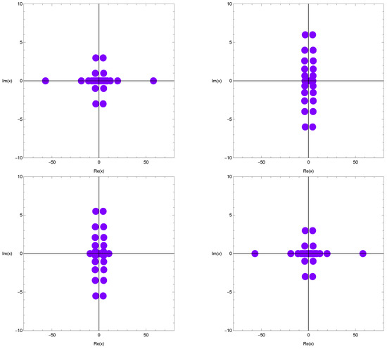
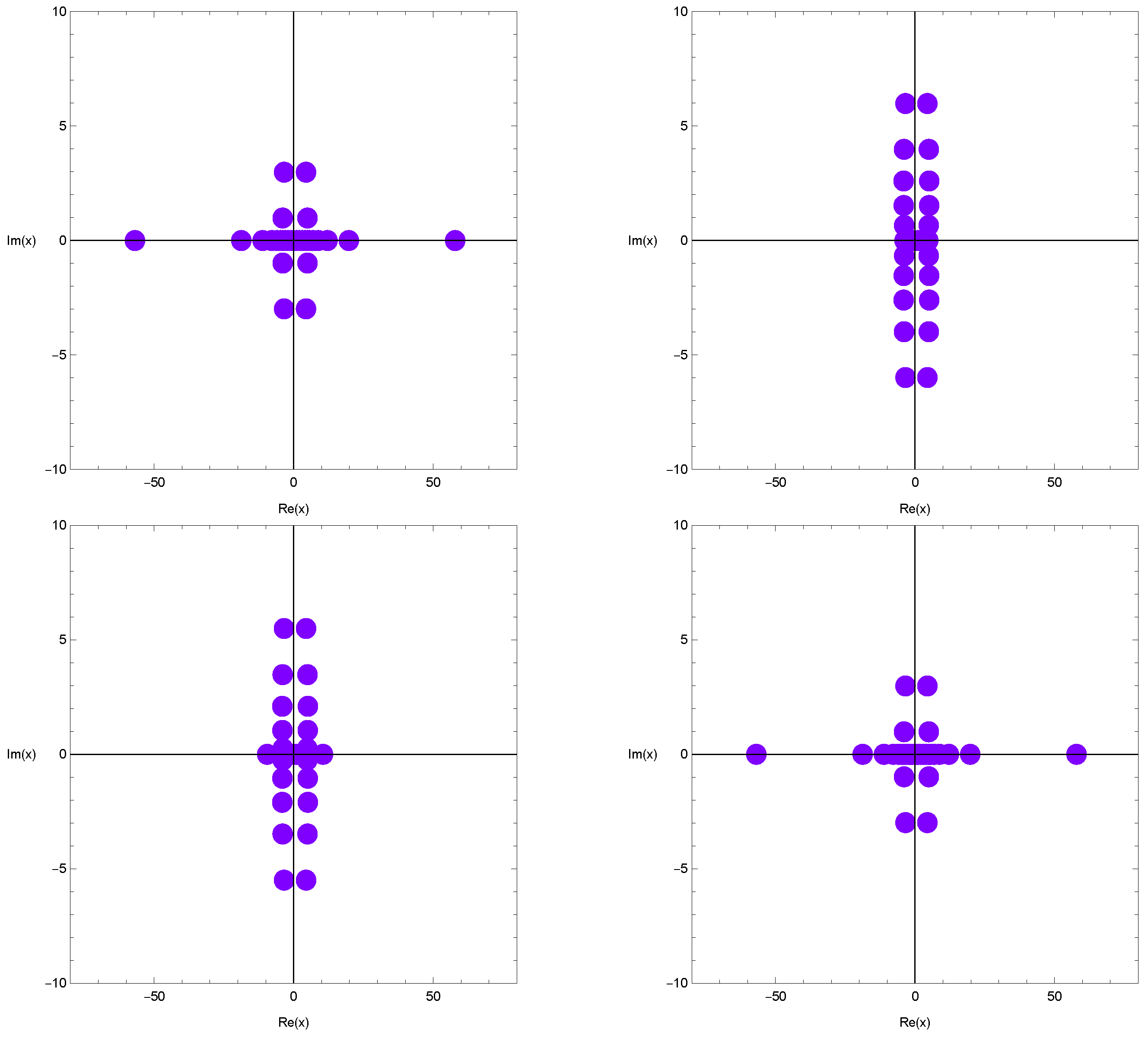
This section aims to demonstrate the benefit of using numerical investigation to support theoretical prediction and to discover a new interesting pattern of the zeros of the cosine–Euler and sine–Euler polynomials. Using a computer, a realistic study for the cosine–Euler polynomials $E_n^{(C)}(x,y)$ and sine–Euler polynomials $E_n^{(S)}(x,y)$ is very interesting. It is the aim of this paper to observe an interesting phenomenon of “scattering” of the zeros of the the cosine–Euler polynomials $E_n^{(C)}(x,y)$ and sine–Euler polynomials $E_n^{(S)}(x,y)$ in a complex plane. We investigate the beautiful zeros of the cosine–Euler and sine–Euler polynomials by using a computer. We plot the zeros of the cosine–Euler polynomials $E_n^{(C)}(x,y)$ (Figure 1).

Figure 1. Zeros of $E_n^{(C)}(x,y)$.

In Figure 1 (top-left), we choose $n=30$ and $y=-3$. In Figure 1 (top-right), we choose $n=30$ and $y=0$. In Figure 1 (bottom-left), we choose $n=30$ and $y=1/2$. In Figure 1 (bottom-right), we choose $n=30$ and $y=3$.

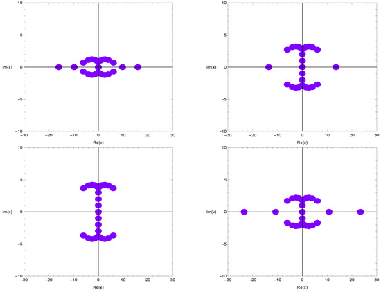
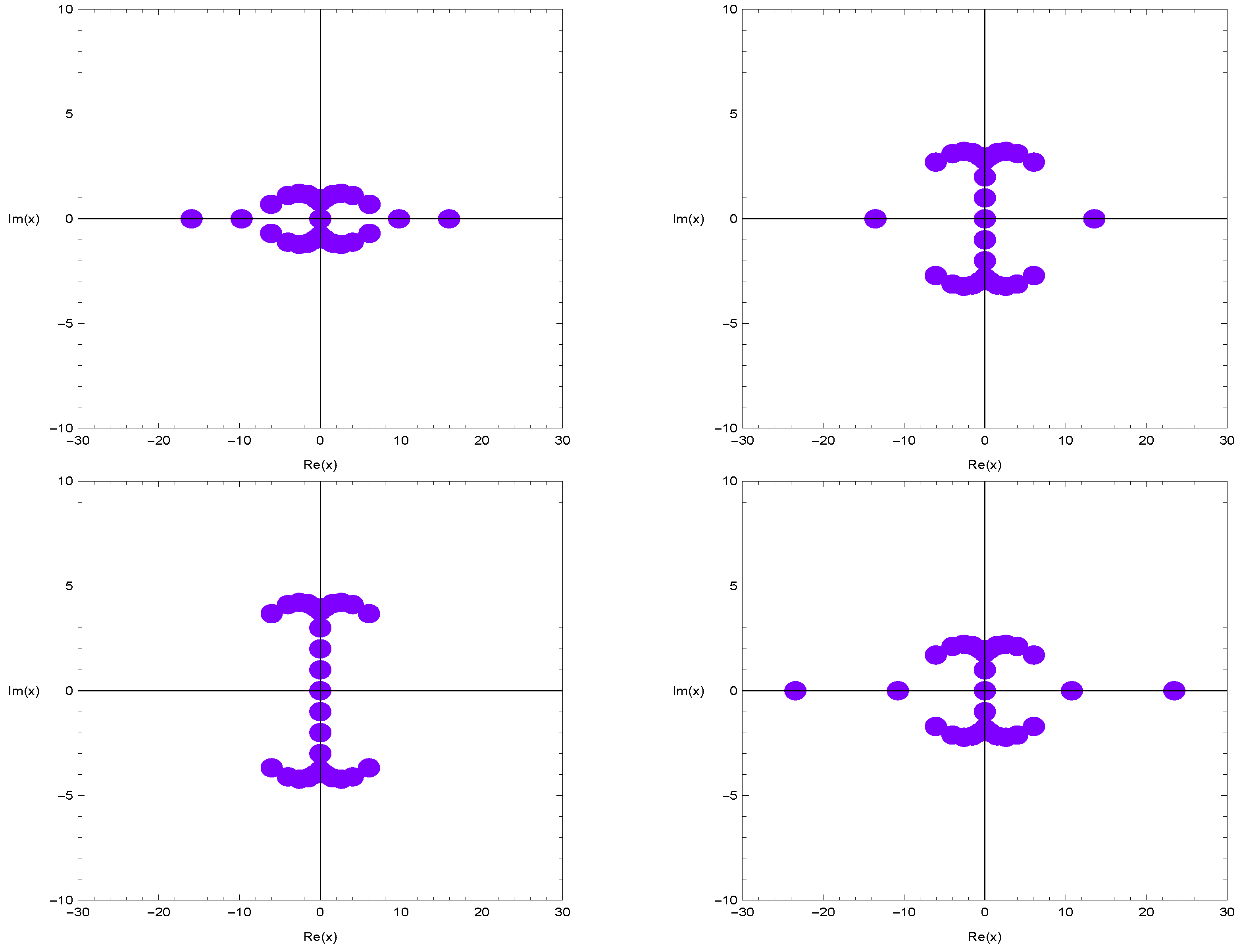
We plot the zeros of the sine–Euler polynomials $E_n^{(S)}(x,y)$ (Figure 2).

Figure 2. Zeros of $E_n^{(S)}(x,y)$.

In Figure 2 (top-left), we choose $n=30$ and $x=-3$. In Figure 2 (top-right), we choose $n=30$ and $x=-1$. In Figure 2 (bottom-left), we choose $n=30$ and $x=1$. In Figure 2 (bottom-right), we choose $n=30$ and $x=3$.

We observe that $E_n^{(C)}(x,a),x\in \mathbb{C}$ has $Re(x)=\frac{1}{2}$ reflection symmetry in addition to the usual $Im(x)=0$ reflection symmetry analytic complex functions, where $a\in \mathbb{R}$( Figure 1 and Figure 2).

Since

$$\begin{array}{cc}\hfill {\displaystyle \sum _{n=0}^{\infty }}{E}_n^{(C)}(1-x,-y){\displaystyle \frac{{(-1)}^n{t}^n}{n!}}& ={\displaystyle \frac{2}{e^{-t}+1}}{e}^{(1-x)(-t)}cosyt\hfill \\ & ={\displaystyle \frac{2}{e^t+1}}{e}^{xt}cosyt={\displaystyle \sum _{n=0}^{\infty }}{E}_n^{(C)}(x,y){\displaystyle \frac{t^n}{n!}},\hfill \end{array}$$

we obtain

$$\begin{array}{c}{E}_n^{(C)}(x,y)={(-1)}^n{E}_n^{(C)}(1-x,-y),E_n^{(C)}(x,y)={(-1)}^n{E}_n^{(C)}(1-x,y),\hfill \\ E_n^{(S)}(x,y)={(-1)}^n{E}_n^{(S)}(1-x,-y),E_n^{(S)}(x,y)={(-1)}^{n+1}{E}_n^{(S)}(1-x,y).\hfill \end{array}$$

Hence, we have the following theorem:

Theorem 15.

If $n\equiv 1(mod2)$, then

$$E_n^{(C)}(1/2,y)=0,B_n^{(C)}(1/2,y)=0,forn\in \mathbb{N}.$$

If $n\equiv 0(mod2)$, then

$$E_n^{(S)}(1/2,y)=0,B_n^{(S)}(1/2,y)=0,forn\in \mathbb{N}.$$

Our numerical results for numbers of real and complex zeros of the cosine–Euler polynomials $E_n^{(C)}(x,y)=0$ are displayed (Table 1).

Table 1. Numbers of real and complex zeros of $E_n^{(C)}(x,y)$.

Degree n	$\mathit{y}=-3$		$\mathit{y}=2$
	Real Zeros	Complex Zeros	Real Zeros	Complex Zeros
1	1	0	1	0
2	2	0	2	0
3	3	0	3	0
4	4	0	4	0
5	5	0	5	0
6	6	0	6	0
7	7	0	7	0
8	8	0	8	0
9	9	0	9	0
10	10	0	10	0

Our numerical results for numbers of real and complex zeros of the sine–Euler polynomials $E_n^{(S)}(x,y)=0$ are displayed (Table 2).

Table 2. Numbers of real and complex zeros of $E_n^{(S)}(x,y)$.

Degree n	$\mathit{x}=-3$		$\mathit{x}=1$
	Real Zeros	Complex Zeros	Real Zeros	Complex Zeros
1	1	0	1	0
2	1	0	1	0
3	3	0	3	0
4	3	0	3	0
5	5	0	5	0
6	5	0	1	4
7	7	0	7	0
8	7	0	1	6
9	9	0	9	0
10	9	0	1	8

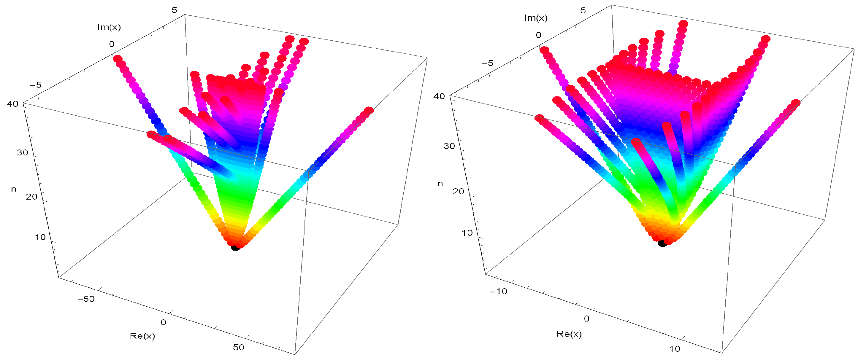
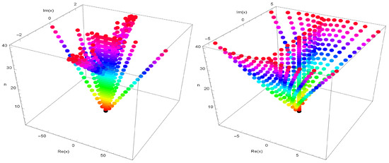
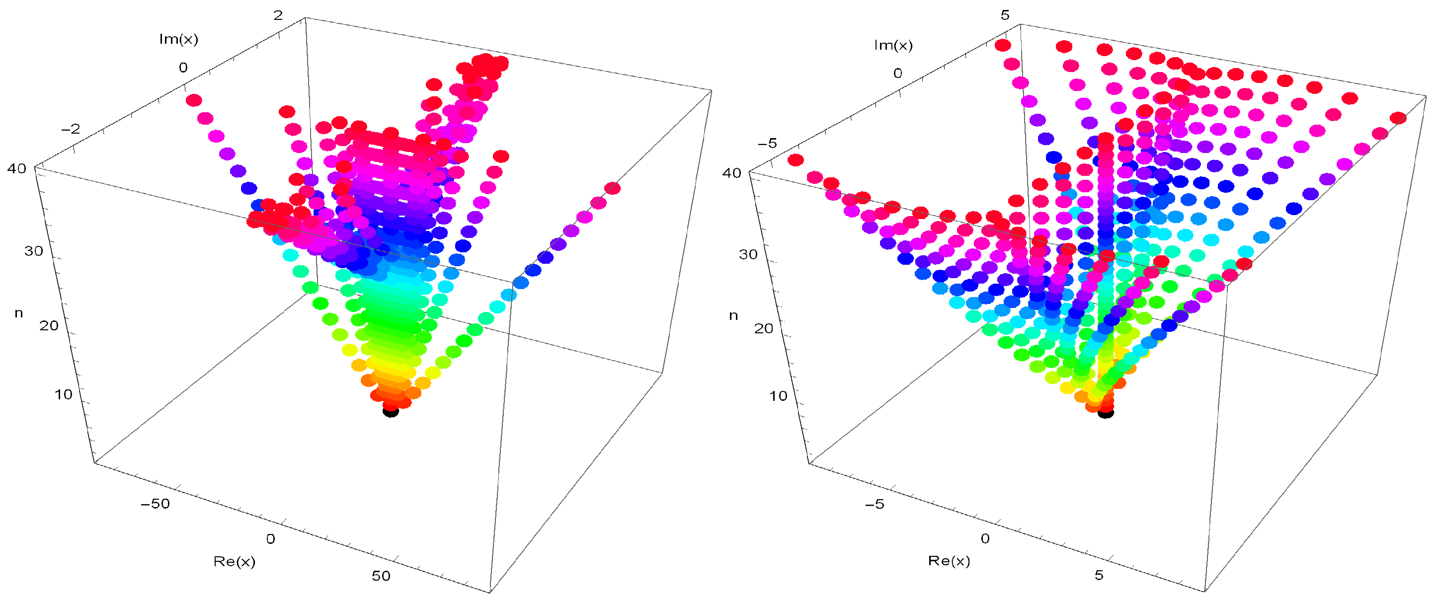
Stacks of zeros of the cosine–Euler polynomials $E_n^{(C)}(x,y)$ for $1\le n\le 40$ from a 3D structure are presented (Figure 3).

Figure 3. Stacks of zeros of $E_n^{(C)}(x,y),1\le n\le 40$.

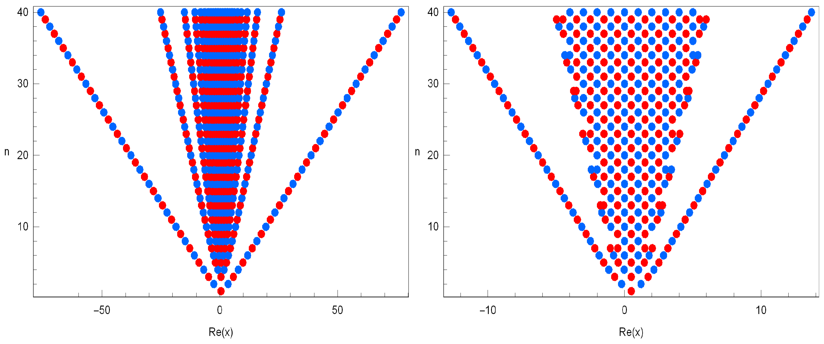
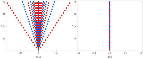
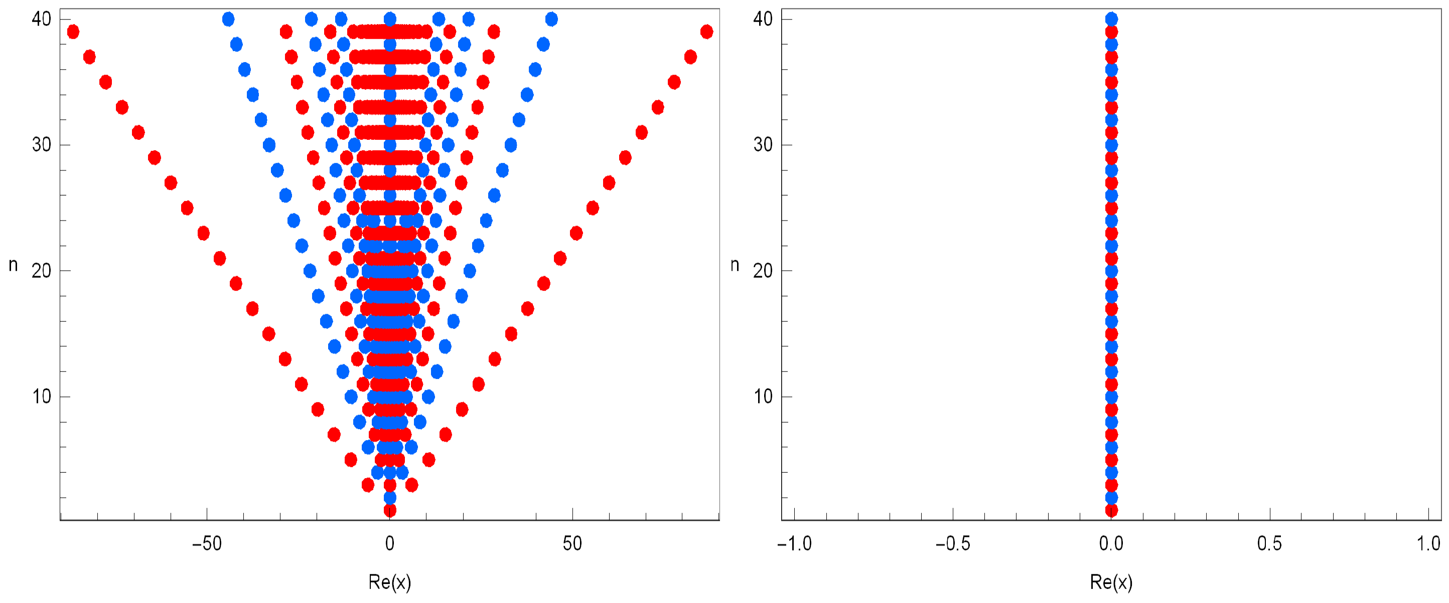
In Figure 3 (left), we choose $y=-3$. In Figure 3 (right), we choose $y=1/2$. The plot of real zeros of the cosine–Euler polynomials $E_n^{(C)}(x,y)$ for $1\le n\le 40$ structure are presented (Figure 4).

Figure 4. Real zeros of $E_n^{(C)}(x,y)$.

In Figure 4 (left), we choose $y=-3$. In Figure 4 (right), we choose $y=1/2$. Stacks of zeros of the sine–Euler polynomials $E_n^{(S)}(x,y)$ for $1\le n\le 40$ from a 3D structure are presented (Figure 5).

Figure 5. Stacks of zeros of $E_n^{(S)}(x,y),1\le n\le 40$.

In Figure 5 (left), we choose $x=-3$. In Figure 3 (right), we choose $x=1$. The plot of real zeros of the sine–Euler polynomials $E_n^{(S)}(x,y)$ for $1\le n\le 40$ structure are presented (Figure 6).

Figure 6. Real zeros of $E_n^{(S)}(x,y)$.

In Figure 6 (left), we choose $x=-3$. In Figure 6 (right), we choose $x=1$.

We observe a remarkable regular structure of the complex roots of the cosine–Euler polynomials $E_n^{(C)}(x,y)$. We also hope to verify a remarkable regular structure of the complex roots of the cosine–Euler polynomials $E_n^{(C)}(x,y)$. Next, we calculated an approximate solution satisfying $E_n^{(C)}(x,y)=0,x\in \mathbb{R}$. The results are given in Table 3.

Table 3. Approximate solutions of $E_n^{(C)}(x,-3)=0,x\in \mathbb{R}$.

Degree n	x
1				0.50000
2			−2.5414,	3.5414
3			−4.7678,	0.50000,	5.7678
4		−6.8305,	−0.82832,	1.8283,	7.8305
5		−8.8303,	−1.8336,	0.50000,	2.8336,	9.8303
6		−10.799,	−2.7017,	−0.40666,	1.4067,	3.7017,	11.799
7	−12.751,	−3.4960,	−1.1389,	0.50000,	2.1389,	4.4960,	13.751

Next, we calculated an approximate solution satisfying $E_n^{(S)}(x,y)=0,y\in \mathbb{R}$. The results are given in Table 4.

Table 4. Approximate solutionsof $E_n^{(S)}(-3,y)=0,y\in \mathbb{R}$.

Degree n	y
1	0.00000
2	0.00000
3			−6.0000,	0,	6.0000
4			−3.3912,	0,	3.3912
5		−10.687,	−2.4038,	0,	2.4038,	10.687
6		−5.9045,	−1.8630,	0,	1.8630,	5.9045
7	−15.241,	−4.1727,	−1.5184,	0,	1.5184,	4.1727,	15.241

References

- Ağyüz, E.; Acikgoz, M.; Araci, S. A symmetric identity on the q-Genocchi polynomials of higher-order under third dihedral group D3. Proc. Jangjeon Math. Soc. 2015, 18, 177–187. [Google Scholar]
- Bayad, A.; Chikhi, J. Non linear recurrences for Apostol-Bernoulli-Euler numbers of higher order. Adv. Stud. Contemp. Math. (Kyungshang) 2012, 22, 1–6. [Google Scholar]
- Carlitz, L. Recurrences for the Bernoulli and Euler numbers. II. Math. Nachr. 1965, 29, 151–160. [Google Scholar] [CrossRef] [Scilit]
- He, Y.; Kim, T. A higher-order convolution for Bernoulli polynomials of the second kind. Appl. Math. Comput. 2018, 324, 51–58. [Google Scholar] [CrossRef] [Scilit]
- Kim, D.S.; Kim, T. Some identities of Bernoulli and Euler polynomials arising from umbral calculus. Adv. Stud. Contemp. Math. (Kyungshang) 2013, 23, 159–171. [Google Scholar] [CrossRef] [Scilit]
- Kim, D.S.; Kim, T.; Kim, Y.H.; Lee, S.H. Some arithmetic properties of Bernoulli and Euler numbers. Adv. Stud. Contemp. Math. (Kyungshang) 2012, 22, 467–480. [Google Scholar]
- Kim, D.S.; Kim, T.; Kim, Y.-H.; Dolgy, D.V. A note on Eulerian polynomials associated with Bernoulli and Euler numbers and polynomials. Adv. Stud. Contemp. Math. (Kyungshang) 2012, 22, 379–389. [Google Scholar]
- Roman, S. The Umbral Calculu, Pure and Applied Mathematics, 111; Academic Press, Inc.: New York, NY, USA; Harcourt Brace Jovanovich Publishers: San Diego, CA, USA, 1984; ISBN 0-12-594380-6. [Google Scholar]
- Ryoo, C.S.; Kim, Y.H. A numerical investigation on the structure of the roots of the twisted q-Euler polynomials. Adv. Stud. Contemp. Math. (Kyungshang) 2009, 19, 131–141. [Google Scholar]
- Ryoo, C.S.; Agarwal, R.P. Some identities involving q-poly-tangent numbers and polynomials and distribution of their zeros. Adv. Differ. Equ. 2017, 213. [Google Scholar] [CrossRef] [Scilit]
- Simsek, Y. Identities on the Changhee numbers and Apostol-type Daehee polynomials. Adv. Stud. Contemp. Math. (Kyungshang) 2017, 27, 199–212. [Google Scholar]
- Srivastava, H.M.; Pintér, Á. Remarks on some relationships between the Bernoulli and Euler polynomials. Appl. Math. Lett. 2004, 17, 375–380. [Google Scholar] [CrossRef] [Scilit]
- Srivastava, H.M.; Pintér, Á. Addition theorems for the Appell polynomials and the associated classes of polynomial expansions. Aequ. Math. 2013, 85, 483–495. [Google Scholar]
- Young, P.T. Degenerate Bernoulli polynomials, generalized factorial sums, and their applications. J. Number Theor. 2008, 128, 738–758. [Google Scholar] [CrossRef] [Scilit]
© 2018 by the authors. Licensee MDPI, Basel, Switzerland. This article is an open access article distributed under the terms and conditions of the Creative Commons Attribution (CC BY) license (http://creativecommons.org/licenses/by/4.0/).