The Geometric–Natural Discrete Lindley Distribution: A One-Parameter Mixture Model with Stochastic Representation for Overdispersed Count Data

Abstract

This paper studies the geometric–natural discrete Lindley (GNDL) distribution as a structurally motivated one-parameter submodel of the published two-parameter natural discrete Lindley (TNDL) family, rather than as a new unrestricted family. The model arises from a nested geometric–NDL construction and admits equivalent geometric–negative binomial and random-sum representations. Its single parameter jointly controls the common success probability of the geometric stages and the probability of activating the two-stage component, providing parsimony at the cost of preventing these features from varying independently. We derive the main distributional and reliability properties and investigate four frequentist estimators through Monte Carlo simulation. The empirical cost of the one-parameter restriction is assessed against the unrestricted TNDL benchmark in four real-data applications and through a dedicated misspecification study. Across the applications, freeing the second parameter yields negligible log-likelihood gains, while AIC and BIC favor GNDL in every case. Misspecification is inexpensive near the GNDL restriction, whereas larger departures become increasingly detectable as sample size grows. These findings support GNDL as a tractable constrained model when its parameter coupling is compatible with the data, rather than as a universally superior alternative.

1. Introduction

Count data arise in many scientific and applied fields, including reliability, insurance, epidemiology, medicine, environmental studies, and industrial quality control. The Poisson distribution is commonly used because of its mathematical simplicity, but its equidispersion assumption can be restrictive when the empirical variance exceeds the mean. The geometric and negative binomial distributions provide classical alternatives for overdispersed counts; however, they impose particular relationships between the distributional shape, the mean, and the variance. These considerations continue to motivate the development of parsimonious discrete models that can represent overdispersion and positive skewness while retaining analytical tractability and interpretable parameter structures.

The Lindley distribution, originally introduced by Lindley [1] in a Bayesian context and subsequently studied in detail by Ghitany et al. [2], admits a mixture representation involving exponential and gamma components. This probabilistic structure has motivated several discrete Lindley-type models. Gómez-Déniz and Calderín-Ojeda [3] obtained a discrete Lindley distribution by discretizing the survival function of the continuous model and demonstrated its usefulness for overdispersed count and actuarial data. Al-Babtain et al. [4] later introduced the natural discrete Lindley (NDL) distribution by replacing the exponential and gamma components with geometric and negative binomial counterparts, respectively. Under this construction, the negative binomial component has size parameter 2, and both components share the same success probability. Related developments include the binomial–natural discrete Lindley distribution of Shafiq et al. [5], which further illustrates the role of compounding and mixture mechanisms in extending the NDL framework.

Here, “size parameter 2” is fixed and denotes the number of required successes in the negative binomial waiting-count representation; it is not an additional fitted parameter. Thus, the negative binomial component counts the total number of unsuccessful trials before the second success and is equivalently the sum of two independent geometric failure-count variables with the same success probability.

Although these models enrich the discrete Lindley family, a relevant modeling question is whether the relative contribution of one-stage and two-stage waiting mechanisms can be modified while preserving a fully discrete one-parameter specification. Introducing an unrestricted mixing parameter would provide additional flexibility, but it would also increase model complexity and weaken the direct dependence between the component distributions and the mixing mechanism. The present study instead considers a parameter-dependent mixture of the geometric and NDL distributions in which the same model parameter governs both the component waiting behavior and the mixing probabilities.

This construction leads to the geometric–natural discrete Lindley (GNDL) distribution. Expanding the NDL component shows that the GNDL model possesses an equivalent two-component representation involving a geometric distribution and a negative binomial distribution with size parameter 2. In this equivalent representation, the probability of activating the two-stage negative binomial mechanism is determined by the common model parameter and is smaller than the corresponding two-stage weight in the NDL distribution. Thus, in the mixture-weight sense, the GNDL model provides an intermediate one-parameter structure between the geometric and NDL distributions without introducing an additional free mixing parameter.

The equivalent representation also supplies a direct latent-stage interpretation. An observation may be generated by a single geometric waiting stage or by the sum of two independent geometric stages, which follows a negative binomial distribution with size parameter 2. The model parameter therefore jointly controls the success probability within the stages and the probability that the latent second stage is activated. This interpretation may be relevant to stylized reliability, maintenance, or inspection processes in which completion requires either one successful stage or two successive successful stages. It should not, however, be interpreted as asserting that every data set fitted by the GNDL distribution must literally arise from such a mechanism. Moreover, the one-parameter formulation imposes a structural restriction because the stage-specific success probability and the stage-activation probability cannot vary independently. Throughout this paper, the geometric variable counts the number of unsuccessful trials before the first success, the negative binomial variable counts the number of unsuccessful trials before the second success, the support is ${\mathbb{N}}_0$, and the common parameter satisfies $0 < \alpha < 1$.

The direct geometric–negative binomial representation also places GNDL within the existing two-parameter literature. Al-Babtain et al. [4] introduced the two-parameter natural discrete Lindley (TNDL) family, with their one-parameter NDL model obtained as a special case, and the GNDL law corresponds to a specific one-dimensional restriction of TNDL. A related two-parameter Poisson–Lindley formulation was given by Shanker and Mishra [6]; on the positive-parameter region relevant to a convex geometric–negative binomial mixture, it is a one-to-one reparameterization of the same interior geometric–negative-binomial family. The resulting linear-geometric form can also be viewed as a weighted geometric distribution in the sense of Fisher [7], Rao [8], and Patil and Rao [9]. The exact probability mass functions, parameter mappings, and containment relations are established later in Section 2.

Accordingly, the contribution of the present work does not lie in introducing a previously unknown unrestricted two-parameter family. Rather, it lies in the systematic study of the specific one-parameter coupling induced by the nested geometric–NDL construction, together with its stochastic interpretation, mathematical properties, estimation procedures, and an explicit assessment of the empirical cost of imposing that restriction. The coupling gains parsimony by linking the within-stage success behavior to the probability of activating the two-stage component, but it prevents these two features from being adjusted independently.

The principal contributions of this study are as follows. First, the specific GNDL restriction is characterized through its nested geometric–NDL construction, equivalent geometric–negative binomial mixture, and latent-stage/random-sum representations, and its position within the relevant existing two-parameter families is established explicitly. Second, its main distributional properties are derived, including the probability-generating and moment-generating functions, moments, dispersion measures, shape characteristics, survival and hazard functions, stochastic-ordering relations, and aging properties. Third, four estimation procedures are investigated: maximum likelihood, method of moments, method of proportions, and minimum chi-square estimation, with finite-sample behavior examined through an extensive Monte Carlo study. Fourth, the empirical cost of the one-parameter restriction is assessed using four real data sets with the unrestricted TNDL model as the natural benchmark and through a dedicated misspecification study over the encompassing two-parameter family. The empirical comparisons are interpreted in terms of competitive goodness of fit and parsimony rather than universal superiority.

The remainder of the paper is organized as follows. Section 2 develops the stochastic construction and generative interpretation of GNDL and establishes its exact position within the relevant existing two-parameter families. Section 3 gives its formal definition and principal distributional functions. Section 4, Section 5 and Section 6 develop its mathematical properties, reliability and aging characteristics, and stochastic-ordering results. Section 7 discusses the four estimation methods and reports the Monte Carlo simulation study. Section 8 presents the real-data applications, the unrestricted benchmark, and the misspecification assessment. Section 9 concludes the paper.

2. Theoretical Motivation and Generative Interpretation of the GNDL Distribution

The GNDL construction builds on the natural discrete Lindley framework. The continuous Lindley distribution admits a mixture representation involving exponential and gamma components, the latter having shape parameter 2. Al-Babtain et al. [4] obtained the natural discrete Lindley (NDL) distribution by replacing these components with their geometric and negative binomial analogues and retaining a common success probability. Under the notation adopted here, $\alpha \in \left(0,1\right)$, and the support is ${\mathbb{N}}_0=\{0,1,2,\dots \}$. The geometric component counts unsuccessful trials before the first success, whereas the negative binomial component with size parameter 2 counts unsuccessful trials before the second success. Their probability mass functions are

$$p_G\left(y;\alpha \right)=\alpha {\left(1-\alpha \right)}^y, p_{\mathrm{N}\mathrm{B}2}\left(y;\alpha \right)=\left(y+1\right){\alpha }^2{\left(1-\alpha \right)}^y, y\in {\mathbb{N}}_0.$$

The NDL probability mass function can therefore be written as

$$p_{\mathrm{N}\mathrm{D}\mathrm{L}}\left(y;\alpha \right)={\displaystyle \frac{\alpha }{1+\alpha }}{p}_G\left(y;\alpha \right)+{\displaystyle \frac{1}{1+\alpha }}{p}_{\mathrm{N}\mathrm{B}2}\left(y;\alpha \right)={\displaystyle \frac{{\alpha }^2\left(y+2\right){\left(1-\alpha \right)}^y}{1+\alpha }}.$$

The GNDL construction considered here applies the same parameter-dependent mixing rule once more, now combining the geometric and NDL distributions:

$$p_{\mathrm{G}\mathrm{N}\mathrm{D}\mathrm{L}}\left(y;\alpha \right)={\displaystyle \frac{\alpha }{1+\alpha }}{p}_G\left(y;\alpha \right)+{\displaystyle \frac{1}{1+\alpha }}{p}_{\mathrm{N}\mathrm{D}\mathrm{L}}\left(y;\alpha \right).$$

Proposition 1.

For every $\alpha \in \left(0,1\right)$, the preceding nested geometric–NDL representation is equivalent to the following direct two-component mixture

$$p_{GNDL}\left(y;\alpha \right)=w_G\left(\alpha \right)p_G\left(y;\alpha \right)+w_2\left(\alpha \right)p_{NB2}\left(y;\alpha \right).$$

where

$$w_G\left(\alpha \right)={\displaystyle \frac{\alpha \left(\alpha +2\right)}{{\left(1+\alpha \right)}^2}}, w_2\left(\alpha \right)={\displaystyle \frac{1}{{\left(1+\alpha \right)}^2}}.$$

Consequently, its marginal probability mass function is

$$p_{\mathrm{G}\mathrm{N}\mathrm{D}\mathrm{L}}\left(y;\alpha \right)={\displaystyle \frac{{\alpha }^2\left(y+3+\alpha \right){\left(1-\alpha \right)}^y}{{\left(1+\alpha \right)}^2}}, y\in {\mathbb{N}}_0.$$

Proof. 

Substitution of the NDL representation into the nested geometric–NDL construction gives

$${\displaystyle \frac{\alpha }{1+\alpha }}{p}_G+{\displaystyle \frac{1}{1+\alpha }}\left({\displaystyle \frac{\alpha }{1+\alpha }}{p}_G+{\displaystyle \frac{1}{1+\alpha }}{p}_{\mathrm{N}\mathrm{B}2}\right)={\displaystyle \frac{\alpha \left(\alpha +2\right)}{{\left(1+\alpha \right)}^2}}{p}_G+{\displaystyle \frac{1}{{\left(1+\alpha \right)}^2}}{p}_{\mathrm{N}\mathrm{B}2}.$$

Both coefficients are strictly positive for $\alpha \in \left(0,1\right)$, and

$$w_G\left(\alpha \right)+w_2\left(\alpha \right)={\displaystyle \frac{\alpha \left(\alpha +2\right)+1}{{\left(1+\alpha \right)}^2}}=1.$$

Thus, the preceding expression is a valid finite mixture. Substituting the component mass functions into it yields the displayed marginal probability mass function. □

The reduction in Proposition 1 replaces the nested geometric–NDL construction by a single latent indicator. The two-stage weight is not an additional free parameter. Indeed,

$$w_2^{\prime }\left(\alpha \right)=-{\displaystyle \frac{2}{{\left(1+\alpha \right)}^3}}<0, w_G^{\prime }\left(\alpha \right)={\displaystyle \frac{2}{{\left(1+\alpha \right)}^3}}>0.$$

Hence, increasing $\alpha$ simultaneously shortens the geometric waiting times and shifts mixture mass toward the one-stage component. This coupling preserves a one-parameter model, but it is also a structural restriction because the within-stage success probability and the probability of activating the second stage cannot vary independently.

Proposition 2.

For every  $\alpha \in \left(0,1\right)$, the GNDL family is distinct from both the geometric and NDL families. Specifically, there is no $\beta \in \left(0,1\right)$ such that $p_{\mathrm{GNDL}}\left(y;\alpha \right)=p_G\left(y;\beta \right)$ for all $y\in {\mathbb{N}}_0$, and there is no $\beta \in \left(0,1\right)$ such that $p_{\mathrm{GNDL}}\left(y;\alpha \right)=p_{\mathrm{NDL}}\left(y;\beta \right)$ for all $y\in {\mathbb{N}}_0$.

Proof. 

From Proposition 1, the successive-probability ratio of the GNDL distribution is ${\displaystyle \frac{p_{\mathrm{GNDL}}\left(y+1;\alpha \right)}{p_{\mathrm{GNDL}}\left(y;\alpha \right)}}=\left(1-\alpha \right){\displaystyle \frac{y+4+\alpha }{y+3+\alpha }}$. For a geometric distribution with parameter $\beta$, ${\displaystyle \frac{p_G\left(y+1;\beta \right)}{p_G\left(y;\beta \right)}}=1-\beta$, which is constant in $y$; hence, no geometric distribution can coincide with $\mathrm{GNDL}\left(\alpha \right)$. For $\mathrm{NDL}\left(\beta \right)$, ${\displaystyle \frac{p_{\mathrm{NDL}}\left(y+1;\beta \right)}{p_{\mathrm{NDL}}\left(y;\beta \right)}}=\left(1-\beta \right){\displaystyle \frac{y+3}{y+2}}$. If $\mathrm{GNDL}\left(\alpha \right)$ and $\mathrm{NDL}\left(\beta \right)$ were identical, equality of these ratios for all $y$ and passage to the limit $y\to \mathrm{\infty }$ would give $\beta =\alpha$. Substitution would then require $\left(y+4+\alpha \right)\left(y+2\right)=\left(y+3+\alpha \right)\left(y+3\right)$, but the difference between the two sides is $-\left(1+\alpha \right)\ne 0$, a contradiction for $0<\alpha <1$. Hence, the GNDL family is not a reparameterization of either the geometric or the NDL family. This completes the proof. □

Proposition 3.

Let  $X_1$ and  $X_2$  be independent geometric random variables with success probability  $\alpha$, and let  $Z$  be an independent Bernoulli indicator. Define the random number of stages by  $N=1+Z$. If

$$P\left(Z=1\right)={\pi }_{\alpha }={\displaystyle \frac{1}{{\left(1+\alpha \right)}^2}}, P\left(Z=0\right)=1-{\pi }_{\alpha }.$$

and

$$N=1+Z, Y={\displaystyle \sum _{j=1}^N}{X}_j=X_1+Z{X}_2.$$

then  $Y$  has the marginal probability mass function displayed in Proposition 1.

Proof. 

Conditionally on $Z=0\hspace{0.33em}\left(N=1\right)$, one has $Y={\sum }_{j=1}^N{X}_j=X_1+Z{X}_2$ = $X_1$, so the conditional distribution is geometric. Conditionally on $Z=1\hspace{0.33em}\left(N=2\right)$, one has $Y={\sum }_{j=1}^N{X}_j=X_1+Z{X}_2$ = $X_1+X_2$. For every nonnegative integer $y$, convolution gives

$$P\left(X_1+X_2=y\right)={\displaystyle \sum _{x=0}^y}\alpha {\left(1-\alpha \right)}^x\alpha {\left(1-\alpha \right)}^{y-x}=\left(y+1\right){\alpha }^2{\left(1-\alpha \right)}^y=p_{\mathrm{N}\mathrm{B}2}\left(y;\alpha \right).$$

The law of total probability therefore reproduces the direct mixture in Proposition 1, proving the result. □

Proposition 3 supplies an exact generation scheme: draw $Z$, set $N=1+Z$, generate $X_1,\dots ,X_N$, and return $Y={\sum }_{j=1}^N{X}_j=X_1+Z{X}_2$. It also makes explicit that the negative binomial component corresponds to the accumulated number of unsuccessful trials over two geometric stages.

Corollary 1.

Under the representation in Proposition 3, the conditional probabilities of the latent pathway are

$${\tau }_{\alpha }\left(y\right)=P\left(Z=1\mid Y=y\right)={\displaystyle \frac{y+1}{y+3+\alpha }}, P\left(Z=0\mid Y=y\right)={\displaystyle \frac{2+\alpha }{y+3+\alpha }}.$$

Proof. 

Bayes’ formula, together with the direct mixture and marginal probability mass function in Proposition 1, gives

$$P\left(Z=1\mid Y=y\right)={\displaystyle \frac{{\pi }_{\alpha }{p}_{\mathrm{N}\mathrm{B}2}\left(y;\alpha \right)}{p_{\mathrm{G}\mathrm{N}\mathrm{D}\mathrm{L}}\left(y;\alpha \right)}}={\displaystyle \frac{y+1}{y+3+\alpha }}.$$

after cancellation of the common factors. The complementary probability follows immediately. □

Moreover, the two-stage probability and its associated conditional odds satisfy

$${\tau }_{\alpha }\left(y+1\right)-{\tau }_{\alpha }\left(y\right)={\displaystyle \frac{2+\alpha }{\left(y+3+\alpha \right)\left(y+4+\alpha \right)}}>0, {\displaystyle \frac{{\tau }_{\alpha }\left(y\right)}{1-{\tau }_{\alpha }\left(y\right)}}={\displaystyle \frac{y+1}{2+\alpha }}.$$

Thus, within the fitted latent representation, larger counts are assigned progressively greater conditional probability of arising from the two-stage component; in fact, the associated odds increase linearly with y, while the posterior two-stage probability approaches one as y tends to infinity. These are model-based allocation probabilities, not evidence that the observations belong to physically distinct populations.

From an applied perspective, the representation may describe processes in which completion requires either one successful stage or two successful stages. In a reliability or maintenance setting, $Y$ may represent the total number of unsuccessful intervention attempts before a unit is returned to service. The one-stage pathway ends after a successful repair, whereas the two-stage pathway requires a successful repair followed by a successful verification or calibration stage. Here, $X_1$ and $X_2$ count the unsuccessful attempts in the two stages and $Z$ indicates whether the second stage is required. This is a coherent stochastic interpretation of the model; it does not imply that every data set fitted by the GNDL distribution must literally arise from that mechanism.

Consequently, the nested geometric–NDL formulation preserves the connection with the natural discrete Lindley family, while the equivalent geometric–negative binomial mixture, the random-sum representation, and the conditional latent-stage probabilities provide an explicit latent-stage basis for the model. The relationship of this construction to the relevant existing two-parameter families is established next.

Position Within Existing Two-Parameter Families

To make the structural restriction explicit, consider first the unrestricted two-component geometric–negative binomial mixture

$$f\left(y;\rho ,\omega \right)=\left(1-\omega \right)\rho {\left(1-\rho \right)}^y+\omega \left(y+1\right){\rho }^2{\left(1-\rho \right)}^y, y\in {\mathbb{N}}_0, 0<\rho <1, 0\le \omega \le 1.$$

The first parameter is the common success probability of the geometric and negative binomial (size 2) components, whereas the second is the probability assigned to the two-stage negative binomial component. Thus, the two parameters control distinct distributional features. After collecting terms, the probability mass is a linear function of the count multiplied by a geometric factor, so this family can also be viewed as a weighted geometric distribution in the sense of Fisher [7], Rao [8], and Patil and Rao [9].

The TNDL distribution of Al-Babtain et al. [4] provides a parameterization of the interior of this family, with probability mass function

$$p_{\mathrm{T}\mathrm{N}\mathrm{D}\mathrm{L}}\left(y;\theta ,\kappa \right)={\displaystyle \frac{{\theta }^2}{\theta +\kappa }}\left[1+\kappa \left(y+1\right)\right]{\left(1-\theta \right)}^y,\hspace{1em}y\in {\mathbb{N}}_0,\hspace{1em}0<\theta <1,\hspace{1em}\kappa >0.$$

Its geometric and negative binomial mixing weights are, respectively,

$$\left({\displaystyle \frac{\theta }{\theta +\kappa }},{\displaystyle \frac{\kappa }{\theta +\kappa }}\right)$$

Hence, TNDL is exactly the interior of the preceding unrestricted mixture under the explicit mapping

$$\rho =\theta ,\hspace{1em}\hspace{1em}\omega ={\displaystyle \frac{\kappa }{\theta +\kappa }},\hspace{1em}\hspace{1em}0<\rho <1,\hspace{1em}\hspace{1em}0<\omega <1$$

Conversely, the inverse mapping on the interior is

$$\theta =\rho ,\hspace{1em}\hspace{1em}\kappa ={\displaystyle \frac{\rho \omega }{1-\omega }},\hspace{1em}\hspace{1em}0<\rho <1,\hspace{1em}\hspace{1em}0<\omega <1$$

Their one-parameter NDL model is recovered by fixing the second TNDL parameter at one. For the GNDL construction, the restriction is

$$\theta =\alpha ,\hspace{1em}\hspace{1em}\kappa ={\left(\alpha +2\right)}^{-1}.$$

Substitution into the TNDL probability mass function reproduces exactly the GNDL marginal probability mass function obtained in Proposition 1. Combining the same identification with the unrestricted mixture coordinates yields the deterministic GNDL mixing relation

$$\omega ={\omega }_{GNDL}\left(\rho \right)={\displaystyle \frac{1}{{\left(1+\rho \right)}^2}}$$

Thus, GNDL is a one-dimensional curve inside the interior of the published TNDL family, rather than a new unrestricted two-parameter family.

A second exact literature connection is provided by the two-parameter Poisson–Lindley distribution of Shanker and Mishra [6]. On the positive-parameter region used for the convex-mixture comparison, its probability mass function is

$$p_{\mathrm{S}\mathrm{M}}\left(y;\xi ,\eta \right)={\displaystyle \frac{{\eta }^2}{{\left(1+\eta \right)}^{y+2}}}\left(1+{\displaystyle \frac{\xi +y}{1+\xi \eta }}\right),\hspace{1em}y\in {\mathbb{N}}_0,\hspace{1em}\xi >0,\hspace{1em}\eta >0.$$

On the positive-parameter subregion relevant to a convex mixture, this model maps exactly onto the TNDL parameterization through

$$\theta ={\displaystyle \frac{\eta }{1+\eta }},\hspace{1em}\hspace{1em}\kappa ={\displaystyle \frac{1}{\xi \left(1+\eta \right)}},\hspace{1em}\hspace{1em}\xi >0.$$

The inverse transformation on this region is

$$\eta ={\displaystyle \frac{\theta }{1-\theta }},\hspace{1em}\hspace{1em}\xi ={\displaystyle \frac{1-\theta }{\kappa }}.$$

Direct substitution verifies that the Shanker–Mishra probability mass function then reduces to the TNDL form displayed above. Thus, on this positive convex-mixture region, the two published two-parameter formulations are one-to-one reparameterizations of the same family. The full Shanker–Mishra parameter domain is broader than this positive region, so the equivalence asserted here is restricted to the region relevant to the convex-mixture representation. The GNDL restriction corresponds in the Shanker–Mishra parameterization to

$$\eta ={\displaystyle \frac{\alpha }{1-\alpha }},\hspace{1em}\hspace{1em}\xi =\left(1-\alpha \right)\left(\alpha +2\right),\hspace{1em}\hspace{1em}0<\alpha <1.$$

Therefore, GNDL is a one-dimensional curve inside both the published TNDL family and the positive-parameter convex-mixture region of the Shanker–Mishra two-parameter Poisson–Lindley model. The underlying two-parameter Lindley model is due to Shanker and Mishra [10], while Sankaran [11] introduced the classical one-parameter Poisson–Lindley model.

The one-parameter restriction has a clear interpretation and a clear cost. Increasing the common success probability shortens the waiting-time components and, because

$${\displaystyle \frac{d{\omega }_{GNDL}\left(\rho \right)}{d\rho }}=-{\displaystyle \frac{2}{{\left(1+\rho \right)}^3}}<0$$

simultaneously reduces the probability of activating the two-stage component. The unrestricted mixture can vary the success probability and the stage-activation probability separately, whereas GNDL ties them together. For the unrestricted mixture, let $Y_{\rho ,\omega }$ denote a random variable following this mixture. Its mean and variance are

$$\mathbb{E}\left(Y_{\rho ,\omega }\right)={\displaystyle \frac{\left(1+\omega \right)\left(1-\rho \right)}{\rho }}$$

$$\mathrm{V}\mathrm{a}\mathrm{r}\left(Y_{\rho ,\omega }\right)={\displaystyle \frac{\left(1-\rho \right)\left[1+\omega +\omega \left(1-\omega \right)\left(1-\rho \right)\right]}{{\rho }^2}}$$

Consequently, dispersion is determined jointly by the two unrestricted coordinates, whereas under GNDL it becomes a function of the single GNDL parameter. The same coupling jointly determines the zero probability, tail concentration, mean, variance, dispersion, and mixing weight. Estimation of GNDL can therefore be viewed as fitting the observed distribution along a one-dimensional structural curve rather than estimating stage success and stage activation separately. The gain is parsimony and a fully specified stochastic mechanism; the cost is that data requiring a different combination of these two features cannot be represented exactly. The unrestricted TNDL/2P-PLD benchmark and the misspecification study quantify this cost rather than assuming that it is negligible.

With the construction and its position within the existing two-parameter families now established, the next section gives the formal definition and basic distributional functions of GNDL.

3. Definition and Distributional Formulation of the GNDL Distribution

Following the construction, stochastic representation, and family positioning established in Section 2, this section takes the resulting GNDL probability mass function as the formal definition of the model and presents its basic distributional functions.

Definition 1.

A non-negative integer-valued random variable  $Y$ is said to follow the geometric–natural discrete Lindley distribution with parameter  $\alpha$, denoted by  $Y\sim GNDL\left(\alpha \right)$, if its probability mass function is

$$p\left(y;\alpha \right)={\displaystyle \frac{{\alpha }^2\left(3+\alpha +y\right){\left(1-\alpha \right)}^y}{{\left(1+\alpha \right)}^2}}, y\in {\mathbb{N}}_0, 0<\alpha <1.$$

(1)

The expression in Equation (1) is the common marginal probability mass function produced by both the nested geometric–NDL construction and the equivalent geometric–negative binomial latent-stage representation established in Section 2.

The corresponding cumulative distribution function is

$$F\left(y;\alpha \right)=P\left(Y\le y\right)={\displaystyle \sum _{k=0}^y}p\left(k;\alpha \right)=1-{\displaystyle \frac{\left(1+3\alpha +{\alpha }^2+\alpha y\right){\left(1-\alpha \right)}^{y+1}}{{\left(1+\alpha \right)}^2}}, y\in {\mathbb{N}}_0.$$

(2)

For completeness, Equation (2) can be verified directly from Equation (1). Writing $q=1-\alpha$ and using the finite-series identities

$${\displaystyle \sum _{k=0}^y}{q}^k={\displaystyle \frac{1-q^{y+1}}{\alpha }}, {\displaystyle \sum _{k=0}^y}k\hspace{0.17em}{q}^k={\displaystyle \frac{q-\left(y+1\right)q^{y+1}+y{q}^{y+2}}{{\alpha }^2}},$$

gives

$${\displaystyle \sum _{k=0}^y}p\left(k;\alpha \right)=1-{\displaystyle \frac{\left(1+3\alpha +{\alpha }^2+\alpha y\right){\left(1-\alpha \right)}^{y+1}}{{\left(1+\alpha \right)}^2}}.$$

Equivalently, $F\left(y;\alpha \right)-F\left(y-1;\alpha \right)=p\left(y;\alpha \right)$ for every $y\in {\mathbb{N}}_0$, with $F\left(-1;\alpha \right)=0$.

For $y<0$, $F\left(y;\alpha \right)=0$.

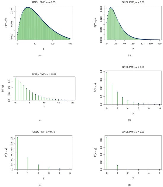
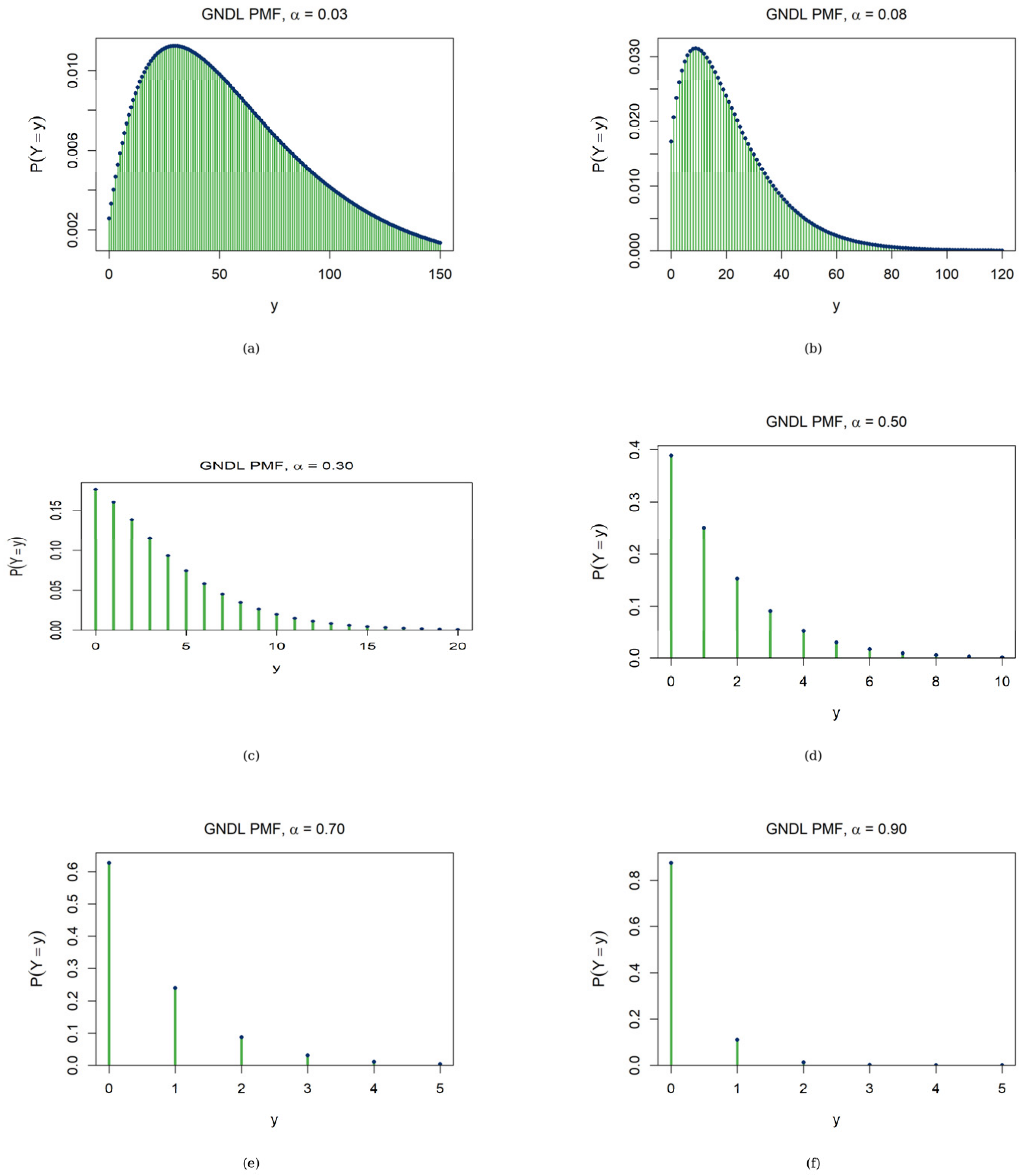
Figure 1 displays selected probability mass functions of the GNDL distribution. At the smaller parameter values shown, the probability mass extends over a wider range of counts and the right tail decreases more gradually; when $\alpha$ is sufficiently small, the mode may occur at a positive integer. As $\alpha$ increases, the probability mass becomes increasingly concentrated near zero. In particular, the probability mass function is non-increasing for $\alpha \ge \sqrt{5}-2$; at $\alpha =\sqrt{5}-2$, the first two probabilities are equal, whereas it is strictly decreasing for $\alpha >\sqrt{5}-2$. These plots illustrate the effect of $\alpha$ on the concentration and modal location of the distribution within the one-parameter structure described in Section 2. The graphical patterns are consistent with the formal unimodality and mode results derived in the subsequent analysis.

Figure 1. Probability mass function (PMF) of the GNDL distribution for selected values of $\alpha$: (a) $\alpha$ = 0.03; (b) $\alpha$ = 0.08; (c) $\alpha$ = 0.30; (d) $\alpha$= 0.50; (e) α = 0.70; (f) $\alpha$ = 0.90.

4. Mathematical and Probabilistic Properties of the GNDL Distribution

This section develops the principal mathematical and probabilistic characteristics of the GNDL distribution, including its generating functions, moments, shape measures, and index of dispersion. These results provide an analytical description of the distributional behavior induced by the parameter $\alpha$.

4.1. Generating Functions, Moments, and Shape Characteristics

Theorem 1.

If  $Y\sim GNDL\left(\alpha \right)$, where  $0<\alpha <1$, then the moment-generating function of  $Y$  is given by

$$M_Y\left(t\right)={\displaystyle \frac{{\alpha }^3+3{\alpha }^2+e^t\left({\alpha }^4+{\alpha }^3-2{\alpha }^2\right)}{{\left[1+\alpha +e^t\left({\alpha }^2-1\right)\right]}^2}}, t<-log\left(1-\alpha \right).$$

(3)

Proof. 

From the equivalent geometric–negative binomial mixture representation established in Section 2, the mixing weights of the geometric and negative binomial components are, respectively,

$$w_G(\alpha )={\displaystyle \frac{\alpha (\alpha +2)}{{(1+\alpha )}^2}}, w_2(\alpha )={\displaystyle \frac{1}{{(1+\alpha )}^2}}.$$

Under the adopted parameterization, the moment-generating functions of the geometric distribution and the negative binomial distribution with size parameter 2 are

$$M_G\left(t\right)={\displaystyle \frac{\alpha }{1-\left(1-\alpha \right)e^t}} \mathrm{and} M_{NB}\left(t\right)={\left[{\displaystyle \frac{\alpha }{1-\left(1-\alpha \right)e^t}}\right]}^2,$$

provided that $\left(1-\alpha \right)e^t<1$, equivalently $t<-\mathrm{l}\mathrm{o}\mathrm{g}\left(1-\alpha \right)$. Therefore,

$$M_Y\left(t\right)=w_G\left(\alpha \right)M_G\left(t\right)+w_2\left(\alpha \right)M_{NB}\left(t\right),$$

and hence

$$M_Y\left(t\right)={\displaystyle \frac{{\alpha }^2\left(\alpha +2\right)}{{\left(1+\alpha \right)}^2\left[1-\left(1-\alpha \right)e^t\right]}}+{\displaystyle \frac{{\alpha }^2}{{\left(1+\alpha \right)}^2{\left[1-\left(1-\alpha \right)e^t\right]}^2}}.$$

Combining the two terms over a common denominator and simplifying gives Equation (3). This completes the proof. □

Corollary 2.

The probability-generating function of a random variable  $Y$ following the GNDL distribution is

$$G_Y\left(s\right)=\mathbb{E}\left(s^Y\right)={\displaystyle \frac{{\alpha }^3+3{\alpha }^2+s\left({\alpha }^4+{\alpha }^3-2{\alpha }^2\right)}{{\left[1+\alpha +s\left({\alpha }^2-1\right)\right]}^2}}.$$

The probability-generating function is finite for $\left|s\right|<{\displaystyle \frac{1}{1-\alpha }}$.

This expression follows from Equation (3) by replacing $e^t$ with $s$, or equivalently by setting $t=\mathrm{l}\mathrm{o}\mathrm{g}s$ whenever $s>0$. Based on Equation (3), the $r$th non-central moment of the GNDL distribution is obtained from

$${{\mu }_r}^{\prime }=\mathbb{E}\left(Y^r\right)=M_Y^{\left(r\right)}\left(0\right), r=1,2,\dots .$$

In particular, the mean and variance are

$$\mathbb{E}\left(Y\right)={\displaystyle \frac{2-{\alpha }^2-{\alpha }^3}{\alpha {\left(1+\alpha \right)}^2}},$$

(4)

and

$$\mathrm{V}\mathrm{a}\mathrm{r}\left(Y\right)={\displaystyle \frac{\left(1-\alpha \right)\left(2+8\alpha +6{\alpha }^2+3{\alpha }^3+{\alpha }^4\right)}{{\alpha }^2{\left(1+\alpha \right)}^4}}.$$

(5)

An independent verification of the variance follows from the equivalent geometric–negative binomial representation. With $w_2\left(\alpha \right)={\left(1+\alpha \right)}^{-2}$ denoting the negative binomial mixing weight, the law of total variance gives

$$\mathrm{V}\mathrm{a}\mathrm{r}\left(Y\right)={\displaystyle \frac{1-\alpha }{{\alpha }^2}}\left(1+w_2\left(\alpha \right)\right)+w_2(\alpha )\left(1-w_2\left(\alpha \right)\right){\displaystyle \frac{{\left(1-\alpha \right)}^2}{{\alpha }^2}}.$$

Substitution of $w_2\left(\alpha \right)={\left(1+\alpha \right)}^{-2}$ and simplification reproduce Equation (5) exactly.

Alternatively, the $k$th non-central moment admits a compact representation in terms of the Hurwitz–Lerch transcendent function $\mathsf{\Phi }\left(z,s,a\right)$. For $k=1,2,\dots$,

$${{\mu }_k}^{\prime }={\displaystyle \frac{{\alpha }^2\left(1-\alpha \right)}{{\left(1+\alpha \right)}^2}}\left[\left(3+\alpha \right)\mathsf{\Phi }\left(1-\alpha ,-k,1\right)+\mathsf{\Phi }\left(1-\alpha ,-k-\mathrm{1,1}\right)\right],$$

where

$$\mathsf{\Phi }\left(z,s,a\right)={\displaystyle \sum _{n=0}^{\mathrm{\infty }}}{\displaystyle \frac{z^n}{{\left(n+a\right)}^s}}.$$

Here, $\left|z\right|<1$ and $a\notin \{0,-1,-2,\dots \}$. Indeed, for $k\ge 1$,

$${\displaystyle \sum _{y=0}^{\mathrm{\infty }}}{y}^k{z}^y=z\mathsf{\Phi }\left(z,-k,1\right),$$

and substituting $z=1-\alpha$ into the defining series for ${{\mu }_k}^{\prime }$ gives the stated expression. This representation provides a unified analytical form for higher-order moments. For direct numerical evaluation, however, explicit closed-form expressions are more convenient for the lower-order moments.

Writing ${\mu }_j=\mathbb{E}\left[{\left(Y-\mathbb{E}\left(Y\right)\right)}^j\right]$, the second, third, and fourth central moments are, respectively,

$${\mu }_2={\displaystyle \frac{\left(1-\alpha \right)\left(2+8\alpha +6{\alpha }^2+3{\alpha }^3+{\alpha }^4\right)}{{\alpha }^2{\left(1+\alpha \right)}^4}},$$

$${\mu }_3={\displaystyle \frac{1-\alpha }{{\alpha }^3{\left(1+\alpha \right)}^6}}\left(4+22\alpha +48{\alpha }^2+20{\alpha }^3-5{\alpha }^4-5{\alpha }^5-3{\alpha }^6-{\alpha }^7\right),$$

and

$${\mu }_4={\displaystyle \frac{1-\alpha }{{\alpha }^4{\left(1+\alpha \right)}^8}}{P}_4\left(\alpha \right),$$

where

$$P_4\left(\alpha \right)=24+168\alpha +410{\alpha }^2+412{\alpha }^3-58{\alpha }^4-337{\alpha }^5-208{\alpha }^6-69{\alpha }^7-21{\alpha }^8-2{\alpha }^9+{\alpha }^{10}.$$

Accordingly, the skewness coefficient and the kurtosis coefficient are

$${\gamma }_1={\displaystyle \frac{{\mu }_3}{{\mu }_2^{3/2}}} \mathrm{and} {\beta }_2={\displaystyle \frac{{\mu }_4}{{\mu }_2^2}},$$

respectively. The excess kurtosis is ${\gamma }_2={\beta }_2-3$.

The sign of the skewness can also be established analytically. For the polynomial multiplying the positive prefactor in the displayed third central moment, define

$$Q\left(\alpha \right)=4+22\alpha +48{\alpha }^2+20{\alpha }^3-5{\alpha }^4-5{\alpha }^5-3{\alpha }^6-{\alpha }^7.$$

Because the parameter lies in its open unit interval,

$$5{\alpha }^4+5{\alpha }^5+3{\alpha }^6+{\alpha }^7<14{\alpha }^3,$$

$$Q\left(\alpha \right)>4+22\alpha +48{\alpha }^2+6{\alpha }^3>0.$$

The prefactor in the third central moment is positive, and the second central moment is strictly positive. Therefore

$${\mu }_3>0, {\gamma }_1={\displaystyle \frac{{\mu }_3}{{{\mu }_2}^{3/2}}}>0, 0<\alpha <1.$$

Hence, the GNDL distribution is positively skewed throughout its parameter space.

4.2. Dispersion Index

The dispersion index is defined as

$$\mathrm{D}\mathrm{I}={\displaystyle \frac{\mathrm{V}\mathrm{a}\mathrm{r}\left(Y\right)}{\mathbb{E}\left(Y\right)}}.$$

For the GNDL distribution, substitution of the preceding expressions for the mean and variance yields the explicit form

$$DI\left(\alpha \right)={\displaystyle \frac{{\alpha }^4+3{\alpha }^3+6{\alpha }^2+8\alpha +2}{\alpha {\left(1+\alpha \right)}^2\left({\alpha }^2+2\alpha +2\right)}}.$$

A count distribution is said to be overdispersed when $\mathrm{D}\mathrm{I}>1$, equi-dispersed when $\mathrm{D}\mathrm{I}=1$, and under-dispersed when $\mathrm{D}\mathrm{I}<1$.

Theorem 2.

If  $Y\sim GNDL\left(\alpha \right)$, where  $0<\alpha <1$, then the GNDL distribution is overdispersed; that is,

$$Var\left(Y\right)>\mathbb{E}\left(Y\right), 0<\alpha <1.$$

Proof. 

Using Equations (4) and (5),

$$\mathrm{V}\mathrm{a}\mathrm{r}\left(Y\right)-\mathbb{E}\left(Y\right)={\displaystyle \frac{{\left(1-\alpha \right)}^2\left(2+8\alpha +8{\alpha }^2+4{\alpha }^3+{\alpha }^4\right)}{{\alpha }^2{\left(1+\alpha \right)}^4}}.$$

For $0<\alpha <1$, every factor in the denominator is positive, ${\left(1-\alpha \right)}^2>0$, and

$$2+8\alpha +8{\alpha }^2+4{\alpha }^3+{\alpha }^4>0.$$

Consequently,

$$\mathrm{V}\mathrm{a}\mathrm{r}\left(Y\right)-\mathbb{E}\left(Y\right)>0, 0<\alpha <1,$$

which proves that the GNDL distribution is overdispersed throughout its parameter space. This completes the proof. □

Remark 1.

The overdispersion property makes the GNDL distribution a potential candidate for count data whose empirical variance exceeds the empirical mean; model adequacy must nevertheless be assessed through formal goodness-of-fit comparisons with relevant alternatives.

5. Reliability, Survival, and Aging Properties of the GNDL Distribution

Building on the mathematical properties established in the preceding section, this section examines the log-concavity, modal structure, survival function, hazard rate, mean residual life, and aging behavior of the GNDL distribution.

5.1. Log-Concavity and Unimodality

Theorem 3.

If  $Y\sim GNDL\left(\alpha \right)$, where  $0<\alpha <1$, then the probability mass function  $\{p\left(y;\alpha \right):y\in {\mathbb{N}}_0\}$  is strictly log-concave and therefore unimodal, with at most two adjacent modes.

Proof. 

Since $p\left(y;\alpha \right)>0$ for every $y\in {\mathbb{N}}_0$, strict log-concavity is equivalent to

$$p{\left(y+1;\alpha \right)}^2>p\left(y;\alpha \right)p\left(y+2;\alpha \right), y\in {\mathbb{N}}_0.$$

Using the probability mass function in Equation (1),

$${\displaystyle \frac{p{\left(y+1;\alpha \right)}^2}{p\left(y;\alpha \right)p\left(y+2;\alpha \right)}}={\displaystyle \frac{{\left(4+\alpha +y\right)}^2}{\left(3+\alpha +y\right)\left(5+\alpha +y\right)}}.$$

Moreover,

$${\displaystyle \frac{{\left(4+\alpha +y\right)}^2}{\left(3+\alpha +y\right)\left(5+\alpha +y\right)}}=1+{\displaystyle \frac{1}{\left(3+\alpha +y\right)\left(5+\alpha +y\right)}}>1.$$

Hence,

$$p{\left(y+1;\alpha \right)}^2>p\left(y;\alpha \right)p\left(y+2;\alpha \right), y\in {\mathbb{N}}_0,$$

so the probability sequence is strictly log-concave. Consequently, it is unimodal and can have either one mode or two adjacent modes. This completes the proof. □

Remark 2.

The preceding result concerns the shape of the probability sequence as a function of  $y$. In particular, it establishes unimodality, but it does not by itself imply existence or uniqueness of an estimator of $\alpha$.

5.2. Mode and Monotonicity of the Probability Mass Function

Theorem 4.

Let  $Y\sim GNDL\left(\alpha \right)$, where  $0<\alpha <1$, and define

$$c_{\alpha }={\displaystyle \frac{1}{\alpha }}-4-\alpha .$$

Then the set of modes of $Y$ is

$$\mathrm{M}\mathrm{o}\mathrm{d}\mathrm{e}\left(Y\right)=\left\{\begin{array}{ll}\left\{0\right\},& \sqrt{5}-2<\alpha <1,\\ \{0,1\},& \alpha =\sqrt{5}-2,\\ \{\lceil c_{\alpha }\rceil \},& 0<\alpha <\sqrt{5}-2\hspace{0.25em}\mathrm{and}\hspace{0.25em}{c}_{\alpha }\notin {\mathbb{N}}_0,\\ \{c_{\alpha },c_{\alpha }+1\},& 0<\alpha <\sqrt{5}-2\hspace{0.25em}\mathrm{and}\hspace{0.25em}{c}_{\alpha }\in {\mathbb{N}}_0.\end{array}\right.$$

Proof. 

The ratio of two successive probabilities is

$$r_y={\displaystyle \frac{p\left(y+1;\alpha \right)}{p\left(y;\alpha \right)}}=\left(1-\alpha \right){\displaystyle \frac{4+\alpha +y}{3+\alpha +y}}, y\in {\mathbb{N}}_0.$$

Moreover,

$$r_{y+1}-r_y=-{\displaystyle \frac{1-\alpha }{\left(3+\alpha +y\right)\left(4+\alpha +y\right)}}<0,$$

so $r_y$ is strictly decreasing in $y$. Direct simplification gives

$$r_y>1\iff y<c_{\alpha }, r_y=1\iff y=c_{\alpha }, r_y<1\iff y>c_{\alpha }.$$

If $\alpha >\sqrt{5}-2$, then $c_{\alpha }<0$, so $r_y<1$ for every $y\in {\mathbb{N}}_0$ and the unique mode is $0$. If $\alpha =\sqrt{5}-2$, then $c_{\alpha }=0$, so $p\left(0;\alpha \right)=p\left(1;\alpha \right)$ and the probability sequence decreases strictly thereafter. If $0<\alpha <\sqrt{5}-2$, then $c_{\alpha }>0$. When $c_{\alpha }$ is not an integer, the probability sequence increases up to $\lceil c_{\alpha }\rceil$ and decreases thereafter, yielding a unique mode at $\lceil c_{\alpha }\rceil$. When $c_{\alpha }\in {\mathbb{N}}_0$, the equality $p\left(c_{\alpha };\alpha \right)=p\left(c_{\alpha }+1;\alpha \right)$ produces two adjacent modes. This proves the stated result. This completes the proof. □

Consequently, the probability mass function is strictly decreasing for $\alpha >\sqrt{5}-2$. At $\alpha =\sqrt{5}-2$, it is non-increasing, with equal probabilities at $0$ and $1$, and is strictly decreasing thereafter. For $0<\alpha <\sqrt{5}-2$, it increases initially and then decreases according to the modal cases described in Theorem 4.

5.3. Survival, Hazard Rate, and Mean Residual Life Functions

For $y\in {\mathbb{N}}_0$, define the survival function by $S\left(y;\alpha \right)=P\left(Y\ge y\right)$. Using the cumulative distribution function in Equation (2), with $F\left(-1;\alpha \right)=0$, gives

$$S\left(y;\alpha \right)=1-F\left(y-1;\alpha \right)={\displaystyle \frac{\left[{\left(1+\alpha \right)}^2+\alpha y\right]{\left(1-\alpha \right)}^y}{{\left(1+\alpha \right)}^2}}.$$

The discrete hazard rate function is therefore

$$h\left(y;\alpha \right)=P\left(Y=y\mid Y\ge y\right)={\displaystyle \frac{p\left(y;\alpha \right)}{S\left(y;\alpha \right)}}={\displaystyle \frac{{\alpha }^2\left(3+\alpha +y\right)}{{\left(1+\alpha \right)}^2+\alpha y}}.$$

The mean residual life function is defined by

$$m\left(y;\alpha \right)=\mathbb{E}\left(Y-y\mid Y\ge y\right)={\displaystyle \frac{{\sum }_{k=y+1}^{\mathrm{\infty }}S\left(k;\alpha \right)}{S\left(y;\alpha \right)}}, y\in {\mathbb{N}}_0.$$

Substitution of the closed-form expression for $S\left(k;\alpha \right)$ into the preceding sum and simplification of the resulting geometric series yield

$$m\left(y;\alpha \right)={\displaystyle \frac{\left(1-\alpha \right)\left(2+2\alpha +{\alpha }^2+\alpha y\right)}{\alpha \left(1+2\alpha +{\alpha }^2+\alpha y\right)}}.$$

Equivalently, the mean residual life can be written in the compact form

$$m\left(y;\alpha \right)={\displaystyle \frac{1-\alpha }{\alpha }}\left\{1+{\displaystyle \frac{1}{{\left(1+\alpha \right)}^2+\alpha y}}\right\}.$$

As a consistency check, setting $y=0$ yields $m\left(0;\alpha \right)=E\left(Y\right)$, in agreement with Equation (4).

Theorem 5.

If  $Y\sim GNDL\left(\alpha \right)$, where  $0<\alpha <1$, then  $h\left(y;\alpha \right)$  is strictly increasing and  $m\left(y;\alpha \right)$  is strictly decreasing in  $y\in {\mathbb{N}}_0$. Furthermore,

$${\displaystyle \frac{{\alpha }^2\left(3+\alpha \right)}{{\left(1+\alpha \right)}^2}}\le h\left(y;\alpha \right)<\alpha , \underset{y\to \mathrm{\infty }}{\mathrm{l}\mathrm{i}\mathrm{m}}h\left(y;\alpha \right)=\alpha ,$$

and

$${\displaystyle \frac{1-\alpha }{\alpha }}<m\left(y;\alpha \right)\le {\displaystyle \frac{\left(1-\alpha \right)\left(2+2\alpha +{\alpha }^2\right)}{\alpha {\left(1+\alpha \right)}^2}}, \underset{y\to \mathrm{\infty }}{\mathrm{l}\mathrm{i}\mathrm{m}}m\left(y;\alpha \right)={\displaystyle \frac{1-\alpha }{\alpha }}.$$

Proof. 

From the closed-form hazard rate,

$$h\left(y+1;\alpha \right)-h\left(y;\alpha \right)={\displaystyle \frac{{\alpha }^2\left(1-\alpha \right)}{\left[{\left(1+\alpha \right)}^2+\alpha y\right]\left[{\left(1+\alpha \right)}^2+\alpha \left(y+1\right)\right]}}>0.$$

Thus, $h\left(y;\alpha \right)$ is strictly increasing. In addition,

$$\alpha -h\left(y;\alpha \right)={\displaystyle \frac{\alpha \left(1-\alpha \right)}{{\left(1+\alpha \right)}^2+\alpha y}}>0,$$

which gives the stated upper bound and limit; the lower bound is attained at $y=0$.

The mean residual life function can be written as

$$m\left(y;\alpha \right)={\displaystyle \frac{1-\alpha }{\alpha }}\left[1+{\displaystyle \frac{1}{{\left(1+\alpha \right)}^2+\alpha y}}\right].$$

Therefore,

$$\begin{array}{r}m\left(y+1;\alpha \right)-m\left(y;\alpha \right)=-{\displaystyle \frac{1-\alpha }{\left[{\left(1+\alpha \right)}^2+\alpha y\right]\left[{\left(1+\alpha \right)}^2+\alpha \left(y+1\right)\right]}}<0,\end{array}$$

so $m\left(y;\alpha \right)$ is strictly decreasing. Finally,

$$m\left(y;\alpha \right)-{\displaystyle \frac{1-\alpha }{\alpha }}={\displaystyle \frac{1-\alpha }{\alpha \left[{\left(1+\alpha \right)}^2+\alpha y\right]}}>0,$$

which yields the stated lower limit and upper bound. This completes the proof. □

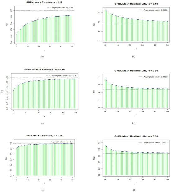
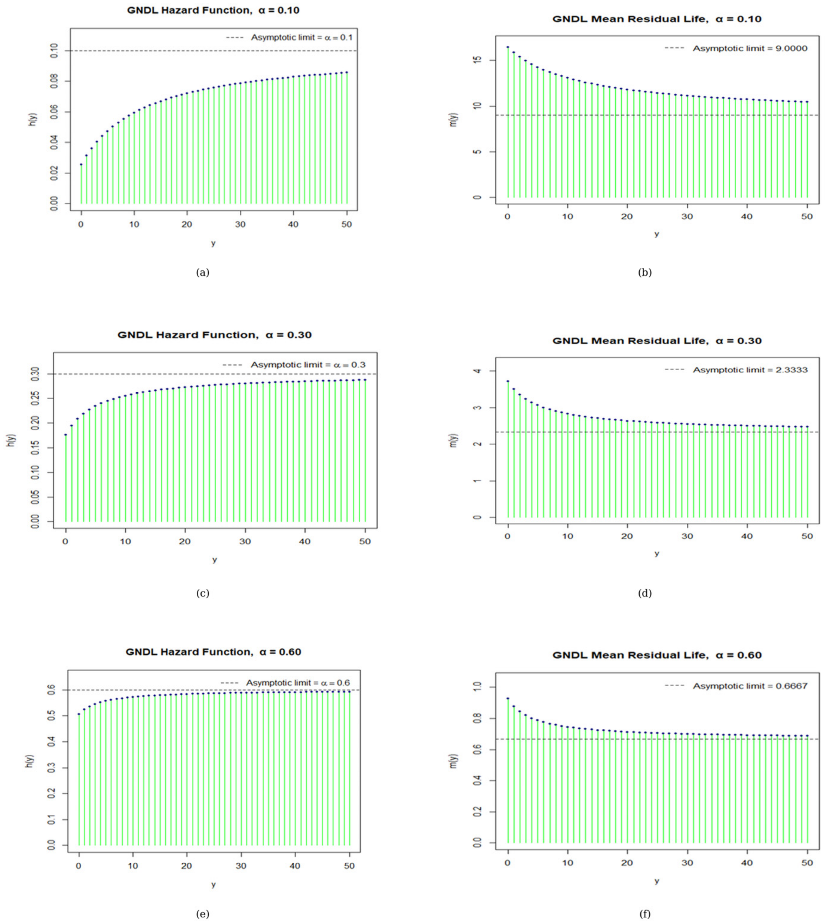
Figure 2 illustrates the increasing hazard-rate and decreasing mean-residual-life patterns for selected values of $\alpha$. The plots are consistent with, but are not used to establish, the analytical results in Theorem 5.

Figure 2. Hazard function (left column) and mean residual life function (right column) of the GNDL distribution: (a,b) $\alpha$ = 0.10; (c,d) $\alpha$ = 0.30; (e,f) $\alpha$= 0.60.

5.4. Aging Properties and Practical Stabilization Ages

Corollary 3.

For every  $0<\alpha <1$, the GNDL distribution belongs to the increasing-failure-rate (IFR) and decreasing-mean-residual-life (DMRL) classes. Under the discrete aging definitions and implication relationships discussed by Kemp [12],

$$\mathrm{I}\mathrm{F}\mathrm{R}\Rightarrow \mathrm{I}\mathrm{F}\mathrm{R}\mathrm{A}\Rightarrow \mathrm{N}\mathrm{B}\mathrm{U}\Rightarrow \mathrm{N}\mathrm{B}\mathrm{U}\mathrm{E}.$$

and

$$\mathrm{I}\mathrm{F}\mathrm{R}\Rightarrow \mathrm{D}\mathrm{M}\mathrm{R}\mathrm{L}\Rightarrow \mathrm{N}\mathrm{B}\mathrm{U}\mathrm{E}.$$

Consequently, the GNDL distribution also belongs to the IFRA, NBU, and NBUE classes [12,13].

Proof. 

The IFR and DMRL properties follow directly from the strict monotonicity results established in Theorem 5. Under the discrete aging definitions adopted by Kemp [12], the implication relationships above yield the IFRA, NBU, and NBUE properties. This completes the proof. □

Remark 3.

For fixed tolerances  ${\delta }_h>0$ and  ${\delta }_m>0$, define the practical stabilization ages

$$y_h^{*}\left(\alpha ,{\delta }_h\right)=\mathrm{m}\mathrm{i}\mathrm{n}\left\{y\in {\mathbb{N}}_0:\left|h\left(y;\alpha \right)-\alpha \right|\le {\delta }_h\right\},$$

and

$$y_m^{*}\left(\alpha ,{\delta }_m\right)=\mathrm{m}\mathrm{i}\mathrm{n}\left\{y\in {\mathbb{N}}_0:\left|m\left(y;\alpha \right)-{\displaystyle \frac{1-\alpha }{\alpha }}\right|\le {\delta }_m\right\}.$$

These minima are finite for every positive pair of tolerances, by the limiting results in Theorem 5.

Since

$$\left|h\left(y;\alpha \right)-\alpha \right|={\displaystyle \frac{\alpha \left(1-\alpha \right)}{{\left(1+\alpha \right)}^2+\alpha y}}$$

and

$$\left|m\left(y;\alpha \right)-{\displaystyle \frac{1-\alpha }{\alpha }}\right|={\displaystyle \frac{1-\alpha }{\alpha \left[{\left(1+\alpha \right)}^2+\alpha y\right]}},$$

the two thresholds are

$$y_h^{*}\left(\alpha ,{\delta }_h\right)=\mathrm{m}\mathrm{a}\mathrm{x}\left\{0,⌈{\displaystyle \frac{1-\alpha }{{\delta }_h}}-{\displaystyle \frac{{\left(1+\alpha \right)}^2}{\alpha }}⌉\right\},$$

and

$$y_m^{*}\left(\alpha ,{\delta }_m\right)=\mathrm{m}\mathrm{a}\mathrm{x}\left\{0,⌈{\displaystyle \frac{1-\alpha }{{\alpha }^2{\delta }_m}}-{\displaystyle \frac{{\left(1+\alpha \right)}^2}{\alpha }}⌉\right\}.$$

These quantities are the smallest integer ages at which the hazard rate and mean residual life, respectively, lie within the specified tolerances of their limiting values. They can be used as descriptive stabilization summaries, but they do not by themselves determine maintenance, warranty, or replacement decisions.

6. Stochastic Comparisons

Stochastic ordering provides a rigorous framework for comparing probability distributions in terms of their relative location, concentration, and tail behavior. This section establishes a likelihood-ratio ordering within the GNDL family as the parameter $\alpha$ varies. The resulting order implies the hazard-rate order, the usual stochastic order, and the increasing-convex order [13]. Thus, larger values of $\alpha$ correspond to stochastically smaller GNDL random variables.

Definition 2.

Let  $X$ and $Y$ be discrete random variables with probability mass functions $f$ and $g$, respectively, on a common ordered support $\mathcal{S}$, where $f\left(y\right)>0$ and $g\left(y\right)>0$ for every $y\in \mathcal{S}$. If $g\left(y\right)/f\left(y\right)$ is nondecreasing in $y\in \mathcal{S}$, then $X$ is said to be smaller than $Y$ in the likelihood-ratio order, denoted by $X{\le }_{lr}Y$.

Theorem 6.

Let  $Y_i$ follow the GNDL distribution with parameter  ${\alpha }_i$,$i=1,2$, where  $0<{\alpha }_1<{\alpha }_2<1$. Then

$$Y_2{\le }_{\mathrm{l}\mathrm{r}}{Y}_1.$$

Proof. 

Let $p_i\left(y\right)=p\left(y;{\alpha }_i\right)$, $i=1,2$, and define $L\left(y\right)=p_1\left(y\right)/p_2\left(y\right)$ for $y\in {\mathbb{N}}_0$. From the GNDL probability mass function in Equation (1),

$$L\left(y\right)=C{\left({\displaystyle \frac{1-{\alpha }_1}{1-{\alpha }_2}}\right)}^y\left[{\displaystyle \frac{3+{\alpha }_1+y}{3+{\alpha }_2+y}}\right], C={\displaystyle \frac{{\alpha }_1^2{\left(1+{\alpha }_2\right)}^2}{{\alpha }_2^2{\left(1+{\alpha }_1\right)}^2}}>0.$$

For every $y\in {\mathbb{N}}_0$,

$${\displaystyle \frac{L\left(y+1\right)}{L\left(y\right)}}={\displaystyle \frac{\left(1-{\alpha }_1\right)\left(4+{\alpha }_1+y\right)\left(3+{\alpha }_2+y\right)}{\left(1-{\alpha }_2\right)\left(3+{\alpha }_1+y\right)\left(4+{\alpha }_2+y\right)}}.$$

Since $0<{\alpha }_1<{\alpha }_2<1$,

$${\displaystyle \frac{1-{\alpha }_1}{1-{\alpha }_2}}>1.$$

Moreover,

$$\left(4+{\alpha }_1+y\right)\left(3+{\alpha }_2+y\right)-\left(3+{\alpha }_1+y\right)\left(4+{\alpha }_2+y\right)={\alpha }_2-{\alpha }_1>0,$$

and hence

$${\displaystyle \frac{\left(4+{\alpha }_1+y\right)\left(3+{\alpha }_2+y\right)}{\left(3+{\alpha }_1+y\right)\left(4+{\alpha }_2+y\right)}}>1.$$

Therefore,

$${\displaystyle \frac{L\left(y+1\right)}{L\left(y\right)}}>1, y\in {\mathbb{N}}_0.$$

Thus, $L\left(y\right)$ is strictly increasing in $y$, and Definition 2 yields $Y_2{\le }_{\mathrm{l}\mathrm{r}}{Y}_1$. This completes the proof. □

Corollary 4.

Under the assumptions of Theorem 6,

$$Y_2{\le }_{\mathrm{l}\mathrm{r}}{Y}_1\hspace{0.33em}\Rightarrow \hspace{0.33em}{Y}_2{\le }_{\mathrm{h}\mathrm{r}}{Y}_1\hspace{0.33em}\Rightarrow \hspace{0.33em}{Y}_2{\le }_{\mathrm{s}\mathrm{t}}{Y}_1\hspace{0.33em}\Rightarrow \hspace{0.33em}{Y}_2{\le }_{\mathrm{i}\mathrm{c}\mathrm{x}}{Y}_1.$$

Proof. 

The result follows from the standard implication relationships among the likelihood-ratio, hazard-rate, usual stochastic, and increasing-convex orders [13]. This completes the proof. □

Remark 4.

Theorem 6 shows that the GNDL family is stochastically decreasing in  $\alpha$. Consequently, for every  $y\in {\mathbb{N}}_0$,

$$F\left(y;{\alpha }_1\right)\le F\left(y;{\alpha }_2\right), S\left(y;{\alpha }_1\right)\ge S\left(y;{\alpha }_2\right),$$

and

$$\mathrm{E}\left(Y_2\right)\le \mathrm{E}\left(Y_1\right).$$

If

$$Q_{\alpha }\left(u\right)=\mathrm{i}\mathrm{n}\mathrm{f}\left\{y\in {\mathbb{N}}_0:F\left(y;\alpha \right)\ge u\right\}, 0<u<1,$$

then

$$Q_{{\alpha }_2}\left(u\right)\le Q_{{\alpha }_1}\left(u\right), 0<u<1.$$

7. Estimation Methods and Simulation Study

In this section, we consider estimation of the unknown parameter of the GNDL distribution using four frequentist methods: maximum likelihood estimation (MLE), the method of moments (MOM), the method of proportions (PE), and minimum chi-square estimation (MCS).

7.1. Maximum Likelihood Estimation (MLE)

Let $Y_1,Y_2,\dots ,Y_n$ be an independent and identically distributed random sample from the GNDL distribution, and let $y_1,y_2,\dots ,y_n$ denote the observed values. Based on the GNDL probability mass function, the log-likelihood function is

$$\mathcal{l}\left(\alpha \right)=2n\{\mathrm{l}\mathrm{o}\mathrm{g}\alpha -\mathrm{l}\mathrm{o}\mathrm{g}\left(1+\alpha \right)\}+\mathrm{l}\mathrm{o}\mathrm{g}\left(1-\alpha \right){\displaystyle \sum _{i=1}^n}{y}_i+{\displaystyle \sum _{i=1}^n}\mathrm{l}\mathrm{o}\mathrm{g}\left(3+\alpha +y_i\right), 0<\alpha <1.$$

(6)

Differentiating with respect to $\alpha$ gives the score function

$$U\left(\alpha \right)={\displaystyle \frac{\partial \mathcal{l}\left(\alpha \right)}{\partial \alpha }}={\displaystyle \frac{2n}{\alpha \left(1+\alpha \right)}}-{\displaystyle \frac{{\sum }_{i=1}^n{y}_i}{1-\alpha }}+{\displaystyle \sum _{i=1}^n}{\displaystyle \frac{1}{3+\alpha +y_i}}.$$

The second derivative is

$${\mathcal{l}}^{″}\left(\alpha \right)=-{\displaystyle \frac{2n\left(1+2\alpha \right)}{{\alpha }^2{\left(1+\alpha \right)}^2}}-{\displaystyle \frac{{\sum }_{i=1}^n{y}_i}{{\left(1-\alpha \right)}^2}}-{\displaystyle \sum _{i=1}^n}{\displaystyle \frac{1}{{\left(3+\alpha +y_i\right)}^2}}<0, 0<\alpha <1.$$

Thus, the log-likelihood is strictly concave. If the sample contains at least one positive observation, then ${\sum }_{i=1}^n{y}_i>0$, $U\left(\alpha \right)\to +\mathrm{\infty }$ as $\alpha \downarrow 0$, and $U\left(\alpha \right)\to -\mathrm{\infty }$ as $\alpha \uparrow 1$. Consequently, the score equation $U\left(\alpha \right)=0$ has a unique solution, denoted by ${\widehat{\alpha }}_{\mathrm{M}\mathrm{L}\mathrm{E}}$. This solution is obtained numerically by a one-dimensional root-finding procedure. If all observations are zero, then $U\left(\alpha \right)>0$ for every $0<\alpha <1$; hence, no MLE exists in the open parameter space, and the likelihood approaches its supremum as $\alpha \uparrow 1$.

For large-sample inference, the observed information obtained from the preceding second derivative is

$$J_n\left(\alpha \right)=-{\mathcal{l}}^{″}\left(\alpha \right)={\displaystyle \frac{2n\left(1+2\alpha \right)}{{\alpha }^2{\left(1+\alpha \right)}^2}}+{\displaystyle \sum _{i=1}^n}{\displaystyle \frac{y_i}{{\left(1-\alpha \right)}^2}}+{\displaystyle \sum _{i=1}^n}{\displaystyle \frac{1}{{\left(3+\alpha +y_i\right)}^2}}.$$

Taking expectation under the model gives the Fisher information per observation in the exact form

$$I_1\left(\alpha \right)={\displaystyle \frac{2\left(1+2\alpha \right)}{{\alpha }^2{\left(1+\alpha \right)}^2}}+{\displaystyle \frac{{\alpha }^2+2\alpha +2}{\alpha {\left(1+\alpha \right)}^2\left(1-\alpha \right)}}+{\displaystyle \frac{{\alpha }^2}{{\left(1+\alpha \right)}^2}}\Phi \left(1-\alpha ,1,3+\alpha \right).$$

Here, $\Phi$ denotes the Hurwitz–Lerch transcendent already used in Section 4.1. The final term follows directly by substituting the probability mass function into the expectation. Every term in the information is finite and strictly positive at each interior parameter value. For a sample of size $n$, independence gives

$$I_n\left(\alpha \right)=n{I}_1\left(\alpha \right).$$

The model is identifiable because $p_0\left(\alpha \right)={\alpha }^2\left(3+\alpha \right)/{\left(1+\alpha \right)}^2$ is strictly increasing on $\left(0,1\right)$. Since the support is parameter-independent and the probability mass function is positive and twice continuously differentiable on compact subsets of the interior, the standard likelihood regularity conditions for i.i.d. samples apply at any fixed interior true value ${\alpha }_0$. In particular,

$${\widehat{\alpha }}_{\mathrm{M}\mathrm{L}\mathrm{E}}\stackrel{p}{\to }{\alpha }_0,$$

Moreover,

$$\sqrt{n}\left({\widehat{\alpha }}_{\mathrm{M}\mathrm{L}\mathrm{E}}-{\alpha }_0\right)\stackrel{d}{\to }N\left(0,I_1{\left({\alpha }_0\right)}^{-1}\right).$$

The exceptional all-zero sample does not alter these asymptotic conclusions, because for every fixed ${\alpha }_0\in \left(0,1\right)$,

$$\underset{{\alpha }_0}{\mathrm{P}\mathrm{r}}\left(Y_1=\cdots =Y_n=0\right)={\left[{\displaystyle \frac{{\alpha }_0^2\left(3+{\alpha }_0\right)}{{\left(1+{\alpha }_0\right)}^2}}\right]}^n\to 0.$$

Thus an asymptotic standard error can be estimated by

$$\widehat{SE}\left({\widehat{\alpha }}_{\mathrm{M}\mathrm{L}\mathrm{E}}\right)={\left[n{I}_1\left({\widehat{\alpha }}_{\mathrm{M}\mathrm{L}\mathrm{E}}\right)\right]}^{-1/2}.$$

A two-sided $100\left(1-\gamma \right)\%$ Wald confidence interval is

$${\widehat{\alpha }}_{\mathrm{M}\mathrm{L}\mathrm{E}}\pm z_{1-\gamma /2}\widehat{SE}\left({\widehat{\alpha }}_{\mathrm{M}\mathrm{L}\mathrm{E}}\right).$$

For estimates close to the parameter-space boundaries, a logit-scale Wald interval can be used. Define

$$\widehat{\eta }=\mathrm{l}\mathrm{o}\mathrm{g}\left({\displaystyle \frac{{\widehat{\alpha }}_{\mathrm{M}\mathrm{L}\mathrm{E}}}{1-{\widehat{\alpha }}_{\mathrm{M}\mathrm{L}\mathrm{E}}}}\right), \widehat{SE}\left(\widehat{\eta }\right)={\displaystyle \frac{\widehat{SE}\left({\widehat{\alpha }}_{\mathrm{M}\mathrm{L}\mathrm{E}}\right)}{{\widehat{\alpha }}_{\mathrm{M}\mathrm{L}\mathrm{E}}\left(1-{\widehat{\alpha }}_{\mathrm{M}\mathrm{L}\mathrm{E}}\right)}}.$$

The corresponding interval on the original parameter scale is

$$\left[\mathrm{e}\mathrm{x}\mathrm{p}\mathrm{i}\mathrm{t}\left(\widehat{\eta }-z_{1-\gamma /2}\widehat{SE}\left(\widehat{\eta }\right)\right),\hspace{0.33em}\mathrm{e}\mathrm{x}\mathrm{p}\mathrm{i}\mathrm{t}\left(\widehat{\eta }+z_{1-\gamma /2}\widehat{SE}\left(\widehat{\eta }\right)\right)\right],$$

where $\mathrm{e}\mathrm{x}\mathrm{p}\mathrm{i}\mathrm{t}\left(u\right)=e^u/\left(1+e^u\right)$. This transformed interval remains inside the admissible parameter space $\left(0,1\right)$.

7.2. Method of Moments (MOM)

The MOM estimator is obtained by equating the observed sample mean $\overline{y}=n^{-1}{\sum }_{i=1}^n{y}_i$ to the theoretical mean of the GNDL distribution:

$$\overline{y}=\mu \left(\alpha \right)={\displaystyle \frac{\left(1-\alpha \right)\left({\alpha }^2+2\alpha +2\right)}{\alpha {\left(1+\alpha \right)}^2}}.$$

The theoretical mean is strictly decreasing in $\alpha$, because

$${\mu }^{\prime }\left(\alpha \right)=-{\displaystyle \frac{{\alpha }^3+{\alpha }^2+6\alpha +2}{{\alpha }^2{\left(1+\alpha \right)}^3}}<0, 0<\alpha <1.$$

Moreover, $\mu \left(\alpha \right)\to +\mathrm{\infty }$ as $\alpha \downarrow 0$ and $\mu \left(\alpha \right)\to 0$ as $\alpha \uparrow 1$. Therefore, every positive sample mean yields a unique solution ${\widehat{\alpha }}_{\mathrm{M}\mathrm{O}\mathrm{M}}\in \left(0,1\right)$, which is obtained numerically from the moment equation. For an all-zero sample, the equation is satisfied only in the limiting sense as $\alpha \uparrow 1$.

7.3. Method of Proportions (PE)

The method of proportions estimates unknown parameters of a discrete distribution by equating an observed sample proportion to the corresponding probability under the model [14,15]. Let

$$N_0={\displaystyle \sum _{i=1}^n}I\left(y_i=0\right), {\widehat{p}}_0={\displaystyle \frac{N_0}{n}},$$

where $I\left(\cdot \right)$ is the indicator function. For the GNDL distribution,

$$p_0\left(\alpha \right)=P_{\alpha }\left(Y=0\right)={\displaystyle \frac{{\alpha }^2\left(3+\alpha \right)}{{\left(1+\alpha \right)}^2}}.$$

Accordingly, the proportion estimator ${\widehat{\alpha }}_{\mathrm{P}\mathrm{E}}$ is defined as the solution of

$${\widehat{p}}_0={\displaystyle \frac{{\alpha }^2\left(3+\alpha \right)}{{\left(1+\alpha \right)}^2}}, 0<\alpha <1.$$

The probability $p_0\left(\alpha \right)$ is strictly increasing, since

$${p_0}^{\prime }\left(\alpha \right)={\displaystyle \frac{\alpha \left({\alpha }^2+3\alpha +6\right)}{{\left(1+\alpha \right)}^3}}>0, 0<\alpha <1.$$

Because $p_0\left(\alpha \right)\to 0$ as $\alpha \downarrow 0$ and $p_0\left(\alpha \right)\to 1$ as $\alpha \uparrow 1$, the estimating equation has a unique solution in $\left(0,1\right)$ whenever $0<{\widehat{p}}_0<1$. If ${\widehat{p}}_0=0$, the solution exists only in the limiting sense as $\alpha \downarrow 0$; if ${\widehat{p}}_0=1$, it exists only in the limiting sense as $\alpha \uparrow 1$.

7.4. Minimum Chi-Square Estimation

The minimum chi-square method estimates the model parameter by minimizing the discrepancy between the empirical and theoretical probability masses [16]. Let $Y_1,Y_2,\dots ,Y_n$ be a random sample from the GNDL distribution, and define

$$Y_{\left(n\right)}=\mathrm{m}\mathrm{a}\mathrm{x}\{Y_1,Y_2,\dots ,Y_n\}.$$

For $k=0,1,\dots ,Y_{\left(n\right)}$, the empirical relative frequency of the value $k$ is

$${\widehat{p}}_k={\displaystyle \frac{1}{n}}{\displaystyle \sum _{i=1}^n}I\left(Y_i=k\right),$$

where $I\left(\cdot \right)$ denotes the indicator function. The corresponding GNDL probability mass is

$$p_k\left(\alpha \right)=P\left(Y=k;\alpha \right)={\displaystyle \frac{{\alpha }^2\left(3+\alpha +k\right){\left(1-\alpha \right)}^k}{{\left(1+\alpha \right)}^2}}, k=0,1,2,\dots , 0<\alpha <1.$$

The minimum chi-square discrepancy is defined as

$${\chi }^2\left(\alpha \right)={\displaystyle \sum _{k=0}^{\mathrm{\infty }}}{\displaystyle \frac{{\left[{\widehat{p}}_k-p_k\left(\alpha \right)\right]}^2}{p_k\left(\alpha \right)}}.$$

The criterion above is the normalized Pearson chi-square discrepancy. Multiplication by n gives the usual Pearson form and does not alter the minimizing value of α.

Since ${\widehat{p}}_k=0$ for every $k>Y_{\left(n\right)}$, the infinite sum can be written equivalently as

$${\chi }^2\left(\alpha \right)={\displaystyle \sum _{k=0}^{Y_{\left(n\right)}}}{\displaystyle \frac{{\left[{\widehat{p}}_k-p_k\left(\alpha \right)\right]}^2}{p_k\left(\alpha \right)}}+\left[1-F\left(Y_{\left(n\right)};\alpha \right)\right].$$

For the GNDL distribution, the right-tail probability is

$$1-F\left(Y_{\left(n\right)};\alpha \right)={\displaystyle \frac{\left(1+3\alpha +{\alpha }^2+\alpha Y_{\left(n\right)}\right){\left(1-\alpha \right)}^{Y_{\left(n\right)}+1}}{{\left(1+\alpha \right)}^2}}.$$

The minimum chi-square estimator of $\alpha$ is therefore defined by

$${\widehat{\alpha }}_{\mathrm{M}\mathrm{C}\mathrm{S}}=\underset{0<\alpha <1}{\mathrm{a}\mathrm{r}\mathrm{g} \mathrm{m}\mathrm{i}\mathrm{n}}\hspace{0.33em}{\chi }^2\left(\alpha \right).$$

Because a closed-form solution is generally unavailable, ${\widehat{\alpha }}_{\mathrm{M}\mathrm{C}\mathrm{S}}$ is obtained numerically. In the numerical implementation, minimization is carried out over ${10}^{-8}\le \alpha \le 1-{10}^{-8}$, and any solution attained at an endpoint is retained and reported as a boundary estimate.

7.5. Monte Carlo Simulation Study

A Monte Carlo simulation study was conducted to examine the finite-sample performance of the maximum likelihood estimator (MLE), the method-of-moments estimator (MOM), the method of proportions (PE), and the minimum chi-square estimator (MCS) for the GNDL parameter α. The design covers parameter values producing count patterns from highly dispersed to strongly concentrated and sample sizes ranging from small to large, thereby permitting a systematic assessment of estimator centering, sampling variability, boundary behavior, and overall accuracy.

The simulation design was specified as follows.

• The parameter values were $\alpha \in \{0.1,0.3,0.5,0.7,0.9\}$
• The sample sizes were $n\in \{20,30,50,100,150,300\}$, producing 30 parameter-sample-size configurations.
• For each configuration, $R = 5000$ independent Monte Carlo replications were performed. A fixed master seed of 12,345 and setup-specific derived seeds were used to make every configuration reproducible. In replication $r,$ the sample $Y_{\mathrm{r}} = (Y_{\mathrm{r}1}, \dots , Y_{\mathrm{r}\mathrm{n}})$ was generated independently from the GNDL distribution.
• Each observation was generated exactly through the equivalent geometric–negative binomial stochastic representation. First, an indicator Z_ri was generated with success probability ${(1 + \alpha )}^{-2}.$ Conditional on this indicator, the observation was generated from either a geometric component or a negative binomial component with size parameter 2, as follows.

$$Z_{ri}\sim \mathrm{B}\mathrm{e}\mathrm{r}\mathrm{n}\mathrm{o}\mathrm{u}\mathrm{l}\mathrm{l}\mathrm{i}\left({\displaystyle \frac{1}{{\left(1+\alpha \right)}^2}}\right), i=1,\dots ,n, r=1,\dots ,R,$$

$$Y_{ri}\mid Z_{ri}=0\sim \mathrm{G}\mathrm{e}\mathrm{o}\mathrm{m}\mathrm{e}\mathrm{t}\mathrm{r}\mathrm{i}\mathrm{c}\left(\alpha \right), Y_{ri}\mid Z_{ri}=1\sim \mathrm{N}\mathrm{e}\mathrm{g}\mathrm{a}\mathrm{t}\mathrm{i}\mathrm{v}\mathrm{e} \mathrm{B}\mathrm{i}\mathrm{n}\mathrm{o}\mathrm{m}\mathrm{i}\mathrm{a}\mathrm{l}\left(2,\alpha \right),$$

$$P\left(Y_{ri}=y\mid Z_{ri}=0\right)=\alpha {\left(1-\alpha \right)}^y, P\left(Y_{ri}=y\mid Z_{ri}=1\right)=\left(y+1\right){\alpha }^2{\left(1-\alpha \right)}^y, y\in {\mathbb{N}}_0.$$

The resulting marginal probability mass function is

$$P\left(Y_{ri}=y\right)={\displaystyle \frac{{\alpha }^2\left(3+\alpha +y\right){\left(1-\alpha \right)}^y}{{\left(1+\alpha \right)}^2}}, y\in {\mathbb{N}}_0,$$

which is the GNDL probability mass function. Hence, the simulation procedure generates observations exactly from the proposed distribution and does not require numerical inversion or truncation of the support.

5.

Within each replication, the same generated sample was used to compute MLE, MOM, PE, and MCS, ensuring paired comparisons under identical sampling variation. MLE, MOM, and every interior PE estimate were obtained by solving their unique one-dimensional estimating equations with numerical tolerance ${10}^{-10}.$ For MCS, empirical frequencies were formed on $\{0,\dots ,Y_{r,\left(n\right)}\}$, where $Y_{r,\left(n\right)}=\max \{Y_{r1},\dots ,Y_{rn}\}$ is the sample maximum in replication $r$, and the exact unobserved right-tail probability beyond $Y_{r,\left(n\right)}$ was included. The MCS objective was minimized by a safeguarded global one-dimensional search: an 81-point regular grid augmented by points near both boundaries was used to identify candidate basins, each candidate basin was refined by Brent minimization, and both endpoints were checked explicitly.

6.

The theoretical parameter space $0 < \alpha < 1$ was implemented numerically as $\epsilon \le \alpha \le 1 - \epsilon ,$ where $\epsilon = {10}^{-8},$ to avoid evaluation at the degenerate endpoints. Estimates equal to either bound were classified as boundary estimates and retained in every Monte Carlo summary rather than treated as optimization failures. An all-zero sample yields the upper-bound estimate $1 - \epsilon$ for all four procedures. For PE, a sample containing no zero observations yields the lower-bound estimate $\epsilon$. Any MCS minimum attained at an endpoint was likewise retained and reported.

Let ${\widehat{\alpha }}_r$ denote the estimate obtained from replication $r$, where $r=1,2,\dots ,R$. The finite-sample performance of each estimator was summarized by the mean estimate, bias, root mean squared error (RMSE), and mean absolute error (MAE), defined respectively as

$$\overline{\widehat{\alpha }}={\displaystyle \frac{1}{R}}{\displaystyle \sum _{r=1}^R}{\widehat{\alpha }}_r,$$

$$\mathrm{B}\mathrm{i}\mathrm{a}\mathrm{s}\left(\widehat{\alpha }\right)={\displaystyle \frac{1}{R}}{\displaystyle \sum _{r=1}^R}\left({\widehat{\alpha }}_r-\alpha \right),$$

$$\mathrm{R}\mathrm{M}\mathrm{S}\mathrm{E}\left(\widehat{\alpha }\right)={\left[{\displaystyle \frac{1}{R}}{\displaystyle \sum _{r=1}^R}{\left({\widehat{\alpha }}_r-\alpha \right)}^2\right]}^{1/2},$$

$$\mathrm{M}\mathrm{A}\mathrm{E}\left(\widehat{\alpha }\right)={\displaystyle \frac{1}{R}}{\displaystyle \sum _{r=1}^R}\left|{\widehat{\alpha }}_r-\alpha \right|.$$

The mean estimate describes the centering of the sampling distribution, while bias quantifies systematic deviation from the true parameter value. RMSE combines squared bias and sampling variability, whereas MAE measures the average absolute estimation error. Table 1, Table 2, Table 3 and Table 4 report these measures for MLE, MOM, PE, and MCS, respectively. Observed boundary-solution rates are reported in Table 5, while success rates and additional numerical diagnostics were retained in the simulation output for quality-control purposes.

Table 1. Simulation results for the maximum likelihood estimator of $\alpha$.

$\mathit{\alpha }$	$\mathit{n}$	Mean	Bias	RMSE	MAE
0.1	20	0.102316	0.002316	0.016093	0.012508
	30	0.101570	0.001570	0.012641	0.009838
	50	0.100967	0.000967	0.009860	0.007749
	100	0.100443	0.000443	0.006818	0.005388
	150	0.100304	0.000304	0.005651	0.004500
	300	0.100086	0.000086	0.003952	0.003132
0.3	20	0.306273	0.006273	0.044389	0.034623
	30	0.304188	0.004188	0.034919	0.027408
	50	0.302554	0.002554	0.026971	0.021319
	100	0.301248	0.001248	0.018853	0.014850
	150	0.301041	0.001041	0.015457	0.012310
	300	0.300365	0.000365	0.010681	0.008502
0.5	20	0.507468	0.007468	0.063231	0.049967
	30	0.505647	0.005647	0.051855	0.041063
	50	0.503615	0.003615	0.039383	0.031353
	100	0.501989	0.001989	0.028156	0.022471
	150	0.500807	0.000807	0.022594	0.017998
	300	0.500475	0.000475	0.016035	0.012804
0.7	20	0.707117	0.007117	0.070845	0.056537
	30	0.705164	0.005164	0.059307	0.047647
	50	0.704865	0.004865	0.045382	0.036150
	100	0.700933	0.000933	0.031718	0.025338
	150	0.701196	0.001196	0.025960	0.020712
	300	0.700652	0.000652	0.018328	0.014714
0.9	20	0.905250	0.005250	0.054261	0.043771
	30	0.902364	0.002364	0.044385	0.035965
	50	0.901999	0.001999	0.034918	0.027949
	100	0.900803	0.000803	0.024594	0.019736
	150	0.900571	0.000571	0.020386	0.016322
	300	0.900422	0.000422	0.014328	0.011493

Table 2. Simulation results for the method-of-moments estimator of $\alpha$.

$\mathit{\alpha }$	$\mathit{n}$	Mean	Bias	RMSE	MAE
0.1	20	0.102323	0.002323	0.016096	0.012510
	30	0.101574	0.001574	0.012643	0.009839
	50	0.100970	0.000970	0.009862	0.007750
	100	0.100444	0.000444	0.006819	0.005388
	150	0.100305	0.000305	0.005651	0.004501
	300	0.100087	0.000087	0.003952	0.003132
0.3	20	0.306315	0.006315	0.044402	0.034631
	30	0.304222	0.004222	0.034926	0.027411
	50	0.302576	0.002576	0.026978	0.021325
	100	0.301257	0.001257	0.018855	0.014853
	150	0.301048	0.001048	0.015458	0.012311
	300	0.300368	0.000368	0.010682	0.008501
0.5	20	0.507533	0.007533	0.063239	0.049966
	30	0.505689	0.005689	0.051852	0.041063
	50	0.503635	0.003635	0.039383	0.031354
	100	0.502000	0.002000	0.028154	0.022471
	150	0.500816	0.000816	0.022596	0.018000
	300	0.500479	0.000479	0.016034	0.012803
0.7	20	0.707160	0.007160	0.070836	0.056532
	30	0.705189	0.005189	0.059303	0.047644
	50	0.704884	0.004884	0.045380	0.036145
	100	0.700941	0.000941	0.031717	0.025337
	150	0.701202	0.001202	0.025959	0.020711
	300	0.700656	0.000656	0.018327	0.014713
0.9	20	0.905259	0.005259	0.054254	0.043765
	30	0.902369	0.002369	0.044380	0.035962
	50	0.902002	0.002002	0.034916	0.027948
	100	0.900804	0.000804	0.024594	0.019736
	150	0.900573	0.000573	0.020385	0.016321
	300	0.900422	0.000422	0.014328	0.011493

Table 3. Simulation results for the method-of-proportions estimator of $\alpha$.

$\mathit{\alpha }$	$\mathit{n}$	Mean	Bias	RMSE	MAE
0.1	20	0.065966	−0.034034	0.089794	0.084926
	30	0.075080	−0.024920	0.076922	0.065600
	50	0.082469	−0.017531	0.061854	0.048894
	100	0.092797	−0.007203	0.039688	0.030559
	150	0.096670	−0.003330	0.029581	0.022868
	300	0.098383	−0.001617	0.019866	0.015765
0.3	20	0.293248	−0.006752	0.096470	0.076456
	30	0.294420	−0.005580	0.075476	0.060007
	50	0.296929	−0.003071	0.057097	0.045408
	100	0.298662	−0.001338	0.039913	0.031677
	150	0.299039	−0.000961	0.032731	0.026127
	300	0.299690	−0.000310	0.022972	0.018397
0.5	20	0.496189	−0.003811	0.095249	0.076226
	30	0.498608	−0.001392	0.080022	0.064316
	50	0.500254	0.000254	0.060549	0.048476
	100	0.500310	0.000310	0.042400	0.033685
	150	0.499608	−0.000392	0.034619	0.027693
	300	0.499872	−0.000128	0.024649	0.019663
0.7	20	0.697914	−0.002086	0.088260	0.070747
	30	0.700409	0.000409	0.073492	0.058348
	50	0.700776	0.000776	0.056011	0.045004
	100	0.699188	−0.000812	0.039364	0.031291
	150	0.699799	−0.000201	0.032329	0.025702
	300	0.699854	−0.000146	0.022829	0.018265
0.9	20	0.900902	0.000902	0.059607	0.048825
	30	0.899677	−0.000323	0.048505	0.038975
	50	0.900301	0.000301	0.037719	0.030218
	100	0.900092	0.000092	0.026238	0.021089
	150	0.899784	−0.000216	0.021956	0.017494
	300	0.900170	0.000170	0.015229	0.012252

Table 4. Simulation results for the minimum chi-square estimator of $\alpha$.

$\mathit{\alpha }$	$\mathit{n}$	Mean	Bias	RMSE	MAE
0.1	20	0.081680	−0.018320	0.023793	0.020568
	30	0.081340	−0.018660	0.022658	0.019854
	50	0.082126	−0.017874	0.020924	0.018443
	100	0.084135	−0.015865	0.017975	0.016056
	150	0.085645	−0.014355	0.016156	0.014442
	300	0.088555	−0.011445	0.012855	0.011485
0.3	20	0.262151	−0.037849	0.058917	0.049426
	30	0.264223	−0.035777	0.051516	0.043219
	50	0.268612	−0.031388	0.043892	0.036433
	100	0.274501	−0.025499	0.034673	0.028574
	150	0.278779	−0.021221	0.028962	0.023500
	300	0.284101	−0.015899	0.021887	0.017385
0.5	20	0.457791	−0.042209	0.080503	0.065917
	30	0.462816	−0.037184	0.067712	0.055527
	50	0.467417	−0.032583	0.055732	0.045027
	100	0.475322	−0.024678	0.041906	0.033269
	150	0.478711	−0.021289	0.035814	0.028061
	300	0.484760	−0.015240	0.025861	0.019900
0.7	20	0.666527	−0.033473	0.086729	0.069603
	30	0.670347	−0.029653	0.073726	0.058802
	50	0.676668	−0.023332	0.057347	0.045841
	100	0.680294	−0.019706	0.042577	0.033340
	150	0.684082	−0.015918	0.035136	0.027215
	300	0.688972	−0.011028	0.024961	0.019134
0.9	20	0.890078	−0.009922	0.065986	0.054573
	30	0.888039	−0.011961	0.054163	0.043026
	50	0.889903	−0.010097	0.042272	0.033057
	100	0.891734	−0.008266	0.029793	0.023402
	150	0.892968	−0.007032	0.024872	0.019075
	300	0.894982	−0.005018	0.017558	0.013472

Table 5. Observed nonzero boundary-solution rates (5000 replications).

$\mathit{\alpha }$	$\mathit{n}$	Estimator(s)	Boundary Rate	Reason for Boundary Estimate
0.1	20	PE	59.48%	No zero observations; lower boundary
0.1	30	PE	45.26%	No zero observations; lower boundary
0.1	50	PE	28.84%	No zero observations; lower boundary
0.1	100	PE	7.68%	No zero observations; lower boundary
0.1	150	PE	1.80%	No zero observations; lower boundary
0.1	300	PE	0.02%	No zero observations; lower boundary
0.3	20	PE	1.88%	No zero observations; lower boundary
0.3	30	PE	0.26%	No zero observations; lower boundary
0.9	20	MLE, MOM, PE, MCS	7.20%	All-zero sample; upper boundary
0.9	30	MLE, MOM, PE, MCS	1.52%	All-zero sample; upper boundary
0.9	50	MLE, MOM, PE, MCS	0.26%	All-zero sample; upper boundary

PE is based only on the empirical zero proportion ${\widehat{p}}_0=N_0/n$. For GNDL,

$$p_0\left(\alpha \right)=P_{\alpha }\left(Y=0\right)={\displaystyle \frac{{\alpha }^2\left(3+\alpha \right)}{{\left(1+\alpha \right)}^2}}$$

$${p_0}^{\prime }\left(\alpha \right)={\displaystyle \frac{\alpha \left({\alpha }^2+3\alpha +6\right)}{{\left(1+\alpha \right)}^3}}>0$$

A sample with no observed zeros forces the PE solution to the implemented lower boundary. The exact probability of this event is

$$P_{\alpha }\left(N_0=0\right)={\left[1-p_0\left(\alpha \right)\right]}^n$$

This explains the simulation pattern quantitatively. At $\alpha =0.1$, $p_0\left(\alpha \right)=P_{\alpha }\left(Y=0\right)={\displaystyle \frac{{\alpha }^2\left(3+\alpha \right)}{{\left(1+\alpha \right)}^2}}$ evaluates to 0.025620, so the probability of observing no zeros is approximately 0.5951 at n = 20, 0.2732 at n = 50, 0.0746 at n = 100, and 0.00042 at n = 300. In contrast, at $\alpha =0.3$, the no-zero probability is already only about 0.0210 at n = 20 and 0.000064 at n = 50. Thus PE is specifically vulnerable when α is small and n is small; its centering becomes competitive once zero counts are sufficiently represented in the sample.

Across the 30 reported configurations, MLE and MOM are numerically almost identical. At the reported precision, the maximum absolute RMSE difference is about $1.3\times {10}^{-5}$ and the maximum absolute MAE difference is about $8\times {10}^{-6}$, respectively. They are not algebraically identical estimators. The empirical closeness is consistent with the one-parameter structure: the theoretical mean is strictly monotone in $\alpha$, so the sample mean carries a strong one-dimensional signal, while the likelihood uses the full sample and adds only a modest refinement over that signal in the examined parameter region. We therefore describe this as an empirical finite-sample similarity, not as a theoretical identity.

MCS remains numerically stable and improves as n increases, but the simulations show persistent finite-sample underestimation. The Pearson-type criterion weights discrepancies by inverse fitted probabilities, so sparse and tail cells can exert relatively high leverage when samples are small. This provides a plausible finite-sample mechanism consistent with the observed negative bias; it is stated as an interpretation rather than a theorem. As n increases, empirical cell proportions stabilize, while RMSE decreases and the overall magnitude of the bias generally becomes smaller.

The simulation results reveal estimator-specific operating regimes rather than a universal winner. MLE and MOM provide the most consistently favorable precision over the full design, with nearly indistinguishable RMSE and MAE. PE is primarily a centering-oriented estimator: when the expected number of zeros is adequate, its bias can be very small, particularly for moderate and large α. Its weakness at small α and small n follows directly from its reliance on the zero proportion: if N₀ = 0, the estimate is forced to the lower boundary. For α = 0.1, this event has probabilities approximately 0.595, 0.273, 0.075, and 0.0004 at n = 20, 50, 100, and 300, respectively, explaining the pronounced negative bias and its rapid attenuation with n. MCS is stable and its RMSE decreases with n, but it retains a downward finite-sample bias, consistent with the greater influence of sparse cells in the Pearson-type discrepancy. Hence MLE/MOM are preferred when precision and stability are primary, PE can be attractive for centering once the zero cell is sufficiently sampled, and MCS becomes more competitive as sample information increases.

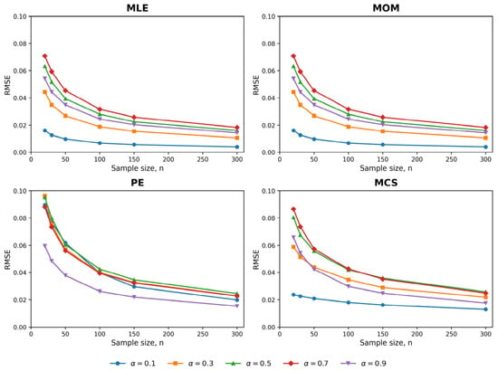
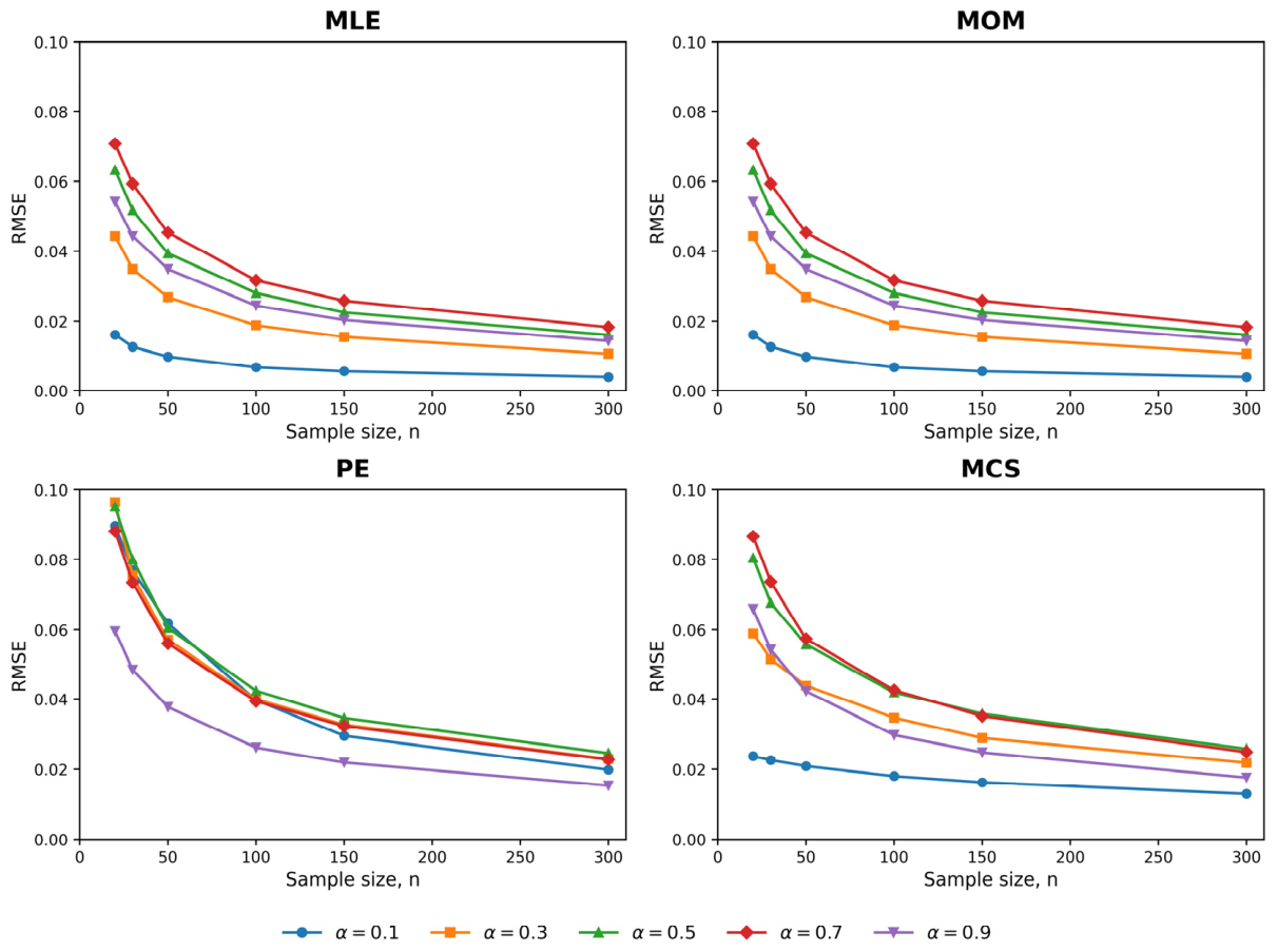
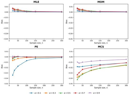
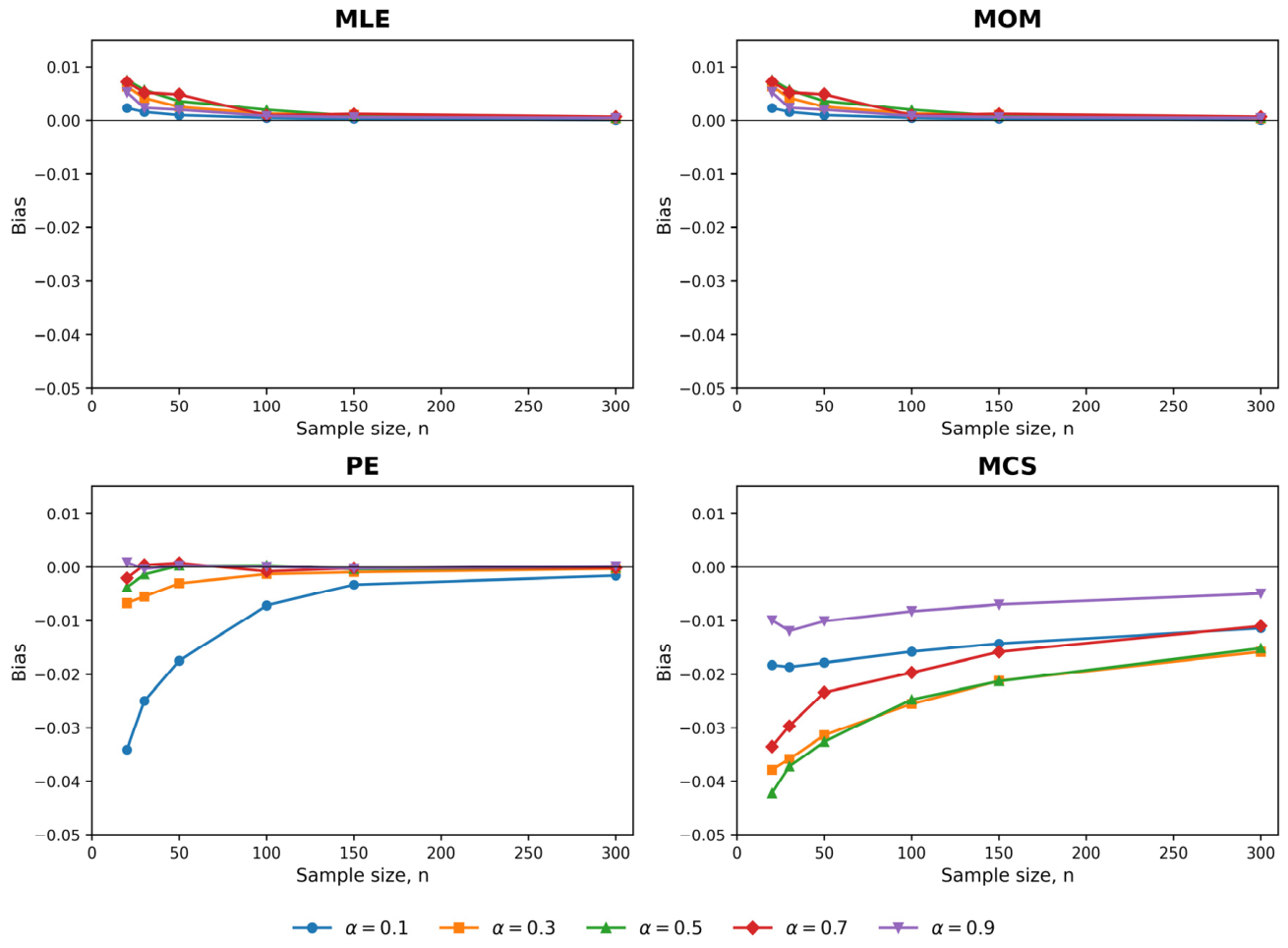
Figure 3 should be read as a precision comparison: all RMSE curves decline with n, but the near overlap of MLE and MOM shows that the additional likelihood information produces little finite-sample precision gain over the mean equation in the examined one-parameter model. Figure 4 separates the bias mechanisms: MLE and MOM show small positive bias that generally decreases as n increases; PE shows strong negative bias only in the low-$\alpha$ boundary-sensitive region and rapidly recenters as the probability of observing at least one zero approaches one; MCS remains negatively biased across the grid, although its bias magnitude generally decreases as n increases. Thus, the two figures jointly show a bias–precision trade-off, not merely convergence with sample size.

Figure 3. RMSE of the considered estimators MLE, MOM, PE, and MCS for the considered values of α.

Figure 4. Bias of the considered estimators MLE, MOM, PE, and MCS for the considered values of α.

All omitted configurations had 0% boundary rates. The numerical bounds were ${10}^{-8}$ and $1 - {10}^{-8}$. At small $\alpha$, PE boundary estimates came from no-zero samples (lower bound); at $\alpha = 0.9$, all four estimators’ boundary estimates came from all-zero samples (upper bound).

8. Applications to Real Data

This section examines the empirical performance and practical usefulness of the GNDL distribution using four real data sets from distinct application domains. Data set 1 contains grouped pulmonary-exacerbation counts for the treatment group of patients with cystic fibrosis over a 169-day follow-up period, as reported by Lawless [17]. Data set 2 comprises grouped automobile-insurance claim counts per policy reported by Gossiaux and Lemaire [18] and Puig and Valero [19]. Data set 3 consists of 123 observations on the numbers of fires in forest districts of Greece during 1 July–31 August 1998, as analyzed by Altun et al. [20]. Data set 4 contains remission times, measured in weeks, for 20 leukemia patients, as analyzed by Bakouch et al. [21].

Table 6 summarizes the empirical characteristics of the four data sets. The sample variance exceeds the sample mean in every case, while the strength and form of the dispersion differ markedly across the applications. The first two data sets are highly concentrated at zero, whereas the third count data set and the discrete lifetime data display substantially wider ranges and stronger overdispersion. These differences provide a heterogeneous setting for assessing the practical performance of the proposed model.

Table 6. Descriptive statistics for the four real data sets.

Data Set	$\mathit{n}$	Mean	Variance	Variance/Mean	Zero Proportion	Range
Data set 1	321	0.482866	0.662987	1.373024	0.676012	0–4
Data set 2	23,589	0.144220	0.163870	1.136252	0.872949	0–6
Data set 3	123	5.398374	30.044915	5.565549	0.130081	0–43
Data set 4	20	19.550000	216.050000	11.051151	0.000000	1–49

The GNDL distribution is compared with the classical and contemporary one- and two-parameter discrete models listed in Table 7. All fitted parameters are obtained by maximum likelihood over the implemented parameter spaces, with boundary solutions retained when they occur. All likelihood, goodness-of-fit, and information-criterion calculations use unrounded estimates; rounding is applied only to the reported presentation values. For the TNDL/2P-PLD row, the two reported estimates are the equivalent Geo–NB2 coordinates defined in Section 2.

Table 7. Competing models and references.

Model	Abbreviation	Reference
Two-parameter TNDL/Poisson–Lindley equivalent family	TNDL/2P-PLD	[4,6]
Geometric	Geo	Standard distribution
Natural Discrete Lindley	NDL	[4]
Binomial–Natural Discrete Lindley	BNDL	[5]
Discrete Lindley	DLi	[3]
Negative binomial	NB	Standard distribution
Discrete Weibull	DW	[22]
Poisson	Poi	Standard distribution

For data sets 1–3, goodness of fit is assessed using the Pearson chi-square test, while comparative model performance is evaluated using the Akaike information criterion (AIC) and the Bayesian information criterion (BIC). For data sets 1 and 2, adjacent upper-tail categories are pooled until every final expected frequency is at least five. For data set 3, the same upper-tail pooling rule is applied and adjacent lower-tail categories are additionally pooled whenever necessary; this lower-tail correction is required for the Poisson fit, whose expected frequencies at the beginning of the support are below five. Pooling is performed separately for each fitted model because the expected frequencies differ across models. If $C$ is the number of final pooled cells and $k$ is the number of estimated parameters, the reported degrees of freedom are $C - 1 - k$. For data set 1, the original unpooled frequencies are displayed in Table 8, whereas the corresponding Pearson statistics and p-values are reported in Table 9. The corresponding frequency and Pearson results for data sets 2 and 3 are presented in Table 10 and Table 11 and Table 12 and Table 13, respectively. Because pooling patterns and degrees of freedom may differ across models, Pearson statistics are interpreted primarily as model-specific adequacy checks; comparative ranking is based mainly on AIC and BIC.

Table 8. Observed and expected frequencies of the fitted models for data set 1.

y	Obs	GNDL	TNDL/2P-PLD	Geo	NDL	BNDL	DLi	NB	DW	Poi
0	217	214.78	214.63	216.47	212.61	212.43	210.52	215.23	215.08	198.06
1	65	72.43	72.60	70.49	75.13	75.41	77.88	72.03	72.20	95.64
2	30	23.33	23.36	22.95	23.60	23.60	23.71	23.11	23.13	23.09
3	6	7.29	7.27	7.47	6.95	6.90	6.58	7.31	7.29	3.72
4	3	2.23	2.21	2.43	1.96	1.94	1.73	2.29	2.28	0.45
≥5	0	0.95	0.93	1.18	0.74	0.72	0.58	1.04	1.02	0.05
Total	321	321	321	321	321	321	321	321	321	321

Table 9. Parameter estimates, goodness-of-fit statistics, and information criteria for data set 1.

Model	Estimate(s)	Chi-Square	p-Value	df	AIC	BIC
GNDL	0.734021	2.8941	0.235263	2	602.4946	606.2661
TNDL/2P-PLD	0.736552; 0.350005	2.9020	0.088471	1	604.4932	612.0360
Geo	0.674370	2.9836	0.224965	2	602.7508	606.5223
NDL	0.764413	3.2365	0.198243	2	602.7543	606.5258
BNDL	0.696378	3.3012	0.191930	2	602.8147	606.5861
DLi	0.214263	4.0000	0.135338	2	603.5297	607.3011
NB	0.693045; 1.090218	3.0095	0.082780	1	604.6845	612.2274
DW	0.329959; 1.023071	3.0107	0.082718	1	604.6654	612.2083
Poi	0.482866	16.6375	0.000045	1	619.8432	623.6147

Table 10. Observed and expected frequencies of the fitted models for data set 2.

y	Obs	GNDL	TNDL/2P-PLD	Geo	NDL	BNDL	DLi	NB	DW	Poi
0	20,592	20,599.47	20,599.82	20,615.79	20,573.64	20,573.43	20,544.79	20,596.76	20,597.35	20,420.94
1	2651	2625.74	2625.14	2598.46	2670.15	2670.55	2720.36	2631.03	2629.92	2945.10
2	297	320.75	320.91	327.51	308.04	307.91	292.41	318.37	318.79	212.37
3	41	38.05	38.12	41.28	33.32	33.27	28.55	37.81	37.90	10.21
4	7	4.42	4.44	5.20	3.46	3.45	2.64	4.45	4.45	0.37
5	0	0.51	0.51	0.66	0.35	0.35	0.24	0.52	0.52	0.01
≥6	1	0.06	0.06	0.09	0.04	0.04	0.02	0.07	0.07	0.00
Total	23,589	23,589	23,589	23,589	23,589	23,589	23,589	23,589	23,589	23,589

Table 11. Parameter estimates, goodness-of-fit statistics, and information criteria for data set 2.

Model	Estimate(s)	Chi-Square	p-Value	df	AIC	BIC
GNDL	0.898555	2.8279	0.243184	2	20,449.3452	20,457.4137
TNDL/2P-PLD	0.898286; 0.273680	4.0440	0.132388	2	20,451.3448	20,467.4819
Geo	0.873958	4.6384	0.200271	3	20,449.9970	20,458.0655
NDL	0.913477	4.3201	0.115317	2	20,451.4283	20,459.4968
BNDL	0.905420	4.3567	0.113230	2	20,451.4686	20,459.5371
DLi	0.074965	11.7458	0.002815	2	20,458.9064	20,466.9749
NB	0.885732; 1.117895	3.5997	0.165326	2	20,450.8405	20,466.9776
DW	0.126824; 1.016579	3.6564	0.160706	2	20,450.9157	20,467.0528
Poi	0.144220	203.8740	<0.000001	2	20,597.6863	20,605.7548

Table 12. Observed and expected frequencies of the fitted models for data set 3.

y	Obs	GNDL	TNDL/2P-PLD	Geo	NDL	BNDL	DLi	NB	DW	Poi
0	16	14.38	14.79	19.22	12.30	30.75	10.86	14.17	14.79	0.56
1	13	14.41	14.53	16.22	13.84	30.75	13.50	15.18	15.29	3.00
2	14	13.63	13.60	13.68	13.84	23.06	14.04	14.21	13.98	8.11
3	9	12.42	12.32	11.55	12.97	15.37	13.39	12.67	12.37	14.59
4	11	11.03	10.91	9.74	11.68	9.61	12.13	11.01	10.75	19.69
5	13	9.61	9.49	8.22	10.22	5.77	10.63	9.42	9.24	21.26
6	8	8.25	8.14	6.93	8.76	3.36	9.09	7.97	7.86	19.13
7	4	6.99	6.91	5.85	7.39	1.92	7.63	6.70	6.65	14.75
8	9	5.87	5.81	4.94	6.16	1.08	6.32	5.59	5.59	9.95
9	6	4.90	4.85	4.16	5.08	0.60	5.18	4.65	4.68	5.97
10	3	4.05	4.03	3.51	4.15	0.33	4.20	3.85	3.90	3.22
11	4	3.34	3.32	2.96	3.38	0.18	3.38	3.18	3.23	1.58
12	6	2.73	2.73	2.50	2.73	0.10	2.71	2.62	2.68	0.71
≥13	7	11.39	11.58	13.50	10.51	0.11	9.94	11.79	12.00	0.47
Total	123	123	123	123	123	123	123	123	123	123

Table 13. Parameter estimates, goodness-of-fit statistics, and information criteria for data set 3.

Model	Estimate(s)	Chi-Square	p-Value	df	AIC	BIC
GNDL	0.234754	5.4281	0.710989	8	681.0512	683.8634
TNDL/2P-PLD	0.231378; 0.625067	5.4544	0.604693	7	683.0244	688.6487
Geo	0.156290	5.8111	0.561967	7	684.2752	687.0874
NDL	0.250053	6.3066	0.708881	9	682.0391	684.8513
BNDL	1.0 × 10−8	233.8412	<0.000001	5	886.2965	889.1087
DLi	0.740702	7.6534	0.569412	9	683.6056	686.4178
NB	0.198389; 1.336034	6.1385	0.523675	7	683.2989	688.9232
DW	0.879785; 1.130581	6.0508	0.533826	7	683.6337	689.2581
Poi	5.398374	140.5155	<0.000001	7	937.6548	940.4670

Data set 4 is analyzed in ungrouped form. Goodness-of-fit is assessed using the discrete Kolmogorov–Smirnov statistic evaluated at every integer from zero to the sample maximum, rather than only at the observed values. Because the fitted distributions are discrete and their parameters are estimated from the data, p-values are obtained from $1000$ valid parametric-bootstrap replications, with parameter re-estimation in every bootstrap sample. The add-one-corrected bootstrap p-value is

$${\widehat{p}}_{boot}={\displaystyle \frac{1+{\sum }_{b=1}^{B}I(D_b \ge D_{obs})}{B+1}}, B=1000.$$

The numerator counts bootstrap statistics that are at least as large as the observed statistic. The resulting estimates, KS statistics, bootstrap p-values, AIC values, and BIC values are reported in Table 14.

Table 14. Parameter estimates, discrete KS statistics, bootstrap p-values, and information criteria for data set 4.

Model	Estimate(s)	KS	Bootstrap p-Value	AIC	BIC
GNDL	0.086335	0.072558	0.979	159.6503	160.6461
TNDL/2P-PLD	0.086778; 0.857728	0.072908	0.980	161.6493	163.6408
Geo	0.048662	0.108673	0.768	161.9250	162.9208
NDL	0.089342	0.083311	0.956	159.6876	160.6833
BNDL	1.0 × 10−8	0.787500	0.001	491.0393	492.0351
DLi	0.909002	0.090944	0.913	159.7597	160.7554
NB	0.079389; 1.685893	0.076317	0.960	161.6233	163.6147
DW	0.985720; 1.374038	0.078452	0.958	161.2237	163.2151
Poi	19.550000	0.352307	0.001	307.4360	308.4317

The BNDL estimate of 1.0 × 10⁻⁸ reported in Table 13 and Table 14 corresponds to the implemented numerical lower bound. The TNDL/2P-PLD bootstrap p-value is based on 1000 parametric-bootstrap samples with parameter re-estimation and no discarded replications. Bootstrap p-values in Table 14 are displayed to three decimal places, consistent with the Monte Carlo resolution of 1000 replications.

The results in Table 9, Table 11, Table 13 and Table 14 indicate that the GNDL distribution provides an adequate fit to all four data sets. For the grouped data sets, the Pearson chi-square tests do not reject the GNDL model at the 5% significance level, and the fitted frequencies in Table 8, Table 10 and Table 12 generally agree well with the observed frequencies. For the ungrouped data set, the parametric-bootstrap discrete KS test likewise provides no evidence of lack of fit.

The four applications represent materially different distributional regimes. Data sets 1 and 2 are concentrated at zero and only mildly overdispersed relative to the other applications. Accordingly, the geometric distribution is the closest one-parameter competitor and the AIC differences are small (0.256 and 0.652, respectively). This is important: the GNDL advantage in these data sets is not evidence of a large shape departure, but of a small improvement obtained without increasing the number of fitted parameters.

Data set 3 is qualitatively different, with variance/mean 5.566 and observations extending to 43. Here, GNDL improves more clearly over the geometric model (AIC difference 3.224) while remaining close to NDL (difference 0.988). This pattern is consistent with the role of the two-stage negative binomial component in accommodating a broader right tail while retaining a single coupled parameter. Data set 4 has the strongest empirical overdispersion and no observed zeros; GNDL and NDL are essentially tied by AIC (difference 0.0373), and both have high bootstrap KS p-values.

8.1. Assessment of the One-Parameter Restriction

The unrestricted TNDL/2P-PLD benchmark, fitted through the equivalent geometric–negative binomial (size 2) parameterization defined in Section 2, provides the most direct benchmark for assessing whether the GNDL parameter coupling is empirically adequate. Table 15 reports the corresponding likelihood-based and information-criterion comparisons for the four data sets. For Table 15, the reported differences are defined by

$$\Delta \mathcal{l}={\mathcal{l}}_{full}-{\mathcal{l}}_{GNDL}, \Delta AIC={AIC}_{full}-{AIC}_{GNDL}, \Delta BIC={BIC}_{full}-{BIC}_{GNDL}.$$

(7)

Table 15. Direct assessment of the GNDL restriction against the unrestricted TNDL/2P-PLD benchmark.

Data	${\widehat{\mathit{\alpha }}}_{\mathit{G}\mathit{N}\mathit{D}\mathit{L}}$	${\widehat{\mathit{\rho }}}_{\mathit{f}\mathit{u}\mathit{l}\mathit{l}}$	${\widehat{\mathit{\omega }}}_{\mathit{f}\mathit{u}\mathit{l}\mathit{l}}$	${\mathit{\omega }}_{\mathit{G}\mathit{N}\mathit{D}\mathit{L}}\left({\widehat{\mathit{\rho }}}_{\mathit{f}\mathit{u}\mathit{l}\mathit{l}}\right)$	$\mathit{\Delta }\mathcal{l}$	${\mathit{p}}_{\mathit{L}\mathit{R}}$	ΔAIC	ΔBIC
1	0.734021	0.736552	0.350005	0.331608	0.000726	0.969606	1.9985	5.7700
2	0.898555	0.898286	0.273680	0.277509	0.000178	0.984939	1.9996	10.0682
3	0.234754	0.231378	0.625067	0.659504	0.013445	0.869745	1.9731	4.7853
4	0.086335	0.086778	0.857728	0.846677	0.000515	0.974386	1.9990	2.9947

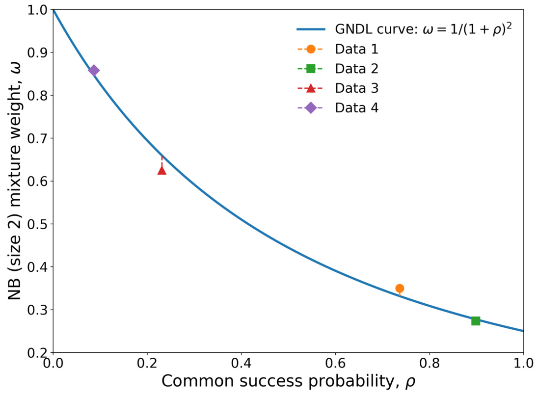
Here, $p_{LR}$ denotes the p-value of the likelihood-ratio test using the statistic $2\Delta \mathcal{l}$ and the ${\chi }_1^2$ reference distribution. Thus, positive information-criterion differences favor the constrained GNDL model. The unrestricted two-parameter mixture produces log-likelihood gains of only 0.000726 and 0.000178 for Data sets 1 and 2, respectively, indicating essentially no empirical gain from independently adjusting the mixing weight in these two samples. For Data set 2, the very large sample size makes the BIC penalty for the additional second parameter particularly strong. For Data set 3, the unrestricted two-parameter model gains only 0.013445 in log-likelihood, and the fitted data point remains close to the GNDL restriction. For Data set 4, the unrestricted mixture again yields a negligible log-likelihood gain (0.000515).

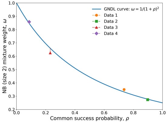
The largest KL divergence from the fitted unrestricted distribution to the fitted GNDL distribution is only about $1.04\times {10}^{-4}$ (Data 3), and the largest total variation distance is about $0.00576$. These quantities provide direct distributional measures of the small estimated cost of the restriction in the four applications, complementing the information-criterion comparisons. Figure 5 shows the GNDL restriction within the unrestricted two-parameter mixture family; the solid curve represents $\omega =1/{\left(1+\rho \right)}^2$. The colored, shape-coded points denote the unrestricted maximum-likelihood estimates from the four real-data applications, while the dashed vertical segments indicate their deviations from the GNDL restriction.

Figure 5. GNDL restriction within the encompassing two-parameter geometric–negative binomial (size 2) mixture family.

8.2. Misspecification Assessment

To assess the cost of the one-parameter coupling, we studied misspecification in the direct $(\rho ,\omega )$ mixture parameterization. The GNDL restriction is the mixing-weight curve defined in Section 2,

$${\omega }_{\mathrm{GNDL}}(\rho )={\displaystyle \frac{1}{{(1+\rho )}^2}}.$$

Departures were defined on the log-odds scale. For an odds ratio OR > 0 relative to the GNDL mixing odds, the unrestricted weight ${\omega }_{\mathrm{OR}}$ satisfies

$${\displaystyle \frac{{\omega }_{\mathrm{OR}}}{1-{\omega }_{\mathrm{OR}}}}=\mathrm{OR}·{\displaystyle \frac{{\omega }_{\mathrm{GNDL}}\left(\rho \right)}{1-{\omega }_{\mathrm{GNDL}}\left(\rho \right)}},$$

or, equivalently,

$${\omega }_{\mathrm{OR}}={\displaystyle \frac{\mathrm{OR}·{\omega }_{\mathrm{GNDL}}\left(\rho \right)}{1-{\omega }_{\mathrm{GNDL}}\left(\rho \right)+\mathrm{OR}·{\omega }_{\mathrm{GNDL}}\left(\rho \right)}}.$$

OR = 1 recovers GNDL exactly, whereas values below and above 1 generate departures on opposite sides of the curve. We used OR $\in \{1/2,1/\surd 2,1,\surd \mathrm{2,2}\}$, a set symmetric on the log-odds scale about 1. This symmetric design provides two matched levels of departure on each side of the exact GNDL case, allowing the effect of increasing misspecification to be assessed systematically. Likelihood-ratio assessments of restricted versus extended discrete models have been used in related count-distribution studies [23,24,25]. For the population-level assessment, we used $\rho \in \{0.1,0.5,0.9\}$. For each ($\rho$, OR), let $f(y;\rho ,{\omega }_{\mathrm{OR}})$ denote the unrestricted probability mass function defined in Section 2, and let $p(y;\alpha )$ denote the GNDL probability mass function defined in Equation (1). The KL-projection parameter was defined by

$${\alpha }_{\mathrm{KL}}(\rho ,\mathrm{OR})=\underset{0<\alpha <1}{\arg \min }{D}_{\mathrm{KL}}[f(·;\rho ,{\omega }_{\mathrm{OR}})\parallel p(·;\alpha )],$$

Minimum KL is the minimized divergence above. The corresponding $d_{\mathrm{TV}}$ is the total variation distance between the unrestricted distribution and its KL-projection GNDL distribution. KL divergence and total variation are established discrepancy measures in count and discrete-distribution studies [26,27].

$$d_{\mathrm{TV}}={\displaystyle \frac{1}{2}}{\sum }_{y=0}^{\mathrm{\infty }}\left|f(y;\rho ,{\omega }_{\mathrm{OR}})-p(y;{\alpha }_{\mathrm{KL}})\right|.$$

At OR = 1, the unrestricted point lies on the GNDL curve, ${\alpha }_{\mathrm{KL}}=\rho$, and both Minimum KL and $d_{\mathrm{TV}}$ are exactly zero by construction. The Monte Carlo assessment used $\rho \in \{0.1,0.5,0.9\}$, $n\in \{50,200,500\}$, and 1000 replications per scenario, giving 45 scenarios and 45,000 simulated samples. Each sample was fitted by GNDL and the unrestricted mixture; exact $\omega =0$ and $\omega =1$ boundary candidates were retained, and no replication was discarded. We recorded LRT rejection frequencies and AIC/BIC GNDL-selection frequencies; these information criteria are standard in count-model comparisons [5]. In each sample-size column of Table 16, entries are reported in the order LRT/AIC/BIC, where LRT denotes the empirical rejection frequency at the 5% level and AIC/BIC denote the frequencies with which GNDL is selected. At OR = 1, Minimum KL and $d_{\mathrm{TV}}$ are zero and AIC/BIC usually select the parsimonious GNDL model. Away from the curve, the cost depends on the parameter region and sample size. For $\rho =0.1$ and OR = 0.5, the LRT rejection rate increases from 0.066 at $n=50$ to 0.183 at $n=200$ and 0.367 at $n=500$, while AIC selection of GNDL falls from 0.811 to 0.632 and 0.418. At $\rho =0.9$, even the largest examined departures yield very small Minimum KL and $d_{\mathrm{TV}}$ values and remain difficult to distinguish statistically. Thus, the restriction is inexpensive near the GNDL curve but becomes detectably inadequate when departures are consequential and information increases. LRT rejection frequencies are treated as a secondary finite-sample diagnostic because unrestricted MLEs can occur at $\omega =0$ or $\omega =1$, making the usual ${\chi }_1^2$ reference approximation less reliable in those samples. The main interpretation therefore rests on Minimum KL, $d_{\mathrm{TV}}$ and AIC/BIC selection.

Table 16. Misspecification results for the complete Monte Carlo design.

$\mathit{\rho }$	OR	Minimum KL	${\mathit{d}}_{\mathbf{TV}}$	n = 50 LRT/AIC/BIC	n = 200 LRT/AIC/BIC	n = 500 LRT/AIC/BIC
0.1	$1/2$	0.002813	0.027206	0.066/0.811/0.937	0.183/0.632/0.905	0.367/0.418/0.796
	$1/\sqrt{2}$	0.000637	0.012709	0.049/0.832/0.953	0.085/0.795/0.961	0.113/0.718/0.963
	1	0	0	0.024/0.842/0.978	0.049/0.834/0.978	0.063/0.835/0.986
	$\sqrt{2}$	0.000473	0.010590	0.024/0.823/0.977	0.076/0.797/0.972	0.101/0.733/0.962
	2	0.001573	0.019045	0.019/0.818/0.984	0.127/0.712/0.933	0.244/0.553/0.878
0.5	$1/2$	0.000413	0.011957	0.005/0.932/0.996	0.025/0.841/0.995	0.065/0.781/0.988
	$1/\sqrt{2}$	0.000134	0.006922	0.010/0.922/0.991	0.029/0.845/0.989	0.045/0.827/0.994
	1	0	0	0.007/0.907/0.995	0.041/0.849/0.986	0.043/0.847/0.989
	$\sqrt{2}$	0.000194	0.008572	0.017/0.893/0.984	0.065/0.817/0.977	0.078/0.783/0.982
	2	0.000858	0.018186	0.030/0.850/0.972	0.097/0.742/0.962	0.148/0.670/0.945
0.9	$1/2$	$5.24\times {10}^{-6}$	0.000574	0.000/1.000/1.000	0.000/0.997/1.000	0.000/0.983/1.000
	$1/\sqrt{2}$	$1.94\times {10}^{-6}$	0.000361	0.000/1.000/1.000	0.000/0.999/1.000	0.000/0.976/1.000
	1	0	0	0.000/1.000/1.000	0.000/0.995/1.000	0.000/0.968/1.000
	$\sqrt{2}$	$3.93\times {10}^{-6}$	0.000556	0.000/1.000/1.000	0.000/0.999/1.000	0.001/0.958/1.000
	2	$2.09\times {10}^{-5}$	0.001337	0.000/1.000/1.000	0.000/0.997/1.000	0.000/0.951/1.000

9. Conclusions

This paper studied the geometric–natural discrete Lindley (GNDL) distribution as a fully discrete one-parameter model for overdispersed and positively skewed count data. The model arises from a nested geometric–NDL construction. Equivalent geometric–negative binomial latent-stage and random-sum representations were also established, providing direct probabilistic interpretations and an exact mechanism for generating observations from the distribution without introducing an additional parameter.

Several distributional and reliability properties of the GNDL model were derived in closed form. These include the probability-generating and moment-generating functions, moments, dispersion measures, survival and hazard functions, and stochastic-ordering results. The distribution is overdispersed throughout its parameter space. Its probability mass function is log-concave and unimodal, and its discrete hazard rate is increasing. Consequently, the model belongs to important aging classes, including the increasing-failure-rate and decreasing-mean-residual-life classes.

Four estimation procedures were investigated: maximum likelihood, method of moments, method of proportions, and minimum chi-square estimation. The simulation results showed that estimation accuracy generally improves as the sample size increases. MLE and MOM exhibited nearly identical finite-sample behavior and provided the most consistently favorable precision. PE frequently offered better centering, particularly for moderate and large parameter values, but was sensitive to samples containing no zero observations. MCS remained numerically stable and improved with increasing sample size, although it displayed a persistent finite-sample tendency to underestimate the parameter. These findings reveal a clear trade-off between centering and precision rather than the uniform dominance of a single estimator.

The four real-data applications demonstrated that the GNDL distribution provides acceptable goodness of fit for grouped count data and discrete lifetime observations. It attained favorable information-criterion values in all applications while retaining a parsimonious one-parameter structure. Nevertheless, its advantages over the closest competing models were modest in several cases. The empirical findings should therefore be interpreted as evidence of competitive and parsimonious performance rather than universal superiority.

GNDL is a one-parameter constrained submodel of the published two-parameter TNDL family and admits an equivalent geometric–negative binomial (size 2) mixture representation with a common success probability. Its defining restriction couples the common success probability and the two-stage mixture weight. In the four applications studied here, the unrestricted model yields negligible likelihood gains, whereas both AIC and BIC favor the constrained GNDL model; the fitted unrestricted points lie close to the GNDL curve, and the corresponding fitted unrestricted distributions are also close to their GNDL counterparts in KL divergence and total-variation distance. The misspecification study shows, however, that the adequacy of this restriction is conditional rather than universal: sufficiently strong departures from the curve become detectable as sample information increases. Accordingly, GNDL should be viewed as a tractable and empirically testable parsimonious restriction whose suitability depends on whether its parameter coupling is compatible with the data.

References

- Lindley, D.V. Fiducial distributions and Bayes’ theorem. J. R. Stat. Soc. Ser. B (Methodol.) 1958, 20, 102–107. [Google Scholar] [CrossRef] [Scilit]
- Ghitany, M.E.; Atieh, B.; Nadarajah, S. Lindley distribution and its application. Math. Comput. Simul. 2008, 78, 493–506. [Google Scholar] [CrossRef] [Scilit]
- Gómez-Déniz, E.; Calderín-Ojeda, E. The discrete Lindley distribution: Properties and applications. J. Stat. Comput. Simul. 2011, 81, 1405–1416. [Google Scholar] [CrossRef] [Scilit]
- Al-Babtain, A.A.; Ahmed, A.H.N.; Afify, A.Z. A new discrete analog of the continuous Lindley distribution, with reliability applications. Entropy 2020, 22, 603. [Google Scholar] [CrossRef] [Scilit]
- Shafiq, S.; Khan, S.; Marzouk, W.; Gillariose, J.; Jamal, F. The binomial–natural discrete Lindley distribution: Properties and application to count data. Math. Comput. Appl. 2022, 27, 62. [Google Scholar] [CrossRef] [Scilit]
- Shanker, R.; Mishra, A. A two-parameter Poisson–Lindley distribution. Int. J. Stat. Syst. 2014, 9, 79–85. [Google Scholar]
- Fisher, R.A. The effect of methods of ascertainment upon the estimation of frequencies. Ann. Eugen. 1934, 6, 13–25. [Google Scholar] [CrossRef] [Scilit]
- Rao, C.R. On discrete distributions arising out of methods of ascertainment. In Classical and Contagious Discrete Distributions; Patil, G.P., Ed.; Statistical Publishing Society: Calcutta, India, 1965; pp. 320–332. [Google Scholar]
- Patil, G.P.; Rao, C.R. Weighted distributions and size-biased sampling with applications to wildlife populations and human families. Biometrics 1978, 34, 179–189. [Google Scholar] [CrossRef] [Scilit]
- Shanker, R.; Mishra, A. A two-parameter Lindley distribution. Stat. Transit. New Ser. 2013, 14, 45–56. [Google Scholar] [CrossRef] [Scilit]
- Sankaran, M. The discrete Poisson–Lindley distribution. Biometrics 1970, 26, 145–149. [Google Scholar] [CrossRef] [Scilit]
- Kemp, A.W. Classes of discrete lifetime distributions. Commun. Stat. Theory Methods 2004, 33, 3069–3093. [Google Scholar] [CrossRef] [Scilit]
- Shaked, M.; Shanthikumar, J.G. Stochastic Orders; Springer: New York, NY, USA, 2007. [Google Scholar] [CrossRef] [Scilit]
- Khan, M.S.A.; Khalique, A.; Abouammoh, A.M. On estimating parameters in a discrete Weibull distribution. IEEE Trans. Reliab. 1989, 38, 348–350. [Google Scholar] [CrossRef] [Scilit]
- Barbiero, A.; Hitaj, A. A discrete version of the half-logistic distribution based on the mimicking of the probability density function. J. Indian. Soc. Probab. Stat. 2024, 25, 373–394. [Google Scholar] [CrossRef] [Scilit]
- Barbiero, A. Least-squares and minimum chi-square estimation in a discrete Weibull model. Commun. Stat. Simul. Comput. 2017, 46, 8028–8048. [Google Scholar] [CrossRef] [Scilit]
- Lawless, J.F. Statistical Models and Methods for Lifetime Data, 2nd ed.; Wiley: Hoboken, NJ, USA, 2003. [Google Scholar]
- Gossiaux, A.M.; Lemaire, J. Méthodes d’ajustement de distributions de sinistres. Bull. Assoc. Swiss Actuar. 1981, 81, 87–95. [Google Scholar]
- Puig, P.; Valero, J. Count data distributions: Some characterizations with applications. J. Am. Stat. Assoc. 2006, 101, 332–340. [Google Scholar] [CrossRef] [Scilit]
- Altun, E.; Cordeiro, G.M.; Ristić, M.M. An one-parameter compounding discrete distribution. J. Appl. Stat. 2022, 49, 1935–1956. [Google Scholar] [CrossRef] [Scilit]
- Bakouch, H.S.; Aghababaei Jazi, M.; Nadarajah, S. A new discrete distribution. Statistics 2014, 48, 200–240. [Google Scholar] [CrossRef] [Scilit]
- Nakagawa, T.; Osaki, S. The discrete Weibull distribution. IEEE Trans. Reliab. 1975, R-24, 300–301. [Google Scholar] [CrossRef] [Scilit]
- Chakraborty, S.; Bhati, D. Analysis of count data by transmuted geometric distribution. J. Stat. Theory Appl. 2019, 18, 450–463. [Google Scholar] [CrossRef] [Scilit]
- Roy, S.; Tripathi, R.C.; Balakrishnan, N. A Conway–Maxwell–Poisson type generalization of hypergeometric distribution. Mathematics 2023, 11, 762. [Google Scholar] [CrossRef] [Scilit]
- Roy, S.; Tripathi, R.C.; Balakrishnan, N. A Conway Maxwell Poisson type generalization of the negative hypergeometric distribution. Commun. Stat. Theory Methods 2020, 49, 2410–2428. [Google Scholar] [CrossRef] [Scilit]
- Rodríguez-Avi, J.; Olmo-Jiménez, M.J. A regression model for overdispersed data without too many zeros. Stat. Pap. 2017, 58, 749–773. [Google Scholar] [CrossRef] [Scilit]
- Adell, J.A.; Jodrá, P. Exact Kolmogorov and total variation distances between some familiar discrete distributions. J. Inequal. Appl. 2006, 2006, 64307. [Google Scholar] [CrossRef] [Scilit]
Disclaimer/Publisher’s Note: The statements, opinions and data contained in all publications are solely those of the individual author(s) and contributor(s) and not of MDPI and/or the editor(s). MDPI and/or the editor(s) disclaim responsibility for any injury to people or property resulting from any ideas, methods, instructions or products referred to in the content. |
© 2026 by the authors. Licensee MDPI, Basel, Switzerland. This article is an open access article distributed under the terms and conditions of the Creative Commons Attribution (CC BY) license.