


Abstract
This paper develops a Banach space-valued approximation framework based on symmetrized neural network (SNN) operators generated by a deformation-dependent sigmoidal activation function. Symmetry is introduced directly at the activation level through a reciprocal-deformation mechanism, yielding a positive, even, normalized, and localized density kernel satisfying the partition of unity. The resulting construction provides normalized compact-interval and whole-line quasi-interpolation operators for Banach space-valued functions. Quantitative pointwise and uniform convergence estimates are established through the first modulus of continuity and are extended to higher-order and Caputo–Bochner fractional approximation. Numerical diagnostics support the theoretical kernel properties, and fractional approximation experiments compare the SNN and classical NN operators under common computational conditions. A controlled blind-prediction experiment on a synthetic monthly temperature-like series uses a strict fit–validation–test protocol and a parameter-matched operator comparison, with seasonal ARIMA and MLP models as external baselines. Across five independent realizations, the SNN attains the best mean predictive performance, with , NMAE , and NRMSE . A vector-valued experiment in further illustrates the non-scalar applicability of the Banach space framework. In addition, the normalized SNN kernel weights provide an intrinsic node-level interpretation mechanism without requiring an external post hoc explainability method.
Keywords:
symmetrized neural network operators; Banach space-valued approximation; modulus of continuity; fractional approximation; Caputo–Bochner derivative; kernel-based explainability; numerical approximation MSC:
26A33; 41A17; 41A25; 41A30; 46B25
1. Introduction
Quantitative approximation theory provides a rigorous analytical foundation for studying the convergence behavior of constructive operators and their error estimates. In particular, explicit pointwise and uniform bounds are essential not only for proving that an approximation process is convergent, but also for understanding how rapidly this convergence occurs [1]. Within this general framework, ordinary and fractional neural network approximation has become an active research direction, especially for Banach space-valued functions and deformation-dependent activation functions [2,3]. Approximation operators generated by sigmoid-type functions also form a natural bridge between classical approximation theory and neural network-type computational models [4,5].
These developments are also connected with the modern approximation-theoretic foundations of neural networks. Quantitative error and complexity bounds for deep neural networks have been established for smooth and Sobolev-regular function classes [6,7]. These modern developments complement the historical neural-network foundations [8,9,10] and provide a more direct theoretical context for the approximation processes considered here.
From the broader perspective of constructive approximation, positive linear operators and sampling-type processes provide important frameworks for quantitative convergence analysis. Recent Bernstein-type developments include modified -Bernstein–Bézier operators and Stancu variants with shifted knots, for which Korovkin-type convergence, moduli of smoothness, Peetre K-functionals, and Voronovskaja-type estimates have been studied [11,12]. Related sampling Kantorovich operators extend this constructive viewpoint to sampling-based approximation, including direct, inverse, and saturation results [13]. Together with sigmoidal approximation operators [14], these developments place the present SNN construction within the broader theory of constructive approximation operators.
A further motivation for the present study arises from the role of symmetry in approximation and learning. Symmetry can reduce structural complexity, improve representational efficiency, and reorganize the local weight distribution of an approximation operator. In kernel regression, invariance may provide a measurable gain in sample complexity [15]. Moreover, symmetrized neural network approximation over infinite domains has shown that symmetry can be incorporated constructively into neural-network-type approximation operators [16]. Related ideas have also appeared in symmetric neural network architectures [17], symmetric neural network theory [18], affine symmetries and neural network identifiability [19], symmetry learning in deep networks [20], and the representation of symmetric or antisymmetric functions [21]. These studies indicate that symmetry is not only a geometric constraint, but also a useful structural principle for approximation and learning mechanisms.
The present paper adopts a distinct and structurally direct approach to symmetry. Instead of imposing symmetry directly on a multi-layer neural network architecture or on the output of an already constructed approximation operator, we introduce symmetry at the activation-function level. More precisely, we start with a deformation-dependent sigmoidal activation function and construct its associated density kernel. Then, using the reciprocal deformation of the activation parameter, we define a symmetrized activation and derive the corresponding activation-induced density kernel. Hence, the symmetric density kernel is not artificially imposed after the approximation operator has been formed; rather, it is generated directly from the reciprocal-deformation symmetry of the activation function itself. This construction is related to the SNN approximation approach in [16], while the activation framework is motivated by ordinary and fractional NN approximation results [2,3] and related hyperbolic-type activation structures [5,22].
The resulting symmetrized density kernel is positive, even, normalized, localized, and satisfies the partition of unity property. These properties provide the analytical basis for defining normalized NN approximation operators on compact intervals and quasi-interpolation operators on the whole real line. In the compact-interval setting, however, only sampling nodes lying in are admissible, so the corresponding finite kernel sum does not need to equal one, even though the full infinite sum satisfies the partition of unity. This loss of kernel mass is particularly relevant near the endpoints, where part of the density may fall outside the admissible sampling range. Consequently, an explicit normalization denominator is required in the compact-interval operator.
The Banach space-valued formulation places this construction within a broader functional-analytic setting and allows the theory to accommodate vector-valued, function-valued, and other structured outputs rather than being restricted to scalar-valued functions. Within the general framework of quantitative approximation [1], Banach space-valued NN approximation based on parametrized and deformed activation functions has previously yielded ordinary and fractional approximation estimates [2,3]. Related developments include approximation operators generated by sigmoidal functions [4], SNN approximation over infinite domains [16], and generalized NN operators [23]. The present approach is connected with these frameworks but differs in its structural construction: the generating activation is paired with its reciprocal-deformation counterpart and symmetrized before the associated density kernel is formed. Moreover, in contrast to the infinite-domain SNN setting in [16], the present framework treats both normalized compact-interval operators and whole-line quasi-interpolation operators. Thus, it extends this line of Banach space-valued approximation research through a reciprocal-deformation symmetry mechanism introduced directly at the activation level.
Within this setting, the first modulus of continuity serves as the principal measure of local regularity and yields quantitative estimates that relate the approximation error to the sampling level, kernel localization, and regularity of the target function. The analysis first establishes pointwise and uniform approximation results and is then extended to higher-order and Caputo–Bochner fractional approximation. In this way, the proposed SNN framework covers both ordinary and fractional smoothness settings within a unified Banach space-valued approximation structure.
In parallel, recent numerical approximation research reflects the growing interaction between fractional calculus and computational methods. Finite-element schemes have been developed for variable-order fractional diffusion problems [24], while neural-network-based numerical methods have been proposed for generalized Caputo-type fractional differential equations [25]. Related approximation results for residual neural networks further demonstrate the relevance of modern neural architectures to fractional differential models [26]. These developments provide a contemporary numerical context for the Caputo–Bochner fractional approximation framework considered in the present study.
Recent independent contributions further broaden the operator-theoretic context of neural network approximation. Best-order and inverse approximation results for classical and Kantorovich-type neural network operators have been established in connection with Lipschitz regularity classes [27]. Durrmeyer-type neural network operators generated through sigmoidal density functions have also been studied with respect to pointwise and uniform convergence, quantitative approximation estimates, and -approximation [28]. Feedforward neural network operators constructed from generalized sigmoidal functions provide further quantitative approximation-rate results based on moduli of continuity [29]. Deep Kantorovich-type neural network operators extend this constructive setting to multilayer structures, with density results in continuous and spaces [30]. Related contemporary developments include quantitative approximation by neural network operators generated through hyperbolic tangent functions [31], sampling Kantorovich approximation in Sobolev and fractional Sobolev spaces [32], and Kantorovich-type neural network operators activated by smooth ramp functions, including direct and converse approximation results [33]. Multivariate neural network operators based on smooth ramp activations further extend this line of research to higher-dimensional approximation settings [34]. Together, these studies illustrate the continuing development of constructive neural network approximation across different activation mechanisms, operator structures, function spaces, and dimensions.
The connection between constructive neural network operators and fractional approximation has also been developed in directions that are particularly relevant to the present setting. Neural network operators for generalized multivariate fractional integrals equipped with a vector-valued function have been investigated together with quantitative approximation estimates [35]. In addition, Riemann–Liouville fractional-integral-type exponential sampling Kantorovich series have been introduced and analyzed through convergence rates and Voronovskaja-type asymptotic results [36]. These works provide complementary contemporary examples of how fractional structures, sampling mechanisms, and neural-network-type operators can be combined within constructive approximation theory. They are included here to broaden the modern fractional approximation context and are not used as theoretical premises for the results established in the present paper.
Building on this analytical framework, the numerical study evaluates the proposed kernel through structural diagnostics, fractional approximation experiments, and a controlled blind-prediction test. The latter uses a strict fit–validation–test split, a parameter-matched comparison of the SNN and classical NN operators under , seasonal ARIMA and MLP baselines, and five independent synthetic realizations.
A further feature of the proposed operator is its transparency. Since the operator is formulated as a normalized positive linear combination of sampled function values, the relative influence of each sampling node is explicitly quantified by its corresponding normalized kernel weight. These non-negative weights sum to one and can therefore be inspected directly to determine which nodes exert the strongest local influence on a given prediction. This provides an intrinsic node-level interpretation mechanism, which is particularly relevant when approximation accuracy and interpretability are considered together.
The main contributions of this paper can be summarized as follows:
- A reciprocal-deformation mechanism is introduced to generate symmetry directly at the activation level.
- The induced density kernel is shown to be positive, even, normalized, localized, and compatible with the partition of unity.
- New compact-interval and quasi-interpolation SNN operators are developed for Banach space-valued approximation.
- Quantitative pointwise, uniform, higher-order, and Caputo–Bochner fractional estimates are established.
- A controlled blind-prediction experiment is conducted using a strict fit–validation–test protocol and a parameter-matched comparison of the SNN and classical NN operators. Seasonal ARIMA and MLP models are included as external baselines, and five independent synthetic realizations are used to assess robustness.
- The normalized SNN kernel coefficients provide an intrinsic node-level interpretation mechanism, allowing the influence of individual sampling nodes on an unseen prediction to be inspected directly.
- A vector-valued numerical demonstration in provides an explicit non-scalar realization of the Banach space-valued framework, with approximation errors evaluated in the corresponding vector norm.
The paper is organized as follows. Section 2 constructs the deformation-dependent activation function, its reciprocal-deformation counterpart, and the resulting symmetrized activation-induced density kernel. It also establishes the fundamental kernel properties, including positivity, evenness, normalization, partition of unity, and localization, supported by numerical diagnostics.
Section 3 introduces the compact-interval and whole-line SNN approximation operators, establishes pointwise and uniform approximation estimates for Banach space-valued functions, and presents the controlled blind-prediction experiment, including parameter-matched operator comparison, external forecasting baselines, robustness analysis, and node-level interpretation.
Section 4 develops the higher-order and Caputo–Bochner fractional approximation theory.
Section 5 presents the numerical approximation experiments, including fractional classical–SNN comparisons, fractional Taylor remainder validation, error analysis, and a vector-valued demonstration in .
Finally, Section 6 summarizes the main theoretical and numerical findings, discusses the dimensional scalability of possible multivariate extensions, and outlines directions for future research.
2. Symmetric Activation-Induced Density Kernel
Our basic deformation-dependent sigmoidal activation function is defined by
where and . Here, is the shape parameter and t is the deformation coefficient. For related constructions, we refer to [2,3,5].
The density kernel generated by is given by
Since is increasing on , the positivity in (2) follows immediately.
We now introduce the reciprocal-deformation structure at the activation-function level. The reciprocal-deformation activation is
A direct computation gives
Indeed,
Motivated by (3), we define the symmetrized reciprocal-deformation activation function by
Equivalently,
From (3) and (6), we obtain the central symmetry relation
This activation-level symmetry will induce an even density kernel.
We define the density kernel induced by the symmetrized activation as
This is the symmetrized density kernel used throughout the paper.
Let us now show that F is exactly the average of the two reciprocal-deformation density kernels. By using (6), we have
By the definition of in (2), this gives
Hence, F is obtained directly from the symmetrized reciprocal-deformation activation .
Moreover, F is an even density kernel. Indeed, using (8), we get
That is,
Therefore, the activation-level central symmetry of induces the y-axis symmetry of the density kernel F.
Lemma 1.
Let and . The symmetric activation-induced density kernel F satisfies the following two properties:
and
Consequently, F is a normalized density kernel.
Proof.
By Theorem 18.1, p. 458 of [3], for all and , we have
Since the symmetric activation-induced density kernel has the representation
we obtain
This proves (14).
Next, by Theorem 18.2, p. 459 of [3], for , we have
Again, using the representation of F, we get
This proves (15).
Since F is positive and satisfies by construction, it follows that F is a positive, even, normalized density kernel. □
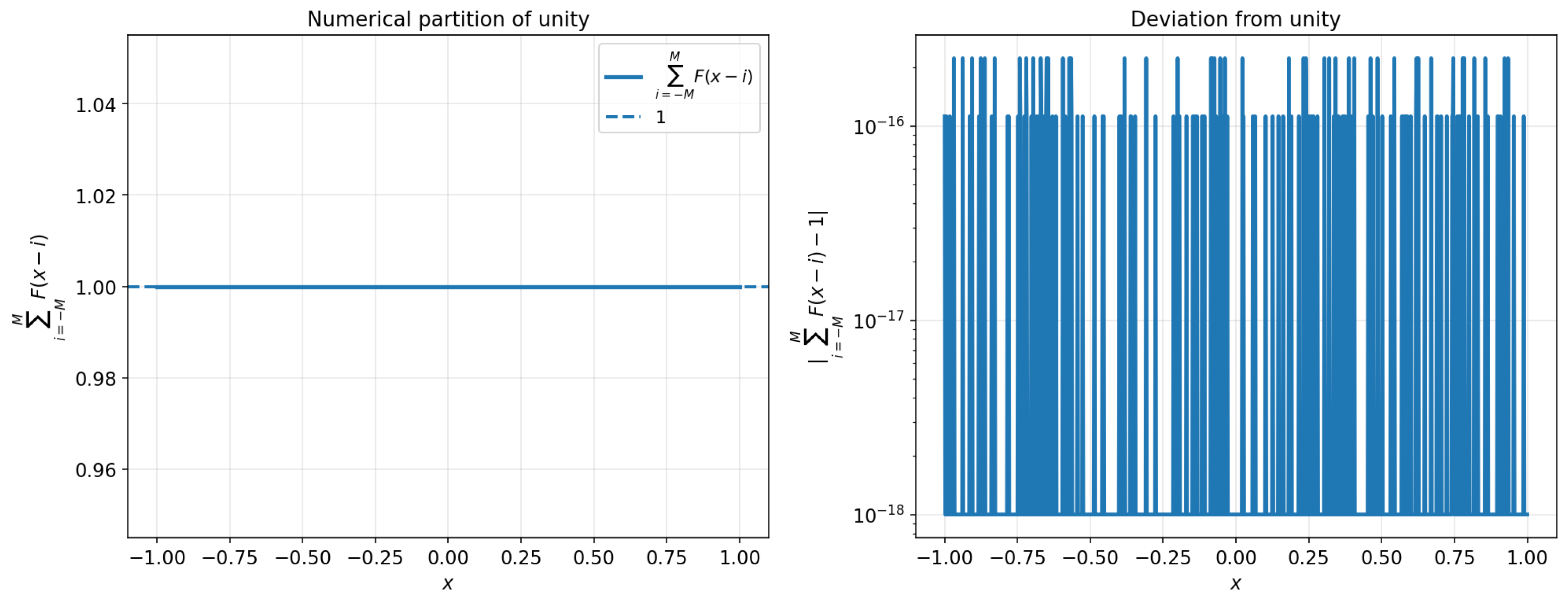
- The preceding lemma establishes that the activation-induced density kernel F satisfies the partition of unity property and is normalized. To complement this theoretical result, we provide a numerical illustration of the discrete partition of unity property. In the computation, the infinite series is approximated by the truncated sum where , which is taken sufficiently large, so that the omitted tail terms for become numerically negligible. denotes the partition of unity residual. The corresponding pointwise deviation from unity is measured byThe right panel shows the pointwise difference between the truncated sum and 1. This difference remains very small on the plotted interval, indicating that the partition of unity property is numerically preserved. Thus, Figure 1 supports the use of F as a normalized density kernel in the proposed discrete operator framework.
Figure 1.
Numerical illustration of the partition of unity property established in Lemma 1.
Lemma 2.
Let and let be such that . For , define
Then, for every , the symmetric activation-induced density kernel F satisfies
Proof.
Lemma 2 provides the theoretical tail estimate for the symmetric activation-induced density kernel F. We now complement this result with numerical diagnostics. These computations verify the activation-level symmetry, the evenness of the induced density kernel, the partition of unity, the finite-interval normalization, and the tail decay behavior.
2.1. Numerical Verification of the Activation-Symmetry Mechanism
The aim of this experiment is not to introduce a new approximation operator, but to numerically illustrate the activation-level origin of the symmetric density kernel F. In particular, we verify that the symmetrized activation satisfies the central symmetry relation (8), and that the density kernel induced by this activation is even, normalized, and localized.
We first illustrate the activation-level origin of the proposed symmetric density kernel. For this purpose, we consider together with . In the numerical illustration, we take , and plot the three activation functions
on the interval .
Figure 2 shows that the proposed symmetrization is imposed before the density kernel is constructed. Thus, the symmetric density kernel is not introduced only at the density level; rather, it is induced from the activation-level symmetrization
Figure 2.
Activation-level reciprocal-deformation symmetry.
2.2. Numerical Diagnostics for the Symmetric Density Kernel
We now give a short numerical diagnostic test for the symmetric activation-induced density kernel F. The purpose is to support the normalization, symmetry, partition of unity, and tail-decay properties proved above. Throughout this test, we take , , , , , and use a uniform computational grid consisting of points over the interval . Here, determines the finite integration interval, specifies the grid resolution used for the pointwise activation- and density-based diagnostics, and is used as the truncation level in the discrete partition-of-unity sum. Since F is localized around the origin and its tails decay rapidly, these choices provide sufficient resolution and truncation accuracy for the present numerical verification.
All numerical diagnostics were implemented in Python 3.13 using NumPy double-precision floating-point arithmetic (IEEE 754 binary64, float64). The stable logistic evaluation was performed using scipy.special.expit when available. Accordingly, residuals of order in the activation-symmetry, density-symmetry, and partition-of-unity diagnostics are interpreted as floating-point round-off effects at machine precision rather than as violations of the corresponding analytical identities.
Table 1 shows that the activation-symmetry, density-symmetry, and partition of unity errors are all at the level of machine precision. The integral of F over is close to one; the small deviation is expected because the theoretical normalization is defined over the whole real line, whereas the numerical integral is computed on a finite interval.
Table 1.
Numerical diagnostics for the activation-symmetry mechanism and the induced density kernel F.
Next, we examine the tail behavior of F. For a fixed and , we compute
and compare it with the theoretical upper bound
Table 2 and Figure 3 confirm the localization behavior stated in Lemma 2. The numerical tail mass decreases rapidly as n increases, from approximately for to for . Moreover, remains below the theoretical bound for all tested values of n, with staying between approximately and .
Table 2.
Numerical tail mass , theoretical bound , and the ratio .
Figure 3.
Tail decay of the symmetric activation-induced density kernel.
2.2.1. Activation-Level Central Symmetry Error
After illustrating the activation-level construction of , we next verify its central symmetry property numerically. Recall that the symmetrized reciprocal-deformation activation satisfies (8). To quantify this property, we compute the activation-symmetry error
In the numerical experiment, we use and take . A value of close to machine precision confirms that the activation-level central symmetry is numerically preserved.
The left panel provides a direct visual verification of the activation-level central symmetry relation (8). Indeed, the two curves and are almost indistinguishable on the plotted interval. This confirms that the symmetrized activation is not symmetric with respect to the y-axis in the usual even-function sense. Rather, it is centrally symmetric with respect to the point . In other words, the values of at two opposite points x and complement each other to one.
The right panel gives a numerical residual corresponding to (27). More precisely, it plots the pointwise error
If the identity (27) were violated in a meaningful way, this residual would take visibly large values. However, the plotted residual remains extremely small. Since the vertical axis is logarithmic, the apparent oscillations in the right panel should not be interpreted as structural deviations from symmetry. They only reflect round-off effects arising from finite-precision floating-point arithmetic. In the present computation, the residual stays between approximately and , which is essentially at machine precision.
Therefore, Figure 4 numerically confirms that the central symmetry relation (8) holds up to numerical precision. This is important for the present construction, because the evenness of the induced density kernel F is a consequence of this activation-level symmetry. Thus, the symmetry is first imposed at the activation-function level, and the symmetric density kernel is subsequently generated from this activation.
Figure 4.
Numerical verification of the activation-level central symmetry.
2.2.2. Construction and Properties of the Even Density Kernel Induced by Symmetrized Activation
We next illustrate the density kernel induced by the symmetrized activation . Recall that this density kernel is defined by F. Since the symmetrized activation satisfies the central symmetry relation, the induced density kernel is expected to satisfy
The left panel shows that the density kernel F has a symmetric bell-shaped profile centered at the origin. The curves and coincide on the whole plotted interval. This means that the density kernel induced by the symmetrized activation is even with respect to the y-axis.
The right panel provides a zoomed view around the central part of the kernel, where the density takes its largest values. This zoom is useful because the two curves and overlap almost exactly in the full-scale plot. The coincidence remains visible also near the peak of the density, showing that the symmetry is not only a tail behavior but is preserved throughout the main mass of the kernel.
Figure 5 supports the main idea of the proposed construction: the symmetry is first imposed at the activation-function level through , and then transferred to the induced density kernel F. Therefore, the evenness of F is not imposed artificially at the density level; it is a direct consequence of the activation-level central symmetry.
Figure 5.
Even density kernel induced by the symmetrized activation.
Figure 6 gives a quantitative numerical verification of the evenness of the activation-induced density kernel F. While Figure 5 visually confirms the overlap of and , this figure measures the pointwise residual .
Figure 6.
Numerical density-symmetry error associated with the induced density kernel.
The residual remains between approximately and on the plotted interval. Hence, the observed deviations are not structural errors but only round-off effects caused by finite-precision arithmetic. The logarithmic vertical scale is used solely to make these extremely small discrepancies visible; the apparent oscillations should therefore not be interpreted as a loss of symmetry.
Consequently, Figure 6 numerically confirms that is preserved up to machine precision. Together, Figure 5 and Figure 6 support the main mechanism of the proposed construction: the central symmetry of the symmetrized activation is transferred to the density level, producing an even density kernel F.
Theorem 1.
Let , , and let F be the symmetric activation-induced density kernel defined by Assume that there exist and such that the finite denominator estimates for and hold. Define
Then, for every and every satisfying we have
Proof.
By the finite denominator estimate, applied to , we have
Hence,
Similarly, applying the same estimate to , we obtain
Using the representation we get
Therefore,
which proves the assertion. □
The key observation behind the following remark is that the partition of unity holds for the full infinite lattice, whereas restricting the summation to those sampling nodes that lie in a compact interval may remove part of the kernel mass.
Remark 1.
(i) More specifically, Remark 18.5, p. 460 of [3], states that the finite kernel sum associated with the compact interval need not converge to the partition-of-unity value 1 as . In particular, for at least some , one may have
Similarly, for some , one may have
where . Therefore, in general, the corresponding finite sum associated with the averaged density need not converge to 1. Namely,
In particular, even if
we still have
because this gives
This follows from (34). Hence, although the full infinite sum satisfies the partition of unity property, the finite compact-interval sum is not necessarily equal to 1. Consequently, the normalization denominator in the compact-interval operators is essential and cannot be omitted in general.
(ii) For sufficiently large and for any compact interval with , we have
Moreover, since F is non-negative and satisfies the full partition of unity, we obtain
Finally,
Thus, the finite summation range corresponds exactly to the sampling nodes lying in the compact interval .
3. Pointwise and Uniform Approximation by Symmetrized Neural Network (SNN) Operators
Building on the symmetric activation-induced density kernel F constructed in Section 2, we now pass from the kernel framework to the associated approximation operators. The positivity, symmetry, normalization, partition of unity, and localization properties established above provide the analytic basis for the SNN operators considered in this section.
Let be a Banach space. We introduce both the normalized compact-interval SNN operator and its whole-line quasi-interpolation counterpart, and then study their pointwise and uniform approximation properties for Banach space-valued functions.
Notation 1.
As in [1], let f be a Y-valued function defined on a set . We denote its first modulus of continuity by
In the special case where , we use the shorter notation For functions whose domain is the whole real line, we shall use the following function spaces:
and
Furthermore, whenever or , the first modulus of continuity satisfies
Definition 1.
For , , and satisfying the Y-valued compact-interval symmetrized neural network operator is defined by
The denominator in (46) is strictly positive by Theorem 1.
Definition 2.
For or , the Y-valued quasi-interpolation symmetrized neural network operator is defined by
We present a set of Y-valued SNN approximations to a function given quantitatively.
Theorem 2.
Let , , and let be such that Assume that , , and . Then
where W is defined as in Lemma 2. Consequently,
In particular,
pointwise and uniformly on .
Proof.
Fix . By Definition 1, we have Since by Theorem 1, we may write
Taking norms and using the positivity of F, we get
Again, by Theorem 1, we have
We split the finite summation range into two parts:
and
For , we have
Hence,
By Lemma 1, Therefore,
For , we use the elementary estimate
Hence,
By Lemma 2,
Therefore,
Combining the estimates over and , we obtain (48). This proves the pointwise estimate.
Since the right-hand side is independent of x, taking the supremum over yields (49). Finally, since , it is uniformly continuous on . Hence,
Moreover, since , , and , we have
Therefore,
and consequently pointwise and uniformly on . This completes the proof. □
Next, we give:
Theorem 3.
Let , , , and . Suppose that satisfies For every , the quasi-interpolation SNN operator satisfies
Moreover,
If, in addition, , then pointwise and uniformly on as .
Proof.
Take an arbitrary . On the whole real line, the kernel F forms a normalized family of weights. Hence, the value may be written as
The quasi-interpolation operator is given by (47). Subtracting the two weighted expressions gives
Since , we obtain
We split the index set according to the distance between the sampling node and the point x. Put
and
The set collects the nearby nodes, while contains the indices lying outside this local neighborhood.
For , one has The modulus of continuity then yields
Accordingly, the local contribution is bounded by
It remains to estimate the part coming from . Since f is bounded on , we have
Thus,
By the tail estimate for F, the last sum is dominated by Consequently,
Adding the estimates for the local and far parts gives (66). This proves the pointwise bound.
The obtained estimate is uniform in x. Taking the supremum over , we get
Now assume . The uniform continuity of f gives Furthermore, , , and imply
Hence,
The convergence of to f, both pointwise and uniformly on , follows immediately. □
High-order approximation then follows.
Theorem 4.
Let , , , , , and . Suppose that satisfies Then, the following assertions hold.
For brevity, set
- (i)
- For every , the compact-interval SNN operator satisfies
- (ii)
- If there exists such thatthen only the Taylor remainder contributes, and
- (iii)
- The corresponding uniform estimate is
- (iv)
- Consequently, pointwise and uniformly on as .
Proof.
Pick . For every admissible integer m, that is, the sampling point lies in the interval . We expand f around x by Taylor’s formula:
where the remainder is controlled by
The compact-interval SNN operator forms a normalized weighted average with weights . Since these weights are non-negative and the denominator is controlled by , we obtain
We now divide the admissible indices into two groups. The first group consists of nodes close to x:
while the second group contains the remaining tail indices:
Let . Then
Thus, for ,
and the Taylor remainder satisfies
Using also the partition of unity property of F, the total contribution of the local indices is at most
It remains to estimate the tail part. For , both x and belong to , so
Consequently,
As for the rest, a rough but adequate estimate
is used. The localization estimate for F gives
Accordingly, the tail contribution is bounded by
Adding the local and tail estimates gives (80).
If and then all Taylor polynomial terms disappear at . The preceding estimate therefore leaves only the remainder part, which gives item .
Taking the supremum over in the pointwise bound replaces by . This gives the uniform estimate in item .
Finally, is continuous on the compact interval , and hence is uniformly continuous. Thus,
Furthermore,
and the tail factor satisfies
The right-hand side of the uniform estimate therefore tends to zero. Hence, pointwise and uniformly on . □
3.1. Data-Driven Application: A Controlled Blind Prediction Experiment
As a data-driven application of the ordinary SNN approximation framework developed in this section, we present a controlled blind-prediction experiment designed to evaluate the predictive behavior of the proposed SNN operator. This application is placed here because it directly uses the compact-interval operators introduced and analyzed in Section 3, and it is distinct from the fractional numerical Examples 1 and 2 presented later in Section 5. The classical NN operator is based on the density kernel , whereas the SNN operator is based on the symmetrized density kernel F. In addition to comparing these two operators, the extended experiment benchmarks the SNN against a seasonal ARIMA model and a multi-layer perceptron (MLP) under the same unseen blind-test setting. All models are evaluated on the same synthetic monthly time series containing seasonality, trend, and random fluctuations. The experiment is further complemented by a multi-seed robustness analysis and a node-level examination of the normalized SNN kernel weights in order to assess both predictive stability and the intrinsic interpretability of the proposed operator.
- Description of the data and prediction task:
The dataset used in this experiment is a synthetic monthly temperature-like time series covering a ten-year period, corresponding to 120 monthly observations. The purpose of this controlled dataset is to examine the predictive behavior of the operators under a signal structure containing seasonal oscillation, a mild increasing trend, and random fluctuations. More precisely, the data are generated by
where 15 is the baseline level, 10 is the seasonal amplitude, represents the annual periodic component, models a mild upward trend, and denotes the random noise term.
Thus, the synthetic series combines periodic seasonal behavior, a gradual long-term trend, and observational variability. To maintain a strictly separated model-selection and evaluation protocol, the first 72 observations, corresponding to months , are used to fit the continuous seasonal trend during hyperparameter optimization. The subsequent 24 observations, corresponding to months , form the validation set used for hyperparameter selection. The final 24 observations, corresponding to months , are kept completely unseen throughout model fitting and hyperparameter selection and are used exclusively for blind-test evaluation.
After the operator hyperparameters have been selected using the fit–validation split, the continuous seasonal trend is refitted using the complete pre-test period consisting of the first 96 observations. The resulting fitted function and the selected operator configurations are then used to generate predictions for the untouched 24-month blind-test interval. Hence, the final two years of the series are not involved in either parameter estimation or hyperparameter selection.
The monthly observations are mapped to the compact interval by
The continuous seasonal trend function used in the fitting and refitting stages is represented by
where
maps the normalized input back to the monthly scale.
The parameters A, , , B, and are estimated using only the observations available at the corresponding fitting stage. No observations from the blind-test interval are used in estimating these parameters.
- Generalized classical NN and SNN operators:
For the comparison, we use the generalized compact-interval form of the two operators, in line with the generalized NN operator framework developed in [23]. The classical NN operator is defined by
whereas the symmetrized NN operator is given by
In both cases, we take
The normalization denominators are required because the operators are evaluated on a finite compact interval.
- Independent hyperparameter optimization and parameter-matched ablation:
To ensure a fair comparison between the classical NN and SNN operators, their operator-specific hyperparameters are optimized independently over the same validation search space. During this model-selection stage, the first 72 observations are used to fit the continuous seasonal trend, the subsequent 24 observations corresponding to months are used exclusively for validation, and the final 24 observations corresponding to months remain completely untouched.
The grid search considers with
The value is excluded because in this reciprocal-deformation case , so that the original and reciprocal activations coincide and the resulting symmetrization does not provide a nontrivial structural contrast.
For the classical NN operator, the validation search selects
For the SNN operator, the configurations with and produce the same validation performance because the symmetrized density kernel is invariant under the reciprocal transformation . Hence, is selected as the canonical representative of this reciprocal-equivalent optimum so that the final comparison is performed under the common parameterization for
This choice establishes a parameter-matched controlled ablation setting: the sampling resolution, deformation parameter, shape parameter, and base parameter are identical for the classical NN and SNN operators. Accordingly, the principal structural distinction between the two evaluated operators is the replacement of the classical density kernel by the reciprocal-deformation symmetrized density kernel F.
After hyperparameter selection, the continuous seasonal trend is refitted using the complete pre-test period consisting of months . The selected operator configuration is then kept fixed throughout the subsequent blind-test and multi-seed evaluations; no further hyperparameter tuning is performed using the unseen test period or separately for individual random seeds.
- Blind testing, empirical baselines, and evaluation metrics:
Following hyperparameter selection, the first 96 observations are used for final model fitting, whereas the remaining 24 observations, corresponding to months , are reserved exclusively for blind-test evaluation. None of these final 24 observations is used during continuous-function fitting or operator hyperparameter selection.
In addition to the classical NN and SNN operators, two standard empirical prediction models are included as external baselines. The first is a seasonal ARIMA model with nonseasonal order and seasonal order , where the seasonal period 12 reflects the annual periodicity of the monthly series. The second is a multi-layer perceptron (MLP) with two hidden layers containing 100 and 50 neurons, respectively. The MLP inputs consist of the month index together with the seasonal predictors and . These inputs are standardized using statistics estimated from the training data, and the MLP is fitted using the L-BFGS optimizer.
The representative blind-test experiment is generated with random seed 42. To examine robustness with respect to the random-noise realization, the experiment is additionally repeated for the five seeds and
For each realization, the operator hyperparameters remain fixed at the values selected by the preceding validation procedure, while all four models are evaluated on the corresponding unseen 24-month test interval.
Since the blind-test values are expressed on the original temperature-like scale, normalized error metrics are reported to express the prediction errors relative to the realized data range. Let and denote the actual and predicted values, respectively, on the blind-test set. In the present experiment, . For each synthetic realization, the normalization bounds are defined by
These quantities are used exclusively for the post-prediction normalization of the reported error metrics and do not enter model fitting, operator hyperparameter selection, or the generation of blind-test predictions. Thus, the final 24 observations remain unavailable to all models during model construction and parameter selection. The normalized actual and predicted values are then computed by
The normalized MAE and normalized RMSE are then defined by
and
We also report the coefficient of determination
Table 3 summarizes the final configurations used in the extended blind-test experiment. The SNN and classical NN operators are evaluated with exactly the same values of n, t, , and S. Thus, their blind-test comparison is parameter-matched, while the relevant structural difference is the use of the reciprocal-deformation symmetrized density kernel F instead of the classical density kernel .
Table 3.
Model configurations used in the extended blind-test experiment. The classical NN validation optimum and a reciprocal-equivalent SNN optimum yield the common matched configuration , which is used for the controlled operator comparison.
To provide a representative comparison before examining multi-seed robustness, we first report the blind-test performance obtained for the synthetic realization generated with seed 42. All four models are evaluated on the identical unseen interval corresponding to months .
Table 4 and Figure 7 show that, for the representative realization generated with seed 42, the proposed SNN operator follows the seasonal structure of the unseen observations closely throughout the 24-month blind-test interval. It achieves the lowest NMAE () and NRMSE (), together with the highest value () among the four models considered. The classical NN and seasonal ARIMA models also reproduce the principal periodic behavior, whereas the MLP exhibits larger deviations at several points of the blind-test horizon.
Table 4.
Blind-test performance of the four prediction models on months 97–120 for the representative realization generated with seed 42.
Figure 7.
Blind-test prediction comparison over months 97–120 for the representative synthetic realization generated with seed 42.
The SNN and classical NN operators are evaluated under the same parameter-matched configuration , while the seasonal ARIMA and MLP models are included as external empirical baselines. Moreover, the final 24 observations, corresponding to months , are kept completely unseen during hyperparameter selection and model fitting and are used exclusively for blind-test evaluation. Consequently, the observed difference between the SNN and classical NN predictions cannot be attributed to the use of different operator hyperparameters or to information from the blind-test interval. Within this controlled experimental setting, the results therefore support the interpretation that the observed improvement is associated with the replacement of the classical density kernel by the reciprocal-deformation symmetrized density kernel F.
Since a single synthetic realization may be influenced by the particular random-noise sample, we next examine whether the observed predictive behavior persists across independent realizations. For this purpose, the complete blind-test experiment is repeated for the five seeds 42, 123, 777, 2026, and 9999. The operator hyperparameters remain fixed at the parameter-matched values selected by the preceding validation procedure, and no additional tuning is performed for the individual seeds. For every realization, months constitute the corresponding unseen blind-test interval.
Table 5 and Figure 8 show that the favorable blind-test behavior of the proposed SNN operator is maintained across the five independent synthetic realizations. In Figure 8, the left panel shows the mean scores, whereas the right panel shows the mean NMAE values; the error bars represent one standard deviation across the five independent realizations. The SNN achieves the highest mean , , together with the lowest mean NMAE, , and the lowest mean NRMSE, . The seasonal ARIMA model provides the strongest external empirical baseline, with a mean of , a mean NMAE of , and a mean NRMSE of . The classical NN operator gives a lower mean of and higher mean errors, whereas the MLP exhibits the weakest average performance, with a mean of , a mean NMAE of , and a mean NRMSE of .
Table 5.
Five-seed blind-test performance comparison of the SNN operator, classical NN operator, seasonal ARIMA, and MLP. Results are reported as mean ± standard deviation across five independent synthetic realizations. The SNN and classical NN operators are evaluated using the same fixed parameter-matched configuration .
Figure 8.
Five-seed robustness comparison of the SNN operator, classical NN operator, seasonal ARIMA, and MLP over the blind-test interval.
Throughout the five-seed analysis, the SNN and classical NN operators use the same fixed parameter-matched configuration . Therefore, their difference in predictive performance cannot be attributed to unequal choices of n, t, or . Within the present controlled synthetic setting, the repeated results support the interpretation that the observed gain is associated with the reciprocal-deformation symmetrization of the density kernel rather than with favorable operator-specific hyperparameter tuning. At the same time, the comparison is restricted to the present experimental design and is not intended to imply universal superiority over established forecasting methods.
Node-Level Explainability Through Normalized Kernel Weights
Beyond predictive accuracy, the normalized structure of the SNN operator provides a direct node-level interpretation of each prediction. For a fixed target point , the normalized weight assigned to the sampling node m is given by
Since the kernel F is non-negative, these weights satisfy
Consequently, the SNN prediction may be written as
so that directly quantifies the relative influence of the corresponding sampling node on the prediction. This interpretation is intrinsic to the operator and does not require an external post-processing explainability method.
Figure 9 provides a concrete illustration of the intrinsic node-level explainability of the SNN operator for the prediction of month 98. The horizontal axis reports the SNN sampling nodes after mapping them back to the global month scale, and the dashed vertical line marks the target prediction month. The normalized kernel weights are seen to be sharply concentrated in a narrow neighborhood of month 98, with the dominant contributions coming from nearby sampling nodes, especially those immediately surrounding the target location. The weights decrease rapidly as the distance from the target month increases, so that more remote nodes have only negligible influence on the prediction.
Figure 9.
Node-level explainability of the SNN prediction.
This visualization makes the prediction mechanism directly interpretable at the node level: each bar represents the relative contribution of a specific sampling node, and the normalized coefficients sum to one. Hence, the figure shows not only which nodes are most influential for the prediction of month 98, but also how their influence is distributed quantitatively. In this way, the SNN operator provides an explicit and built-in explanation of its prediction without requiring any external post hoc explainability method.
4. Fractional Approximation by SNN Operators
The preceding results were obtained under ordinary smoothness assumptions. We now turn to the fractional setting. Throughout this section, all integrals are understood in the Bochner sense [37]. The fractional order is denoted by , while the localization parameter appearing in the kernel estimates is denoted by .
4.1. Caputo–Bochner Fractional Derivatives
Let , , and put
Definition 3.
Let , let Y be a Banach space, and let be such that The left Caputo–Bochner fractional derivative of order α, with lower terminal c, is defined by
Definition 4.
Let , let Y be a Banach space, and let be such that The right Caputo–Bochner fractional derivative of order α, with upper terminal d, is defined by
Here, denotes the right Caputo–Bochner fractional derivative on , while denotes the left Caputo–Bochner fractional derivative on .
4.2. Fractional Approximation Estimates
For compactness, define
For , set
and
For the uniform estimate, we also write
and
Finally, for , define
Theorem 5.
Let , , and let . Assume that
Let satisfy Then the following assertions hold.
- (i)
- For every , the fractional remainder satisfies
- (ii)
- Ifthen
- (iii)
- For every , one has the pointwise estimate
- (iv)
- The corresponding uniform estimate isFurthermore, when , the sum
is understood to be zero. Hence, these estimates provide quantitative fractional approximation of to the identity operator, both pointwise and uniformly, as .
Proof.
Let us take . For an admissible sampling node , the fractional Taylor formula centered at x gives
The remainder is estimated according to the position of u. If , then the right Caputo–Bochner derivative on gives
If , the left Caputo–Bochner derivative on gives
Apply the compact-interval SNN operator to the fractional Taylor decomposition. After subtracting the polynomial part, only the fractional remainder remains:
The positivity of F and the denominator bound yield
We divide the admissible indices into a near part and a remote part. Define
and
For , one has
Hence the fractional remainder is bounded by
Since the full lattice sum generated by F is equal to 1, the near-index contribution is at most
It remains to bound the remote indices. If , then
If , then
These two estimates are summarized by . The tail estimate for F gives
Therefore, the remote-index contribution is bounded by
Adding the near and remote estimates proves item .
If for , the polynomial terms vanish in the fractional Taylor expansion. Thus, item follows directly from item .
For item , we add the polynomial contribution back. For , the same near–remote splitting gives
Combining these polynomial estimates with the fractional remainder estimate gives the pointwise bound in item .
Taking the supremum over in item replaces the pointwise quantities by their uniform counterparts. This proves item .
Finally, and as . Under the stated continuity assumptions, the moduli of continuity appearing above also tend to zero. Hence the right-hand sides vanish asymptotically, and the operator converges quantitatively to the identity operator in the fractional approximation setting. □
Theorem 6 (the case ).
Let , , , , , and let . Suppose that satisfies Then the following assertions hold.
- (i)
- For every ,
- (ii)
- Moreover,
Proof.
For , we have . Hence, the polynomial sum is empty. Applying Theorem 5 with gives the pointwise and uniform estimates. □
Corollary 1 (half-order fractional approximation).
Let , , , , , and let . Suppose that satisfies Then the following estimates hold.
- (i)
- For every ,
- (ii)
- Moreover,
Proof.
The conclusion is obtained by taking in Theorem 6. Since we have Substituting this constant into the estimates gives the stated inequalities. □
5. Numerical Experiments
In this section, we numerically compare the fractional classical NN operator and the fractional SNN operator. The aim is to examine how the replacement of the classical density kernel by the symmetrized activation-induced density kernel affects the approximation behavior under the same parameter choices and sampling levels.
5.1. Error Metrics
To evaluate the numerical performance of the approximation operators, we use several complementary error indicators. The uniform error measures the worst-case deviation on the computational grid, while MAE and RMSE describe the average error behavior from different perspectives. The MAE measures the mean magnitude of the absolute errors and is less sensitive to large local deviations, whereas the RMSE gives greater weight to larger errors. Therefore, reporting both MAE and RMSE provides a balanced numerical assessment of the approximation behavior [38,39,40]. We also report the coefficient of determination as a regression-type explanatory accuracy indicator, with the usual cautions concerning its interpretation [41,42]. Similar combinations of RMSE, MAE, and are widely used in ML-based prediction and model-evaluation studies [43,44,45].
Throughout the numerical experiments in this section, all pointwise comparisons and error metrics are evaluated on a uniform grid consisting of points over the interval . More precisely, the evaluation points are given by
Let
denote the exact and approximated values, respectively. The mean absolute error is defined by
The root mean square error is defined by
The coefficient of determination is computed as
5.2. Example 1: Half-Order Fractional Classical and Symmetrized SNN Approximation
We first consider a one-dimensional scalar test problem in the half-order fractional approximation setting. In this example, we work with The fractional order is fixed as which corresponds to the half-order Caputo–Bochner fractional approximation case stated in Corollary 1. The localization parameter is chosen as and the kernel parameters are taken as The sampling levels are The test function is
This function is smooth and has a symmetric profile with respect to the midpoint of the interval. Hence, it provides a suitable benchmark for examining the effect of the activation-induced symmetrization in the fractional approximation framework. This numerical example is based on the main theoretical results established above. The symmetric activation-induced density kernel F, constructed via the reciprocal-deformation mechanism, satisfies the normalization and partition of unity properties in Lemma 1. Its localization behavior is controlled by Lemma 2, while Theorem 1 ensures that the compact-interval normalization is well defined. Finally, Theorem 5 and Corollary 1 provide the Caputo–Bochner fractional approximation framework underlying the present half-order experiment.
Accordingly, we compare two operators under the same fractional approximation setting of order . The first one is the fractional classical NN operator, denoted by . The second one is the fractional symmetrized SNN operator, denoted by . The adjective “fractional” refers to the Caputo–Bochner fractional approximation framework, whereas the adjectives “classical” and “symmetrized” refer to the density kernels used in the construction of the corresponding compact-interval operators. In the compact-interval setting, only the sampling nodes belonging to the interval are admissible. Therefore, the summation indices are chosen as which corresponds to the condition up to the usual integer rounding at the endpoints.
In the present example, and . Hence, so the admissible nodes are , . Thus, the sums in both operators are taken from to . Indices outside this range are not included, since they would correspond to sampling nodes outside . The normalization denominator accounts for the possible loss of kernel mass near the endpoints.
The fractional classical NN operator is generated by the classical density kernel and is defined by
Here, is defined as in (2). The fractional symmetrized SNN operator is generated by the symmetric activation-induced density kernel F and is given by
Thus, uses the classical density kernel, whereas uses the symmetrized density kernel induced by the reciprocal-deformation activation mechanism.
We emphasize that the fractional value does not modify the pointwise formula of the density kernel. Instead, it determines the fractional approximation framework, the relevant Caputo–Bochner smoothness structure, and the theoretical estimate under which the numerical behavior is interpreted. Therefore, the purpose of this example is to compare the fractional classical operator and the fractional symmetrized operator in the same half-order fractional approximation setting.
For comparison, we compute the uniform errors
and
The relative improvement of the fractional symmetrized operator over the fractional classical operator is measured by
A positive value of indicates that the fractional SNN operator produces a smaller uniform error than the fractional classical NN operator.
Figure 10 displays the approximation profiles obtained from the fractional classical and fractional symmetrized operators. As n increases, both operators approach the target function. However, the fractional symmetrized SNN operator follows the profile of more accurately, especially for moderate and large sampling levels.
Figure 10.
Approximation of by the fractional classical NN operator and the fractional symmetrized SNN operator for with .
Table 6 shows that the fractional symmetrized SNN operator improves the uniform approximation error for all tested values of n. The improvement is mild for , but it becomes substantial as the sampling level increases. In particular, for , the uniform error is reduced from for the fractional classical operator to for the fractional symmetrized operator. This corresponds to an improvement of .
Table 6.
Uniform-error comparison between the fractional classical NN operator and the fractional symmetrized SNN operator for Example 1.
Figure 11 confirms the decreasing trend of the uniform errors. The decay of is sharper than that of , indicating that the symmetrized density kernel accelerates the approximation improvement in the half-order fractional setting.
Figure 11.
Log-scale decay of the uniform errors and for the fractional classical and fractional symmetrized operators with .
The extended metrics in Table 7 further support the advantage of the fractional symmetrized operator. Although the MAE values are very close for , the fractional symmetrized operator gives clearly smaller MAE and RMSE values from onward. The values also increase faster for the fractional symmetrized operator, reaching at .
Table 7.
Extended numerical metrics for Example 1, including MAE, RMSE, and .
Figure 12 shows that the advantage of the fractional symmetrized SNN operator is not limited to the worst-case error. The same improvement pattern is also visible for the average error measures MAE and RMSE.
Figure 12.
Log-scale decay of MAE and RMSE for the fractional classical NN operator and the fractional symmetrized SNN operator in Example 1.
Figure 13 summarizes the gain obtained by activation-induced symmetrization in the half-order fractional approximation framework. The improvement increases from at to at . This behavior indicates that the fractional symmetrized SNN operator becomes increasingly effective as the sampling resolution grows.
Figure 13.
Relative improvement of the fractional symmetrized SNN operator over the fractional classical NN operator for Example 1.
5.3. Example 2: Fractional Taylor Remainder Validation for
Here, we focus on the fractional Taylor remainder structure associated with Theorem 5. In contrast to Example 1, where the half-order case was considered, we now take Hence, and the first-order Taylor correction term appears explicitly in the fractional approximation estimate.
We again work on the compact interval with The sampling levels are chosen as The test function is
with the first derivative
For each fixed , we define
Since the interval is , the general compact-interval summation limits reduce to Therefore, the admissible sampling nodes are
For this value of , the fractional Taylor remainder corresponding to the fractional classical NN operator is defined by
Similarly, the fractional Taylor remainder corresponding to the fractional SNN operator is
We first display the pointwise fractional Taylor remainder profiles of the fractional classical operator. Figure 14 is useful because it shows the remainder structure before introducing the symmetrized comparison.
Figure 14.
Fractional classical Taylor remainder profiles for , , and .
Figure 14 illustrates the pointwise behavior of the fractional Taylor remainder generated by the fractional classical NN operator. The logarithmic scale shows that the remainder decreases substantially as the sampling level n increases. Although the profiles have a nonuniform pointwise structure, the overall remainder envelope moves downward from to . This confirms the expected decay behavior of the corrected fractional Taylor approximation in the case .
To compare the fractional classical and fractional symmetrized remainders, we compute the uniform quantities
and
The relative improvement of the fractional symmetrized operator is measured by
Table 8 shows that the fractional Taylor remainder decreases rapidly for both operators as n increases. For the lower sampling levels and , the fractional symmetrized SNN operator produces a visible improvement, reducing the uniform remainder by and , respectively. For larger values of n, both operators enter a high-accuracy regime, and the relative difference between the classical and symmetrized remainders naturally becomes smaller.
Table 8.
Uniform fractional Taylor remainder comparison between the fractional classical NN operator and the fractional SNN operator for Example 2.
The extended metrics in Table 9 confirm the same tendency. The MAE and RMSE values decrease consistently with respect to n, while the corrected -scores rapidly approach one. The negative -values observed at indicate that the corrected approximation is still coarse at the lowest sampling level. However, from onward, the corrected fractional Taylor approximants become increasingly reliable, and both operators achieve very high -scores for . Here, the term “corrected approximation” refers to the fractional Taylor approximant obtained after subtracting the first-order correction term from .
Table 9.
Extended fractional Taylor remainder metrics for Example 2, including MAE, RMSE, and corrected -scores.
We next display the corresponding fractional Taylor remainder profiles generated by the fractional symmetrized SNN operator. This allows us to observe the effect of the symmetric activation-induced density kernel F at the level of the fractional Taylor remainder.
Figure 15 shows the pointwise fractional Taylor remainder profiles obtained from the fractional symmetrized SNN operator. As in the classical case, the remainder decreases clearly as the sampling level n increases. The profiles also display a pronounced reduction around the central part of the interval, reflecting the effect of the symmetrized density kernel on the corrected fractional Taylor approximation.
Figure 15.
Fractional symmetrized Taylor remainder profiles for , , and .
Together, Figure 14 and Figure 15 show that both operators exhibit the expected decay behavior predicted by the fractional approximation theory. The symmetrized profiles, however, provide a slightly smaller remainder envelope for several sampling levels, especially for the coarser discretizations.
Figure 16, Figure 17 and Figure 18 jointly illustrate the global decay behavior of the fractional Taylor remainder for . The uniform remainder plot shows that both the fractional classical operator and the fractional symmetrized operator exhibit a rapid decrease as n increases, confirming the numerical consistency of the fractional Taylor remainder estimate. The MAE and RMSE curves support the same conclusion from an average error perspective, showing that the improvement is not restricted to the worst-case behavior but is also reflected in the overall remainder profile. The relative improvement plot further indicates that the symmetrized construction is most effective for coarse sampling levels, particularly for and , where the fractional symmetrized operator provides a visible reduction in the uniform remainder. For larger n, the improvement percentage becomes smaller because both operators already reach a high-accuracy regime with very small absolute remainder values. Therefore, these three figures together confirm that the proposed symmetrized density kernel preserves the theoretical decay of the fractional Taylor remainder while improving the coarse-resolution performance of the classical construction.
Figure 16.
Decay of the uniform fractional Taylor remainders and for Example 2.
Figure 17.
Decay of the MAE and RMSE values associated with the fractional Taylor remainders for Example 2.
Figure 18.
Relative improvement in the fractional symmetrized Taylor remainder over the fractional classical Taylor remainder for Example 2.
5.4. Vector-Valued Numerical Demonstration in
To provide a numerical illustration of the Banach space-valued character of the proposed operators, we consider a finite-dimensional vector-valued approximation problem with endowed with the Euclidean norm. This setting represents the simplest non-scalar Banach space in which the approximation process acts on vector-valued samples rather than on scalar data. Such a formulation is also relevant to approximation problems involving several coupled quantities, multichannel observations, or other structured outputs that must be treated in a common normed space.
We consider the function defined by
The space is equipped with the norm
Hence, the target of the approximation process is the single vector-valued function The coordinate functions and determine the components of the same element at each .
For visualization, we consider the image of ,
and compare it with the corresponding images of the classical and symmetrized approximants. This representation provides a direct geometric illustration of convergence in the vector-valued setting, while the quantitative approximation error is measured in the norm of the Banach space Y.
Since is a Banach space, this example gives a concrete finite-dimensional realization of the general Y-valued approximation framework developed in Section 3.
To maintain consistency with the preceding numerical experiments, we take and use the sampling levels
The classical NN and SNN operators are applied directly to the vector-valued samples Accordingly, we define
The quantities and are scalar kernel coefficients, whereas is an element of the Banach space . Therefore, each numerator in Equation (159) is a finite scalar-weighted linear combination of vectors in Y, and consequently,
Equivalently, if
then linearity with respect to the Y-valued samples gives
This identity is a consequence of the vector-valued operator structure and should not be interpreted as two independent approximation experiments: the approximation error is evaluated for the resulting element of Y in the Banach space norm.
The numerical evaluation is carried out on the same uniform grid of points used in the preceding experiments. For each , the pointwise errors are the vectors in . Their magnitudes are therefore measured by the Euclidean norm. The corresponding uniform errors are defined by
Thus, and are precisely the uniform approximation errors induced by the Banach space norm on . For descriptive comparison of the two approximation processes, we also define the relative reduction in the vector-valued uniform error by
A positive value of indicates that, at the corresponding sampling level n, the symmetrized operator yields a smaller uniform error in than the classical operator.
Table 10 and Figure 19 provide complementary quantitative and geometric descriptions of the vector-valued approximation process in . As reported in Table 10, the uniform approximation errors decrease consistently as the sampling level n increases. In particular, the classical NN error decreases from for to for , whereas the corresponding SNN error decreases from to . Thus, both approximation processes exhibit the expected reduction in the uniform error under increasing sampling resolution. Moreover, for every tested value of n, the SNN operator yields a smaller error in the norm than the classical NN operator. The relative reduction increases from at to at . Figure 19 complements Table 10 by showing the images of the exact vector-valued function and its classical NN and SNN approximants in . The exact image is displayed in both panels, using identical coordinate ranges for a consistent comparison. As n increases, both families of approximants approach the exact image, in agreement with the decreasing uniform errors in Table 10. The smaller SNN errors at all tested sampling levels are also reflected in the closer geometric approximation of .
Table 10.
Vector-valued uniform approximation errors for the classical NN and symmetrized SNN operators in .
Figure 19.
Images of the vector-valued target function and its approximants in for : (a) classical NN approximants and (b) SNN approximants.
6. Conclusions and Future Remarks
This study has presented a constructive Banach space-valued approximation framework in which symmetry is introduced directly through the generating activation mechanism. Rather than imposing symmetry as an external architectural constraint or after the approximation operator has been constructed, the proposed approach pairs a deformation-dependent sigmoidal activation with its reciprocal-deformation counterpart. Their combination generates a positive, even, normalized, and localized density kernel that satisfies the partition of unity property. On this basis, normalized compact-interval SNN operators and whole-line quasi-interpolation operators were developed for Banach space-valued functions.
The theoretical analysis established quantitative pointwise and uniform approximation estimates in terms of the first modulus of continuity. The framework was further extended to higher-order approximation and to Caputo–Bochner fractional approximation, including the half-order case. The accompanying numerical diagnostics verified the principal structural properties of the construction at computational precision, including activation-level central symmetry, density evenness, normalization, partition of unity, and tail localization. The fractional numerical experiments further showed that the symmetrized construction can provide smaller approximation and fractional Taylor remainder errors than its classical counterpart under the computational settings considered.
The data-driven experiment provided a complementary assessment of the ordinary SNN operator under a strictly separated model-selection and blind-test protocol. The synthetic monthly series consisted of 120 observations, with the first 72 used for fitting during hyperparameter optimization, the subsequent 24 used for validation, and the final 24 reserved exclusively for blind-test evaluation. Independent validation searches yielded a common parameter-matched configuration for the controlled comparison between the SNN and classical NN operators, with taken as the canonical representative of the reciprocal-equivalent SNN optimum. The same operator hyperparameters were then kept fixed throughout the five-seed robustness analysis, without additional tuning on the blind-test interval or for individual random realizations.
Across the five independent synthetic realizations, the SNN achieved the highest mean value of , together with the lowest mean NMAE of and mean NRMSE of . Seasonal ARIMA, which provided the strongest external empirical baseline, attained a mean of , a mean NMAE of , and a mean NRMSE of , whereas the classical NN operator obtained corresponding values of , , and . The MLP produced a mean of , a mean NMAE of , and a mean NRMSE of . Since the SNN and classical NN operators were evaluated under exactly the same values of n, t, and , their difference in blind-test performance cannot be attributed to unequal operator hyperparameter choices. Within the present controlled synthetic setting, these repeated results therefore support the interpretation that the observed predictive gain is associated with the reciprocal-deformation symmetrization of the density kernel. This conclusion is deliberately restricted to the present experimental design and should not be interpreted as establishing universal superiority over existing forecasting approaches.
A further feature of the proposed framework is its transparent normalized weighted-sum structure. Each SNN prediction is associated with explicitly computable non-negative kernel weights whose sum is one, so that the relative influence of individual sampling nodes can be inspected directly. The node-level visualization for the prediction of month 98 illustrates this mechanism concretely: the dominant normalized weights are concentrated around sampling nodes located near the target month, while the influence of more distant nodes decreases rapidly. Thus, the proposed operator provides an intrinsic and directly visualizable form of local explainability without requiring an external post hoc interpretation method.
Multivariate NN approximation on boxes and can be formulated through multidimensional normalized density constructions [16,46]. However, extending the present reciprocal-deformation mechanism requires a separate dimension-dependent analysis. In a direct tensor-product discretization with nodes per coordinate, the number of sampling nodes grows as , reflecting the classical curse of dimensionality in multivariate approximation [47,48]. Moreover, the multidimensional normalization involves multiple lattice sums [46]; hence, kernel concentration, boundary mass loss, partition of unity, and localization should be re-examined rather than inferred directly from the univariate theory.
Several directions remain open for further investigation. Beyond the multivariate extensions discussed above, future work may consider alternative deformation rules and activation families to further examine the interplay among symmetry, localization, smoothness, and numerical accuracy. Variable-order and distributed-order fractional extensions also constitute natural directions. Finally, applications to real-world time-series, signal-processing, and scientific-computing datasets will be important for assessing the practical scope, robustness, and interpretability of the proposed SNN framework beyond the controlled synthetic setting considered in this study.
Author Contributions
Conceptualization, G.A.A., S.K. and M.Z.; methodology, G.A.A., S.K. and M.Z.; validation, G.A.A., S.K. and M.Z.; investigation, G.A.A., S.K. and M.Z.; writing—original draft preparation, G.A.A., S.K. and M.Z.; writing—review and editing, G.A.A., S.K. and M.Z.; visualization, S.K. and M.Z.; supervision, G.A.A.; project administration, G.A.A. and S.K. All authors have read and agreed to the published version of the manuscript.
Funding
This research received no external funding.
Institutional Review Board Statement
Not applicable.
Informed Consent Statement
Not applicable.
Data Availability Statement
The Python 3.13 codes, synthetically generated numerical data, tables, and figures supporting the numerical experiments are available in the GitHub repository “Code and Data for: Synthetic Data-Guided Symmetric Neural Network Approximation in Banach Spaces” at https://github.com/metinzontul/synthetic-data-guided-symmetric-nn-approximation (accessed on 16 August 2026). The numerical datasets were generated synthetically by the Python 3.13 scripts provided in the repository, and no external or real-world dataset was analyzed.
Acknowledgments
The authors would like to thank the reviewers for their valuable comments and suggestions.
Conflicts of Interest
The authors declare no conflicts of interest.
References
- Anastassiou, G.A. Quantitative Approximations; Chapman & Hall/CRC: Boca Raton, FL, USA; New York, NY, USA, 2001. [Google Scholar]
- Anastassiou, G.A.; Karateke, S. Parametrized hyperbolic tangent induced Banach space-valued ordinary and fractional neural network approximation. Progr. Fract. Differ. Appl. 2023, 9, 597–621. [Google Scholar] [CrossRef] [Scilit]
- Anastassiou, G.A. Banach space-valued ordinary and fractional neural network approximation based on q-deformed and β-parametrized half hyperbolic tangent. In Parametrized, Deformed and General Neural Networks; Studies in Computational Intelligence; Springer: Cham, Switzerland, 2023; Volume 1116. [Google Scholar]
- Chen, Z.; Cao, F. The approximation operators with sigmoidal functions. Comput. Math. Appl. 2009, 58, 758–765. [Google Scholar] [CrossRef] [Scilit]
- El-Shehawy, S.A.; Abdel-Salam, E.A.-B. The q-deformed hyperbolic secant family. Int. J. Appl. Math. Stat. 2012, 29, 51–62. [Google Scholar]
- Yarotsky, D. Error bounds for approximations with deep ReLU networks. Neural Netw. 2017, 94, 103–114. [Google Scholar] [CrossRef] [Scilit] [PubMed]
- Gühring, I.; Kutyniok, G.; Petersen, P. Error bounds for approximations with deep ReLU neural networks in Ws,p norms. Anal. Appl. 2020, 18, 803–859. [Google Scholar] [CrossRef] [Scilit]
- McCulloch, W.; Pitts, W. A logical calculus of the ideas immanent in nervous activity. Bull. Math. Biophys. 1943, 7, 115–133. [Google Scholar] [CrossRef] [Scilit]
- Mitchell, T.M. Machine Learning; WCB-McGraw-Hill: New York, NY, USA, 1997. [Google Scholar]
- Haykin, S. Neural Networks: A Comprehensive Foundation, 2nd ed.; Prentice Hall: New York, NY, USA, 1998. [Google Scholar]
- Ayman-Mursaleen, M.; Nasiruzzaman, M.; Rao, N.; Dilshad, M.; Nisar, K.S. Approximation by the modified λ-Bernstein-polynomial in terms of basis function. AIMS Math. 2024, 9, 4409–4426. [Google Scholar] [CrossRef] [Scilit]
- Alamer, A.; Nasiruzzaman, M. Approximation by Stancu variant of λ-Bernstein shifted knots operators associated by Bézier basis function. J. King Saud Univ. Sci. 2024, 36, 103333. [Google Scholar] [CrossRef] [Scilit]
- Costarelli, D.; Vinti, G. Approximation properties of the sampling Kantorovich operators: Regularization, saturation, inverse results and Favard classes in Lp-spaces. J. Fourier Anal. Appl. 2022, 28, 49. [Google Scholar] [CrossRef] [Scilit]
- Acu, A.M.; Costarelli, D.; Raşa, I.; Vinti, G. Approximation and shape preserving properties of neural network operators. Results Math. 2026, 81, 132. [Google Scholar] [CrossRef] [Scilit]
- Tahmasebi, B.; Jegelka, S. The exact sample complexity gain from invariances for kernel regression. Adv. Neural Inf. Process. Syst. 2023, 36, 55616–55646. [Google Scholar] [CrossRef] [Scilit]
- Anastassiou, G.A. Multivariate smooth symmetrized and perturbed hyperbolic tangent neural network approximation over infinite domains. Mathematics 2024, 12, 3777. [Google Scholar] [CrossRef] [Scilit]
- Na, H.S.; Park, Y. Symmetric neural networks and its examples. In Proceedings of the International Joint Conference on Neural Networks; IEEE: Baltimore, MD, USA, 1992; Volume 1, pp. 413–418. [Google Scholar]
- Zweig, A. Theory of Symmetric Neural Networks. In New York University ProQuest Dissertations & Theses, 2024.30694251; New York University. Available online: https://www.proquest.com/openview/b91f579561b9326a8373f793230b4031/1?pq-origsite=gscholar&cbl=18750&diss=y (accessed on 16 August 2026).
- Vlačić, V.; Bölcskei, H. Affine symmetries and neural network identifiability. Adv. Math. 2021, 376, 107485. [Google Scholar] [CrossRef] [Scilit]
- Perin, A.; Deny, S. On the ability of deep networks to learn symmetries from data: A neural kernel theory. J. Mach. Learn. Res. 2025, 26, 1–70. [Google Scholar]
- Hutter, M. On representing (anti)symmetric functions. arXiv 2020, arXiv:2007.15298. [Google Scholar]
- Karateke, S. Some mathematical properties of flexible hyperbolic tangent activation function with application to deep neural networks. Rev. Real Acad. Cienc. Exactas Fis. Nat. Ser. A-Mat. 2025, 119, 42. [Google Scholar] [CrossRef] [Scilit]
- Özkan İpekci, N.; Karateke, S.; Büyükyazıcı, İ. Approximation by generalized neural network operators. manuscript accepted for publication.
- Lei, W.; Turkiyyah, G.; Knio, O. Finite element discretizations for variable-order fractional diffusion problems. J. Sci. Comput. 2023, 97, 5. [Google Scholar] [CrossRef] [Scilit]
- Sivalingam, S.M.; Kumar, P.; Govindaraj, V. A neural networks-based numerical method for the generalized Caputo-type fractional differential equations. Math. Comput. Simul. 2023, 213, 302–323. [Google Scholar] [CrossRef] [Scilit]
- Zuo, J.; Yang, J. Approximation properties of residual neural networks for fractional differential equations. Commun. Nonlinear Sci. Numer. Simul. 2023, 125, 107399. [Google Scholar] [CrossRef] [Scilit]
- Coroianu, L.; Costarelli, D. Best approximation and inverse results for neural network operators. Results Math. 2024, 79, 193. [Google Scholar] [CrossRef] [Scilit]
- Coroianu, L.; Costarelli, D.; Natale, M.; Pantiş, A. The approximation capabilities of Durrmeyer-type neural network operators. J. Appl. Math. Comput. 2024, 70, 4581–4599. [Google Scholar] [CrossRef] [Scilit]
- Yu, D.; Cao, F. Construction and approximation rate for feedforward neural network operators with sigmoidal functions. J. Comput. Appl. Math. 2025, 453, 116150. [Google Scholar] [CrossRef] [Scilit]
- Sharma, M.; Singh, U. Some density results by deep Kantorovich type neural network operators. J. Math. Anal. Appl. 2024, 533, 128009. [Google Scholar] [CrossRef] [Scilit]
- Baxhaku, B.; Agrawal, P.N. Neural network operators with hyperbolic tangent functions. Expert Syst. Appl. 2023, 226, 119996. [Google Scholar] [CrossRef] [Scilit]
- Cantarini, M.; Costarelli, D.; Vinti, G. Approximation results in Sobolev and fractional Sobolev spaces by sampling Kantorovich operators. Fract. Calc. Appl. Anal. 2023, 26, 2493–2521. [Google Scholar] [CrossRef] [Scilit]
- Agrawal, P.N.; Baxhaku, B. Neural network Kantorovich operators activated by smooth ramp functions. Math. Methods Appl. Sci. 2025, 48, 563–589. [Google Scholar] [CrossRef] [Scilit]
- Baxhaku, F.; Berisha, A.; Agrawal, P.N.; Baxhaku, B. Multivariate neural network operators activated by smooth ramp functions. Expert Syst. Appl. 2025, 269, 126119. [Google Scholar] [CrossRef] [Scilit]
- Kadak, U.; Costarelli, D.; Coroianu, L. Neural network operators of generalized fractional integrals equipped with a vector-valued function. Chaos Solitons Fractals 2023, 177, 114272. [Google Scholar] [CrossRef] [Scilit]
- Kursun, S.; Aral, A.; Acar, T. Riemann–Liouville fractional integral type exponential sampling Kantorovich series. Expert Syst. Appl. 2024, 238, 122350. [Google Scholar] [CrossRef] [Scilit]
- Mikusinski, J. The Bochner Integral; Academic Press: New York, NY, USA, 1978. [Google Scholar]
- Willmott, C.J.; Matsuura, K. Advantages of the mean absolute error (MAE) over the root mean square error (RMSE) in assessing average model performance. Clim. Res. 2005, 30, 79–82. [Google Scholar] [CrossRef] [Scilit]
- Chai, T.; Draxler, R.R. Root mean square error (RMSE) or mean absolute error (MAE)? Arguments against avoiding RMSE in the literature. Geosci. Model Dev. 2014, 7, 1247–1250. [Google Scholar] [CrossRef] [Scilit]
- Hodson, T.O. Root-mean-square error (RMSE) or mean absolute error (MAE): When to use them or not. Geosci. Model Dev. 2022, 15, 5481–5487. [Google Scholar] [CrossRef] [Scilit]
- Chicco, D.; Warrens, M.J.; Jurman, G. The coefficient of determination R2 is more informative than SMAPE, MAE, MAPE, MSE and RMSE in regression analysis evaluation. PeerJ Comput. Sci. 2021, 7, e623. [Google Scholar] [CrossRef] [Scilit] [PubMed]
- Kvålseth, T.O. Cautionary note about R2. Am. Stat. 1985, 39, 279–285. [Google Scholar] [CrossRef] [Scilit]
- Jierula, A.; Wang, S.; Oh, T.-M.; Wang, P. Study on accuracy metrics for evaluating the predictions of damage locations in deep piles using artificial neural networks with acoustic emission data. Appl. Sci. 2021, 11, 2314. [Google Scholar] [CrossRef] [Scilit]
- Oyucu, S.; Polat, K.; Bozkurt, F.; Uçar, M.K.; Akgül, Y.S. Comparative analysis of commonly used machine learning approaches for Li-ion battery performance prediction and management in electric vehicles. Appl. Sci. 2024, 14, 2306. [Google Scholar] [CrossRef] [Scilit]
- Hyndman, R.J.; Koehler, A.B. Another look at measures of forecast accuracy. Int. J. Forecast. 2006, 22, 679–688. [Google Scholar] [CrossRef] [Scilit]
- Anastassiou, G.A.; Karateke, S. Richards’s curve induced Banach space valued multivariate neural network approximation. Arab. J. Math. 2023, 12, 11–33. [Google Scholar] [CrossRef] [Scilit] [PubMed]
- Novak, E.; Woźniakowski, H. Tractability of multivariate problems for standard and linear information in the worst case setting: Part I. J. Approx. Theory 2016, 207, 177–192. [Google Scholar] [CrossRef] [Scilit]
- Griebel, M.; Harbrecht, H. Analysis of tensor approximation schemes for continuous functions. Found. Comput. Math. 2023, 23, 219–240. [Google Scholar] [CrossRef] [Scilit]
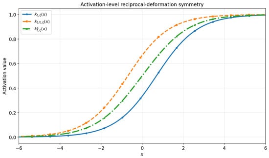
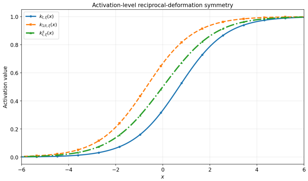
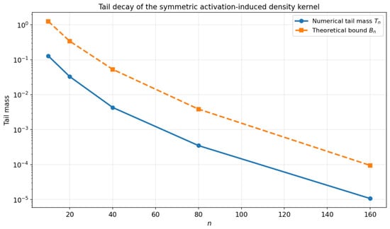
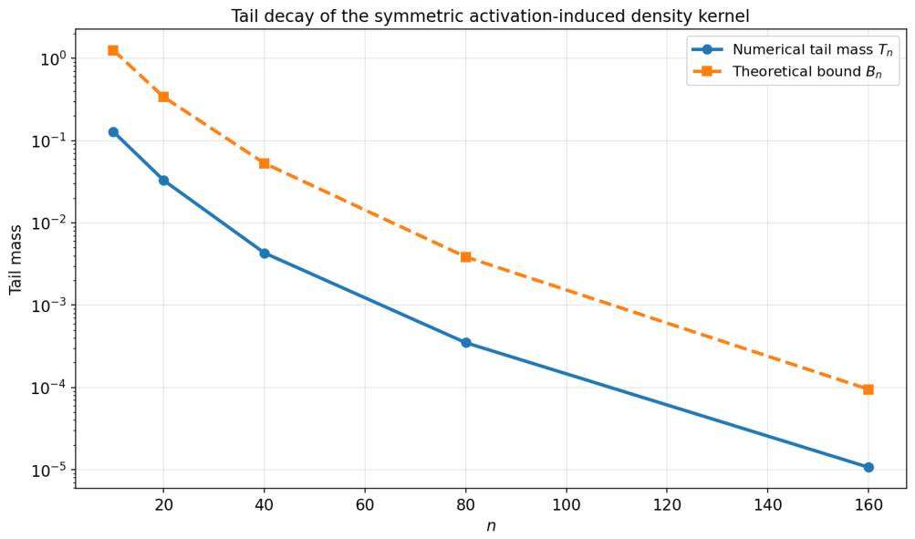
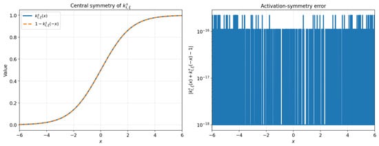
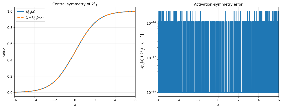
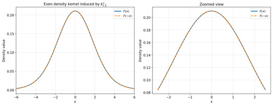
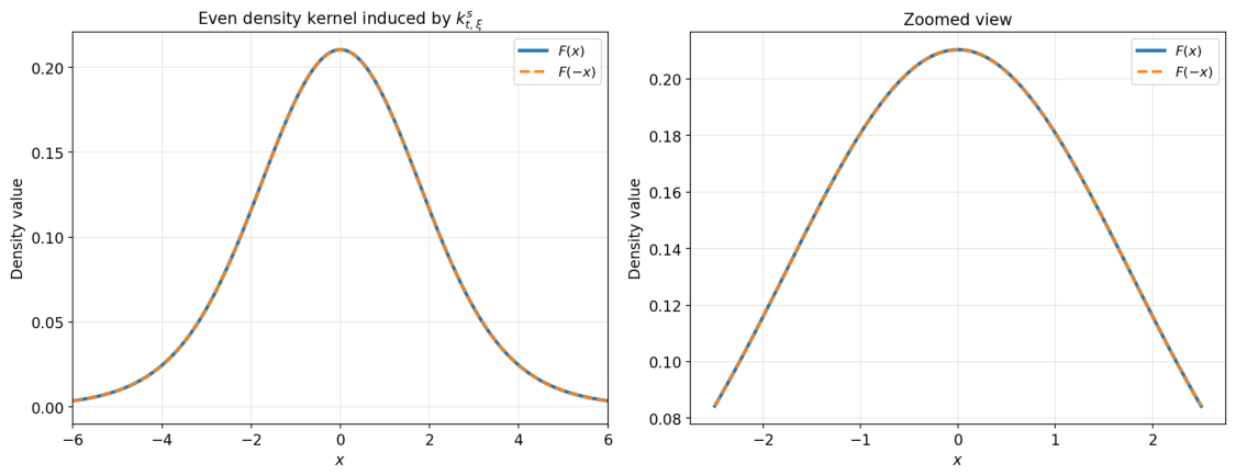
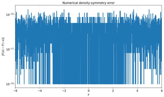
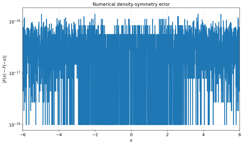
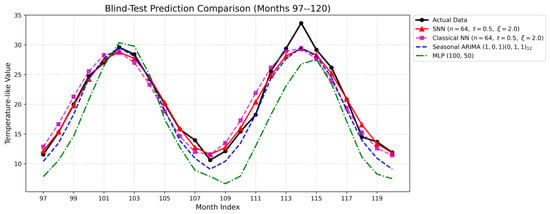
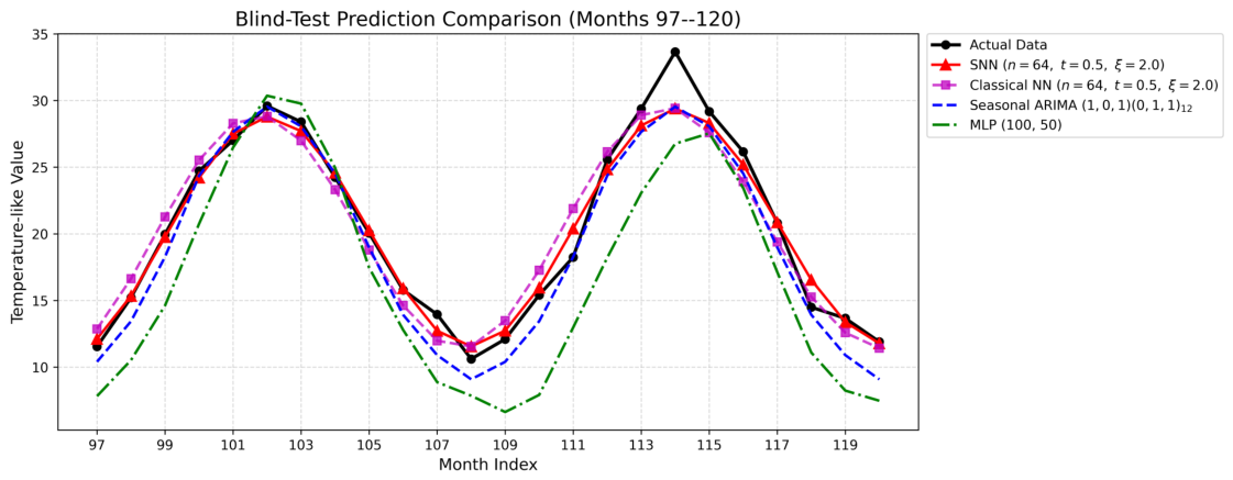
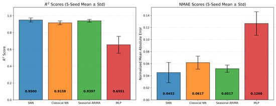
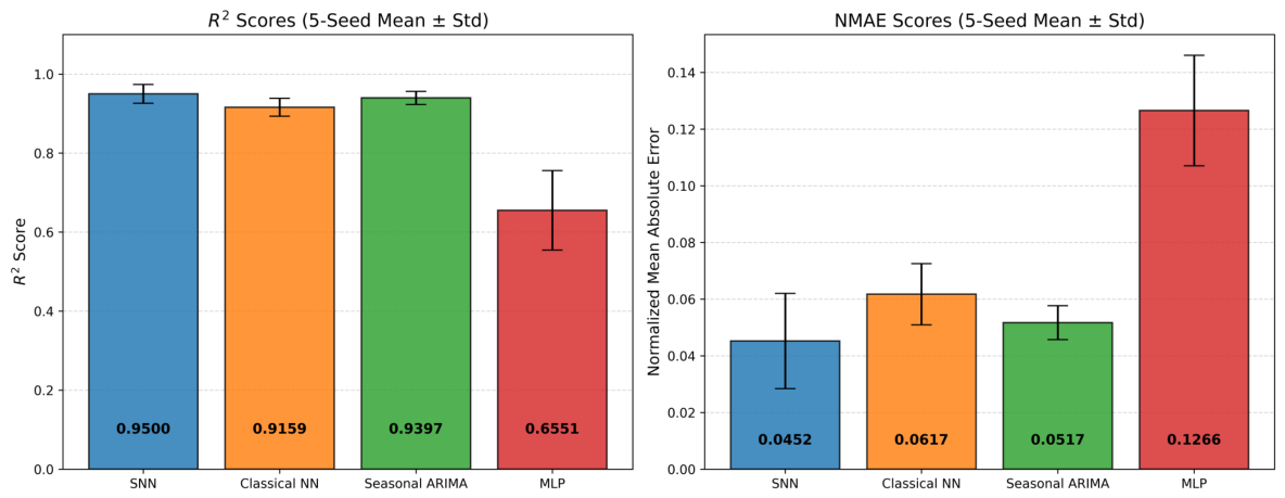
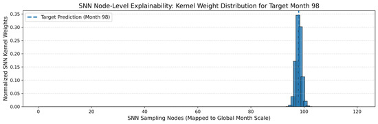
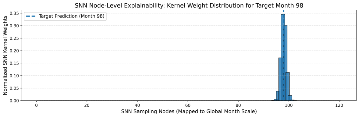
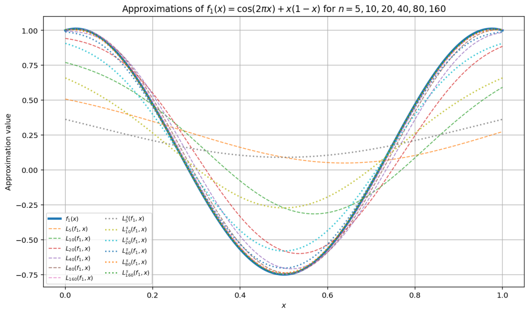
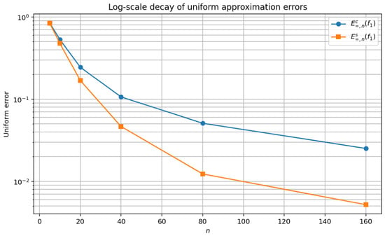
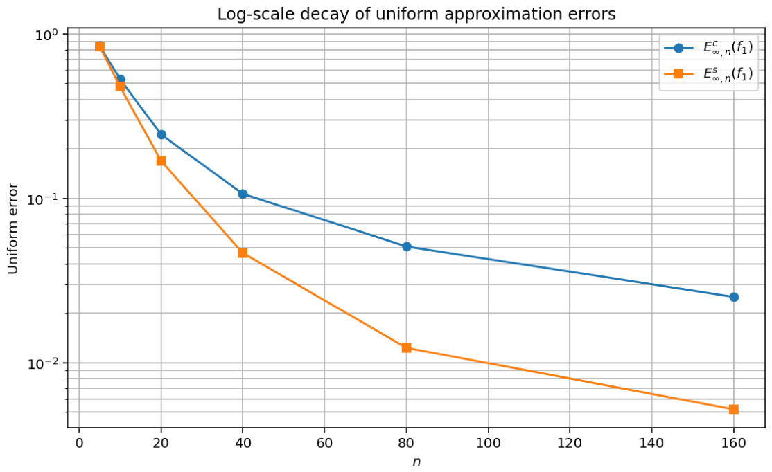
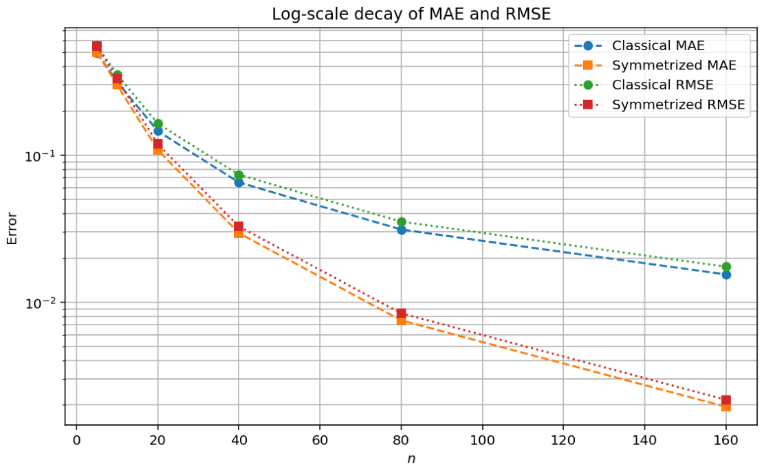
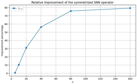
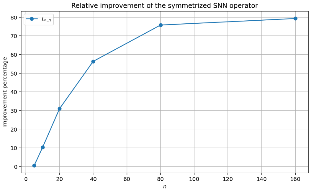
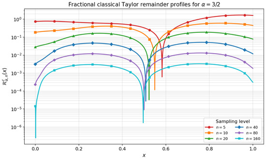
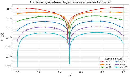
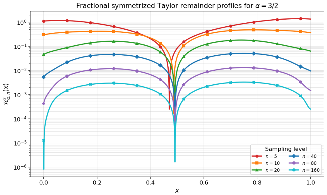
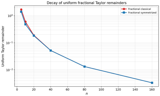
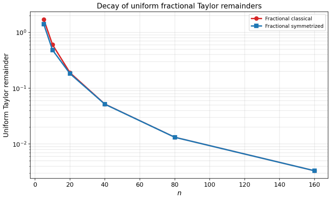
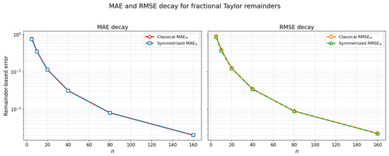
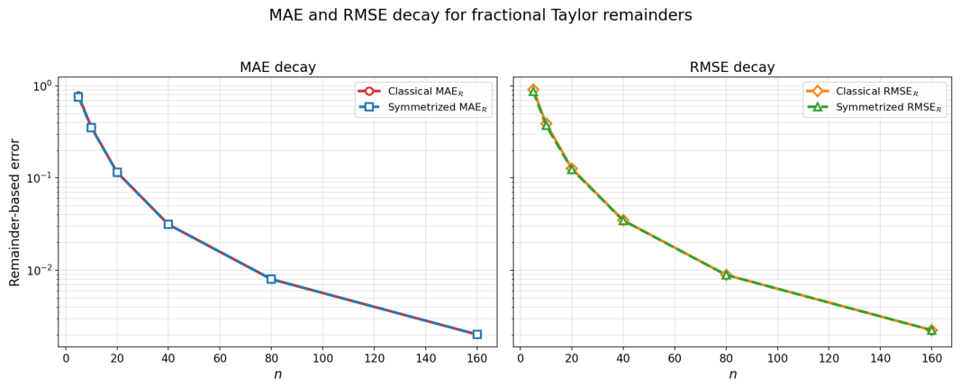
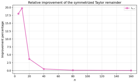
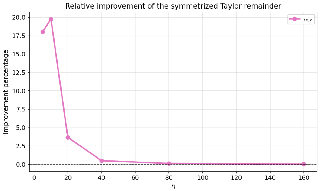
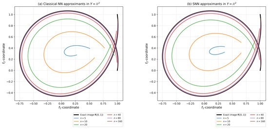
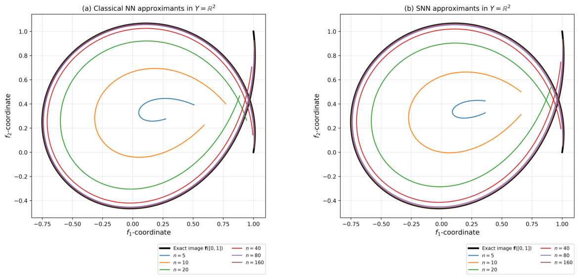

Disclaimer/Publisher’s Note: The statements, opinions and data contained in all publications are solely those of the individual author(s) and contributor(s) and not of MDPI and/or the editor(s). MDPI and/or the editor(s) disclaim responsibility for any injury to people or property resulting from any ideas, methods, instructions or products referred to in the content. |
© 2026 by the authors. Licensee MDPI, Basel, Switzerland. This article is an open access article distributed under the terms and conditions of the Creative Commons Attribution (CC BY) license.