Trajectory Tracking Control of an Off-Axis Tractor-Trailer Wheeled Mobile System with Passive Steering

Abstract

This paper investigates the system modeling and trajectory tracking control problem of an off-axis tractor-trailer wheeled mobile system and proposes a control strategy based on an integral sliding surface and a super-twisting algorithm. First, the motion relationship between the tractor and trailer is derived based on their geometric configuration, and the kinematic and dynamic models of the off-axis tractor-trailer wheeled mobile system with a passive steering angle are established. Then, a composite controller is designed by integrating the integral sliding surface with the super-twisting algorithm to achieve accurate tracking of the desired trajectory. During the controller design process, the desired trajectory is reconstructed as a curvature-consistent dynamic tracking target. Under this dynamic tracking target, the curvature deviation depends only on the yaw-rate error and is decoupled from longitudinal velocity disturbances, thereby improving trajectory tracking accuracy. Finally, numerical simulations are conducted to validate the effectiveness and generality of the proposed control strategy under three typical reference trajectories, including cycloidal, S-shaped, and circular trajectories. Comparisons with PID and feedback linearization control methods are also performed. The simulation results demonstrate that the off-axis tractor-trailer wheeled mobile system can closely follow the desired trajectories and exhibits satisfactory robustness.

1. Introduction

Off-axle tractor–trailer wheeled mobile systems consist of an actively driven tractor and one or more passive trailers connected through off-axle hitching mechanisms. Owing to their high payload capacity and operational flexibility, such systems have been widely employed in agricultural production, logistics transportation, and industrial material handling [1,2]. Compared with a single mobile platform, a tractor–trailer configuration connects the tractor and one or more passive trailers through articulated joints, thereby substantially enhancing transportation capacity and operational efficiency [3]. However, the inherent nonholonomic constraints, strong coupling, nonlinear dynamics, and underactuated characteristics of the system make accurate trajectory tracking a long-standing challenge in the field of mobile robotics [4,5].

According to the hitching configuration between the tractor and the trailer, tractor–trailer wheeled mobile systems can be classified into two fundamental architectures: on-axle and off-axle configurations [6]. In the on-axle configuration, the articulation point is located at the center of the rear axle of the leading vehicle, whereas in the off-axle configuration, the articulation point is displaced by a certain distance from the rear axle. Although the on-axle configuration can be regarded as a special case of the off-axle configuration, the two exhibit fundamentally different control characteristics [7]. Specifically, the introduction of an off-axle hitch destroys the differential flatness of the kinematic model, making exact feedback linearization inapplicable [8]. This significantly increases the complexity of controller design. Consequently, trajectory tracking control for off-axle tractor–trailer wheeled mobile systems is considerably more challenging while also being of greater practical significance.

A variety of control strategies have been developed for trajectory tracking of tractor–trailer wheeled mobile systems. For on-axle configurations, chain-transformation-based methods have been widely adopted for trajectory tracking of N-trailer systems. However, these methods are difficult to extend to off-axle systems. For off-axle systems, Michałek proposed a highly scalable cascade trajectory-tracking controller by introducing the concept of a formation-segment reference path, enabling asymptotic path tracking for an arbitrary number of off-axle trailers without requiring the computation of the shortest distance to the reference path [9]. Subsequently, Michałek further integrated the vector-field-oriented control approach with the cascade architecture and established a unified control framework for nonstandard N-trailer systems, capable of handling both point stabilization and trajectory-tracking tasks [7]. Ljungqvist proposed a lattice-based motion planning and trajectory-tracking framework for general two-trailer systems and developed a model predictive trajectory-tracking controller to address articulation-angle instability during reversing maneuvers [10]. Khalaji and Moosavian designed a robust adaptive controller for tractor–trailer wheeled mobile systems to cope with system nonlinearities and nonholonomic constraints and subsequently extended their work by incorporating the effects of wheel slip [11,12]. Leng and Minor proposed a curvature-based trajectory-tracking method for off-axle trailer systems. By integrating an active speed-limiting strategy with an extended Kalman filter-based sideslip estimator, the proposed method effectively improved tracking accuracy and robustness along variable-curvature paths [13]. Zhao developed a two-layer feedback control law for N-trailer systems by transforming the curvature-tracking problem into an articulation-angle stabilization problem, thereby achieving asymptotic stability within a cascade control framework [6]. Despite these advances, most existing approaches treat the trailer as a purely passive unit without steering capability. Consequently, the trailer trajectory inevitably deviates from that of the tractor, and this off-tracking effect becomes particularly pronounced for off-axle trailer systems during turning maneuvers.

To overcome the aforementioned limitation, the concept of passive steering was introduced. Reference [14] was the first to incorporate the passive steering angle into the kinematic modeling of tractor–trailer wheeled mobile systems. By employing a gear-based steering mechanism, the trailer was endowed with passive steering capability, enabling it to closely follow the trajectory of the tractor. On this basis, both the kinematic and dynamic models incorporating the passive steering angle were established. The original motion control problem was then reformulated as a curvature-tracking problem, and precise trajectory tracking was achieved using feedback linearization combined with optimal control. Subsequently, the passive steering strategy was extended to off-axle tractor–trailer wheeled mobile robots in [15], where a same-path trajectory-tracking control strategy was proposed, allowing both the tractor and the trailer to accurately follow the same geometric path. More recently, building upon these studies, the authors of [16] conducted the first systematic investigation of the motion characteristics of tractor systems with multiple trailers equipped with multiple passive steering angles. By integrating feedback linearization, optimal control, and integral sliding mode control, a driving torque controller was developed to achieve accurate tracking of a common reference path by the tractor and all trailers. These studies demonstrate that the introduction of passive steering provides an effective solution to the same-path trajectory-tracking problem for off-axle multi-trailer systems. Despite these advances, several limitations remain. First, existing trajectory-tracking methods generally rely on static reference velocity profiles, in which both the longitudinal and steering velocities are prescribed as time-dependent functions and remain independent of the actual motion states of the system. Second, the robustness of conventional controllers under complex disturbances remains limited. In particular, when model uncertainties and external disturbances coexist, conventional feedback linearization methods often fail to maintain satisfactory tracking performance. Third, a systematic quantitative comparison between dynamic and static reference trajectories is still lacking, making it difficult to fully assess the advantages of dynamic feedforward strategies. Owing to its inherent robustness against system uncertainties and external disturbances, sliding mode control has been widely applied to trajectory tracking of wheeled mobile systems [17]. Among various sliding mode techniques, the super-twisting algorithm, as a representative second-order sliding mode control method, effectively suppresses chattering while preserving the robustness of conventional sliding mode control. Furthermore, combining an integral sliding surface with the super-twisting algorithm can eliminate steady-state errors and further improve transient response performance [18].

Although the above studies have achieved considerable progress in trajectory tracking of tractor-trailer systems, several limitations still remain. First, most existing approaches employ static tracking targets, where the desired longitudinal velocity and yaw rate are predefined open-loop explicit functions independent of the current system states. Under varying-speed motion or external disturbances, once the actual system states deviate from the predefined targets, the tracking objectives cannot be adjusted accordingly, which may introduce additional curvature mismatch. Second, few studies have analytically investigated the structural difference in curvature deviation between dynamic and static trajectories. Therefore, the underlying reason why dynamic trajectory tracking strategies can improve tracking performance has not been sufficiently explained from a theoretical perspective. Third, although passive steering mechanisms have been introduced to enhance trajectory coordination between the tractor and trailer, most existing studies are still developed based on static tracking targets and do not fully exploit the potential advantages of combining passive steering mechanisms with dynamic reference strategies.

To address these issues, this paper proposes a curvature-consistent dynamic tracking target generation method and integrates it with a passive steering mechanism for trajectory tracking control of an off-axis tractor-trailer wheeled mobile system. By coupling the desired yaw rate with the actual longitudinal velocity according to the curvature of the desired trajectory, the proposed method enables curvature-consistent tracking of the desired path. Moreover, the structural difference in curvature deviation between dynamic and static tracking targets is analytically investigated, providing a theoretical explanation for the improved tracking performance achieved by the dynamic tracking strategy. The main contributions of this paper are summarized as follows:

(i) The relationship between the motion velocities of the tractor and trailer is derived through a geometric approach. A kinematic model of the off-axis tractor-trailer wheeled mobile system with a passive steering angle is established, together with the corresponding dynamic model, providing the basis for controller design.

(ii) A curvature-consistent dynamic tracking target generation method is proposed, and a trajectory tracking controller is designed by combining an integral sliding surface with a super-twisting algorithm. Theoretical analysis shows that, under the dynamic tracking target, $\mathsf{\Delta }k=e_{\omega }/v,$ the curvature deviation depends only on the yaw-rate tracking error and is decoupled from longitudinal velocity disturbances. In contrast, the static tracking target contains an additional curvature mismatch term. This analytical result reveals the theoretical reason why the dynamic tracking target improves trajectory tracking performance.

(iii) Taking the cycloidal trajectory as the primary reference path, together with additional S-shaped and circular trajectories, the performance differences between dynamic and static tracking strategies are quantitatively evaluated under different motion conditions. The evaluation is conducted in terms of longitudinal velocity error, yaw-rate error, and trajectory tracking error. Comparisons with PID and feedback linearization methods are further performed to assess the effectiveness and robustness of the proposed control strategy.

The remainder of this paper is organized as follows. First, the preliminaries are presented, and the system model of the off-axis tractor–trailer wheeled mobile system is established. Section 5 develops the proposed trajectory-tracking control strategy. Simulation studies are reported in Section 6 to validate the effectiveness of the proposed method. Finally, Section 7 concludes the paper.

2. Passive Steering Angle

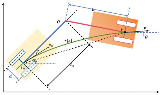
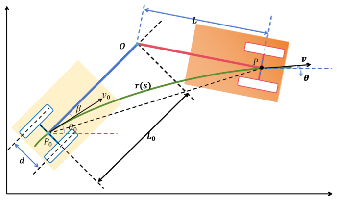
As illustrated in Figure 1, the off-axle tractor-trailer wheeled mobile system consists of a differentially driven two-wheeled tractor and a passive trailer. Let $P(x,y)$ and $P_0(x_0,y_0)$ denote the midpoints of the two parallel wheels of the tractor and the trailer, respectively. The tractor and the trailer are connected through an articulated linkage with corresponding link lengths L and $L_0$. The articulation point O is assumed to be a rigid joint, such that the two links undergo neither relative sliding nor length variation. The variables v and $v_0$ denote the longitudinal velocities of the tractor and the trailer, respectively. All wheels have an identical radius r, and the distance between the left and right wheels is d for both the tractor and the trailer. The variables $\theta$ and ${\theta }_0$ represent the heading angles of the tractor and the trailer, respectively, while $\beta$ denotes the passive steering angle of the trailer. Furthermore, ${\theta }_{l0}$, ${\theta }_{r0}$, ${\theta }_r$, and ${\theta }_l$ represent the rotational angles of the left and right wheels of the tractor and the trailer, respectively. Finally, $\phi =\theta -{\theta }_0$ denotes the relative heading angle between the tractor and the trailer.

To enable the tractor and the trailer to follow the same trajectory, this paper aims to design the passive steering angle of the trailer together with two wheel torque controllers for the tractor. To this end, according to the characteristics of the off-axle tractor-trailer wheeled mobile system, it is assumed that the vehicle operates at low speed and that all wheels satisfy the pure rolling condition without lateral slip. As shown in Figure 1, let $\mathbf{r}\left(s\right)=\left(x\left(s\right),y\left(s\right)\right),{\mathbf{r}}_0\left(s\right)=\left(x_0\left(s\right),y_0\left(s\right)\right)$ denote the position vectors of the tractor and the trailer, respectively. According to the geometric distance constraint, it follows that

$$∥\mathbf{r}\left(s\right)-{\mathbf{r}}_0\left(s\right)∥=\sqrt{L^2+L_0^2+2L{L}_0\cos \beta }.$$

(1)

When the off-axle tractor-trailer wheeled mobile system moves along the desired trajectory, the passive steering angle $\beta$ can be determined in advance from (1) together with the tangent direction of the reference path. In this case, however, $\beta$ remains a fixed steering angle. Under ideal conditions, both the tractor and the trailer can accurately follow the desired path. In practice, however, once small deviations arise between the actual and desired trajectories, a fixed steering angle cannot be adjusted online to compensate for the tracking errors, which may lead to error accumulation over time.

To overcome this limitation, the passive steering angle is designed as

$$\beta =\eta \left(s\right)\left(\theta -{\theta }_0\right)=\eta \left(s\right)\phi ,$$

(2)

where $\eta \left(s\right)$ is the steering gain associated with the local path curvature and the system parameters. Although the proposed steering angle remains a function of the arc length, it offers greater flexibility than the fixed steering angle obtained from (1). By adjusting the steering angle online according to the relative heading angle, the proposed strategy enables real-time compensation for trajectory deviations and provides a theoretical foundation for the subsequent trajectory-tracking controller design.

3. Kinematic Model

Let the generalized coordinates of the off-axle tractor-trailer wheeled mobile system be $\mathit{q}={\left(x,y,\theta ,\phi ,{\theta }_l,{\theta }_r\right)}^{\mathrm{T}},$ and let the state variables ${\left(x_0,y_0,{\theta }_0,{\theta }_{l0},{\theta }_{r0}\right)}^T$ be determined by the kinematic constraints of the system. The constraint equations can therefore be expressed in terms of $(\mathit{q},\dot{\mathit{q}})$.

The tractor is driven by two independently actuated wheels mounted on its left and right sides, whose driving torques generate the motion of the tractor and consequently propel the trailer. Under the assumption of pure rolling without lateral slip, the point $P(x,y)$ follows a smooth planar trajectory. Accordingly, the motion of the system satisfies the following nonholonomic constraint:

$$-\dot{x}\sin \theta +\dot{y}\cos \theta =0.$$

(3)

If point P possesses a nonzero lateral velocity at any instant, the resulting trajectory will contain a cusp and therefore cease to be smooth. Consequently, (3) is a necessary condition for the trajectory of point P to remain smooth.

Suppose that the trajectory of point P is the smooth planar curve $\mathbf{r}\left(t\right)=\left(x\left(t\right),y\left(t\right)\right),$ whose tangent vector has magnitude

$$v=\sqrt{{\dot{x}}^2+{\dot{y}}^2}.$$

(4)

Combining (3) and (4) yields

$$\left\{\begin{array}{c}-\dot{x}\sin \theta +\dot{y}\cos \theta =0,\hfill \\ v=\dot{x}\cos \theta +\dot{y}\sin \theta .\hfill \end{array}\right.$$

(5)

Equation (5) indicates that, for a smooth trajectory, the lateral velocity perpendicular to the tangent direction is identically zero, while the tangential velocity is equal to the longitudinal velocity along the trajectory. Therefore, (5) can be equivalently rewritten as

$$\left\{\begin{array}{cc}\hfill \dot{x}& =v\cos \theta ,\hfill \\ \hfill \dot{y}& =v\sin \theta .\hfill \end{array}\right.$$

(6)

Assuming pure rolling without slipping or wheel spin, the left and right driving wheels of the tractor satisfy

$$\left\{\begin{array}{cc}\hfill v& ={\displaystyle \frac{r}{2}}\left({\dot{\theta }}_r+{\dot{\theta }}_l\right),\hfill \\ \hfill \dot{\theta }& ={\displaystyle \frac{r}{d}}\left({\dot{\theta }}_r-{\dot{\theta }}_l\right).\hfill \end{array}\right.$$

(7)

In summary, throughout its motion, the tractor is subject to one nonholonomic constraint, given by (3), and two holonomic constraints described by (7). Solving (7) for ${\dot{\theta }}_r$ and ${\dot{\theta }}_l$ and combining the resulting expressions with (6) yields the following constraint equations:

$$\left\{\begin{array}{c}\dot{x}=v\cos \theta ,\hfill \\ \dot{y}=v\sin \theta ,\hfill \\ {\dot{\theta }}_r={\displaystyle \frac{1}{r}}v+{\displaystyle \frac{d}{2r}}\dot{\theta },\hfill \\ {\dot{\theta }}_l={\displaystyle \frac{1}{r}}v-{\displaystyle \frac{d}{2r}}\dot{\theta }.\hfill \end{array}\right.$$

(8)

Substituting the second equation of (7) into the last two equations of (8), together with the nonholonomic constraint (3), the motion constraints can be equivalently expressed as

$$\left\{\begin{array}{c}-\dot{x}\sin \theta +\dot{y}\cos \theta =0,\hfill \\ \dot{x}\cos \theta +\dot{y}\sin \theta +{\displaystyle \frac{d}{2}}\dot{\theta }-r{\dot{\theta }}_r=0,\hfill \\ \dot{x}\cos \theta +\dot{y}\sin \theta -{\displaystyle \frac{d}{2}}\dot{\theta }-r{\dot{\theta }}_l=0.\hfill \end{array}\right.$$

(9)

By analyzing the kinematic relationship between the tractor and the trailer at the articulation point O shown in Figure 1, the following equations can be obtained:

$$\left\{\begin{array}{cc}\hfill v\cos \theta +L\dot{\theta }\sin \theta & =v_0\cos ({\theta }_0+\beta )-L_0{\dot{\theta }}_0\sin {\theta }_0,\hfill \\ \hfill v\sin \theta -L\dot{\theta }\cos \theta & =v_0\sin ({\theta }_0+\beta )+L_0{\dot{\theta }}_0\cos {\theta }_0.\hfill \end{array}\right.$$

(10)

After straightforward manipulation of (10), one obtains

$$\left\{\begin{array}{cc}\hfill v& =v_0\cos (\beta -\phi )-L_0{\dot{\theta }}_0\sin \phi ,\hfill \\ \hfill L\dot{\theta }& =-v_0\sin (\beta -\phi )-L_0{\dot{\theta }}_0\cos \phi .\hfill \end{array}\right.$$

(11)

Further eliminating ${\dot{\theta }}_0$ from (11) gives the trailer velocity

$$v_0\cos \beta =v\cos \phi -L\dot{\theta }\sin \phi .$$

(12)

Using the differential relationship of the relative heading angle, (12) can be rewritten as

$$\dot{\phi }={\displaystyle \frac{\sin (\beta -\phi )}{L_0\cos \beta }}v+\left(1+{\displaystyle \frac{L\cos (\beta -\phi )}{L_0\cos \beta }}\right)\dot{\theta }.$$

(13)

Accordingly, all the constraint equations of the off-axle tractor-trailer wheeled mobile system can be summarized as

$$\left\{\begin{array}{c}-\dot{x}\sin \theta +\dot{y}\cos \theta =0,\hfill \\ \dot{x}\cos \theta +\dot{y}\sin \theta +{\displaystyle \frac{d}{2}}\dot{\theta }-r{\dot{\theta }}_r=0,\hfill \\ \dot{x}\cos \theta +\dot{y}\sin \theta -{\displaystyle \frac{d}{2}}\dot{\theta }-r{\dot{\theta }}_l=0,\hfill \\ \dot{x}\cos \theta \sin (\beta -\phi )+\dot{y}\sin \theta \sin \phi (\beta -\phi )+\left(L_0\cos \beta +L\cos (\phi +\beta )\right)\dot{\theta }-L_0\cos \beta \dot{\phi }=0.\hfill \end{array}\right.$$

(14)

Equation (14) can be compactly written in matrix form as

$$\mathit{F}{\left(\mathit{q}\right)}_{4\times 6}{\dot{\mathit{q}}}_{6\times 1}={\mathbf{0}}_{4\times 1},$$

(15)

where

$$\mathit{F}\left(\mathit{q}\right)=\left[\begin{array}{cccccc}-\sin \theta & \cos \theta & 0& 0& 0& 0\\ \cos \theta & \sin \theta & {\displaystyle \frac{d}{2}}& 0& -r& 0\\ \cos \theta & \sin \theta & -{\displaystyle \frac{d}{2}}& 0& 0& -r\\ \cos \theta \sin (\beta -\phi )& \sin \theta \sin (\beta -\phi )& L_0\cos \beta +L\cos (\beta -\phi )& -L_0\cos \beta & 0& 0\end{array}\right].$$

Combining (9) and (13), the complete set of constraint equations for the off-axle tractor-trailer wheeled mobile system can be written as

$$\left\{\begin{array}{cc}\hfill \dot{x}& =v\cos \theta ,\hfill \\ \hfill \dot{y}& =v\sin \theta ,\hfill \\ \hfill \dot{\theta }& =\dot{\theta },\hfill \\ \hfill \dot{\phi }& ={\displaystyle \frac{\sin (\beta -\phi )}{L_0\cos \beta }}v+\left(1+{\displaystyle \frac{L\cos (\beta -\phi )}{L_0\cos \beta }}\right)\dot{\theta },\hfill \\ \hfill {\dot{\theta }}_r& ={\displaystyle \frac{1}{r}}v+{\displaystyle \frac{d}{2r}}\dot{\theta },\hfill \\ \hfill {\dot{\theta }}_l& ={\displaystyle \frac{1}{r}}v-{\displaystyle \frac{d}{2r}}\dot{\theta }.\hfill \end{array}\right.$$

(16)

Equation (16) can be expressed in the following matrix form:

$${\dot{\mathit{q}}}_{6\times 1}=\mathit{S}{\left(\mathit{q}\right)}_{6\times 2}{\mathit{V}}_{2\times 1},$$

(17)

where

$$\mathit{S}\left(\mathit{q}\right)=\left[\begin{array}{cc}\cos \theta & 0\\ \sin \theta & 0\\ 0& 1\\ {\displaystyle \frac{\sin (\beta -\phi )}{L_0\cos \beta }}& \left(1+{\displaystyle \frac{L\cos (\beta -\phi )}{L_0\cos \beta }}\right)\\ {\displaystyle \frac{1}{r}}& {\displaystyle \frac{d}{2r}}\\ {\displaystyle \frac{1}{r}}& -{\displaystyle \frac{d}{2r}}\end{array}\right],\mathit{V}=\left[\begin{array}{c}v\\ \dot{\theta }\end{array}\right].$$

From (15) and (17), it is straightforward to verify that

$$\mathit{F}{\left(\mathit{q}\right)}_{4\times 6}{\mathit{S}}_{6\times 2}={\mathbf{0}}_{4\times 2}.$$

(18)

Remark 1. 

Compared with the standard tractor-trailer kinematic model, the modifications introduced in this paper mainly lie in three aspects. First, by introducing the passive steering angle $\beta =\eta \left(s\right)\phi$, the trailer is endowed with the capability of passively following the tractor trajectory without requiring additional actuators or sensors on the trailer. Second, the kinematic equations are systematically derived for the off-axis articulated structure. Since the articulation point is offset from the center of the rear axle, the differential flatness property is lost, and feedback linearization methods cannot be directly applied. Therefore, the kinematic modeling of the off-axis structure is more involved than that of conventional tractor-trailer systems.

4. Dynamic Model

The dynamic model of the off-axle tractor-trailer wheeled mobile system is derived using the Euler–Lagrange formulation for nonholonomic mechanical systems. The equations of motion are given by

$${\displaystyle \frac{d}{dt}}\left({\displaystyle \frac{\partial L}{\partial \dot{\mathit{q}}}}\right)-{\displaystyle \frac{\partial L}{\partial \mathit{q}}}=\mathit{E}\left(\mathit{q}\right)\mathit{T}+{\mathit{F}}^{\mathrm{T}}\left(\mathit{q}\right)\lambda ,$$

(19)

where

$$\mathit{T}=\left[\begin{array}{c}{T}_r\\ T_l\end{array}\right],\mathit{E}\left(\mathit{q}\right)={\left[\begin{array}{cccccc}0& 0& 0& 0& 1& 0\\ 0& 0& 0& 0& 0& 1\end{array}\right]}^{\mathrm{T}}.$$

Here, $\lambda$ denotes the vector of Lagrange multipliers, $\mathit{T}$ is the input torque vector, $\mathit{E}\left(\mathit{q}\right)$ is the input distribution matrix, and $T_r$ and $T_l$ represent the driving torques applied to the right and left wheels of the tractor, respectively.

The kinetic energy of each component of the off-axle tractor-trailer wheeled mobile system is derived next. The kinetic energy of the tractor consists of the translational kinetic energy, the rotational kinetic energy of the vehicle body, and the rotational kinetic energy of the two driving wheels, which can be written as

$$T_f={\displaystyle \frac{1}{2}}{M}_f({\dot{x}}^2+{\dot{y}}^2)+\left(I_{wd}+{\displaystyle \frac{1}{2}}{I}_{fd}\right){\dot{\theta }}^2+{\displaystyle \frac{1}{2}}\left(I_w+M_w{r}^2\right)\left({\dot{\theta }}_r^2+{\dot{\theta }}_l^2\right).$$

Similarly, the forward kinetic energy and rotational kinetic energy of the intermediate body and the trailer in the off-axle tractor-trailer wheeled mobile system are respectively given by

$$\begin{array}{cc}\hfill T_c=& {\displaystyle \frac{1}{2}}(M_{C_1}+M_{C_2})({\dot{x}}^2+{\dot{y}}^2)-M_{C_2}L\dot{\theta }(\dot{x}\sin \theta -\dot{y}\cos \theta )\hfill \\ \hfill & -{\displaystyle \frac{1}{2}}{M}_{C_2}{L}_0(\dot{\theta }-\dot{\phi })\left(\dot{x}\sin (\theta -\phi )-\dot{y}\cos (\theta -\phi )\right)\hfill \\ \hfill & -{\displaystyle \frac{1}{2}}{M}_{C_2}L{L}_0\dot{\theta }(\dot{\theta }-\dot{\phi })\cos \phi +{\displaystyle \frac{1}{2}}{I}_{C_1}{\dot{\theta }}^2+{\displaystyle \frac{1}{2}}{I}_{C_2}{(\dot{\theta }-\dot{\phi })}^2,\hfill \end{array}$$

and

$$\begin{array}{cc}\hfill T_g=& {\displaystyle \frac{1}{2}}{M}_r({\dot{x}}^2+{\dot{y}}^2)-M_{r}L\dot{\theta }(\dot{x}\sin \theta -\dot{y}\cos \theta )+M_r{L}_0(\dot{\theta }-\dot{\phi })\left(\dot{x}\sin (\theta -\phi )-\dot{y}\cos (\theta -\phi )\right)\hfill \\ \hfill & +{\displaystyle \frac{1}{2}}(M_r{L}^2+I_{rd}){\dot{\theta }}^2+{\displaystyle \frac{1}{8}}\left(4M_r{L}_0^2+4I_{rd}+{\displaystyle \frac{I_w{d}^2}{r^2}}+M_w{d}^2\right){(\dot{\theta }-\dot{\phi })}^2\hfill \\ \hfill & -M_{r}L{L}_0\dot{\theta }(\dot{\theta }-\dot{\phi })\cos \phi +{\displaystyle \frac{I_w+M_w{r}^2}{4}}{\left[({\dot{\theta }}_l+{\dot{\theta }}_r)\cos \phi -{\displaystyle \frac{2L}{d}}({\dot{\theta }}_r-{\dot{\theta }}_l)\sin \phi \right]}^2.\hfill \end{array}$$

Here, $M_w$ denotes the mass of each wheel; $M_f$ and $M_r$ are the masses of the tractor and the trailer excluding the wheels, respectively; $M_{C_1}$ and $M_{C_2}$ denote the masses of the connecting rod attached to the tractor and the trailer at point C, respectively. Moreover, $I_{wd}$, $I_{fd}$, and $I_{rd}$ represent the moments of inertia of the wheel, tractor, and trailer about the z-axis, respectively, while $I_{C_1}$, $I_{C_2}$, and $I_w$ denote the moments of inertia of the connecting rod and the wheel about the wheel axis.

Substituting the Lagrangian $L=T_f+T_c+T_g$ into Equation (19), together with the geometric relationships among the system components, and arranging the resulting expressions according to the generalized coordinates yield

$$\mathit{A}\left(\mathit{q}\right)\ddot{\mathit{q}}+\mathit{U}(\mathit{q},\dot{\mathit{q}})=\mathit{E}\left(\mathit{q}\right)\mathit{T}+{\mathit{F}}^{\mathit{T}}\left(\mathit{q}\right)\lambda ,$$

(20)

where

$$\mathit{A}\left(\mathit{q}\right)=\left[\begin{array}{cccccc}{a}_{11}& 0& a_{13}& a_{14}& 0& 0\\ 0& a_{22}& a_{23}& a_{24}& 0& 0\\ a_{31}& a_{32}& a_{33}& a_{34}& 0& 0\\ a_{41}& a_{42}& a_{43}& a_{44}& 0& 0\\ 0& 0& 0& 0& a_{55}& a_{56}\\ 0& 0& 0& 0& a_{65}& a_{66}\end{array}\right],\mathit{U}(\mathit{q},\dot{\mathit{q}})=\left[\begin{array}{c}{u}_1\\ u_2\\ u_3\\ u_4\\ u_5\\ u_6\end{array}\right].$$

Differentiating both sides of Equation (17) with respect to time and substituting the result into Equation (20) gives

$$\mathit{A}\left(\mathit{q}\right)\dot{\mathit{S}}\left(\mathit{q}\right)\mathit{V}+\mathit{A}\left(\mathit{q}\right)\mathit{S}\left(\mathit{q}\right)\dot{\mathit{V}}+\mathit{U}(\mathit{q},\dot{\mathit{q}})=\mathit{E}\left(\mathit{q}\right)\mathit{T}+{\mathit{F}}^{\mathit{T}}\left(\mathit{q}\right)\lambda .$$

Premultiplying both sides of the above equation by ${\mathit{S}}^{\mathrm{T}}\left(\mathit{q}\right)$ and using the orthogonality condition in Equation (18) to eliminate the Lagrange multiplier yield

$${\mathit{S}}^{\mathrm{T}}\left(\mathit{q}\right)\mathit{A}\left(\mathit{q}\right)\dot{\mathit{S}}\left(\mathit{q}\right)\mathit{V}+{\mathit{S}}^{\mathrm{T}}\left(\mathit{q}\right)\mathit{A}\left(\mathit{q}\right)\mathit{S}\left(\mathit{q}\right)\dot{\mathit{V}}+{\mathit{S}}^{\mathrm{T}}\left(\mathit{q}\right)\mathit{U}(\mathit{q},\dot{\mathit{q}})={\mathit{S}}^{\mathrm{T}}\left(\mathit{q}\right)\mathit{E}\left(\mathit{q}\right)\mathit{T}.$$

By rearranging the above equations, the dynamic model of the off-axle tractor-trailer wheeled mobile system can be expressed as

$$\left\{\begin{array}{cc}\hfill \dot{v}& ={\gamma }_{1}v+{\gamma }_2{u}_1+{\gamma }_3{u}_2+{\gamma }_4,\hfill \\ \hfill \dot{\omega }& =\ddot{\theta }={\beta }_{1}v+{\beta }_2{u}_1+{\beta }_3{u}_2+{\beta }_4.\hfill \end{array}\right.$$

(21)

where v and $\omega$ denote the forward velocity and yaw rate of the tractor, respectively.

The detailed derivation and the explicit expressions of the model parameters are provided in the Appendix A.

5. Motion Control Design

It follows from Equation (21) that the off-axle tractor-trailer wheeled mobile system takes ${\mu }_1$ and ${\mu }_2$ as the control inputs, while the forward velocity v and yaw rate $\dot{\theta }$ are selected as the controlled outputs. Therefore, the system can be regarded as a typical two-input two-output nonlinear system. Owing to the presence of nonlinear dynamic coupling, parameter uncertainties, and external disturbances, conventional control methods often fail to simultaneously achieve high tracking accuracy, rapid dynamic response, and strong disturbance rejection capability. To address these challenges, a composite sliding mode controller integrating an integral sliding mode surface and the super-twisting algorithm is developed. The integral sliding mode surface is employed to construct the sliding dynamics, where the introduction of the integral term eliminates steady-state tracking errors and ensures that the system trajectory starts on the sliding manifold from the initial instant, thereby effectively reducing the disturbance sensitivity during the reaching phase. Furthermore, a super-twisting control law is incorporated to provide finite-time compensation for lumped disturbances through a continuous control input, which fundamentally alleviates the high-frequency chattering phenomenon inherent in conventional sliding mode control. As a result, high-precision trajectory tracking can be achieved under dynamic operating conditions. The controller design procedure is detailed as follows.

Equation (21) can be rewritten in the following state-space form:

$$\dot{\mathit{z}}=\left[\begin{array}{c}\dot{v}\\ \dot{\omega }\end{array}\right]=\mathit{f}\left(\mathit{z}\right)+\mathit{g}\left(\mathit{z}\right)\mathit{u},$$

(22)

where

$$\mathit{f}\left(\mathit{z}\right)=\left[\begin{array}{c}{\gamma }_{1}v+{\gamma }_4\\ {\beta }_{1}v+{\beta }_4\end{array}\right],\mathit{g}\left(\mathit{z}\right)=\left[\begin{array}{cc}{\gamma }_2& {\gamma }_3\\ {\beta }_2& {\beta }_3\end{array}\right],\mathit{u}=\left[\begin{array}{c}{u}_1\\ u_2\end{array}\right].$$

Define the tracking error as $\mathit{e}={\left[\begin{array}{cc}{e}_v& e_{\theta }\end{array}\right]}^{\mathrm{T}}=\mathit{z}-{\mathit{z}}_d.$ To design a switching controller capable of handling various uncertainties, the following integral sliding mode surface is introduced:

$$S\left(\mathit{z}\left(t\right)\right)=\mathit{e}+\lambda {\int }_0^t\mathit{e}\left(\tau \right)\mathrm{d}\tau ,$$

where $\lambda =\mathrm{diag}({\lambda }_1,{\lambda }_2)>0$ is the sliding-surface parameter matrix, and $S={\left[\begin{array}{cc}{S}_1& S_2\end{array}\right]}^T$ denotes the sliding mode vector.

Taking the time derivative of the integral sliding surface yields

$$\dot{S}=\dot{\mathit{e}}+\lambda \mathit{e}=(\dot{\mathit{z}}-{\dot{\mathit{z}}}_d)+\lambda \mathit{e}.$$

(23)

Setting $\dot{S}=0$ gives

$$\mathbf{0}=\mathit{f}\left(\mathit{z}\right)+\mathit{g}\left(\mathit{z}\right)u_s-{\dot{\mathit{z}}}_d+\lambda \mathit{e},$$

(24)

from which the equivalent control law is obtained as

$$u_s={\mathit{g}}^{-1}\left(\mathit{z}\right)\left(-\lambda \mathit{e}+{\dot{\mathit{z}}}_d-\mathit{f}\left(\mathit{z}\right)\right).$$

(25)

Conventional sliding mode control employs a discontinuous sign function, which inevitably introduces high-frequency chattering into the control input. To alleviate this drawback, the super-twisting algorithm is incorporated to suppress chattering through an integral correction term while enhancing robustness against system uncertainties and external disturbances. Furthermore, to eliminate the discontinuity caused by the sign function, the following smooth approximation is adopted:

$$\mathrm{sgn}\left(S_i\right)\approx {\displaystyle \frac{S_i}{\epsilon +\left|S_i\right|}},\epsilon >0.$$

To further enhance the robustness of the controller against system uncertainties and external disturbances, the super-twisting control component is introduced as

$$u_x=-{\mathit{g}}^{-1}\left(\mathit{z}\right)u_{xx},$$

(26)

where $u_{xx}$ denotes the super-twisting control vector, defined as

$$u_{xx}=\left[\begin{array}{c}{\displaystyle k_{11}{\left|S_1\right|}^{\frac{1}{2}}{\displaystyle \frac{S_1}{\epsilon +|S_1|}}+{\int }_0^t{k}_{21}{\displaystyle \frac{S_1\left(\tau \right)}{\epsilon +|S_1\left(\tau \right)|}}d\tau }\\ {\displaystyle k_{12}{\left|S_2\right|}^{\frac{1}{2}}{\displaystyle \frac{S_2}{\epsilon +|S_2|}}+{\int }_0^t{k}_{22}{\displaystyle \frac{S_2\left(\tau \right)}{\epsilon +|S_2\left(\tau \right)|}}d\tau }\end{array}\right].$$

Accordingly, the overall control law is given by

$$\begin{array}{cc}\hfill u& =u_s+u_x\hfill \\ \hfill & ={\mathit{g}}^{-1}\left(z\right)\left(-\lambda \mathit{e}+{\dot{\mathit{z}}}_d-\mathit{f}\left(\mathit{z}\right)-\left[\begin{array}{c}{\displaystyle k_{11}{\left|S_1\right|}^{\frac{1}{2}}{\displaystyle \frac{S_1}{\epsilon +|S_1|}}+{\int }_0^t{k}_{21}{\displaystyle \frac{S_1\left(\tau \right)}{\epsilon +|S_1\left(\tau \right)|}}d\tau }\\ {\displaystyle k_{12}{\left|S_2\right|}^{\frac{1}{2}}{\displaystyle \frac{S_2}{\epsilon +|S_2|}}+{\int }_0^t{k}_{22}{\displaystyle \frac{S_2\left(\tau \right)}{\epsilon +|S_2\left(\tau \right)|}}d\tau }\end{array}\right]\right).\hfill \end{array}$$

(27)

Substituting the proposed controller into the system dynamics yields

$$\dot{S}=-u_{xx}+\mathsf{\Delta }\left(t\right),$$

where $\mathsf{\Delta }\left(t\right)$ denotes the lumped uncertainty of the system and satisfies $|{\mathsf{\Delta }}_i\left(t\right)|\le {\mathsf{\Delta }}_{i,\max }.$

Accordingly, the system dynamics in (22) can be rewritten as

$$\dot{\mathit{z}}=\mathit{f}\left(\mathit{z}\right)+\mathit{g}\left(\mathit{z}\right)u+\mathsf{\Delta }\left(t\right).$$

(28)

For each sliding surface component $S_i$, the controller parameters are selected to satisfy

$$k_{2i}>{\mathsf{\Delta }}_{i,\max },k_{1i}>\sqrt{{\displaystyle \frac{2}{k_{2i}-{\mathsf{\Delta }}_{i,\max }}}·{\displaystyle \frac{(k_{2i}+{\mathsf{\Delta }}_{i,\max })(1+p_i)}{1-p_i}}},$$

where $0<p_i<1.$ Then, the system states converge to the integral sliding surface $S=0$ within a finite time. Once the sliding motion is established, the tracking error dynamics satisfy $\dot{e}+\lambda e=0,$ which implies that the tracking error converges to zero exponentially.

6. Simulation Results

To comprehensively evaluate the effectiveness and robustness of the proposed control method, numerical simulations are conducted in this section using three typical reference trajectories, namely cycloidal, S-shaped, and circular trajectories. Furthermore, comparative studies with existing control methods are performed to assess the performance of the proposed approach. First, trajectory tracking simulations under the cycloidal reference trajectory are carried out, and the robustness of the proposed method is evaluated in the presence of parameter uncertainties and measurement noise. Then, under the same cycloidal trajectory and disturbance conditions, the proposed method is compared with existing control approaches to further demonstrate its tracking performance. Finally, tracking experiments with S-shaped and circular reference trajectories are conducted to verify the applicability and generality of the proposed method under trajectories with different curvature characteristics.

6.1. Tracking Performance and Robustness Analysis for a Cycloidal Trajectory

In this subsection, the tracking performance and robustness of the proposed control strategy are evaluated under a cycloidal reference trajectory. The off-axis tractor-trailer wheeled mobile system is initially assumed to be at rest. The desired trajectory is selected as a cycloidal curve, which is given by

$$\widehat{\mathbf{r}}\left(t\right)=\left(\widehat{x}\left(t\right),\widehat{y}\left(t\right)\right)=\left(t-\sin t,1-\cos t\right),t\in (0,2\pi ),$$

(29)

whose curvature is given by

$$k\left(t\right)=-{\displaystyle \frac{1}{4\sin \left({\displaystyle \frac{t}{2}}\right)}}.$$

Since the curvature of the cycloidal trajectory approaches infinity at its endpoints, directly employing it as the dynamic reference trajectory for trajectory tracking may lead to significant numerical errors during computation. Therefore, a segment of the cycloidal curve excluding the singular endpoints is selected as the desired reference trajectory:

$$\widehat{\mathbf{r}}\left(t\right)=\left(\widehat{x}\left(t\right),\widehat{y}\left(t\right)\right)=\left(t+{\displaystyle \frac{\pi }{4}}-\sin \left(t+{\displaystyle \frac{\pi }{4}}\right),1-\cos \left(t+{\displaystyle \frac{\pi }{4}}\right)\right),t\in \left[0,{\displaystyle \frac{3\pi }{2}}\right].$$

(30)

Meanwhile, the corresponding arc-length function is given by

$$s\left(t\right)={\int }_0^t\sqrt{2\sin \left({\displaystyle \frac{y}{2}}+{\displaystyle \frac{\pi }{8}}\right)}dy=4\cos {\displaystyle \frac{\pi }{8}}-4\cos {\displaystyle \frac{t+\pi /4}{2}}.$$

The total arc length of the reference trajectory is $l=s\left({\displaystyle \frac{3\pi }{2}}\right)=8\cos {\displaystyle \frac{\pi }{8}},$ and the curvature expressed as a function of the arc length is

$$k\left(s\right)=-{\displaystyle \frac{1}{\sqrt{16-16{\cos }^2\frac{\pi }{8}-s^2+8s\cos \frac{\pi }{8}}}}.$$

(31)

Accordingly, the desired steady-state trajectory of the tractor is specified as

$$\left\{\begin{array}{c}\widehat{v}=2\sin {\displaystyle \frac{t+\pi /4}{2}},\hfill \\ \widehat{\omega }=\dot{\widehat{\theta }}=-{\displaystyle \frac{1}{2}},\hfill \end{array}\right.t\in \left[0,{\displaystyle \frac{3\pi }{2}}\right].$$

(32)

In practical trajectory-tracking applications, if the objective is solely to ensure that the wheeled mobile robot accurately follows the prescribed geometric path without imposing constraints on its traveling speed, the dynamic reference trajectory can be designed as

$$\left\{\begin{array}{c}\tilde{\omega }=\dot{\tilde{\theta }}=k\left(s\right)\tilde{v},s\left(t\right)={\int }_0^{t}v\left(\tau \right)d\tau ,\hfill \\ \tilde{v}={\displaystyle \frac{\ddot{\tilde{x}}\dot{\tilde{y}}-\dot{\tilde{x}}\ddot{\tilde{y}}}{{\dot{\tilde{x}}}^2+{\dot{\tilde{y}}}^2}}\dot{\varphi }\left(t\right).\hfill \end{array}\right.$$

(33)

Let $\theta$ denote the actual forward velocity of the trailer, and let $k\left(s\right)$ denote the curvature of the trailer trajectory. The reference forward velocity is denoted by $\dot{\varphi }\left(t\right)$. The function $\varphi \left(t\right)$ is designed as $\dot{\varphi }\left(t\right)=l{\xi }^{2}t{e}^{-\xi t}.$ Accordingly, the corrected dynamic trajectory of the trailer is given by

$$\left\{\begin{array}{c}\tilde{v}=2\cos {\displaystyle \frac{\pi }{8}}t{e}^{-{\displaystyle \frac{1}{2}}t},\hfill \\ \ddot{\theta }=-{\displaystyle \frac{v}{\sqrt{16-16{\cos }^2\frac{\pi }{8}-s^2+8s\cos \frac{\pi }{8}}}},s\in \left[0,8\cos {\displaystyle \frac{\pi }{8}}\right].\hfill \end{array}\right.$$

(34)

For the trailer system, since ${\theta }_0=\theta -\phi$, combining Equation (11) yields the relationship between $(v,\dot{\theta })$ and $(v_0,{\dot{\theta }}_0)$ as

$$\left\{\begin{array}{c}{v}_0={\displaystyle \frac{v\cos \phi +L\dot{\theta }\sin \phi }{\cos \beta }},\hfill \\ {\dot{\theta }}_0=-{\displaystyle \frac{\sin (\beta -\phi )}{L_0\cos \beta }}v-{\displaystyle \frac{L\cos (\beta -\phi )}{L_0\cos \beta }}\dot{\theta }.\hfill \end{array}\right.$$

(35)

In the simulation, the parameters of the off-axis trailer-type mobile system are selected as follows:

$$\begin{array}{cc}\hfill & I_{fd}=0.03\mathrm{kg}·{\mathrm{m}}^2,I_{rd}=0.02\mathrm{kg}·{\mathrm{m}}^2,I_{wd}=0.01\mathrm{kg}·{\mathrm{m}}^2,I_{c_1}=0.005\mathrm{kg}·{\mathrm{m}}^2,\hfill \\ \hfill & I_{c_2}=0.005\mathrm{kg}·{\mathrm{m}}^2,I_w=0.01\mathrm{kg}·{\mathrm{m}}^2,M_f=9\mathrm{kg},M_r=6\mathrm{kg},M_w=4\mathrm{kg},M_{c_1}=1\mathrm{kg},\hfill \\ \hfill & M_{c_2}=1\mathrm{kg},L=0.3\mathrm{m},L_0=0.4\mathrm{m},r=0.02\mathrm{m},d=0.2\mathrm{m},\lambda =\mathrm{diag}(5,6),\epsilon =0.005,\eta =3.\hfill \end{array}$$

In practical trajectory-tracking scenarios, the off-axis trailer-type mobile system is inevitably subject to various environmental disturbances. These include velocity perturbations induced by longitudinal slope variations of the road surface, as well as angular-velocity disturbances caused by lateral wind forces and transverse slope effects. Such disturbances exhibit both periodic and stochastic characteristics and constitute the dominant factors affecting tracking performance. To emulate the multi-band nature of real-world disturbances, a superposition of multi-frequency sinusoidal signals is employed. By covering low-, medium-, and high-frequency components, the robustness of the proposed controller is comprehensively evaluated. Accordingly, the disturbance inputs in the two channels are defined as

$$\left\{\begin{array}{c}{\mathsf{\Delta }}_1\left(t\right)=3.5+\sin \left(0.3t\right)+0.5\cos \left(2t\right),\hfill \\ {\mathsf{\Delta }}_2\left(t\right)=1.5\sin \left(0.3t\right)+0.5\cos \left(5t\right).\hfill \end{array}\right.$$

(36)

The disturbance upper bounds are given as ${\mathsf{\Delta }}_{1,\max }=5$ and ${\mathsf{\Delta }}_{2,\max }=2$. The controller gains are selected as $k_{11}=10$, $k_{12}=3.5$, $k_{21}=8$, and $k_{22}=6$. Substituting these parameters into the corresponding conditions verifies that the super-twisting stability requirements are satisfied, i.e., $k_{21}>{\mathsf{\Delta }}_{1,\max }$ and $k_{22}>{\mathsf{\Delta }}_{2,\max }$. Hence, the gains in both channels meet the finite-time convergence conditions of the super-twisting algorithm. Consequently, the sliding surface of the disturbed system can be guaranteed to converge to zero in finite time, ensuring global finite-time stability of the closed-loop system in theory.

To further verify the effectiveness of the proposed control strategy, numerical simulations are conducted. The operating conditions of the simulation scenarios are described in detail to improve the readability and reproducibility of the simulation results. The system starts from rest with the initial condition $\mathbf{q}\left(0\right)=(x_0,y_0,{\theta }_0,{\phi }_0,{\theta }_{l0},{\theta }_{r0})=(0,0,\pi /4,0,0,0).$ Specifically, the tractor is initially located at the origin with a heading angle of $\pi /4$, a zero relative yaw angle, and zero initial angular velocities of all wheels. The vehicle operates under a varying-speed motion condition. During the dynamic trajectory tracking process, the desired longitudinal velocity is defined as $\tilde{v}=2\cos (\pi /8)·t{e}^{-t/2},$ which exhibits an acceleration–deceleration profile. The velocity increases from 0 m/s at $t=0$, reaches its maximum value around $t=2$ s, and then gradually decreases. At $t=3\pi /2$ s, the velocity decreases to approximately $0.825$ m/s. This velocity profile represents a typical driving process involving acceleration from standstill, motion through a curved section, and deceleration after completing the curve. The desired yaw rate is defined as $\tilde{\omega }=k\left(s\right)v,$ which varies according to the trajectory curvature and longitudinal velocity. In contrast, for the static trajectory tracking strategy, the desired yaw rate is set as a constant: $\widehat{\omega }=-0.5\mathrm{rad}/\mathrm{s}.$ The simulation time interval is selected as $t\in [0,3\pi /2],$ and the total arc length of the desired trajectory is $l=8\cos (\pi /8)\mathrm{m}.$ During the entire motion process, the system is subjected to multi-frequency disturbances. The longitudinal velocity disturbance is defined as ${\mathsf{\Delta }}_1\left(t\right)=3.5+\sin \left(0.3t\right)+0.5\cos \left(2t\right),$ where the constant bias term $3.5$ represents the constant component of longitudinal road inclination, the low-frequency component $\sin \left(0.3t\right)$ characterizes road slope variations, and the intermediate-frequency component $0.5\cos \left(2t\right)$ represents lateral wind disturbances. The yaw-rate disturbance is defined as ${\mathsf{\Delta }}_2\left(t\right)=1.5\sin \left(0.3t\right)+0.5\cos \left(5t\right),$ which contains low- and high-frequency components. The high-frequency component $0.5\cos \left(5t\right)$ is used to characterize actuator-induced vibrations.

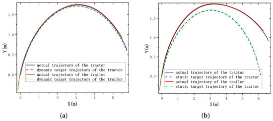
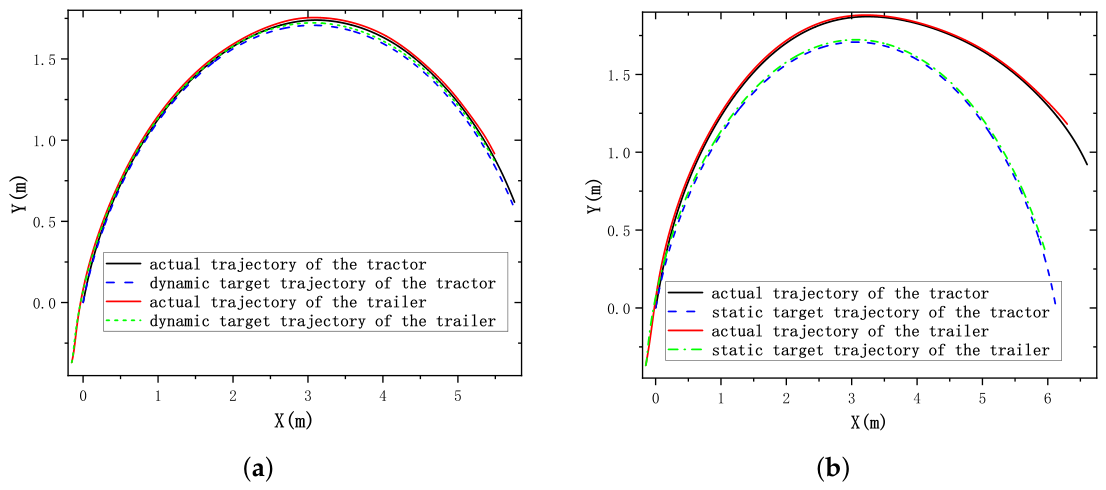
Figure 2 presents the trajectory tracking results of the off-axis trailer-type mobile structure under both static and dynamic reference targets. As shown in Figure 2a, the actual trajectory of the trailer closely tracks the desired reference trajectory with small tracking errors, and the lateral tracking error remains within a small range throughout the motion. Meanwhile, the actual trajectory of the trailer unit is also closely aligned with that of the tractor, exhibiting no evident deviation. These results indicate that, under the coordinated action of the dynamic tracking target and the passive steering angle, the curvature deviation induced by the off-axis trailer configuration can be effectively compensated. Consequently, the trailer is able to accurately follow the motion trajectory of the tractor, achieving accurate tracking of the reference trajectory and coordinated motion between the tractor and trailer.

In contrast, the tracking performance under the static reference target defined in (32) is noticeably degraded. The actual trajectory of the trailer exhibits an evident lateral deviation from the static reference path, gradually expanding outward as the traveled distance increases. This indicates that a fixed angular-velocity reference cannot adapt to the real-time motion state, leading to an inherent loss of trajectory accuracy even for the trailer itself. Under this condition, the deviation between the trailer and the tractor trajectories is further amplified. The trailer trajectory deviates significantly more than that of the tractor, and the consistency between the two is severely deteriorated. This phenomenon arises because the trajectory error of the trailer is transmitted to the trailer unit through the articulated joint structure; under the effect of the passive steering mechanism, this ultimately prevents the trailer from accurately following the tractor motion trajectory.

A comparison of the two cases demonstrates that the dynamic reference strategy significantly outperforms the static reference in both trajectory tracking accuracy and tractor–trailer coordination consistency. The dynamic reference, by updating the curvature in real time, ensures trajectory fidelity and provides a motion input consistent with the design requirements of the passive steering mechanism, thereby enabling coordinated high-precision tracking. In contrast, the static strategy suffers from intrinsic reference-path deviations, which are progressively amplified through the articulated structure, leading to a substantial degradation in the tracking performance of the trailer system.

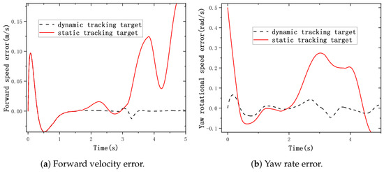
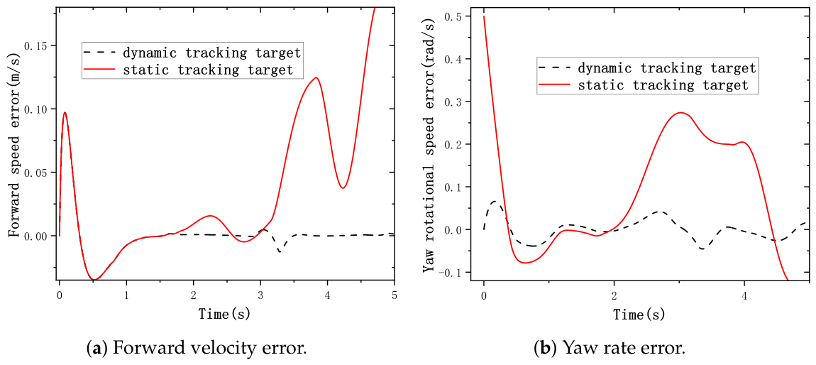
To further analyze the intrinsic reasons for the performance differences between the two trajectory tracking strategies, the tracking errors of the two key control variables, namely the forward velocity and the yaw rate of the tractor, are compared from the control perspective. The corresponding results are shown in Figure 3.

Under the dynamic reference case defined in (34), the forward velocity error exhibits a small transient fluctuation at the initial stage and then rapidly converges, remaining consistently around zero throughout the motion, which indicates excellent velocity tracking smoothness. The yaw rate error also decays quickly after the initial transient response and maintains a very small oscillation amplitude in steady state, demonstrating high tracking accuracy. In contrast, under the static reference case defined in (32), the forward velocity error converges rapidly at the beginning of the simulation; however, as the system enters the middle segment of the turning motion, the error magnitude gradually increases and exhibits persistent oscillations, failing to converge to a steady zero value. The yaw rate error shows a similar piecewise evolution: it decreases rapidly in the initial stage, then increases continuously in the curved segment, reaching its peak in the later part of the trajectory and exhibiting pronounced oscillations.

The superior tracking performance of the dynamic reference strategy can be attributed to the fact that the yaw rate reference is generated through the coupling between the intrinsic curvature of the reference path and the actual forward velocity, i.e., ${\omega }_d=v·{\kappa }_d,$ where ${\kappa }_d$ denotes the desired path curvature. This formulation allows the reference signal to be adaptively updated according to the system motion state. As long as the yaw rate accurately tracks the dynamic reference, the actual trajectory curvature remains consistent with the desired curvature, thereby eliminating the curvature deviation induced by velocity variations. In this case, the yaw rate tracking error is solely determined by the inherent capability of the controller and can therefore be maintained at a very low level.

Meanwhile, due to the coupling between the yaw rate reference and the forward velocity, no control conflict exists between the forward velocity channel and the yaw rate channel. The controller does not need to allocate control authority between speed tracking and trajectory correction. Consequently, the full control effort of the forward velocity channel can be devoted to disturbance rejection and velocity tracking, leading to fast convergence and high steady-state accuracy. Moreover, accurate forward velocity tracking further reinforces curvature matching, forming a benign closed-loop mechanism: $\mathrm{velocity}\mathrm{accuracy}\to \mathrm{curvature}\mathrm{matching}\to \mathrm{trajectory}\mathrm{stabilization}\to$ no additional velocity correction required.

For the static reference defined in (32), the yaw rate is a constant value. When the forward velocity deviates due to disturbances, dynamic coupling effects, or modeling uncertainties, even if the yaw rate can accurately track its reference value without error, the actual motion curvature will still deviate from the desired curvature, leading to an intrinsic and irreducible curvature mismatch. This deviation is continuously accumulated through the integral effect during trajectory tracking and is gradually transformed into position errors. In turn, the feedback correction of the position error forces the controller to increase the regulation effort on the yaw rate channel, thereby amplifying oscillations in the angular velocity response. Eventually, this leads to a positive error-feedback loop of the form: velocity deviation → curvature mismatch → position drift → yaw rate oscillation, which results in continuously increasing yaw rate errors accompanied by persistent oscillations. Once curvature mismatch induces trajectory deviation, the controller must allocate more control effort to the yaw rate channel in order to compensate for path errors. This inevitably reduces the available control bandwidth for the forward velocity channel, thereby degrading velocity tracking performance. As a result, a detrimental feedback loop is formed: velocity deviation → curvature deviation → path deviation → yaw rate compensation → further velocity deviation, which ultimately leads to increasing forward velocity errors and deteriorated steady-state performance.

From a kinematic perspective, the essence of trajectory tracking is to ensure consistency between the actual trajectory curvature and the desired trajectory curvature of the off-axis tractor-trailer wheeled mobile system. For wheeled mobile systems satisfying the pure rolling constraint, the trajectory curvature satisfies the relationship $\kappa =\omega /v$. Therefore, the performance difference between the two strategies can be clearly interpreted through the structure of curvature deviation.

For the dynamic reference strategy proposed in this paper, the reference yaw rate is constructed as ${\omega }_d=v·{\kappa }_d$, where ${\kappa }_d$ denotes the curvature of the desired trajectory. Substituting this relationship into the curvature expression yields

$$\kappa ={\displaystyle \frac{\omega }{v}}={\displaystyle \frac{{\omega }_d+e_{\omega }}{v}}={\kappa }_d+{\displaystyle \frac{e_{\omega }}{v}},$$

(37)

where the curvature deviation is given by $\mathsf{\Delta }\kappa =e_{\omega }/v$. It can be observed that the curvature error depends solely on the yaw rate tracking error and is independent of the forward velocity. This implies that velocity disturbances are not propagated into curvature deviations, thereby achieving decoupling between curvature tracking and velocity perturbations. This decoupling is the main reason for the superior tracking accuracy of the proposed dynamic strategy.

In contrast, for the conventional static reference strategy, the reference yaw rate ${\omega }_d$ is a constant. In this case, the actual curvature is given by

$$\kappa ={\displaystyle \frac{{\omega }_d+e_{\omega }}{v}},$$

(38)

and the corresponding curvature deviation can be decomposed into two terms:

$$\mathsf{\Delta }\kappa ={\displaystyle \frac{e_{\omega }}{v}}+{\displaystyle \frac{{\omega }_d-v{\kappa }_d}{v}},$$

(39)

where the first term represents the contribution of yaw rate tracking error, and the second term is the intrinsic curvature deviation induced by velocity mismatch with respect to the desired value. When velocity fluctuations occur, even if the yaw rate tracking error is negligible, the second term still leads to curvature mismatch. Moreover, the larger the velocity deviation, the more significant this intrinsic error becomes. This inherent limitation is the primary reason for the rapid deterioration of trajectory accuracy under the static reference strategy when subjected to velocity variations.

According to the above analysis, the proposed dynamic reference strategy consistently outperforms the static one in terms of trajectory tracking, forward velocity tracking, and yaw rate tracking. Among these, the improvement in forward velocity tracking is the most significant. By embedding the real-time forward velocity into the construction of the yaw rate reference, the dynamic strategy eliminates the control coupling between velocity and yaw rate, thereby achieving decoupling between curvature tracking and velocity disturbances. This effectively guarantees high-precision trajectory tracking performance. In contrast, the static strategy suffers from an intrinsic curvature deviation due to the mismatch between the constant yaw rate reference and the time-varying velocity. Moreover, competition for control bandwidth among different channels induces a positive error feedback mechanism, which leads to severe degradation of tracking performance in curved segments. As a result, the static strategy is only suitable for simple scenarios with nearly constant velocity and mild curvature variations.

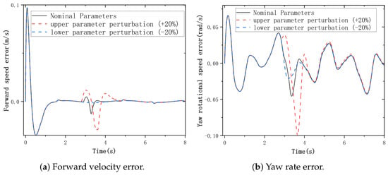
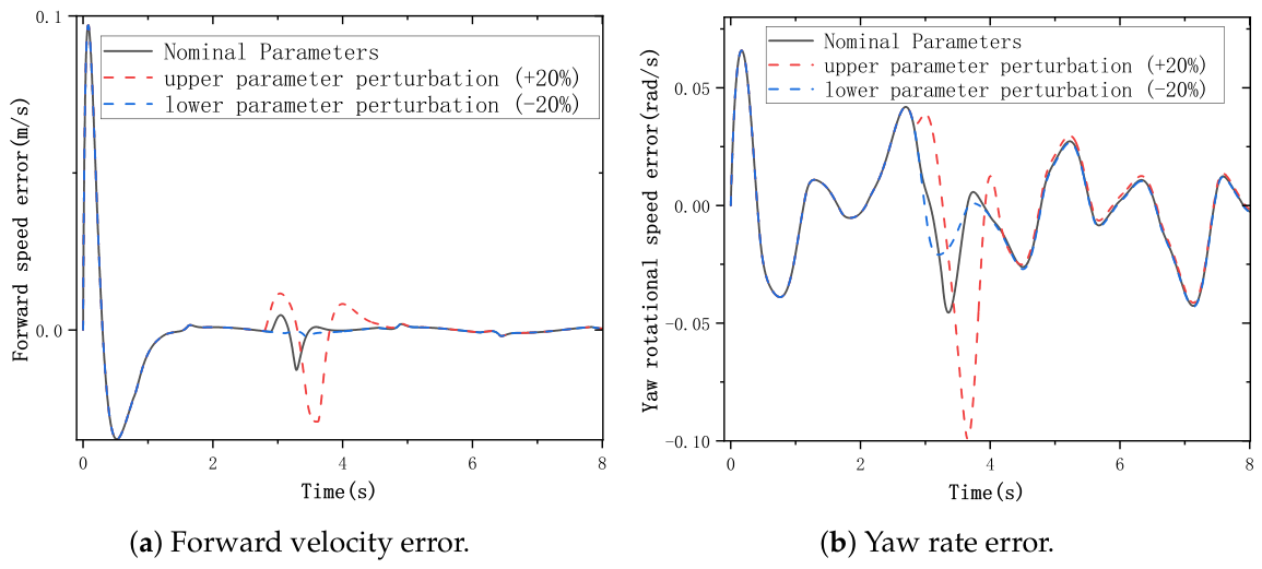
To further evaluate the robustness of the proposed control strategy, parameter uncertainties and measurement noise are considered in the following simulations. First, perturbations of $\pm 20\%$ are introduced into the key system parameters to investigate the influence of parameter uncertainties. The simulations are performed under the simultaneous effects of parameter variations and multi-frequency external disturbances.

The simulation results are summarized in

Table 1. Tracking performance (RMSE) under parameter uncertainties.

Parameter Variation	Longitudinal Velocity Error (m/s)	Yaw Rate Error (rad/s)	Lateral Deviation (m)
Nominal value	0.0147	0.0224	0.0368
+20%	0.0157 (+6.9%)	0.0284 (+26.5%)	0.0352 (−4.3%)
−20%	0.0146 (−0.5%)	0.0216 (−3.9%)	0.0397 (+7.8%)

. Under a positive parameter deviation of $+20\%$, the longitudinal velocity error and yaw-rate error increase by $6.9\%$ and $26.5\%$, respectively. For a negative parameter deviation of $-20\%$, the longitudinal velocity error and yaw-rate error change by $-0.5\%$ and $-3.9\%$, respectively, while the position error increases by $7.8\%$. In all parameter perturbation cases, the trajectory tracking error remains within $0.06$ m. These results indicate that the proposed controller maintains satisfactory tracking performance despite parameter variations. According to Equation (28), the sliding-mode dynamics of the disturbed system are expressed as

$$\dot{S}=-u_{xx}+\mathsf{\Delta }\left(t\right).$$

When the controller gains satisfy

$$k_{2i}>{\mathsf{\Delta }}_{i,\max }$$

and

$$k_{1i}>\sqrt{{\displaystyle \frac{2(k_{2i}+{\mathsf{\Delta }}_{i,\max })(1+p_i)}{(k_{2i}-{\mathsf{\Delta }}_{i,\max })(1-p_i)}}},$$

the sliding surface converges to zero within finite time. The parameter uncertainties are regarded as part of the total uncertainty and can be effectively compensated by the integral correction term. The tracking performance under parameter uncertainties is presented in Figure 4.

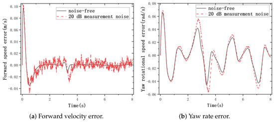
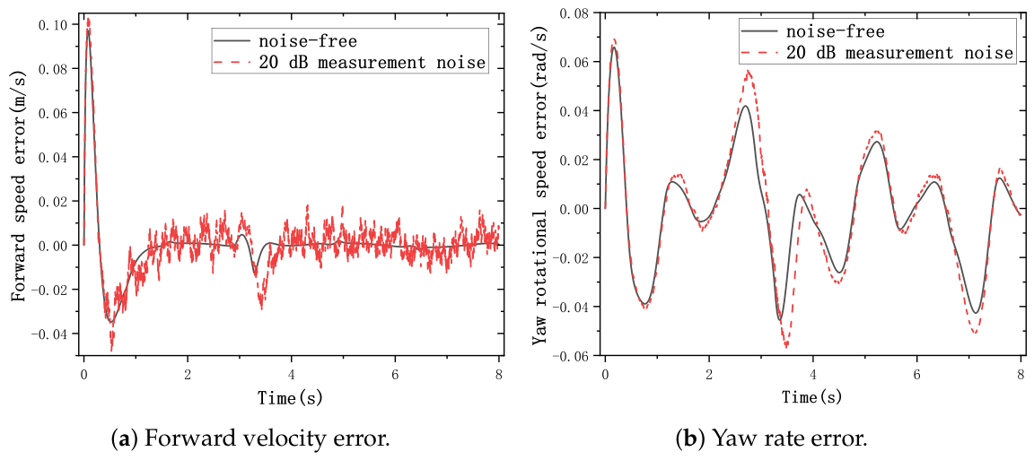
Furthermore, to simulate realistic sensor measurement conditions, Gaussian white noise with a signal-to-noise ratio of 20 dB is added to the longitudinal velocity and yaw-rate measurement channels. Owing to the smoothing approximation adopted in the super-twisting algorithm, $\mathrm{sgn}\left(S_i\right)\approx {\displaystyle \frac{S_i}{\epsilon +|S_i|}},$ where $\epsilon =0.005$, the amplification of measurement noise is effectively reduced.

As shown in

Table 2. Tracking performance (RMSE) under measurement noise.

Condition	Longitudinal Velocity Error (m/s)	Yaw-Rate Error (rad/s)	Lateral Deviation (m)
Without noise	0.0147	0.0224	0.0368
20 dB Gaussian white noise	0.0165 (+12.5%)	0.0269 (+19.6%)	0.0484 (+31.6%)

, under noisy measurement conditions, the longitudinal velocity error and yaw-rate error increase by $12.5\%$ and $19.6\%$, respectively. Nevertheless, the trajectory tracking accuracy remains better than the corresponding results obtained with the static tracking target. This demonstrates that the proposed controller possesses strong robustness against measurement noise. The tracking performance under measurement noise is illustrated in Figure 5.

Remark 2. 

Load variations can be essentially interpreted as changes in the mass parameters $M_f$ and $M_r$, which have already been considered in the parameter uncertainty analysis. Regarding wheel slip, this study is developed based on the pure rolling assumption, which provides a reasonable engineering approximation for low-speed motion conditions. For high-speed scenarios or low-adhesion surfaces, a wheel-slip model should be incorporated, which will be investigated in future work.

6.2. Comparison with Existing Control Methods

To further assess the effectiveness of the proposed controller, comparative simulations are carried out under the same cycloidal reference trajectory, disturbance conditions, and dynamic trajectory tracking framework. The proposed composite controller, referred to as ISMC-STA, is compared with two widely used trajectory tracking methods, namely the PID controller and the feedback linearization (FBL) controller. To ensure a fair comparison, all controllers adopt the same dynamic tracking target, and their parameters are carefully tuned to obtain satisfactory tracking performance.

For the PID controller, the known nonlinear dynamics of the system are utilized as feedforward compensation, while a PID feedback term is introduced to regulate the tracking errors. The control input is designed as

$${\mu }_{\mathrm{PID}}={\mathit{g}}^{-1}\left(\mathit{z}\right)\left({\dot{\mathit{z}}}_d-\mathit{f}\left(\mathit{z}\right)-{\mathit{K}}_P\mathit{e}-{\mathit{K}}_I{\int }_0^t\mathit{e}\left(\tau \right)\mathrm{d}\tau -{\mathit{K}}_D\dot{\mathit{e}}\right),$$

(40)

where ${\mathit{K}}_P$, ${\mathit{K}}_I$, and ${\mathit{K}}_D$ denote the proportional, integral, and derivative gain matrices, respectively. The feedforward component ${\dot{\mathit{z}}}_d-\mathit{f}\left(\mathit{z}\right)$ compensates for the nominal nonlinear dynamics, whereas the feedback component is responsible for reducing the remaining tracking errors. Although appropriate gain selection can ensure stable tracking, the PID controller does not explicitly compensate for external disturbances, which may deteriorate its tracking performance under persistent time-varying disturbances.

The FBL controller is constructed based on the same state-space model by cancelling the nonlinear terms and transforming the closed-loop system into a linear error dynamics. The corresponding control law is given by

$${\mu }_{\mathrm{FBL}}={\mathit{g}}^{-1}\left(\mathit{z}\right)\left({\dot{\mathit{z}}}_d-\mathit{f}\left(\mathit{z}\right)-\mathit{K}\mathit{e}\right),$$

(41)

where $\mathit{K}=\mathrm{diag}(k_1,k_2)$ is the feedback gain matrix. The resulting error dynamics can be expressed as $\dot{\mathit{e}}+\mathit{K}\mathit{e}=\mathbf{0},$ which ensures exponential convergence of the tracking error in the ideal model. However, the performance of FBL relies heavily on the accuracy of the system model. When parameter uncertainties $\mathsf{\Delta }\mathit{f}$, $\mathsf{\Delta }\mathit{g}$, or external disturbances are present, the nonlinear cancellation becomes incomplete, leading to an equivalent disturbance term $\mathsf{\Delta }\mathit{f}+\mathsf{\Delta }\mathit{g}{\mu }_{\mathrm{FBL}},$ which directly affects the tracking accuracy.

For the comparative study, the controller parameters are selected through repeated tuning. The parameters of the proposed ISMC-STA controller are set as $\lambda =\mathrm{diag}(5,0.3)$, $k_{11}=10$, $k_{12}=3.5$, $k_{21}=8$, $k_{22}=6$, and $\epsilon =0.02$. The PID gains are selected as ${\mathit{K}}_P=\mathrm{diag}(5,3)$, ${\mathit{K}}_I=\mathrm{diag}(2,1.5)$, and ${\mathit{K}}_D=\mathrm{diag}(0.1,0.05)$, while the FBL controller adopts $\mathit{K}=\mathrm{diag}(8,5)$. The same torque saturation constraint, $|{\mu }_i|\le 15\mathrm{N}·\mathrm{m},$ is imposed on all controllers.

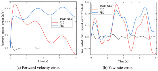
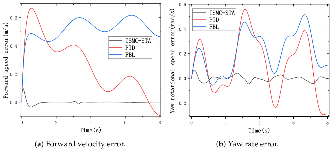
The quantitative comparison results are listed in

Table 3. Quantitative comparison of tracking performance among different controllers.

Performance Index	ISMC-STA	PID	FBL
Longitudinal velocity error RMSE (m/s)	0.0147	0.3273	0.5247
Yaw-rate error RMSE (rad/s)	0.0224	0.2544	0.2699
Maximum longitudinal velocity error (m/s)	0.0971	0.6669	0.6172
Maximum yaw-rate error (rad/s)	0.0659	0.5585	0.5155

. The proposed ISMC-STA controller achieves lower RMSE values in both longitudinal velocity and yaw-rate tracking errors compared with the PID and FBL controllers. Specifically, the RMSE values of the longitudinal velocity error and yaw-rate error are $0.0147$ m/s and $0.0224$ rad/s, respectively, while larger deviations are observed for the other two methods. Similar trends can also be found in terms of the maximum tracking errors, indicating that the proposed controller provides improved tracking performance under the considered disturbance conditions.

The corresponding tracking error responses are presented in Figure 6. Under disturbance-free conditions, all three controllers are capable of following the dynamic reference trajectory. However, when multi-frequency disturbances are introduced, the PID controller exhibits apparent steady-state oscillations due to the absence of an explicit disturbance compensation mechanism. The FBL controller shows increased tracking errors because its nonlinear cancellation capability is affected by model uncertainties and external disturbances. In contrast, the proposed ISMC-STA controller maintains stable tracking performance owing to the finite-time disturbance rejection property of the super-twisting algorithm. These comparisons verify the effectiveness of the proposed controller and demonstrate that the designed ISMC-STA scheme provides enhanced robustness for off-axis tractor-trailer wheeled mobile systems under disturbed operating conditions.

6.3. Tracking Results for S-Shaped and Circular Trajectories

To examine the adaptability of the proposed control strategy to different trajectory characteristics, additional simulations are conducted using two representative reference trajectories, namely an S-shaped trajectory with discontinuous curvature and a unit-circle trajectory with constant curvature. Except for the reference trajectories, all physical parameters, disturbance signals ${\mathsf{\Delta }}_1\left(t\right)$ and ${\mathsf{\Delta }}_2\left(t\right)$, and controller settings remain identical to those in the cycloidal trajectory case. Therefore, the influence of trajectory geometry on the tracking performance can be evaluated under the same operating conditions.

The S-shaped trajectory is constructed by connecting two circular arcs with opposite curvatures. The radius of each arc is selected as $R=1.5$ m, and the cruising velocity is set to $v_c=0.8$ m/s. A smooth acceleration-cruising-deceleration velocity profile is adopted throughout the motion. The curvature of the trajectory switches from $+1/R$ to $-1/R$ at the junction of the two arcs, resulting in a discontinuous curvature variation. This trajectory provides a representative test case for evaluating the tracking capability under abrupt changes in curvature. The S-shaped reference trajectory is expressed as

$$\widehat{\mathbf{r}}\left(s\right)=\left(x_d\left(s\right),y_d\left(s\right)\right),{\kappa }_d\left(s\right)=\left\{\begin{array}{cc}+1/R,\hfill & s\in [0,\pi R),\hfill \\ -1/R,\hfill & s\in [\pi R,2\pi R],\hfill \end{array}\right.$$

where s represents the arc-length parameter. The simulation duration is 10 s, and the initial condition is selected to coincide with the initial state of the reference trajectory.

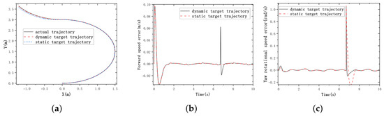
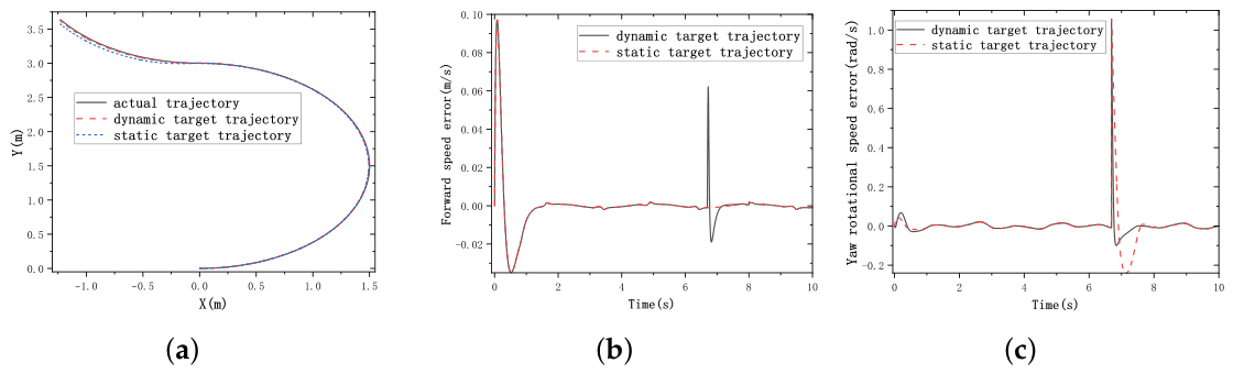
The tracking performances of the dynamic and static trajectory tracking targets are compared in

Table 4. Tracking performance comparison between the dynamic and static trajectory tracking targets for the S-shaped trajectory (RMSE).

Trajectory Target	Position Error (m)	Longitudinal Velocity Error (m/s)	Yaw-Rate Error (rad/s)	Maximum Position Error (m)
Dynamic trajectory	0.0091	0.0137	0.0514	0.0174
Static trajectory	0.0261	0.0131	0.0969	0.0488

. For the dynamic trajectory tracking target, the RMSE values of the position error, longitudinal velocity error, and yaw-rate error are $0.0091$ m, $0.0137$ m/s, and $0.0514$ rad/s, respectively. In contrast, the position error and yaw-rate error increase to $0.0261$ m and $0.0969$ rad/s under the static trajectory tracking target. The position tracking error is reduced by approximately $65\%$ with the dynamic trajectory tracking target. Although a transient fluctuation appears in the yaw-rate error when the curvature changes abruptly, the deviation is rapidly attenuated within approximately $0.5$ s due to the integral correction term introduced in the super-twisting algorithm. The corresponding tracking results are shown in Figure 7.

A unit-circle trajectory is further considered to evaluate the tracking performance under a constant-curvature condition. Such trajectories are commonly used as benchmark paths for continuous turning motions and can represent practical scenarios such as obstacle avoidance and cyclic transportation tasks. The curvature remains constant as $\kappa =1/R$ with $R=1.0$ m, and therefore $d\kappa /dt=0$. According to the theoretical analysis in Equation (37), the curvature deviation under the dynamic trajectory tracking target satisfies $\mathsf{\Delta }\kappa =e_{\omega }/v$. Since the curvature remains unchanged, the difference between the two tracking strategies is mainly reflected during the variable-speed phases, including acceleration and deceleration processes. The cruising velocity is selected as $v_c=0.8$ m/s, and the simulation duration is set to 10 s. The unit-circle trajectory is defined as

$$x_d\left(t\right)=R\cos \left({\omega }_{d}t\right),y_d\left(t\right)=R\sin \left({\omega }_{d}t\right),{\kappa }_d=1/R,$$

where ${\omega }_d=v/R$ denotes the desired yaw rate.

Table 5. Tracking performance comparison between the dynamic and static trajectory tracking targets for the unit-circle trajectory (RMSE).

Trajectory Target	Position Error (m)	Longitudinal Velocity Error (m/s)	Yaw-Rate Error (rad/s)	Maximum Position Error (m)
Dynamic trajectory	0.0111	0.0131	0.0223	0.0174
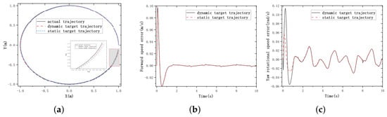
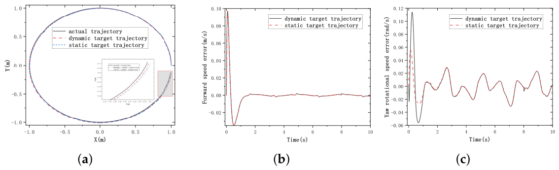
Static trajectory	0.0115	0.0131	0.0151	0.0174

summarizes the tracking performance comparison between the dynamic and static trajectory tracking targets. The RMSE values of the position error and yaw-rate error obtained with the dynamic trajectory tracking target are $0.0111$ m and $0.0223$ rad/s, respectively, while the corresponding values for the static trajectory tracking target are $0.0115$ m and $0.0151$ rad/s. The two strategies achieve comparable position tracking accuracy under constant curvature conditions. This is mainly because the curvature mismatch term $({\omega }_d-v{\kappa }_d)/v$ associated with the static trajectory tracking target remains relatively small when the curvature is constant. However, during the variable-speed phases, the dynamic trajectory tracking target maintains consistent tracking performance, whereas the static trajectory tracking target exhibits slight trajectory deviations. The tracking results for the unit-circle trajectory are presented in Figure 8.

The simulation results for the three representative trajectories demonstrate that the proposed control method achieves high-precision tracking performance under three distinct curvature conditions: continuously varying curvature (trochoidal trajectory), discontinuous curvature variation (S-shaped trajectory), and constant curvature (circular trajectory). These results verify the general applicability of the proposed method. The advantage of dynamic target trajectories is closely related to the curvature variation characteristics of the reference path. Specifically, the dynamic target trajectory exhibits significantly improved tracking performance over the static target trajectory in scenarios involving abrupt and varying curvature changes, whereas their performances become comparable for constant-curvature trajectories. This observation agrees well with the theoretical prediction given by Equations (37)–(39). The superiority of the dynamic target trajectory originates from the elimination of the inherent curvature mismatch term $({\omega }_d-v{\kappa }_d)/v$ caused by velocity inconsistency in the static target trajectory. When the curvature remains constant and the velocity is stable, this term becomes relatively small, leading to a reduced performance difference between the two approaches.

Remark 3. 

It should be emphasized that the core theoretical conclusion of this study, namely the curvature-error decoupling revealed by Equations (37)–(39), is derived without imposing any specific assumptions on the geometric form of the reference trajectory. In particular, the derivation of Equation (37) only relies on the curvature definition $\kappa =\omega /v$ and the dynamic target trajectory condition ${\omega }_d=v{\kappa }_d$, and therefore remains valid for any reference trajectory satisfying the following conditions: (i) the curvature ${\kappa }_d\left(s\right)$ exists and is continuous; (ii) the curvature is bounded, i.e., $|{\kappa }_d|\le {\kappa }_{\max }$; (iii) the reference trajectory is sufficiently smooth and differentiable. Under these conditions, dynamic trajectory tracking guarantees the curvature-error relation $\mathsf{\Delta }\kappa =e_{\omega }/v$, thereby achieving trajectory-independent curvature-error decoupling. This theoretical result is more general than conclusions obtained solely from numerical simulations. In this study, the trochoidal trajectory is selected as a validation case mainly because its curvature admits an analytical expression, $\kappa \left(s\right)=-{\displaystyle \frac{1}{\sqrt{16-16{\cos }^2(\pi /8)-s^2+8s\cos (\pi /8)}}},$ which provides an accurate benchmark for verifying the theoretical results in Equations (37)–(39). The selected trochoidal arc ($t\in [0,3\pi /2]$) exhibits a continuous curvature variation from $\kappa \left(0\right)$ to $\kappa (3\pi /2)$, covering typical road-curvature characteristics ranging from mild to sharp turns. Moreover, it includes curvature extrema, making it representative of general smooth paths with continuously varying curvature.

7. Conclusions

This paper investigates the accurate trajectory tracking problem of an off-axle trailer wheeled mobile structure. By exploiting the curvature consistency between the reference trajectory and the real-time motion state, a dynamic reference trajectory strategy is proposed. Combined with the passive steering mechanism, integral sliding surface, and super-twisting composite controller, a coordinated trajectory tracking framework for the tractor and trailer is developed. The simulation results lead to the following conclusions:

(i) Based on the intrinsic motion characteristics of the system, a passive steering angle is designed to enable the trailer to passively follow the trajectory of the tractor. Without introducing additional actuators or sensors for the trailer, the trajectory tracking task can be accomplished using only two driving torques of the tractor. This design significantly simplifies the control structure and reduces implementation complexity and cost.

(ii) The proposed dynamic reference trajectory strategy combines trajectory curvature with real-time motion states and ensures accurate tracking by regulating the curvature consistency. Compared with the conventional static reference trajectory, the proposed method effectively reduces the tracking errors of forward velocity and yaw rate, while suppressing trajectory deviation caused by error accumulation. Consequently, both tracking accuracy and robustness are significantly improved.

(iii) The passive steering mechanism and dynamic reference trajectory exhibit a strong synergistic effect. From both mechanical and control perspectives, high-precision coordinated trajectory tracking between the tractor and trailer is achieved. The trajectories of both units closely follow the desired path, demonstrating the effectiveness and feasibility of the proposed motion analysis, passive steering mechanism, and control strategy.

(iv) Comparative simulations with PID and feedback linearization controllers demonstrate the superiority of the proposed super-twisting composite controller, which achieves significant reductions in the root-mean-square errors of forward velocity and yaw rate. Furthermore, simulations under parameter uncertainties and measurement noises indicate that the proposed controller possesses strong robustness against system uncertainties and sensor disturbances. The results obtained from trochoidal, S-shaped, and circular trajectories further demonstrate the general applicability of the proposed strategy. In particular, the dynamic reference trajectory achieves substantial improvement under rapidly varying curvature conditions, while maintaining stable performance during constant-curvature and varying-speed motions.

It should be noted that the present results are obtained under the assumptions of low-speed motion and pure rolling conditions. Future work will consider more realistic engineering factors, including friction characteristics, actuator dynamics, and time-varying payloads, to establish a higher-fidelity dynamic model and provide more practical constraints for controller design. Moreover, semi-physical simulations and hardware experiments in ROS/Gazebo environments will be conducted to further evaluate the real-time performance and engineering applicability of the proposed method in complex scenarios. Owing to its simple structure and strong robustness, the proposed control strategy can provide theoretical guidance and technical support for accurate transportation of multi-trailer towing systems in confined environments, such as warehouse logistics, port transportation, and agricultural operations.

References

- David, J.; Manivannan, P.V. Control of truck-trailer mobile robots: A survey. Intell. Serv. Robot. 2014, 7, 245–258. [Google Scholar] [CrossRef] [Scilit]
- Zhao, H.; Liu, Z.; Li, Z.; Zhou, S.; Chen, W.; Suo, C.; Liu, Y.H. Modelling and dynamic tracking control of industrial vehicles with tractor-trailer structure. In Proceedings of the IEEE/RSJ International Conference on Intelligent Robots and Systems (IROS); IEEE: New York, NY, USA, 2019; pp. 2905–2910. [Google Scholar]
- Paszkowiak, W.; Bartkowiak, T.; Pelic, M. Kinematic model of a logistic train with a double Ackermann steering system. Int. J. Simul. Model. 2021, 20, 243–254. [Google Scholar] [CrossRef] [Scilit]
- Bin Salamah, Y. Sliding mode controller for autonomous tractor-trailer vehicle reverse path tracking. Appl. Sci. 2023, 13, 11998. [Google Scholar] [CrossRef] [Scilit]
- Yang, H.; Dang, R.; Li, P. Extended state observer-based trajectory tracking control of a wheeled mobile robot with one unpowered trailer. Asian J. Control 2025, 27, 1008–1019. [Google Scholar]
- Zhao, T.; Huang, W.; Xu, P.; Zhang, W.; Li, P.; Zhao, Y. A simple curvature-based backward path-tracking control for a mobile robot with N trailers. Actuators 2024, 13, 237. [Google Scholar] [CrossRef] [Scilit]
- Michalek, M.M.; Kielczewski, M.; Jedwabny, T. Cascaded VFO control for non-standard N-trailer robots. J. Intell. Robot. Syst. 2015, 77, 415–432. [Google Scholar]
- Rouchon, P.; Fliess, M.; Lévine, J.; Martin, P. Flatness, motion planning and trailer systems: An approach based on differential flatness. In Proceedings of the 32nd IEEE Conference on Decision and Control, San Antonio, TX, USA, 15–17 December 1993; pp. 2700–2705. [Google Scholar]
- Michalek, M.M. A highly scalable path-following controller for N-trailers with off-axle hitching. Control Eng. Pract. 2014, 29, 61–73. [Google Scholar] [CrossRef] [Scilit]
- Ljungqvist, O.; Evestedt, N.; Axehill, D.; Cirillo, M.; Pettersson, H. A path planning and path-following control framework for a general 2-trailer with a car-like tractor. J. Field Robot. 2019, 36, 1345–1370. [Google Scholar] [CrossRef] [Scilit]
- Khalaji, A.K.; Moosavian, S.A.A. Robust adaptive controller for a tractor-trailer mobile robot. IEEE/Asme Trans. Mechatron. 2014, 19, 943–953. [Google Scholar] [CrossRef] [Scilit]
- Khalaji, A.K.; Jalalnezhad, M. Control of a tractor-trailer robot subjected to wheel slip. Proc. Inst. Mech. Eng. Part K J. Multi-Body Dyn. 2019, 233, 875–891. [Google Scholar] [CrossRef] [Scilit]
- Leng, Z.; Minor, M.A. Curvature-based ground vehicle control of trailer path following considering sideslip and limited steering actuation. IEEE Trans. Intell. Transp. Syst. 2017, 18, 332–342. [Google Scholar] [CrossRef] [Scilit]
- Zhou, Y.; Chung, K. Path tracking control of a tractor-trailer wheeled robot kinematics with a passive steering angle. Appl. Math. Model. 2022, 109, 341–357. [Google Scholar] [CrossRef] [Scilit]
- Miao, S.; Zhou, Y. An identical path tracking control strategy of the tractor-trailer wheeled mobile robot with an off-axle hitching based on a passive steering angle. J. Frankl. Inst. 2024, 361, 106634. [Google Scholar] [CrossRef] [Scilit]
- Zhou, Y. Efficient path following control design for tractor with multiple trailers systems utilizing movement rules and passive multi-steering angles. Int. J. Robust Nonlinear Control 2025, 35, 3280–3296. [Google Scholar] [CrossRef] [Scilit]
- Shtessel, Y.; Edwards, C.; Fridman, L.; Levant, A. Sliding Mode Control and Observation; Birkhäuser: New York, NY, USA, 2014. [Google Scholar]
- Moreno, J.A.; Osorio, M. Strict Lyapunov functions for the super-twisting algorithm. IEEE Trans. Autom. Control 2012, 57, 1035–1040. [Google Scholar] [CrossRef] [Scilit]
Disclaimer/Publisher’s Note: The statements, opinions and data contained in all publications are solely those of the individual author(s) and contributor(s) and not of MDPI and/or the editor(s). MDPI and/or the editor(s) disclaim responsibility for any injury to people or property resulting from any ideas, methods, instructions or products referred to in the content. |
© 2026 by the authors. Licensee MDPI, Basel, Switzerland. This article is an open access article distributed under the terms and conditions of the Creative Commons Attribution (CC BY) license.