Review

Some Approaches to Solving the KP Equation: Different Representations and Various Types of Solutions

Unité Mixte de Recherche 5584, Institut de Mathématiques de Bourgogne, Centre National de la Recherche Scientifique, Université Bourgogne Europe, 21000 Dijon, France
Axioms 2026, 15(8), 586; https://doi.org/10.3390/axioms15080586
Submission received: 16 June 2026 / Revised: 13 July 2026 / Accepted: 21 July 2026 / Published: 4 August 2026
(This article belongs to the Special Issue Advances in Differential Equations and Its Applications)

Abstract

We present different methods to construct solutions to the Kadomtsev–Petviashvili (KP) equation. In the first method, from the solutions to the NLS equation, we construct solutions to the KP equation in terms of Fredholm determinants. We deduce solutions written as quotients of Wronskians of order 2 N . When one of these parameters tends to zero, we obtain N-order rational solutions expressed as a quotient of two polynomials of degree 2 N ( N + 1 ) in x, y and t, depending on 2 N 2 real parameters. We obtain, in this case, regular solutions to the KP equation. Using new results from the NLS equation, with solutions constructed in terms of quotients of determinants of order N depending on 2 N 2 real parameters, we are able to highlight new forms of configurations, such as triangles and concentric rings. Another approach using the Darboux transformation is given to get multi-parametric solutions to the KP equation. In this approach, it is possible to construct an infinite hierarchy of solutions depending on the degree of summation and the degree of derivation. The third method involves choosing special polynomials and using the bilinear Hirota method to get other types of solutions to the KP equation. We also obtain an infinite hierarchy of solutions depending on the order of the determinants. The last method allows the construction of regular solutions to the KP equation. In this approach, we obtain another alternative to obtain regular solutions, as in the case of the first method, and we also observe the formation of configurations such as triangles or concentric rings. We study the configurations of these hierarchies of solutions to the KP equation as a function of their different parameters.
MSC:
35C99; 35G20; 35Q35; 76B99; 76M99

1. Introduction

We consider the Kadomtsev–Petviashvili (KP) equation, which can be written as
( 4 u t 6 u u x + u x x x ) x = 3 u y y ,
where the subscripts x, y and t denote partial derivatives.
The KP equation is a universal integrable system in two spatial dimensions and has been extensively studied in the mathematical community.
The KP equation first appeared in 1970, in a paper written by Kadomtsev and Petviashvili [1]. This equation has been used as a model, for example, for surface and internal water waves by Ablowitz and Segur [2] and for nonlinear optics by Pelinovsky, Stepanyants and Kivshar [3].
The discovery of the KP equation happened almost simultaneously with the development of the inverse scattering transform (IST), as explained by Manakov et al. [4]. This method for constructing solutions to initial-value problems for nonlinear partial differential equations was originally developed for equations in one spatial dimension. However, in 1974 Dryuma showed how the KP equation could be written in Lax form [5]. Then, in the same year, Zakharov extended the IST method to equations in two spatial dimensions, including the KP equation, and obtained several exact solutions to the KP equation. The IST was applied by Prinari to obtain more general solutions to the KP equation [6] in 1999.
In parallel with the IST method, other equally important methods were developed almost simultaneously.
The algebro-geometric approach was used by Krichever to construct, for the first time in 1977 [7,8], solutions to the KP equation in terms of Riemann theta functions.
The Darboux method was also used by Matveev [9,10] in 1979 to obtain solutions to these equations.
Since 1980, a lot of methods have been applied to solve this equation, such as the non-local Riemann–Hilbert problem or the d-bar problem, as reviewed in the book by Ablowitz and Clarkson published in 1991 [11].
The Hirota bilinear method was used in [12] to construct solutions to the KP equation. Rational solutions of the KP hierarchy and the dynamics of their poles were given in [13] in 1998.
More recent relevant works should also be mentioned. A large variety of exact soliton solutions to the KP equation were given in the survey in [14], particularly localized solutions along certain lines in a two-dimensional plane, which decay exponentially everywhere else. A broad class of solutions to the KPI equation was constructed in 2021 by using a reduced version of the Grammian form of the τ function [15]. An algebro-geometric approach was proposed in [16], where solutions to the KP equation were constructed from certain degenerations of algebraic curves. Pattern formations in higher-order lumps of the KPI equation were studied at large time scales in [17]. The connection between the theory of integer partitions and a class of the KPI equation was studied in [18], and multi-lump patterns were given. Multi-lump formations from lump chains were studied in [19]. Also, multi-lump solutions to the KPI were constructed in [20] and characterized in terms of the partitions of a positive integer. The τ functions of regular KP solitons from totally non-negative Grassmannians were studied in [21], and it was proven that they can be expressed by Riemann theta functions on singular curves.
We present different methods to construct solutions to this equation.
From the solutions to the nonlinear Schrödinger (NLS) equation, we construct solutions to the KP equation in terms of Fredholm determinants. We deduce solutions written as quotients of Wronskians of order 2 N . These solutions, called solutions of order N, depend on 2 N 2 real parameters. When one of these parameters tends to zero, we obtain N-order rational solutions expressed as a quotient of two polynomials of degree 2 N ( N + 1 ) in x, y and t depending on 2 N 2 real parameters.
Another approach with the Darboux transformation is used to get multi-parametric solutions to the KP equation.
In the third approach, we choose special polynomials to get other types of solutions to the KP equation.
The last method allows the construction of regular solutions to the KP equation.
In the case of regular solutions, solution configurations in the form of triangles or concentric rings are related to the roots of the Vorobev–Yablonski and Ummemura polynomials, as mentioned in [22].

2. From the NLS Equation

2.1. Solution in Terms of Fredholm Determinants

In the following, we need to define some notations. First of all, one defines real numbers λ ν such that 1 < λ ν < 1 , ν = 1 , , 2 N , which depend on the parameter ϵ , which will tend towards 0; they can be written as
λ j = 1 2 ϵ 2 j 2 , λ N + j = λ j , 1 j N ,
The terms κ ν , δ ν , γ ν and x r , ν are functions of λ ν , 1 ν 2 N ; they are defined by the following formulas:
κ j = 2 1 λ j 2 , δ j = κ j λ j , γ j = 1 λ j 1 + λ j , ; x r , j = ( r 1 ) ln γ j i γ j + i , r = 1 , 3 , τ j = 12 i λ j 2 1 λ j 2 4 i ( 1 λ j 2 ) 1 λ j 2 , κ N + j = κ j , δ N + j = δ j , γ N + j = γ j 1 , x r , N + j = x r , j , , τ N + j = τ j j = 1 , , N .
e ν ,   1 ν 2 N , is defined in the following way:
e j = 2 i k = 1 1 / 2 M 1 a k ( j e ) 2 k 1 i k = 1 1 / 2 M 1 b K ( j e ) 2 k 1 , e N + j = 2 i k = 1 1 / 2 M 1 a k ( j e ) 2 k 1 + i k = 1 1 / 2 M 1 b k ( j e ) 2 k 1 , 1 j N , a k , b k R , 1 k N .
ϵ ν , 1 ν 2 N , denotes real numbers defined by
ϵ j = 1 , ϵ N + j = 0 1 j N .
Let I be the unit matrix and D r = ( d j k ) 1 j , k 2 N be a matrix defined by
d ν μ = ( 1 ) ϵ ν η μ γ η + γ ν γ η γ μ exp ( i κ ν x 2 δ ν y + τ ν t + x r , ν + e ν ) .
Then we have the following result.
Theorem 1. 
The function v defined by
v ( x , y , t ) = 2 n ( x , y , t ) 2 d ( x , y , t ) 2
where
n ( x , y , t ) = det ( I + D 3 ( x , y , t ) ) ,
d ( x , y , t ) = det ( I + D 1 ( x , y , t ) ) ,
with D r = ( d j k ) 1 j , k 2 N being a matrix defined by
d ν μ = ( 1 ) ϵ ν η μ γ η + γ ν γ η γ μ exp ( i κ ν x 2 δ ν y + τ ν t + x r , ν + e ν ) ,
is a solution to the KP Equation (1) depending on 2 N 2 parameters, a k and b h , 1 k N 1 .
Proof. 
From [23], the solution v to the one-dimensional focusing NLS equation can be written as
v ( x , t ) = det ( I + Δ 3 ( x , t ) ) det ( I + Δ 1 ( x , t ) ) exp ( 2 i t i φ ) ,
with Δ r = ( d j k ) 1 j , k 2 N being a matrix defined by
Δ ν μ = ( 1 ) ϵ ν η μ γ η + γ ν γ η γ μ exp ( i κ ν x 2 δ ν t + τ ν z + x r , ν + e ν ) .
where κ ν , δ ν , x r , ν , γ ν , τ ν , e ν , and ϵ ν are defined in (2)–(5), with the term z being another arbitrary real parameter.
The link between the solutions to the NLS equation and those to the KP equation was mentioned in preceding works; for example, it is explained in [24]. Specifically, the knowledge of a solution u that depends on x , t of the NLS equation can give a solution to the KP equation. For the solution u ( x , t ) to the NLS equation, we construct the function defined by u ˜ ( x , y , z ) for z, another variable. We make the substitutions t y and then z t , and then the function v defined by
v = 2 u ( x , y , t ) u * ( x , y , t ) ,
where * has the usual meaning of a complex conjugate, is a solution to the KP equation.
The problem is to determine the coefficient of the complementary real term z and make the preceding substitutions.
From the work of Bobenko and Bordag [25], it is clear that the coefficients in x, y and t of the solution to the KP equation must verify some explicit relations. Based on this crucial remark, it is clear that the coefficient of z can be nothing other than τ j = 12 i λ j 2 1 λ j 2 4 i ( 1 λ j 2 ) 1 λ j 2 .
From this expression, we can deduce the arguments of functions defined in matrices D 3 and D 1 ; they can be written as
( 1 ) ϵ ν η μ γ η + γ ν γ η γ μ exp ( i κ ν x 2 δ ν t + τ ν z + x r , ν + e ν ) .
Then, using the preceding result from the author of [23], recalled in (11), and making the substitutions t y and z t , it is clear that the solution to the KP equation takes the form
v ( x , y , t ) = 2 det ( I + D 3 ( x , y , t ) ) 2 det ( I + D 1 ( x , y , t ) ) ) 2
with the matrix D r defined in (10).
So we get the Fredholm representation (7) of the solutions to the KP equation. □

2.2. Solution in Terms of Wronskians

We want to express solutions to the NLS equation in terms of Wronskians. For this, we need the following notations:
ϕ r , ν = sin Θ r , ν , 1 ν N , ϕ r , ν = cos Θ r , ν , N + 1 ν 2 N , r = 1 , 3 ,
with the arguments
Θ r , ν = κ ν x 2 + i δ ν y i x r , ν 2 i τ ν 2 t + γ ν w i e ν 2 , 1 ν 2 N .
We denote by W r ( w ) the Wronskian of the functions ϕ r , 1 , , ϕ r , 2 N ; it is defined by
W r ( w ) = det [ ( w μ 1 ϕ r , ν ) ν , μ [ 1 , , 2 N ] ] .
We consider the matrix D r = ( d ν μ ) ν , μ [ 1 , , 2 N ] defined in (10). Then we have the following theorem.
Theorem 2. 
det ( I + D r ) = k r ( 0 ) × W r ( ϕ r , 1 , , ϕ r , 2 N ) ( 0 ) ,
where
k r ( w ) = 2 2 N exp ( i ν = 1 2 N Θ r , ν ) ν = 2 2 N μ = 1 ν 1 ( γ ν γ μ ) .
Proof. 
First, we remove the factor ( 2 i ) 1 e i Θ r , ν from each row ν in the Wronskian W r ( w ) for 1 ν 2 N .
Then
W r = ν = 1 2 N e i Θ r , ν ( 2 i ) N ( 2 ) N × W ˜ r ,
with
W ˜ r = ( 1 e 2 i Θ r , 1 ) i γ 1 ( 1 + e 2 i Θ r , 1 ) ( i γ 1 ) 2 N 1 ( 1 + ( 1 ) 2 N e 2 i Θ r , 1 ) ( 1 e 2 i Θ r , 2 ) i γ 2 ( 1 + e 2 i Θ r , 2 ) ( i γ 2 ) 2 N 1 ( 1 + ( 1 ) 2 N e 2 i Θ r , 2 ) ( 1 e 2 i θ r , 2 N ) i γ 2 N ( 1 + e 2 i Θ r , 2 N ) ( i γ 2 N ) 2 N 1 ( 1 + ( 1 ) 2 n e 2 i Θ r , 2 N )
The determinant W ˜ r can be written as
W ˜ r = det ( α j k e j + β j k ) ,
where α j k = ( 1 ) k ( i γ j ) k 1 , e j = e 2 i Θ r , j , and β j k = ( i γ j ) k 1 , 1 j N , 1 k 2 N , and α j k = ( 1 ) k 1 ( i γ j ) k 1 , e j = e 2 i Θ r , j , and β j k = ( i γ j ) k 1 , N + 1 j 2 N , 1 k 2 N . □
We want to calculate W ˜ r . To do this, we use the following lemma.
Lemma 1. 
Let A = ( a i j ) i , j [ 1 , . . . , N ] , B = ( b i j ) i , j [ 1 , . . . , N ] , and ( H i j ) i , j [ 1 , , N ] be a matrix formed by replacing the jth row in A with the ith row of B. Then
det ( a i j x i + b i j ) = det ( a i j ) × det ( δ i j x i + det ( H i j ) det ( a i j ) )
Proof. 
We use the classical notations: A ˜ = ( a ˜ j i ) i , j [ 1 , , N ] is the transposed matrix of cofactors of A. We have the well-known formula A × A ˜ = det A × I .
So it is clear that det ( A ˜ ) = ( det ( A ) ) N 1 .
The general term of the product ( c i j ) i , j [ 1 , . . , N ] = ( a i j x i + b i j ) i , j [ 1 , . . , N ] × ( a ˜ j i ) i , j [ 1 , . . , N ] can be written as
c i j = s = 1 N ( a i s x i + b i s ) × a ˜ j s = x i s = 1 n a i s a ˜ j s + s = 1 n b i s a ˜ j s = δ i j det ( A ) x i + det ( H i j ) .
We get
det ( c i j ) = det ( a i j x i + b i j ) × ( det ( A ) ) N 1 = ( det ( A ) ) N × det ( δ i j x i + det ( H i j ) det ( A ) ) .
Thus, det ( a i j x i + b i j ) = det ( A ) × det ( δ i j x i + det ( H i j ) det ( A ) ) .
We define U = ( α i j ) i , j [ 1 , , 2 N ] , V = ( β i j ) i , j [ 1 , , 2 N ] .
By applying the previous lemma, we obtain
W ˜ r = det ( α i j e i + β i j ) = det ( α i j ) × det ( δ i j e i + det ( H i j ) det ( α i j ) ) = det ( U ) × det ( δ i j e i + det ( H i j ) det ( U ) ) ,
where ( H i j ) i , j [ 1 , , N ] is the matrix formed by replacing the jth row in U with the ith row of V defined previously.
The determinant of U of the Vandermonde type is clearly equal to
det ( U ) = i N ( 2 N 1 ) 2 N l > m 1 ( γ l γ m ) .
To calculate the determinant W ˜ r , we must now compute det ( H i j ) . To do this, two cases must be studied.
1. For 1 j N . The matrix H i j is clearly of the Vandermonde type, where the j-th row in U is replaced by the i-th row of V. Clearly, we have
det ( H i j ) = ( 1 ) N ( 2 N + 1 ) + N 1 ( i ) N ( 2 N 1 ) × M ,
where M = M ( m 1 , , m 2 N ) is the Vandermonde determinant, defined by m k = γ k for k j and m j = γ i . Thus we have
det ( H i j ) = ( i ) N ( 2 N 1 ) × 2 N l > k 1 , ( m l m k ) = ( i ) N ( 2 N 1 ) × 2 N l > m 1 , l j , m j ( γ l γ m ) × l < j ( γ i γ l ) × l > j ( γ l + γ i ) , = ( 1 ) j ( i ) N ( 2 N 1 ) × 2 N l > m 1 , l j , m j ( γ l γ m ) × l j ( γ l + γ i ) .
To evaluate W ˜ r , we must simplify the quotient q i j : = det ( H i j ) det ( U ) :
q i j = ( 1 ) j ( i ) N ( 2 N 1 ) × 2 N l > m 1 , l j , m j ( γ l γ m ) × l j ( γ l + γ i ) i N ( 2 N 1 ) 2 N l > m 1 ( γ l γ m ) = ( 1 ) j l j ( γ l + γ i ) l < j ( γ j γ l ) l > j ( γ l γ j ) = ( 1 ) j l j ( γ l + γ i ) ( 1 ) j 1 l j ( γ l γ j ) = l j ( γ l + γ i ) l j ( γ l γ j ) .
We can replace q i j by r i j , defined by l j ( γ l + γ i ) l i ( γ l γ i ) , because det ( δ i j x i + det ( q i j ) det ( A ) ) = det ( δ i j x i + det ( r i j ) det ( A ) ) (similar matrices).
So the term r i j can be written as
r i j = ( 1 ) ϵ i l j γ l + γ i γ l γ j = c i j e 2 i Θ r , i ( 0 ) ,
with respect to the notations given (10).
2. The same estimations for N + 1 j 2 N are made; first, det H i j is
det ( H i j ) = ( 1 ) N ( 2 N + 1 ) + N 1 ( i ) N ( 2 N 1 ) × M ,
where M = M ( m 1 , , m 2 N ) is the Vandermonde determinant defined by m k = γ k for k j and m j = γ i . Thus we have
det ( H i j ) = ( i ) N ( 2 N 1 ) × 2 N l > k 1 , ( m l m k ) = ( i ) N ( 2 N 1 ) × 2 N l > m 1 , l j , m j ( γ l γ m ) × l < j ( γ i γ l ) × l > j ( γ l + γ i ) , = ( 1 ) j 1 ( i ) N ( 2 N 1 ) × 2 N l > m 1 , l j , m j ( γ l γ m ) × l j ( γ l + γ i ) .
The quotient q i j : = det ( H i j ) det ( U ) equals
q i j = ( 1 ) j 1 ( i ) N ( 2 N 1 ) × 2 N l > m 1 , l j , m j ( γ l γ m ) × l j ( γ l + γ i ) i N ( 2 N 1 ) 2 N l > m 1 ( γ l γ m ) = ( 1 ) j 1 l j ( γ l + γ i ) l < j ( γ j γ l ) l > j ( γ l γ j ) = ( 1 ) j 1 l j ( γ l + γ i ) ( 1 ) j 1 l j ( γ l γ j ) = l j ( γ l + γ i ) l j ( γ l γ j ) .
We replace q i j by r i j , defined by l j ( γ l + γ i ) l i ( γ l γ i ) , for the same reason as previously given.
So the term r i j can be written as
r i j = ( 1 ) ϵ i l j γ l + γ i γ l γ i = ( 1 ) ϵ ( i ) l j γ l + γ i l i γ l γ i = c i j e 2 i Θ r , i ( 0 ) ,
with respect to the notations given in (10).
By replacing e i with e 2 i Θ r , i , det W ˜ r can be expressed as
det W ˜ r = det ( U ) × det ( δ i j e i + det ( H i j ) det ( U ) ) = det ( U ) × det ( δ i j e i + r i j ) = det ( U ) i = 1 2 N e 2 i Θ i det ( δ i j + ( 1 ) ϵ ( i ) l i γ l + γ i γ l γ i e 2 i Θ r , i ) .
We estimate the two members of the last relation (29) for y = 0 , and using (20), we obtain the following result:
det W ˜ r ( 0 ) = i N ( 2 N 1 ) 2 N l > m 1 ( γ l γ m ) i = 1 2 N e 2 i Θ r , i ( 0 ) × det ( δ i j + ( 1 ) ϵ ( i ) l i γ l + γ i γ l γ i e 2 i Θ r , i ( 0 ) ) = i N ( 2 N 1 ) j = 2 2 N i = 1 j 1 ( γ j γ i ) e 2 i i = 1 2 N Θ r , i ( 0 ) det ( δ i j + c i j ) = i N ( 2 N 1 ) j = 2 2 N i = 1 j 1 ( γ j γ i ) e 2 i i = 1 2 N Θ r , i ( 0 ) det ( I + C r ) = i N ( 2 N 1 ) j = 2 2 N i = 1 j 1 ( γ j γ i ) e 2 i i = 1 2 N Θ r , i ( 0 ) det ( I + D r ) .
Therefore, the Wronskian W r given by (17) can be written as
W r ( ϕ r , 1 , , ϕ r , 2 N ) ( 0 ) = j = 1 2 N e i Θ r , j ( 0 ) ( 2 ) 2 N ( i ) N × W ˜ r = j = 1 2 N e i Θ r , j ( 0 ) ( 2 ) 2 N ( i ) N i N ( 2 N 1 ) j = 2 2 N i = 1 j 1 ( γ j γ i ) e 2 i i = 1 2 N Θ r , i ( 0 ) det ( I + D r ) = ( 2 ) 2 N j = 2 2 N i = 1 j 1 ( γ j γ i ) e i i = 1 2 N Θ r , i ( 0 ) det ( I + D r ) .
As a consequence,
det ( I + D r ) = k r ( 0 ) W r ( ϕ 1 , , ϕ 2 N ) ( 0 ) .
From the initial formulation, the solution v to the KP equation can be written as
v ( x , y , t ) = det ( I + D 3 ( x , y , t ) ) 2 det ( I + D 1 ( x , y , t ) ) 2 .
Using (16), the following relation between Fredholm determinants and Wronskians is obtained:
det ( I + D 3 ) = k 3 ( 0 ) × W 3 ( ϕ r , 1 , , ϕ r , 2 N ) ( 0 )
and
det ( I + D 1 ) = k 1 ( 0 ) × W 1 ( ϕ r , 1 , , ϕ r , 2 N ) ( 0 ) .
As Θ 3 , j ( 0 ) contains N terms x 3 , j 1 j N and N terms x 3 , j 1 j N , we have the equality k 3 ( 0 ) = k 1 ( 0 ) , and we get the following result.
Theorem 3. 
The function v defined by
v ( x , y , t ) = W 3 ( ϕ 3 , 1 , , ϕ 3 , 2 N ) ( 0 ) 2 W 1 ( ϕ 1 , 1 , , ϕ 1 , 2 N ) ( 0 ) 2
is a solution to the KP Equation (1) depending on 2 N 1 real parameters, a k , b k and ϵ, with ϕ ν r defined in (13),
ϕ r , ν = sin ( κ ν x 2 + i δ ν y i x r , ν 2 i τ ν 2 t + γ ν w i e ν 2 ) , 1 ν N , ϕ r , ν = cos ( κ ν x 2 + i δ ν y i x r , ν 2 i τ ν 2 t + γ ν w i e ν 2 ) , N + 1 ν 2 N , r = 1 , 3 ,
and with κ ν , δ ν , x r , ν , γ ν , e ν defined in (3), (2) and (4).

2.3. Rational Solutions

From the two preceding results, we construct rational solutions to the KP equation as a quotient of two determinants.
We use the following notations:
X ν = κ ν x 2 + i δ ν t i x 3 , ν 2 i τ ν t 2 i x 3 , ν 2 i e ν 2 ,
Y ν = κ ν x 2 + i δ ν t i x 3 , ν 2 i τ ν t 2 i e ν 2 ,
for 1 ν 2 N , with κ ν , δ ν , and x r , ν defined in (3) and parameter e ν defined in (4).
We define the following functions:
φ 4 j + 1 , k = γ k 4 j 1 sin X k , φ 4 j + 2 , k = γ k 4 j cos X k , φ 4 j + 3 , k = γ k 4 j + 1 sin X k , φ 4 j + 4 , k = γ k 4 j + 2 cos X k ,
for 1 k N , and
φ 4 j + 1 , N + k = γ k 2 N 4 j 2 cos X N + k , φ 4 j + 2 , N + k = γ k 2 N 4 j 3 sin X N + k , φ 4 j + 3 , N + k = γ k 2 N 4 j 4 cos X N + k , φ 4 j + 4 , N + k = γ k 2 N 4 j 5 sin X N + k ,
for 1 k N .
We define the function ψ j , k for 1 j 2 N , 1 k 2 N , in the same way, except the term X k is replaced by Y k .
ψ 4 j + 1 , k = γ k 4 j 1 sin Y k , ψ 4 j + 2 , k = γ k 4 j cos Y k , ψ 4 j + 3 , k = γ k 4 j + 1 sin Y k , ψ 4 j + 4 , k = γ k 4 j + 2 cos Y k ,
for 1 k N , and
ψ 4 j + 1 , N + k = γ k 2 N 4 j 2 cos Y N + k , ψ 4 j + 2 , N + k = γ k 2 N 4 j 3 sin Y N + k , ψ 4 j + 3 , N + k = γ k 2 N 4 j 4 cos Y N + k , ψ 4 j + 4 , N + k = γ k 2 N 4 j 5 sin Y N + k ,
for 1 k N .
The ratio
q ( x , t ) : = W 3 ( 0 ) W 1 ( 0 )
can be written as
q ( x , t ) = Δ 3 Δ 1 = det ( φ j , k ) j , k [ 1 , 2 N ] det ( ψ j , k ) j , k [ 1 , 2 N ] .
The terms λ j depending on ϵ are defined by λ j = 1 2 j ϵ 2 . All functions φ j , k and ψ j , k and their derivatives depend on ϵ . They can all be prolonged by continuity when ϵ = 0 .
We use the following expansions:
φ j , k ( x , y , t , ϵ ) = l = 0 N 1 1 ( 2 l ) ! φ j , 1 [ l ] k 2 l ϵ 2 l + O ( ϵ 2 N ) , φ j , 1 [ l ] = 2 l φ j , 1 ϵ 2 l ( x , y , t , 0 ) ,
φ j , 1 [ 0 ] = φ j , 1 ( x , y , t , 0 ) , 1 j 2 N , 1 k N , 1 l N 1 ,
φ j , N + k ( x , y , t , ϵ ) = l = 0 N 1 1 ( 2 l ) ! φ j , N + 1 [ l ] k 2 l ϵ 2 l + O ( ϵ 2 N ) , φ j , N + 1 [ l ] = 2 l φ j , N + 1 ϵ 2 l ( x , y , t , 0 ) ,
φ j , N + 1 [ 0 ] = φ j , N + 1 ( x , y , t , 0 ) , 1 j 2 N , 1 k N , 1 l N 1 .
We have the same expansions for the functions ψ j , k .
ψ j , k ( x , y , t , ϵ ) = l = 0 N 1 1 ( 2 l ) ! ψ j , 1 [ l ] k 2 l ϵ 2 l + O ( ϵ 2 N ) , ψ j , 1 [ l ] = 2 l ψ j , 1 ϵ 2 l ( x , y , t , 0 ) ,
ψ j , 1 [ 0 ] = ψ j , 1 ( x , y , t , 0 ) , 1 j 2 N , 1 k N , 1 l N 1 ,
ψ j , N + k ( x , t , ϵ ) = l = 0 N 1 1 ( 2 l ) ! ψ j , N + 1 [ l ] k 2 l ϵ 2 l + O ( ϵ 2 N ) , ψ j , N + 1 [ l ] = 2 l ψ j , N + 1 ϵ 2 l ( x , y , t , 0 ) ,
ψ j , N + 1 [ 0 ] = ψ j , N + 1 ( x , t , 0 ) , 1 j 2 N , 1 k N , N + 1 k 2 N . .
Then we get the following result.
Theorem 4. 
The function v defined by
v ( x , y , t ) = 2 | det ( ( n j k ) j , k [ 1 , 2 N ] ) | 2 det ( ( d j k ) j , k [ 1 , 2 N ] ) 2
is a rational solution to the KP Equation (1).
( 4 u t 6 u u x + u x x x ) x 3 u y y = 0 ,
where
n j 1 = φ j , 1 ( x , y , t , 0 ) , 1 j 2 N n j k = 2 k 2 φ j , 1 ϵ 2 k 2 ( x , y , t , 0 ) , n j N + 1 = φ j , N + 1 ( x , y , t , 0 ) , 1 j 2 N n j N + k = 2 k 2 φ j , N + 1 ϵ 2 k 2 ( x , y , t , 0 ) , d j 1 = ψ j , 1 ( x , y , t , 0 ) , 1 j 2 N d j k = 2 k 2 ψ j , 1 ϵ 2 k 2 ( x , y , t , 0 ) , d j N + 1 = ψ j , N + 1 ( x , y , t , 0 ) , 1 j 2 N d j N + k = 2 k 2 ψ j , N + 1 ϵ 2 k 2 ( x , y , t , 0 ) , 2 k N , 1 j 2 N
The functions φ and ψ are defined in (33)–(36).
Proof. 
In each column k (and N + k ) of the determinants appearing in q ( x , t ) , we successively eliminate powers of ϵ strictly inferior to 2 ( k 1 ) ; then each common term in the numerator and denominator is factorized and simplified; and finally, we take the limit as ϵ goes to 0.
First, the components j of columns 1 and N + 1 are respectively equal, by definition, to φ j 1 [ 0 ] + 0 ( ϵ ) for C 1 , φ j N + 1 [ 0 ] + 0 ( ϵ ) for C N + 1 of Δ 3 , and ψ j 1 [ 0 ] + 0 ( ϵ ) for C 1 , ψ j N + 1 [ 0 ] + 0 ( ϵ ) for C N + 1 of Δ 1 .
In the first step of the reduction, we replace the columns C k by C k C 1 and C N + k by C N + k C N + 1 for 2 k N for Δ 3 ; the same changes are made for Δ 1 . Each component j of the column C k of Δ 3 can be rewritten as l = 1 N 1 1 ( 2 l ) ! φ j , 1 [ l ] ( k 2 l 1 ) ϵ 2 l , and the column C N + k can be replaced by l = 1 N 1 1 ( 2 l ) ! φ j , N + 1 [ l ] ( k 2 l 1 ) ϵ 2 l for 2 k N . For Δ 1 , we make the same reductions; each component j of the column C k can be rewritten as l = 1 N 1 1 ( 2 l ) ! ψ j , 1 [ l ] ( k 2 l 1 ) ϵ 2 l , and the column C N + k can be replaced by l = 1 N 1 1 ( 2 l ) ! ψ j , N + 1 [ l ] ( k 2 l 1 ) ϵ 2 l for 2 k N .
The term k 2 1 2 ϵ 2 for 2 k N can be factorized in Δ 3 and Δ 1 in each column k and N + k , so these common terms can be simplified in the numerator and denominator.
If we restrict the developments to order 1 in columns 2 and N + 2 , we respectively get φ j 1 [ 1 ] + 0 ( ϵ ) for component j of C 2 , φ j N + 1 [ 1 ] + 0 ( ϵ ) for component j of C N + 2 of Δ 3 , and ψ j 1 [ 1 ] + 0 ( ϵ ) for component j of C 2 , ψ j N + 1 [ 1 ] + 0 ( ϵ ) for component j of C N + 2 of Δ 1 . We can continue this algorithm up to columns C N , C 2 N of Δ 3 and C N , C 2 N of Δ 1 .
Then we take the limit as ϵ tends to 0, and q ( x , y , t ) can be replaced by Q ( x , y , t ) , defined by
Q ( x , y , t ) : = φ 1 , 1 [ 0 ] φ 1 , 1 [ N 1 ] φ 1 , N + 1 [ 0 ] φ 1 , N + 1 [ N 1 ] φ 2 , 1 [ 0 ] φ 2 , 1 [ N 1 ] φ 2 , N + 1 [ 0 ] φ 2 , N + 1 [ N 1 ] φ 2 N , 1 [ 0 ] φ 2 N , 1 [ N 1 ] φ 2 N , N + 1 [ 0 ] φ 2 N , N + 1 [ N 1 ] 2 ψ 1 , 1 [ 0 ] ψ 1 , 1 [ N 1 ] ψ 1 , N + 1 [ 0 ] ψ 1 , N + 1 [ N 1 ] ψ 2 , 1 [ 0 ] ψ 2 , 1 [ N 1 ] ψ 2 , N + 1 [ 0 ] ψ 2 , N + 1 [ N 1 ] ψ 2 N , 1 [ 0 ] ψ 2 N , 1 [ N 1 ] ψ 2 N , N + 1 [ 0 ] ψ 2 N , N + 1 [ N 1 ] 2
So the solution to the KP equation takes the form
v ( x , y , t ) = 2 Q ( x , y , t )
and we get the result. □

2.4. Another Representation of the Solutions to the KP Equation

By using the previous results, we can give another representation of the solutions to the KP equation depending only on the terms γ ν , 1 ν 2 N . This is done by expressing κ ν , δ ν , τ ν and x r , ν as functions of γ ν for 1 ν 2 N , and we get
κ j = 4 γ j ( 1 + γ j 2 ) , δ j = 4 γ j ( 1 γ j 2 ) ( 1 + γ j 2 ) 2 , x r , j = ( r 1 ) ln γ j i γ j + i , τ j = 8 i γ j ( 3 2 γ j 2 + 3 γ j 4 ) ( 1 + γ j 2 ) 3 , 1 j N , κ j = 4 γ j ( 1 + γ j 2 ) , δ j = 4 γ j ( 1 γ j 2 ) ( 1 + γ j 2 ) 2 , x r , j = ( r 1 ) ln γ j + i γ j i , τ j = 8 i γ j ( 3 2 γ j 2 + 3 γ j 4 ) ( 1 + γ j 2 ) 3 , N + 1 j 2 N .
We get the following representation.
Theorem 5. 
The function v defined by
v ( x , y , t ) = 2 det [ ( w μ 1 ϕ ˜ 3 , ν ( 0 ) ) ν , μ [ 1 , , 2 N ] ] 2 ( det [ ( w μ 1 ϕ ˜ 1 , ν ( 0 ) ) ν , μ [ 1 , , 2 N ] ] ) 2
is a solution to the KP Equation (1), with the functions ϕ ˜ r , ν being defined by
ϕ ˜ r , j ( w ) = sin 2 γ j ( 1 + γ j 2 ) x + i 4 γ j ( 1 γ j 2 ) ( 1 + γ j 2 ) 2 t 4 γ j ( 3 2 γ j 2 + 3 γ j 4 ) ( 1 + γ j 2 ) 3 y i ( r 1 ) 2 ln γ j i γ j + i + γ j w i e j 2 , ϕ ˜ r , N + j ( w ) = cos 2 γ j ( 1 + γ j 2 ) x i 4 γ j ( 1 γ j 2 ) ( 1 + γ j 2 ) 2 t 4 γ j ( 3 2 γ j 2 + 3 γ j 4 ) ( 1 + γ j 2 ) 3 + i ( r 1 ) 2 ln γ j i γ j + i + 1 γ j w i e N + j 2 , 1 j , N , w i t h e j = i k = 1 N 1 a k ϵ 2 k + 1 j 2 k + 1 k = 1 N 1 b k ϵ 2 k + 1 j 2 k + 1 , e N + j = i k = 1 N 1 a k ϵ 2 k + 1 j 2 k + 1 + k = 1 N 1 b k ϵ 2 k + 1 j 2 k + 1 , a i , b i   r e a l s 1 j N 1 .
Remark 1. 
In relation (41), the determinants det [ ( w μ 1 f ν ( 0 ) ) ν , μ [ 1 , , 2 N ] ] are Wronskians of the functions f 1 , , f 2 N evaluated at w = 0 . In particular, w 0 f ν means f ν .

2.5. Structure of the Rational Solutions

Here, we give a theorem that states, in this representation, the structure of the rational solutions to the KP equation. In this section we use the notations defined in the previous sections. The functions φ and ψ are defined in (33)–(36).
Theorem 6. 
The function v defined by
v ( x , y , t ) = 2 det ( ( n j k ) j , k [ 1 , 2 N ] ) 2 ( det ( ( d j k ) j , k [ 1 , 2 N ] ) ) 2
is a rational solution to the KP Equation (1) written as a quotient of two polynomials, n ( x , y , t ) and d ( x , y , t ) , depending on 2 N 2 real parameters a j and b j , 1 j N 1 .
n and d are polynomials of degree 2 N ( N + 1 ) in x, y and t.
The terms n j k and d j k are defined in (39), and the functions φ and ψ are defined in (33)–(36).
Proof. 
From the previous result (40), we have to analyze the functions φ k , 1 , ψ k , 1 and φ k , N + 1 , ψ k , N + 1 . The functions φ k , j and ψ k , j differ only in the term of the argument x 3 , k , so only the study of functions φ k , j will be carried out. Then we study functions ψ k , j , and the result can be easily deduced from the analysis of φ k , j .
We study the expansions of these functions in ϵ . We denote by ( l k j ) k , j [ 1 , 2 N ] the matrix defined by
l k j = 2 j 2 ϵ 2 j 2 φ k 1 , l k , j + N = 2 j 2 ϵ 2 j 2 φ k , 1 + N , 1 j N , 1 k 2 N ,
with 0 x 0 φ meaning φ . Each coefficient of the matrix ( l k j ) k , j [ 1 , 2 N ] must be evaluated for the power of x, y and t in the coefficient of ϵ 2 ( m 1 ) for the column m [ 1 , 2 N ] . We remark that with these notations, the matrix ( l k j ) k , j [ 1 , 2 N ] evaluated at ϵ = 0 is exactly ( n k j ) k , j [ 1 , 2 N ] , defined in (39). There are four cases to study, depending on the parity of k.
1. Case l k 1 for k odd, k = 2 s + 1 .
l k 1 = ( 1 ) s sin ( 2 ϵ ( 1 ϵ 2 ) 1 2 x + 4 i ϵ ( 1 ϵ 2 ) 1 2 ( 1 2 ϵ 2 ) y ( 12 ϵ ( 1 ϵ 2 ) 1 2 ( 1 2 ϵ 2 ) 2 + 16 ϵ 3 ( 1 ϵ 2 ) 3 2 ) t
i ln 1 + i ϵ ( 1 ϵ 2 ) 1 2 1 i ϵ ( 1 ϵ 2 ) 1 2 e 1 ) × ϵ k 2 ( 1 ϵ 2 ) k 2 2
= ( 1 ) s sin ϵ ( l = 0 p c 2 l ϵ 2 l x + 2 i l = 0 p c 2 l ϵ 2 l ( 1 2 ϵ 2 ) y + l = 0 p h 2 l ϵ 2 l t + 2 l = 0 p ( 1 ) l ϵ 2 l ( 1 ϵ 2 ) 2 l + 1 2 ( 2 l + 1 )
l = 1 N 1 a ˜ l ϵ 2 l + i l = 1 N 1 b ˜ l ϵ 2 l + O ( ϵ p + 1 ) ) × ϵ k 2 ( l = 1 r g 2 l ϵ 2 l + O ( ϵ r + 1 ) )
= ( 1 ) s sin ϵ ( l = 0 p ( c 2 l x + d 2 l y + h 2 l t + f 2 l + O ( ϵ p + 1 ) ) ϵ 2 l ) × ϵ k 2 ( l = 1 r g 2 l ϵ 2 l + O ( ϵ r + 1 ) )
= l = 0 q ( 1 ) l + s ϵ 2 l ( 2 l + 1 ) ! ( n = 0 p ( c 2 n x + d 2 n y + h 2 l t + f 2 n + O ( ϵ p + 1 ) ) ϵ 2 n ) 2 l + 1 × ϵ k 1 ( l = 1 r g 2 l ϵ 2 l + O ( ϵ r + 1 ) )
= l = 0 q ( 1 ) l + s ϵ 2 l ( 2 l + 1 ) ! ( n = 0 p P n ( x , y , t ) ϵ 2 n ) 2 l + 1 × ϵ k 1 l = 1 r g 2 l ϵ 2 l + O ( ϵ t )
where P n ( x , y , t ) is a polynomial of order 1 in x, y and t.
l k , 1 = l = 0 q ϵ 2 l α 0 + + α p = 2 l + 1 β α 0 , , α p P 0 ( x , y , t ) α 0 P p ( x , y , t ) α p ϵ 2 ( α 1 + 2 α 2 + p α p ) × ϵ 2 s l = 1 r g 2 l ϵ 2 l + O ( ϵ t )
= l = 0 q ϵ 2 l α 0 + + α p = 2 l + 1 Q α 0 , , α p ( x , y , t ) ϵ 2 ( α 1 + 2 α 2 + p α p ) × ϵ 2 s l = 1 r g 2 l ϵ 2 l + O ( ϵ t ) ,
where Q α 0 , , α p ( x , y , t ) is a polynomial of order 2 l + 1 in x, y and t.
The terms in ϵ 0 are obtained for l = 0 in the two summations with α 0 = 1 .
For the column m, we search the terms in ϵ 2 m 2 to find the one with the maximum power in x, y and t. It is obtained for 2 l + k 1 = 2 m 2 , which gives l = m s 1 .
We get the following result. □
Proposition 1. 
deg ( n 2 s + 1 , m ) = 2 ( m s ) 1   f o r   s m 1 , n 2 s + 1 , m = 0   f o r   s m .
2. Case l k 1 for k even, k = 2 s .
l k 1 = ( 1 ) s + 1 cos ( 2 ϵ ( 1 ϵ 2 ) 1 2 x + 4 i ϵ ( 1 ϵ 2 ) 1 2 ( 1 2 ϵ 2 ) y ( 12 ϵ ( 1 ϵ 2 ) 1 2 ( 1 2 ϵ 2 ) 2 + 16 ϵ 3 ( 1 ϵ 2 ) 3 2 ) t
i ln 1 + i ϵ ( 1 ϵ 2 ) 1 2 1 i ϵ ( 1 ϵ 2 ) 1 2 e 1 ) × ϵ k 2 ( 1 ϵ 2 ) k 2 2
= ( 1 ) s + 1 cos ϵ ( l = 0 p c 2 l ϵ 2 l x + 2 i l = 0 p c 2 l ϵ 2 l ( 1 2 ϵ 2 ) y + l = 0 p h 2 l ϵ 2 l t + 2 l = 0 p ( 1 ) l ϵ 2 l ( 1 ϵ 2 ) 2 l + 1 2 ( 2 l + 1 )
l = 1 N 1 a ˜ l ϵ 2 l + i l = 1 N 1 b ˜ l ϵ 2 l + O ( ϵ p + 1 ) ) × ϵ k 2 ( l = 1 r g 2 l ϵ 2 l + O ( ϵ r + 1 ) )
= ( 1 ) s + 1 cos ϵ ( l = 0 p ( c 2 l x + d 2 l y + h 2 y t + f 2 l + O ( ϵ p + 1 ) ) ϵ 2 l ) × ϵ k 2 ( l = 1 r g 2 l ϵ 2 l + O ( ϵ r + 1 ) )
= l = 0 q ( 1 ) l + d + 1 ϵ 2 l ( 2 l ) ! ( n = 0 p ( c 2 n x + d 2 n y + h 2 l t + f 2 n + O ( ϵ p + 1 ) ) ϵ 2 n ) 2 l × ϵ k 2 ( l = 1 r g 2 l ϵ 2 l + O ( ϵ r + 1 ) )
= l = 0 q ( 1 ) l + s + 1 ϵ 2 l ( 2 l ) ! ( n = 0 p P n ( x , y , t ) ϵ 2 n ) 2 l × ϵ 2 s 2 l = 1 r g 2 l ϵ 2 l + O ( ϵ t )
where P n ( x , y , t ) is a polynomial of order 1 in x, y and t.
l k , 1 = l = 0 q ϵ 2 l α 0 + + α p = 2 l β α 0 , , α p P 0 ( x , y , t ) α 0 P p ( x , y , t ) α p ϵ 2 ( α 1 + 2 α 2 + p α p ) × ϵ 2 s 2 l = 1 r g 2 l ϵ 2 l + O ( ϵ t )
= l = 0 q ϵ 2 l α 0 + + α p = 2 l Q α 0 , , α p ( x , y , t ) ϵ 2 ( α 1 + 2 α 2 + p α p ) × ϵ 2 s 2 l = 1 r g 2 l ϵ 2 l + O ( ϵ t ) ,
where Q α 0 , , α p ( x , y , t ) is a polynomial of order 2 l in x, y and t.
Terms in ϵ 0 are obtained for l = 0 in the two summations with α 0 = 1 .
For the column m, we search the terms in ϵ 2 m 2 to find the one with the maximum power in x and t. It is obtained for 2 l + k 2 = 2 m 2 , which gives l = m s .
So we have the following proposition.
Proposition 2. 
deg ( n 2 s , m ) = 2 ( m s )   f o r   s m , n 2 s , m = 0   f o r   s > m .
3. Case l k M 2 + 1 for k odd, k = 2 s + 1 .
l k M 2 + 1 = ( 1 ) s cos ( 2 ϵ ( 1 ϵ 2 ) 1 2 x 4 i ϵ ( 1 ϵ 2 ) 1 2 ( 1 2 ϵ 2 ) y + i ln 1 + i ϵ ( 1 ϵ 2 ) 1 2 1 i ϵ ( 1 ϵ 2 ) 1 2 e M 2 + 1
( 12 ϵ ( 1 ϵ 2 ) 1 2 ( 1 2 ϵ 2 ) 2 + 16 ϵ 3 ( 1 ϵ 2 ) 3 2 ) t )   ×   ϵ M k 1 ( 1 ϵ 2 ) M k 1 2
= ( 1 ) s ( cos ϵ ( l = 0 p c 2 l ϵ 2 l x 2 i l = 0 p c 2 l ϵ 2 l ( 1 2 ϵ 2 ) y + l = 0 p h 2 l ϵ 2 l t 2 l = 0 p ( 1 ) l ϵ 2 l ( 1 ϵ 2 ) 2 l + 1 2 ( 2 l + 1 )
l = 1 N 1 a ˜ l ϵ 2 l + i l = 1 N 1 b ˜ l ϵ 2 l + O ( ϵ p + 1 ) )   ×   ϵ M k 1 ( l = 1 r g 2 l ϵ 2 l + O ( ϵ r + 1 ) )
= ( 1 ) s ( cos ϵ ( l = 0 p ( c 2 l x + d 2 l y + h 2 l t + f 2 l ) ϵ 2 l + O ( ϵ p + 1 ) ) × ϵ M k 1 ( l = 1 r g 2 l ϵ 2 l + O ( ϵ r + 1 ) )
= l = 0 q ( 1 ) l + s ϵ 2 l ( 2 l ) ! ( n = 0 p ( c 2 n x + d 2 n y + h 2 l t + f 2 n + O ( ϵ p + 1 ) ) ϵ 2 n ) 2 l × ϵ M k 1 ( l = 1 r g 2 l ϵ 2 l + O ( ϵ r + 1 ) )
= l = 0 q ( 1 ) l + s ϵ 2 l ( 2 l ) ! ( n = 0 p P n ( x , y , t ) ϵ 2 n + O ( ϵ p + 1 ) ) 2 l × ϵ M 2 s 2 ( l = 1 r g 2 l ϵ 2 l + O ( ϵ r + 1 ) )
where P n ( x , y , t ) is a polynomial of order 1 in x and t.
l k , M 2 + 1 = l = 0 q ϵ 2 l α 0 + + α p = 2 l β α 0 , , α p P 0 ( x , y , t ) α 0
P p ( x , y , t ) α p ϵ 2 ( α 1 + 2 α 2 + p α p ) × ϵ M 2 s 2 l = 1 r g 2 l ϵ 2 l + O ( ϵ t )
= l = 0 q ϵ 2 l α 0 + + α p = 2 l Q α 0 , , α p ( x , y , t ) ϵ 2 ( α 1 + 2 α 2 + p α p ) × ϵ M 2 s 2 l = 1 r g 2 l ϵ 2 l + O ( ϵ t ) ,
where Q α 0 , , α p ( x , y , t ) is a polynomial of order 2 l in x, y and t.
The terms in ϵ 0 (column M 2 + 1 ) are obtained for l = 0 in the two summations with α 0 = 1 .
For the column M 2 + m , we search the terms in ϵ 2 m 2 to find the one with the maximum power in x and t. It is obtained for 2 l + 2 ( N s 1 ) = 2 m 2 , which gives l = m + s N .
So we obtain the following result.
Proposition 3. 
deg ( n 2 s + 1 , m + M 2 ) = 2 m + 2 s M   f o r   s M 2 m , n 2 s + 1 , m = 0   f o r   s < M 2 m .
4. Case l k , 1 + M 2 for k even, k = 2 s .
l k M 2 + 1 = ( 1 ) s sin ( 2 ϵ ( 1 ϵ 2 ) 1 2 x 4 i ϵ ( 1 ϵ 2 ) 1 2 ( 1 2 ϵ 2 ) y + i ln 1 + i ϵ ( 1 ϵ 2 ) 1 2 1 i ϵ ( 1 ϵ 2 ) 1 2 e M 2 + 1
( 12 ϵ ( 1 ϵ 2 ) 1 2 ( 1 2 ϵ 2 ) 2 + 16 ϵ 3 ( 1 ϵ 2 ) 3 2 ) t )   ×   ϵ M k 1 ( 1 ϵ 2 ) M k 1 2
= ( 1 ) s sin ϵ ( l = 0 p c 2 l ϵ 2 l x 2 i l = 0 p c 2 l ϵ 2 l ( 1 2 ϵ 2 ) y + l = 0 p h 2 l t 2 l = 0 p ( 1 ) l ϵ 2 l ( 1 ϵ 2 ) 2 l + 1 2 ( 2 l + 1 )
l = 1 N 1 a ˜ l ϵ 2 l + i l = 1 N 1 b ˜ l ϵ 2 l + O ( ϵ p + 1 ) ) × ϵ M k 1 ( l = 1 r g 2 l ϵ 2 l + O ( ϵ r + 1 ) )
= ( 1 ) s sin ϵ ( l = 0 p ( c 2 l x + d 2 l y + h 2 l t + f 2 l ) ϵ 2 l + O ( ϵ p + 1 ) ) × ϵ M k 1 ( l = 1 r g 2 l ϵ 2 l + O ( ϵ r + 1 ) )
= l = 0 q ( 1 ) l + s ϵ 2 l ( 2 l + 1 ) ! ( n = 0 p ( c 2 n x + d 2 n y + h 2 l t + f 2 n + O ( ϵ p + 1 ) ) ϵ 2 n ) 2 l + 1 × ϵ M k ( l = 1 r g 2 l ϵ 2 l + O ( ϵ r + 1 ) )
= l = 0 q ( 1 ) l + s ϵ 2 l ( 2 l + 1 ) ! ( n = 0 p P n ( x , y , t ) ϵ 2 n + O ( ϵ p + 1 ) ) 2 l + 1 × ϵ M 2 s ( l = 1 r g 2 l ϵ 2 l + O ( ϵ r + 1 ) )
where P n ( x , y , t ) is a polynomial of order 1 in x, y and t.
l k , 1 = l = 0 q ϵ 2 l α 0 + + α p = 2 l + 1 β α 0 , , α p P 0 ( x , y , t ) α 0
P p ( x , y , t ) α p ϵ 2 ( α 1 + 2 α 2 + p α p ) × ϵ M 2 s l = 1 r g 2 l ϵ 2 l + O ( ϵ t )
= l = 0 q ϵ 2 l α 0 + + α p = 2 l + 1 Q α 0 , , α p ( x , y , t ) ϵ 2 ( α 1 + 2 α 2 + p α p ) × ϵ M 2 s l = 1 r g 2 l ϵ 2 l + O ( ϵ t ) ,
where Q α 0 , , α p ( x , y , t ) is a polynomial of order 2 l + 1 in x, y and t.
The terms in ϵ 0 are obtained for l = 0 in the two summations with α 0 = 1 .
For the column M 2 + m , we search the terms in ϵ 2 m 2 to find the one with the maximum power in x and t. It is obtained for 2 l + M k = 2 m 2 , which gives l = m + s N 1 .
We get the following result.
Proposition 4. 
deg ( n 2 s , m + M 2 ) = 2 m + 2 s M 1   f o r   s M 2 + 1 M , n 2 s , m + M 2 = 0   f o r   s < M 2 + 1 m .
These results can be rewritten in the following way.
Proposition 5. 
deg ( n j , k ) = 2 k j   f o r   j 2 k , n j , k = 0   f o r   j > 2 k , deg ( n j , k ) = 2 k + j 2 M 1   f o r   j 2 M + 1 2 k , n j , k = 0   f o r   j < 2 M + 1 2 k .
Now we can evaluate the degree of the determinant of the matrix ( n k j ) k , j [ 1 , 2 N ] .
From the previous analysis, x, y and t necessarily have the same power in each n k j . The maximum power in x, y and t is successively taken in each column. It is realized by the following product:
j = 1 N n j , j j = 1 N n N + j , 2 N + 1 j .
Applying the result given in (48), we get
deg ( det ( n k j ) k , j [ 1 , 2 N ] ) = j = 1 N deg ( n j , j ) + j = 1 N deg ( n N + j , 2 N + 1 j )
= j = 1 N 2 j j + j = 1 N 2 ( M + 1 j ) 2 M 1 + M 2 + j
= j = 1 N j + j = 1 N N + 1 j = N ( N + 1 ) .
We have the same argument for the determinant det ( d k j ) k , j [ 1 , 2 N ] , for which we have deg ( det ( d k j ) k , j [ 1 , 2 N ] ) = N ( N + 1 ) .
Thus, the quotient
det ( ( n k j ) j , k [ 1 , 2 N ] ) det ( ( d k j ) j , k [ 1 , 2 N ] )
defines a quotient of two polynomials, each of them of degree N ( N + 1 ) . As the expression of the solution v is given by n ( x , y , t ) n * ( x , y , t ) d ( x , y , t ) 2 , it gives the results for the degrees of the polynomials | n | 2 and d 2 . So we obtain
det ( ( n k j ) j , k [ 1 , 2 N ] ) 2 det ( ( d k j ) j , k [ 1 , 2 N ] ) 2
as a quotient of two polynomials of degree 2 N ( N + 1 ) .

2.6. The Maximum Moduli of the Solutions

We state here that the solution of order N to the KP Equation (1) has a maximum (in terms of amplitude) modulus equal to 2 ( 2 N + 1 ) 2 2 .
There is complete freedom to choose γ j in such a way that the conditions on λ j can be checked. To obtain the simplest expressions in terms of the determinants, we choose particular solutions from the previous families. Here we choose γ j = j e p s i l o n for 1 N so that the conditions on λ j can be verified.
Theorem 7. 
The function v 0 defined by
v 0 ( x , y , t ) = 2 | det ( ( n j k ) j , k [ 1 , 2 N ] ) | 2 det ( ( d j k ) j , k [ 1 , 2 N ] ) 2 ( a j = b j = 0 , 1 j N 1 )
where
n j 1 = φ j , 1 ( x , y , t , 0 ) , n j k = 2 k 2 φ j , 1 ϵ 2 k 2 ( x , y , t , 0 ) , n j N + 1 = φ j , N + 1 ( x , y , t , 0 ) , n j N + k = 2 k 2 φ j , N + 1 ϵ 2 k 2 ( x , y , t , 0 ) , d j 1 = ψ j , 1 ( x , y , t , 0 ) , d j k = 2 k 2 ψ j , 1 ϵ 2 k 2 ( x , y , t , 0 ) , d j N + 1 = ψ j , N + 1 ( x , y , t , 0 ) , d j N + k = 2 k 2 ψ j , N + 1 ϵ 2 k 2 ( x , y , t , 0 ) , 2 k N , 1 j 2 N ,
is the solution of order N to the KP Equation (1) whose maximum modulus is equal to 2 ( 2 N + 1 ) 2 .
Proof. 
We have to analyze the functions φ k , 1 , φ k , N + 1 and ψ k , 1 , ψ k , N + 1 .
We denote by ( l k j ) k , j [ 1 , 2 N ] the matrix defined by
l k j = 2 j 2 ϵ 2 j 2 φ k 1 ( 0 , 0 , 0 ) , l k , j + N = 2 j 2 ϵ 2 j 2 φ k , 1 + N ( 0 , 0 , 0 ) , 1 j N , 1 k 2 N ,
and denote by ( l k j ) k , j [ 1 , 2 N ] the matrix defined by
l k j = 2 j 2 ϵ 2 j 2 ψ k 1 ( 0 , 0 , 0 ) , l k , j + N = 2 j 2 ϵ 2 j 2 ψ k , 1 + N ( 0 , 0 , 0 ) , 1 j N , 1 k 2 N ,
with 0 x 0 φ meaning φ .
With these notations, the matrix ( l k j ) k , j [ 1 , 2 N ] evaluated at ϵ = 0 is exactly ( ( n k j ) a j = b j = 0 , 1 j N 1 , x = 0 , t = 0 ) k , j [ 1 , 2 N ] , and the matrix ( l k j ) k , j [ 1 , 2 N ] evaluated at ϵ = 0 is exactly ( ( d k j ) a j = b j = 0 , 1 j N 1 , x = 0 , t = 0 ) k , j [ 1 , 2 N ] , defined by (39).
We do not change the value of the quotient of the determinants in the solution v if we replace x 3 , j = 2 ln γ j i γ j + 1 by 2 ln 1 + i γ j 1 i γ j , because the terms i x 3 , j change in i x 3 , j + 2 π .
Four cases, depending on the parity of k, must be studied.
1. Case l k j .
  • l k 1 for k odd, k = 2 s + 1 , for x = 0 and t = 0 .
l k 1 = ( 1 ) s sin ( i ln 1 + i ϵ 1 i ϵ ) ϵ k 2 = ( 1 ) s 2 ϵ 2 s 1 + ϵ 2
= t = s N + s ( 1 ) t 2 ϵ 2 t + O ( ϵ 2 N + 2 s ) = t = 0 N 1 ( 2 t ) ! 2 t φ k 1 ϵ 2 t ϵ 2 t + O ( ϵ 2 N + 1 ) .
Thus, we get the following: for t < s , 1 ( 2 t ) ! 2 t φ k 1 ϵ 2 t = 0 , and for t s , 1 ( 2 t ) ! 2 t φ k 1 ϵ 2 t = ( 1 ) t 2 . □
This can be rewritten as follows:
Proposition 6. 
0 t N 1 ,   0 s N 1 , n 2 s + 1 , t + 1 = 0   i f   t < s , n 2 s + 1 , t + 1 = ( 1 ) t 2   i f   t s .
b.
l k 1 for k even, k = 2 s .
l k 1 = ( 1 ) s + 1 cos ( i ln 1 + i ϵ 1 i ϵ ) ϵ k 2 = ( 1 ) s + 1 ϵ 2 s 2 ( 1 ϵ 2 ) 1 + ϵ 2
= ( 1 ) s 1 2 ϵ 2 ( s 1 ) + t = s N + s ( 1 ) t 2 ϵ 2 t + O ( ϵ 2 N + 2 s + 1 ) = t = 0 N 1 ( 2 t ) ! 2 t φ k 1 ϵ 2 t ϵ 2 t + O ( ϵ 2 N + 1 ) .
So we get the following: for t < s 1 , 1 ( 2 t ) ! 2 t φ k 1 ϵ 2 t = 0 ; for t = s 1 , 1 ( 2 t ) ! 2 t φ k 1 ϵ 2 t = ( 1 ) s 1 ; and for t > s 1 , 1 ( 2 t ) ! 2 t φ k 1 ϵ 2 t = ( 1 ) t 2 . This can be written as follows:
Proposition 7. 
0 t N 1 ,   1 s N , n 2 s , t + 1 = 0   i f   t < s 1 , n 2 s , t + 1 = ( 1 ) s 1   i f   t = s 1 , n 2 s , t + 1 = ( 1 ) t 2   i f   t > s 1 .
c.
l k N + 1 for k odd, k = 2 s + 1 .
l k , N + 1 = ( 1 ) s cos ( i ln 1 + i ϵ 1 i ϵ ) ϵ 2 N k 1 = ( 1 ) s ϵ 2 N 2 s 2 ( 1 ϵ 2 ) 1 + ϵ 2
= ( 1 ) s ϵ 2 ( N s 1 ) + t = N s 2 N s ( 1 ) t + N + 1 2 ϵ 2 t + O ( ϵ 4 N 2 s + 1 ) = t = 0 N 1 ( 2 t ) ! 2 t φ k 1 ϵ 2 t ϵ 2 t + O ( ϵ 2 N + 1 ) .
Then, we obtain the following: for t < N s 1 , 1 ( 2 t ) ! 2 t φ k 1 ϵ 2 t = 0 ; for t = N s 1 , 1 ( 2 t ) ! 2 t φ k 1 ϵ 2 t = ( 1 ) s ; and for t > N s 1 , 1 ( 2 t ) ! 2 t φ k 1 ϵ 2 t = ( 1 ) t + N + 1 2 .
This can be written as follows:
Proposition 8. 
0 t N 1 ,   0 s N 1 , n 2 s + 1 , N + 1 + t = 0   i f   t < N s 1 , n 2 s + 1 , N + 1 + t = ( 1 ) s   i f   t = N s 1 , n 2 s + 1 , N + 1 + t = ( 1 ) t + N + 1 2   i f   t > N s 1 .
d.
l k , N + 1 for k even, k = 2 s .
l k 1 = ( 1 ) s + 1 sin ( i ln 1 + i ϵ 1 i ϵ ) ϵ 2 N k 1 = ( 1 ) s + 1 2 ϵ 2 N 2 s 1 + ϵ 2
= t = N s 2 N s ( 1 ) t N + 1 2 ϵ 2 t + O ( ϵ 4 N 2 s + 1 ) = t = 0 N 1 ( 2 t ) ! 2 t φ k 1 ϵ 2 t ϵ 2 t + O ( ϵ 2 N + 1 ) .
Therefore, for t < N s , 1 ( 2 t ) ! 2 t φ k 1 ϵ 2 t = 0 ; for t N s , 1 ( 2 t ) ! 2 t φ k 1 ϵ 2 t = ( 1 ) t + N + 1 2 .
This can be rewritten as follows:
Proposition 9. 
0 t N 1 ,   1 s N , n 2 s , N + t + 1 = 0   i f   t < N s , n 2 s , N + t + 1 = ( 1 ) t + N + 1 2   i f   t N s .
Then n ( N ) : = ( l = 1 N 1 ( 2 l ) ! ) 2 det ( ( n j k ) j , k [ 1 , 2 N ] ) ( a j ˜ = b j ˜ = 0 , 1 j N 1 , x = 0 , t = 0 ) can be written as det ( ( n ˜ i j ) i , j [ 1 , 2 N ] ) , defined by
( 1 ) 0 × 2 ( 1 ) 1 × 2 ( 1 ) N 2 × 2 ( 1 ) N 1 × 2 0 0 0 ( 1 ) 0 ( 1 ) 0 ( 1 ) 1 × 2 ( 1 ) N 2 × 2 ( 1 ) N 1 × 2 0 0 0 ( 1 ) 0 × 2 0 ( 1 ) 1 × 2 ( 1 ) N 2 × 2 ( 1 ) N 1 × 2 0 0 ( 1 ) 1 ( 1 ) 0 × 2 0 ( 1 ) 1 ( 1 ) N 1 × 2 ( 1 ) N 1 × 2 0 0 ( 1 ) 1 × 2 ( 1 ) 0 × 2 0 0 ( 1 ) N 2 × 2 ( 1 ) N 1 × 2 0 ( 1 ) N 2 ( 1 ) 1 × 2 ( 1 ) 0 × 2 0 0 ( 1 ) N 2 ( 1 ) N 1 × 2 0 ( 1 ) N 2 × 2 ( 1 ) 1 × 2 ( 1 ) 0 × 2 0 0 0 ( 1 ) N 1 × 2 ( 1 ) N 1 ( 1 ) N 2 × 2 ( 1 ) 1 × 2 ( 1 ) 0 × 2 0 0 0 ( 1 ) N 1 ( 1 ) N 1 × 2 ( 1 ) N 2 × 2 ( 1 ) 1 × 2 ( 1 ) 0 × 2
We factorize, in each column, j terms ( 1 ) j 1 for 1 j N and ( 1 ) N j for N + 1 N + j 2 N ; the common factor is ( 1 ) N ( N 1 ) , equal to 1. We then get the determinant
A 3 ( N ) = 2 2 2 2 0 0 0 1 1 2 2 2 0 0 0 2 0 2 2 2 0 0 1 2 0 1 2 2 0 0 2 2 0 0 2 2 0 1 2 2 0 0 1 2 0 2 2 2 0 0 0 2 1 2 2 2 0 0 0 1 2 2 2 2
Then we make the following transformations in the rows L j : we replace L j by L j L j + 1 for 1 j M 1 . Then we get
n ( N ) = 1 0 0 0 0 0 0 1 1 0 0 0 0 0 1 0 0 1 0 0 0 0 1 0 0 1 0 0 0 0 0 0 0 0 1 0 0 1 0 0 0 0 1 0 1 0 0 0 0 0 0 1 1 0 0 0 0 0 0 1 2 2 2 2
We develop the determinant following the first line to obtain
n ( N ) = 0 0 0 0 0 0 1 0 1 0 0 0 0 0 1 0 1 0 0 0 0 0 0 0 0 1 0 0 0 0 0 0 0 0 1 0 0 1 0 0 0 0 1 0 1 0 0 0 0 0 0 1 1 0 0 0 0 0 0 1 2 2 2 2 + 1 0 0 0 0 0 0 1 0 1 0 0 0 0 0 1 0 1 0 0 0 0 1 0 0 0 0 0 0 0 1 0 0 0 1 0 0 1 0 0 0 0 1 0 1 0 0 0 0 0 0 1 1 0 0 0 0 0 0 1 2 2 2 2
We develop the first determinant according to the last column and the second according to the first column to obtain
n ( N ) = 2 0 0 0 0 0 0 0 1 1 0 0 0 0 0 0 1 1 0 0 0 0 0 1 0 0 1 0 0 0 0 1 0 0 0 0 0 0 1 0 0 0 0 1 0 0 1 0 0 0 0 1 0 1 0 0 0 0 0 0 1 1 0 0 0 + 1 0 0 0 0 0 0 1 1 0 0 0 0 0 1 0 0 1 0 0 0 0 1 0 0 1 0 0 0 0 0 0 0 0 1 0 0 1 0 0 0 0 1 0 1 0 0 0 0 0 0 1 1 0 0 0 0 0 0 1 2 2 2 2
In the latter relation the second determinant is nothing but n ( N 1 ) . Therefore, n ( N ) can be written as 2 Δ 3 ( N 1 ) + n ( N 1 ) . We must calculate Δ 3 ( N 1 ) . We can develop this determinant first according to the first line, and then according to the first line of this new determinant. We then obtain
Δ 3 ( N 1 ) = 1 0 0 0 0 0 0 0 1 0 0 0 0 0 0 1 0 1 0 0 0 0 0 1 0 1 0 0 0 0 1 0 0 0 0 0 0 1 0 0 0 0 1 0 0 1 0 0 0 0 1 0 1 0 0 0 0 0 0 1 1 0 0 0 = 0 0 0 0 0 0 0 1 1 0 0 0 0 0 0 1 1 0 0 0 0 0 1 0 0 1 0 0 0 0 1 0 0 0 1 0 0 1 0 0 0 0 1 0 0 1 0 0 0 0 0 1 1 0 0 0 0 0 0 1 1 0 0 0   = Δ 3 ( N 2 )
Then we get Δ 3 ( N 1 ) = Δ 3 ( N 2 ) ; as Δ 3 ( 1 ) = 1 , we clearly get Δ 3 ( N ) = 1 for each integer N 1 .
We thus obtain the recurrence relation n ( N ) = 2 Δ 3 ( N 1 ) + n ( N 1 ) = A 3 ( N 1 ) + 2 ; as n ( 1 ) = 3 , we get n ( N ) = n ( N 1 ) + 2 = n ( 1 ) + 2 ( N 1 ) = 2 N + 1 .
2. Then we study the terms l k j of the denominator of v 0 .
a. l k 1 for k odd, k = 2 s + 1 , for x = 0 and t = 0 .
l k 1 = ( 1 ) s sin ( 0 ) = 0
Then we obtain the following:
Proposition 10. 
0 t N 1 ,   0 s N 1 , n 2 s + 1 , t + 1 = 0 .
b. l k 1 for k even, k = 2 s .
l k 1 = ( 1 ) s + 1 cos ( 0 ) = ( 1 ) s + 1 ϵ 2 s 2
= t = 0 N 1 ( 2 t ) ! 2 t φ k 1 ϵ 2 t ϵ 2 t + O ( ϵ 2 N + 1 ) .
Then, for t s 1 , 1 ( 2 t ) ! 2 t φ k 1 ϵ 2 t = 0 ; for t = s 1 , 1 ( 2 t ) ! 2 t φ k 1 ϵ 2 t = ( 1 ) s + 1 . This can be written as
Proposition 11. 
0 t N 1 ,   1 s N , n 2 s , t + 1 = 0   i f   t s 1 , n 2 s , t + 1 = ( 1 ) s + 1   i f   t = s 1 .
c. l k N + 1 for k odd, k = 2 s + 1 .
l k , N + 1 = ( 1 ) s cos ( 0 ) ϵ 2 N k 1 = ( 1 ) s ϵ 2 N 2 s 2
= t = 0 N 1 ( 2 t ) ! 2 t φ k 1 ϵ 2 t ϵ 2 t + O ( ϵ 2 N + 1 ) .
We obtain the following: for t N s 1 , 1 ( 2 t ) ! 2 t φ k 1 ϵ 2 t = 0 ; for t = N s 1 , 1 ( 2 t ) ! 2 t φ k 1 ϵ 2 t = ( 1 ) s . Then we have the following:
Proposition 12. 
0 t N 1 ,   0 s N 1 , n 2 s + 1 , t + 1 = 0   i f   t < N s 1 , n 2 s + 1 , t + 1 = ( 1 ) s   i f   t = N s 1 .
d. l k , N + 1 for k even, k = 2 s .
l k 1 = ( 1 ) s sin ( 0 ) ϵ 2 N k 1 = 0
Then we have the following:
Proposition 13. 
0 t N 1 ,   1 s N , n 2 s , t + 1 = 0 .
Then d ( N ) : = ( l = 1 N 1 ( 2 l ) ! ) 2 det ( ( d j k ) j , k [ 1 , 2 N ] ) ( a j ˜ = b j ˜ = 0 , 1 j N 1 , x = 0 , t = 0 ) can be written as det ( ( d ˜ i j ) i , j [ 1 , 2 N ] ) , defined by
0 0 0 0 0 0 0 ( 1 ) 0 ( 1 ) 0 0 0 0 0 0 0 0 0 0 0 0 0 0 ( 1 ) 1 0 0 ( 1 ) 1 0 0 0 0 0 0 0 0 ( 1 ) N 2 0 0 ( 1 ) N 2 0 0 0 0 0 0 0 0 0 0 0 0 0 0 ( 1 ) N 1 0 0 0 0 0 0 ( 1 ) N 1 0 0 0 0
In the previous determinant A 1 ( N ) , in each line, only one term is not equal to 0. Then we develop the determinant according to the last line and again according to the last row of the new determinant; we then obtain the recurrence relation: d ( N ) = d ( N 1 ) . As d ( 1 ) = 1 , this relation proves that d ( N ) = ( 1 ) N .
3. Then, we can evaluate the absolute value of the quotient | v 0 ( 0 , 0 ) | =   | n d |   =   | 2 N + 1 ( 1 ) N |   =   2 N + 1 .
We can conclude that the maximum of the modulus of the solution to the KP equation of order N is equal to 2 ( 2 N + 1 ) 2 .

2.7. Patterns of Solutions

We have explicitly constructed rational solutions to the KP equation of order N depending on 2 N 2 parameters for 1 N 3 .
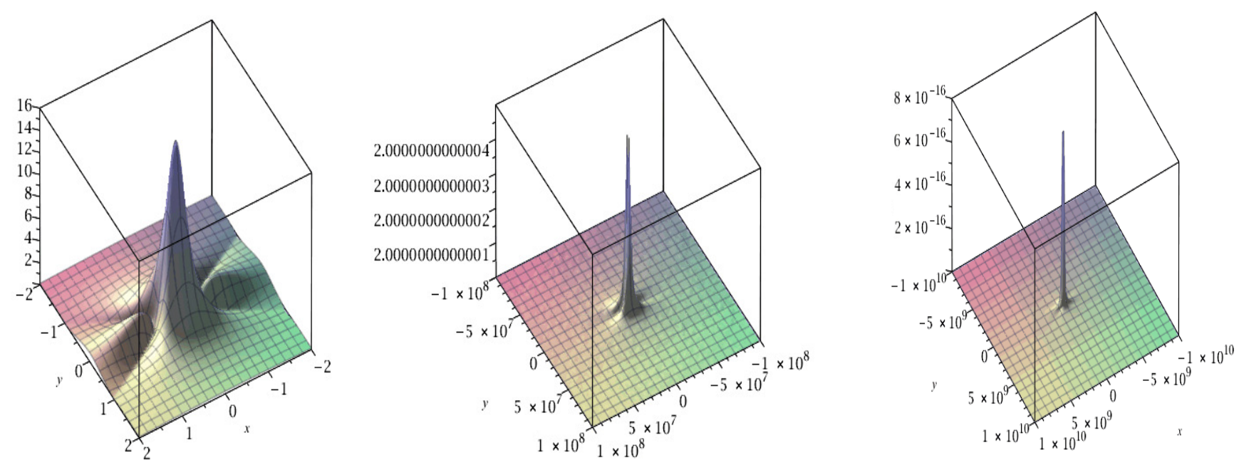
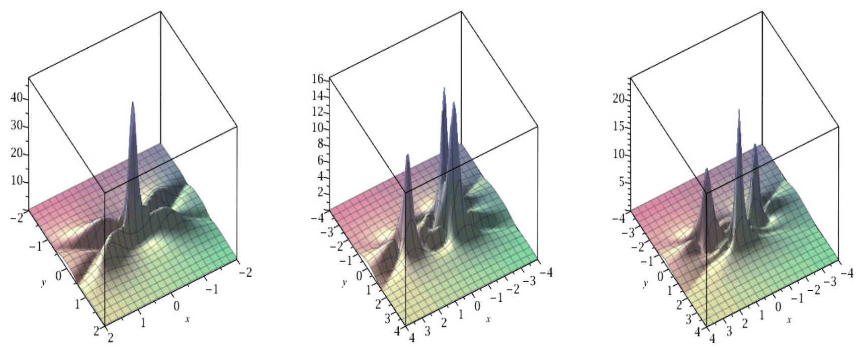
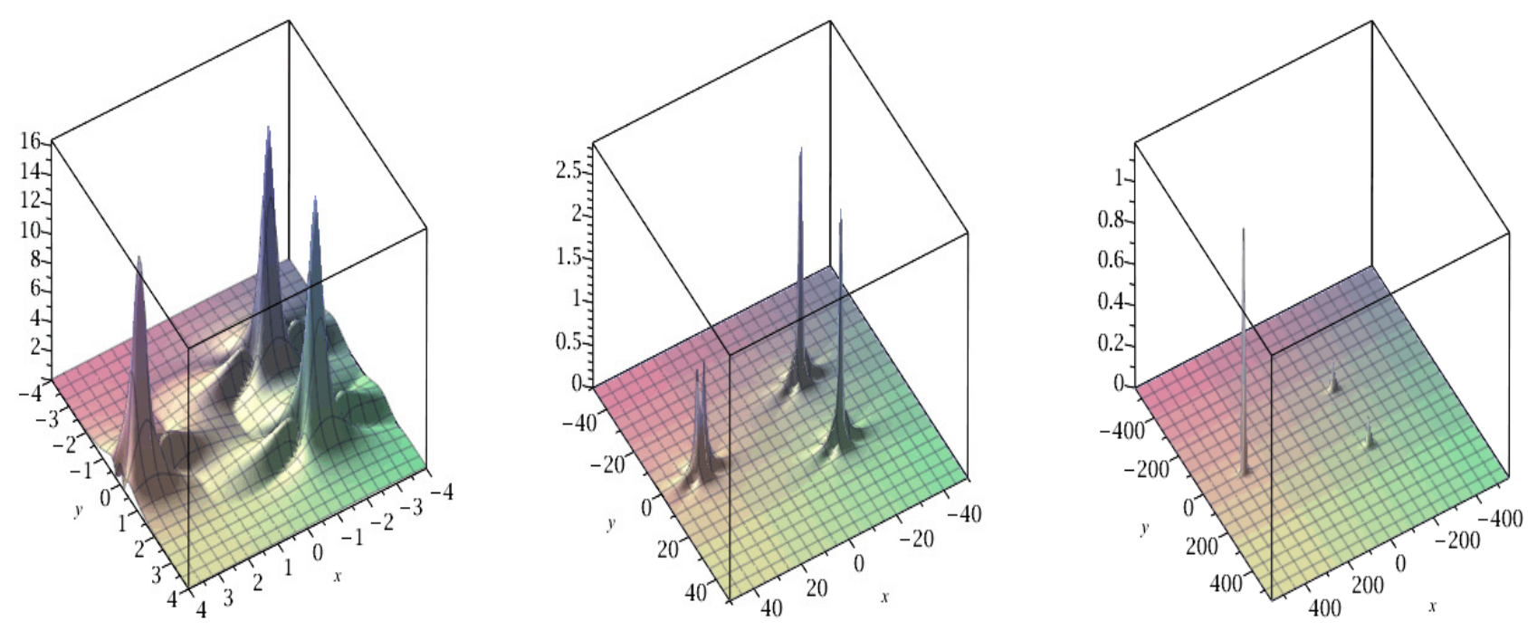
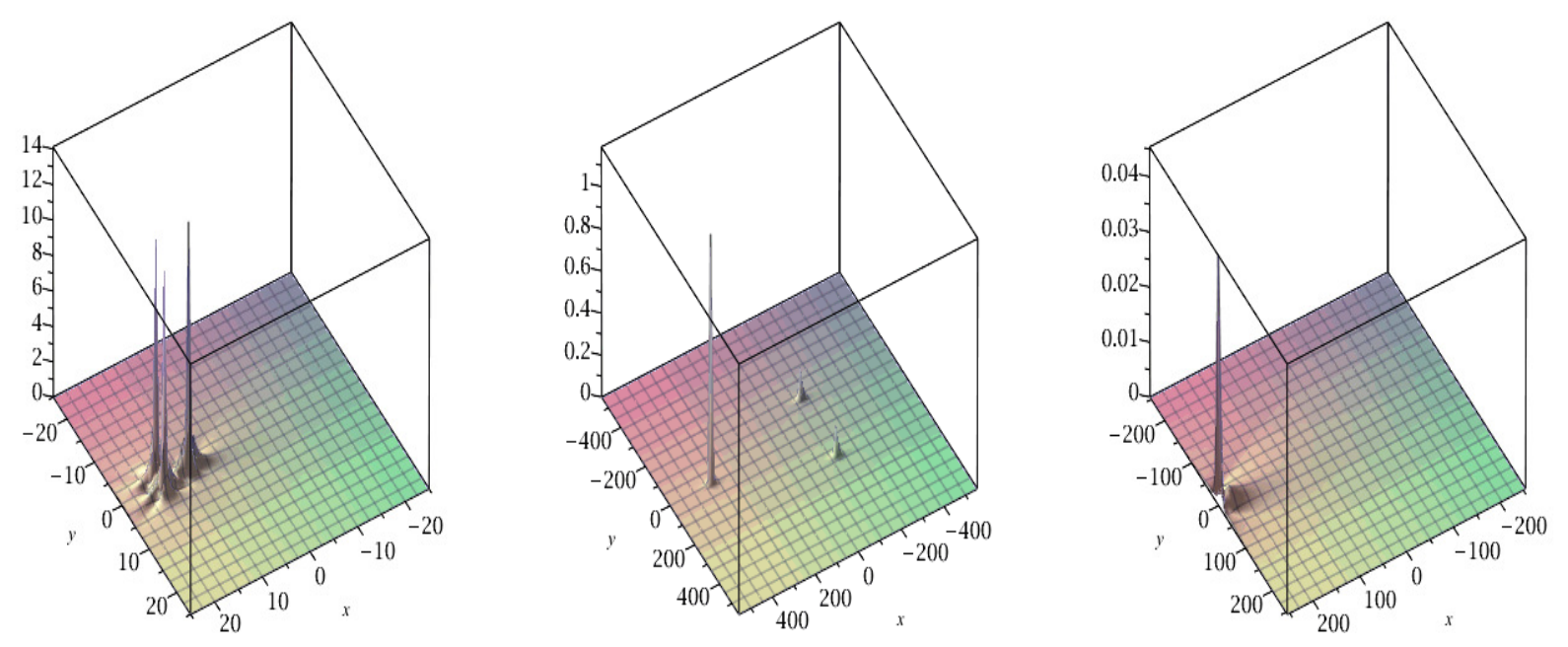
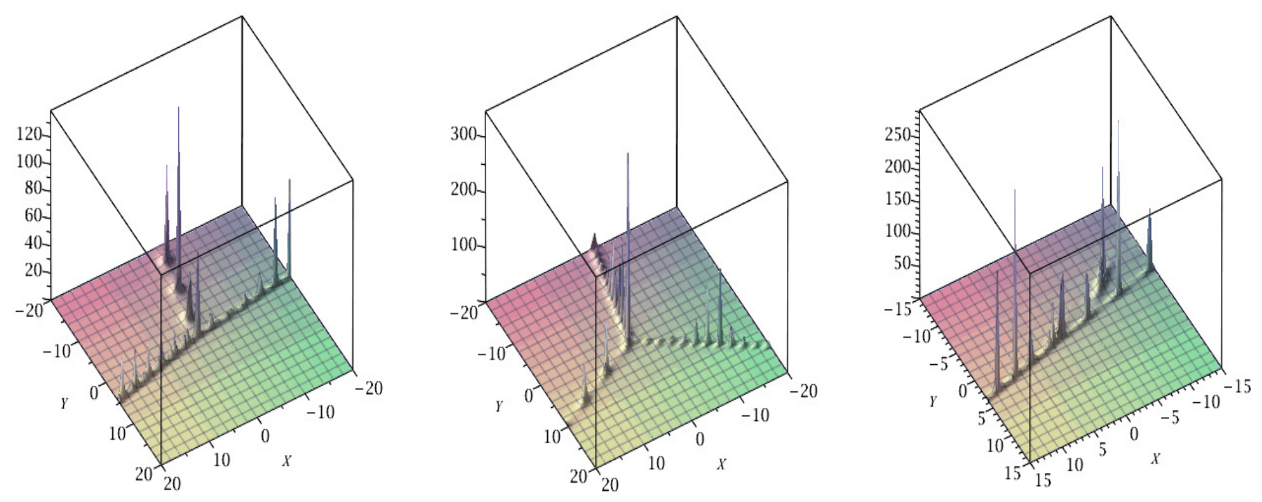
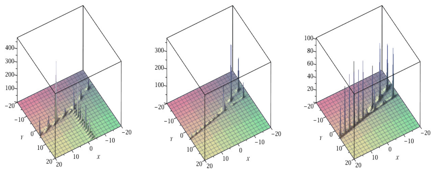
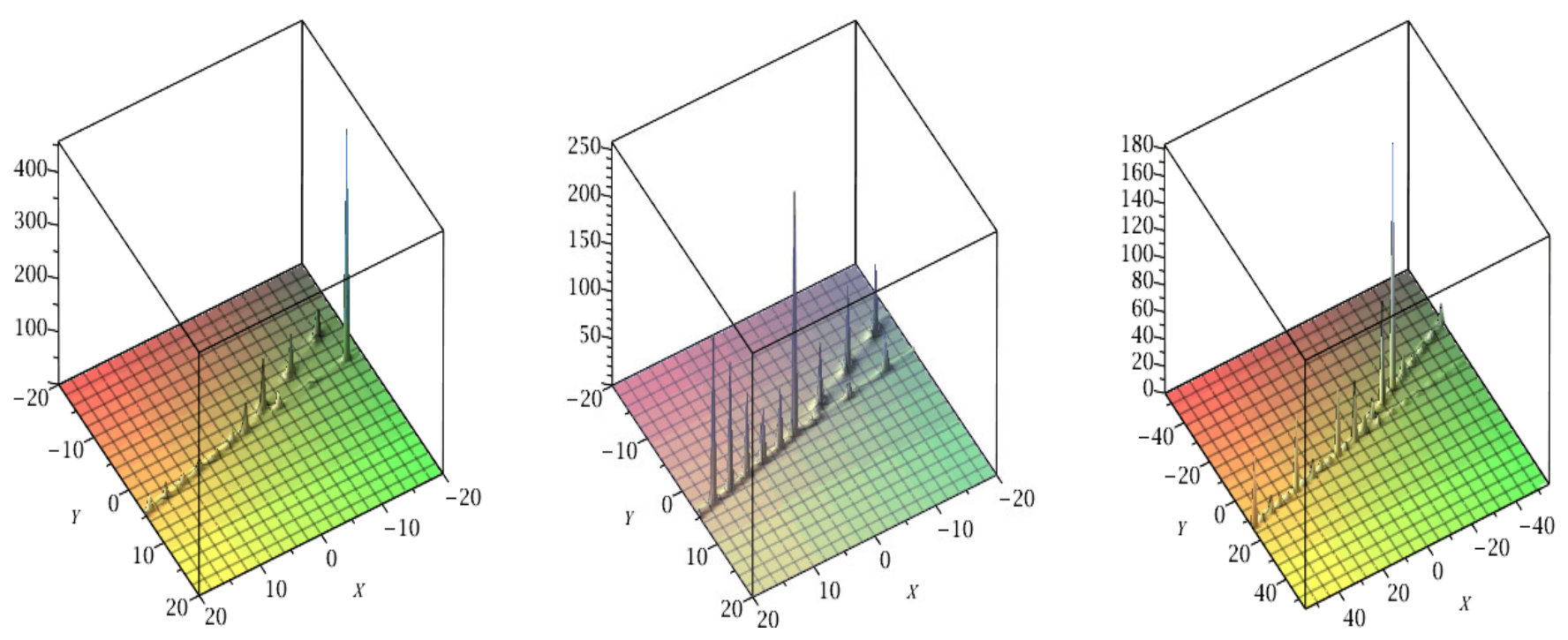
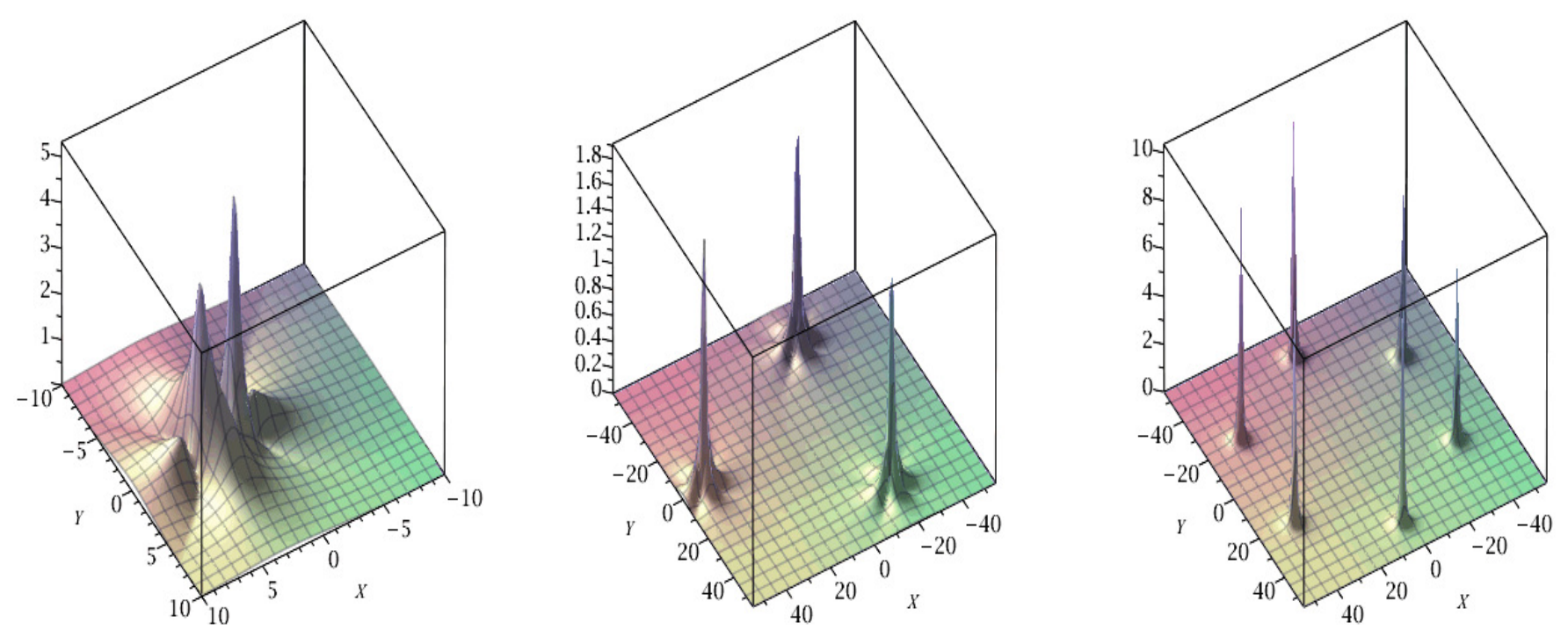
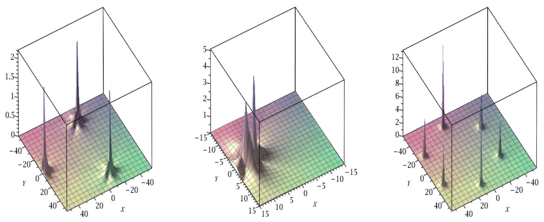
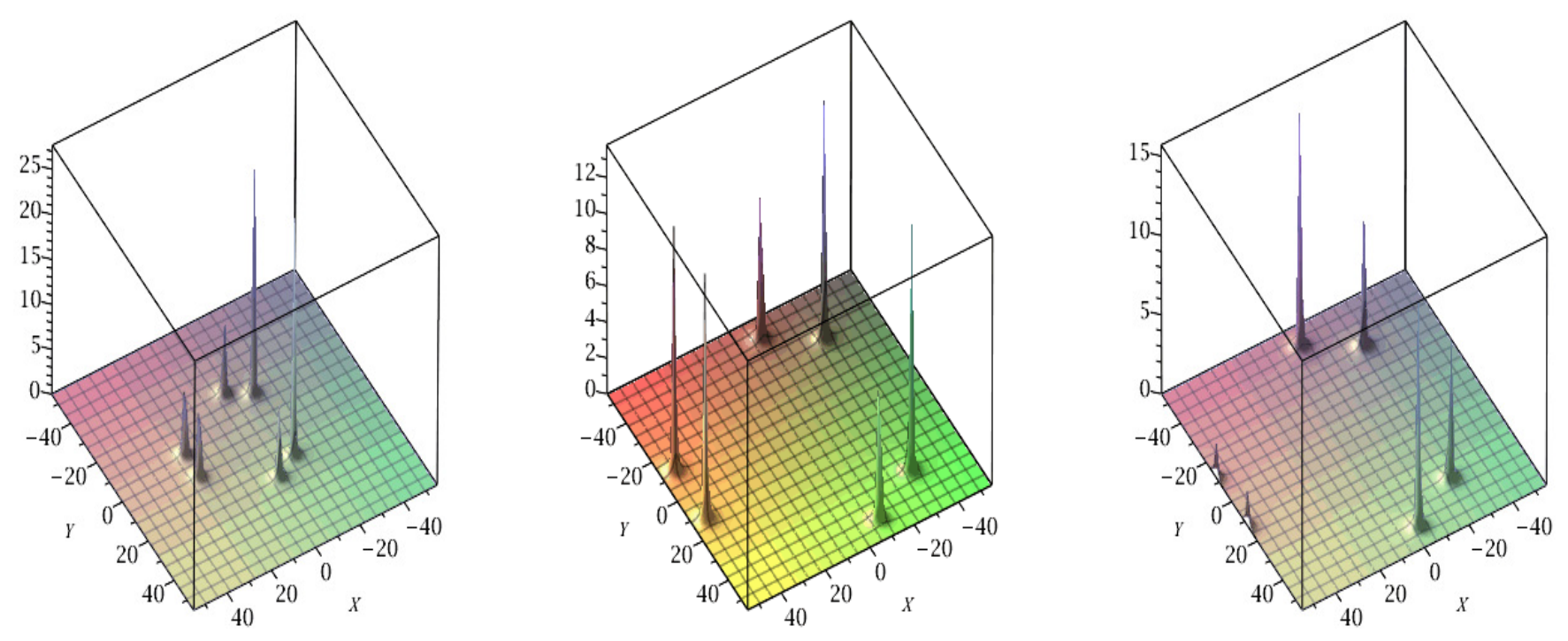
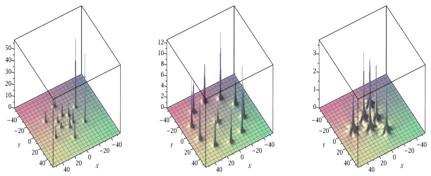
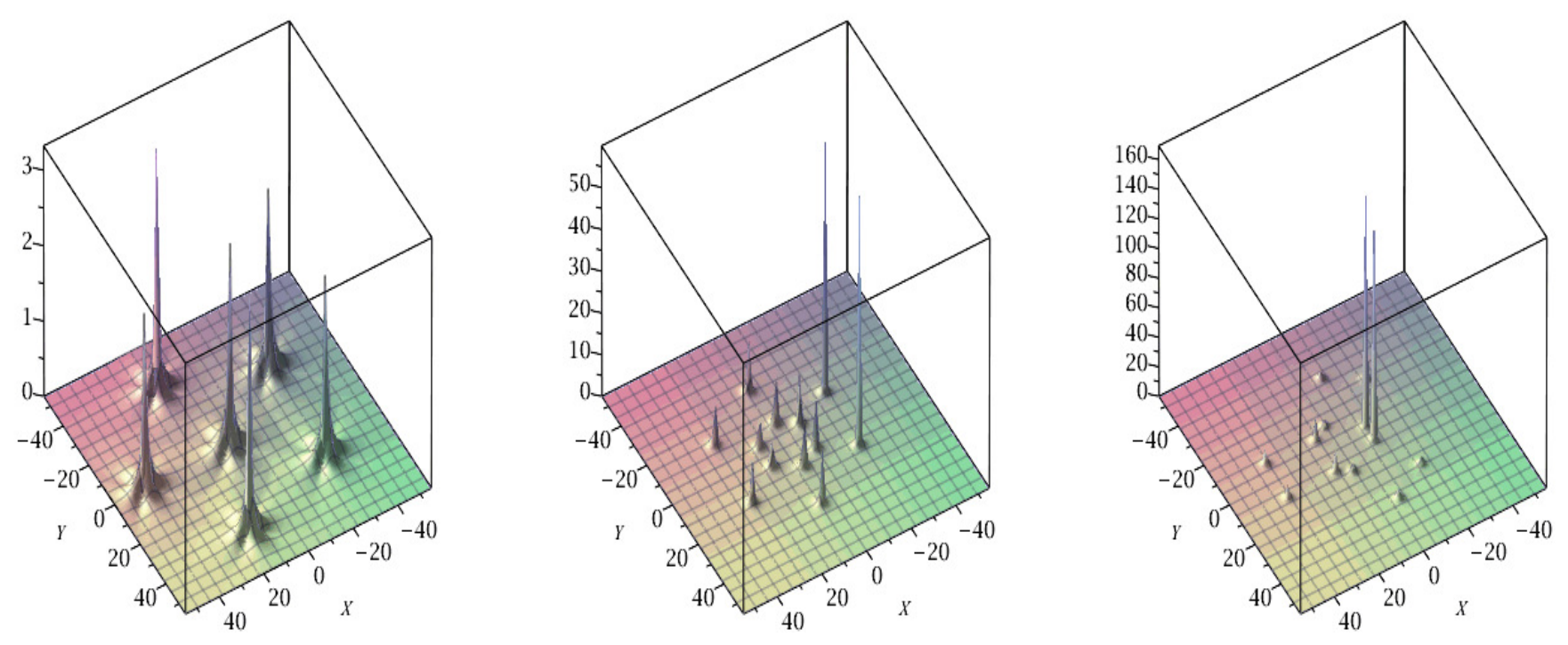
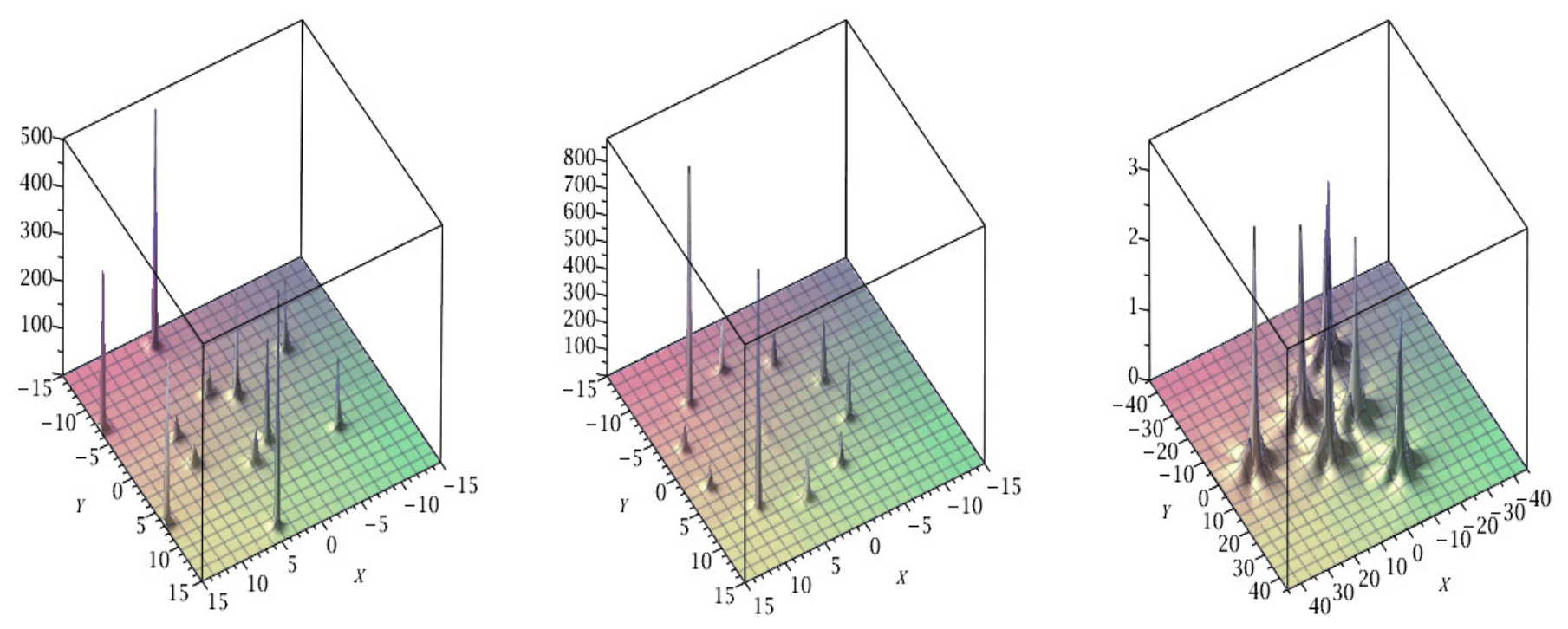
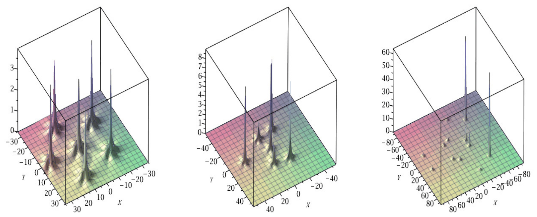
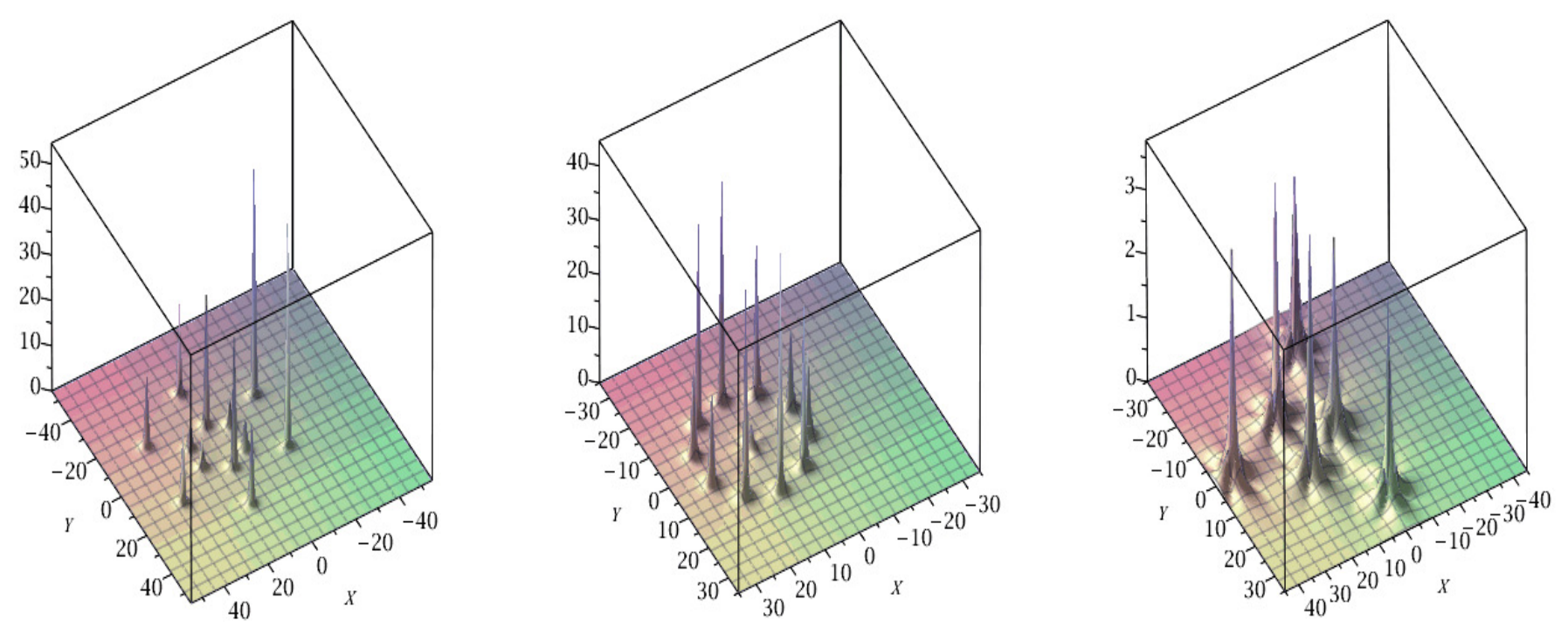
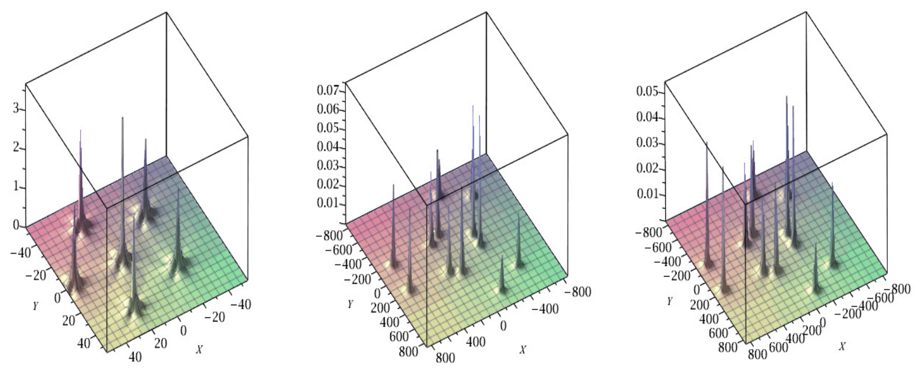
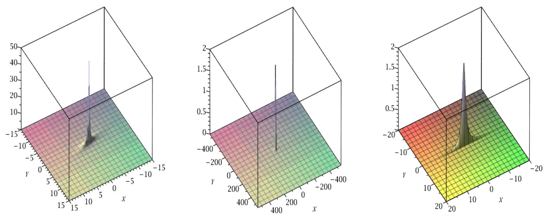
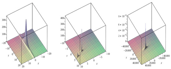
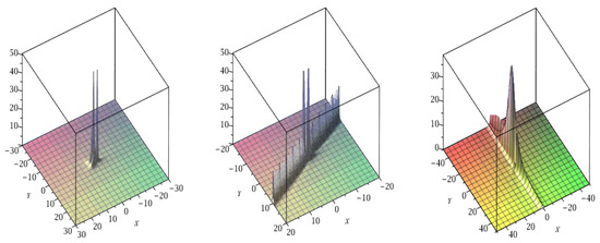
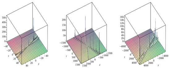
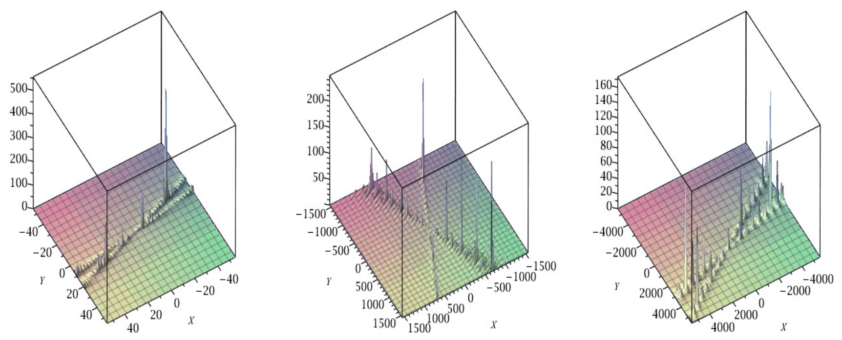
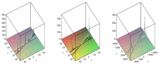
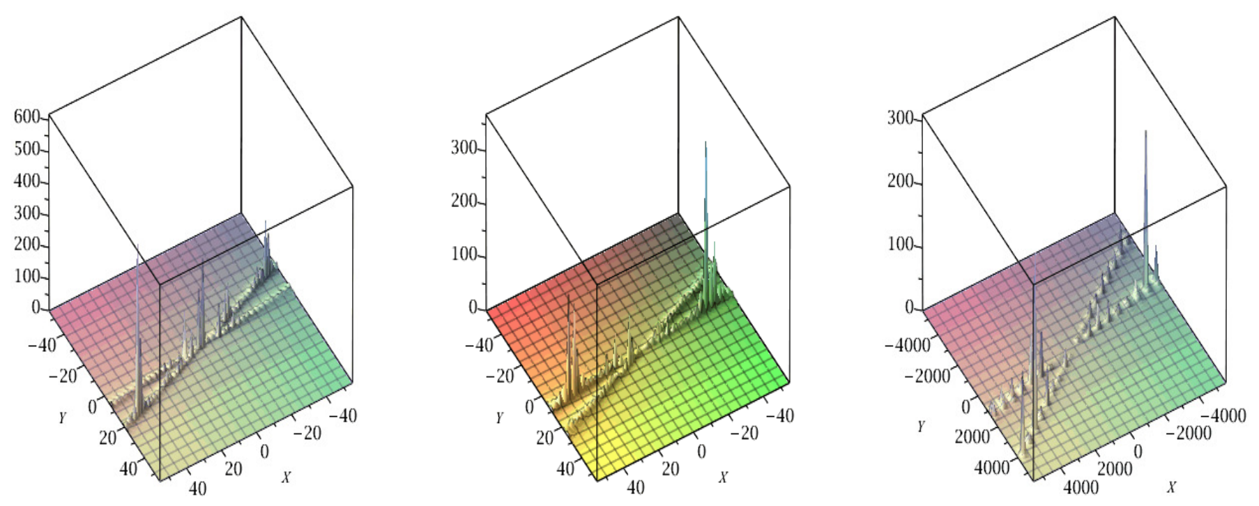
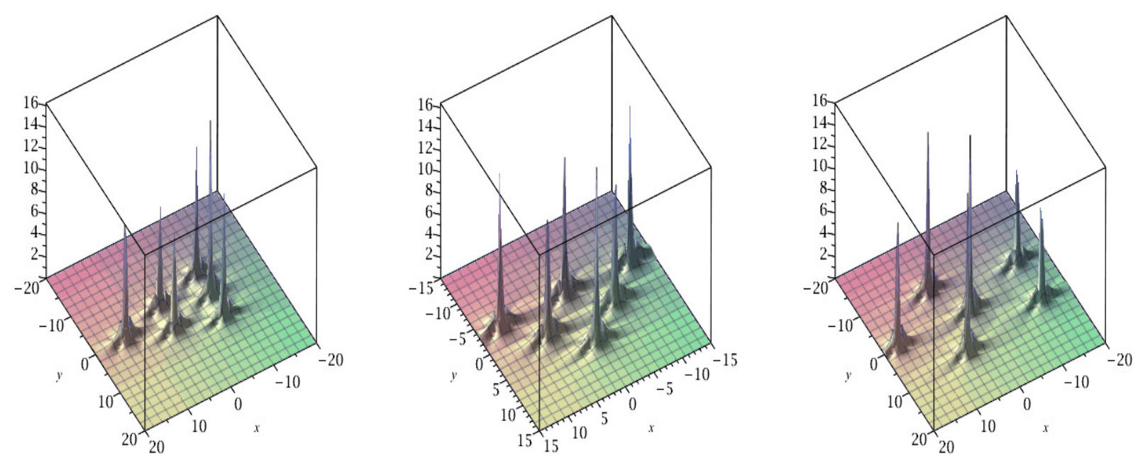
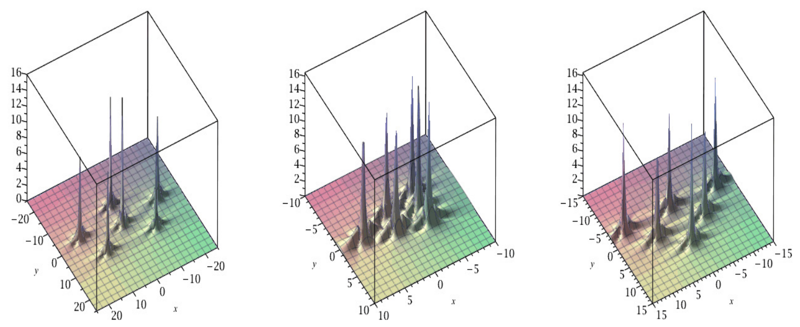
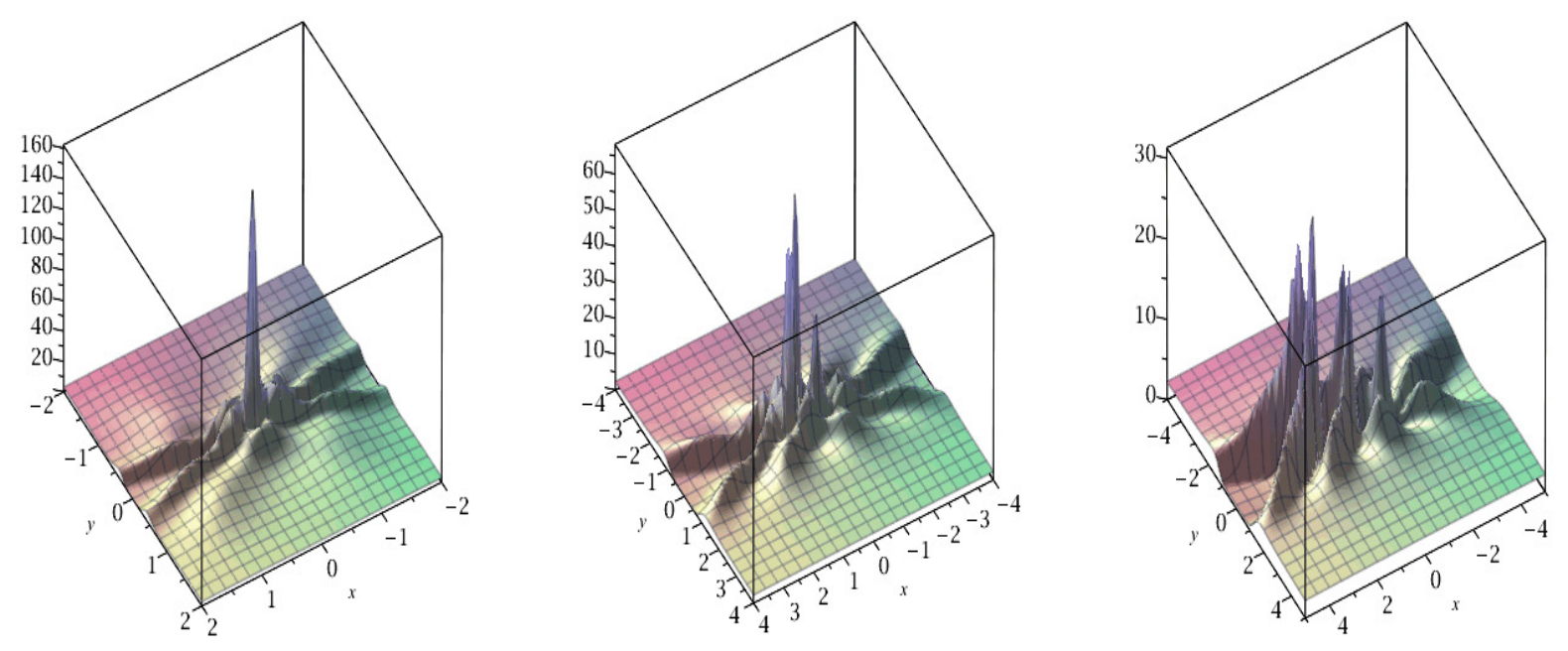
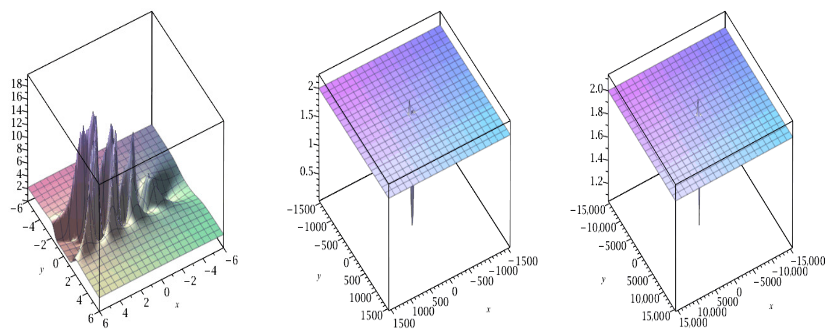
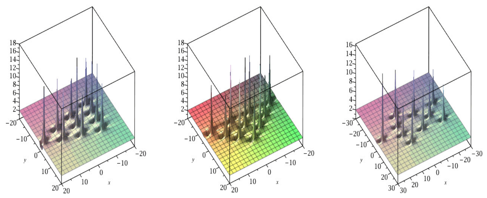
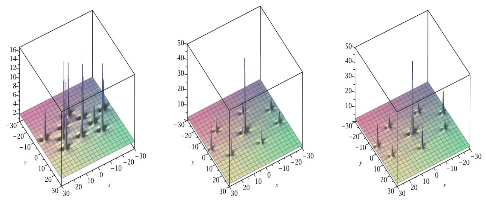
In the following, we only give patterns of the modulus of the solutions in the ( x , y ) plane of coordinates (Figure 1, Figure 2, Figure 3, Figure 4, Figure 5, Figure 6, Figure 7, Figure 8, Figure 9, Figure 10, Figure 11, Figure 12, Figure 13, Figure 14, Figure 15, Figure 16 and Figure 17) as a function of the parameters a i and b i , for 1 i N 1 and for 2 N 3 , and time t.
With this approach, we get regular solutions. In the ( x , y ) plane of coordinates, for a given time t, we obtain configurations in the form of triangles or concentric rings. These patterns are related to the roots of the Vorobev–Yablonski and Ummemura polynomials, as mentioned in [17].

2.7.1. Case N = 1

  • First-order solution.
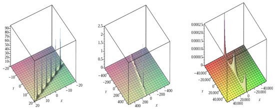
Figure 1. Solution of order 1 to the KP equation for t = 0 (left); for t = 10 4 (center); for t = 10 8 (right).
Axioms 15 00586 g001

2.7.2. Case N = 2

  • Second-order solutions.
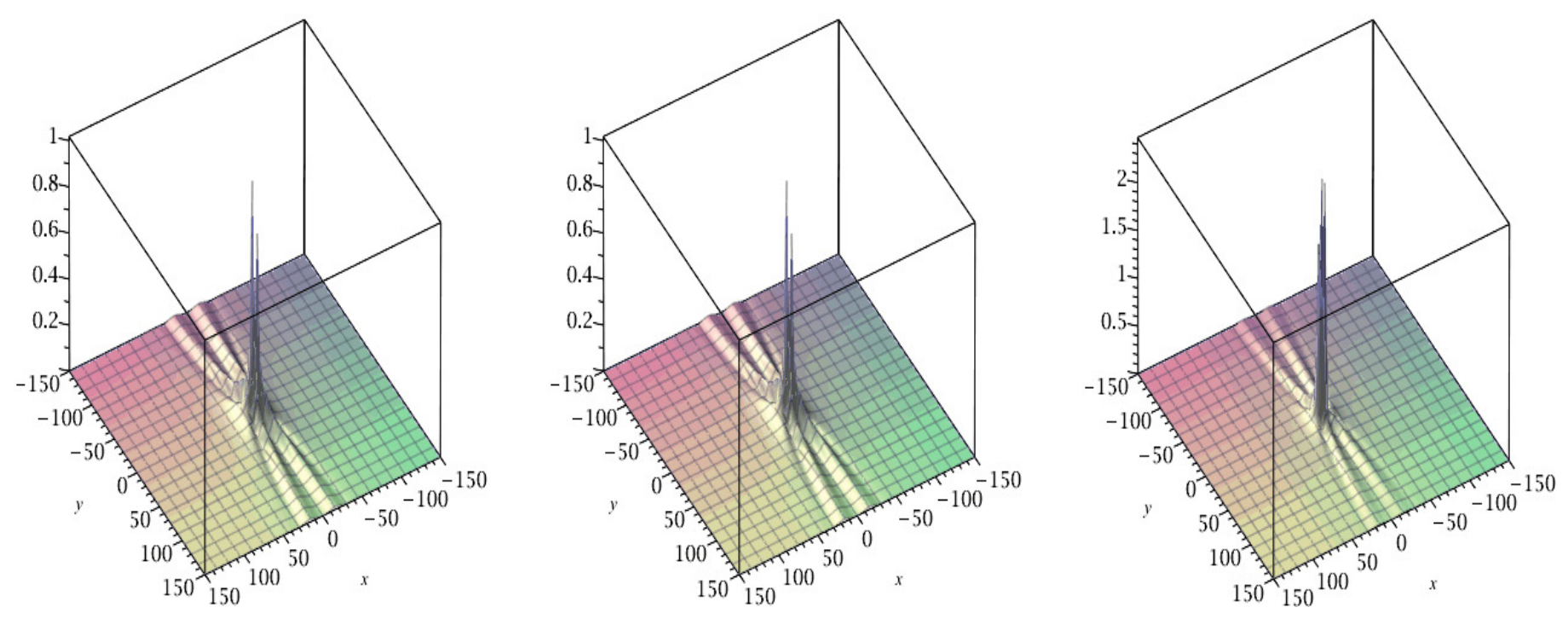
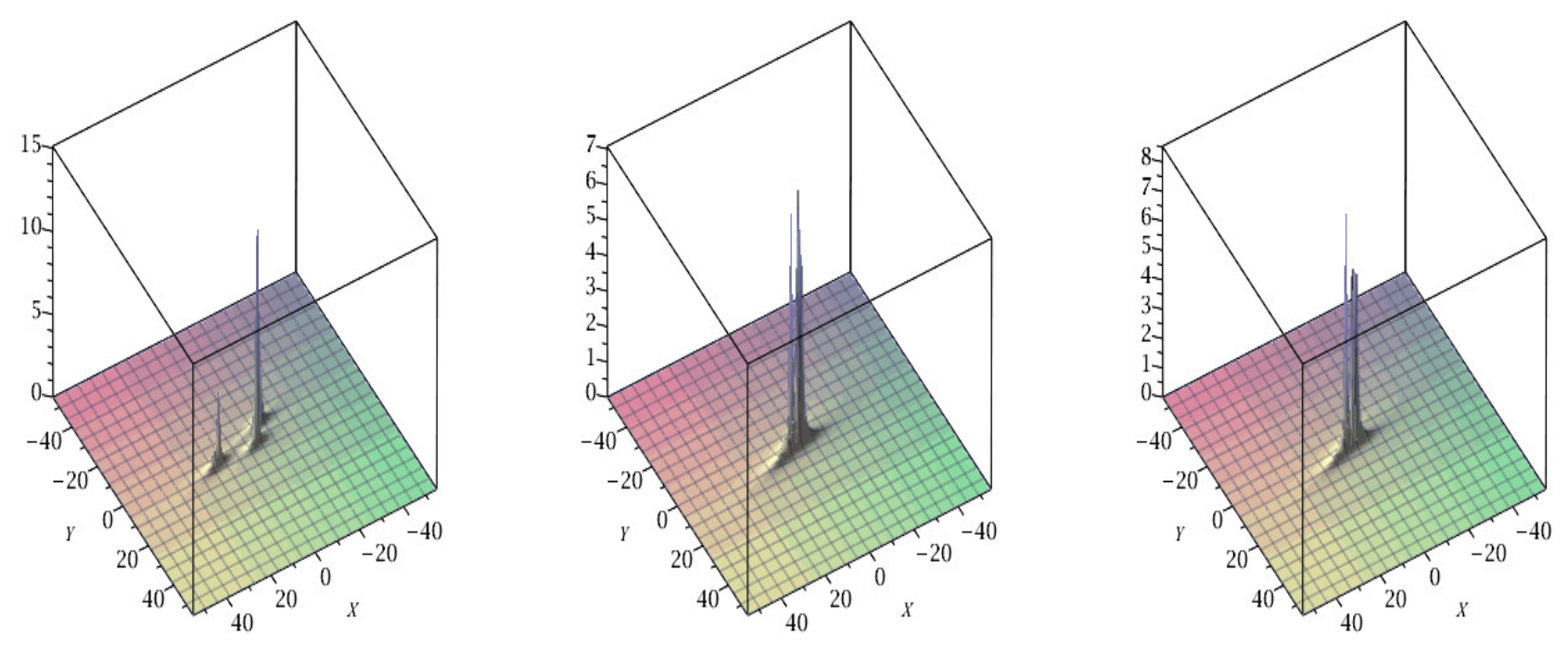
Figure 2. Solutions of order 2 to the KP equation for t = 0 (left); for a 1 = 10 , b 1 = 0 (center); for a 1 = 0 , b 1 = 10 (right).
Axioms 15 00586 g002
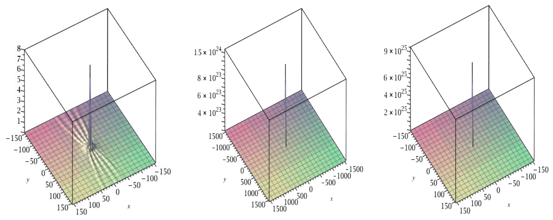
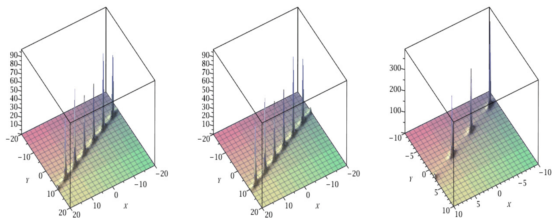
Figure 3. Solutions of order 2 to the KP equation for t = 0 , a 1 = 10 2 , b 1 = 0 (left); t = 0 , a 1 = 10 4 , b 1 = 0 (center); t = 10 , a 1 = 10 8 , b 1 = 0 (right).
Axioms 15 00586 g003
Figure 4. Solutions of order 2 to the KP equation for t = 5 , a 1 = 0 , b 1 = 0 (left); t = 10 , a 1 = 0 , b 1 = 0 (center); t = 100 , a 1 = 0 , b 1 = 0 (right).
Axioms 15 00586 g004

2.7.3. Case N = 3

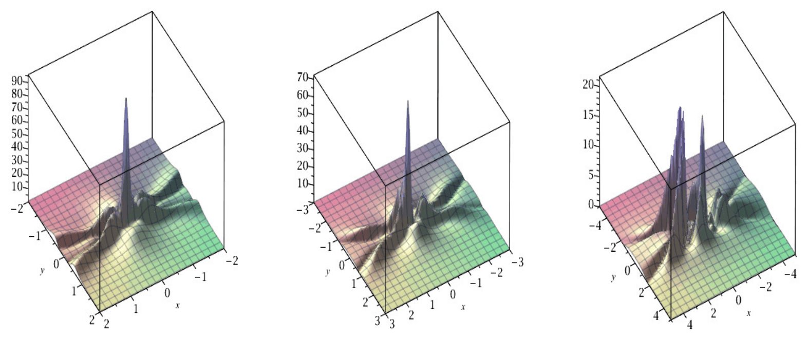
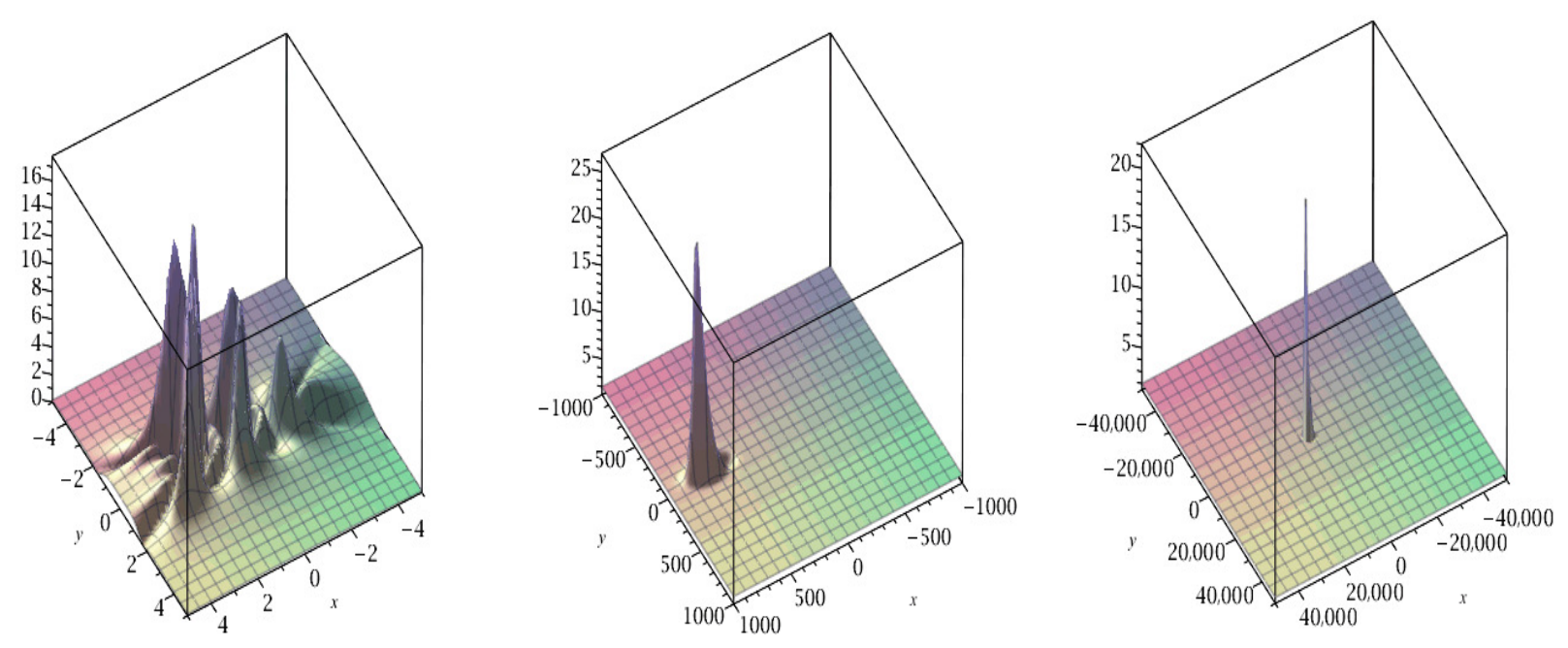
  • Third-order solutions.
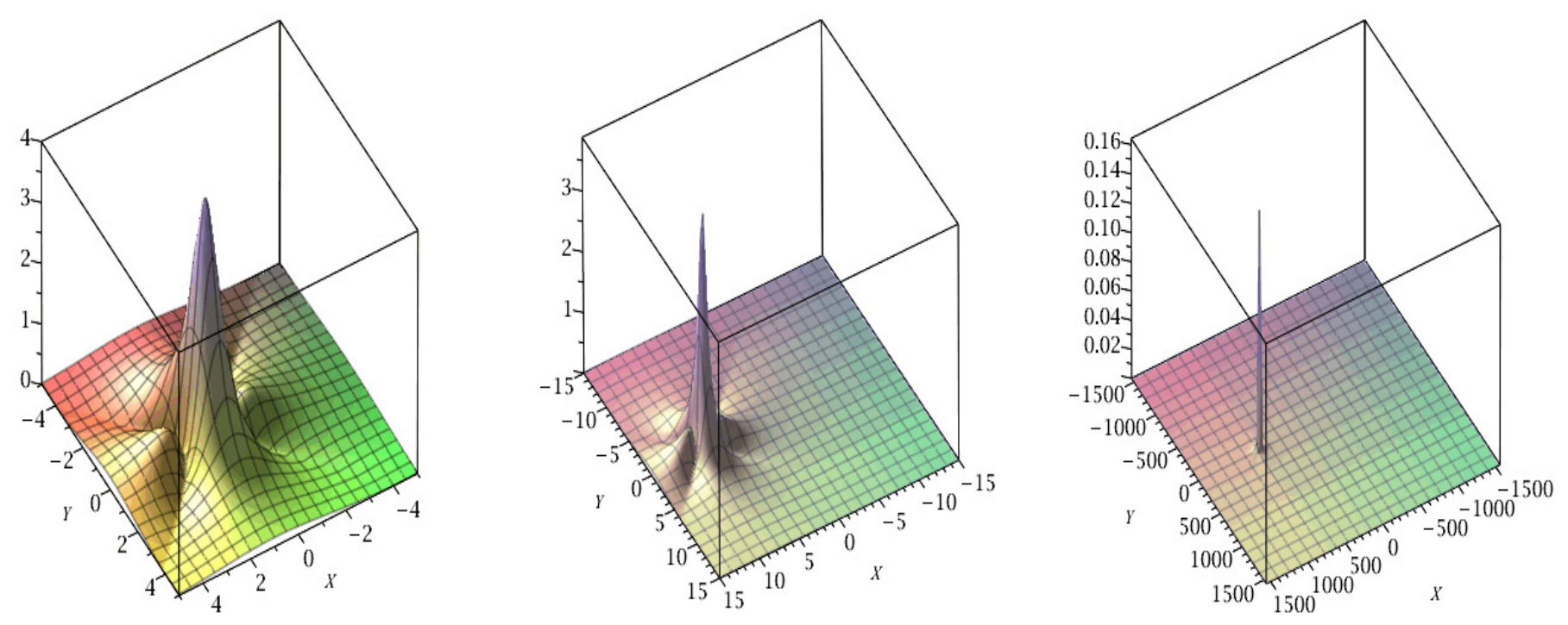
Figure 5. Solutions of order 3 to the KP equation for t = 0 (left); t = 0 , 01 (center); t = 0 , 1 (right). All other parameters are equal to 0.
Axioms 15 00586 g005
Figure 6. Solution of order 3 to the KP equation for t = 0 , 2 (left); t = 10 2 (center); t = 10 3 (right). All other parameters are equal to 0.
Axioms 15 00586 g006
Figure 7. Solutions of order 3 to the KP equation for a 1 = 10 3 (left); b 1 = 10 3 (center); a 2 = 10 6 , t = 0 (right). All other parameters are equal to 0.
Axioms 15 00586 g007
Figure 8. Solutions of order 3 to the KP equation for t = 0 , b 2 = 10 6 (left); t = 0 , 01 , a 1 = 10 3 (center); t = 0 , 1 , b 1 = 10 3 (right). All other parameters are equal to 0.
Axioms 15 00586 g008

2.7.4. Case N = 4

  • Fourth-order solutions.
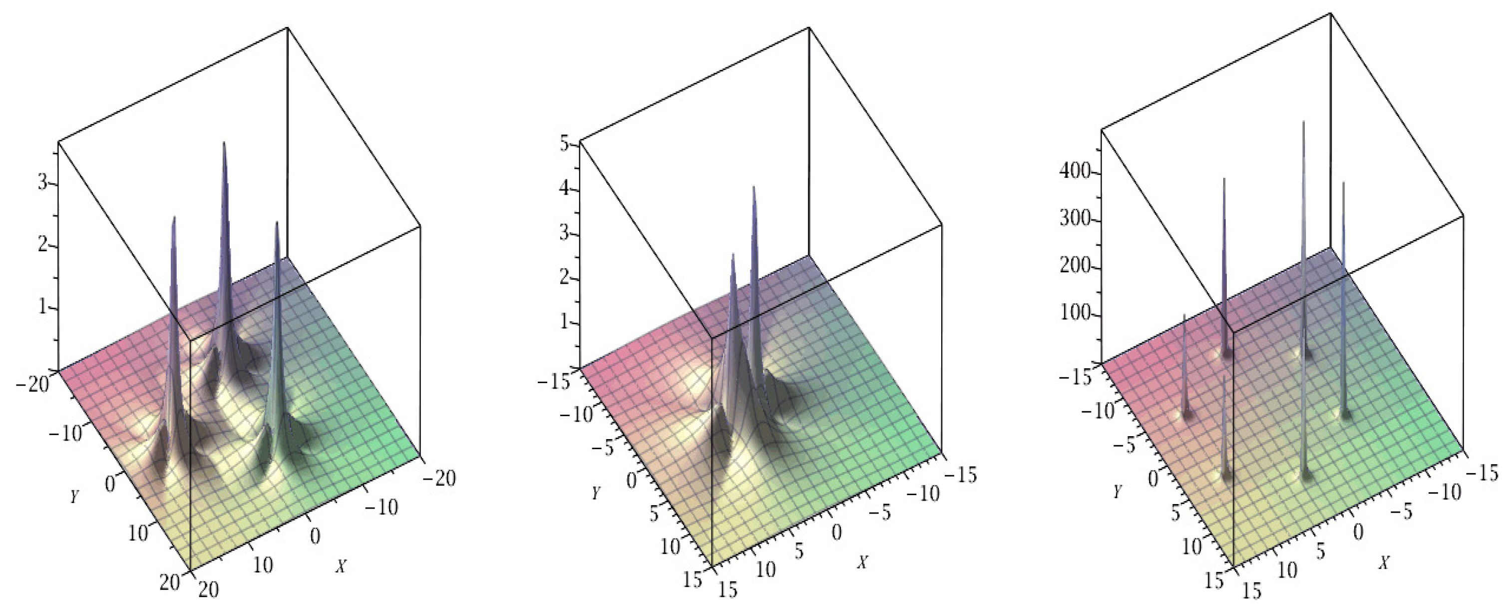
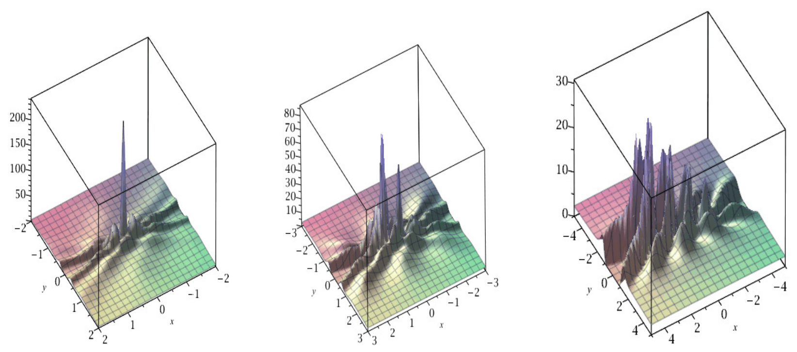
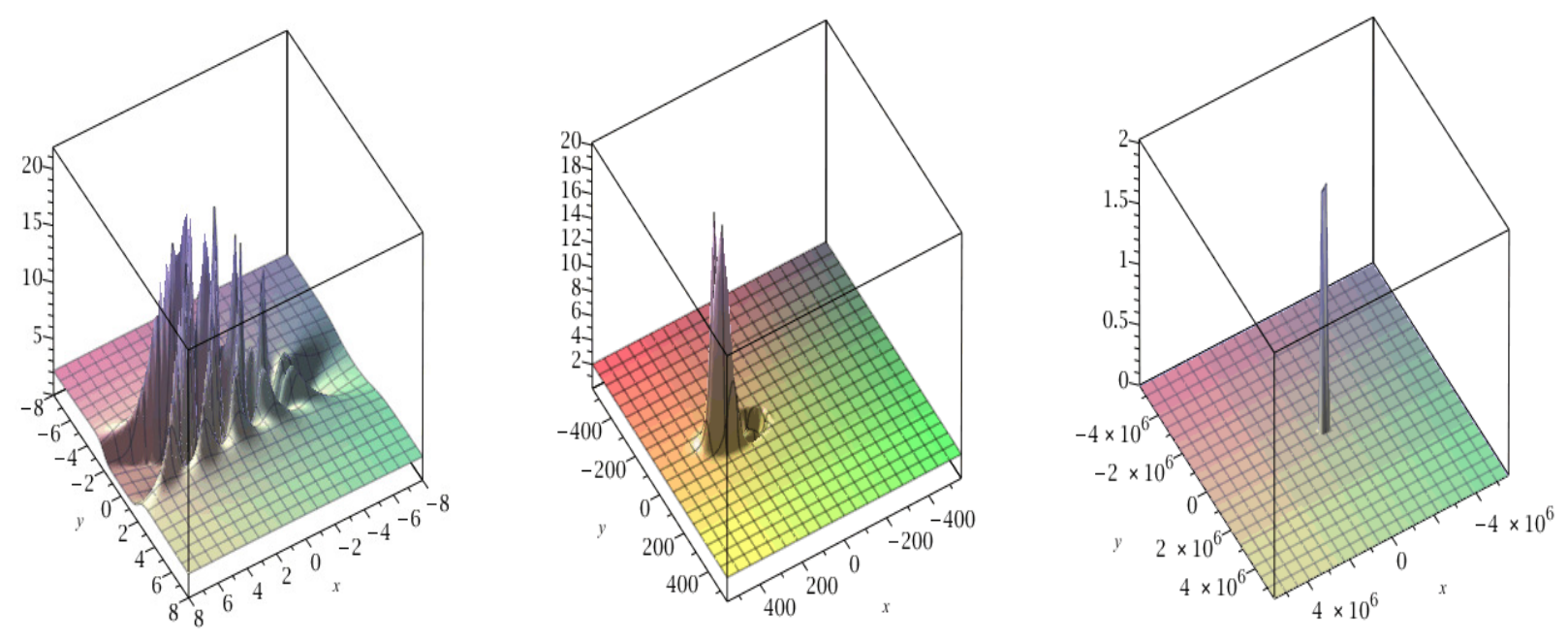
Figure 9. Solution of order 4 to the KP equation for t = 0 (left); t = 0 , 01 (center); t = 0 , 1 (right). All other parameters are equal to 0.
Axioms 15 00586 g009
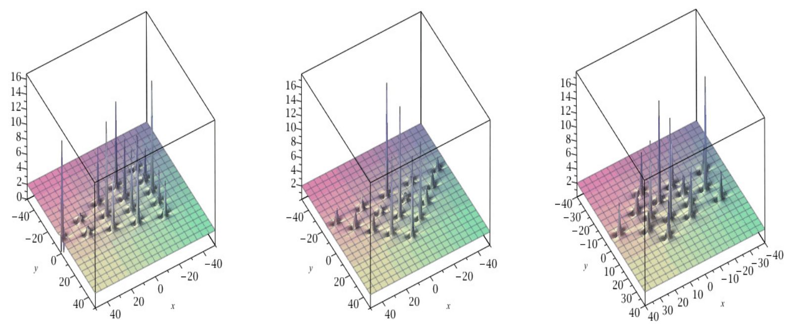
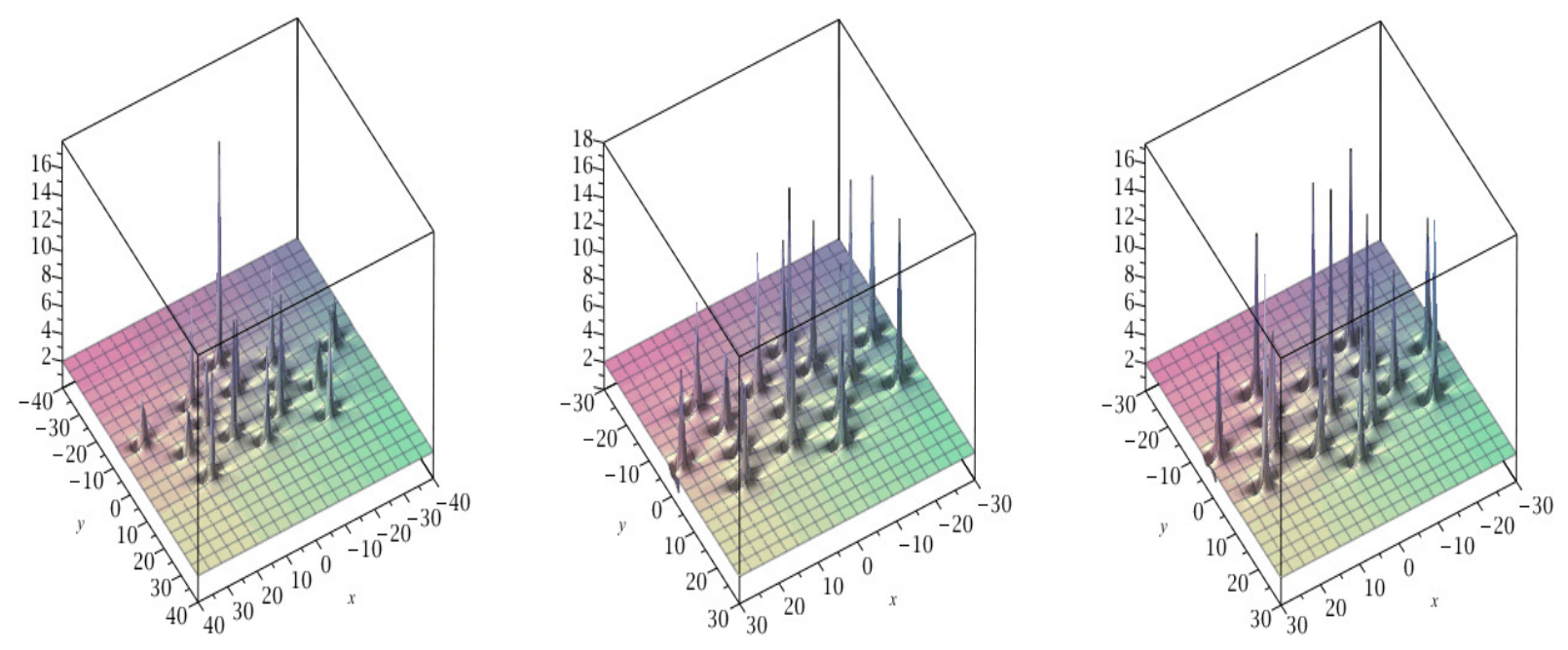
Figure 10. Solution of order 4 to the KP equation for t = 0 , 2 (left); t = 10 (center); t = 50 (right). All other parameters are equal to 0.
Axioms 15 00586 g010
Figure 11. Solutions of order 4 to the KP equation for t = 0 and a 1 = 10 3 (left); b 1 = 10 3 (center); a 2 = 10 6 (right). All other parameters are equal to 0.
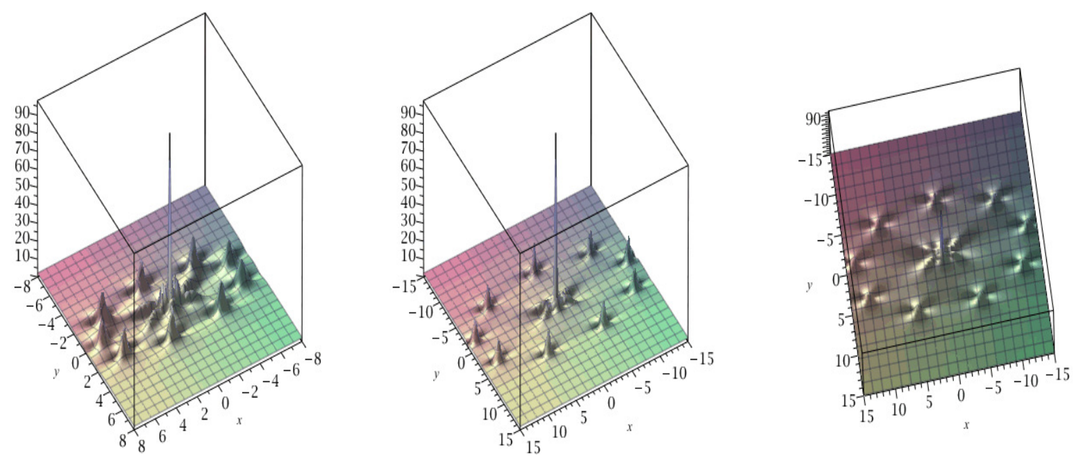
Axioms 15 00586 g011
Figure 12. Solutions of order 4 to the KP equation for t = 0 and b 2 = 10 6 (left); a 3 = 10 9 (center); b 3 = 10 9 (right). All other parameters are equal to 0.
Axioms 15 00586 g012

2.7.5. Case N = 5

  • Fifth-order solutions.
Figure 13. Solutions of order 5 to the KP equation for t = 0 (left); t = 0 , 01 (center); t = 0 , 1 (right). All other parameters are equal to 0.
Axioms 15 00586 g013
Figure 14. Solution of order 5 to the KP equation for t = 0 , 2 (left); t = 20 (center); t = 50 (right). All other parameters are equal to 0.
Axioms 15 00586 g014
Figure 15. Solutions of order 5 to the KP equation for t = 0 and a 1 = 10 4 (left); b 1 = 10 4 (center); a 2 = 10 6 (right). All other parameters are equal to 0.
Axioms 15 00586 g015
Figure 16. Solutions of order 5 to the KP equation for t = 0 and b 2 = 10 6 (left); a 3 = 10 8 (center); b 3 = 10 8 (right). All other parameters are equal to 0.
Axioms 15 00586 g016
Figure 17. Solutions of order 5 to the KP equation for t = 0 and a 4 = 10 8 (left); b 4 = 10 8 (center); b 4 = 10 8 , top view (right). All other parameters are equal to 0.
Axioms 15 00586 g017

2.8. Explicit Expressions of the Solutions

The solutions become very long as the order N increases. We limit ourselves to presenting explicit solutions for orders N = 1 and N = 2 with parameters and N = 3 without parameters.

2.8.1. Case of Order 1

The rational solutions of order 1 to the KP equation can be written as
v ( x , y , t ) = 2 | n ( x , y , t ) | 2 ( d ( x , y , t ) ) 2
with
n ( x , y , t ) = 16 y 2 + 4 x 2 48 x t + 144 t 2 16 i y 3
and
d ( x , y , t ) = 1 + 4 x 2 + 144 t 2 + 16 y 2 48 x t ,
The representations of the solutions can be seen in Figure 1.

2.8.2. Case of Order 2

The rational solutions of order 2 to the KP equation depending on two real parameters can be written as
v ( x , y , t ) = 2 | n ( x , y , t ) | 2 ( d ( x , y , t ) ) 2
with
n ( x , y , t ) = 45 1728 x t 2 a 1 + 288 x 2 t a 1 18432 x 3 t y 2 + 165888 x 2 t 2 y 2 663552 x t 3 y 2 + 192 x a 1 y 2 1152 t a 1 y 2 36864 x t y 4 + 96 b 1 x 2 y + 3456 b 1 t 2 y + 4096 y 6 + b 1 2 + a 1 2 + 2985984 t 6 + 64 x 6 8448 y 4 518400 t 4 144 x 4 180 x 2 18000 t 2 + 3456 t 3 a 1 16 x 3 a 1 2985984 t 5 x 2304 x 5 t + 1244160 t 4 x 2 + 34560 x 4 t 2 276480 x 3 t 3 128 b 1 y 3 + 3072 x 2 y 4 + 110592 t 2 y 4 + 995328 t 4 y 2 + 768 x 4 y 2 + 4992 x 3 t 58752 x 2 t 2 + 290304 x t 3 + 24 b 1 y 5760 x 2 y 2 96768 t 2 y 2 36 x a 1 + 24 t a 1 + 5616 x t 1872 y 2 + 50688 x t y 2 1152 b 1 x t y 48 i b 1 x 2 192 i x y a 1 + 576 i x b 1 t + 720 i y 12288 i y 5 1536 i y 3 + 4608 i t y x + 73728 i y 3 x t + 18432 i x 3 y t + 663552 i t 3 y x 165888 i x 2 t 2 y 12 i b 1 + 192 i y 2 b 1 1728 i b 1 t 2 + 1152 i y t a 1 995328 i t 4 y 768 i x 4 y 69120 i t 2 y 221184 i t 2 y 3 + 1152 i x 2 y 6144 i x 2 y 3
d ( x , y , t ) = 9 1728 x t 2 a 1 + 288 x 2 t a 1 18432 x 3 t y 2 + 165888 x 2 t 2 y 2 663552 x t 3 y 2 + 192 x a 1 y 2 1152 t a 1 y 2 36864 x t y 4 + 96 b 1 x 2 y + 3456 b 1 t 2 y + 4096 y 6 + b 1 2 + a 1 2 + 2985984 t 6 + 64 x 6 + 6912 y 4 269568 t 4 + 48 x 4 + 108 x 2 + 20016 t 2 + 3456 t 3 a 1 16 x 3 a 1 2985984 t 5 x 2304 x 5 t + 1244160 t 4 x 2 + 34560 x 4 t 2 276480 x 3 t 3 128 b 1 y 3 + 3072 x 2 y 4 + 110592 t 2 y 4 + 995328 t 4 y 2 + 768 x 4 y 2 + 384 x 3 t 17280 x 2 t 2 + 124416 x t 3 72 b 1 y 1152 x 2 y 2 + 69120 t 2 y 2 + 12 x a 1 264 t a 1 2448 x t + 1584 y 2 4608 x t y 2 1152 b 1 x t y
The representations of the solutions can be seen in Figure 2, Figure 3 and Figure 4.

2.8.3. Case of Order 3

The rational solutions depending on four parameters are too long; only rational solutions without parameters are presented; they can be written as
v ( x , y , t ) = 2 | n ( x , y , t ) | 2 ( d ( x , y , t ) ) 2
with
n ( x , y , t ) d ( x , y , t ) = F ( 2 x , 4 y , 4 t ) i H ( 2 x , 4 y , 4 t ) Q ( 2 x , 4 y , 4 t )
and
F ( X , Y , T ) = k = 0 12 f k ( Y , T ) X k , H ( X , Y , T ) = k = 0 12 h k ( Y , T ) X k , Q ( X , Y , T ) = k = 0 12 q k ( Y , T ) X k .
f 12 = 1 , f 11 = 36 T , f 10 = 594 T 2 + 6 Y 2 18 , f 9 = 5940 T 3 + ( 180 Y 2 + 780 ) T , f 8 = 40095 T 4 + 15 Y 4 + ( 2430 Y 2 13770 ) T 2 450 Y 2 225 , f 7 = 192456 T 5 + ( 19440 Y 2 + 136080 ) T 3 + ( 360 Y 4 + 10800 Y 2 + 5400 ) T , f 6 = 673596 T 6 + 20 Y 6 + ( 102060 Y 2 850500 ) T 4 1380 Y 4 + ( 3780 Y 4 113400 Y 2 48060 ) T 2 + 1980 Y 2 2700 f 5 = 1732104 T 7 + ( 367416 Y 2 + 3551688 ) T 5 + ( 22680 Y 4 + 680400 Y 2 + 184680 ) T 3 + ( 360 Y 6 + 23400 Y 4 + 7560 Y 2 + 70200 ) T , f 4 = 3247695 T 8 + 15 Y 8 + ( 918540 Y 2 10103940 ) T 6 1620 Y 6 + ( 85050 Y 4 2551500 Y 2 109350 ) T 4 + 2250 Y 4 + ( 2700 Y 6 164700 Y 4 251100 Y 2 1077300 ) T 2 + 2700 Y 2 + 14175 , f 3 = 4330260 T 9 + ( 1574640 Y 2 + 19420560 ) T 7 + ( 204120 Y 4 + 6123600 Y 2 1603800 ) T 5 + ( 10800 Y 6 + 615600 Y 4 + 1263600 Y 2 + 7376400 ) T 3 + ( 180 Y 8 + 17520 Y 6 + 1800 Y 4 + 399600 Y 2 429300 ) T , f 2 = 3897234 T 10 + 6 Y 10 + ( 1771470 Y 2 24210090 ) T 8 810 Y 8 + ( 306180 Y 4 9185400 Y 2 + 5904900 ) T 6 + 3420 Y 6 + ( 24300 Y 6 1287900 Y 4 2259900 Y 2 23886900 ) T 4 83700 Y 4 + ( 810 Y 8 70200 Y 6 180900 Y 4 2446200 Y 2 + 3746250 ) T 2 + 287550 Y 2 + 28350 , f 1 = 2125764 T 11 + ( 1180980 Y 2 + 17714700 ) T 9 + ( 262440 Y 4 + 7873200 Y 2 8660520 ) T 7 + ( 29160 Y 6 + 1428840 Y 4 + 612360 Y 2 + 36012600 ) T 5 + ( 1620 Y 8 + 123120 Y 6 + 793800 Y 4 + 5670000 Y 2 18638100 ) T 3 + ( 36 Y 10 + 4140 Y 8 + 57240 Y 6 + 394200 Y 4 1854900 Y 2 850500 ) T , f 0 = 531441 T 12 + Y 12 + ( 354294 Y 2 5786802 ) T 10 138 Y 10 + ( 98415 Y 4 2952450 Y 2 + 4822335 ) T 8 8145 Y 8 + ( 14580 Y 6 656100 Y 4 + 1443420 Y 2 20047500 ) T 6 37260 Y 6 + ( 1215 Y 8 79380 Y 6 984150 Y 4 6002100 Y 2 + 40935375 ) T 4 + 327375 Y 4 + ( 54 Y 10 5130 Y 8 182340 Y 6 1509300 Y 4 + 3106350 Y 2 + 1129950 ) T 2 + 141750 Y 2 14175 .
h 12 = 0 , h 11 = 0 , h 10 = 24 Y , h 9 = 720 T Y , h 8 = 9720 T 2 Y + 120 Y 3 360 Y , h 7 = 77760 T 3 Y + ( 2880 Y 3 + 8640 Y ) T , h 6 = 408240 T 4 Y + 240 Y 5 3360 Y 3 + ( 30240 Y 3 90720 Y ) T 2 3600 Y , h 5 = 1469664 T 5 Y + ( 181440 Y 3 + 544320 Y ) T 3 + ( 4320 Y 5 + 48960 Y 3 + 99360 Y ) T , h 4 = 3674160 T 6 Y + 240 Y 7 5040 Y 5 + ( 680400 Y 3 2041200 Y ) T 4 10800 Y 3 + ( 32400 Y 5 280800 Y 3 486000 Y ) T 2 32400 Y h 3 = 6298560 T 7 Y + ( 1632960 Y 3 + 4898880 Y ) T 5 + ( 129600 Y 5 + 777600 Y 3 1166400 Y ) T 3 + ( 2880 Y 7 + 37440 Y 5 100800 Y 3 + 734400 Y ) T , h 2 = 7085880 T 8 Y + 120 Y 9 1440 Y 7 + ( 2449440 Y 3 7348320 Y ) T 6 + 41040 Y 5 + ( 291600 Y 5 972000 Y 3 + 14288400 Y ) T 4 151200 Y 3 + ( 12960 Y 7 64800 Y 5 + 1144800 Y 3 3823200 Y ) T 2 + 113400 Y , h 1 = 4723920 T 9 Y + ( 2099520 Y 3 + 6298560 Y ) T 7 + ( 349920 Y 5 + 233280 Y 3 36741600 Y ) T 5 + ( 25920 Y 7 77760 Y 5 2980800 Y 3 + 14904000 Y ) T 3 + ( 720 Y 9 2880 Y 7 4320 Y 5 + 1425600 Y 3 + 874800 Y ) T h 0 = 1417176 T 10 Y + 24 Y 11 + 600 Y 9 + ( 787320 Y 3 2361960 Y ) T 8 20880 Y 7 + ( 174960 Y 5 + 349920 Y 3 + 30967920 Y ) T 6 231120 Y 5 + ( 19440 Y 7 + 213840 Y 5 + 2235600 Y 3 27507600 Y ) T 4 59400 Y 3 + ( 1080 Y 9 + 21600 Y 7 114480 Y 5 4644000 Y 3 7273800 Y ) T 2 + 113400 Y .
q 12 = 1 , q 11 = 36 T , q 10 = 594 T 2 + 6 Y 2 + 6 , q 9 = 5940 T 3 + ( 180 Y 2 + 60 ) T , q 8 = 40095 T 4 + 15 Y 4 + ( 2430 Y 2 4050 ) T 2 90 Y 2 + 135 , q 7 = 192456 T 5 + ( 19440 Y 2 + 58320 ) T 3 + ( 360 Y 4 + 2160 Y 2 3240 ) T , q 6 = 673596 T 6 + 20 Y 6 + ( 102060 Y 2 442260 ) T 4 180 Y 4 + ( 3780 Y 4 22680 Y 2 + 42660 ) T 2 + 540 Y 2 + 2340 , q 5 = 1732104 T 7 + ( 367416 Y 2 + 2082024 ) T 5 + ( 22680 Y 4 + 136080 Y 2 359640 ) T 3 + ( 360 Y 6 + 1800 Y 4 1080 Y 2 55080 ) T , q 4 = 3247695 T 8 + 15 Y 8 + ( 918540 Y 2 6429780 ) T 6 + 60 Y 6 + ( 85050 Y 4 510300 Y 2 + 1931850 ) T 4 1350 Y 4 + ( 2700 Y 6 2700 Y 4 + 72900 Y 2 + 639900 ) T 2 + 13500 Y 2 + 3375 , q 3 = 4330260 T 9 + ( 1574640 Y 2 + 13122000 ) T 7 + ( 204120 Y 4 + 1224720 Y 2 6502680 ) T 5 + ( 10800 Y 6 32400 Y 4 1069200 Y 2 4676400 ) T 3 + ( 180 Y 8 2640 Y 6 70200 Y 4 421200 Y 2 + 45900 ) T , q 2 = 3897234 T 10 + 6 Y 10 + ( 1771470 Y 2 17124210 ) T 8 + 270 Y 8 + ( 306180 Y 4 1837080 Y 2 + 13253220 ) T 6 + 13500 Y 6 + ( 24300 Y 6 + 170100 Y 4 + 5321700 Y 2 + 19561500 ) T 4 + 78300 Y 4 + ( 810 Y 8 + 20520 Y 6 + 661500 Y 4 + 3321000 Y 2 984150 ) T 2 36450 Y 2 + 12150 , q 1 = 2125764 T 11 + ( 1180980 Y 2 + 12990780 ) T 9 + ( 262440 Y 4 + 1574640 Y 2 14959080 ) T 7 + ( 29160 Y 6 320760 Y 4 11284920 Y 2 41319720 ) T 5 + ( 1620 Y 8 58320 Y 6 1927800 Y 4 7938000 Y 2 + 6374700 ) T 3 + ( 36 Y 10 2340 Y 8 83880 Y 6 405000 Y 4 429300 Y 2 234900 ) T , q 0 = 531441 T 12 + Y 12 + ( 354294 Y 2 4369626 ) T 10 + 126 Y 10 + ( 98415 Y 4 590490 Y 2 + 7184295 ) T 8 + 3735 Y 8 + ( 14580 Y 6 + 218700 Y 4 + 8791740 Y 2 + 34015140 ) T 6 + 15300 Y 6 + ( 1215 Y 8 + 56700 Y 6 + 1834650 Y 4 + 4203900 Y 2 3485025 ) T 4 + 143775 Y 4 + ( 54 Y 10 + 4590 Y 8 + 150300 Y 6 + 639900 Y 4 + 2782350 Y 2 + 2020950 ) T 2 + 93150 Y 2 + 2025 .
The representations of the solutions can be seen in Figure 5, Figure 6, Figure 7 and Figure 8.

3. Using the Darboux Transformation

In this section we also consider the Kadomtsev–Petviashvili (KP) equation defined by (1).
Here, solutions to the KP equation are constructed in terms of Wronskians of order N depending on several real parameters. We construct here some explicit solutions of order 1 that depend on several real parameters, and we give representations of their moduli in the plane of ( x , y ) coordinates according to parameters and time t.

3.1. Multi-Parametric Solutions of Order N to the KP Equation

We consider W ( f 1 , , f N ) the Wronskian of order N of the functions f 1 , , f N , defined by det ( x i 1 f j ) 1 i N , 1 j N , with x i being the partial derivative of order i with respect to x, and with x 0 f j being the function f j .
Let a j , b j s d , c j s , d j s , and e j s be arbitrary real numbers.
Let f j s be the elementary functions defined by
f j s ( x , y , t ) = e i c j s x i c j s 2 y + i c j s 3 t .
Then, we have the following result.
Theorem 8. 
Let ψ j be the functions defined by
ψ j ( x , y , t ) = a j + s = 1 S d = 0 D b j s d c j s d e i c j s x i c j s 2 y + i c j s 3 t = a j + s = 1 S d = 0 D b j s d c j s d f j s ( x , y , t ) .
Then the function u defined by
u ( x , y , t ) = 2 x 2 ln ( W ( ψ 1 , , ψ N )
is a solution to the KP Equation (1) depending on real N ( S ( D + 4 ) + 1 ) parameters a j , b j , s , d , c j , s , d j , s , e j , s , 1 j N , 1 s S , 0 d D .
Proof. 
The Lax pair for the KP Equation (1)
( 4 u t 6 u u x + u x x x ) x 3 u y y = 0 ,
can be written as
ϕ t = ϕ 3 x + 3 2 u ϕ x + v ϕ , ϕ y = i ϕ x x i u ϕ .
Each solution ϕ to this system gives a solution u to the KP equation. This system is covariant under the Darboux transformation, which means that if ϕ , ψ 1 , , ϕ N , ϕ are solutions of system (69), respectively associated with u and v, then ϕ [ N ] , defined by ϕ [ N ] = W ( ϕ 1 , , ψ N , ϕ ) W ( ϕ 1 , , ϕ N ) , is another solution of this system (69), where, in particular, u is replaced by u [ N ] = u 2 ( ln W ( ϕ 1 , , ϕ N ) x x , giving a new solution to the KP equation.
Setting u = 0 and v = 0 , the functions ψ j defined in (68) verify the following system:
ϕ t = ϕ 3 x , ϕ y = i ϕ x x .
So the solution of system (70) can be written as φ ( x , y , t ) = W ( ψ 1 , , ψ N , ψ ) W ( ψ 1 , , ψ N ) , and u N can be expressed as
u [ N ] = 2 ( ln W ( ϕ 1 , , ϕ N ) ) x x ,
which proves the result. □
The order N of the Wronskian will be called the order of the solution. The degree of summation of the solution will be the number of terms in the summation and denoted by S, and the degree of derivation of the solution will be denoted by D.
For each order N of the solution, there are a lot of choices concerning the degrees of summation and derivation.
In the following, we give some examples. But with this method, we obtain solutions that have singularities. The configurations are of the line type.

3.2. Solutions with a Zero Degree of Derivation (D = 0)

In this section, we restrict ourselves to the case where the order N is equal to 1 and the degree of derivation D equal to 0. In this case, we get lines of multi-lump solutions to the KP equation.
The number of terms in the summation, S, will be called the degree of summation of the solution, and D the degree of derivation of the solution.
We construct some explicit solutions of order 1 depending on several real parameters and give the representations of their moduli in the plane of ( x , y ) coordinates according to parameters and time t.

3.2.1. Case S = 1 with Six Real Parameters (D = 0)

In this case, we observe lines of lumps whose intensities and directions depend on six real parameters. These structures are more sensitive to g 1 and h 1 parameters than to others. If a 1 or b 1 is equal to 0, we get the trivial solution equal to 0.
Solutions to the KP equation can be written as
v ( x , y , t ) = 2 n ( x , y , t ) d ( x , y , t ) 2
with
n ( x , y , t ) = b 1 , 1 , 0 ( i g 1 , 1 h 1 , 1 ) 2 × exp ( i g 1 , 1 x h 1 , 1 x i y g 1 , 1 2 + 2 y g 1 , 1 h 1 , 1 + i y h 1 , 1 2 + i t g 1 , 1 3 3 t g 1 , 1 2 h 1 , 1 3 i t g 1 , 1 h 1 , 1 2 + t h 1 , 1 3 + d 1 , 1 + i e 1 , 1 ) a 1
and
d ( x , y , t ) = b 1 , 1 , 0 × exp ( h 1 , 1 x + i g 1 , 1 x 3 t g 1 , 1 2 h 1 , 1 3 i t g 1 , 1 h 1 , 1 2 + i t g 1 , 1 3 + 2 y g 1 , 1 h 1 , 1 + i y h 1 , 1 2 + t h 1 , 1 3 i y g 1 , 1 2 + d 1 , 1 + i e 1 , 1 ) + a 1
We give some figures in the ( x , y ) plane of coordinates. If a 1 = 0 or b 110 = 0 , we get the trivial solution u = 0 . Otherwise, we remark that parameters a 1 and b 110 are negligible and play very little role in the structure of the solutions. So if these parameters are not equal to 0, we fix them equal to 1 (Figure 18, Figure 19 and Figure 20).

3.2.2. Case S = 2 with 11 Real Parameters (D = 0)

In this case, we observe lines of lumps, but they differ from those for order 1, with a bifurcation into two branches whose intensities and directions depend on 11 real parameters. These structures are more sensitive to g i and h i parameters than to others. A generic solution can be considered as two lump chains meeting at a double point; we also get a whole set of degenerate configurations. In this case, we take N = 1 and S = 2 , and the solutions to the KP equation can be written as
v ( x , y , t ) = 2 n ( x , y , t ) d ( x , y , t ) 2
with
n ( x , y , t ) = b 1 , 1 , 0 exp ( i g 1 , 1 x h 1 , 1 x i y g 1 , 1 2 + 2 y g 1 , 1 h 1 , 1 + i y h 1 , 1 2 + i t g 1 , 1 3 3 t g 1 , 1 2 h 1 , 1 3 i t g 1 , 1 h 1 , 1 2 + t h 1 , 1 3 + d 1 , 1 + i e 1 , 1 ) g 1 , 1 2 a 1 + b 1 , 1 , 0 exp ( h 1 , 2 x h 1 , 1 x + i g 1 , 1 x + i g 1 , 2 x 3 i t g 1 , 1 h 1 , 1 2 i y g 1 , 2 2 + i e 1 , 1 3 i t g 1 , 2 h 1 , 2 2 + i y h 1 , 1 2 + d 1 , 1 3 t g 1 , 1 2 h 1 , 1 ) × exp ( + i y h 1 , 2 2 + t h 1 , 1 3 + i t g 1 , 2 3 + 2 y g 1 , 2 h 1 , 2 + i e 1 , 2 + 2 y g 1 , 1 h 1 , 1 3 t g 1 , 2 2 h 1 , 2 + i t g 1 , 1 3 + t h 1 , 2 3 + d 1 , 2 i y g 1 , 1 2 ) h 1 , 1 2 b 1 , 2 , 0 b 1 , 2 , 0 exp ( i g 1 , 2 x h 1 , 2 x i y g 1 , 2 2 + 2 y g 1 , 2 h 1 , 2 + i y h 1 , 2 2 + i t g 1 , 2 3 3 t g 1 , 2 2 h 1 , 2 3 i t g 1 , 2 h 1 , 2 2 + t h 1 , 2 3 + d 1 , 2 + i e 1 , 2 ) g 1 , 2 2 a 1 + b 1 , 2 , 0 exp ( h 1 , 2 x h 1 , 1 x + i g 1 , 1 x + i g 1 , 2 x 3 i t g 1 , 1 h 1 , 1 2 i y g 1 , 2 2 + i e 1 , 1 3 i t g 1 , 2 h 1 , 2 2 + i y h 1 , 1 2 + d 1 , 1 3 t g 1 , 1 2 h 1 , 1 ) × exp ( + i y h 1 , 2 2 + t h 1 , 1 3 + i t g 1 , 2 3 + 2 y g 1 , 2 h 1 , 2 + i e 1 , 2 + 2 y g 1 , 1 h 1 , 1 3 t g 1 , 2 2 h 1 , 2 + i t g 1 , 1 3 + t h 1 , 2 3 + d 1 , 2 i y g 1 , 1 2 ) h 1 , 2 2 b 1 , 1 , 0 2 i b 1 , 2 , 0 exp ( i g 1 , 2 x h 1 , 2 x i y g 1 , 2 2 + 2 y g 1 , 2 h 1 , 2 + i y h 1 , 2 2 + i t g 1 , 2 3 3 t g 1 , 2 2 h 1 , 2 3 i t g 1 , 2 h 1 , 2 2 + t h 1 , 2 3 + d 1 , 2 + i e 1 , 2 ) g 1 , 2 h 1 , 2 a 1 + 2 i b 1 , 1 , 0 exp ( h 1 , 2 x h 1 , 1 x + i g 1 , 1 x + i g 1 , 2 x 3 i t g 1 , 1 h 1 , 1 2 i y g 1 , 2 2 + i e 1 , 1 3 i t g 1 , 2 h 1 , 2 2 + i y h 1 , 1 2 + d 1 , 1 3 t g 1 , 1 2 h 1 , 1 × exp ( + i y h 1 , 2 2 + t h 1 , 1 3 + i t g 1 , 2 3 + 2 y g 1 , 2 h 1 , 2 + i e 1 , 2 + 2 y g 1 , 1 h 1 , 1 3 t g 1 , 2 2 h 1 , 2 + i t g 1 , 1 3 + t h 1 , 2 3 + d 1 , 2 i y g 1 , 1 2 h 1 , 1 b 1 , 2 , 0 g 1 , 2 + 2 b 1 , 1 , 0 exp ( h 1 , 2 x h 1 , 1 x + i g 1 , 1 x + i g 1 , 2 x 3 i t g 1 , 1 h 1 , 1 2 i y g 1 , 2 2 + i e 1 , 1 3 i t g 1 , 2 h 1 , 2 2 + i y h 1 , 1 2 + d 1 , 1 3 t g 1 , 1 2 h 1 , 1 ) × exp ( + i y h 1 , 2 2 + t h 1 , 1 3 + i t g 1 , 2 3 + 2 y g 1 , 2 h 1 , 2 + i e 1 , 2 + 2 y g 1 , 1 h 1 , 1 3 t g 1 , 2 2 h 1 , 2 + i t g 1 , 1 3 + t h 1 , 2 3 + d 1 , 2 i y g 1 , 1 2 ) g 1 , 1 b 1 , 2 , 0 g 1 , 2 2 i b 1 , 1 , 0 exp ( i g 1 , 1 x h 1 , 1 x i y g 1 , 1 2 + 2 y g 1 , 1 h 1 , 1 + i y h 1 , 1 2 + i t g 1 , 1 3 3 t g 1 , 1 2 h 1 , 1 3 i t g 1 , 1 h 1 , 1 2 + t h 1 , 1 3 + d 1 , 1 + i e 1 , 1 ) g 1 , 1 h 1 , 1 a 1 2 i b 1 , 2 , 0 exp ( h 1 , 2 x h 1 , 1 x + i g 1 , 1 x + i g 1 , 2 x 3 i t g 1 , 1 h 1 , 1 2 i y g 1 , 2 2 + i e 1 , 1 3 i t g 1 , 2 h 1 , 2 2 + i y h 1 , 1 2 + d 1 , 1 3 t g 1 , 1 2 h 1 , 1 ) × exp ( + i y h 1 , 2 2 + t h 1 , 1 3 + i t g 1 , 2 3 + 2 y g 1 , 2 h 1 , 2 + i e 1 , 2 + 2 y g 1 , 1 h 1 , 1 3 t g 1 , 2 2 h 1 , 2 + i t g 1 , 1 3 + t h 1 , 2 3 + d 1 , 2 i y g 1 , 1 2 ) g 1 , 2 h 1 , 2 b 1 , 1 , 0 b 1 , 1 , 0 exp ( h 1 , 2 x h 1 , 1 x + i g 1 , 1 x + i g 1 , 2 x 3 i t g 1 , 1 h 1 , 1 2 i y g 1 , 2 2 + i e 1 , 1 3 i t g 1 , 2 h 1 , 2 2 + i y h 1 , 1 2 + d 1 , 1 3 t g 1 , 1 2 h 1 , 1 ) × exp ( + i y h 1 , 2 2 + t h 1 , 1 3 + i t g 1 , 2 3 + 2 y g 1 , 2 h 1 , 2 + i e 1 , 2 + 2 y g 1 , 1 h 1 , 1 3 t g 1 , 2 2 h 1 , 2 + i t g 1 , 1 3 + t h 1 , 2 3 + d 1 , 2 i y g 1 , 1 2 ) g 1 , 1 2 b 1 , 2 , 0 + 2 i b 1 , 1 , 0 exp ( h 1 , 2 x h 1 , 1 x + i g 1 , 1 x + i g 1 , 2 x 3 i t g 1 , 1 h 1 , 1 2 i y g 1 , 2 2 + i e 1 , 1 3 i t g 1 , 2 h 1 , 2 2 + i y h 1 , 1 2 + d 1 , 1 3 t g 1 , 1 2 h 1 , 1 ) × exp ( + i y h 1 , 2 2 + t h 1 , 1 3 + i t g 1 , 2 3 + 2 y g 1 , 2 h 1 , 2 + i e 1 , 2 + 2 y g 1 , 1 h 1 , 1 3 t g 1 , 2 2 h 1 , 2 + i t g 1 , 1 3 + t h 1 , 2 3 + d 1 , 2 i y g 1 , 1 2 ) g 1 , 1 b 1 , 2 , 0 h 1 , 2 b 1 , 2 , 0 exp ( h 1 , 2 x h 1 , 1 x + i g 1 , 1 x + i g 1 , 2 x 3 i t g 1 , 1 h 1 , 1 2 i y g 1 , 2 2 + i e 1 , 1 3 i t g 1 , 2 h 1 , 2 2 + i y h 1 , 1 2 + d 1 , 1 3 t g 1 , 1 2 h 1 , 1 ) × exp ( + i y h 1 , 2 2 + t h 1 , 1 3 + i t g 1 , 2 3 + 2 y g 1 , 2 h 1 , 2 + i e 1 , 2 + 2 y g 1 , 1 h 1 , 1 3 t g 1 , 2 2 h 1 , 2 + i t g 1 , 1 3 + t h 1 , 2 3 + d 1 , 2 i y g 1 , 1 2 ) g 1 , 2 2 b 1 , 1 , 0 2 i b 1 , 1 , 0 exp ( h 1 , 2 x h 1 , 1 x + i g 1 , 1 x + i g 1 , 2 x 3 i t g 1 , 1 h 1 , 1 2 i y g 1 , 2 2 + i e 1 , 1 3 i t g 1 , 2 h 1 , 2 2 + i y h 1 , 1 2 + d 1 , 1 3 t g 1 , 1 2 h 1 , 1 ) × exp ( + i y h 1 , 2 2 + t h 1 , 1 3 + i t g 1 , 2 3 + 2 y g 1 , 2 h 1 , 2 + i e 1 , 2 + 2 y g 1 , 1 h 1 , 1 3 t g 1 , 2 2 h 1 , 2 + i t g 1 , 1 3 + t h 1 , 2 3 + d 1 , 2 i y g 1 , 1 2 ) g 1 , 1 h 1 , 1 b 1 , 2 , 0 2 b 1 , 1 , 0 exp ( h 1 , 2 x h 1 , 1 x + i g 1 , 1 x + i g 1 , 2 x 3 i t g 1 , 1 h 1 , 1 2 i y g 1 , 2 2 + i s 1 , 1 3 i t g 1 , 2 h 1 , 2 2 + i y h 1 , 1 2 + d 1 , 1 3 t g 1 , 1 2 h 1 , 1 ) × exp ( + i y h 1 , 2 2 + t h 1 , 1 3 + i t g 1 , 2 3 + 2 y g 1 , 2 h 1 , 2 + i e 1 , 2 + 2 y g 1 , 1 h 1 , 1 3 t g 1 , 2 2 h 1 , 2 + i t g 1 , 1 3 + t h 1 , 2 3 + d 1 , 2 i y g 1 , 1 2 ) h 1 , 1 b 1 , 2 , 0 h 1 , 2 + b 1 , 1 , 0 exp ( i g 1 , 1 x h 1 , 1 x i y g 1 , 1 2 + 2 y g 1 , 1 h 1 , 1 + i y h 1 , 1 2 + i t g 1 , 1 3 3 t g 1 , 1 2 h 1 , 1 3 i t g 1 , 1 h 1 , 1 2 + t h 1 , 1 3 + d 1 , 1 + i e 1 , 1 ) h 1 , 1 2 a 1 + b 1 , 2 , 0 exp ( i g 1 , 2 x h 1 , 2 x i y g 1 , 2 2 + 2 y g 1 , 2 h 1 , 2 + i y h 1 , 2 2 + i t g 1 , 2 3 3 t g 1 , 2 2 h 1 , 2 3 i t g 1 , 2 h 1 , 2 2 + t h 1 , 2 3 + d 1 , 2 + i e 1 , 2 ) h 1 , 2 2 a 1 .
d ( x , y , t ) = b 1 , 1 , 0 exp ( h 1 , 1 x + i g 1 , 1 x 3 t g 1 , 1 2 h 1 , 1 3 i t g 1 , 1 h 1 , 1 2 + i t g 1 , 1 3 + 2 y g 1 , 1 h 1 , 1 + i y h 1 , 1 2 + t h 1 , 1 3 i y g 1 , 1 2 + d 1 , 1 + i e 1 , 1 ) + b 1 , 2 , 0 exp ( h 1 , 2 x + i g 1 , 2 x 3 t g 1 , 2 2 h 1 , 2 3 i t g 1 , 2 h 1 , 2 2 + i t g 1 , 2 3 + 2 y g 1 , 2 h 1 , 2 + i y h 1 , 2 2 + t h 1 , 2 3 i y g 1 , 2 2 + d 1 , 2 + i e 1 , 2 ) + a 1 .
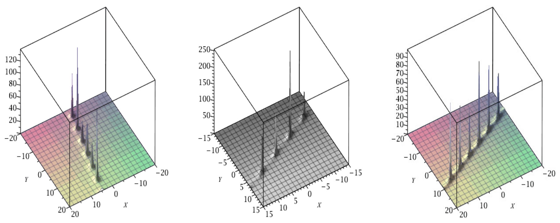
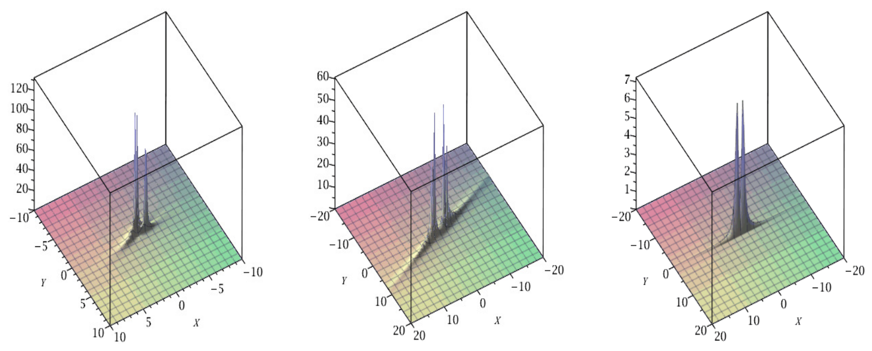
We give some figures in the ( x , y ) plane of coordinates (Figure 21, Figure 22 and Figure 23).
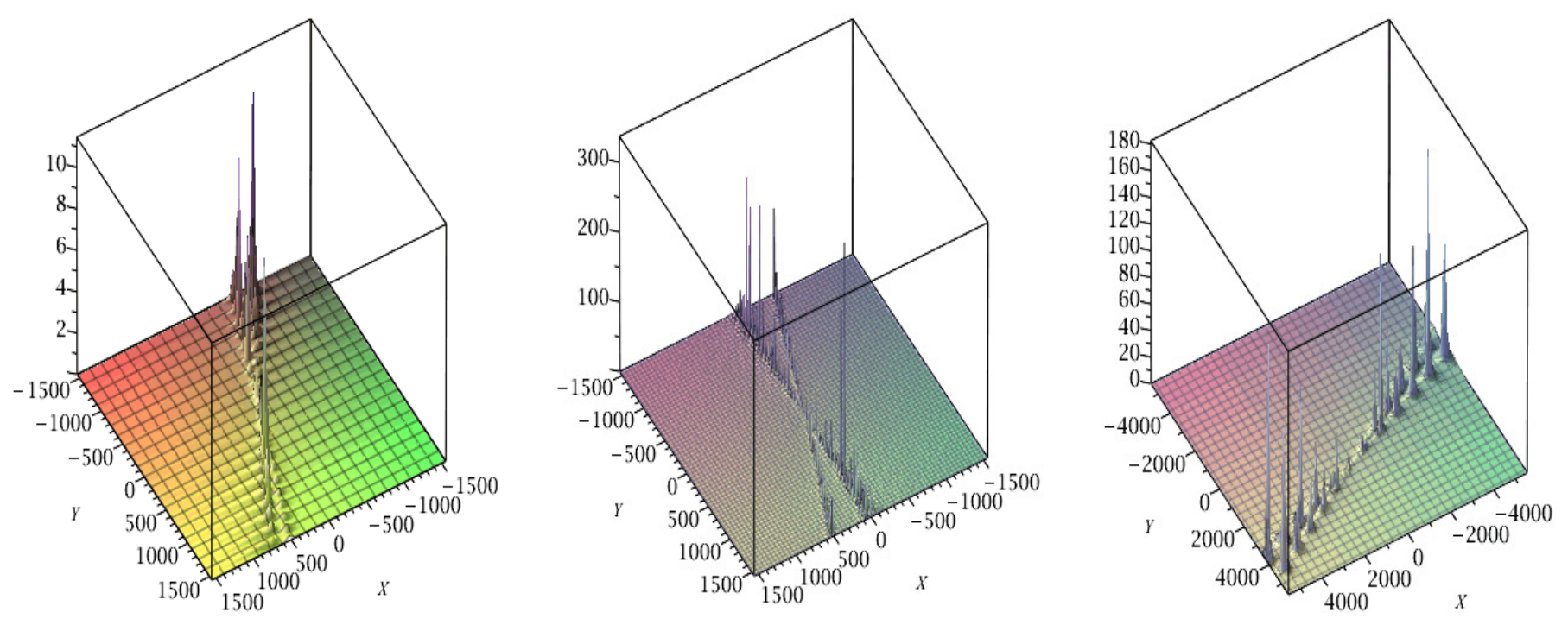
There is a formation of multiple lines of lumps meeting at the same point, which varies according to the values of the parameters. A maximum of three lines is observed.
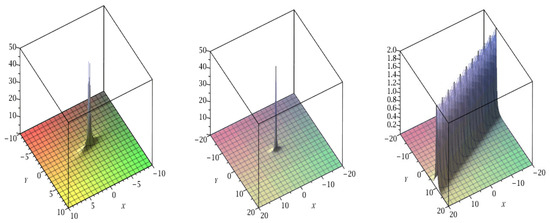
Figure 21. Solutions of order 1 to the KP equation (D = 0, S = 2) for t = 0 , a 1 = 1 , b 1 , 1 , 0 = 1 , b 1 , 2 , 0 = 2 , g 1 , 1 = 0.1 , g 1 , 2 = 2 , h 1 , 1 = 1 , h 1 , 2 = 2 , d 1 , 1 = 1 , d 1 , 2 = 2 , e 1 , 1 = 1 , e 1 , 2 = 2 (left); for t = 0 , a 1 = 1 , b 1 , 1 , 0 = 1 , b 1 , 2 , 0 = 2 , g 1 , 1 = 1 , g 1 , 2 = 0.1 , h 1 , 1 = 1 , h 1 , 2 = 2 , d 1 , 1 = 1 , d 1 , 2 = 2 , e 1 , 1 = 1 , e 1 , 2 = 2 (center); for t = 0 , a 1 = 1 , b 1 , 1 , 0 = 1 , b 1 , 2 , 0 = 2 , g 1 , 1 = 1 , g 1 , 2 = 2 , h 1 , 1 = 0.5 , h 1 , 2 = 2 , d 1 , 1 = 1 , d 1 , 2 = 2 , e 1 , 1 = 1 , e 1 , 2 = 2 (right).
Axioms 15 00586 g021
Figure 22. Solutions of order 1 to the KP equation (D = 0, S = 2) for t = 0 , a 1 = 1 , b 1 , 1 , 0 = 1 , b 1 , 2 , 0 = 2 , g 1 , 1 = 1 , g 1 , 2 = 2 , h 1 , 1 = 1 , h 1 , 2 = 0.5 , d 1 , 1 = 1 , d 1 , 2 = 2 , e 1 , 1 = 1 , e 1 , 2 = 2 (left); for t = 0 , a 1 = 1 , b 1 , 1 , 0 = 1 , b 1 , 2 , 0 = 2 , g 1 , 1 = 1 , g 1 , 2 = 2 , h 1 , 1 = 1 , h 1 , 2 = 2 , d 1 , 1 = 0.1 , d 1 , 2 = 2 , e 1 , 1 = 1 , e 1 , 2 = 2 (center); for t = 0 , a 1 = 1 , b 1 , 1 , 0 = 1 , b 1 , 2 , 0 = 2 , g 1 , 1 = 1 , g 1 , 2 = 2 , h 1 , 1 = 1 , h 1 , 2 = 2 , d 1 , 1 = 1 , d 1 , 2 = 0.5 , e 1 , 1 = 1 , e 1 , 2 = 2 (right).
Axioms 15 00586 g022
Figure 23. Solutions of order 1 to the KP equation (D = 0, S = 2) for t = 0 , a 1 = 1 , b 1 , 1 , 0 = 1 , b 1 , 2 , 0 = 2 , g 1 , 1 = 1 , g 1 , 2 = 2 , h 1 , 1 = 1 , h 1 , 2 = 2 , d 1 , 1 = 1 , d 1 , 2 = 2 , e 1 , 1 = 0.1 , e 1 , 2 = 2 (left); for t = 0 , a 1 = 1 , b 1 , 1 , 0 = 1 , b 1 , 2 , 0 = 2 , g 1 , 1 = 1 , g 1 , 2 = 2 , h 1 , 1 = 1 , h 1 , 2 = 2 , d 1 , 1 = 1 , d 1 , 2 = 2 , e 1 , 1 = 1 , e 1 , 2 = 0.1 (center); for t = 0 , a 1 = 1 , b 1 , 1 , 0 = 1 , b 1 , 2 , 0 = 2 , g 1 , 1 = 1 , g 1 , 2 = 2 , h 1 , 1 = 1 , h 1 , 2 = 2 , d 1 , 1 = 1 , d 1 , 2 = 2 , e 1 , 1 = 1 , e 1 , 2 = 2 (right).
Axioms 15 00586 g023
In order not to overload the text, we will end the study of the case D = 0 here.

3.3. Solutions with One Degree of Summation (S = 1)

In this section, we construct solutions to the Kadomtsev–Petviashvili (KP) equation by using the previous Darboux transformation with particular generating functions, but limited to one degree of summation.
With this choice, we get rational solutions expressed in terms of a Wronskian of order N depending on N ( D + 5 ) real parameters.
  • In this case, we construct explicitly multi-parametric rational solutions to the KP equation, and we study the patterns of their modulus in the ( x , y ) plane and their evolution according to time and parameters.
We will call the order N of the Wronskian the order of the solution. The number of terms in the summation, S, will be called the degree of summation of the solution, and D the degree of derivation of the solution.

3.3.1. Rational Solutions (S = 1)

We consider b j d , d j , e j , g j , and h j to be arbitrary real numbers, with c j = g j + i h j .
We consider the elementary functions f j defined by
f j ( x , y , t ) = e i c j x i c j 2 y + i c j 3 t + d j + i e j = e i ( g j + i h j ) x i ( g j + i h j ) 2 y + i ( g j + i h j ) 3 t + d j + i e j .
Then, we have the following theorem.
Theorem 9. 
Let ϕ j be the functions defined by
ϕ j ( x , y , t ) = d = 0 D b j d c j d e i c j x i c j 2 y + i c j 3 t + d j + i e j = d = 0 D b j d c j d f j ( x , y , t ) .
Then the function u defined by
u ( x , y , t ) = 2 x 2 ln ( W ( ϕ 1 ( x , y , t ) , , ϕ N ( x , y , t ) )
is a rational solution to the KP Equation (1) depending on real N ( D + 5 ) parameters b j , d , g j , h j , d j , and e j , 1 j N , 0 d D .
Proof. 
From the previous result, by choosing S = 1 and a j = 1 , we already know that (73) is a solution to the KP equation.
It remains to be proven that this solution is rational.
  • c j d f j ( x , y , t ) can be written as p j d ( x , y , t ) f j ( x , y , t ) , where p j d ( x , y , t ) is a polynomial in x, y and t, so
ϕ j ( x , y , t ) = d = 0 D b j d p j d ( x , y , t ) f j ( x , y , t ) = f j ( x , y , t ) d = 0 D b j d p j d ( x , y , t ) = P j ( x , y , t ) f j ( x , y , t ) ,
where P j ( x , y , t ) is a polynomial in x, y and t.
The derivation with respect to x of ϕ j ( x , y , t ) , then, is equal to x k ϕ j ( x , y , t ) = Q j , k ( x , y , t ) f j ( x , y , t ) , where Q j , k ( x , y , t ) is a polynomial in x, y and t. We denote by Q j , 0 ( x , y , t ) the polynomial P j ( x , y , t ) .
The Wronskian W ( ϕ 1 , , ϕ N ) can be written as
Q 1 , 0 ( x , y , t ) f 1 ( x , y , t ) Q 2 , 0 ( x , y , t ) f 2 ( x , y , t ) Q N , 0 ( x , y , t ) f N ( x , y , t ) Q 1 , 1 ( x , y , t ) f 1 ( x , y , t ) Q 2 , 1 ( x , y , t ) f 2 ( x , y , t ) Q N , 1 ( x , y , t ) f N ( x , y , t ) Q 1 , N 1 ( x , y , t ) f 1 ( x , y , t ) Q 2 , N 1 ( x , y , t ) f 2 ( x , y , t ) Q N , N 1 ( x , y , t ) f N ( x , y , t )
It can be rewritten as
W ( ϕ 1 , , ϕ N ) = k = 1 N f k ( x , y , t )
× Q 1 , 0 ( x , y , t ) Q 2 , 0 ( x , y , t ) Q N , 0 ( x , y , t ) Q 1 , 1 ( x , y , t ) Q 2 , 1 ( x , y , t ) Q N , 1 ( x , y , t ) Q 1 , N 1 ( x , y , t ) Q 2 , N 1 ( x , y , t ) Q N , N 1 ( x , y , t )
or as the product
W ( ϕ 1 , , ϕ N ) = k = 1 N f k ( x , y , t ) × Δ
where Δ is a polynomial in x, y and t.
ln k = 1 N f k ( x , y , t ) = k = 1 N ln f k ( x , y , t ) = k = 1 N i c k x i c k 2 y + i c k 3 t + d k + i e k
so
x 2 ln k = 1 N f k ( x , y , t ) = 0
So we have
u ( x , y , t ) = 2 x 2 ln W ( ϕ 1 ( x , y , t ) , , ϕ N ( x , y , t ) ) = 2 x 2 ln Δ = Δ 2 x Δ Δ x 2 Δ 2
as a rational solution to the KP equation, which proves the result. □

3.3.2. Case D = 1 with Six Real Parameters (S = 1)

The case D = 0 is not interesting because we get the solution u = 0 .
In the case D = 1 , solutions to the KP equation can be written as
u ( x , y , t ) = 2 b 1 , 1 2 ( i b 1 , 1 x + b 1 , 0 + 3 i t b 1 , 1 g 1 2 3 i t b 1 , 1 h 1 2 2 i y b 1 , 1 g 1 + 2 y b 1 , 1 h 1 6 t b 1 , 1 g 1 h 1 ) 2 .
In this case, we observe lumps whose intensities depend on six real parameters. If b 1 , 1 = 0 , we get the solution u = 0 .
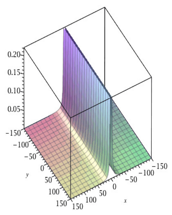
We give some figures in the ( x , y ) plane of coordinates (Figure 24 and Figure 25).
In the two previous figures, we obtain lumps whose moduli depend on the values of the parameters, and we remark that these structures are more sensitive to g 1 and h 1 parameters than to others.

3.3.3. Case D = 2 with Seven Real Parameters (S = 1)

In this case, we take D = 2 ; the solutions to the KP equation can be written as
u ( x , y , t ) = 2 n ( x , y , t ) d ( x , y , t ) 2
with
n ( x , y , t ) = 2 b 1 , 2 2 x 2 + ( 12 t b 1 , 2 2 h 1 2 + 8 y b 1 , 2 2 g 1 12 t b 1 , 2 2 g 1 2 + 8 i y b 1 , 2 2 h 1 24 i t b 1 , 2 2 g 1 h 1 + 2 i b 1 , 1 b 1 , 2 ) x + 72 i t 2 b 1 , 2 2 g 1 h 1 3 12 i t b 1 , 2 2 g 1 6 i t b 1 , 1 b 1 , 2 h 1 2 2 b 1 , 0 b 1 , 2 + 108 t 2 b 1 , 2 2 g 1 2 h 1 2 + 24 t y b 1 , 2 2 g 1 3 + 6 i t b 1 , 1 b 1 , 2 g 1 2 + 4 y b 1 , 1 b 1 , 2 h 1 16 i y 2 b 1 , 2 2 g 1 h 1 12 t b 1 , 1 b 1 , 2 g 1 h 1 18 t 2 b 1 , 2 2 g 1 4 + 12 t b 1 , 2 2 h 1 + b 1 , 1 2 + 8 y 2 b 1 , 2 2 h 1 2 24 i t y b 1 , 2 2 h 1 3 + 4 i y b 1 , 2 2 72 i t 2 b 1 , 2 2 g 1 3 h 1 72 t y b 1 , 2 2 g 1 h 1 2 4 i y b 1 , 1 b 1 , 2 g 1 18 t 2 b 1 , 2 2 h 1 4 + 72 i t y b 1 , 2 2 g 1 2 h 1 8 y 2 b 1 , 2 2 g 1 2 .
And
d ( x , y , t ) = b 1 , 2 x 2 + ( 6 t b 1 , 2 g 1 2 + 12 i t b 1 , 2 g 1 h 1 6 t b 1 , 2 h 1 2 4 y b 1 , 2 g 1 4 i b 1 , 2 y h 1 i b 1 , 1 ) x + 9 t 2 b 1 , 2 g 1 4 + 12 i t y b 1 , 2 h 1 3 54 t 2 b 1 , 2 g 1 2 h 1 2 36 i b 1 , 2 t g 1 2 y h 1 + 9 t 2 b 1 , 2 h 1 4 12 t y b 1 , 2 g 1 3 6 i b 1 , 2 t g 1 + 36 t y b 1 , 2 g 1 h 1 2 + 2 i y b 1 , 1 g 1 + 4 y 2 b 1 , 2 g 1 2 + 36 i t 2 b 1 , 2 g 1 3 h 1 4 y 2 b 1 , 2 h 1 2 + 2 i y b 1 , 2 + 6 t b 1 , 1 g 1 h 1 36 i b 1 , 2 t 2 g 1 h 1 3 + 8 i y 2 b 1 , 2 g 1 h 1 + 6 t b 1 , 2 h 1 + 3 i t b 1 , 1 h 1 2 2 y b 1 , 1 h 1 3 i b 1 , 1 t g 1 2 b 1 , 0 .
We give some figures in the ( x , y ) plane of coordinates. (Figure 26 and Figure 27)
In the two previous figures, we get lumps whose moduli depend on the values of parameters. These structures are more sensitive to g 1 and h 1 parameters than to others. In this case, we observe a maximum of two isolated lumps, as shown, for example, in Figure 4, center.

3.3.4. Case D = 3 with Eight Real Parameters (S = 1)

In the case D = 3 , we observe multiple lumps. As in the previous cases, these structures are more sensitive to g 1 and h 1 parameters than to others.
The solutions to the KP equation can be written as
u ( x , y , t ) = 2 n ( x , y , t ) d ( x , y , t ) 2
with
n ( x , y , t ) = 3 b 1 , 3 2 x 4 + ( 36 t b 1 , 3 2 h 1 2 + 36 t b 1 , 3 2 g 1 2 24 y b 1 , 3 2 g 1 + 72 i t b 1 , 3 2 g 1 h 1 24 i y b 1 , 3 2 h 1 4 i b 1 , 2 b 1 , 3 ) x 3 + ( 216 i t y b 1 , 3 2 h 1 3 + 162 t 2 b 1 , 3 2 g 1 4 36 i t b 1 , 2 b 1 , 3 g 1 2 648 i t 2 b 1 , 3 2 g 1 h 1 3 972 t 2 b 1 , 3 2 g 1 2 h 1 2 + 162 t 2 b 1 , 3 2 h 1 4 2 b 1 , 2 2 + 648 i t 2 b 1 , 3 2 g 1 3 h 1 + 648 t y b 1 , 3 2 g 1 h 1 2 + 36 i t b 1 , 2 b 1 , 3 h 1 2 24 y b 1 , 2 b 1 , 3 h 1 648 i t y b 1 , 3 2 g 1 2 h 1 + 144 i y 2 b 1 , 3 2 g 1 h 1 216 t y b 1 , 3 2 g 1 3 + 72 t b 1 , 2 b 1 , 3 g 1 h 1 72 y 2 b 1 , 3 2 h 1 2 + 72 y 2 b 1 , 3 2 g 1 2 + 24 i y b 1 , 2 b 1 , 3 g 1 ) x 2 + ( 1728 i t y 2 b 1 , 3 2 g 1 3 h 1 1728 i t y 2 b 1 , 3 2 g 1 h 1 3 + 648 i t 2 b 1 , 2 b 1 , 3 g 1 2 h 1 2 + 144 i t y b 1 , 2 b 1 , 3 g 1 3 3240 i t 2 y b 1 , 3 2 g 1 4 h 1 + 6480 i t 2 y b 1 , 3 2 g 1 2 h 1 3 432 t y b 1 , 2 b 1 , 3 g 1 2 h 1 4860 t 3 b 1 , 3 2 g 1 4 h 1 2 + 4860 t 3 b 1 , 3 2 g 1 2 h 1 4 + 432 t y 2 b 1 , 3 2 h 1 4 + 96 i y 3 b 1 , 3 2 h 1 3 + 8 i y b 1 , 2 2 h 1 + 432 t y 2 b 1 , 3 2 g 1 4 648 t 2 y b 1 , 3 2 g 1 5 + 288 y 3 b 1 , 3 2 g 1 h 1 2 432 i t y b 1 , 2 b 1 , 3 g 1 h 1 2 + 36 t b 1 , 3 2 48 i y 2 b 1 , 2 b 1 , 3 g 1 2 + 48 i y 2 b 1 , 2 b 1 , 3 h 1 2 24 i t b 1 , 2 2 g 1 h 1 108 i t 2 b 1 , 2 b 1 , 3 g 1 4 108 i t 2 b 1 , 2 b 1 , 3 h 1 4 288 i y 3 b 1 , 3 2 g 1 2 h 1 648 i t 2 y b 1 , 3 2 h 1 5 + 1944 i t 3 b 1 , 3 2 g 1 5 h 1 6480 i t 3 b 1 , 3 2 g 1 3 h 1 3 + 1944 i t 3 b 1 , 3 2 g 1 h 1 5 + 96 y 2 b 1 , 2 b 1 , 3 g 1 h 1 + 432 t 2 b 1 , 2 b 1 , 3 g 1 3 h 1 432 t 2 b 1 , 2 b 1 , 3 g 1 h 1 3 + 144 t y b 1 , 2 b 1 , 3 h 1 3 2592 t y 2 b 1 , 3 2 g 1 2 h 1 2 + 6480 t 2 y b 1 , 3 2 g 1 3 h 1 2 3240 t 2 y b 1 , 3 2 g 1 h 1 4 12 t b 1 , 2 2 g 1 2 + 12 t b 1 , 2 2 h 1 2 + 8 y b 1 , 2 2 g 1 6 i b 1 , 0 b 1 , 3 + 2 i b 1 , 1 b 1 , 2 + 324 t 3 b 1 , 3 2 g 1 6 324 t 3 b 1 , 3 2 h 1 6 96 y 3 b 1 , 3 2 g 1 3 ) x + 13608 t 3 y b 1 , 3 2 g 1 5 h 1 2 22680 t 3 y b 1 , 3 2 g 1 3 h 1 4 2160 t 3 b 1 , 2 b 1 , 3 g 1 3 h 1 3 + 648 t 3 b 1 , 2 b 1 , 3 g 1 h 1 5 + 2880 t y 3 b 1 , 3 2 g 1 3 h 1 2 1440 t y 3 b 1 , 3 2 g 1 h 1 4 216 t 2 y b 1 , 2 b 1 , 3 h 1 5 96 i y 3 b 1 , 2 b 1 , 3 g 1 h 1 2 + 72 i t y b 1 , 2 2 g 1 2 h 1 144 i t y 2 b 1 , 2 b 1 , 3 g 1 4 144 i t y 2 b 1 , 2 b 1 , 3 h 1 4 + 4536 t 3 y b 1 , 3 2 g 1 h 1 6 + 1620 i t 3 b 1 , 2 b 1 , 3 g 1 4 h 1 2 1620 i t 3 b 1 , 2 b 1 , 3 g 1 2 h 1 4 1440 i t y 3 b 1 , 3 2 g 1 4 h 1 + 2880 i t y 3 b 1 , 3 2 g 1 2 h 1 3 + 3888 i t 2 y 2 b 1 , 3 2 g 1 5 h 1 12960 i t 2 y 2 b 1 , 3 2 g 1 3 h 1 3 + 3888 i t 2 y 2 b 1 , 3 2 g 1 h 1 5 4536 i t 3 y b 1 , 3 2 g 1 6 h 1 + 22680 i t 3 y b 1 , 3 2 g 1 4 h 1 3 13608 i t 3 y b 1 , 3 2 g 1 2 h 1 5 + 1080 i t 2 y b 1 , 2 b 1 , 3 g 1 h 1 4 + 864 i t y 2 b 1 , 2 b 1 , 3 g 1 2 h 1 2 + 216 i t 2 y b 1 , 2 b 1 , 3 g 1 5 + 1944 i t 4 b 1 , 3 2 g 1 7 h 1 13608 i t 4 b 1 , 3 2 g 1 5 h 1 3 + 13608 i t 4 b 1 , 3 2 g 1 3 h 1 5 1944 i t 4 b 1 , 3 2 g 1 h 1 7 + 648 i t 3 y b 1 , 3 2 h 1 7 108 i t 3 b 1 , 2 b 1 , 3 g 1 6 + 108 i t 3 b 1 , 2 b 1 , 3 h 1 6 288 i t y 3 b 1 , 3 2 h 1 5 + 192 i y 4 b 1 , 3 2 g 1 3 h 1 192 i y 4 b 1 , 3 2 g 1 h 1 3 72 i t 2 b 1 , 2 2 g 1 3 h 1 + 72 i t 2 b 1 , 2 2 g 1 h 1 3 + 32 i y 3 b 1 , 2 b 1 , 3 g 1 3 + 36 i t b 1 , 1 b 1 , 3 g 1 9720 t 2 y 2 b 1 , 3 2 g 1 4 h 1 2 + 9720 t 2 y 2 b 1 , 3 2 g 1 2 h 1 4 + 648 t 3 b 1 , 2 b 1 , 3 g 1 5 h 1 432 i t 2 b 1 , 3 2 g 1 h 1 16 i y 2 b 1 , 2 2 g 1 h 1 + 144 i t y b 1 , 3 2 h 1 18 i t b 1 , 0 b 1 , 3 g 1 2 + 18 i t b 1 , 0 b 1 , 3 h 1 2 + 6 i t b 1 , 1 b 1 , 2 g 1 2 6 i t b 1 , 1 b 1 , 2 h 1 2 648 t 2 y 2 b 1 , 3 2 h 1 6 288 y 4 b 1 , 3 2 g 1 2 h 1 2 + 108 t 2 b 1 , 2 2 g 1 2 h 1 2 + 32 y 3 b 1 , 2 b 1 , 3 h 1 3 + 24 t y b 1 , 2 2 g 1 3 12 y b 1 , 0 b 1 , 3 h 1 + 4 y b 1 , 1 b 1 , 2 h 1 6804 t 4 b 1 , 3 2 g 1 6 h 1 2 + 17010 t 4 b 1 , 3 2 g 1 4 h 1 4 6804 t 4 b 1 , 3 2 g 1 2 h 1 6 + b 1 , 1 2 + 36 t b 1 , 0 b 1 , 3 g 1 h 1 12 t b 1 , 1 b 1 , 2 g 1 h 1 96 y 3 b 1 , 2 b 1 , 3 g 1 2 h 1 72 t y b 1 , 2 2 g 1 h 1 2 2160 i t 2 y b 1 , 2 b 1 , 3 g 1 3 h 1 2 2 b 1 , 0 b 1 , 2 36 y 2 b 1 , 3 2 12 i t b 1 , 2 2 g 1 12 i t b 1 , 2 b 1 , 3 12 i y b 1 , 1 b 1 , 3 36 t b 1 , 1 b 1 , 3 h 1 + 144 t y b 1 , 3 2 g 1 648 t 3 y b 1 , 3 2 g 1 7 + 648 t 2 y 2 b 1 , 3 2 g 1 6 288 t y 3 b 1 , 3 2 g 1 5 + 576 t y 2 b 1 , 2 b 1 , 3 g 1 3 h 1 576 t y 2 b 1 , 2 b 1 , 3 g 1 h 1 3 1080 t 2 y b 1 , 2 b 1 , 3 g 1 4 h 1 + 2160 t 2 y b 1 , 2 b 1 , 3 g 1 2 h 1 3 + 12 i y b 1 , 0 b 1 , 3 g 1 4 i y b 1 , 1 b 1 , 2 g 1 24 i t y b 1 , 2 2 h 1 3 + 4 i y b 1 , 2 2 + 216 t 2 b 1 , 3 2 h 1 2 + 243 t 4 b 1 , 3 2 g 1 8 + 243 t 4 b 1 , 3 2 h 1 8 + 48 y 4 b 1 , 3 2 h 1 4 18 t 2 b 1 , 2 2 g 1 4 18 t 2 b 1 , 2 2 h 1 4 8 y 2 b 1 , 2 2 g 1 2 + 8 y 2 b 1 , 2 2 h 1 2 + 12 t b 1 , 2 2 h 1 216 t 2 b 1 , 3 2 g 1 2 + 48 y 4 b 1 , 3 2 g 1 4 .
d ( x , y , t ) = i b 1 , 3 x 3 + ( 9 i t b 1 , 3 g 1 2 18 t b 1 , 3 g 1 h 1 9 i t b 1 , 3 h 1 2 6 i y b 1 , 3 g 1 + 6 y b 1 , 3 h 1 + b 1 , 2 ) x 2 + ( 27 i t 2 b 1 , 3 g 1 4 108 t 2 b 1 , 3 g 1 3 h 1 162 i t 2 b 1 , 3 g 1 2 h 1 2 + 108 t 2 b 1 , 3 g 1 h 1 3 + 27 i t 2 b 1 , 3 h 1 4 36 i t y b 1 , 3 g 1 3 + 108 t y b 1 , 3 g 1 2 h 1 + 108 i t y b 1 , 3 g 1 h 1 2 36 t y b 1 , 3 h 1 3 + 12 i y 2 b 1 , 3 g 1 2 24 y 2 b 1 , 3 g 1 h 1 12 i y 2 b 1 , 3 h 1 2 + 6 t b 1 , 2 g 1 2 + 12 i t b 1 , 2 g 1 h 1 6 t b 1 , 2 h 1 2 + 18 t b 1 , 3 g 1 + 18 i t b 1 , 3 h 1 4 y b 1 , 2 g 1 4 i y b 1 , 2 h 1 6 y b 1 , 3 i b 1 , 1 ) x 54 t 2 b 1 , 2 g 1 2 h 1 2 b 1 , 0 162 t 3 b 1 , 3 g 1 h 1 5 + 54 t 2 y b 1 , 3 h 1 5 4 y 2 b 1 , 2 h 1 2 162 t 3 b 1 , 3 g 1 5 h 1 + 9 t 2 b 1 , 2 h 1 4 + 4 y 2 b 1 , 2 g 1 2 8 y 3 b 1 , 3 h 1 3 2 y b 1 , 1 h 1 + 9 t 2 b 1 , 2 g 1 4 + 54 t 2 b 1 , 3 g 1 3 + 12 y 2 b 1 , 3 g 1 54 i t 2 b 1 , 3 h 1 3 + 12 i y 2 b 1 , 3 h 1 + 27 i t 3 b 1 , 3 g 1 6 27 i t 3 b 1 , 3 h 1 6 8 i y 3 b 1 , 3 g 1 3 + 3 i t b 1 , 1 h 1 2 6 i t b 1 , 2 g 1 3 i t b 1 , 1 g 1 2 + 2 i y b 1 , 1 g 1 + 6 t b 1 , 2 h 1 + 2 i y b 1 , 2 6 i t b 1 , 3 + 36 i t 2 b 1 , 2 g 1 3 h 1 36 i t 2 b 1 , 2 g 1 h 1 3 + 12 i t y b 1 , 2 h 1 3 + 8 i y 2 b 1 , 2 g 1 h 1 405 i t 3 b 1 , 3 g 1 4 h 1 2 54 i t 2 y b 1 , 3 g 1 5 + 405 i t 3 b 1 , 3 g 1 2 h 1 4 + 36 i t y 2 b 1 , 3 g 1 4 + 36 i t y 2 b 1 , 3 h 1 4 + 24 i y 3 b 1 , 3 g 1 h 1 2 + 162 i t 2 b 1 , 3 g 1 2 h 1 + 24 y 3 b 1 , 3 g 1 2 h 1 162 t 2 b 1 , 3 g 1 h 1 2 + 54 t y b 1 , 3 h 1 2 + 6 t b 1 , 1 g 1 h 1 12 t y b 1 , 2 g 1 3 + 540 t 3 b 1 , 3 g 1 3 h 1 3 54 t y b 1 , 3 g 1 2 108 i t y b 1 , 3 g 1 h 1 270 i t 2 y b 1 , 3 g 1 h 1 4 216 i t y 2 b 1 , 3 g 1 2 h 1 2 + 540 i t 2 y b 1 , 3 g 1 3 h 1 2 36 i t y b 1 , 2 g 1 2 h 1 + 36 t y b 1 , 2 g 1 h 1 2 144 t y 2 b 1 , 3 g 1 3 h 1 + 270 t 2 y b 1 , 3 g 1 4 h 1 + 144 t y 2 b 1 , 3 g 1 h 1 3 540 t 2 y b 1 , 3 g 1 2 h 1 3 .
We give some figures in the ( x , y ) plane of coordinates (Figure 28 and Figure 29).

3.4. Other Types of Choices of S, D, N

We present different cases of solutions depending on the values of N, S and D.

3.4.1. Case S = 2 , D = 1

In this case, solutions to the KP equation can be written as
v ( x , y , t ) = 2 n ( x , y , t ) d ( x , y , t ) 2
with
n ( x , y , t ) = 2 i e i x i y + i t x + 4 i e i x i y + i t y 6 i e i x i y + i t t + 4 e 2 i x 2 i y + 2 i t 6 e i x i y + i t .
  • and
d ( x , y , t ) = 2 i e i ( x + t y ) x + 1 + 2 e i ( x + t y ) 4 i y e i ( x + t y ) + 6 i t e i ( x + t y ) .
We give some figures in the ( x , y ) plane of coordinates (Figure 30).

3.4.2. Case S = 2 , D = 2

In this case, solutions to the KP equation can be written as
v ( x , y , t ) = 2 n ( x , y , t ) d ( x , y , t ) 2
with
n ( x , y , t ) = ( 2 e i x i y + i t 8 e 2 i x 2 i y + 2 i t ) x 2 + ( 10 i e i x i y + i t + 12 e i x i y + i t t + 32 e 2 i x 2 i y + 2 i t y 48 e 2 i x 2 i y + 2 i t t + 8 i e 2 i x 2 i y + 2 i t 8 e i x i y + i t y ) x 24 e i x i y + i t y t + 8 e i x i y + i t y 2 + 18 e i x i y + i t t 2 32 e 2 i x 2 i y + 2 i t y 2 72 e 2 i x 2 i y + 2 i t t 2 24 i e 2 i x 2 i y + 2 i t t 10 e i x i y + i t 4 e 2 i x 2 i y + 2 i t + 24 i e i x i y + i t y + 96 e 2 i x 2 i y + 2 i t y t 42 i e i x i y + i t t .
And
d ( x , y , t ) = 2 e i ( x + t y ) x 2 + ( 2 i e i ( x + t y ) + 8 y e i ( x + t y ) 12 t e i ( x + t y ) ) x + 1 + 2 e i ( x + t y ) 8 i y e i ( x + t y ) 8 y 2 e i ( x + t y ) 18 t 2 e i ( x + t y ) + 18 i t e i ( x + t y ) + 24 t y e i ( x + t y ) .
We give some figures in the ( x , y ) plane of coordinates (Figure 31).

3.4.3. Case S = 2 , D = 3

In this case, solutions to the KP equation can be written as
v ( x , y , t ) = 2 n ( x , y , t ) d ( x , y , t ) 2
with
n ( x , y , t ) = 12 e 2 i x 2 i y + 2 i t x 4 + ( 96 e 2 i x 2 i y + 2 i t y 16 i e 2 i x 2 i y + 2 i t + 2 i e i x i y + i t + 144 e 2 i x 2 i y + 2 i t t ) ) x 3 + ( 96 i e 2 i x 2 i y + 2 i t y 8 e 2 i x 2 i y + 2 i t 864 e 2 i x 2 i y + 2 i t t y 12 i e i x i y + i t y + 18 i e i x i y + i t t + 14 e i x i y + i t 144 i e 2 i x 2 i y + 2 i t t + 648 e 2 i x 2 i y + 2 i t t 2 + 288 e 2 i x 2 i y + 2 i t y 2 ) ) x 2 + ( 432 i e 2 i x 2 i y + 2 i t t 2 22 i e i x i y + i t + 1296 e 2 i x 2 i y + 2 i t t 3 2592 e 2 i x 2 i y + 2 i t t 2 y + 576 i e 2 i x 2 i y + 2 i t t y + 54 i e i x i y + i t t 2 + 120 e i x i y + i t t 68 e i x i y + i t y + 96 e 2 i x 2 i y + 2 i t t + 32 e 2 i x 2 i y + 2 i t y 384 e 2 i x 2 i y + 2 i t y 3 + 24 i e i x i y + i t y 2 + 1728 e 2 i x 2 i y + 2 i t t y 2 16 i e 2 i x 2 i y + 2 i t 192 i e 2 i x 2 i y + 2 i t y 2 72 i e i x i y + i t t y ) ) x 10 e i x i y + i t 4 e 2 i x 2 i y + 2 i t 16 i e i x i y + i t y 3 + 54 i e i x i y + i t t 3 + 2592 e 2 i x 2 i y + 2 i t t 2 y 2 1152 e 2 i x 2 i y + 2 i t t y 3 276 e i x i y + i t y t + 672 e 2 i x 2 i y + 2 i t t y 162 i e i x i y + i t t + 72 i e i x i y + i t y 432 i e 2 i x 2 i y + 2 i t t 3 + 128 i e 2 i x 2 i y + 2 i t y 3 + 192 e 2 i x 2 i y + 2 i t y 4 936 e 2 i x 2 i y + 2 i t t 2 + 80 e i x i y + i t y 2 + 234 e i x i y + i t t 2 176 e 2 i x 2 i y + 2 i t y 2 2592 e 2 i x 2 i y + 2 i t t 3 y + 972 e 2 i x 2 i y + 2 i t t 4 + 72 i e i x i y + i t y 2 t 108 i e i x i y + i t t 2 y 576 i e 2 i x 2 i y + 2 i t t y 2 + 864 i e 2 i x 2 i y + 2 i t t 2 y .
d ( x , y , t ) = 2 i e i ( x + t y ) ) x 3 + ( 2 e i ( x + t y ) ) + 18 i t e i ( x + t y ) ) 12 i y e i ( x + t y ) ) ) ) x 2 + ( 54 i e i ( x + t y ) ) t 2 + 24 i y 2 e i ( x + t y ) ) + 48 t e i ( x + t y ) ) 20 y e i ( x + t y ) ) 2 i e i ( x + t y ) ) 72 i e i ( x + t y ) ) y t ) ) x 1 2 e i ( x + t y ) ) 108 i t 2 y e i ( x + t y ) ) + 54 i t 3 e i ( x + t y ) ) + 72 i t y 2 e i ( x + t y ) ) + 8 i y e i ( x + t y ) ) 16 i y 3 e i ( x + t y ) ) 132 t y e i ( x + t y ) ) 30 i t e i ( x + t y ) ) + 32 y 2 e i ( x + t y ) ) + 126 t 2 e i ( x + t y ) ) .
We give some figures in the ( x , y ) plane of coordinates (Figure 32).

4. From Particular Polynomials

In this section we always consider the Kadomtsev–Petviashvili (KP) equation defined by (1).
We construct solutions to the KP equation from particular polynomials. We obtain rational solutions written as second derivatives with respect to the variable x of the logarithm of a determinant of order n. So, with this method, we get an infinite hierarchy of rational solutions to the KP equation.
We give the explicit expressions of these solutions for the first five orders.

4.1. Rational Solutions to the KP Equation

We consider the particular polynomials p n defined by
p n ( x , y , t ) = k 1 = 0 n x k 1 k 2 = 0 n k 1 y k 2 2 1 1 2 k 2 2 k 2 2 k 2 2 ! × t n k 1 k 2 3 n k 1 k 2 3 ! × 1 1 2 n k 1 k 2 + 1 3 n k 1 k 2 3 ,   for   n 0 , p n ( x , y , t ) = 0 ,   for   n < 0 .
In the previous definition of p n , [ x ] means the greater integer less than or equal to x. We consider the following determinant:
det ( p n i + j ( x , t ) ) { 1 i n , 1 j n } ,
or, in other words, it can be written as
p n p n + 1 p n + 2 p 2 n 1 p n 1 p n p n + 1 p 2 n 2 p 1 p 2 p 3 p n .
With these polynomials, we construct a type of rational solution to the KP equation. We prove this result by using the Hirota method. This method gives some rational solutions to the KP equation.
With these notations and x 2 = 2 x 2 , we have the following result.
Theorem 10. 
The function v n ( x , y , t ) defined by
v n ( x , y , t ) = 2 x 2 ( det ( p n i + j ( x , t ) ) { 1 i n , 1 j n } )
is a rational solution to the KP Equation (1):
( 4 u t 6 u u x + u x x x ) x 3 u y y = 0 .
Proof. 
From the bilinear method, v n ( x , y , t ) = 2 x 2 ( ln f ( x , y , t ) ) is a solution to the KP equation if f satisfies the following equation:
( D x 4 4 D x D t + 3 D y 2 ) f · f = 0 ,
where D is the bilinear differential operator.
We have to verify (78) for f = det ( p n i + j ( x , t ) ) { 1 i n , 1 j n } . We denote by C j the following column vector, for j negative or positive integers:
C j = p n 1 + j p n 2 + j p j .
Then det ( p n i + j ( x , t ) ) { 1 i n , 1 j n } can be written as | C 1 , , C n | .
Let H be the expression H = ( D x 4 4 D x D t + 3 D y 2 ) f · f . We have to evaluate H.
The polynomials p k verify x ( p k ) = p k 1 , y ( p k ) = p k 2 and t ( p k ) = p k 3 .
So H can be written as
H = [ | C 3 , C 2 , C 3 , , C n | + 3 | C 2 , C 1 , C 3 , C 4 , , C n | + 2 | C 1 , C 0 , C 3 , C 4 , , C n | + 3 | C 1 , C 1 , C 2 , C 4 , , C n |   +   | C 0 , C 1 , C 2 , C 3 , C 5 , , C n | ]   ×   | C 1 , C 2 , C 3 , , C n | 4 [ | C 2 , C 2 , C 3 , , C n | + 2 | C 1 , C 1 , C 3 , C 4 , , C n | + | C 0 , C 1 , C 2 , C 4 , C 5 , , C n | ]   ×   | C 0 , C 2 , C 3 , C 4 , , C n | + 3 [ | C 1 , C 2 , C 3 , , C n |   +   | C 0 , C 1 , C 3 , , C n | ] 2 4 [ | C 3 , C 2 , C 3 , , C n | + | C 2 , C 1 , C 3 , C 4 , , C n | + | C 0 , C 1 , C 3 , C 4 , , C n |   +   | C 1 , C 2 , C 3 , C 4 , , C n | + | C 1 , C 1 , C 2 , C 4 , C 5 , , C n |   +   | C 1 , C 2 , C 1 , C 4 , C 5 , , C n | + | C 1 , C 2 , C 0 , C 3 , C 5 , , C n | ]   ×   | C 1 , C 2 , C 3 , , C n | + 4 [ | C 2 , C 2 , C 3 , , C n | + | C 1 , C 1 , C 3 , C 4 , , C n | + | C 1 , C 2 , C 0 , C 4 , C 5 , , C n | ]   ×   | C 0 , C 2 , C 3 , , C n | + 3 [ | C 3 , C 2 , C 3 , , C n | + 2 | C 1 , C 0 , C 3 , C 4 , , C n | + | C 1 , C 2 , C 1 , C 4 , C 5 , , C n | + | C 1 , C 2 , C 3 , C 4 , , C n |   +   | C 1 , C 0 , C 3 , C 2 , C 5 , , C n | ]   ×   | C 1 , C 2 , , C n | 3 [ | C 1 , C 2 , C 3 , , C n |   +   | C 1 , C 0 , C 3 , C 4 , , C n | ] 2
H can be reduced to
H = 3 | C 3 , C 2 , C 3 , , C n |   ×   | C 1 , C 2 , , C n | + 3 | C 2 , C 1 , C 3 , C 4 , , C n |   ×   | C 1 , C 2 , C 3 , , C n | + 6 | C 1 , C 0 , C 3 , C 4 , , C n |   ×   | C 1 , C 2 , , C n | + 3 | C 1 , C 1 , C 2 , C 4 , C 5 , , C n |   ×   | C 1 , C 2 , , C n | 3 | C 0 , C 1 , C 2 , C 3 , C 5 , , C n | ]   ×   | C 1 , C 2 , , C n | 12 [ | C 1 , C 1 , C 3 , C 4 , , C n |   ×   | C 0 , C 2 , C 3 , , C n | + 3 | C 1 , C 2 , C 3 , , C n | 2 + 3 | C 0 , C 1 , C 3 , C 4 , , C n | 2 + 6 | C 1 , C 2 , C 3 , , C n |   ×   | C 0 , C 1 , C 3 , C 4 , , C n | + 3 | C 3 , C 2 , C 3 , , C n |   ×   | C 1 , C 2 , , C n | + 6 | C 1 , C 0 , C 3 , C 4 , , C n |   ×   | C 1 , C 2 , , C n | + 3 | C 1 , C 2 , C 1 , C 4 , C 5 , , C n |   ×   | C 1 , C 2 , , C n | + 3 | C 1 , C 2 , C 3 , C 4 , , C n |   ×   | C 1 , C 2 , , C n | + 3 | C 1 , C 0 , C 3 , C 2 , C 5 , , C n | ]   ×   | C 1 , C 2 , , C n | 3 | C 1 , C 2 , C 3 , , C n | 2 3 | C 1 , C 0 , C 3 , C 4 , , C n | 2 6 | C 1 , C 2 , C 3 , , C n | 2   ×   | C 1 , C 0 , C 3 , C 4 , , C n |
It can be reduced to the following sum of three terms:
H = 12 [ | C 1 , C 0 , C 3 , C 4 , , C n |   ×   | C 1 , C 2 , , C n | | C 1 , C 1 , C 3 , C 4 , , C n |   ×   | C 0 , C 2 , C 3 , , C n | + | C 1 , C 2 , C 3 , , C n |   ×   | C 0 , C 1 , C 3 , C 4 , , C n | ] = 12 H ˜
The last expression H ˜ can be rewritten as the following determinant of order 2 n :
H ˜ = C 1 C 0 C 3 C 4 C n C 1 C 2 0 0 0 C 0 0 0 0 C 1 C 2 C 3 C 4 C 5 C n
It can be rewritten in terms of polynomials p n :
H ˜ = p n 2 p n 1 p n + 2 p n + 3 p 2 n 1 p n p n + 1 0 0 p n 3 p n 2 p n + 1 p n + 1 p 2 n 2 p n 2 p n 0 0 p 1 p 0 p 3 p 4 p n p 1 p 2 0 0 0 p n 1 0 0 0 p n p n + 1 p 2 n 1 0 p n 2 0 0 0 p n 1 p n p 2 n 2 0 p 0 0 0 0 p 1 p 2 p n
We denote by L the rows and by C the columns of this determinant of order 2 n .
We combine the rows of the previous determinant in the following way.
We replace L n + j by L n + j L j + 1 for 1 j n , and then we obtain the following determinant:
H ˜ = p n 2 p n 1 p n + 2 p n + 3 p 2 n 1 p n p n + 1 0 0 p n 3 p n 2 p n + 1 p n + 1 p 2 n 2 p n 2 p n 0 0 p 1 p 0 p 3 p 4 p n p 1 p 2 0 0 p n 2 0 p n + 2 p 2 n 1 0 0 p n + 2 p 2 n 1 p n 3 0 p n + 1 p 2 n 2 0 0 p n + 1 p 2 n 2 p 1 0 p 3 p n 0 0 p 3 p n
Then, replacing C j with C j + C n + j for 3 j n , we obtain the following determinant:
H ˜ = p n 2 p n 1 p n + 2 p n + 3 p 2 n 1 p n p n + 1 0 0 p n 3 p n 2 p n + 1 p n + 1 p 2 n 2 p n 2 p n 0 0 p 1 p 0 p 3 p 4 p n p 1 p 2 0 0 p n 2 0 0 0 0 0 p n + 2 p 2 n 1 p n 3 0 0 0 0 0 p n + 1 p 2 n 2 p 1 0 0 0 0 0 p 3 p n
It can be easily seen that this last determinant is clearly equal to 0.
More precisely, by applying the Laplace expansion, the final determinant H ˜ of order 2 n is a sum of products of sub-determinants of the same order n.
Indeed, either one of the determinants of the sum contains a row L i for i varying from n + 1 to 2 n ; then, to have a sub-determinant that is not equal to 0, we must choose the coefficients from columns C 1 or C n + 3 to C 2 n ; but then the other determinant of the product contains at least a column of 0, which is null, and the product is null.
Either of the determinants of the sum contains rows L 1 to L n ; in order to have no null sub-determinant, one must choose columns from C 1 to C n + 2 ; but then the other determinant of the product necessarily contains a null column, which makes the determinant null and the product null.
So we prove that v n ( x , t ) = 2 x 2 ( ln f ( x , t ) ) is a solution to the KP equation.
So we get the result. □

4.2. Explicit Rational Solutions to the KP Equation for the First Order

In this section we will give some explicit examples of rational solutions to the KP equation.
We present solutions in the form
v ( x , y , t ) = n ( x , y , t ) d ( x , y , t ) .
The solutions constructed by this method have singularities. As a result, the moduli of these solutions become infinite for certain values of x and y. The representations of the moduli of these solutions are therefore distorted by these singularities and do not give an exact picture of the structure of these solutions (Figure 33, Figure 34 and Figure 35).

4.2.1. Case of Order 1

Example 1. 
The function v ( x , y , t ) defined by
v ( x , y , t ) = 2 x 2
is a rational solution to the KP equation.
This solution is not interesting since it does not depend on t and y variables.
Figure 33. Solutions of order 1 to the KP equation for t = 0 .
Axioms 15 00586 g033

4.2.2. Case of Order 2

Example 2. 
The function v ( x , y , t ) defined by
v ( x , y , t ) = 8 x 6 96 t x 3 + 288 y 2 x 2 288 t 2 ( x 4 + 12 t x 12 y 2 ) 2
is a rational solution to the KP equation.
Figure 34. Solutions of order 2 to the KP equation for t = 0 (left); for t = 0.01 (center); for t = 10 (right).
Axioms 15 00586 g034

4.2.3. Case of Order 3

Example 3. 
The function v ( x , y , t ) defined by
v ( x , y , t ) = n ( x , y , t ) d ( x , y , t )
with
n ( x , y , t ) = 18 x 16 + 864 t x 13 + 288 y 2 x 12 62208 t 2 x 10 + 432000 y 2 t x 9 285120 y 4 x 8 + 1244160 t 3 x 7 4976640 y 2 t 2 x 6 + 6842880 y 4 t x 5 3110400 y 6 x 4 37324800 t 4 x 4 + 24883200 y 2 t 3 x 3 74649600 y 4 t 2 x 2 + 37324800 y 6 t x + 149299200 t 4 y 2 9331200 y 8
  • and
d ( x , y , t ) = x 9 72 t x 6 + 72 y 2 x 5 + 4320 t y 2 x 2 2160 y 4 x + 8640 t 3 2
  • is a rational solution to the KP equation.
In the case N = 3 , the solutions constructed by this method have singularities. The representation of the moduli of these solutions is therefore distorted by these singularities and does not give an exact picture of the structure of these solutions.

4.2.4. Case of Order 4

Because the solution of order 4 is too voluminous, we do not give its explicit expression here.
In the case N = 4 , there is a singularity at x = 0 and y = 0 for any t. The modulus of this solution becomes infinite, and the representation of its modulus is therefore distorted by this singularity and does not give an exact picture of the structure of this solution.
Figure 35. Solutions of order 4 to the KP equation for t = 0 (left); for t = 1 (center); for t = 10 (right).
Axioms 15 00586 g035

4.2.5. Case of Order 5

Because the explicit rational solution in this case is too long, we cannot give it in this text.
For N = 5 , the solution constructed by this method has singularities, and the modulus becomes infinite for certain values of x and y. The representation of the moduli of these solutions is therefore distorted by these singularities and does not give an exact picture of the structure of these solutions.
Explicit expressions of rational solutions are not given for n greater than 5. For example, in the case of order 6, the explicit expression of the rational solution takes about three pages in tiny characters. In this case, the numerator is a polynomial of degree 70 in x, 34 in y, and 22 in t; the denominator is a polynomial of degree 72 in x, 36 in y, and 24 in t. The numerator contains 227 terms, and the denominator 240 terms with big coefficients. In the case of order 10, the numerator is a polynomial of degree 198 in x, 98 in y, 66 in t; the denominator is a polynomial of degree 200 in x, 98 in y, and 66 in t. We cannot give these explicit expressions in this text.

5. Another Approach

Here, we also consider the Kadomtsev–Petviashvili (KP) equation defined by (1).
Here, we present multi-parametric families of rational solutions to the KP equation as a quotient of two polynomials in x, y and t depending on several real parameters. The solutions presented here belong to an infinite hierarchy of rational solutions written as a quotient of a polynomial of degree 2 N ( N + 1 ) 2 in x, y, and t and a polynomial of degree N ( N + 1 ) in x, y, and t, depending on 2 N 2 real parameters for each positive integer N. Here we limit the study to the cases N = 1 , N = 2 and N = 3 .
We study the patterns of the moduli of the solutions in the ( x , y ) plane for different values of time t and parameters.

5.1. Rational Solutions of Order N

We consider the matrix M defined by
m i j = k = 0 i c i k p 2 4 3 p k l = 0 j c j l q 2 4 3 q l × 1 p + q exp 1 2 ( p + q ) ( x + 3 4 t ) 1 4 ( p 2 q 2 ) i y ) p = q = 1 .
The coefficients c j are defined by
c 2 j = 0 , c 2 j + 1 = a j + i b j 1 j N 1 ,
where a j and b j are arbitrary real numbers.
Then we have the following result.
Theorem 11. 
The function v defined by
v ( x , y , t ) = 2 x 2 ln det ( m 2 i 1 , 2 j 1 ) 1 i , j N
is a solution to the KP Equation (1) depending on 2 N 2 parameters a k and b k , 1 k N 1 .
Proof. 
The ideas and arguments are the same as those set out in [26]. We give a sketch of the proof.
If we consider
m i j = k = 0 i c i k p 2 4 3 p k l = 0 j c j l q 2 4 3 q l
× 1 p + q exp 1 2 ( p + q ) ( i x 1 + 3 32 i x 3 ) 1 4 ( p 2 q 2 ) x 2 ) p = q = 1 ,
ϕ i = k = 0 i c i k p 2 4 3 p k × exp 1 2 p ( i x 1 + 3 32 i x 3 ) 1 4 p 2 x 2 ) p = q = 1 ,
and
ψ j = l = 0 j c j l q 2 4 3 q l × exp 1 2 q ( i x 1 + 3 32 i x 3 ) + 1 4 q 2 ) x 2 ) p = q = 1 ,
then we have the relations
x 1 m i j = ϕ i ψ j , x n ϕ i = x 1 n ϕ i , x n ψ j = ( 1 ) n 1 x 1 n ϕ i , n = 2 , n = 3 .
From [27], this proves that τ = det ( m i j ) satisfies the bilinear equation
( D x 1 4 4 D x 1 D x 3 + 3 D x 2 2 ) τ · τ
So the function v ˜ defined by v ˜ = 2 X 2 ln ( τ ) verifies the equation
( u T + 6 u u X + u 3 x ) X = u 2 Y
with x 1 = X , x 2 = i Y , and x 3 = 4 T .
The next transformation, given by X = i x , T = i t and Y = y , proves that the new function v defined by v ( x , y , t ) = v ˜ ( X = i x , Y = y , T = i t ) is a solution to the KP Equation (1).
In particular, the function v defined by
v ( x , y , t ) = 2 x 2 ln det ( m 2 i 1 , 2 j 1 ) 1 i , j N
is a solution to the KP Equation (1) depending on 2 N 2 parameters a k and b k , 1 k N 1 .
So we get the result. □
For this last method, we get regular solutions. In the ( x , y ) plane of coordinates, for a given time t, we obtain configurations in the form of triangles or concentric rings. These patterns are also related to the roots of the Vorobev–Yablonski and Ummemura polynomials, as mentioned in [22].
In the following we give some examples of explicit solutions and their associated figures (Figure 36, Figure 37, Figure 38, Figure 39, Figure 40, Figure 41, Figure 42, Figure 43, Figure 44, Figure 45 and Figure 46).

5.2. Rational Solutions of Order 1

Example 4. 
The function v defined by
v ( x , y , t ) = 2 n ( x , y , t ) d ( x , y , t ) 2
is a rational solution to the KP Equation (1).
In the above example,
n ( x , y , t ) = 512 x 2 + ( 768 t + 1024 ) x + 512 y 2 768 t 288 t 2 ,
and
d ( x , y , t ) = 16 x 2 + ( 24 t 32 ) x + 9 t 2 + 16 y 2 + 24 t + 32 .
We represent the modulus of the solution for different values of t in the ( x , y ) plane. For t = 0 , the maximum of the modulus is equal to 4. As the value of t increases, the maximum of the modulus of the solution decreases rapidly. For example, for t = 10 3 , this value is equal to 0.16 .
Figure 36. Solutions of order 1 to the KP equation for t = 0 (left); for t = 10 (center); for t = 10 3 (right).
Axioms 15 00586 g036

5.3. Rational Solutions of Order 2

We always consider the KP equation defined by (1).
Example 5. 
The function v defined by
v ( x , y , t ) = 2 n ( x , y , t ) d ( x , y , t ) 2 ,
is a rational solution to the KP Equation (1): a quotient of a polynomial n ( x , y , t ) of degree 2 N ( N + 1 ) 2 = 10 in x, y, and t and a polynomial d ( x , y , t ) 2 of degree 2 N ( N + 1 ) = 12 in x, y, and t, depending on two real parameters, a 1 , b 1 .
Because of the length of the expressions of the solutions, we cannot give them in this text.
  • We represent the modulus of the solution for different values of t in the ( x , y ) plane.
Figure 37. Solutions of order 2 to the KP equation for t = 0   a 1 = 0 , b 1 = 10 3 (left); a 1 = 0 , b 1 = 0 (center); a 1 = 10 3 , b 1 = 0 (right).
Axioms 15 00586 g037
Figure 38. Solutions of order 2 to the KP equation for t = 1 and a 1 = 0 , b 1 = 0 (left); a 1 = 0 , b 1 = 10 5 (center); a 1 = 10 5 , b 1 = 0 (right).
Axioms 15 00586 g038
Figure 39. Solutions of order 2 to the KP equation for t = 10 and a 1 = 0 , b 1 = 10 5 (left); a 1 = 0 , b 1 = 0 (center); a 1 = 10 5 , b 1 = 0 (right).
Axioms 15 00586 g039
Figure 40. Solutions of order 2 to the KP equation for t = 0 , a 1 = 10 4 , b 1 = 10 4 (left); for t = 1 , a 1 = 10 5 , b 1 = 10 5 (center); for t = 10 , a 1 = 10 5 , b 1 = 10 5 (right).
Axioms 15 00586 g040
In the case of order 2, two types of configurations are highlighted.
For a 1 0 and b 1 = 0 , we get a figure with three peaks in which height decreases as a 1 grows.
Conversely, for b 1 0 and a 1 = 0 , we see the appearance of six peaks in a ring in which height decreases as b 1 grows.
For a 1 0 and b 1 0 , we see the appearance of three couples of peaks in a ring in which height decreases as a 1 and b 1 grow.

5.4. Rational Solutions of Order 3

We have explicitly constructed rational solutions to the KP equation of order 3 depending on four parameters.
Because of the length of the expressions of the solutions, we cannot give them in this text.
We give patterns of the moduli of the solutions in the ( x , y ) plane of coordinates as a function of the parameters a 1 , b 1 , a 2 , b 2 and time t.
In all the following figures, if the parameters are not specified, then they are equal to 0.
Figure 41. Solutions of order 3 to the KP equation for t = 0 , a 1 = 10 4 (left); for t = 0 , a 2 = 10 8 (center); for t = 0 , b 1 = 10 4 (right).
Axioms 15 00586 g041
Figure 42. Solutions of order 3 to the KP equation for t = 0 , b 2 = 10 8 (left); for t = 0 , a 1 = 10 4 , a 2 = 10 4 (center); for t = 0 , a 1 = 10 4 , a 2 = 10 4 , b 1 = 10 4 , b 2 = 10 8 (right).
Axioms 15 00586 g042
Figure 43. Solutions of order 3 to the KP equation for a 1 = 10 3 (left); for a 2 = 10 5 (center); for b 1 = 10 4 (right). Here, t = 1 .
Axioms 15 00586 g043
Figure 44. Solutions of order 3 to the KP equation for t = 1 , b 2 = 10 7 (left); for t = 1 , a 1 = 10 3 , a 2 = 10 5 , b 1 = 10 4 , b 2 = 10 7 (center); for t = 1 , a 1 = 10 5 , a 2 = 10 5 , b 1 = 10 5 , b 2 = 10 5 (right).
Axioms 15 00586 g044
Figure 45. Solutions of order 3 to the KP equation for t = 10 , a 1 = 10 4 (left); for t = 10 , a 2 = 10 4 (center); for t = 10 , b 1 = 10 4 (right).
Axioms 15 00586 g045
Figure 46. Solutions of order 3 to the KP equation for t = 10 , b 1 = 10 8 (left); for t = 10 , a 1 = 10 8 , a 2 = 10 8 , b 1 = 10 8 , b 2 = 10 8 (center); for t = 10 2 , a 1 = 10 8 , a 2 = 10 8 , b 1 = 10 8 , b 2 = 10 8 (right).
Axioms 15 00586 g046
The study shows the appearance of different types of configurations.
If a 1 0 and the other parameters are equal to 0, we get 12 peaks in two concentric rings, with six on the first ring and six on the second one.
If a 2 0 and the other parameters are equal to 0, we get 10 peaks in a ring and a peak in the center of the ring.
If b 1 0 and the other parameters are equal to 0, we get six peaks in a triangle.
If b 2 0 and the other parameters are equal to 0, we get five peaks in a ring and one peak in the center of the ring.
In the case where the two parameters a 1 and a 2 are not equal to 0, with the other parameters being equal to 0, for the same values of parameters, we get 12 peaks in two concentric rings, which shows the predominance of the parameter a 1 over the parameter a 2 in the structure of the solutions.
In the case where the two parameters b 1 and b 2 are not equal to 0, with the other parameters being equal to 0, for the same values of parameters, we get six peaks in a ring with a peak in the center of the ring, which also shows the predominance of the parameter b 1 over the parameter b 2 in the structure of the solutions.
In the case where all parameters, a 1 , a 2 , b 1 , and b 2 , are not equal to 0, for the same values of parameters, we get six couples of two peaks in two rings.

6. Conclusions

In this text, we have given several methods to construct solutions to the KP equation.
In the first approach, we have constructed a representation of solutions to the KP equation in terms of Fredholm determinants of order 2 N depending on 2 N 2 real parameters. We have also given a representation in terms of Wronskians of order 2 N depending on 2 N 1 real parameters. When one of the parameters ( ϵ ) tends to zero, we obtain rational solutions to the KP equation depending on 2 N 2 real parameters. We have given a general formulation of rational solutions to the KP equation of order N, without a limit, which depend on 2 N 2 real parameters. We have shown that these solutions can be expressed in terms of a quotient of polynomials of degree 2 N ( N + 1 ) in x, y and t; we have proven that the maximum of the modulus of these solutions is equal to 2 ( 2 N + 1 ) 2 .
With the Darboux transformation, multi-parametric solutions to the KP equation have been constructed. These solutions depend on multiple parameters, first on the order of the determinant, N. They also depend on the degree of summation S and the degree of derivation D. In the general case, we obtain an expression with a second derivative in x of a determinant of order N, and we get solutions depending on N ( S ( D + 4 ) + 1 ) real parameters.
We restrict the study to the case where c j s is a real parameter.
We only give the expressions of the solutions in the simplest cases. It will be important to study these first orders in more detail and try to classify these solutions.
It would also be relevant to study the cases of orders greater than or equal to 2 and to realize an exhaustive classification of the solutions to the KP equation.
In the third approach, using special polynomials, we have constructed rational solutions for higher orders and tried to describe the structures of these rational solutions. We get polynomials in x, y and t; for order N, the numerator is of degree 2 N 2 2 in x, and the denominator of degree 2 N 2 in x. The structure in t and y appears more complicated. It will be relevant to study the structure of these polynomials in detail.
In the last approach, rational solutions to the KP equation have been obtained in terms of quotients of a polynomial of degree 2 N ( N + 1 ) 2 in x, y and t and a polynomial of degree 2 N ( N + 1 ) in x, y and t, depending on 2 N 2 parameters.
The structures of the solutions given with this method look similar to those given in the case of the NLS equation [23,28,29].
Other approaches to constructing solutions to the KP equation have been developed, and the most significant can be mentioned. In 1990, Hirota and Ohta [30] derived solutions as a particular case of a hierarchy of coupled bilinear equations given in terms of Pfaffians. In 1993, Oevel [31] used Darboux transformations to obtain solutions of the multi-component KP hierarchy. No explicit solutions were given. In an article published in 1996 [32], the same author gave explicit solutions in terms of Wronskians of order 2. In 2014, using iterated Darboux transformations, solutions to the KP equation were constructed in terms of reduced multi-component Wronskian solutions [33]. In the last study, an explicit solution of order 1 was given. Only one asymptotic study has been carried out for orders higher than 2.

Funding

This research received no external funding.

Data Availability Statement

All the data are contained in the paper.

Conflicts of Interest

The author declares no conflicts of interest.

References

  1. Kadomtsev, B.B.; Petviashvili, V.I. On the stability of solitary waves in weakly dispersing media. Sov. Phys. Dokl. 1970, 15, 539–541. [Google Scholar]
  2. Ablowitz, M.J.; Segur, H. On the evolution of packets of water waves. J. Fluid Mech. 1979, 92, 691–715. [Google Scholar] [CrossRef] [Scilit]
  3. Pelinovsky, D.; Stepanyants, Y.A.; Kivshar, Y.S. Self focusing of plane dark solitons in nonlinear defocusing media. Phys. Rev. E 1995, 51, 5016–5026. [Google Scholar] [CrossRef] [Scilit] [PubMed]
  4. Manakov, S.V.; Zakharov, V.E.; Bordag, L.A.; Its, A.R.; Matveev, V.B. Two dimensional solitons of the KP equation and their interaction. Phys. Lett. A 1977, 63, 205–206. [Google Scholar]
  5. Dryuma, V.S. On analytical solutions of the two-dimensional Korteweg-de Vries equation. ZhETF Pis. Red. 1974, 19, 753–755. [Google Scholar]
  6. Prinari, B. Inverse Scattering Theory for the KP Equations. Ph.D. Thesis, University of Kentucky, Lexington, KY, USA, 1999. [Google Scholar]
  7. Krichever, I. Methods of algebraic geometry in the theory of non-linear equations. Russ. Math. Surv. 1977, 32, 185. [Google Scholar]
  8. Krichever, I. Integration of nonlinear equations by the methods of algebraic geometry. Funct. Anal. Its Appl. 1977, 11, 12–26. [Google Scholar] [CrossRef] [Scilit]
  9. Matveev, V.B. Darboux Transformation and explicit solutions of the Kadomtsev-Petviashvili equation depending on functional parameters. Lett. Math. Phys. 1979, 3, 213–216. [Google Scholar] [CrossRef] [Scilit]
  10. Matveev, V.B.; Salle, M.A. Darboux Transformations and Solitons; Series in Nonlinear Dynamics; Springer: Berlin/Heidelberg, Germany, 1991. [Google Scholar]
  11. Ablowitz, M.J.; Clarkson, P.A. Nonlinear evolution equations and inverse scattering. In London Mathematical Society Lecture Note Series 149; Cambridge University Press: Cambridge, UK, 1991. [Google Scholar]
  12. Ma, W.X. Lump solutions to the Kadomtsev?Petviashvili equation. Phys. Lett. A 2015, 379, 1975–1978. [Google Scholar] [CrossRef] [Scilit]
  13. Pelinovsky, D. Rational solutions of the KP hierarchy and the dynamics of their poles.II. Construction of the degenerate polynomial solutions. J. Math. Phys. 1998, 39, 5377–5395. [Google Scholar] [CrossRef] [Scilit]
  14. Kodama, Y. KP soliton in shallow water. J. Phys. A Math. Theor. 2010, 43, 434004. [Google Scholar] [CrossRef] [Scilit]
  15. Lester, C.; Gelash, A.; Zakharov, D.; Zakharov, V. Lump chains in the KP-I equation. Stud. Appl. Math. 2021, 147, 1425–1462. [Google Scholar] [CrossRef] [Scilit]
  16. Agostini, D.; Fevola, C.; Mandelstham, Y.; Sturmfels, B. KP solitons from tropical limits. J. Symb. Comput. 2023, 116, 282–301. [Google Scholar] [CrossRef] [Scilit]
  17. Yang, B.; Yang, Y. Pattern transformation in higher order lumps of the KP equation. J. Nonlinear Sci. 2022, 52, 131852. [Google Scholar]
  18. Chakravarty, S.; Zowada, M. Multi-lump wave patterns of KPI via integer partitions. Phys. D Nonlinear Phenom. 2023, 446, 133644. [Google Scholar] [CrossRef] [Scilit]
  19. Zhang, Z.; Yang, X.; Li, B.; Guo, Q.; Stepanyants, Y. Multi-lump formations from lump chains and plane solitons in the KP1 equation. Nonlinear Dyn. 2023, 111, 1625–1642. [Google Scholar] [CrossRef] [Scilit]
  20. Chakravarty, S. Multi lump solutions of KPI. Nonlinear Dyn. 2023, 112, 575–589. [Google Scholar] [CrossRef] [Scilit]
  21. Kodama, Y. KP solitons and the Riemann theta functions. Lett. Math. Phys. 2024, 114, 41. [Google Scholar] [CrossRef] [Scilit]
  22. Yang, B.; Yang, Y. Rogue-wave and lump patterns associated with the third Painlevé equation. arXiv 2026, arXiv:2604.23275. [Google Scholar]
  23. Gaillard, P. Families of quasi-rational solutions of the NLS equation and multi-rogue waves. J. Phys. A Math. Theor. 2011, 44, 435204. [Google Scholar] [CrossRef] [Scilit]
  24. Kalla, C. Fay’s Identity in the Theory of Integrable Systems. Ph.D. Thesis, University de Bourgogne, Dijon, France, 2011. [Google Scholar]
  25. Bobenko, A.I.; Bordag, L.A. Periodic multiphase solutions of the Kadomtsev-Petviashvili equation. J. Phys. A Math. Gen. 1989, 22, 1259–1274. [Google Scholar] [CrossRef] [Scilit]
  26. Yang, B.; Yang, Y. General rogue waves in the Boussinesq equation. J. Phys. Soc. Jpn. 2020, 89, 024003. [Google Scholar] [CrossRef] [Scilit]
  27. Hirota, R. The Direct Method in Soliton Theory; Cambridge University Press: Cambridge, UK, 2004. [Google Scholar]
  28. Gaillard, P. Other 2N-2 parameters solutions to the NLS equation and 2N+1 highest amplitude of the modulus of the N-th order AP breather. J. Phys. A Math. Theor. 2015, 48, 145203. [Google Scholar]
  29. Gaillard, P. Towards a classification of the quasi rational solutions to the NLS equation. Theor. Math. Phys. 2016, 189, 1440–1449. [Google Scholar]
  30. Hirota, R.; Satsuma, J. Non linear evolution equations generated from the Bäcklund transformation for the Boussinesq equation. Prog. Theor. Phys. 1977, 57, 797–807. [Google Scholar] [CrossRef] [Scilit]
  31. Oevel, W. Darboux theorems and wronskian formulas for integrable systems I: Constrained KP flows. Phys. A Stat. Mech. Its Appl. 1993, 195, 533–576. [Google Scholar]
  32. Oevel, W.; Stramp, W. Wronskian solutions of the constrained KP hierarchy. J. Math. Phys. 1996, 37, 6213–6219. [Google Scholar] [CrossRef] [Scilit]
  33. Xu, T.; Sun, F.W.; Zhang, Y.; Li, J. Multi-component Wronskian solution to the Kadomtsev-Petviashvili equation. Comput. Math. Math. Phys. 2014, 54, 97–113. [Google Scholar] [CrossRef] [Scilit]
Figure 18. Solutions of order 1 to the KP equation (D = 0, S = 1) for t = 0 , a 1 = 1 , b 1 , 1 , 0 = 1 , g 1 , 1 = 0.1 , h 1 , 1 = 1 , d 1 , 1 = 1 , e 1 , 1 = 1 (left); for t = 0 , a 1 = 1 , b 1 , 1 , 0 = 1 , g 1 , 1 = 1 , h 1 , 1 = 0.9 , d 1 , 1 = 1 , e 1 , 1 = 1 (center); for t = 0 , a 1 = 1 , b 1 , 1 , 0 = 1 , g 1 , 1 = 1 , h 1 , 1 = 1 , d 1 , 1 = 1 , e 1 , 1 = 0 , 1 (right).
Axioms 15 00586 g018
Figure 19. Solutions of order 1 to the KP equation (D = 0, S = 1) for t = 0 , a 1 = 1 , b 1 , 1 , 0 = 1 , g 1 , 1 = 1 , h 1 , 1 = 1 , d 1 , 1 = 1 , e 1 , 1 = 1 (left); for t = 1 , a 1 = 1 , b 1 , 1 , 0 = 1 , g 1 , 1 = 1 , h 1 , 1 = 0.9 , d 1 , 1 = 1 , e 1 , 1 = 1 (center); for t = 1 , a 1 = 1 , b 1 , 1 , 0 = 1 , g 1 , 1 = 1 , h 1 , 1 = 1 , d 1 , 1 = 10 , e 1 , 1 = 10 (right).
Axioms 15 00586 g019
Figure 20. Solution of order 1 to the KP equation (D = 0, S = 1) for t = 10 , a 1 = 1 , b 1 , 1 , 0 = 1 , g 1 , 1 = 0.1 , h 1 , 1 = 1 , d 1 , 1 = 1 , e 1 , 1 = 1 (left); for t = 10 2 , a 1 = 1 , b 1 , 1 , 0 = 1 , g 1 , 1 = 1 , h 1 , 1 = 0.9 , d 1 , 1 = 1 , e 1 , 1 = 1 (center); for t = 10 3 , a 1 = 1 , b 1 , 1 , 0 = 1 , g 1 , 1 = 1 , h 1 , 1 = 1 , d 1 , 1 = 1 , e 1 , 1 = 0 , 1 (right).
Axioms 15 00586 g020
Figure 24. Solutions of order 1 to the KP equation, S = 1, D = 1, for t = 0 , b 1 , 0 = 1 , b 1 , 1 = 1 , g 1 = 1 , h 1 = 1 , d 1 = 1 , e 1 = 1 (left); for t = 0 , b 1 , 0 = 1 , b 1 , 1 = 1 , g 1 = 0 , h 1 = 1 , d 1 = 1 , e 1 = 1 ; for t = 0 , b 1 , 0 = 1 , b 1 , 1 = 1 , g 1 = 1 , h 1 = 0 , d 1 = 1 , e 1 = 1 (right).
Axioms 15 00586 g024
Figure 25. Solutions of order 1 to the KP equation, S = 1, D = 1, for t = 0 , b 1 , 0 = 1 , b 1 , 1 = 1 , g 1 = 1 , h 1 = 1 , d 1 = 0 , e 1 = 1 (left); for t = 0 , b 1 , 0 = 1 , b 1 , 1 = 1 , g 1 = 1 , h 1 = 1 , d 1 = 1 , e 1 = 1 (center); for t = 10 , b 1 , 0 = 1 , b 1 , 1 = 1 , g 1 = 0.01 , h 1 = 10 2 , d 1 = 1 , e 1 = 1 (right).
Axioms 15 00586 g025
Figure 26. Solutions of order 1 to the KP equation, S = 1, D = 2, for t = 0 , b 1 , 0 = 1 , b 1 , 1 = 1 , b 1 , 2 = 1 , g 1 = 1 , h 1 = 1 , d 1 = 0 , e 1 = 1 (left); for t = 0 , b 1 , 0 = 1 , b 1 , 1 = 1 , b 1 , 2 = 1 , g 1 = 1 , h 1 = 0 , d 1 = 1 , e 1 = 1 (center); for t = 10 , b 1 , 0 = 1 , b 1 , 1 = 1 , b 1 , 2 = 1 , g 1 = 0.01 , h 1 = 10 2 , d 1 = 1 , e 1 = 1 (right).
Axioms 15 00586 g026
Figure 27. Solutions of order 1 to the KP equation, S = 1, D = 2, for t = 0 , b 1 , 0 = 1 , b 1 , 1 = 1 , b 1 , 2 = 1 , g 1 = 0.01 , h 1 = 0.01 , d 1 = 0 , e 1 = 1 (left); for t = 1 , b 1 , 0 = 1 , b 1 , 1 = 1 , b 1 , 2 = 1 , g 1 = 1 , h 1 = 1 , d 1 = 1 , e 1 = 1 (center); for t = 10 3 , b 1 , 0 = 1 , b 1 , 1 = 1 , b 1 , 2 = 1 , g 1 = 0.01 , h 1 = 10 2 , d 1 = 1 , e 1 = 1 (right).
Axioms 15 00586 g027
Figure 28. Solutions of order 1 to the KP equation, S = 1, D = 3, for t = 0 , b 1 , 0 = 1 , b 1 , 1 = 1 , b 1 , 2 = 1 , b 1 , 3 = 1 , g 1 = 0 , h 1 = 1 , d 1 = 1 , e 1 = 1 (left); for t = 0 , b 1 , 0 = 1 , b 1 , 1 = 1 , b 1 , 2 = 1 , b 1 , 3 = 1 , g 1 = 1 , h 1 = 0 , d 1 = 1 , e 1 = 1 (center); for t = 0 , b 1 , 0 = 1 , b 1 , 1 = 1 , b 1 , 2 = 1 , b 1 , 3 = 1 , g 1 = 0.01 , h 1 = 0.01 , d 1 = 1 , e 1 = 1 (right).
Axioms 15 00586 g028
Figure 29. Solutions of order 1 to the KP equation, S = 1, D = 3, for t = 0 , b 1 , 0 = 10 3 , b 1 , 1 = 1 , b 1 , 2 = 1 , b 1 , 3 = 1 , g 1 = 1 , h 1 = 1 , d 1 = 1 , e 1 = 1 (left); for t = 0 , b 1 , 0 = 1 , b 1 , 1 = 1 , b 1 , 2 = 1 , b 1 , 3 = 10 3 , g 1 = 1 , h 1 = 0 , d 1 = 1 , e 1 = 1 (center); for t = 0 , b 1 , 0 = 1 , b 1 , 1 = 10 3 , b 1 , 2 = 1 , b 1 , 3 = 10 3 , g 1 = 0.01 , h 1 = 0.01 , d 1 = 1 , e 1 = 1 (right).
Axioms 15 00586 g029
Figure 30. Solutions of order 1 to the KP equation, S = 2, D = 1, for t = 0 , a 1 = 1 , b 1 , 1 , 0 = 1 , b 1 , 1 , 1 = 1 , b 1 , 2 , 0 = 2 , b 1 , 1 , 1 = 2 , c 1 , 1 = 0.5 , c 1 , 2 = 0.2 , d 1 , 1 = 1 , d 1 , 2 = 2 , e 1 , 1 = 1 , e 1 , 2 = 2 (left); for t = 1 , a 1 = 1 , b 1 , 1 , 0 = 1 , b 1 , 1 , 1 = 1 , b 1 , 2 , 0 = 2 , b 1 , 1 , 1 = 2 , c 1 , 1 = 0.5 , c 1 , 2 = 0.1 , d 1 , 1 = 1 , d 1 , 2 = 2 , e 1 , 1 = 1 , e 1 , 2 = 2 (center); for t = 10 3 , a 1 = 1 , b 1 , 1 , 0 = 1 , b 1 , 1 , 1 = 1 , b 1 , 2 , 0 = 2 , b 1 , 1 , 1 = 2 , c 1 , 1 = 0.1 , c 1 , 2 = 1 , d 1 , 1 = 1 , d 1 , 2 = 2 , e 1 , 1 = 1 , e 1 , 2 = 2 (right).
Axioms 15 00586 g030
Figure 31. Solutions of order 1 to the KP equation, S = 2, D = 2, for t = 0 , a 1 = 1 , b 1 , 1 , 0 = 1 , b 1 , 1 , 1 = 1 , b 1 , 1 , 2 = 1 , b 1 , 2 , 0 = 2 , b 1 , 2 , 1 = 2 , b 1 , 2 , 2 = 2 , c 1 , 1 = 0.1 , c 1 , 2 = 2 , d 1 , 1 = 1 , d 1 , 2 = 2 , e 1 , 1 = 1 , e 1 , 2 = 2 (left); for t = 1 , a 1 = 1 , b 1 , 1 , 0 = 1 , b 1 , 1 , 1 = 1 , b 1 , 1 , 2 = 1 , b 1 , 2 , 0 = 2 , b 1 , 2 , 1 = 2 , b 1 , 2 , 2 = 2 , c 1 , 1 = 0.5 , c 1 , 2 = 0.2 , d 1 , 1 = 1 , d 1 , 2 = 2 , e 1 , 1 = 1 , e 1 , 2 = 2 (center); for t = 10 3 , a 1 = 1 , b 1 , 1 , 0 = 1 , b 1 , 1 , 1 = 1 , b 1 , 1 , 2 = 1 , b 1 , 2 , 0 = 2 , b 1 , 2 , 1 = 2 , b 1 , 2 , 2 = 2 , c 1 , 1 = 0.1 , c 1 , 2 = 1 , d 1 , 1 = 1 , d 1 , 2 = 2 , e 1 , 1 = 1 , e 1 , 2 = 2 (right).
Axioms 15 00586 g031
Figure 32. Solutions of order 1 to the KP equation, S = 2, D = 3, for t = 0 , a 1 = 1 , b 1 , 1 , 0 = 1 , b 1 , 1 , 1 = 1 , b 1 , 1 , 2 = 1 , b 1 , 1 , 3 = 1 , b 1 , 2 , 0 = 2 , b 1 , 2 , 1 = 2 , b 1 , 2 , 2 = 2 , b 1 , 2 , 3 = 1 , c 1 , 1 = 1 , c 1 , 2 = 2 , d 1 , 1 = 1 , d 1 , 2 = 2 , e 1 , 1 = 1 , d 1 , 2 = 2 (left); for t = 1 , a 1 = 1 , b 1 , 1 , 0 = 1 , b 1 , 1 , 1 = 1 , b 1 , 1 , 2 = 1 , b 1 , 1 , 3 = 1 , b 1 , 2 , 0 = 2 , b 1 , 2 , 1 = 2 , b 1 , 2 , 2 = 2 , b 1 , 2 , 3 = 1 , c 1 , 1 = 0 , c 1 , 2 = 2 , d 1 , 1 = 1 , d 1 , 2 = 2 , e 1 , 1 = 1 , d 1 , 2 = 2 (center); for t = 10 , a 1 = 1 , b 1 , 1 , 0 = 1 , b 1 , 1 , 1 = 1 , b 1 , 1 , 2 = 1 , b 1 , 1 , 3 = 1 , b 1 , 2 , 0 = 2 , b 1 , 2 , 1 = 2 , b 1 , 2 , 2 = 2 , b 1 , 2 , 3 = 1 , c 1 , 1 = 0.1 , c 1 , 2 = 2 , d 1 , 1 = 1 , d 1 , 2 = 2 , e 1 , 1 = 1 , d 1 , 2 = 2 (right).
Axioms 15 00586 g032
Disclaimer/Publisher’s Note: The statements, opinions and data contained in all publications are solely those of the individual author(s) and contributor(s) and not of MDPI and/or the editor(s). MDPI and/or the editor(s) disclaim responsibility for any injury to people or property resulting from any ideas, methods, instructions or products referred to in the content.