Admissible Convexity for Time-Varying Fractional Lyapunov Inequalities

Abstract

Fractional Lyapunov inequalities provide an effective tool for stability analysis of fractional-order systems, since classical chain and product rules are not directly applicable to fractional operators. This paper investigates admissible convexity conditions for time-varying Lyapunov functions in continuous Caputo and discrete nabla fractional settings. It is shown that state convexity alone is insufficient: a historical ordering condition is needed to ensure the proper sign of the memory terms. The continuous inequality is characterized by a weighted integral of historical residuals, whereas the discrete nabla counterpart is characterized by a weighted sum over historical grid points. Reverse inequalities for concave functions are also derived under reversed ordering conditions. Product-form inequalities with nonnegative convex state factors and nonnegative nonincreasing time factors are recovered as natural admissible cases. Numerical examples and Lyapunov applications are presented to verify the results.

1. Introduction

Memory-dependent dynamics arise naturally in many physical, engineering, and optimization processes [1,2,3]. Fractional-order models provide an effective mathematical description for such dynamics, because the present evolution is influenced by the past trajectory through a nonlocal operator. This feature makes fractional calculus useful in modeling and control problems [4,5,6]. In contrast to integer-order derivatives and differences, fractional operators do not admit direct analogues of the classical Leibniz rule and chain rule in a simple local form [7,8]. Consequently, the fractional derivative or fractional difference of a Lyapunov function cannot usually be evaluated by the same arguments as in integer-order systems.

Lyapunov’s direct method remains one of the most effective approaches for analyzing stability without explicitly solving the system. For fractional-order systems, a key step is to estimate the fractional derivative of a Lyapunov function along a trajectory. For state-dependent Lyapunov functions, an important convex inequality has been developed and widely used. If $V\left(x\right)$ is differentiable and convex, then inequalities of the form

$${}_{t_0}{}^{C}D_t^{\alpha }V\left(x\left(t\right)\right)\le V_x{\left(x\left(t\right)\right)}^{\top }{}_{t_0}{}^{C}D_t^{\alpha }x\left(t\right),0<\alpha <1,$$

can be used to avoid a direct fractional chain-rule calculation [9,10,11]. Such inequalities have become a standard component in the Lyapunov analysis of autonomous fractional-order systems [12,13,14].

For nonautonomous systems, time-varying Lyapunov functions are commonly used to match the time-dependent structure of the dynamics. This approach is well established in integer-order time-varying stability theory [15,16,17]. It has also been developed for nonautonomous fractional-order systems. Lenka [18] studied the continuous fractional treatment by deriving Caputo product-type inequalities for constructing time-varying Lyapunov functions and establishing Lyapunov/Mittag–Leffler stability conditions for nonautonomous fractional-order systems. Following this continuous-time line, Wei [19] developed the corresponding discrete fractional Lyapunov inequalities for nonautonomous nabla fractional-order systems. More recently, Omri [20] adapted the same time-varying Lyapunov-function idea to nonautonomous conformable fractional-order systems and further applied it to stability and stabilization analysis. However, once the Lyapunov function depends on both time and state, the fractional memory term introduces additional compatibility requirements that are absent in the time-invariant case.

Nevertheless, an additional issue arises when the Lyapunov function depends on both time and state. It is not sufficient to require only convexity with respect to the state variable. For a function $V(t,x(t\left)\right)$, the fractional derivative involves the historical values $V(s,x(s\left)\right)$, $s<t$. However, the supporting hyperplane used in the convexity argument is taken at the current time t [21]. Hence, the validity of a fractional chain-type inequality depends on a comparison between the current time section and the historical time sections along the trajectory. In the discrete nabla case, the same difficulty appears as a finite memory sum over historical grid points $j<k$. Therefore, ordinary state convexity alone is insufficient in general, which motivates an additional compatibility condition between state convexity and time variation.

Motivated by this observation, this paper formulates and proves time-varying convex inequalities for fractional Lyapunov functions under explicit historical ordering conditions. The continuous and discrete cases are treated in parallel, while their different memory structures are kept distinct. In the continuous Caputo case, the difference between the two sides of the desired inequality is represented by a weighted integral of historical supporting residuals. In the discrete nabla Caputo case, the corresponding difference is represented by a weighted sum of historical residuals over the memory grid points. Reverse inequalities are also obtained for concave time-varying functions under reversed historical ordering conditions, showing that the ordering condition and the curvature condition must be reversed simultaneously. Product-form inequalities are recovered as special cases, including the commonly used continuous and discrete forms $\varphi \left(t\right)U\left(x\right(t\left)\right)$ and $\varphi \left(k\right)U\left(x\right(k\left)\right)$, respectively, where U is nonnegative and convex, and the corresponding time factor is nonnegative and nonincreasing. Numerical examples and two Lyapunov applications are provided to compare admissible Lyapunov functions with positive time-scaled non-admissible functions. These examples show that convexity and positive definiteness alone do not guarantee the fractional chain-type inequalities.

The remainder of this paper is organized as follows. Section 2 introduces the basic convexity condition, fractional operators, and product-form inequalities. Section 3 establishes the continuous fractional inequalities and gives scalar illustrations. Section 4 develops the discrete nabla fractional inequalities. Section 5 applies the proposed inequalities to time-varying Lyapunov functions for continuous and discrete fractional systems. Finally, the conclusions are given in Section 6.

2. Preliminaries

This section recalls several basic tools used in the sequel. Let ${\mathbb{R}}_{\ge 0}$ denote the set of nonnegative real numbers and ${\mathbb{N}}_a=\{a,a+1,a+2,\dots \}$.

Lemma 1 

([22]). Let $D\subset {\mathbb{R}}^n$ be convex, and let $F:I\times D\to \mathbb{R}$ be differentiable with respect to its second argument, where I is either a time interval or a discrete index set. If $F(\theta ,·)$ is convex for each fixed $\theta \in I$, then

$$F(\theta ,y)\ge F(\theta ,x)+{\nabla }_{x}F{(\theta ,x)}^{\top }(y-x),x,y\in D.$$

If $F(\theta ,·)$ is concave, the above inequality is reversed.

Definition 1 

([23]). Let $0<\alpha <1$. For a continuously differentiable scalar function $q:[t_0,\infty )\to \mathbb{R}$, the Caputo fractional derivative is defined by

$${}_{t_0}{}^{C}D_t^{\alpha }q\left(t\right)={\displaystyle \frac{1}{\Gamma (1-\alpha )}}{\int }_{t_0}^t{(t-\tau )}^{-\alpha }{q}^{\prime }\left(\tau \right)d\tau ,t>t_0.$$

For an n-dimensional vector function $\mathit{q}={(q_1,\dots ,q_n)}^{\top }:[t_0,\infty )\to {\mathbb{R}}^n$, where $q_i$ is absolutely continuous for each $i=1,\dots ,n$, the Caputo fractional derivative is defined componentwise by

$${}_{t_0}{}^{C}D_t^{\alpha }\mathit{q}\left(t\right)={\left({}_{t_0}{}^{C}D_t^{\alpha }{q}_1\left(t\right),\dots ,{}_{t_0}{}^{C}D_t^{\alpha }{q}_n\left(t\right)\right)}^{\top }.$$

For a sequence $q:{\mathbb{N}}_a\to \mathbb{R}$, the first-order nabla difference is $\nabla q\left(k\right)=q\left(k\right)-q(k-1)$.

Definition 2 

([24]). Let $0<\alpha <1$. The Caputo nabla fractional difference of $q:{\mathbb{N}}_a\to \mathbb{R}$ is defined by

$${}_a{}^C\nabla _k^{\alpha }q\left(k\right)={\displaystyle \sum _{j=a+1}^k}{\displaystyle \frac{{(k-j+1)}^{\overline{-\alpha }}}{\Gamma (1-\alpha )}}\nabla q\left(j\right),k\in {\mathbb{N}}_{a+1},$$

where $r^{\overline{\mu }}=\Gamma (r+\mu )/\Gamma \left(r\right)$ denotes the rising factorial. For an n-dimensional vector sequence $\mathit{q}={(q_1,\dots ,q_n)}^{\top }:{\mathbb{N}}_a\to {\mathbb{R}}^n$, the Caputo nabla fractional difference is defined componentwise by

$${}_a{}^C\nabla _k^{\alpha }\mathit{q}\left(k\right)={\left({}_a{}^C\nabla _k^{\alpha }{q}_1\left(k\right),\dots ,{}_a{}^C\nabla _k^{\alpha }{q}_n\left(k\right)\right)}^{\top }.$$

The following product-form inequalities motivate the admissible time-varying conditions studied below.

Lemma 2 

([18]). Let $0<\alpha <1$. Let $\varphi :[t_0,\infty )\to \mathbb{R}$ be a monotonically decreasing and continuously differentiable function, and let $z:[t_0,\infty )\to {\mathbb{R}}_{\ge 0}$ be a continuously differentiable function. Then

$${}_{t_0}{}^{C}D_t^{\alpha }\left[\varphi \left(t\right)z\left(t\right)\right]\le \varphi \left(t\right){}_{t_0}{}^{C}D_t^{\alpha }z\left(t\right),t>t_0.$$

Lemma 3 

([19]). Let $0<\alpha <1$. Let $\varphi :{\mathbb{N}}_a\to \mathbb{R}$ be a monotonically decreasing sequence, and let $z:{\mathbb{N}}_a\to {\mathbb{R}}_{\ge 0}$. Then

$${}_a{}^C\nabla _k^{\alpha }\left[\varphi \left(k\right)z\left(k\right)\right]\le \varphi \left(k\right){}_a{}^C\nabla _k^{\alpha }z\left(k\right),k\in {\mathbb{N}}_{a+1}.$$

Remark 1. 

Lemmas 2 and 3 show a basic mechanism in time-varying fractional Lyapunov analysis. A nonincreasing time factor can be separated from a fractional derivative or fractional difference in an inequality sense. This differs from the integer-order case, where the ordinary product rule gives an exact decomposition. In the fractional case, past values of the time factor are involved through the memory term. Therefore, the monotonicity of the time factor becomes part of the validity condition.

3. Continuous Time-Varying Fractional Lyapunov Inequalities

The continuous case is first considered. In contrast with the integer-order chain rule, a fractional derivative depends on the whole past trajectory. Hence, the required condition is not only a local condition at t, but a historical ordering along $x\left(s\right)$, $s<t$.

3.1. Convex Case

Theorem 1 

(Continuous time-varying convex inequality). Let $0<\alpha <1$, and $D\subset {\mathbb{R}}^n$ be a convex domain. Consider a continuously differentiable vector function $x:[t_0,\infty )\to D$ and a continuously differentiable scalar function $V:[t_0,\infty )\times D\to \mathbb{R}$. Assume that $V(t,·)$ is convex on D for each $t\ge t_0$. If

$$V(t,x\left(s\right))\le V(s,x\left(s\right)),t_0\le s<t<\infty ,$$

(1)

then

$${}_{t_0}{}^{C}D_t^{\alpha }V(t,x\left(t\right))\le V_x{(t,x\left(t\right))}^{\top }{}_{t_0}{}^{C}D_t^{\alpha }x\left(t\right),t>t_0.$$

(2)

Proof. 

Fix an arbitrary $t>t_0$. Define the historical residual

$$G_t\left(s\right)=V(t,x\left(t\right))-V(s,x\left(s\right))-V_x{(t,x\left(t\right))}^{\top }[x\left(t\right)-x\left(s\right)],t_0\le s\le t.$$

It can be decomposed as

$$G_t\left(s\right)=\left[V(t,x\left(t\right))-V(t,x\left(s\right))-V_x{(t,x\left(t\right))}^{\top }(x\left(t\right)-x\left(s\right))\right]+\left[V(t,x(s\left)\right)-V(s,x(s\left)\right)\right].$$

The first bracket is nonpositive by the convexity of $V(t,·)$, and the second bracket is nonpositive by Equation (1). Hence,

$$G_t\left(s\right)\le 0,t_0\le s<t,G_t\left(t\right)=0.$$

Moreover,

$$G_t^{\prime }\left(s\right)=-{\displaystyle \frac{d}{ds}}V(s,x\left(s\right))+V_x{(t,x\left(t\right))}^{\top }\dot{x}\left(s\right).$$

By Definition 1, it follows that

$$\begin{array}{cc}\hfill & {}_{t_0}{}^{C}D_t^{\alpha }V(t,x\left(t\right))-V_x{(t,x\left(t\right))}^{\top }{}_{t_0}{}^{C}D_t^{\alpha }x\left(t\right)\hfill \\ \hfill =& -{\displaystyle \frac{1}{\Gamma (1-\alpha )}}{\int }_{t_0}^t{(t-s)}^{-\alpha }{G}_t^{\prime }\left(s\right)ds.\hfill \end{array}$$

(3)

For $0<\epsilon <t-t_0$, integration by parts on $[t_0,t-\epsilon ]$ gives

$$\begin{array}{cc}\hfill & -{\displaystyle \frac{1}{\Gamma (1-\alpha )}}{\int }_{t_0}^{t-\epsilon }{(t-s)}^{-\alpha }{G}_t^{\prime }\left(s\right)ds\hfill \\ \hfill =& -{\displaystyle \frac{{(t-s)}^{-\alpha }{G}_t\left(s\right)}{\Gamma (1-\alpha )}}{|}_{s=t_0}^{s=t-\epsilon }+{\displaystyle \frac{\alpha }{\Gamma (1-\alpha )}}{\int }_{t_0}^{t-\epsilon }{(t-s)}^{-\alpha -1}{G}_t\left(s\right)ds.\hfill \end{array}$$

Since $G_t\in C^1\left([t_0,t]\right)$ and $G_t\left(t\right)=0$, one has $G_t\left(s\right)=O(t-s)$ as $s\to t^{-}$. Consequently,

$${\epsilon }^{-\alpha }{G}_t(t-\epsilon )=O\left({\epsilon }^{1-\alpha }\right)\to 0,\epsilon \to 0^{+},$$

and

$${(t-s)}^{-\alpha -1}{G}_t\left(s\right)=O\left({(t-s)}^{-\alpha }\right),s\to t^{-}.$$

Thus, for $0<\alpha <1$, the improper integral ${\int }_{t_0}^t{(t-s)}^{-\alpha -1}{G}_t\left(s\right)ds$ is convergent. Letting $\epsilon \to 0^{+}$ yields

$$\begin{array}{cc}\hfill & {}_{t_0}{}^{C}D_t^{\alpha }V(t,x\left(t\right))-V_x{(t,x\left(t\right))}^{\top }{}_{t_0}{}^{C}D_t^{\alpha }x\left(t\right)\hfill \\ \hfill =& {\displaystyle \frac{{(t-t_0)}^{-\alpha }}{\Gamma (1-\alpha )}}{G}_t\left(t_0\right)+{\displaystyle \frac{\alpha }{\Gamma (1-\alpha )}}{\int }_{t_0}^t{(t-s)}^{-\alpha -1}{G}_t\left(s\right)ds.\hfill \end{array}$$

(4)

The coefficient and the kernel in Equation (4) are positive. Together with $G_t\left(s\right)\le 0$ for $t_0\le s<t$ and $G_t\left(t\right)=0$, this implies that the right-hand side of Equation (4) is nonpositive. Therefore, Equation (2) is proved.  □

Remark 2. 

For integer-order systems [15], the ordinary chain rule gives

$${\displaystyle \frac{d}{dt}}V(t,x\left(t\right))=V_t(t,x\left(t\right))+V_x{(t,x\left(t\right))}^{\top }\dot{x}\left(t\right).$$

Thus, if the local condition $V_t(t,x\left(t\right))\le 0$ holds for all $t\ge t_0$, then

$${\displaystyle \frac{d}{dt}}V(t,x\left(t\right))\le V_x{(t,x\left(t\right))}^{\top }\dot{x}\left(t\right).$$

In the fractional case, such a local condition is not sufficient in general, because the fractional derivative depends on the whole history $x\left(s\right)$, $s<t$. Hence, condition Equation (1) should be viewed as a historical counterpart of the classical time-monotonicity condition. It requires the current time section $V(t,·)$ to be no larger than the past time section $V(s,·)$ when both are evaluated at the historical state $x\left(s\right)$.

Remark 3. 

The separable product form $V(t,x(t\left)\right)=\varphi \left(t\right)U\left(x\right(t\left)\right)$, with $U\left(x\right(s\left)\right)\ge 0$ for all $s\in [t_0,t]$, is a common elementary structure in time-varying fractional Lyapunov analysis. In this case, condition Equation (1) reduces to $\varphi \left(t\right)U\left(x\right(s\left)\right)\le \varphi \left(s\right)U\left(x\right(s\left)\right)$, $t_0\le s<t$, which is satisfied if ϕ is nonincreasing. Therefore, Theorem 1 contains the usual continuous product inequality as a special case. It also explains why the monotonicity of ϕ is not merely technical: it controls the sign of the historical contribution generated by the fractional memory. For a general nonseparable time-varying function $V(t,x)$, this sign is instead characterized by the historical ordering condition.

3.2. Concave Case

Theorem 2 

(Continuous time-varying concave inequality). Let $0<\alpha <1$, and $D\subset {\mathbb{R}}^n$ be a convex domain. Consider a continuously differentiable vector function $x:[t_0,\infty )\to D$ and a continuously differentiable scalar function $V:[t_0,\infty )\times D\to \mathbb{R}$. Assume that $V(t,·)$ is concave on D for each $t\ge t_0$. If

$$V(t,x\left(s\right))\ge V(s,x\left(s\right)),t_0\le s<t<\infty ,$$

(5)

then

$${}_{t_0}{}^{C}D_t^{\alpha }V(t,x\left(t\right))\ge V_x{(t,x\left(t\right))}^{\top }{}_{t_0}{}^{C}D_t^{\alpha }x\left(t\right),t>t_0.$$

(6)

Proof. 

For the same residual $G_t\left(s\right)$ used in the proof of Theorem 1, the concavity of $V(t,·)$ and Equation (5) imply $G_t\left(s\right)\ge 0$ for $t_0\le s<t$. Applying representation Equation (4) gives Equation (6).  □

Remark 4. 

For a general time-varying function $V(t,x(t\left)\right)$, reversing the ordering condition alone does not reverse the chain inequality. The supporting inequality with respect to the state variable also changes direction only when convexity is replaced by concavity. Hence, the reverse inequality follows from the combined assumptions that $V(t,·)$ is concave and that the historical ordering condition is reversed as in Equation (5). Without the concavity assumption, the sign of the historical residual cannot be determined from the reversed ordering condition alone.

3.3. Simulation Study

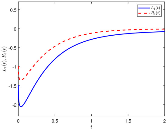
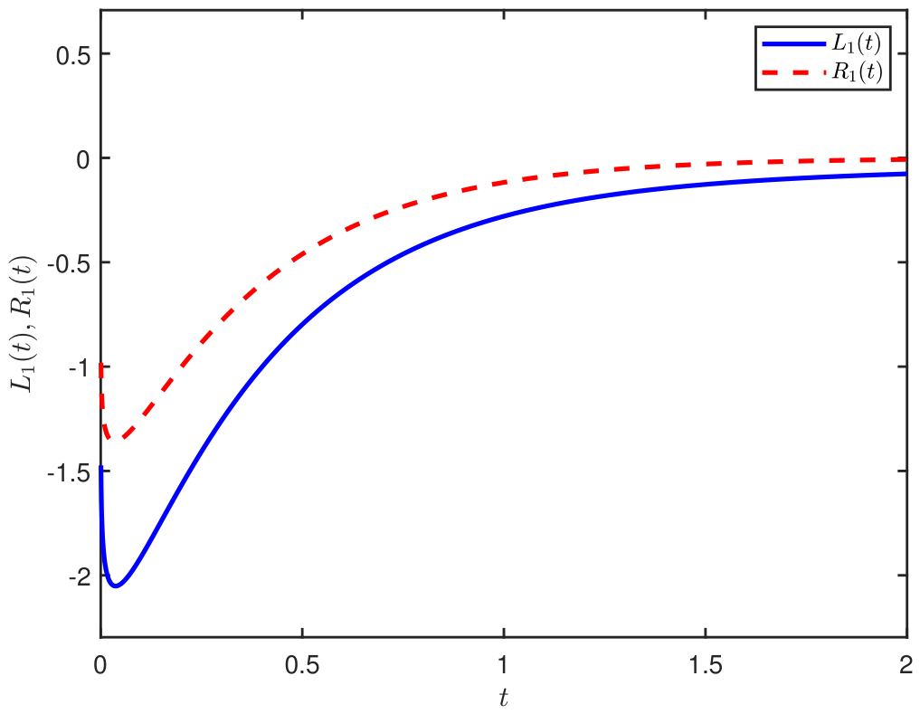
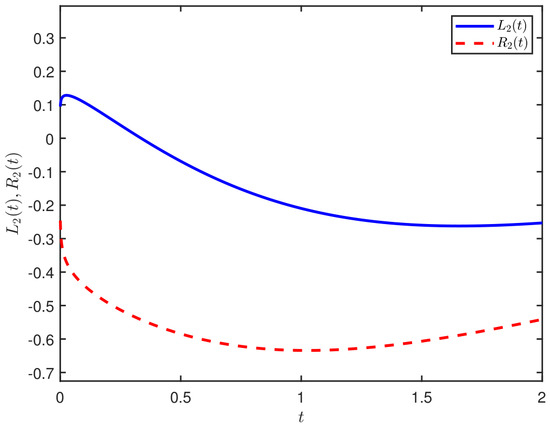
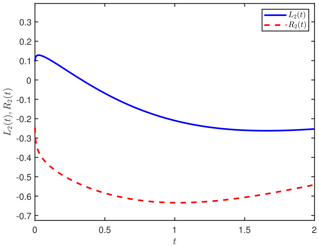
Three scalar examples are used to illustrate the continuous fractional inequalities. The first example satisfies the admissible convex condition. The second one corresponds to the concave reverse case. The third one shows that convexity in x alone is not sufficient. For the numerical illustrations below, we set $\alpha =0.9$ and $x\left(t\right)=e^{-t}$. To compare the two sides of the corresponding fractional inequality, define

$$L_i\left(t\right)={}_0{}^{C}D_t^{0.9}{V}_i(t,x\left(t\right)),R_i\left(t\right)=V_{i,x}(t,x\left(t\right)){}_0{}^{C}D_t^{0.9}x\left(t\right),i=1,2,3.$$

Example 1 

(Convex admissible case). Let $V_1(t,x)=e^{-t}{x}^2$. Then $V_1(t,·)$ is convex and $V_1(t,x\left(s\right))-V_1(s,x\left(s\right))=(e^{-t}-e^{-s})e^{-2s}<0$ for $0\le s<t$. Hence, Theorem 1 applies.

The numerical comparison in Figure 1 gives $L_1\left(t\right)\le R_1\left(t\right)$ on the computed interval, in agreement with Theorem 1.

Figure 1. Comparison of $L_1\left(t\right)$ and $R_1\left(t\right)$ in the continuous convex admissible case.

Example 2 

(Concave reverse case). Let $V_2(t,x)=(1+t)\ln (1+x)$, $x>-1$. Then $V_2(t,·)$ is concave and $V_2(t,x\left(s\right))-V_2(s,x\left(s\right))=(t-s)\ln (1+e^{-s})>0$. Hence, Theorem 2 applies.

Figure 2 shows that the reverse inequality $L_2\left(t\right)\ge R_2\left(t\right)$ on the computed interval, in agreement with Theorem 2.

Figure 2. Comparison of $L_2\left(t\right)$ and $R_2\left(t\right)$ in the continuous concave reverse case.

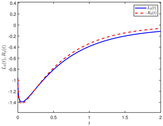
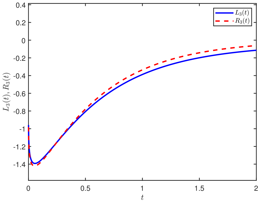
Example 3 

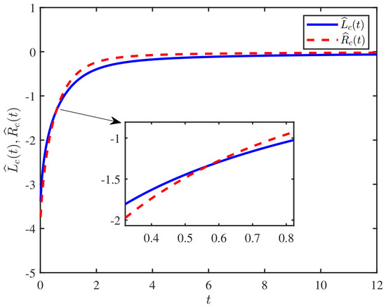
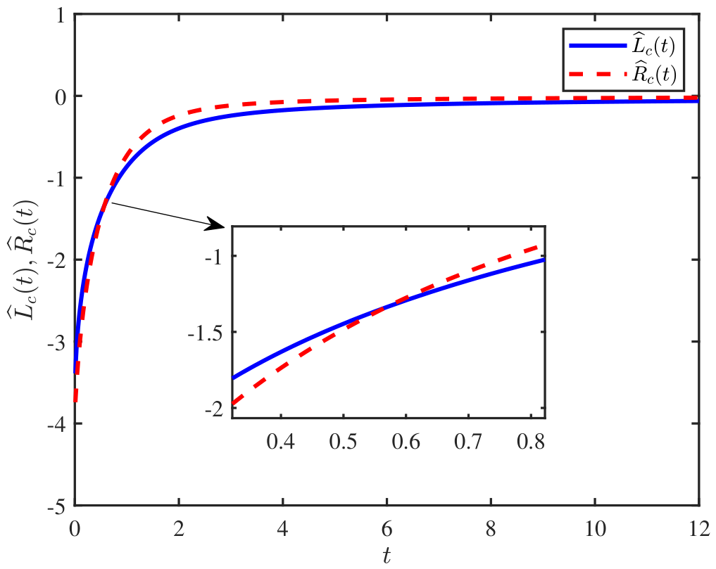
(Failure under convexity alone). Let $V_3(t,x)=(1+\epsilon t)x^2$, where $\epsilon =0.05$. Then $V_3(t,·)$ is convex, but $V_3(t,x\left(s\right))-V_3(s,x\left(s\right))=\epsilon (t-s)e^{-2s}>0$ for $0\le s<t$. Thus, the ordering condition in Theorem 1 is violated.

In Figure 3, $L_3\left(t\right)>R_3\left(t\right)$ on an initial subinterval, so the expected inequality $L_3\left(t\right)\le R_3\left(t\right)$ fails even though $V_3(t,·)$ is convex. This indicates that convexity with respect to x alone is insufficient for the continuous fractional chain-type inequality.

Figure 3. Comparison of $L_3\left(t\right)$ and $R_3\left(t\right)$ in the continuous convex non-admissible case.

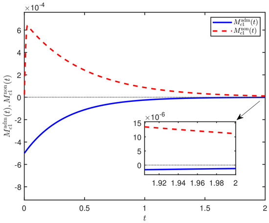
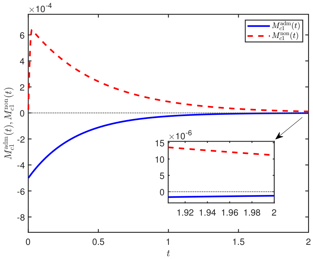
To identify the mechanism behind the failure, the historical residual used in the proof is evaluated. For a time-varying function $V_i(t,x)$, define

$$G_{i,t}\left(s\right)=V_i(t,x\left(t\right))-V_i(s,x\left(s\right))-V_{ix}(t,x\left(t\right))[x\left(t\right)-x\left(s\right)],0\le s<t.$$

The corresponding maximum residuals for the admissible and non-admissible convex cases are

$$M_{c1}^{\mathrm{adm}}\left(t\right)=\underset{0\le s<t}{\max }{G}_{1,t}\left(s\right),M_{c1}^{\mathrm{non}}\left(t\right)=\underset{0\le s<t}{\max }{G}_{3,t}\left(s\right).$$

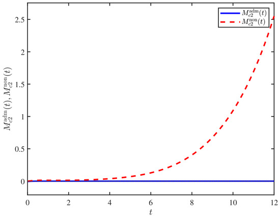
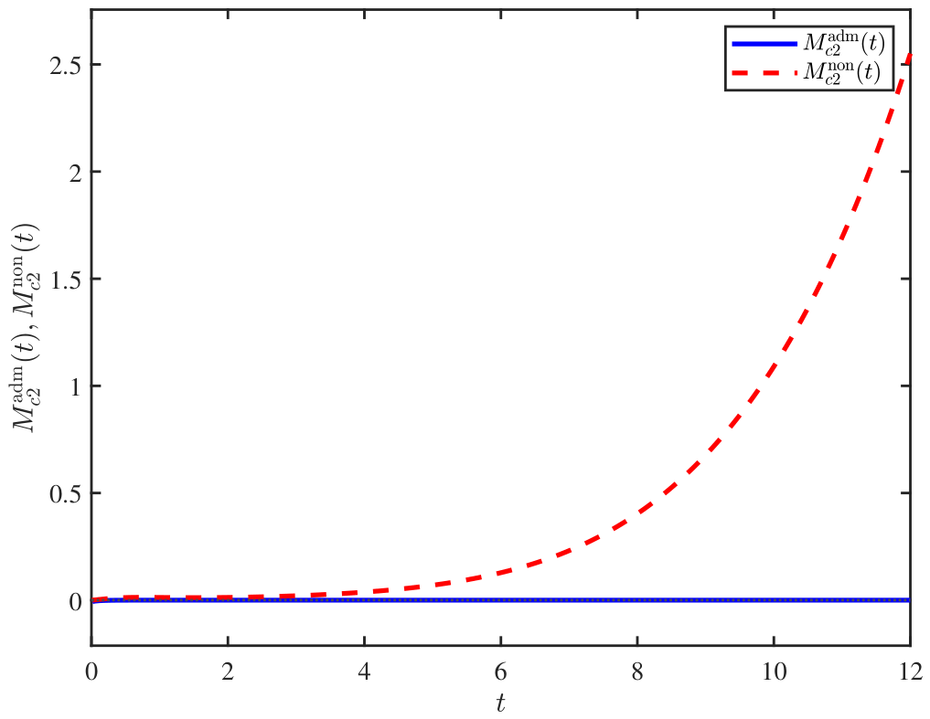
Figure 4 shows that $M_{c1}^{\mathrm{adm}}\left(t\right)\le 0$ on the computed interval, meaning that the historical residual remains nonpositive and the ordering condition is satisfied. In contrast, $M_{c1}^{\mathrm{non}}\left(t\right)>0$ throughout the computed interval, meaning that a positive historical residual exists for each current time t. Therefore, the ordering condition is persistently violated in the non-admissible case. Thus, the failure in Example 3 is caused by the loss of the historical residual sign condition, not by the loss of convexity.

Figure 4. Historical residual maximum comparison between the continuous admissible and non-admissible convex cases.

4. Discrete Nabla Fractional Inequalities

The discrete case has the same supporting-hyperplane mechanism as the continuous one, but the memory is accumulated differently. The continuous derivative uses an integral over a continuum of past states, whereas the nabla fractional difference uses a finite weighted sum over historical grid points.

4.1. Convex Case

Theorem 3 

(Discrete time-varying convex inequality). Let $0<\alpha <1$, and $D\subset {\mathbb{R}}^n$ be a convex domain. Consider a vector function $x:{\mathbb{N}}_a\to D$ and a scalar function $W:{\mathbb{N}}_a\times D\to \mathbb{R}$. Assume that $W(k,·)$ is convex for each $k\in {\mathbb{N}}_a$. If, for each fixed $k\in {\mathbb{N}}_{a+1}$,

$$W(k,x(j\left)\right)\le W(j,x(j\left)\right),j=a,a+1,\dots ,k-1,$$

(7)

then

$${}_a{}^C\nabla _k^{\alpha }W(k,x\left(k\right))\le W_x{(k,x\left(k\right))}^{\top }{}_a{}^C\nabla _k^{\alpha }x\left(k\right),k\in {\mathbb{N}}_{a+1}.$$

(8)

Proof. 

Fix $k\in {\mathbb{N}}_{a+1}$. Define

$$G_k\left(j\right)=W(k,x\left(k\right))-W(j,x\left(j\right))-W_x{(k,x\left(k\right))}^{\top }[x\left(k\right)-x\left(j\right)],a\le j\le k.$$

This residual can be decomposed as

$$\begin{array}{c}\hfill G_k\left(j\right)=\left[W(k,x\left(k\right))-W(k,x\left(j\right))-W_x{(k,x\left(k\right))}^{\top }(x\left(k\right)-x\left(j\right))\right]+\left[W(k,x(j\left)\right)-W(j,x(j\left)\right)\right].\end{array}$$

The first bracket is nonpositive by the convexity of $W(k,·)$, and the second bracket is nonpositive by Equation (7). Hence,

$$G_k\left(j\right)\le 0,j=a,a+1,\dots ,k-1,G_k\left(k\right)=0.$$

By Definition 2,

$$\begin{array}{c}\hfill {}_a{}^C\nabla _k^{\alpha }W(k,x\left(k\right))-W_x{(k,x\left(k\right))}^{\top }{}_a{}^C\nabla _k^{\alpha }x\left(k\right)=-{\displaystyle \sum _{j=a+1}^k}{\displaystyle \frac{{(k-j+1)}^{\overline{-\alpha }}}{\Gamma (1-\alpha )}}\nabla G_k\left(j\right).\end{array}$$

Let

$$b_{k,j}={\displaystyle \frac{{(k-j+1)}^{\overline{-\alpha }}}{\Gamma (1-\alpha )}},j=a+1,\dots ,k.$$

Then

$$-{\displaystyle \sum _{j=a+1}^k}{b}_{k,j}\nabla G_k\left(j\right)=-{\displaystyle \sum _{j=a+1}^k}{b}_{k,j}{G}_k\left(j\right)+{\displaystyle \sum _{j=a+1}^k}{b}_{k,j}{G}_k(j-1).$$

Changing the index in the second sum gives

$${\displaystyle \sum _{j=a+1}^k}{b}_{k,j}{G}_k(j-1)={\displaystyle \sum _{j=a}^{k-1}}{b}_{k,j+1}{G}_k\left(j\right).$$

Therefore,

$$\begin{array}{cc}\hfill -{\displaystyle \sum _{j=a+1}^k}{b}_{k,j}\nabla G_k\left(j\right)=& b_{k,a+1}{G}_k\left(a\right)+{\displaystyle \sum _{j=a+1}^{k-1}}(b_{k,j+1}-b_{k,j})G_k\left(j\right)-b_{k,k}{G}_k\left(k\right).\hfill \end{array}$$

Consequently,

$$\begin{array}{cc}\hfill & {}_a{}^C\nabla _k^{\alpha }W(k,x\left(k\right))-W_x{(k,x\left(k\right))}^{\top }{}_a{}^C\nabla _k^{\alpha }x\left(k\right)\hfill \\ \hfill =& b_{k,a+1}{G}_k\left(a\right)+{\displaystyle \sum _{j=a+1}^{k-1}}(b_{k,j+1}-b_{k,j})G_k\left(j\right)-b_{k,k}{G}_k\left(k\right).\hfill \end{array}$$

(9)

Since $G_k\left(k\right)=0$, it remains to compute the weights. By the identity

$${(z-1)}^{\overline{\mu }}-z^{\overline{\mu }}=-\mu z^{\overline{\mu -1}},$$

with $z=k-j+1$ and $\mu =-\alpha$, one obtains

$$b_{k,j+1}-b_{k,j}={\displaystyle \frac{{(k-j)}^{\overline{-\alpha }}-{(k-j+1)}^{\overline{-\alpha }}}{\Gamma (1-\alpha )}}=-{\displaystyle \frac{{(k-j+1)}^{\overline{-\alpha -1}}}{\Gamma (-\alpha )}}.$$

Thus, Equation (9) becomes

$$\begin{array}{cc}\hfill & {}_a{}^C\nabla _k^{\alpha }W(k,x\left(k\right))-W_x{(k,x\left(k\right))}^{\top }{}_a{}^C\nabla _k^{\alpha }x\left(k\right)\hfill \\ \hfill =& {\displaystyle \frac{{(k-a)}^{\overline{-\alpha }}}{\Gamma (1-\alpha )}}{G}_k\left(a\right)-{\displaystyle \sum _{j=a+1}^{k-1}}{\displaystyle \frac{{(k-j+1)}^{\overline{-\alpha -1}}}{\Gamma (-\alpha )}}{G}_k\left(j\right).\hfill \end{array}$$

(10)

For $0<\alpha <1$,

$${\displaystyle \frac{{(k-a)}^{\overline{-\alpha }}}{\Gamma (1-\alpha )}}>0,-{\displaystyle \frac{{(k-j+1)}^{\overline{-\alpha -1}}}{\Gamma (-\alpha )}}>0.$$

Together with $G_k\left(j\right)\le 0$, $j=a,a+1,\dots ,k-1$, this implies that the right-hand side of Equation (10) is nonpositive. Therefore, Equation (8) follows.  □

Remark 5. 

Formula Equation (10) is the discrete counterpart of Equation (4), but the two expressions have different memory structures. In the continuous case, the residual $G_t\left(s\right)$ is integrated over the interval $s\in [t_0,t]$. In the nabla case, only the finite collection of historical grid points $j=a,a+1,\dots ,k-1$ enters the memory sum. Therefore, condition Equation (7) is imposed only on the historical states that actually appear in the nabla fractional difference. It is weaker than requiring

$$W(k,\xi )\le W(j,\xi ),\forall \xi \in D,j<k.$$

This point is important in applications, because the required ordering is pathwise rather than a global monotonicity condition on the whole state space.

Remark 6. 

The separable product form $W(k,x(k\left)\right)=\varphi \left(k\right)U\left(x\right(k\left)\right)$, with $U\left(x\right(j\left)\right)\ge 0$ for all historical indices $j\in {\mathbb{N}}_a$, $j<k$, is a common elementary structure in discrete fractional Lyapunov analysis. In this case, condition Equation (7) becomes $\varphi \left(k\right)U\left(x\right(j\left)\right)\le \varphi \left(j\right)U\left(x\right(j\left)\right)$, $j<k$, which is automatically satisfied if $\varphi \left(k\right)$ is nonincreasing. Thus, Theorem 3 includes the usual product-form nabla fractional inequality as a special case [19]. This also clarifies why a positive time factor cannot be moved out of a fractional difference without a monotonicity condition. The difference operator retains weighted contributions from previous grid points. For a general nonseparable time-varying function $W(k,x)$, this sign is instead characterized by the discrete historical ordering condition.

4.2. Concave Case

Theorem 4 

(Discrete time-varying concave inequality). Let $0<\alpha <1$, and $D\subset {\mathbb{R}}^n$ be a convex domain. Consider a vector function $x:{\mathbb{N}}_a\to D$ and a scalar function $W:{\mathbb{N}}_a\times D\to \mathbb{R}$. Assume that $W(k,·)$ is concave for each $k\in {\mathbb{N}}_a$. If, for each fixed $k\in {\mathbb{N}}_{a+1}$,

$$W(k,x(j\left)\right)\ge W(j,x(j\left)\right),j=a,a+1,\dots ,k-1,$$

(11)

then

$${}_a{}^C\nabla _k^{\alpha }W(k,x\left(k\right))\ge W_x{(k,x\left(k\right))}^{\top }{}_a{}^C\nabla _k^{\alpha }x\left(k\right),k\in {\mathbb{N}}_{a+1}.$$

(12)

Proof. 

For the residual $G_k\left(j\right)$ used in the proof of Theorem 3, the concavity of $W(k,·)$ and Equation (11) give $G_k\left(j\right)\ge 0$ for $j=a,a+1,\dots ,k-1$. Since the weights in Equation (10) are positive, Equation (12) follows.  □

Remark 7. 

For a general time-varying function $W(k,x(k\left)\right)$, reversing the ordering condition alone does not reverse the nabla chain inequality. As in the continuous case, the sign of the supporting residual also depends on the curvature of $W(k,·)$. Therefore, the reverse inequality follows from the combination of reversed historical ordering condition Equation (11) and concavity with respect to x. This distinction is essential in the discrete case because every historical grid point contributes to the current fractional difference through a positive weight.

4.3. Simulation Study

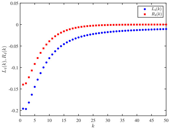
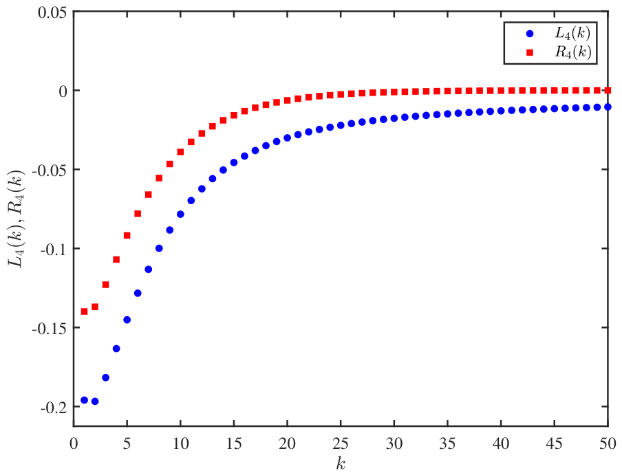
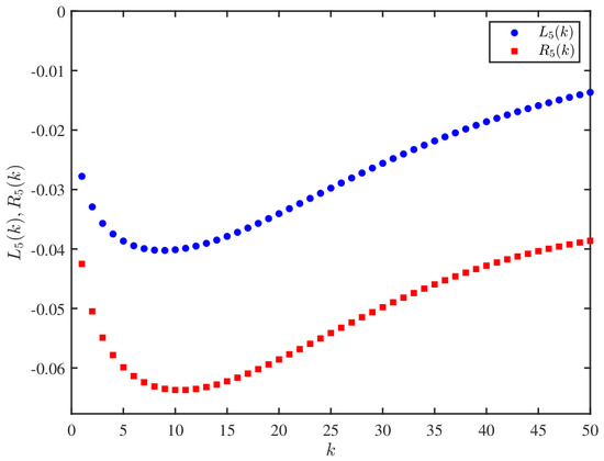
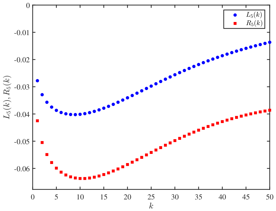
Three scalar examples are used to illustrate the discrete nabla fractional inequalities. To distinguish them from the continuous examples, the quantities are denoted by $L_i\left(k\right)={}_0{}^C\nabla _k^{\alpha }{W}_i(k,x\left(k\right))$ and $R_i\left(k\right)=W_{i,x}(k,x\left(k\right)){}_0{}^C\nabla _k^{\alpha }x\left(k\right)$, $i=4,5,6$. The numerical parameters are $a=0$, $\alpha =0.8$, and $x\left(k\right)={0.92}^k$.

Example 4 

(Convex admissible case). Let $W_4(k,x)={\rho }^k{x}^2$, where $\rho =0.95$. Then $W_4(k,·)$ is convex and $W_4(k,x\left(j\right))-W_4(j,x\left(j\right))=({\rho }^k-{\rho }^j)x^2\left(j\right)\le 0$ for $0\le j<k$. Hence, Theorem 3 applies.

The gridwise comparison in Figure 5 gives $L_4\left(k\right)\le R_4\left(k\right)$ for the computed values of k, in agreement with Theorem 3.

Figure 5. Comparison of $L_4\left(k\right)$ and $R_4\left(k\right)$ in the discrete convex admissible case.

Example 5 

(Concave reverse case). Let $W_5(k,x)={\sigma }^k\ln (1+x)$, where $\sigma =1.02$ and $x>-1$. Then $W_5(k,·)$ is concave. Since $x\left(j\right)>0$, $W_5(k,x\left(j\right))-W_5(j,x\left(j\right))=({\sigma }^k-{\sigma }^j)\ln (1+x\left(j\right))\ge 0$ for $0\le j<k$. Thus, Theorem 4 applies.

Figure 6 shows that the reverse inequality $L_5\left(k\right)\ge R_5\left(k\right)$ holds on the computed grid, in agreement with Theorem 4.

Figure 6. Comparison of $L_5\left(k\right)$ and $R_5\left(k\right)$ in the discrete concave reverse case.

Example 6 

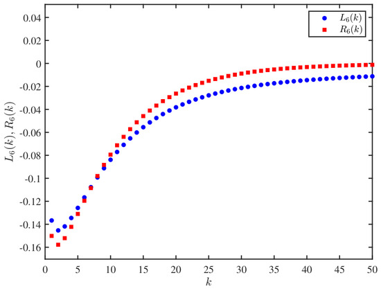
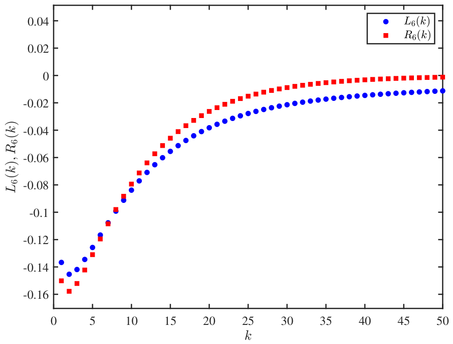
(Failure under convexity alone). Let $W_6(k,x)={\rho }_u^k{x}^2$, where ${\rho }_u=1.02$. Although $W_6(k,·)$ is convex, condition Equation (7) is violated because $W_6(k,x\left(j\right))-W_6(j,x\left(j\right))=({\rho }_u^k-{\rho }_u^j)x^2\left(j\right)>0$ for $0\le j<k$ and $x\left(j\right)\ne 0$. At $k=1$, ${}_0{}^C\nabla _1^{\alpha }q\left(1\right)=q\left(1\right)-q\left(0\right)$. Hence,

$$L_6\left(1\right)-R_6\left(1\right)={\rho }_u(2\times 0.92-{0.92}^2)-1=0.013472>0.$$

Therefore,

$${}_0{}^C\nabla _1^{\alpha }{W}_6(1,x\left(1\right))>W_{6x}(1,x\left(1\right)){}_0{}^C\nabla _1^{\alpha }x\left(1\right).$$

In Figure 7, the first grid point already gives $L_6\left(1\right)>R_6\left(1\right)$, and hence the expected inequality $L_6\left(k\right)\le R_6\left(k\right)$ is not satisfied. This indicates that convexity with respect to x alone is insufficient for the discrete fractional chain-type inequality.

Figure 7. Comparison of $L_6\left(k\right)$ and $R_6\left(k\right)$ in the discrete convex non-admissible case.

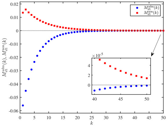
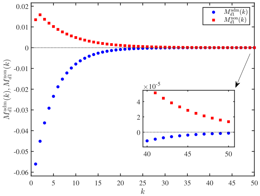
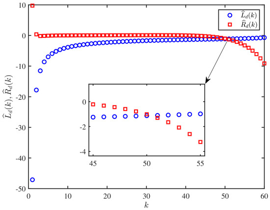
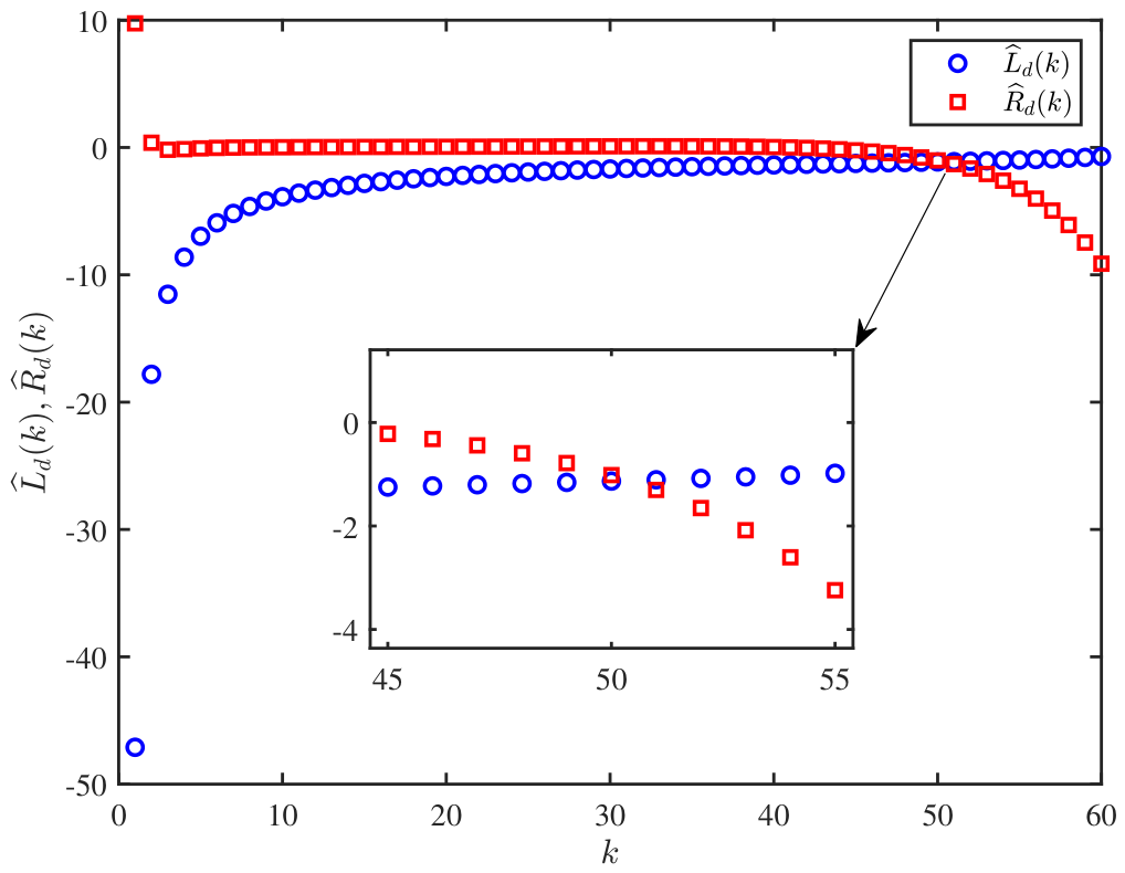
The same residual diagnostic is used in the discrete case. For a time-varying function $W_i(k,x)$, define

$$G_{i,k}\left(j\right)=W_i(k,x\left(k\right))-W_i(j,x\left(j\right))-W_{ix}(k,x\left(k\right))[x\left(k\right)-x\left(j\right)],0\le j<k.$$

For Examples 4 and 6, set

$$M_{d1}^{\mathrm{adm}}\left(k\right)=\underset{0\le j<k}{\max }{G}_{4,k}\left(j\right),M_{d1}^{\mathrm{non}}\left(k\right)=\underset{0\le j<k}{\max }{G}_{6,k}\left(j\right).$$

Figure 8 shows that $M_{d1}^{\mathrm{adm}}\left(k\right)\le 0$ on the computed grid, meaning that the discrete historical residuals remain nonpositive over all past grid points and condition Equation (7) is satisfied. In contrast, $M_{d1}^{\mathrm{non}}\left(k\right)>0$ on the computed grid, meaning that a positive residual exists over the past grid points for each current index k. Hence, the ordering condition is persistently violated in the non-admissible case. This explains why the discrete inequality may fail even though convexity with respect to x is retained.

Figure 8. Historical residual maximum comparison between the discrete admissible and non-admissible convex cases.

Remark 8. 

The need for a monotonicity or historical ordering condition is not specific to the fractional definition used in this paper. It is a general consequence of fractional memory. For a continuous fractional derivative, the product form $\varphi \left(t\right)U\left(x\right(t\left)\right)$ generates historical terms involving the comparison between $\varphi \left(t\right)$ and $\varphi \left(s\right)$, $s<t$. Therefore, a nonincreasing time factor provides a sufficient condition for the historical contribution to have the desired sign. For a discrete fractional difference, the same mechanism appears as a weighted sum over the past grid points, where the sign is determined by the comparisons between $\varphi \left(k\right)$ and $\varphi \left(j\right)$, $j<k$. Similar monotonicity requirements appear for Caputo-, Riemann–Liouville-, and Grünwald–Letnikov-type operators in both continuous and discrete settings [19].

5. Applications to Time-Varying Lyapunov Functions

Two examples are given to illustrate how the proposed inequalities are used for time-varying Lyapunov functions. In both examples, the original admissible Lyapunov function is compared with a positive time-scaled version. The comparison is used to show that historical ordering is not preserved under an arbitrary positive time scaling.

5.1. Continuous Example

Example 7. 

Consider

$$\left\{\begin{array}{cc}\hfill {}_0{}^{C}D_t^{\alpha }{x}_1\left(t\right)& =-x_1\left(t\right)-(1+e^{-t})x_2\left(t\right),\hfill \\ \hfill {}_0{}^{C}D_t^{\alpha }{x}_2\left(t\right)& =x_1\left(t\right)-x_2\left(t\right),\hfill \\ \hfill {}_0{}^{C}D_t^{\alpha }{x}_3\left(t\right)& =-x_3\left(t\right).\hfill \end{array}\right.$$

(13)

Following [20], choose

$$V_c(t,x)=x_1^2+(1+e^{-t})x_2^2+x_3^2.$$

Since $1+e^{-t}$ is positive and nonincreasing, $V_c(t,x\left(s\right))-V_c(s,x\left(s\right))=(e^{-t}-e^{-s})x_2^2\left(s\right)\le 0$ for $0\le s<t$. Moreover, $V_c(t,·)$ is convex. Hence, Theorem 1 gives

$${}_0{}^{C}D_t^{\alpha }{V}_c(t,x\left(t\right))\le V_{cx}{(t,x\left(t\right))}^{\top }{}_0{}^{C}D_t^{\alpha }x\left(t\right).$$

Along Equation (13),

$$\begin{array}{cc}\hfill V_{cx}{(t,x\left(t\right))}^{\top }{}_0{}^{C}D_t^{\alpha }x\left(t\right)& =2x_1[-x_1-(1+e^{-t})x_2]+2(1+e^{-t})x_2(x_1-x_2)-2x_3^2\hfill \\ & =-2V_c(t,x\left(t\right)).\hfill \end{array}$$

Since $1\le 1+e^{-t}\le 2$, one has ${\parallel x\parallel }^2\le V_c(t,x)\le 2{\parallel x\parallel }^2$. Moreover, ${}_0{}^{C}D_t^{\alpha }{V}_c(t,x\left(t\right))\le -2V_c(t,x\left(t\right))\le -2{\parallel x\left(t\right)\parallel }^2$. It follows from the Mittag–Leffler stability criterion in [25] that the zero solution of Equation (13) is Mittag–Leffler-stable.

Now define ${\widehat{V}}_c(t,x)={\eta }_c\left(t\right)V_c(t,x)$, where ${\eta }_c\left(t\right)=e^{0.35t}$. For each fixed t, ${\widehat{V}}_c(t,·)$ remains convex and positive definite. However, since ${\eta }_c\left(t\right)$ is increasing, the historical ordering ${\widehat{V}}_c(t,x\left(s\right))\le {\widehat{V}}_c(s,x\left(s\right))$, $0\le s<t$, is not generally satisfied. Therefore, Theorem 1 cannot be applied to ${\widehat{V}}_c$.

For the numerical illustration, we set $\alpha =0.8$ and $x\left(0\right)={(0.8,-0.7,0.6)}^{\top }$. Define

$$L_c\left(t\right)={}_0{}^{C}D_t^{\alpha }{V}_c(t,x\left(t\right)),R_c\left(t\right)=V_{cx}{(t,x\left(t\right))}^{\top }{}_0{}^{C}D_t^{\alpha }x\left(t\right),$$

and define ${\widehat{L}}_c\left(t\right)$, ${\widehat{R}}_c\left(t\right)$ similarly for ${\widehat{V}}_c$.

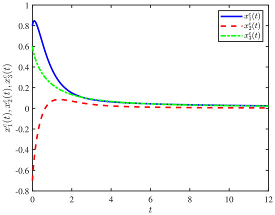
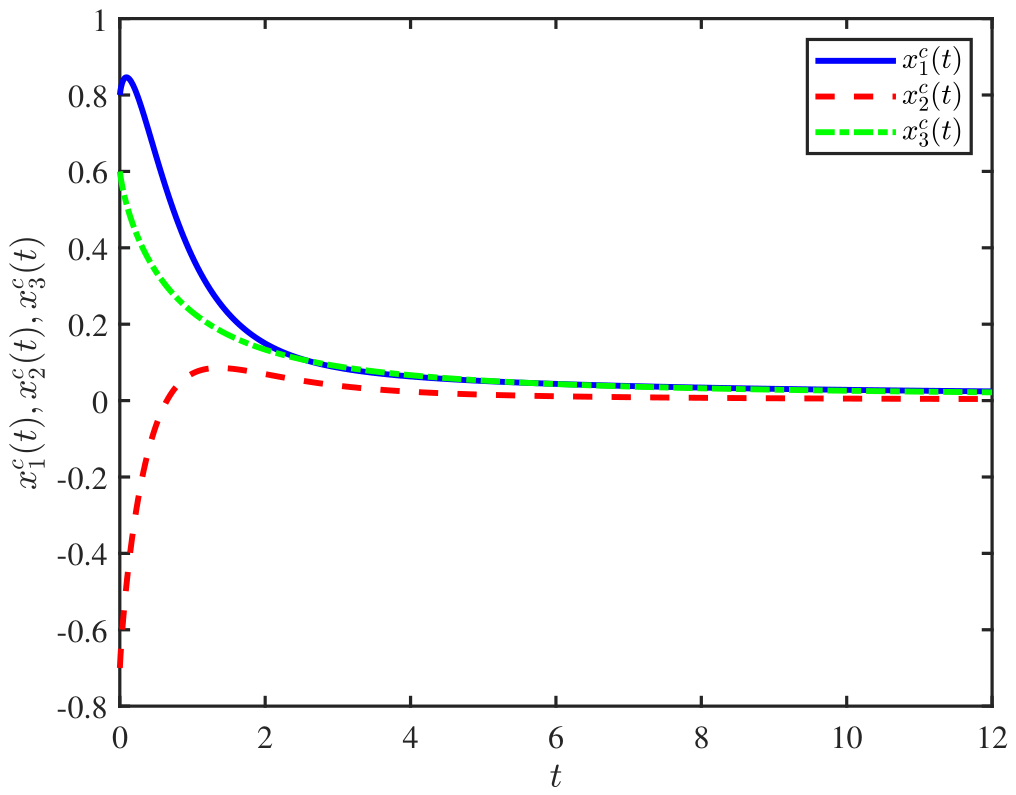
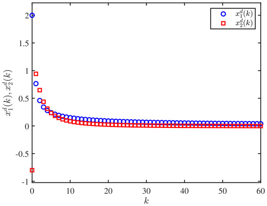
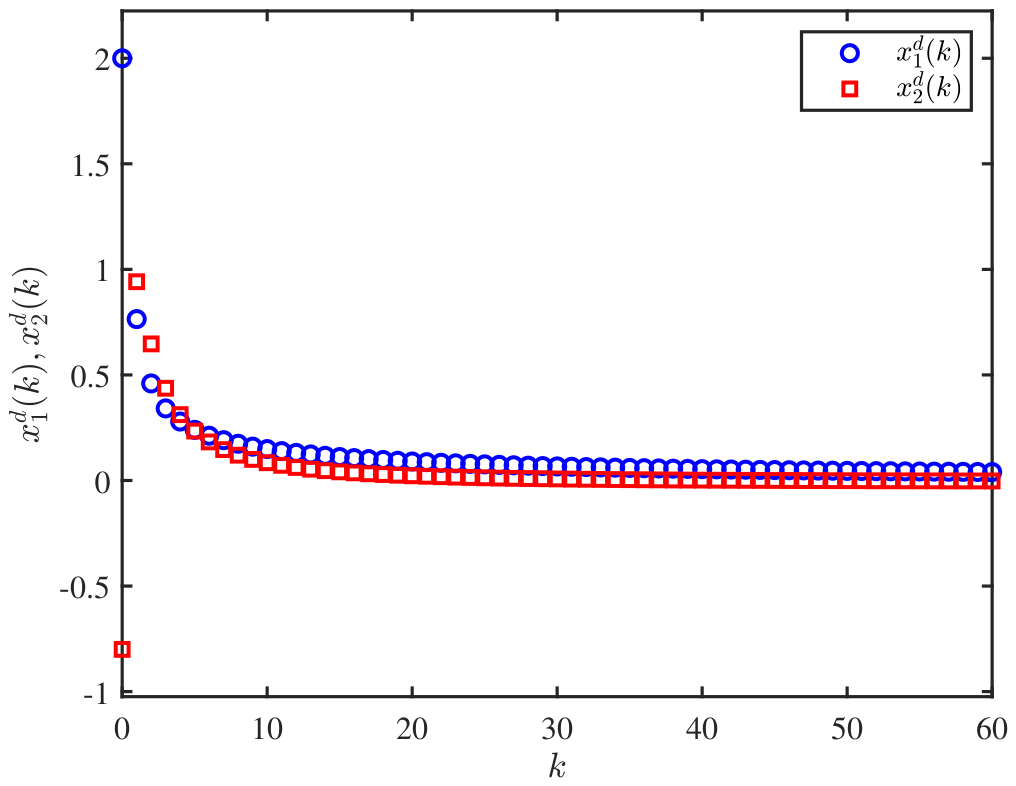
Figure 9 gives the state trajectories of the continuous fractional-order system, which are used to evaluate the Lyapunov inequalities along the solution. For the admissible Lyapunov function, Figure 10 shows that $L_c\left(t\right)\le R_c\left(t\right)$ on the computed interval, in agreement with Theorem 1. In contrast, Figure 11 shows that the same inequality may fail after a positive time scaling. This indicates that convexity and positive definiteness are not sufficient without the historical ordering condition.

Figure 9. State trajectories of the continuous fractional-order system in Equation (13).

Figure 10. Comparison of $L_c\left(t\right)$ and $R_c\left(t\right)$ for the admissible continuous Lyapunov function $V_c$.

Figure 11. Comparison of ${\widehat{L}}_c\left(t\right)$ and ${\widehat{R}}_c\left(t\right)$ for the scaled continuous function ${\widehat{V}}_c$.

For the application example, the same continuous residual diagnostic is applied to $V_c$ and to its scaled version ${\widehat{V}}_c$. Define

$$M_{c2}^{\mathrm{adm}}\left(t\right)=\underset{0\le s<t}{\max }\left\{V_c(t,x\left(t\right))-V_c(s,x\left(s\right))-V_{cx}{(t,x\left(t\right))}^{\top }[x\left(t\right)-x\left(s\right)]\right\},$$

and

$$M_{c2}^{\mathrm{non}}\left(t\right)=\underset{0\le s<t}{\max }\left\{{\widehat{V}}_c(t,x\left(t\right))-{\widehat{V}}_c(s,x\left(s\right))-{\widehat{V}}_{cx}{(t,x\left(t\right))}^{\top }[x\left(t\right)-x\left(s\right)]\right\}.$$

As shown in Figure 12, $M_{c2}^{\mathrm{adm}}\left(t\right)\le 0$, while $M_{c2}^{\mathrm{non}}\left(t\right)$ becomes positive. Thus, the positive time scaling destroys the historical residual condition, although ${\widehat{V}}_c(t,·)$ remains convex and positive definite for each fixed t.

Figure 12. Historical residual maximum comparison for Example 7.

5.2. Discrete Example

Example 8. 

Consider the nonautonomous nabla fractional-order system [19]

$$\left\{\begin{array}{cc}\hfill {}_0{}^C\nabla _k^{\alpha }{x}_1\left(k\right)& =-x_1\left(k\right)-h\left(k\right)x_2\left(k\right),\hfill \\ \hfill {}_0{}^C\nabla _k^{\alpha }{x}_2\left(k\right)& =3h^{-1}\left(k\right)x_1^3\left(k\right)-x_2\left(k\right),\hfill \end{array}\right.$$

(14)

where $h\left(k\right)>0$ is decreasing. Following [19], choose

$$W_d(k,x)=3x_1^4+2h^2\left(k\right)x_2^2.$$

In this example, $h\left(k\right)=1+1/(k+1)$. Then $W_d(k,x\left(j\right))-W_d(j,x\left(j\right))=2[h^2\left(k\right)-h^2\left(j\right)]x_2^2\left(j\right)\le 0$ for $0\le j<k$, and $W_d(k,·)$ is convex. By Theorem 3,

$${}_0{}^C\nabla _k^{\alpha }{W}_d(k,x\left(k\right))\le W_{dx}{(k,x\left(k\right))}^{\top }{}_0{}^C\nabla _k^{\alpha }x\left(k\right).$$

Along Equation (14),

$$\begin{array}{cc}\hfill W_{dx}{(k,x\left(k\right))}^{\top }{}_0{}^C\nabla _k^{\alpha }x\left(k\right)& =12x_1^3[-x_1-h\left(k\right)x_2]+4h^2\left(k\right)x_2[3h^{-1}\left(k\right)x_1^3-x_2]\hfill \\ & =-12x_1^4-4h^2\left(k\right)x_2^2\le -2W_d(k,x\left(k\right)).\hfill \end{array}$$

Thus, $W_d$ is an admissible time-varying Lyapunov function, and the zero solution of Equation (14) is asymptotically stable.

Now define ${\widehat{W}}_d(k,x)={\eta }_d\left(k\right)W_d(k,x)$, where ${\eta }_d\left(k\right)={1.2}^k$. For each fixed k, ${\widehat{W}}_d(k,·)$ remains convex and positive definite. However, since ${\eta }_d\left(k\right)$ is increasing, the historical ordering

$${\widehat{W}}_d(k,x\left(j\right))\le {\widehat{W}}_d(j,x\left(j\right)),0\le j<k,$$

is not generally satisfied. Hence, Theorem 3 cannot be applied to ${\widehat{W}}_d$.

For the numerical illustration, we set $\alpha =0.7$ and $x\left(0\right)={(2,-0.8)}^{\top }$. Define

$$L_d\left(k\right)={}_0{}^C\nabla _k^{\alpha }{W}_d(k,x\left(k\right)),R_d\left(k\right)=W_{dx}{(k,x\left(k\right))}^{\top }{}_0{}^C\nabla _k^{\alpha }x\left(k\right),$$

and define ${\widehat{L}}_d\left(k\right)$, ${\widehat{R}}_d\left(k\right)$ similarly for ${\widehat{W}}_d$.

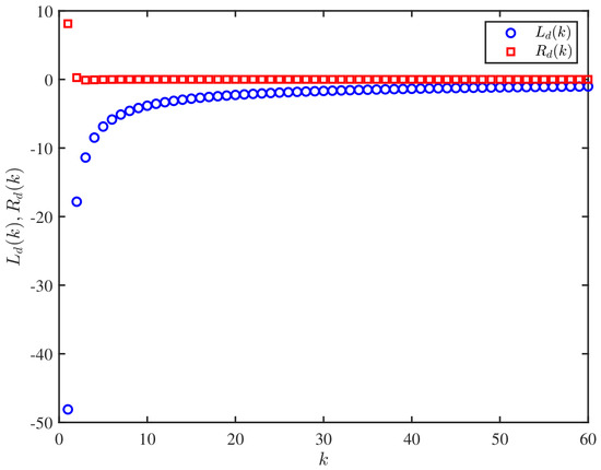
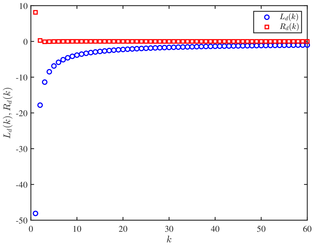
Figure 13 gives the state trajectories of the discrete fractional-order system. Figure 14 shows that the admissible Lyapunov function satisfies $L_d\left(k\right)\le R_d\left(k\right)$ on the computed grid, in agreement with Theorem 3. By contrast, Figure 15 shows that the positive time-scaled function may violate the same inequality. This illustrates the role of the discrete historical ordering condition in guaranteeing the fractional inequality.

Figure 13. State trajectories of the discrete nabla fractional-order system in Equation (14).

Figure 14. Comparison of $L_d\left(k\right)$ and $R_d\left(k\right)$ for the admissible discrete Lyapunov function $W_d$.

Figure 15. Comparison of ${\widehat{L}}_d\left(k\right)$ and ${\widehat{R}}_d\left(k\right)$ for the scaled discrete function ${\widehat{W}}_d$.

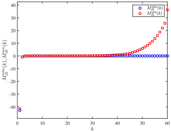
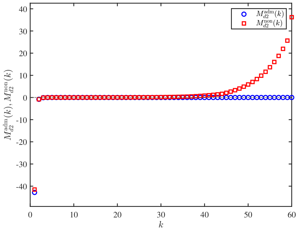
For the discrete application example, the corresponding residual diagnostic is applied to $W_d$ and ${\widehat{W}}_d$. Define

$$M_{d2}^{\mathrm{adm}}\left(k\right)=\underset{0\le j<k}{\max }\left\{W_d(k,x\left(k\right))-W_d(j,x\left(j\right))-W_{dx}{(k,x\left(k\right))}^{\top }[x\left(k\right)-x\left(j\right)]\right\},$$

and

$$M_{d2}^{\mathrm{non}}\left(k\right)=\underset{0\le j<k}{\max }\left\{{\widehat{W}}_d(k,x\left(k\right))-{\widehat{W}}_d(j,x\left(j\right))-{\widehat{W}}_{dx}{(k,x\left(k\right))}^{\top }[x\left(k\right)-x\left(j\right)]\right\}.$$

Figure 16 shows that $M_{d2}^{\mathrm{adm}}\left(k\right)\le 0$, whereas $M_{d2}^{\mathrm{non}}\left(k\right)$ becomes positive. Therefore, the failure after positive time scaling is caused by the loss of the historical residual sign condition over the discrete memory points.

Figure 16. Historical residual maximum comparison in Example 8.

6. Conclusions

This paper studied time-varying fractional Lyapunov inequalities under admissible convexity conditions. It was shown that state convexity alone is sufficient only for the time-invariant case, whereas explicitly time-varying Lyapunov functions require an additional historical ordering condition. This condition guarantees the compatibility between the current supporting hyperplane and the historical values induced by fractional memory. In the continuous Caputo case, the difference between the two sides of the inequality was represented by a weighted integral of historical residuals. In the discrete nabla Caputo case, the corresponding difference was represented by a weighted sum over past grid points. These residual representations give a unified way to characterize the continuous and discrete admissibility conditions. Reverse inequalities for concave functions were also obtained under reversed ordering conditions. The results clarify why monotonicity is essential in product-form time-varying Lyapunov functions. In particular, the product of a nonnegative convex state factor and a nonnegative nonincreasing time factor provides a simple sufficient admissible structure. The numerical examples and continuous/discrete Lyapunov applications illustrated this limitation. Positive definiteness and ordinary state convexity do not guarantee the desired fractional chain-type inequalities when the time-varying factor changes the sign of the historical residuals.

Future work will consider less conservative admissibility criteria based on weighted residual signs, as well as extensions to broader fractional operators, variable-order systems, switched nonautonomous systems, and adaptive control designs with time-varying Lyapunov weights.

References

- Brémont, J.; Régnier, L.; Barbier–Chebbah, A.; Voituriez, R.; Bénichou, O. Flips reveal the universal impact of memory on random explorations. Nat. Commun. 2026, 17, 453. [Google Scholar]
- Krejcar, O.; Namazi, H. Review of the applications of different fractional models in engineering. Appl. Math. Model. 2026, 153, 116623. [Google Scholar] [CrossRef] [Scilit]
- Luo, H.; Chen, L. From differential equation solvers to accelerated first-order methods for convex optimization. Math. Program. 2022, 195, 735–781. [Google Scholar]
- Li, C.; N’Gbo, N.; Su, F. Finite difference methods for nonlinear fractional differential equation with ψ-Caputo derivative. Phys. D Nonlinear Phenom. 2024, 460, 134103. [Google Scholar] [CrossRef] [Scilit]
- Abdel Aal, O.F.; Ozbek, N.S.; Cao, S.; Chen, Y.; Chen, Y.Q. 15 ways to apply fractional calculus in gradient descent optimization methods. IFAC-PapersOnLine 2025, 59, 19–24. [Google Scholar] [CrossRef] [Scilit]
- Hu, T.-T.; Lin, S.-Y.; Lu, Z.-C. Solution operators for Caputo-type fractional evolution equations with damping. Axioms 2026, 15, 179. [Google Scholar] [CrossRef] [Scilit]
- Tarasov, V.E. No violation of the Leibniz rule. No fractional derivative. Commun. Nonlinear Sci. Numer. Simul. 2013, 18, 2945–2948. [Google Scholar] [CrossRef] [Scilit]
- Tarasov, V.E. On chain rule for fractional derivatives. Commun. Nonlinear Sci. Numer. Simul. 2016, 30, 1–4. [Google Scholar] [CrossRef] [Scilit]
- Alikhanov, A.A. A priori estimates for solutions of boundary value problems for fractional-order equations. Differ. Equ. 2010, 46, 660–666. [Google Scholar] [CrossRef] [Scilit]
- Aguila-Camacho, N.; Duarte-Mermoud, M.A.; Gallegos, J.A. Lyapunov functions for fractional order systems. Commun. Nonlinear Sci. Numer. Simul. 2014, 19, 2951–2957. [Google Scholar] [CrossRef] [Scilit]
- Chen, W.; Dai, H.; Song, Y.; Zhang, Z. Convex Lyapunov functions for stability analysis of fractional order systems. IET Control Theory Appl. 2017, 11, 1070–1074. [Google Scholar] [CrossRef] [Scilit]
- Tuan, H.T.; Trinh, H. Stability of fractional-order nonlinear systems by Lyapunov direct method. IET Control Theory Appl. 2018, 12, 2417–2422. [Google Scholar] [CrossRef] [Scilit]
- Gomoyunov, M.I. Fractional derivatives of convex Lyapunov functions and control problems in fractional order systems. Fract. Calc. Appl. Anal. 2018, 21, 1238–1261. [Google Scholar] [CrossRef] [Scilit]
- You, X.; Dian, S.; Guo, B.; Xiao, Q.; Zhu, Y.; Liu, K. Novel finite-time adaptive fuzzy fault-tolerant control for fractional-order nonlinear systems and its applications. IEEE/CAA J. Autom. Sin. 2026, 13, 123–136. [Google Scholar] [CrossRef] [Scilit]
- Mazenc, F. Strict Lyapunov functions for time-varying systems. Automatica 2003, 39, 349–353. [Google Scholar] [CrossRef] [Scilit]
- Maghenem, M.A.; Loría, A. Strict Lyapunov functions for time-varying systems with persistency of excitation. Automatica 2017, 78, 274–279. [Google Scholar] [CrossRef] [Scilit]
- Zhou, B. Lyapunov differential equations and inequalities for stability and stabilization of linear time-varying systems. Automatica 2021, 131, 109785. [Google Scholar] [CrossRef] [Scilit]
- Lenka, B.K. Time-varying Lyapunov functions and Lyapunov stability of nonautonomous fractional order systems. Int. J. Appl. Math. 2019, 32, 111–130. [Google Scholar] [CrossRef] [Scilit]
- Wei, Y. Time-varying Lyapunov functions for nonautonomous nabla fractional order systems. ISA Trans. 2022, 126, 235–241. [Google Scholar] [CrossRef] [Scilit] [PubMed]
- Omri, F. Time-varying Lyapunov functions for nonautonomous conformable fractional-order systems. Mem. Differ. Equ. Math. Phys. 2025, 94, 131–144. [Google Scholar]
- Almutairi, O.B.; Saleh, W. Fractional Bullen-type inequalities for coordinated convex functions. Axioms 2026, 15, 292. [Google Scholar] [CrossRef] [Scilit]
- Boyd, S.; Vandenberghe, L. Convex Optimization; Cambridge University Press: Cambridge, UK, 2004. [Google Scholar]
- Kilbas, A.A.; Srivastava, H.M.; Trujillo, J.J. Theory and Applications of Fractional Differential Equations; Elsevier: Amsterdam, The Netherlands, 2006. [Google Scholar]
- Li, C.; Cai, M. Theory and Numerical Approximations of Fractional Integrals and Derivatives; SIAM: Philadelphia, PA, USA, 2019. [Google Scholar]
- Li, Y.; Chen, Y.Q.; Podlubny, I. Mittag–Leffler stability of fractional order nonlinear dynamic systems. Automatica 2009, 45, 1965–1969. [Google Scholar] [CrossRef] [Scilit]
Disclaimer/Publisher’s Note: The statements, opinions and data contained in all publications are solely those of the individual author(s) and contributor(s) and not of MDPI and/or the editor(s). MDPI and/or the editor(s) disclaim responsibility for any injury to people or property resulting from any ideas, methods, instructions or products referred to in the content. |
© 2026 by the authors. Licensee MDPI, Basel, Switzerland. This article is an open access article distributed under the terms and conditions of the Creative Commons Attribution (CC BY) license.