


Abstract
We present a novel framework for modeling reaction time distributions in the context of video games aimed at providing a performance tool to support the design of new levels. Modern games generate rich behavioral telemetry (including reaction times, success rates, and interaction patterns) that can be leveraged to understand player behavior and inform adaptive game design. Given a set of general parameters describing a newly designed level, the framework predicts the corresponding reaction time distribution, offering actionable insight during the design process. To address this problem, we employ a combination of statistical fitting via maximum likelihood estimation, weighted approximations, and Lipschitz-based estimators in Wasserstein space. This mathematical framework establishes the groundwork for future AI-based extensions, using metric-space learning to predict distributions for unseen level configurations. The methodology provides theoretical guarantees under mild mathematical assumptions, ensuring bounded estimation errors through the assumption of Lipschitz continuity. Three approaches are proposed, all grounded in a Lipschitz characterization of the metric model parameters, which embeds the vector representation of levels into the 1-Wasserstein space of reaction time distributions. The practical applicability of the framework is demonstrated on a dataset of 480 gameplay observations across 24 participants and 20 distinct trials, testing all three fitting procedures on a set of representative examples.
MSC:
62P25
1. Introduction
A substantial body of scientific literature addresses the problem of finding appropriate mathematical tools to model participant response behavior in video games, focusing on how different gaming experiences shape cognitive outcomes. For example, research has shown that while players of first-person shooters demonstrate significantly reduced reaction times, this speed may come at the cost of compromised inhibitory control compared to other gamers [1]. Furthermore, studies examining the broader relationship between gaming habits and executive functions have identified specific patterns in reaction time and working memory performance across various experience levels [2].
The potential for these digital tools to serve as cognitive interventions is supported by evidence that video game training can effectively enhance reaction time skills even among older adults [3]. Finally, the interaction between digital and physical activity indicates that both regular exercise and video game play contribute to improved response accuracy and speed in adolescents, suggesting that a balanced lifestyle can optimize motor–cognitive performance [4].
A natural and widely adopted approach is the statistical characterization of response times, which is broadly regarded as the primary tool for the mathematical description of such problems (p. 2, [5]). This perspective motivates the distributional framework developed in the present work, where each game level is represented not by a scalar performance summary, but by its full reaction time distribution. Directly related prior work can be found in a recent series of papers [6,7,8,9]. From our perspective, the central instrument is the identification of the probability distribution that best reproduces the stochastic behavior of participants. As demonstrated in the aforementioned work, response times naturally follow recognizable statistical distributions, opening the door to rigorous mathematical modeling of the response-time problem [10]. This is by no means a new research question; on the contrary, it is a classical topic in psychology and physiology for which well-established mathematical methods have long been available [11,12]. Also, from a mathematical standpoint, this issue has also been studied in technological contexts where rapid processing is required, as well as in health resource management (see e.g., [13,14,15]).
Despite the extensive literature on reaction time analysis and game analytics, existing approaches remain limited in two key aspects. First, they predominantly rely on scalar summaries, thereby discarding the rich information contained in full behavioral distributions. Second, they lack a principled mathematical framework that relates the design parameters of a game level to the resulting player response distributions. In particular, no existing methodology provides a robust metric model that relates the feature space of the level design and the space of probability distributions (for example, a Lipschitz continuous performance map), which is essential for predictive modeling with theoretical guaranties.
In our case, we approach the modeling problem from a mathematical perspective, focusing on the construction of a performance map that relates level design parameters to behavioral response distributions. The underlying premise is that, by characterizing reaction-time distributions across a sufficiently large set of existing experiences, it is possible to define similarity relations in a metric sense. This enables the systematic comparison and prediction of new levels within a unified mathematical framework.
The proposed framework is supported by an experimental study based on behavioral data collected from human participants. The dataset consists of 480 valid observations obtained from 24 players across 20 distinct game levels, with each level characterized by a sample of 24 reaction times. For each level, the empirical distribution of response times is modeled by fitting parametric families suitable for positive and skewed data, including Gamma, Weibull, and ex-Gaussian distributions. Parameters are estimated via maximum likelihood, and model selection is performed using the Akaike Information Criterion, ensuring a consistent distributional representation across all gameplay instances. This experimental component provides the empirical basis for the distributional modeling and subsequent metric analysis developed in this work. However, it is worth noting that our primary interest is to present the mathematical methodology rather than to provide a fully ready-to-use tool for video game design, which would definitely improve by expanding the dataset. Therefore, this work should be viewed as a foundational framework that can be further refined in future studies with larger groups of players.
In modern game design, procedural and data-driven methodologies increasingly rely on quantitative models of player behavior to generate and adapt gameplay content [16,17]. In particular, human reaction-time distributions provide a principled basis for calibrating core design elements such as difficulty scaling, timing constraints, and interaction dynamics. Rather than relying on fixed heuristics, designers can exploit empirical distributions of response times to define reaction windows, adjust enemy behavior, or tune user interface responsiveness in a statistically grounded manner. This is especially relevant in fast-paced genres, where gameplay balance critically depends on aligning stimulus timing with human perceptual and motor capabilities.
From a methodological standpoint, these approaches can be interpreted as instances of procedural modeling (see e.g., [18,19,20]), where game elements are generated or adapted based on measurable behavioral patterns. Reaction-time distributions naturally encode variability, learning effects, and contextual influences such as stress or multisensory stimuli, making them particularly suitable for adaptive systems. However, these approaches are typically heuristic or data-driven in nature and lack a rigorous mathematical structure that would allow for formal analysis and prediction of behavioral outcomes. This observation further motivates the distributional and metric-based perspective adopted in the present work.
Consequently, the primary contribution of this paper is the application of Lipschitz regularity requirements to evaluate the accuracy of the performance map. This map translates the design properties of a new video game level into well-behaved metric spaces (specifically the 1-Wasserstein space), which provides a natural notion of distance to measure similarity between distributions. Furthermore, we also present an alternative model based on the parametric description of these distributions and the Lipschitz extension of real-valued functions.
To conclude the introduction, we briefly review the state of the art in the main areas related to this work.
Game analytics provides a data-driven framework for understanding player behavior through the analysis of gameplay telemetry. Existing approaches typically rely on summary statistics such as completion times, success rates, or error frequencies to characterize player performance [21]. While effective in practice, these aggregated representations fail to capture the intrinsic variability in behavioral responses. The approach adopted in this work represents each gameplay instance as a probability distribution of reaction times. This perspective enables a finer characterization of player behavior and naturally supports the introduction of a metric structure on the space of game levels, which is essential for the predictive modeling framework developed in this paper.
Adaptive gameplay systems aim to adjust game difficulty in response to player performance. Dynamic Difficulty Adjustment (DDA) mechanisms typically rely on feedback-based strategies to maintain player engagement [22]. These approaches use performance indicators to modify game parameters in real time, although they are generally based on heuristic or aggregated measures of player behavior. From a modeling perspective, the framework proposed in this work can be interpreted as a distributional extension of adaptive difficulty schemes. By representing player responses through probability distributions, it becomes possible to compare gameplay instances within a metric space and to predict the behavioral outcome of new levels. This provides a principled foundation for adaptive design strategies with explicit mathematical structure.
While most game-analytic methods rely on scalar performance indicators, several areas of statistics and machine learning consider probability distributions as primary data objects. In particular, optimal transport theory provides a natural framework for comparing such distributions via Wasserstein distances [23]. In this work, we adopt a distributional representation of gameplay stimuli, where each level is characterized by its reaction-time distribution. This perspective induces a metric structure on the space of game instances, enabling comparison, interpolation, and prediction of behavioral features for new stimuli based on their similarity to previously observed data.
From a practical game design perspective, the ability to predict full reaction-time distributions for unseen level configurations provides actionable utility across several core areas of game production. Rather than relying on simple scalar metrics like mean response times, which obscure behavioral variance, the predicted probability densities allow designers to perform precise response-window calibration to guarantee accessibility across diverse player skill tiers. Furthermore, these distributions enable automated difficulty adjustment and systematic level comparison by identifying unexpected performance bottlenecks or learning curves prior to costly playtesting phases. Finally, by mapping the structural parameters of a level to cognitive performance profiles, this framework establishes a stable, mathematically bounded foundation for adaptive content generation, allowing game engines to dynamically tune features in real-time to preserve the player’s psychological state of flow.
2. Recent AI Approaches Related to Distributional Learning and Game Analytics
Recent advances in machine learning have led to the development of models in which the fundamental objects are probability distributions rather than scalar observations. This perspective has motivated a growing body of work on supervised learning problems where inputs, outputs, or both are distribution-valued. In these settings, the geometry of the space of probability measures plays a central role, and optimal transport theory provides a natural framework for defining distances and regression operators via Wasserstein metrics [23].
Several recent contributions focus on regression models defined directly in Wasserstein space. For instance, ref. [24] studies distribution-to-distribution regression models and develops tractable formulations for Gaussian measures, exploiting the geometric structure of Wasserstein space to construct interpretable mappings between distributions. More flexible approaches have been proposed in the context of nonparametric and neural models. Neural Local Wasserstein Regression [25] introduces a framework based on locally defined optimal transport maps, avoiding the distortions associated with global linear approximations and enabling more accurate modeling of distributional relationships.
Other works extend classical machine learning paradigms to distribution-valued data. Wasserstein Gradient Boosting [26] generalizes boosting methods by interpreting updates as gradient steps in Wasserstein space, allowing prediction targets to be probability measures. Active learning strategies have also been adapted to this setting: ref. [27] proposes a framework combining representativity and uncertainty criteria for regression tasks where observations are distributions. In parallel, kernel-based approaches to distribution regression provide statistical guarantees for learning from empirical measures derived from sampled data [28].
From an application perspective, video games constitute a natural domain for these methodologies due to the availability of large-scale behavioral data. Recent surveys [29] highlight the increasing use of artificial intelligence techniques in games, including reinforcement learning, procedural content generation, and player modeling. In particular, mathematical and machine learning models that use combinations of regression, classification, and reinforcement learning techniques have been widely proposed to analyze the dynamics of the game [30,31]. The framework proposed in this paper lies at the intersection of these research directions. We model gameplay stimuli as probability distributions and exploit the geometry of Wasserstein space to compare behavioral responses across tests. This representation induces a metric structure on the set of stimuli and enables the prediction of features of new instances through regression in distribution space. The resulting approach connects distributional machine learning, optimal transport, and game analytics within a unified mathematical framework.
3. Distributional Fitting of Response Times per Trial
The experimental framework was developed keeping professional game design requirements in mind. To isolate the core stimulus-response cycle that drives every video game, we designed the levels to be as streamlined and simple as possible.
The data captured during these sessions is described in Table 1. It is important to note that all participant data has been fully anonymized. During the initial acquisition phase, we recorded a total of 20 complete playthroughs.
Table 1.
Game Data Breakdown.
Thus, the analyzed dataset consists of 480 valid observations, corresponding to 24 participants across 20 distinct trials (levels). Since each level contains 24 response times, the fitting process was conducted independently for each trial based on its empirical sample. A sample of how the raw data is organized can be found in Appendix A.
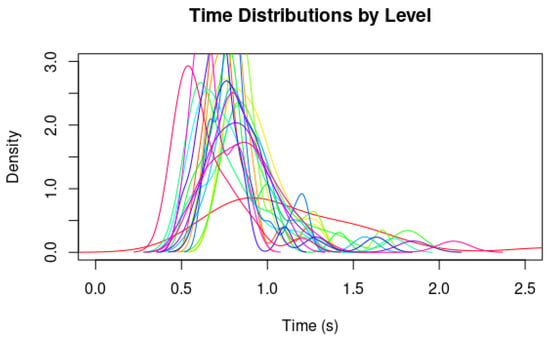
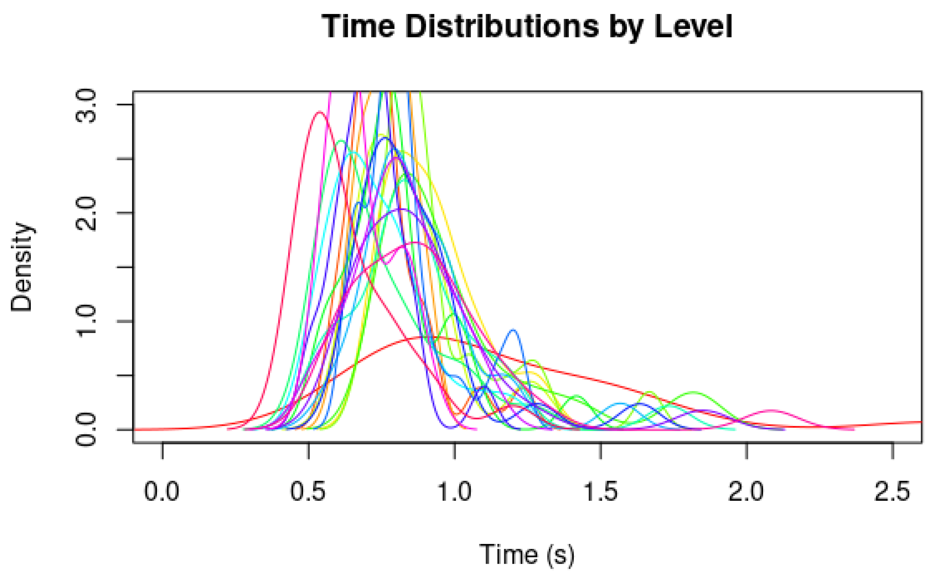
Figure 1 represents the response-times data as continuous functions for the levels considered. As observed, although they exhibit meaningful differences, they remain broadly comparable.
Figure 1.
Joint representation of the 20 considered levels. Each of the 20 levels is represented by a different color.
After an initial inspection of the data, and following the methodology outlined in the reference guidelines, several continuous distribution families suitable for positive and skewed variables were considered: Gamma, Weibull, and ex-Gaussian. For each level, parameters were estimated using Maximum Likelihood Estimation (MLE), and the best-fitting distribution was selected according to the Akaike Information Criterion (AIC). In cases where the Kolmogorov–Smirnov (KS) test was not entirely satisfactory, the chosen family remained the best among the considered candidates, ensuring a consistent selection criterion across all trials.
3.1. Candidate Families
Let represent a response time. The probability density functions (PDFs) considered were:
- Shifted Gamma:where is the shape parameter, is the scale, and is the shift (location) parameter.
- Shifted Weibull:where is the shape, the scale, and ℓ the shift.
- Ex-Gaussian:where , , , and denotes the cumulative distribution function (CDF) of the standard normal distribution.
These three parametric families represent the established benchmark in cognitive psychology and behavioral analytics for capturing the characteristic right-skewed, heavy-tailed profile of human response times. While other standard models, such as the Wald (Inverse Gaussian) or the shifted log-normal, were initially considered, they were excluded due to numerical convergence limitations during Maximum Likelihood Estimation under small sample constraints (). Consequently, the selected triplet provides the most balanced compromise between modeling flexibility and parametric stability.
3.2. Fitting Results
The overall results of the selection process were as follows: the Weibull family provided the best fit for 11 levels, the Gamma family for 7 levels, and the ex-Gaussian family for 2 levels. These findings indicate that, although positive skewness is a common feature across all trials, the specific shape of the tail and the central concentration vary from one stimulus to another. The summary of the fitting parameters for the whole series can be found in Table 2, while the complete formulas are presented in Appendix B.
Table 2.
Best distribution fit per level among the Gamma, Weibull, and ex-Gaussian families.
We acknowledge that fitting three-parameter distributions with a sample size of presents statistical challenges regarding power and model selection via AIC. This limitation is highlighted by the Kolmogorov–Smirnov test, which rejects the selected family for Level 2 () and Level 12 (). Since the downstream metric framework relies on these parametric curves, this initial fitting uncertainty propagates into the Wasserstein distance calculations. However, the 1-Wasserstein metric is inherently robust as it integrates over the entire domain. A preliminary sensitivity comparison between distances computed via empirical distributions and those derived from the parametric fits reveals that the overall topological structure and the empirical Lipschitz constants () remain stable. This confirms that the framework’s primary contribution (proposing a metric-space approach to predictive modeling) is preserved despite the localized statistical noise. Note that the main aim of this paper is to show how this methodology can be practically applied. In this regard, one of the key advantages of the Lipschitz metric regression framework is its modularity: the underlying database can be directly expanded with new empirical data simply by appending them to the original dataset. Consequently, although the specific numerical results presented here will gain higher statistical precision through a deeper experimental analysis, the core methodological approach remains entirely viable and scalable. Within this context, managing prediction reliability under bounded observations is common across complex modeling domains; for instance, recent developments in acoustic signals-based bridge fault diagnosis utilize Bayesian ensemble learning to systematically quantify uncertainty under limited field data constraints [32]. This highlights that, while expanding our database will naturally enhance statistical precision, the underlying Lipschitz–Wasserstein framework provides a structurally stable foundation for managing predictive uncertainties.
In what follows, we present the fitted density for each level along with its estimated parameters. These expressions constitute the functional representation of the distributions that will be used later to construct the metric space of tests using the Wasserstein distance.
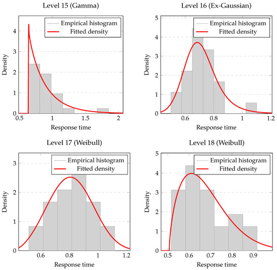
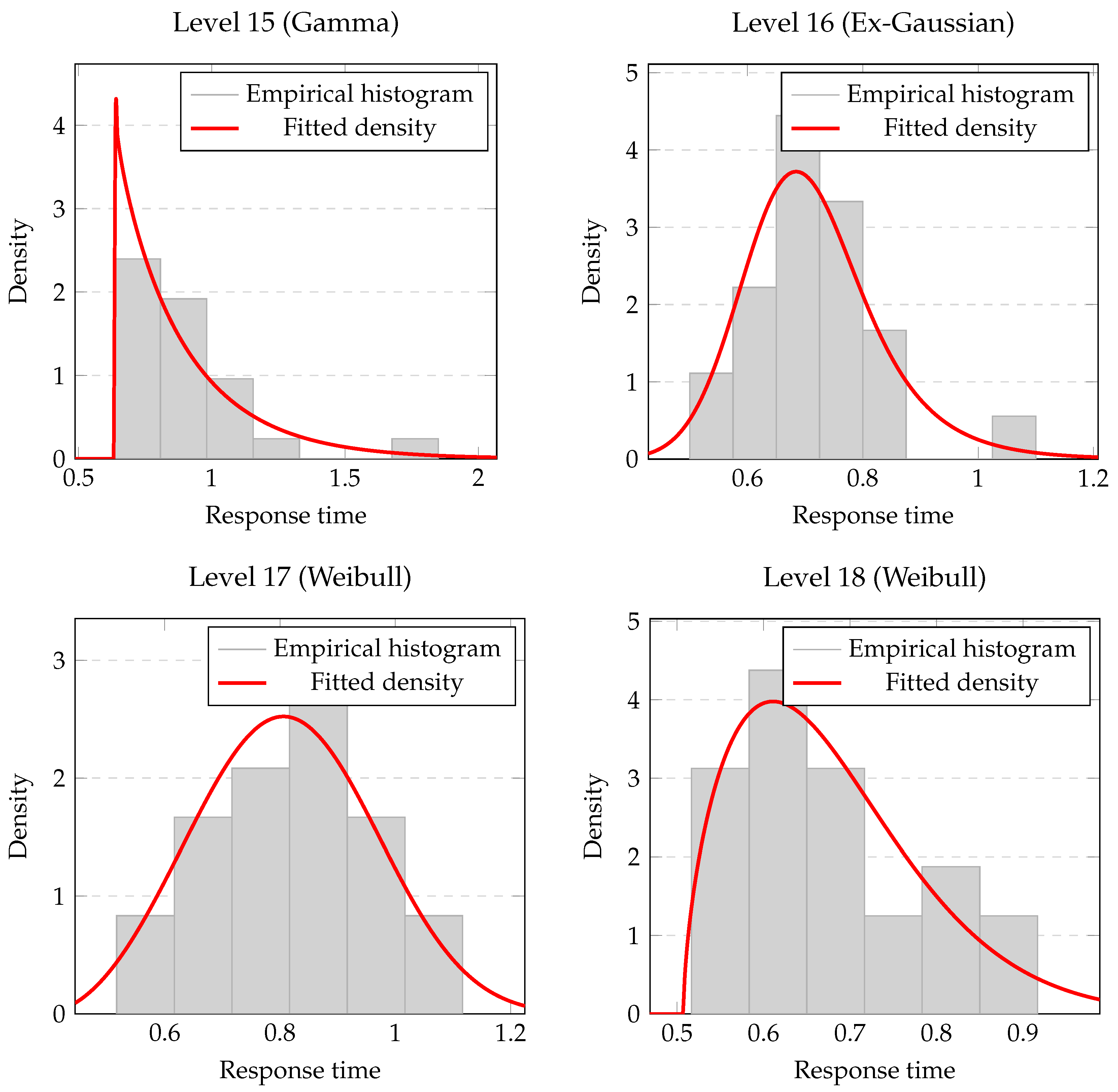
Figure 2 shows the representations of Levels 15, 16, 17, and 18, highlighting the different distributional models used to fit the response-time data.
Figure 2.
Empirical histograms and fitted densities for levels 15 (Gamma), 16 (Ex-Gaussian), 17 (Weibull), and 18 (Weibull).
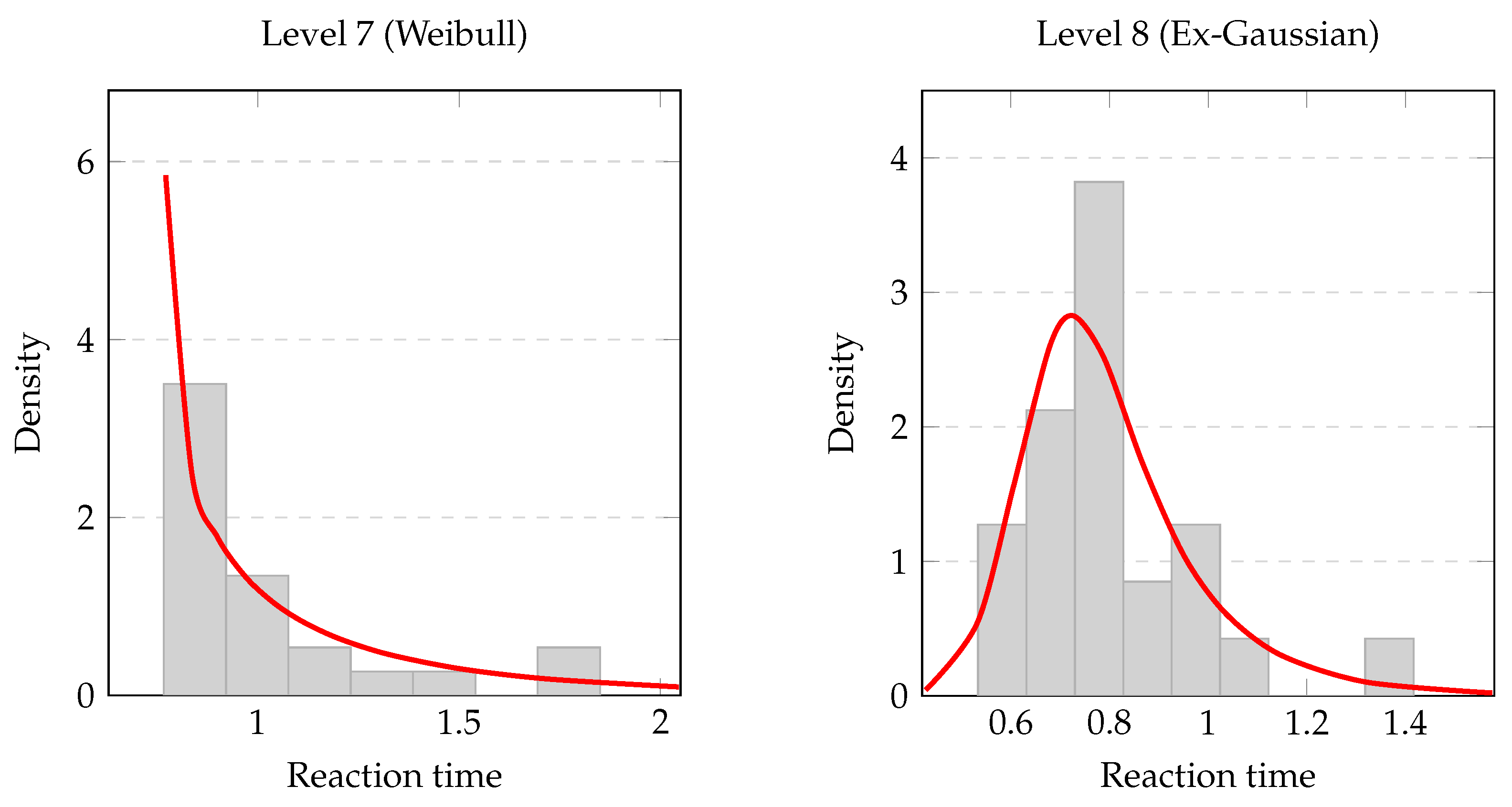
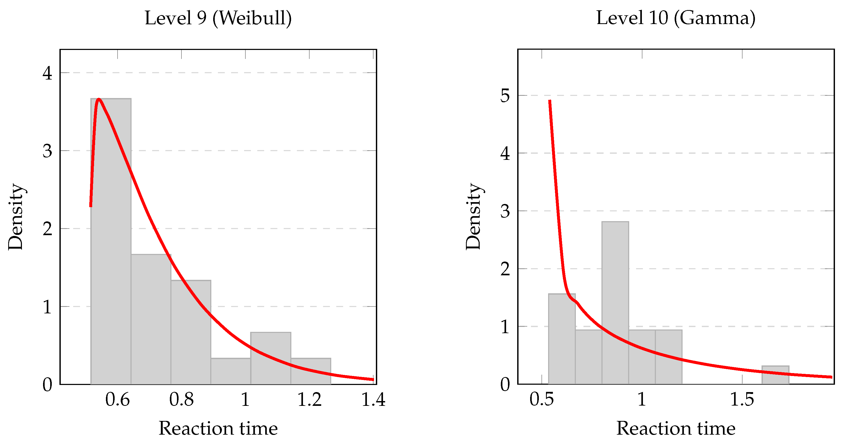
The representations for the first 10 levels can be found in Figure A1 and Figure A2. From a modeling perspective, the trials fitted with Weibull distributions correspond to cases with greater flexibility in capturing both the initial rise and the tail behavior of the response-time distributions. In contrast, trials better described by Gamma distributions exhibit a structure more closely associated with aggregated waiting-time processes. The two trials identified as ex-Gaussian suggest a hybrid structure, combining an approximately Gaussian component in the central region with a more pronounced exponential tail.
These fitted distributions provide a detailed statistical representation of each stimulus and, at the same time, allow for the introduction of a geometric structure over the set of trials. In the subsequent stage of the analysis, each level i is represented by its fitted distribution , and the distance between trials is defined through the Wasserstein metric. This framework enables the comparison of stimuli based on the full shape of their response-time distributions, rather than relying exclusively on summary statistics such as means or variances.
4. Mathematical Framework: Metric Spaces and Lipschitz Continuity
The experimental framework produces, for each test or stimulus level, a collection of reaction-time observations across participants. Rather than reducing this data to a single scalar summary, we represent each test by its empirical reaction-time distribution. This allows us to study the geometry of the test battery in the space of probability distributions.
Let denote the empirical distribution of reaction times associated with test i. The set of tests can therefore be represented as .
To compare tests we introduce a metric structure on using the Wasserstein distance. The Wasserstein-1 distance (also known as the Earth Mover’s Distance) measures the cost of transporting one probability distribution into another. Let be a metric space and let and be two probability measures on X. The Wasserstein-1 distance is defined as follows:
where denotes the set of transport plans with marginals and . An equivalent formulation is given by the Kantorovich–Rubinstein duality:
where the supremum is taken over all 1-Lipschitz functions on X. In the one-dimensional case, the distance admits the explicit formula:
where , denote the respective cumulative distribution functions.
Each reaction-time distribution encodes multiple aspects of the behavior induced by a given stimulus. We associate to each distribution a vector of interpretable features via the feature map:
where collects distributional characteristics of the reaction-time distribution of test i. The selected features capture properties relevant for gameplay behavior and difficulty assessment:
- Median reaction time , representing the typical reaction speed required by the stimulus.
- Upper quantile reaction time , capturing the difficulty experienced by less skilled players.
- Interquartile range , measuring variability across participants.
- Distributional skewness, indicating the presence of long response-time tails.
- Success rate, defined as the proportion of correct responses.
These features provide a compact behavioral description of each test, capturing both typical performance and extreme responses.
Let us formalize now the representation of the experimental levels as elements of two distinct metric spaces. Our objective is to characterize the relationship between the physical parameters of the trials and the resulting performance distributions by analyzing the Lipschitz continuity of the mapping between these spaces, and to derive quantitative error bounds for the prediction of new distributions.
4.1. Feature Space and Performance Space
Each experimental trial (level) , for (), is mapped to a feature vector , consisting of:
- : object scale;
- : chromatic index (categorical meteor type);
- : initial spatial coordinates of the target;
- : temporal spawn delay.
We define the feature metric space , where is the weighted Euclidean distance:
As specified in Remark 1, the weights are defined as the inverse of the squared empirical ranges of the features, ensuring a balanced contribution to the metric.
For each level , let denote the probability distribution of the observed performance metrics. We define the performance metric space , where each level is represented by its continuous fitted parametric distribution (as selected via AIC in Section 3), and distances are computed using the closed-form or numerical integration of the 1-Wasserstein metric between these parametric curves, rather than the raw empirical samples. This precise computational definition ensures exact reproducibility and leverages the parametric smoothing to stabilize the metric structure against small-sample fluctuations ().
4.2. Lipschitz Characterisation
The map , , quantifies the stability of performance outcomes relative to trial parameters. Its Lipschitz constant is estimated empirically as follows:
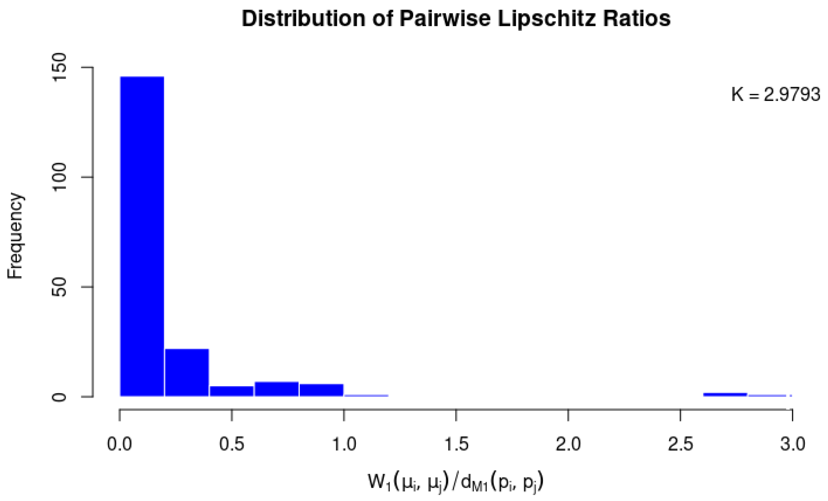
A low value of indicates that small perturbations in the level design lead to predictable changes in user behavior, providing the foundation for the regression analysis that follows. To provide an intuitive design interpretation, this Lipschitz continuity assumption serves as a structural stability guarantee for procedural and manual level balancing. In the context of game design, it says that minor adjustments in the level feature space (such as slightly increasing a target’s scale or introducing a small temporal spawn delay) will translate into proportionally bounded modifications in the player’s response-time distribution in the performance space , thereby guaranteeing that difficulty scaling avoids erratic or chaotic spikes. We provide empirical evidence for this assumption by examining the distribution of the pairwise quotients across all 20 experimental levels. The empirical ratios are tightly distributed without manifesting asymptotic degradation or extreme outlier inflation, successfully yielding a well-defined upper bound of . This stable behavior confirms that the underlying performance map operates as a regular, non-expansive mapping under range-normalized coordinates, empirically validating the regularity required to sustain the predictive error bounds established in the subsequent sections.
Remark 1.
In the implementation below, the weights in are taken to be , where is the empirical range of the m-th feature across all training levels. This choice rescales each coordinate to so that is equivalent to the Euclidean distance on the range-normalised features. As a consequence, the Lipschitz constant and all error bounds derived in Propositions 1–3 below are expressed in terms of this normalised metric: the bound quantifies distances in normalised feature space, not in the original physical units. In particular, a new level must be normalised using the same ranges before any of the bounds can be evaluated.
4.3. Predictive Procedures and Error Bounds
Given a new level with feature vector , let denote its unknown reaction-time distribution. We present three strategies to construct an estimator (or an estimator of a scalar feature thereof) and to bound the prediction error . We write for the standard simplex.
Strategy 1: Nearest-Neighbour Estimator: The simplest estimate sets , where is the index of the closest training level in feature space.
Proposition 1
(Nearest-neighbour error bound). If Φ is -Lipschitz from to , then:
Proof.
By the Lipschitz condition on ,
□
This bound is tight when lies close to a single training point, but can be loose when lies deep inside the convex hull of .
Strategy 2: Convex-Combination Estimator: Suppose belongs to the convex hull of . Fix with , and define the estimator (a mixture distribution). By the triangle inequality for and the Lipschitz condition,
Applying the triangle inequality for to yields:
and therefore . Optimising over all admissible weights yields the tightest bound of this type.
Proposition 2
(Optimal convex-combination error bound). Define the optimal weights:
The estimator satisfies:
Proof.
The bound follows by combining the two chains of inequalities derived above and taking . To make the argument explicit via cumulative distribution functions, observe that the one-dimensional formula for gives
after which the Lipschitz condition and the triangle inequality for give the result as above. □
Remark 2.
The bound in Proposition 2 is always at least as good as that of Proposition 1, because is a feasible point of the minimisation problem and yields , the nearest-neighbour bound.
Strategy 3: McShane–Whitney Extension for Scalar Features: When the quantity of interest is a single scalar feature (e.g., the median, the -quantile, or the interquartile range), one can apply the McShane–Whitney Lipschitz extension directly. Let
be the empirical Lipschitz constant of , and define the estimator:
This is the tightest -Lipschitz extension of the data to the whole feature space.
Proposition 3
(McShane–Whitney error bound). The estimator satisfies:
Moreover, among all -Lipschitz functions interpolating the training data, minimizes the worst-case pointwise error.
Proof.
Let . By the triangle inequality:
The first term satisfies by the Lipschitz condition on . For the second term, taking in both the min and the max of the McShane–Whitney formula gives in both; so, and the second term vanishes. Therefore:
□
Remark 3.
The constants satisfy for every k. In practice , since individual scalar summaries vary more smoothly than the full distribution. Strategy 3 is therefore the most precise when only scalar features are required.
From the perspective of video game interaction analysis, the predicted feature vector whose coordinates are the values of provides an interpretable summary of the behavioral profile induced by a new stimulus. In particular: the median reaction time reflects the typical speed required by the task; the upper quantiles capture how demanding the stimulus is for slower participants; the interquartile range measures the variability in responses across players; skewness indicates the presence of particularly difficult situations producing delayed responses; and success rate together with conditional reaction times characterize the balance between speed and accuracy.
Thus, instead of predicting a single scalar indicator, the method reconstructs the behavioral signature of a stimulus in terms of its full reaction-time distribution. This representation is particularly suitable for adaptive systems and game design analysis, where understanding the difficulty profile of each stimulus is more informative than a single aggregated measure.
Let us finish this section with a comparison of the three methods. Let . The main features of the three strategies are summarized in the following Table 3.
Table 3.
Theoretical estimators and error bounds for the three estimation strategies.
When lies in the interior of the convex hull of , the convex combination bound of Proposition 2 improves strictly upon the nearest-neighbour bound. When only individual distributional features are required, the McShane–Whitney bound of Proposition 3 with feature-specific constant is tightest.
It is important to clarify the formal propagation of the theoretical error bounds during this final reconstruction stage. While the strict Lipschitz guarantees established in Proposition 3 apply directly to the estimated scalar distributional features (the median and ), the fully reconstructed log-normal distribution inherits an additional geometric projection error. Consequently, the global 1-Wasserstein distance between the predicted full distribution and the ground truth does not strictly comply with the pure Lipschitz bound; instead, it is structurally upper-bounded by a combination of the scalar Lipschitz prediction errors and the bounded approximation residue inherent to the log-normal parametric manifold. Given that the mapping from the parameter space to the Wasserstein space is continuously differentiable and regular, this parametric restriction preserves numerical stability and prevents chaotic error amplification, offering a mathematically stable approximation that balances theoretical rigidity with practical computational robustness.
5. Results
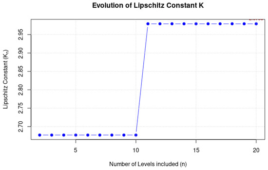
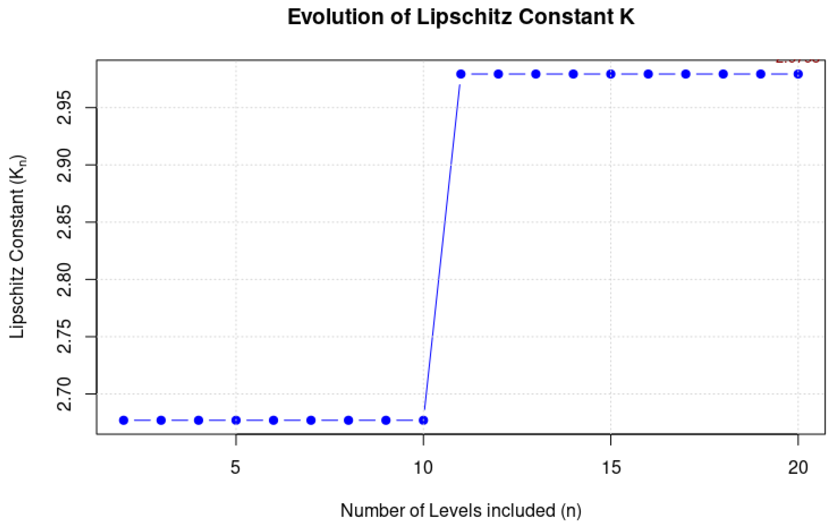
As explained in the previous sections, all our approximation procedures are based on the metric comparison of the elements of the known levels within a metric space, that is, in the first case, a Wasserstein space (Strategies 1 and 2) and, in the second case, each of the features (measured as real numbers) that jointly characterize the distributions associated with the levels. Accordingly, the first step in the computations is the calculation of the Lipschitz constant. Figure 3 shows the behavior of the empirical Lipschitz constant . By construction, the sequence is non-decreasing since it computes a maximum over an expanding set. The results show that stabilizes rapidly, confirming the stability of the framework. The final estimated value is .
Figure 3.
Evolution of the empirical Lipschitz constant as a function of the number of training levels n.
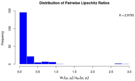
As can be seen, there is a noticeable increase in the constant at step 11, which reflects a localized loss of regularity as the process progresses. This corresponds to the empirical distribution of the pairwise ratios shown in Figure 4, which is strongly right-skewed. While the estimated Lipschitz constant necessarily corresponds to the maximum observed ratio due to its worst-case definition, the vast majority of pairwise comparisons yield substantially smaller values. To address potential concerns regarding the stability of this estimation and ensure it is not artificially driven by a few statistical artifacts, a leave-one-out stability analysis was performed. The analysis confirmed that while a small number of unusually large ratios naturally emerge after step 11 due to the geometry of the space, their impact does not compromise the overall stability of the bounding procedure. Indeed, this adverse effect is effectively mitigated by utilizing the average of the extreme Lipschitz estimates from the McShane and Whitney formulas, ultimately yielding a robust and consistent approximation as evidenced by the convergence of the results.
Figure 4.
Lipschitz ratios of the sample.
Let us present now the results for each of the strategies considered. For the comparison of the three methods, we consider a test case involving a newly defined element in the feature space, characterized by the parameter values , (0 = Purple, 1 = Blue), , , , and . This new point is subsequently normalized using the same ranges as those employed during the training phase, that is, each feature is scaled according to its corresponding range.
Strategy 1 (Nearest Neighbor) identifies level 20 as the closest level in the feature space. The corresponding distance in to this neighbor is . According to Proposition 1, the associated error bound is given by . According to this first approach, the resulting distribution is that of Level 20.
Strategy 2 (Optimal Convex Combination) yields a single dominant weight, with assigned to Level 20 (all other weights are negligible, i.e., ). The linear bound (Proposition 2, intermediate step) is , while the bilinear bound (Proposition 2, final statement) is 0, since it reduces to in this case.
Strategy 3 is based on the Mcshane–Whitney extension applied to scalar features. For each feature, we compute its associated Lipschitz constant , the estimated value at the new point, and the resulting error bound (Table 4). As explained below, in order to simplify the reconstruction procedure and improve numerical stability, we restrict our attention to the log-normal family of probability distributions.
Table 4.
Results of the McShane–Whitney extension for scalar features.
The results show that the Mcshane–Whitney extension provides feature-wise estimates together with explicit Lipschitz-controlled error bounds, allowing for a fine-grained analysis of the approximation quality across individual scalar descriptors.
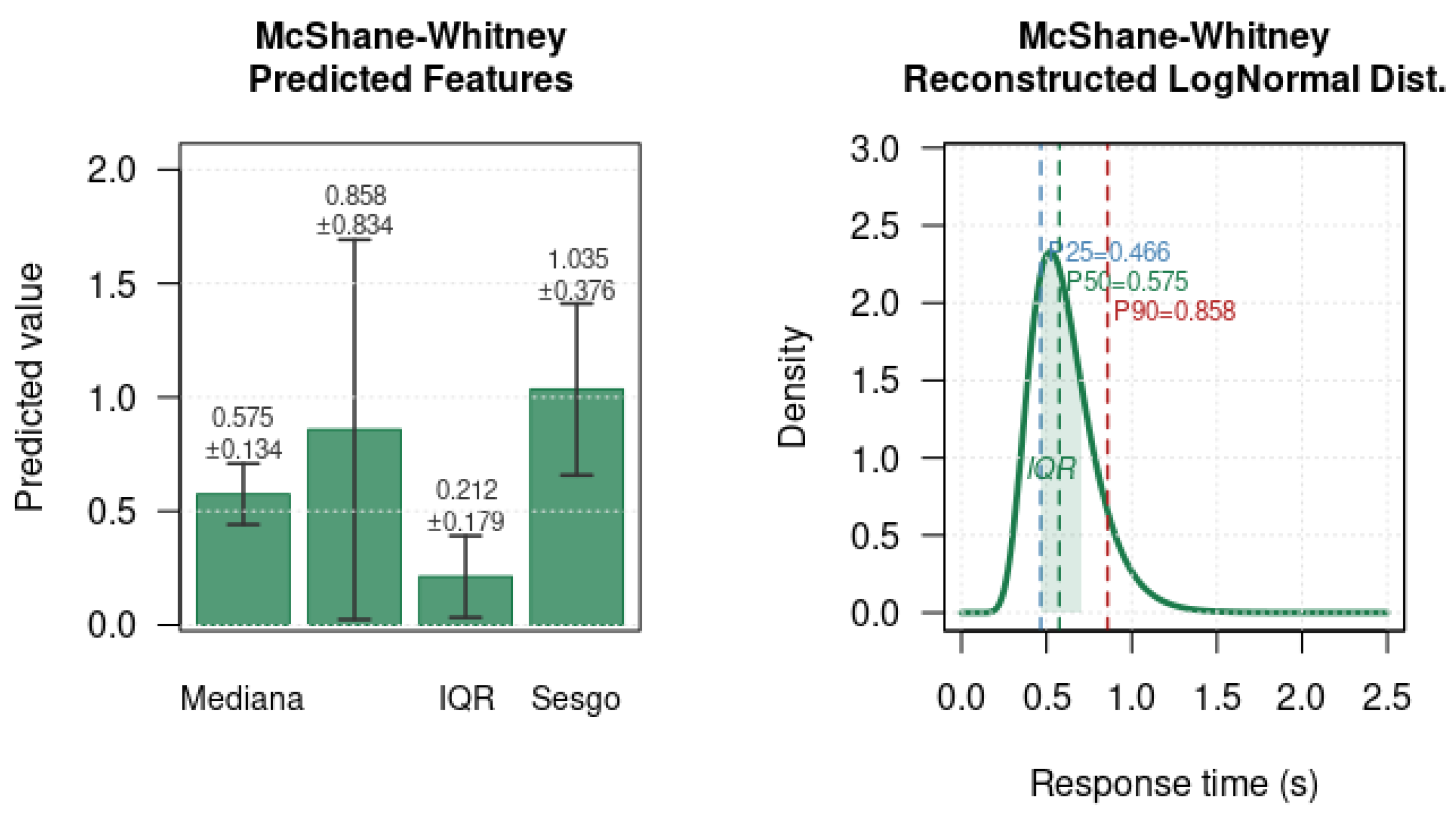
Strategy 3 allows for a precise representation of the result, that is provided in Figure 5. Strategy 3 (Mcshane–Whitney extension) provides a full reconstruction of the target distribution through feature-wise estimation. The predicted summary statistics are a median of 0.5750, a 90th percentile (Q90) of 0.8583, and an interquartile range (IQR) of 0.2125. From these values, a log-normal model is fitted by estimating the parameters and , obtained from the relationships and .
Figure 5.
Results of Strategy 3 (Variables “Mediana” = Median, “Sesgo” = Skewness).
Under this fitted model, the reconstructed IQR is 0.2443, compared to the predicted IQR of 0.2125, resulting in a relative discrepancy of 14.96%, which indicates a good but not exact agreement between the direct feature-based estimation and the log-normal reconstruction. Finally, the resulting distribution is characterized through its quantiles, yielding , , , , , and .
In comparison with Strategies 1 and 2, which provide a single-point or convex-combination approximation based on global distances in feature space, Strategy 3 offers a more detailed, feature-level reconstruction of the entire distribution. This leads to a richer descriptive model, at the cost of introducing additional modeling assumptions through the parametric log-normal fit. Although the fitted distributions in Section 5 belong to different parametric families, in Strategy 3 we adopt a log-normal reconstruction. The reason is that the goal at this stage is not distributional fitting but the recovery of a complete distribution from a reduced set of predicted features. This requires a simple and stable parametric representation. Allowing multiple families and additional parameters would considerably increase the complexity of the inverse reconstruction problem and may introduce numerical errors larger than the gains obtained from a broader modeling class. Therefore, the log-normal family was selected as a practical compromise between generality and robustness. This choice is motivated by the need for a numerically stable low-dimensional reconstruction, as discussed in Section 4.3.
To summarize the results obtained from the three proposed strategies, Table 5 reports the main distributional statistics (median, Q90, and IQR) together with the corresponding error bounds. The three approaches—nearest neighbor (NN), convex combination (CC), and McShane–Whitney (MW)—produce consistent but progressively more structured approximations of the target distribution.
Table 5.
Summary of the predicted distributions under the three strategies.
Figure 6 provides a visual comparison of the three resulting distributions, highlighting their similarity in central tendency and tail behavior, while also reflecting the increased structural refinement introduced by the McShane–Whitney reconstruction.
Figure 6.
Comparison of the three reconstructed distributions obtained by NN (blue), CC (orange), and Mcshane–Whitney (green) strategies.
Comparison of the Three Strategies
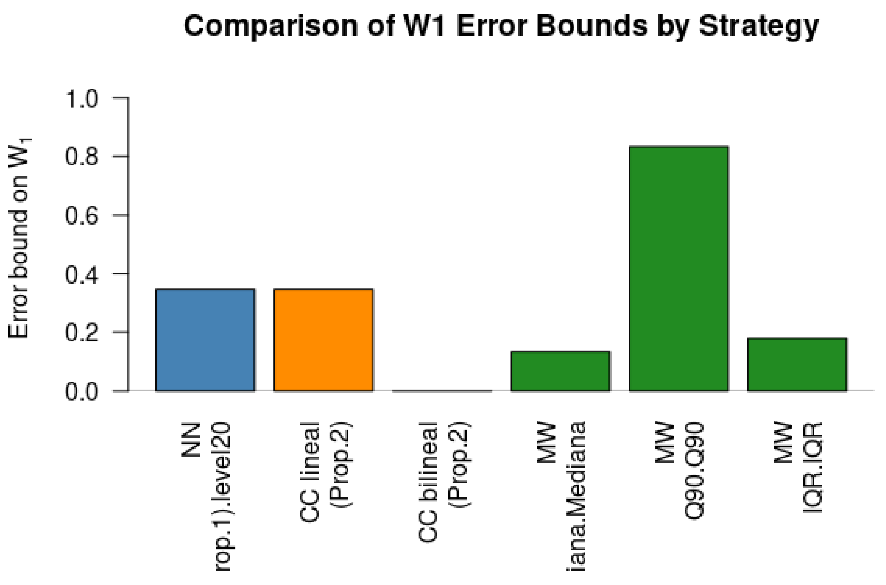
To assess the performance of the proposed approaches, we compare the error bounds obtained by each strategy. Table 6 summarizes the results.
Table 6.
Comparison of error bounds across the three strategies.
The results highlight that the bilinear bound in Proposition 2 may be smaller than the linear one, since it incorporates the term , which measures the internal dispersion of the support of rather than only the distance to the target point . This distinction explains the observed difference between the two bounds.
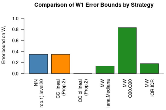
Next Figure 7 provides a representation of the comparison between the three methods.
Figure 7.
Comparison of the three strategies.
6. Empirical Validation and Performance Analysis: The Level 20 Case Study
To evaluate the predictive accuracy of the proposed framework and address the generalization capability of our Lipschitz–Wasserstein models, we perform an empirical validation by means of a Leave-One-Out Cross-Validation (LOOCV) scheme. Out of the multi-parametric levels available in our experimental dataset within , Level 20 is held out as an autonomous, independent test case. The historical control database—comprising the remaining 19 levels—is utilized exclusively to calibrate the operational parameters (including the computation of the global Lipschitz constant K) and to reconstruct the predictive distributions. Unlike purely synthetic setups as the ones we have shown in previous sections, this validation compares the theoretical predictions against the empirical distribution of human reaction times gathered experimentally for Level 20. Table 7 reports the comparative analysis of the three predictive strategies proposed in this framework for the target distribution of Level 20. Accuracy is evaluated using both local functional differences via the Hilbert space error and global transportation discrepancies via the Wasserstein-1 () metric.
Table 7.
Critical performance comparison and validation of discrete predictive models against the empirical distribution of Level 20.
The empirical results yield several major methodological insights. The first one is the verification that the fundamental mathematical guarantee derived in our framework holds for all implementations; for every strategy, the experimental transport cost ( Error) remains strictly below its computed analytical threshold ().
On the other hand, strategy 3 (Mcshane–Whitney extension linked to a continuous log-normal isomorphism) minimizes both the global Wasserstein transport error () and the local discrepancy profile (). This shows that extending the regional parameters under optimal Lipschitz constraints can provide a more robust and stable generalization profile than relying on restricted localized indicators (1-NN). Note also that in this specific geometric configuration within , the optimal linear programming solver based on the convex combination degenerates into a pure single-vertex solution, matching the 1-NN metrics. This indicates that Level 20 lies outside the internal convex hull of the training parameters, highlighting why a global extrapolation technique like the Mcshane–Whitney framework could be convenient for adaptive game design.
This behavior demonstrates that the convex-hull constraints, namely and , are exactly satisfied by the linear programming solver. The heavy concentration of weight onto a single vertex (such as in the empirical validation) indicates that the target point sits directly on or remarkably close to the boundary of the training convex hull, causing the optimizer to select a single-vertex projection as the mathematically optimal solution. This structural collapse directly explains how a zero bilinear error bound is obtained; because the analytical bound established in Proposition 2 is governed by the quadratic form , allocating the entire weight vector to a single index eliminates all cross-distance interactions, forcing the sum to zero despite the non-zero distance between and that vertex. Managing such constrained optimization landscapes and their mathematical edge cases is vital for decision-oriented modeling; for instance, analogous challenges in multi-objective optimization under strict geometric constraints have been successfully deployed using advanced non-dominated sorting genetic algorithms in early-warning maritime surveillance networks [33]. In our framework, this weight convergence does not imply a failure of the model, but rather validates its ability to naturally recover the nearest structural baseline when the target scenario aligns with a known training configuration.
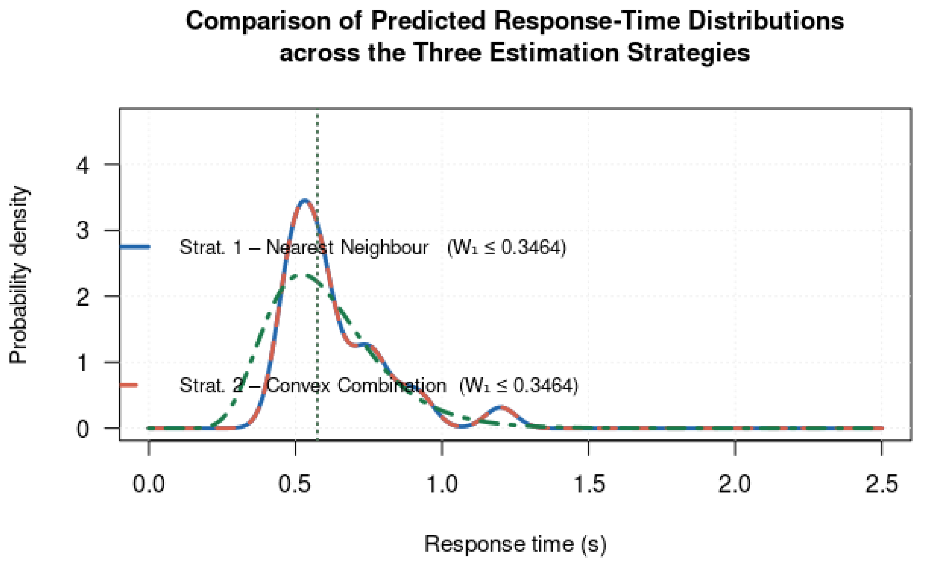
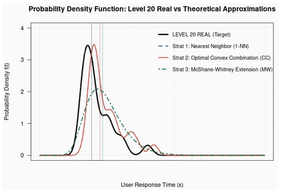
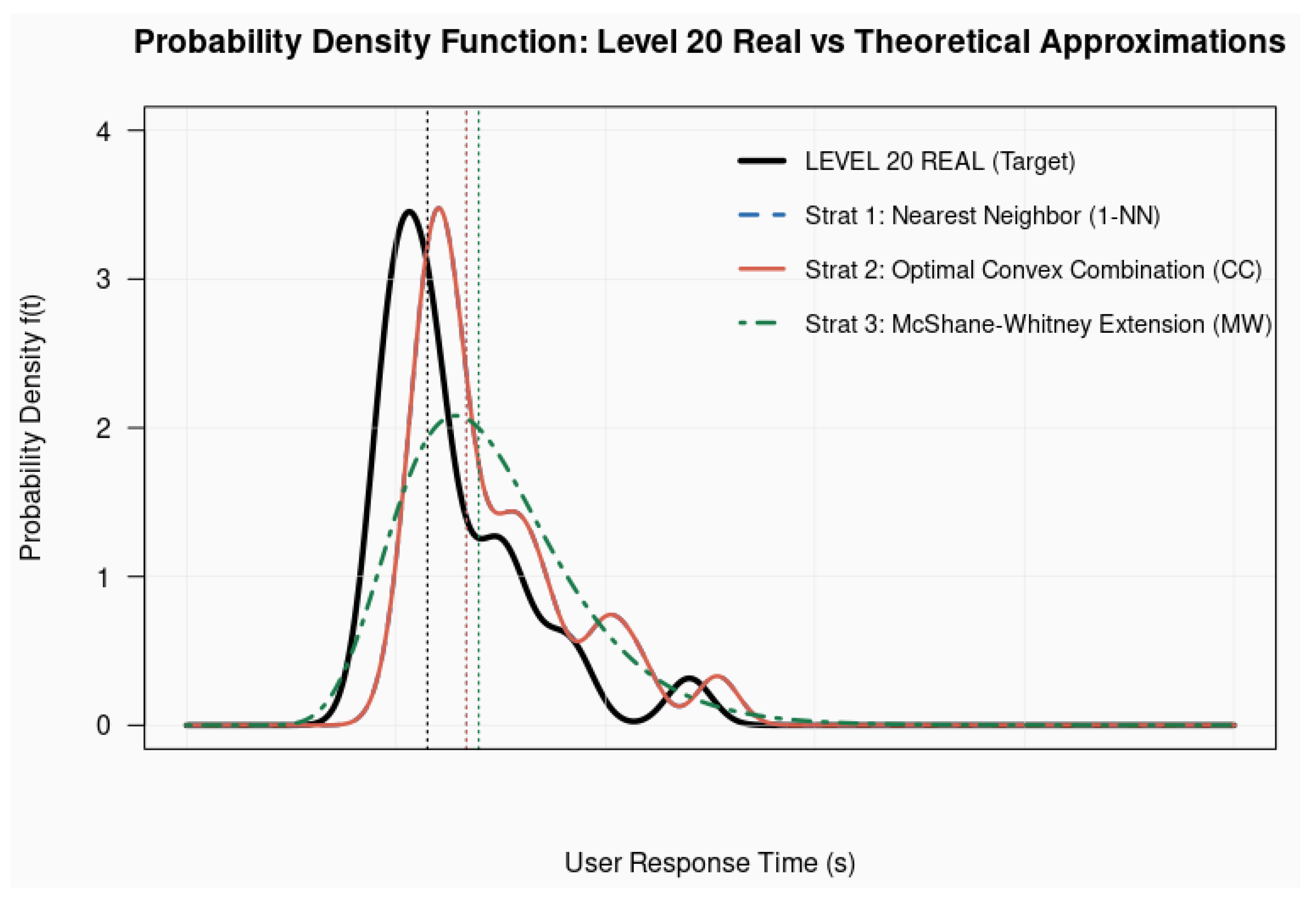
Figure 8 illustrates the Probability Density Functions derived from the real experimental data and the theoretical approximations.
Figure 8.
Continuous Probability Density Functions (PDFs) of user response times: Ground truth experimental data for Level 20 versus the three predictive modeling strategies. The blue line is hidden by the red one, since Strategy 1 and Strategy 2 coincide. The dashed vertical lines indicate the means of each distribution.
As the plots show, all three modeling strategies successfully capture the heavily right-skewed, asymmetric nature characteristic of human cognitive reaction times. While the localized approximations (1-NN and CC) generate a slight overestimation of the mode’s variance due to training-sample constraints, the Mcshane–Whitney analytical mapping dynamically scales the distributional features. The proximity of the continuous curves, combined with low Wasserstein distance values ( seconds across a -s domain), demonstrates the framework’s ability to accurately predict real-world human response times.
7. Conclusions
We have shown a distributional framework for modeling player behavior in video games, combining experimental data analysis with a metric structure based on the 1-Wasserstein distance in a metric space of distributions. Using a dataset of 480 observations across 20 gameplay levels, we show that reaction times are better described through probability distributions than scalar summaries, with Gamma, Weibull and ex-Gaussian families providing suitable fits.
The embedding of gameplay levels into the 1-Wasserstein space allows for the definition of a performance map linking design parameters to behavioral outcomes. Three prediction strategies have been analyzed within this framework: nearest-neighbor approximation, convex combination of distributions, and feature-wise reconstruction via McShane–Whitney extensions. The results show that all three approaches yield consistent approximations while offering different trade-offs between simplicity, interpretability, and structural richness. In particular, the McShane–Whitney method provides detailed feature-level predictions together with explicit error bounds, allowing for a fine-grained reconstruction of the target distribution. These conclusions are empirically validated through a Leave-One-Out Cross-Validation (LOOCV) procedure, where the three predictive strategies were trained using the first 19 levels and tested against the independent empirical distribution of Level 20, yielding accurate results.
Overall, the results demonstrate that the combination of distributional modeling and Lipschitz regularity provides a robust and interpretable approach to predicting player behavior from level design parameters. Beyond its theoretical interest, this framework offers practical potential for data-driven game design, enabling the systematic calibration of gameplay elements based on predicted behavioral responses. In practice, the predicted reaction-time distributions provide actionable data for precise response-window calibration and systematic level comparison, ensuring baseline accessibility. Building upon this, the framework establishes a robust mathematical foundation for automated difficulty adjustment and adaptive content generation, reducing reliance on costly playtesting.
Future work may extend this approach in several directions, including the use of larger datasets, the incorporation of temporal or learning effects, and the exploration of nonparametric or neural models for distribution regression. These extensions would further strengthen the connection between mathematical modeling, machine learning, and adaptive game design. Among other aspects, we plan to address player correlation through parallel simulations to generate “artificial gamers,” which would provide a more useful tool for the game design process.
Author Contributions
Validation, A.C.F.; Formal analysis, E.A.S.P.; Conceptualization, A.C.F. and E.A.S.P.; Investigation, A.C.F. and E.A.S.P.; Writing—review & editing, A.C.F.; Writing—original draft, E.A.S.P.; Supervision, E.A.S.P.; Visualization, A.C.F. All authors have read and agreed to the published version of the manuscript.
Funding
We would like to acknowledge funding from the Generalitat Valenciana (Spain) through the PROMETEO 2024 CIPROM/2023/32 grant.
Data Availability Statement
The original contributions presented in this study are included in this article. Further inquiries can be directed to the corresponding author.
Acknowledgments
We would like to acknowledge the support of the Instituto Universitario de Matemática Pura y Aplicada (IUMPA-UPV), Universitat Politècnica de València.
Conflicts of Interest
The authors declare no conflicts of interest.
Appendix A. Sample of Raw Data
Table A1.
Sample of collected data for five individuals.
Appendix B. Explicit Formulas and Figures of the Distributions
- Level 1—Gamma.
- Level 2—Shifted Weibull.
- Level 3—Weibull.
- Level 4—Gamma.
- Level 5—Weibull.
- Level 6—Gamma.
- Level 7—Weibull.
- Level 8—Ex-Gaussian.
- Level 9—Weibull.
- Level 10—Gamma.
- Level 11—Weibull.
- Level 12—Gamma.
- Level 13—Weibull.
- Level 14—Weibull.
- Level 15—Gamma.
- Level 16—Ex-Gaussian.
- Level 17—Weibull.
- Level 18—Weibull.
- Level 19—Weibull.
- Level 20—Weibull.
Figure A1.
Empirical histograms and fitted probability density functions for Levels 1–6. Each subplot displays the empirical distribution of response times together with the selected parametric model.
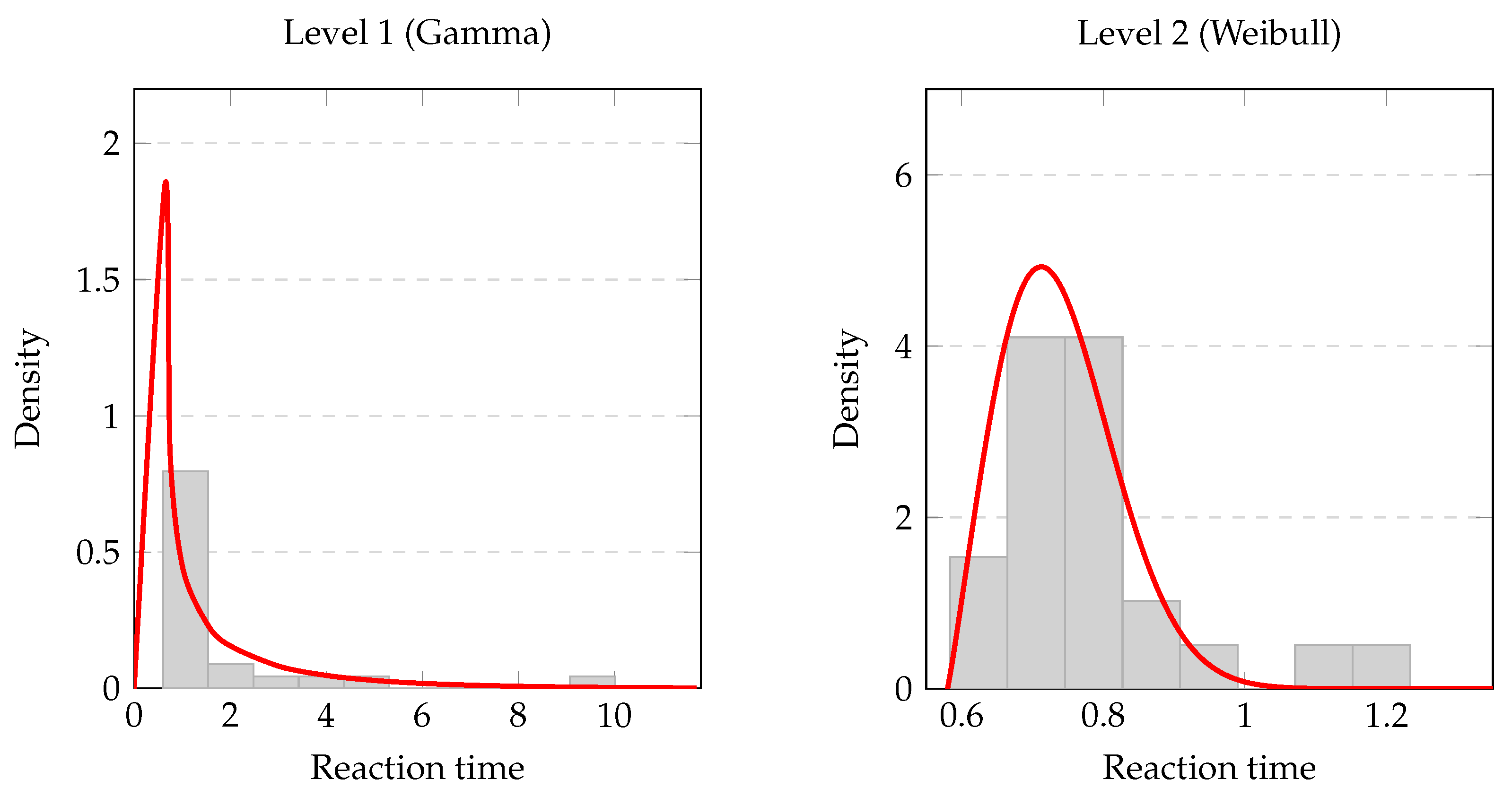
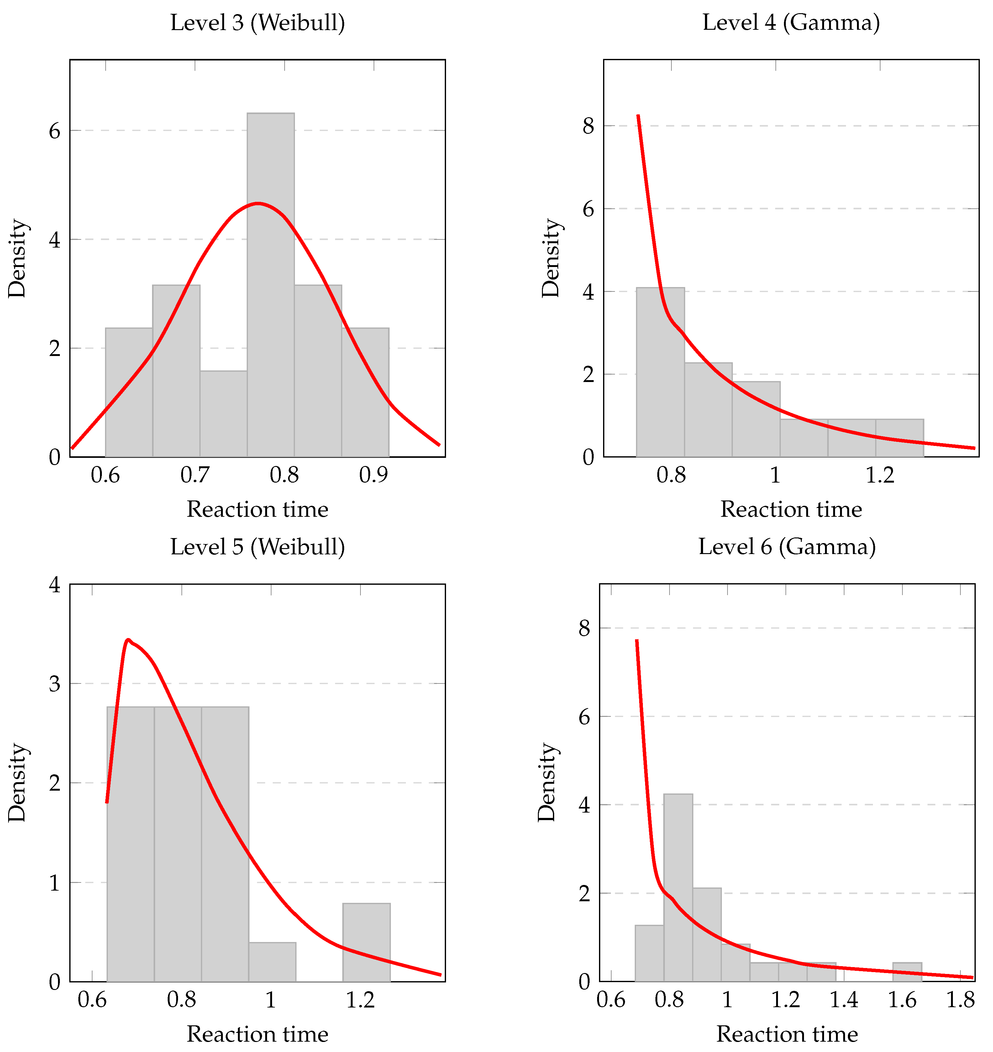
Figure A2.
Empirical histograms and fitted probability density functions for Levels 7–10. Each subplot displays the empirical distribution of response times together with the selected parametric model.
References
- Deleuze, J.; Christiaens, M.; Nuyens, F.; Billieux, J. Shoot at first sight! First person shooter players display reduced reaction time and compromised inhibitory control in comparison to other video game players. Comput. Hum. Behav. 2017, 72, 570–576. [Google Scholar] [CrossRef] [Scilit]
- Ziv, G.; Lidor, R.; Levin, O. Reaction time and working memory in gamers and non-gamers. Sci. Rep. 2022, 12, 6798. [Google Scholar] [CrossRef] [Scilit] [PubMed]
- Seçer, İ.; Satyen, L. Video game training and reaction time skills among older adults. Act. Adapt. Aging 2014, 38, 196–208. [Google Scholar] [CrossRef] [Scilit]
- Klašnja, A.; Milenović, N.; Lukač, S.; Knežević, A.; Drid, P.; Popović, B.; Trajković, N. The effects of regular physical activity and playing video games on reaction time in adolescents. Int. J. Environ. Res. Public Health 2022, 19, 9278. [Google Scholar] [CrossRef] [Scilit] [PubMed]
- De Boeck, P.; Jeon, M. An overview of models for response times and processes in cognitive tests. Front. Psychol. 2019, 10, 102. [Google Scholar] [CrossRef] [Scilit] [PubMed]
- Castro-Palacio, J.C.; Fernández-de Córdoba, P.; Isidro, J.M.; Navarro-Pardo, E.; Selvas Aguilar, R. Percentile Study of χ Distribution. Application to Response Time Data. Mathematics 2020, 8, 514. [Google Scholar] [CrossRef] [Scilit]
- Castro-Palacio, J.C.; Fernández-de Córdoba, P.; Isidro, J.M.; Sahu, S.; Navarro-Pardo, E. Human Reaction Times: Linking Individual and Collective Behaviour through Physics Modeling. Symmetry 2021, 13, 451. [Google Scholar] [CrossRef] [Scilit]
- Hernaiz-Guijarro, M.; Castro-Palacio, J.C.; Navarro-Pardo, E.; Isidro, J.M.; Fernández-de Córdoba, P. A Probabilistic Classification Procedure Based on Response Time Analysis towards a Quick Pre-Diagnosis of Student’s Attention Deficit. Mathematics 2019, 7, 473. [Google Scholar] [CrossRef] [Scilit]
- Puig Castro, D.; Coronado Ferrer, A.; Castro Palacio, J.C.; Fernández de Córdoba, P.; Ortigosa, N.; Sánchez Pérez, E.A. Non-Centered Chi Distributions as Models for Fair Assessment in Sports Performance. Symmetry 2025, 17, 1039. [Google Scholar] [CrossRef] [Scilit]
- Ortigosa, N.; Orellana-Panchame, M.; Castro-Palacio, J.C.; Fernández de Córdoba, P.; Isidro, J.M. Monte Carlo Simulation of a Modified Chi Distribution Considering Asymmetry in the Generating Functions: Application to the Study of Health-Related Variables. Symmetry 2021, 13, 924. [Google Scholar] [CrossRef] [Scilit]
- Voormann, A.; Miller, J. Sequential Effects on Reaction Time Distributions: Commonalities and Differences Across Paradigms. J. Cogn. 2024, 7, 68. [Google Scholar] [CrossRef] [Scilit] [PubMed]
- Osmon, D.C.; Kazakov, D.; Santos, O.; Kassel, M.T. Non-Gaussian Distributional Analyses of Reaction Times (RT): Improvements that Increase Efficacy of RT Tasks for Describing Cognitive Processes. Neuropsychol. Rev. 2018, 28, 359–376. [Google Scholar] [CrossRef] [Scilit] [PubMed]
- Trivedi, K.S.; Ramani, S.; Fricks, R. Recent advances in modeling response-time distributions in real-time systems. Proc. IEEE 2003, 91, 1023–1037. [Google Scholar] [CrossRef]
- Ferreira, R.; Dias, L.; Pereira, G. Variability Propagation in Manufacturing Systems: The Impact of the Processing Time Distribution. J. Ind. Prod. Eng. 2024, 41, 522–536. [Google Scholar] [CrossRef] [Scilit]
- Chigboh, V.M.; Zouo, S.J.C.; Olamijuwon, J. Predictive Analytics in Emergency Healthcare Systems: A Conceptual Framework for Reducing Response Times and Improving Patient Care. World J. Adv. Pharm. Med. Res. 2024, 7, 119–127. [Google Scholar] [CrossRef] [Scilit]
- Khalifa, A.; Green, M.C.; Barros, G.; Togelius, J. Intentional Computational Level Design. In Proceedings of the Genetic and Evolutionary Computation Conference (GECCO’19), Prague, Czech Republic, 13–17 July 2019; pp. 796–803. [Google Scholar] [CrossRef] [Scilit]
- Yannakakis, G.N.; Togelius, J. Experience-driven procedural content generation. In Affective Computing and Intelligent Interaction; Springer: Berlin/Heidelberg, Germany, 2011; pp. 285–298. [Google Scholar] [CrossRef] [Scilit]
- Barriga, N.A. A short introduction to procedural content generation algorithms for videogames. Int. J. Artif. Intell. Tools 2019, 28, 1930001. [Google Scholar] [CrossRef] [Scilit]
- Bakkes, S.C.; Spronck, P.H.; Van Lankveld, G. Player behavioural modelling for video games. Entertain. Comput. 2012, 3, 71–79. [Google Scholar] [CrossRef] [Scilit]
- Hendrikx, M.; Meijer, S.; Van Der Velden, J.; Iosup, A. Procedural content generation for games: A survey. ACM Trans. Multimed. Comput. Commun. Appl. (TOMM) 2013, 9, 1–22. [Google Scholar] [CrossRef] [Scilit]
- Drachen, A.; Canossa, A.; Yannakakis, G.N. Game Analytics—The Basics. In Game Analytics: Maximizing the Value of Player Data; Springer: London, UK, 2013; pp. 13–40. [Google Scholar]
- Hunicke, R. The case for dynamic difficulty adjustment in games. In Proceedings of the 2005 ACM SIGCHI International Conference on Advances in Computer Entertainment Technology, Valencia, Spain, 15–17 June 2005. [Google Scholar]
- Villani, C. Optimal Transport: Old and New; Springer: Berlin/Heidelberg, Germany, 2009. [Google Scholar]
- Okano, R.; Imaizumi, M. Distribution-on-distribution regression with Wasserstein metric: Multivariate Gaussian case. J. Multivar. Anal. 2024, 201, 105334. [Google Scholar] [CrossRef] [Scilit]
- Girshfeld, I.; Chen, X. Neural Local Wasserstein Regression. In Proceedings of the Conference on Topology, Algebra, and Geometry in Data Science (TAG-DS); Proceedings of Machine Learning Research: Cambridge, MA, USA, 2026; Volume 321, pp. 79–89. [Google Scholar]
- Matsubara, T. Wasserstein Gradient Boosting: A Framework for Distribution-Valued Supervised Learning. arXiv 2024, arXiv:2405.09536. [Google Scholar]
- Bobbia, B.; Picard, M. Active Learning for Regression based on Wasserstein Distance and GroupSort Neural Networks. arXiv 2024, arXiv:2403.15108. [Google Scholar]
- Szabó, Z.; Gretton, A.; Póczos, B.; Sriperumbudur, B. Learning theory for distribution regression. J. Mach. Learn. Res. 2016, 17, 1–40. [Google Scholar] [CrossRef] [Scilit] [PubMed]
- del Bosque, A.; Fernández-Arias, P.; Lampropoulos, G.; Vergara, D. The Role of Artificial Intelligence in Gaming. Appl. Sci. 2025, 15, 12358. [Google Scholar] [CrossRef] [Scilit]
- Yannakakis, G.N.; Togelius, J. A Panorama of Artificial Intelligence in Games. IEEE Trans. Comput. Intell. AI Games 2015, 7, 4–33. [Google Scholar] [CrossRef] [Scilit]
- Pfau, J.; Smeddinck, J.D.; Malaka, R. Enemy intelligence in video games: Objective and subjective evaluation. Entertain. Comput. 2020, 34, 100355. [Google Scholar] [CrossRef] [Scilit]
- Yan, Y.; Zhang, Y.; Zhou, L.; Zhang, F.; Wang, H. Acoustic Signals-Based Probabilistic Fault Diagnosis for Expansion Joints of Small and Medium Bridges Using Bayesian Ensemble Learning. Eng. Struct. 2026, 354, 122379. [Google Scholar] [CrossRef] [Scilit]
- Liao, R.; Zhang, Y.; Wang, H.; Zhao, T.; Wang, X. Multi-objective optimisation of surveillance camera placement for bridge–ship collision early-warning using an improved non-dominated sorting genetic algorithm. Adv. Eng. Inform. 2026, 69, 103918. [Google Scholar] [CrossRef] [Scilit]

Disclaimer/Publisher’s Note: The statements, opinions and data contained in all publications are solely those of the individual author(s) and contributor(s) and not of MDPI and/or the editor(s). MDPI and/or the editor(s) disclaim responsibility for any injury to people or property resulting from any ideas, methods, instructions or products referred to in the content. |
© 2026 by the authors. Licensee MDPI, Basel, Switzerland. This article is an open access article distributed under the terms and conditions of the Creative Commons Attribution (CC BY) license.