Quantile Reparameterized Regression Model and Machine Learning with Long-Term Survivors

Abstract

We propose a quantile-based survival model that accounts for a cure fraction. By modeling unobserved event causes with a negative binomial distribution and time-to-event with the generalized log-logistic Weibull distribution, we estimate parameters using a frequentist framework. We validated our model and applied it to prostate cancer data to prove its practical use. Comparing it to a Random Survival Forest model, we highlight how different approaches handle long-term survival, ultimately weighing the balance between flexibility, interpretability, and predictive performance.

1. Introduction

Traditional survival models typically assume every individual in a population remains susceptible to the event of interest over the follow-up period, making it straightforward to evaluate how covariates influence recurrence times. However, in many scenarios, a subset of the population is genuinely cured of the risk. Conventional methods fail in these situations, producing heavily right-censored datasets that obscure the distinction between cured individuals and those simply not yet experiencing the event. Traditionally, this type of analysis uses the Cox mixture cure model to incorporate covariates into the cure proportion. However, because this approach relies on the proportional hazards assumption—which may not always hold—alternative cure fraction regression models should be explored.

In these long-term models, the exact number of event triggers is an unobservable random variable governed by a discrete probability distribution. Furthermore, the academic literature show numerous applications of cure fraction survival models that utilize Weibull, log-logistic, generalized gamma, and inverse Gaussian distributions (de Castro et al., 2010 [1]; Ortega et al., 2015 [2]; Yiqi et al., 2020 [3]). These models are applied to various cancers, including breast, prostate, leukemia, and melanoma.

Quantile regression for censored data provides a strong alternative to the Cox model when analyzing survival or duration data. Instead of estimating the average outcome, it models conditional quantiles based on covariates. This approach reveals how the impact of predictors varies across different points in the event-time distribution, yielding deeper insights into data variability.

Quantile regression models can also be useful in analyzing heteroscedastic data or in studying inhomogeneous populations, in addition to being robust to the presence of outliers. Some research related to this topic can be found in Wu and Yin (2013) [4], Peng (2021) [5], Wu and Yin (2017) [6], and Rodrigues et al. (2025) [7], among others, but these studies focus on quantile regression and cure fraction in mixture and defective models.

Assuming the number of competing causes for an event follows a negative binomial distribution, we construct a time-to-event quantile regression model based on the generalized odd log-logistic Weibull (GOLLW) distribution. Additionally, we evaluate random survival forests. Although this machine learning technique lacks an explicit cure rate model—making interpretation difficult when cured patients are present—it excels at capturing highly complex, assumption-free relationships between variables.

We compare the survival curves estimated by a cure rate model with those generated by a random forest. The objective is to analyze how each method assesses risk over time and identifies potential cured populations, highlighting their respective strengths and limitations. Additionally, we assess predictive performance using standard metrics to verify whether the flexibility of the machine learning approach yields greater accuracy in individual survival predictions.

This paper is organized as follows. Section 2 introduces the GOLLW quantile (GOLLWQ) model with a cure fraction. Section 3 presents the GOLLWQ regression model for the cure proportion and estimates its parameters using maximum likelihood. Section 4 compares the predictive performance of this new regression model with a machine learning approach based on random survival forests. Simulation studies are reported in Section 5, and Section 6 illustrates the utility of our proposed models through an analysis of a prostate cancer data set. Finally, Section 7 offers some concluding remarks.

2. A New Distribution for Long-Term Survivors

The GOLL-G family (Cordeiro et al., 2017 [8]) is a powerful tool for modeling data with complex behaviors and tail shapes by adding two parameters to an arbitrary parent distribution G. The GOLLW distribution is formed by taking the Weibull cumulative distribution function (cdf) as the baseline G

$$G(t;\rho )=1-exp\left[-{\left({\displaystyle \frac{t}{\gamma }}\right)}^{\sigma }\right],$$

(1)

where $\rho ={(\gamma ,\sigma )}^{\top }$, $\gamma >0$ is a scale, and $\sigma >0$ is a shape.

The cdf of the random variable $T\sim \mathrm{GOLLW}(a,b,\gamma ,\sigma )$ follows from Cordeiro et al. (2017) [8] as

$$F\left(t\right)=F(t;a,b,\rho )={\displaystyle \frac{{\left\{1-exp[-{\left(\frac{t}{\gamma }\right)}^{\sigma }]\right\}}^{ab}}{{\left\{1-exp[-{\left(\frac{t}{\gamma }\right)}^{\sigma }]\right\}}^{ab}+{\left[1-{\left\{1-exp[-{\left(\frac{t}{\gamma }\right)}^{\sigma }]\right\}}^b\right]}^a}}.$$

(2)

The quantile function (qf) of T is obtained by inverting (2):

$$\begin{array}{c}\hfill Q\left(q\right)=\gamma {\left\{-\log \left[1-{\left\{{\displaystyle \frac{q^{1/a}}{{(1-q)}^{1/a}+q^{1/a}}}\right\}}^{1/b}\right]\right\}}^{1/\sigma }.\end{array}$$

(3)

The parameter $\gamma$ for a reparameterized cdf of T in terms of its $\tau$th quantile is

$$\gamma =\mu {\left\{-\log \left[1-{\left\{{\displaystyle \frac{{\tau }^{1/a}}{{(1-\tau )}^{1/a}+{\tau }^{1/a}}}\right\}}^{1/b}\right]\right\}}^{-1/\sigma },$$

(4)

where $\mu >0$ is a location and $\tau \in (0,1)$ is the known quantile of T.

By inserting (4) in Equation (2), we obtain

$$F\left(t\right)={\displaystyle \frac{{\kappa }^{ab}\left(t\right)}{{\kappa }^{ab}\left(t\right)+{\left[1-{\kappa }^b\left(t\right)\right]}^a}},$$

(5)

where

$$\begin{array}{c}\hfill \kappa \left(t\right)=1-exp\left[-w(a,b,\tau ){\left({\displaystyle \frac{t}{\mu }}\right)}^{\sigma }\right]\end{array}$$

(6)

$$\begin{array}{c}\hfill \mathrm{and}w(a,b,\tau )=-\log \left\{1-{\left[{\displaystyle \frac{{\tau }^{1/a}}{{(1-\tau )}^{1/a}+{\tau }^{1/a}}}\right]}^{1/b}\right\}.\end{array}$$

(7)

The reparameterized pdf of T is determined by a simple differentiation of $F\left(t\right)$

$$\begin{array}{c}\hfill f\left(t\right)={\displaystyle \frac{ab\sigma w(a,b,\tau )t^{\sigma -1}[1-\kappa \left(t\right)]{\kappa }^{ab-1}\left(t\right){\left[1-{\kappa }^b\left(t\right)\right]}^{a-1}}{{\mu }^{\sigma }{\left\{{\kappa }^{ab}\left(t\right)+{\left[1-{\kappa }^b\left(t\right)\right]}^a\right\}}^2}}.\end{array}$$

(8)

Equation (8) is called the GOLLW quantile (GOLLWQ) distribution. Henceforth, we denote $T\sim GOLLWQ(a,b,\mu ,\sigma |\tau )$ for a fixed and prespecified quantile level $\tau \in (0,1)$, with pdf given by (8). For a fixed quantile level $\tau \in (0,1)$, the parameter $\mu$ represents the $\tau$th quantile of T. Therefore, $\tau$ is not treated as an unknown model parameter and is not estimated jointly with $\mu$. Instead, each fixed value of $\tau$ defines a distinct quantile-parameterized model, with $\mu$ acting as the corresponding location parameter.

The qf of T is obtained by replacing (4) with (3):

$$t=Q\left(q\right)=\mu {\left\{{\displaystyle \frac{\log \left\{1-{\left[\frac{q^{1/a}}{{(1-q)}^{1/a}+q^{1/a}}\right]}^{1/b}\right\}}{\log \left\{1-{\left[\frac{{\tau }^{1/a}}{{(1-\tau )}^{1/a}+{\tau }^{1/a}}\right]}^{1/b}\right\}}}\right\}}^{1/\sigma },0<q<1.$$

(9)

Let the unobservable number of causes for the event of interest be denoted as M. While M is typically modeled by a Poisson distribution in long-term survival studies, we instead assume it follows a negative binomial (NB) distribution with parameters $\theta$ and $\eta$, and the probability mass function (pmf) (de Castro et al., 2010 [1])

$$P(M=m;\theta ,\eta )={\displaystyle \frac{\Gamma ({\eta }^{-1}+m)}{\Gamma \left({\eta }^{-1}\right)m!}}{\left({\displaystyle \frac{\eta \theta }{1+\eta \theta }}\right)}^m{(1+\eta \theta )}^{-1/\eta },m=0,1,2,\dots ,$$

(10)

where $\theta >0$, $\eta \ge -1$ and $\eta \theta +1>0$. Negative values of $-1\le \eta <0$ imply m from 0 to the largest integer less than ${\eta }^{-1}$. We have $E\left(M\right)=\theta$ and $Var\left(M\right)=\theta +\eta {\theta }^2$. Thus, overdispersion occurs if $\eta >0$ and underdispersion if $\eta <0$.

We assume, conditional on M, that the random variables (rvs) $T_i$’s are independent and identically distributed (iid) with cdf $F\left(t\right)$ representing the time to the event of interest due to unknown causes. These rvs and M are considered independent. The observable time to the current event is defined by $X=\min \{T_1,\cdots ,T_M\}$. In this framework, the survival function for the entire population is (Tsodikov et al., 2003 [9])

$$\begin{array}{c}\hfill S_{\mathrm{pop}}\left(t\right)={[1+\eta \theta F\left(t\right)]}^{-1/\eta },\end{array}$$

(11)

and the cured fraction is $p_0={(1+\eta \theta )}^{-1/\eta }$.

The negative binomial GOLLWQ (NBGOLLWQ) model with long-term survivors is obtained by inserting (5) in Equation (11):

$$S_{\mathrm{pop}}\left(t\right)={\left\{1+{\displaystyle \frac{\eta \theta {\kappa }^{ab}\left(t\right)}{{\kappa }^{ab}\left(t\right)+{\left[1-{\kappa }^b\left(t\right)\right]}^a}}\right\}}^{-{\displaystyle \frac{1}{\eta }}}.$$

(12)

The corresponding population density function is

$$\begin{array}{ccc}\hfill f_{\mathrm{pop}}\left(t\right)& =& {\displaystyle \frac{\theta ab\sigma w(a,b,\tau )t^{\sigma -1}[1-\kappa \left(t\right)]{\kappa }^{ab-1}\left(t\right){\left[1-{\kappa }^b\left(t\right)\right]}^{a-1}}{{\mu }^{\sigma }{\left\{{\kappa }^{ab}\left(t\right)+{\left[1-{\kappa }^b\left(t\right)\right]}^a\right\}}^2}}\times \hfill \\ & & {\left\{1+{\displaystyle \frac{\eta \theta {\kappa }^{ab}\left(t\right)}{{\kappa }^{ab}\left(t\right)+{\left[1-{\kappa }^b\left(t\right)\right]}^a}}\right\}}^{-{\displaystyle \frac{1}{\eta }}-1}.\hfill \end{array}$$

(13)

The proposed model has three important special cases depending on the parameters a and b: the NB exponentiated Weibull quantile (NBExpWQ) model for $a=1$, the NBOLL Weibull quantile (NBOLLWQ) model for $b=1$, and the NB Weibull quantile (NBWQ) for $a=b=1$.

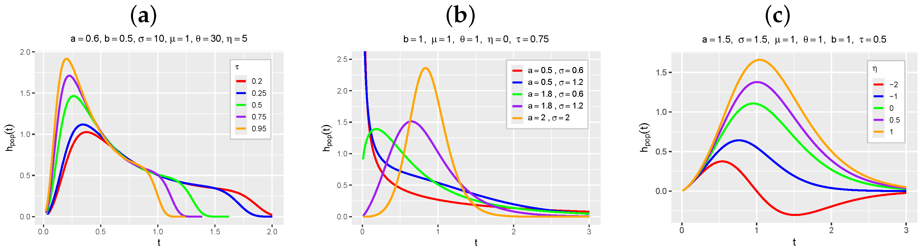
Figure 1 displays the hazard rate function (hrf) plots of the NBGOLLWQ model for selected parameter settings. In Figure 1a, the curves correspond to distinct quantile-parameterized GOLLWQ models indexed by different fixed values of $\tau$, where $\mu$ represents the corresponding $\tau$th quantile in each model. Figure 1b,c illustrate the effects of varying the remaining model parameters while keeping $\tau$ fixed. These plots demonstrate the high flexibility of the proposed model and show that its parameters can substantially influence the hrf shape, allowing for monotonically decreasing and unimodal hazard functions.

Figure 1. Hazard rate function of the new distribution under different parameter settings.In panel (a), each curve corresponds to a distinct GOLLWQ model indexed by a fixed quantile level $\tau$, with $\mu =1$ representing the corresponding $\tau$th quantile in each model. Panels (b,c) illustrate the effects of varying the shape parameters $(a,\sigma )$ and the dispersion parameter $\eta$, respectively, for fixed values of $\tau$.

3. Regression Model

The unobserved time to the event of interest is right-censored, and let $C_i$ be a censoring time. We observe $Y_i=\min \{T_i,C_i\}$ and let ${\delta }_i=\mathrm{I}(T_i\le C_i)$ be such that ${\delta }_i=1$ if $T_i$ is the recurrence time and ${\delta }_i=0$ if right-censored.

We define a parametric model from (12) through the cure fraction $p_{0i}$ for each individual given by the systematic component

$$\log \left({\displaystyle \frac{p_{0i}}{1-p_{0i}}}\right)={\mathit{x}}_i^{\top }\mathit{\beta }\left(\tau \right)\mathrm{or}{p}_{0i}={\displaystyle \frac{exp\left[{\mathit{x}}_i^{\top }\mathit{\beta }\left(\tau \right)\right]}{1+exp\left[{\mathit{x}}_i^{\top }\mathit{\beta }\left(\tau \right)\right]}},$$

(14)

where $\mathit{\beta }\left(\tau \right)={({\beta }_1\left(\tau \right),\cdots ,{\beta }_p\left(\tau \right))}^{\top }$ is the vector of unknown coefficients (for known quantile $\tau$) and ${\mathbf{x}}_i={(x_{i1},\cdots ,x_{ip})}^{\top }$ represents the covariates. The NBGOLLWQ regression model with cure fraction allows modeling for any known quantile $\tau \in [0,1]$.

Following the line of research of Castro et al. (2009) [10] and Cordeiro et al. (2016) [11], we also consider the re-parameterized NB distribution for $\eta \ge -1$, where ${\theta }_i=(p_{0i}^{-\eta }-1)/\eta$ if $\eta \ne 0$, and ${\theta }_i=-\log \left(p_{0i}\right)$ if $\eta =0$.

Under this approach, the improper functions in (12) and (13) reduce to

$$S_{\mathrm{pop}}\left(y_i\right)=\left\{\begin{array}{cc}{\left\{1+{\displaystyle \frac{(p_{0i}^{-\eta }-1){\kappa }^{ab}\left(y_i\right)}{{\kappa }^{ab}\left(y_i\right)+{\left[1-{\kappa }^b\left(y_i\right)\right]}^a}}\right\}}^{-1/\eta },\mathrm{if}\eta \ne 0\hfill & \\ p_{0i}^{\left\{{\displaystyle \frac{{\kappa }^{ab}\left(y_i\right)}{{\kappa }^{ab}\left(y_i\right)+{\left[1-{\kappa }^b\left(y_i\right)\right]}^a}}\right\}},\mathrm{if}\eta =0\hfill & \end{array}\right.$$

(15)

and

$$f_{\mathrm{pop}}\left(y_i\right)=\left\{\begin{array}{cc}{\left\{1+{\displaystyle \frac{(p_{0i}^{-\eta }-1){\kappa }^{ab}\left(y_i\right)}{{\kappa }^{ab}\left(y_i\right)+{\left[1-{\kappa }^b\left(y_i\right)\right]}^a}}\right\}}^{-1/\eta -1}\left({\displaystyle \frac{p_{0i}^{-\eta }-1}{\eta }}\right)\times \hfill & \\ {\displaystyle \frac{ab\sigma w(a,b,\tau ){y_i}^{\sigma -1}[1-\kappa \left(y_i\right)]{\kappa }^{ab-1}\left(y_i\right){\left[1-{\kappa }^b\left(y_i\right)\right]}^{a-1}}{{\mu }^{\sigma }{\left\{{\kappa }^{ab}\left(y_i\right)+{\left[1-{\kappa }^b\left(y_i\right)\right]}^a\right\}}^2}},\mathrm{if}\eta \ne 0\hfill & \\ p_{0i}^{\left\{{\displaystyle \frac{{\kappa }^{ab}\left(y_i\right)}{{\kappa }^{ab}\left(y_i\right)+{\left[1-{\kappa }^b\left(y_i\right)\right]}^a}}\right\}}\times \hfill & \\ {\displaystyle \frac{[-\log \left(p_{0i}\right)]ab\sigma w(a,b,\tau ){y_i}^{\sigma -1}[1-\kappa \left(y_i\right)]{\kappa }^{ab-1}\left(y_i\right){\left[1-{\kappa }^b\left(y_i\right)\right]}^{a-1}}{{\mu }^{\sigma }{\left\{{\kappa }^{ab}\left(y_i\right)+{\left[1-{\kappa }^b\left(y_i\right)\right]}^a\right\}}^2}},\mathrm{if}\eta =0\hfill & \end{array}\right.$$

(16)

where

$$\begin{array}{c}\hfill \kappa \left(y_i\right)=1-exp\left[-w(a,b,\tau ){\left({\displaystyle \frac{y_i}{\mu }}\right)}^{\sigma }\right]\mathrm{and}\end{array}$$

$$\begin{array}{c}\hfill w(a,b,\tau )=-\log \left\{1-{\left[{\displaystyle \frac{{\tau }^{1/a}}{{(1-\tau )}^{1/a}+{\tau }^{1/a}}}\right]}^{1/b}\right\}.\end{array}$$

Equation (16) is called the NBGOLLWQ regression model with cure fraction.

Given $(y_1,{\delta }_1,{\mathbf{x}}_1),\cdots ,(y_n,{\delta }_n,{\mathbf{x}}_n)$, the likelihood function for $\mathit{\psi }={(\eta ,a,b,\mu ,\sigma ,{\mathit{\beta }}^{\top })}^{\top }$ and $\eta \ge -1$ follows from Equations (14)–(16) as

$$L\left(\mathit{\psi }\right)\propto \left\{\begin{array}{cc}{\displaystyle {\prod }_{i=1}^n}{\left\{\left({\displaystyle \frac{p_{0i}^{-\eta }-1}{\eta }}\right){\displaystyle \frac{ab\sigma w(a,b,\tau )y_i^{\sigma -1}[1-\kappa \left(y_i\right)]{\kappa }^{ab-1}\left(y_i\right){\left[1-{\kappa }^b\left(y_i\right)\right]}^{a-1}}{{\mu }^{\sigma }{\left\{{\kappa }^{ab}\left(y_i\right)+{\left[1-{\kappa }^b\left(y_i\right)\right]}^a\right\}}^2}}\right\}}^{{\delta }_i}\hfill & \\ {\left\{1+{\displaystyle \frac{(p_{0i}^{-\eta }-1){\kappa }^{ab}\left(y_i\right)}{{\kappa }^{ab}\left(y_i\right)+{\left[1-{\kappa }^b\left(y_i\right)\right]}^a}}\right\}}^{-{\delta }_i(1/\eta +1)},\mathrm{if}\eta \ne 0\hfill & \\ {\displaystyle {\prod }_{i=1}^n}{\left\{{\displaystyle \frac{-\left[\log \left(p_{0i}\right)\right]ab\sigma w(a,b,\tau )y_i^{\sigma -1}[1-\kappa \left(y_i\right)]{\kappa }^{ab-1}\left(y_i\right){\left[1-{\kappa }^b\left(y_i\right)\right]}^{a-1}}{{\mu }^{\sigma }{\left\{{\kappa }^{ab}\left(y_i\right)+{\left[1-{\kappa }^b\left(y_i\right)\right]}^a\right\}}^2}}\right\}}^{{\delta }_i}\hfill & \\ p_{0i}^{\left\{{\displaystyle \frac{{\kappa }^{ab}\left(y_i\right)}{{\kappa }^{ab}\left(y_i\right)+{\left[1-{\kappa }^b\left(y_i\right)\right]}^a}}\right\}},\mathrm{if}\eta =0\hfill & \end{array}\right.$$

(17)

The MLE of $\mathit{\psi }$ is found by maximizing the log-likelihood (17) using SAS’s 9.4 NLMIXED procedure [12] or R’s version 4.5.1, Optim function [13]. Starting values for the optimization process are determined by setting $a=b=1$ and fitting the reduced model. We conduct statistical inference for the parameters using the classical asymptotic properties of MLEs.

4. Machine Learning Methods

The primary goal of machine learning is to predict future outcomes. To ensure accuracy, data is partitioned into training and testing sets, allowing algorithms to identify patterns and facilitate automated decision-making.

There are two primary types of machine learning: supervised learning, which uses predictor variables to forecast a response (via classification or regression), and unsupervised learning, which identifies patterns in unlabeled data. Survival analysis specifically employs supervised learning through regression modeling.

4.1. Random Survival Forests

Random survival forest (RSF) (Ishwaran et al., 2008 [14]) is a non-parametric tree-ensemble algorithm designed for right-censored survival analysis. The method constructs an ensemble of survival trees utilizing bootstrap sampling of the data. To minimize tree correlation and maximize diversity, node splitting relies on random feature subsets and splitting rules tailored for censored data.

Each tree is generated as follows:

1.

Generate a bootstrap sample (with replacement).

2.

Randomly choose a subset of variables for each split.

3.

Use a division criterion that maximizes the difference in survival between nodes. The log-rank test is used for this purpose:

$$L(x,s)={\displaystyle \frac{{\displaystyle {\displaystyle \sum _{k=1}^D}\left(d_{k,l}-Y_{k,l}\frac{d_k}{Y_k}\right)}}{\sqrt{{\displaystyle {\displaystyle \sum _{k=1}^D}{Y}_{k,l}\frac{Y_k-Y_{k,l}}{Y_k-1}\left(1-\frac{d_k}{Y_k}\right)d_k}}}},$$

(18)

where $d_{k,l}$ and $Y_{k,l}$ are the number of events and the number at risk in the left child node at time $t_k$, respectively.

4.

Continue the recursive splitting of the nodes until a minimum number of samples in a terminal node or a maximum tree depth is satisfied.

5.

Estimate the cumulative hazard function at each terminal node using the Nelson–Aalen estimator:

$${\widehat{H}}_h\left(t\right)=\sum _{t_{l,h}\le t}{\displaystyle \frac{d_{l,h}}{Y_{l,h}}},$$

(19)

where $d_{l,h}$ and $Y_{l,h}$ are, respectively, the number of events and the number at risk at time $t_{l,h}$ in node h.

6.

Combine the B trees to obtain the final ensemble prediction:

$${\widehat{H}}_{\mathrm{rsf}}(t\mid x_i)={\displaystyle \frac{1}{B}}{\displaystyle \sum _{b=1}^B}{\widehat{H}}_b(t\mid x_i),{\widehat{S}}_{\mathrm{rsf}}(t\mid x_i)=exp\left(-{\displaystyle \frac{1}{B}}{\displaystyle \sum _{b=1}^B}{\widehat{H}}_b(t\mid x_i)\right).$$

(20)

RSF does not rely on the proportional hazards assumption, offering greater flexibility across diverse datasets. When nodes are split, the algorithm evaluates possible thresholds and selects the split point that maximizes survival differences using the log-rank test.

Variable importance can be quantified using Permutation Importance (VIMP). This method measures the marginal contribution of a predictor by estimating the increase in prediction error when its values are randomly permuted. Higher VIMP values denote a stronger reliance by the model and, consequently, greater predictive relevance.

4.2. Validation of the Model: Cross-Validation

The k-fold cross-validation divides data into k subsets. The model trains on all but one subset, tests on the held-out subset, and rotates until all subsets are used. This prevents overfitting and accurately evaluates performance. Common values are $k=5$ and $k=10$.

4.3. Concordance Index (C-Index)

The concordance index evaluates survival models considering censoring. Measures the proportion of valid pairs with correct predictions (longer predicted survival times for those who survived longer). Values above 0.5 indicate acceptable performance.

5. Simulation Study

We utilize simulations in R to examine the MLE properties of the NBGOLLWQ regression framework. The event of interest, T, was modeled using a GOLLWQ distribution with s parameters: $a=2$, $b=0.5$, $\mu =4$ and $\sigma =0.05$.

The simulation study was conducted separately for the fixed quantile levels $\tau =0.25$, $\tau =0.50$, and $\tau =0.75$. Each value of $\tau$ defines a distinct quantile-parameterized GOLLWQ model. In all scenarios, $\mu =4$ denotes the corresponding $\tau$th quantile of the respective model. Therefore, the simulations do not represent different quantiles of the same distribution, but rather three distinct GOLLWQ models indexed by fixed values of $\tau$.

The values of the random variable T are generated from Equation (9), and the number of causes $M_i$ of the event is generated from the NB distribution with $\eta =12$ and ${\theta }_i$, that is,

$${\theta }_i=(p_{0i}^{-\eta }-1)/\eta \mathrm{and}{p}_{0i}={\displaystyle \frac{exp({\beta }_0\left(\eta \right)+{\beta }_1\left(\eta \right)x_i)}{1+exp({\beta }_0\left(\eta \right)+{\beta }_1\left(\eta \right)x_i)}}.$$

The values of the covariate $x_i$ are generated from a Bernoulli distribution with parameter 0.5 and ${\beta }_0=-1.0$ and ${\beta }_1=2.0$.

We generate censoring times C from a uniform $(0,k)$, with k tuned to produce a 53% censoring rate. Observed survival times are calculated as $y_i=\min (t_i,c_i)$ following the steps below:

1.

Generate $M_i\sim$NB($\eta ,{\theta }_i$).

2.

If $M_i=0$, then $t_i=\infty$; otherwise, generate $z_i\sim \mathrm{GOLLWQ}(a,b,\mu ,\sigma \mid \tau )$ to find $t_i=\min (Z_1,\cdots ,Z_{D_i})$ for every i.

3.

The censoring variable $c_i$ is generated from $C\sim$U$(0,k)$, where k is the cure fraction in the sample.

4.

Obtain $y_i=\min (t_i,c_i)$. If $y_i<c_i$, ${\delta }_i=1$; otherwise, ${\delta }_i=0$.

Table 1 presents the average estimates (AE), biases, root mean square errors (RMSE), and coverage probabilities (CP) based on $B=1000$ simulations. These were calculated for $n=150$, 300, 450 and 600 under three distinct quantile-parameterized models corresponding to the fixed quantile levels $\tau =0.25$, $\tau =0.50$, and $\tau =0.75$, using R’s Optim routine.

Table 1. Outcomes from the fitted NBGOLLWQ regression model.

		$\mathit{\tau }$ = 0.25				$\mathit{\tau }$ = 0.50				$\mathit{\tau }$ = 0.75
$\mathit{n}$	${\mathit{\psi }}_{\mathit{n}}$	AE	Bias	RMSE	CP	AE	Bias	RMSE	CP	AE	Bias	RMSE	CP
	${\beta }_0$	−0.9828	0.0171	0.2544	0.9580	−1.0090	−0.0090	0.2489	0.9450	−1.0147	−0.0147	0.2544	0.9500
	${\beta }_1$	2.0535	0.0535	0.2541	0.9400	2.0664	0.0664	0.2757	0.9390	2.0647	0.0647	0.2932	0.9490
	a	2.8567	0.8567	2.0417	0.9120	2.7903	0.7903	1.9618	0.9230	2.6633	0.6633	1.7951	0.9320
150	b	0.8436	0.3436	0.9856	0.9070	0.7490	0.2490	0.7095	0.9240	0.6953	0.1953	0.5402	0.9150
	$\sigma$	0.0462	−0.0037	0.0226	0.9550	0.0490	−0.0009	0.0279	0.9720	0.0522	0.0022	0.0313	0.9740
	$\mu$	3.8734	−0.1265	0.6734	0.9440	3.7497	−0.2502	1.3752	0.9290	3.6810	−0.3189	1.7342	0.8890
	$\eta$	15.6711	3.6711	8.0077	0.9080	15.1285	3.1285	7.9712	0.9210	15.2567	3.2567	7.8214	0.9120
	${\beta }_0$	−0.9942	0.0057	0.1933	0.9470	−1.0036	−0.0036	0.1792	0.9530	−1.0036	−0.0036	0.1697	0.9440
	${\beta }_1$	2.0374	0.0374	0.1845	0.9410	2.0401	0.0401	0.1930	0.9400	2.0448	0.0448	0.2132	0.9440
	a	2.4893	0.4893	1.4292	0.9240	2.5218	0.5218	1.3960	0.9510	2.4461	0.4461	1.3279	0.9280
300	b	0.6824	0.1824	0.5295	0.9320	0.6522	0.1522	0.4314	0.9180	0.6017	0.1017	0.3510	0.9290
	$\sigma$	0.0473	−0.0026	0.0190	0.9540	0.0484	−0.0015	0.0250	0.9690	0.0518	0.0018	0.0263	0.9730
	$\mu$	3.9240	−0.0759	0.6717	0.9410	3.7138	−0.2861	1.5085	0.9080	3.7769	−0.2230	1.9642	0.8860
	$\eta$	13.8062	1.8062	5.0446	0.9340	13.8211	1.8211	5.3445	0.9300	13.4550	1.4553	4.9476	0.9320
	${\beta }_0$	−0.9951	0.0048	0.1564	0.9470	−1.0034	−0.0034	0.1397	0.9520	−1.0035	−0.0035	0.1433	0.9500
	${\beta }_1$	2.0232	0.0232	0.1480	0.9480	2.0313	0.0313	0.1596	0.9480	2.0319	0.0319	0.1681	0.9440
	a	2.3982	0.3982	1.2136	0.9170	2.3813	0.3813	1.0925	0.9250	2.4131	0.4131	1.0921	0.9170
450	b	0.6151	0.1151	0.3617	0.9380	0.5959	0.0959	0.3019	0.9260	0.5564	0.0564	0.2629	0.9320
	$\sigma$	0.0458	−0.0041	0.0210	0.9760	0.0466	−0.0033	0.0239	0.9680	0.0500	0.0000	0.0239	0.9680
	$\mu$	3.9237	−0.0762	0.7443	0.9440	3.8154	−0.1845	1.5629	0.9060	3.8689	−0.1310	2.1585	0.9610
	$\eta$	13.0395	1.0395	3.3545	0.9330	12.8732	0.8732	3.2888	0.9430	12.9941	0.9941	3.6341	0.9410
	${\beta }_0$	−0.9965	0.0034	0.1356	0.9410	−0.9999	0.0001	0.1284	0.9450	−1.0010	−0.0019	0.1250	0.9410
	${\beta }_1$	2.0183	0.0183	0.1237	0.9460	2.0234	0.02348	0.1344	0.9470	2.0199	0.0199	0.1412	0.9440
	a	2.3556	0.3556	1.0069	0.9210	2.3367	0.3367	0.9350	0.9210	2.2890	0.2890	0.8570	0.9230
600	b	0.6120	0.1120	0.3171	0.9370	0.5761	0.0761	0.2524	0.9250	0.5453	0.0453	0.2147	0.9360
	$\sigma$	0.0436	−0.0063	0.0185	0.9580	0.0465	−0.0034	0.0212	0.9640	0.0498	−0.0001	0.0221	0.9630
	$\mu$	3.9250	−0.0749	0.7241	0.9310	3.8919	−0.1080	1.6392	0.9020	4.0977	0.0977	2.2440	0.9550
	$\eta$	12.8021	0.8021	2.7374	0.9300	12.7299	0.7299	2.6829	0.9340	12.7589	0.7589	2.7056	0.9300

Coverage probability is the chance that your confidence interval actually captures the true parameter you are trying to measure. Practically, if we ran our experiment hundreds of times, our intervals would contain the correct value a certain percentage of the time (e.g., $95\%$ for a $95\%$ confidence interval).

The results demonstrate that the AEs approach the true parameters, while biases and RMSEs decrease as n grows. Moreover, because the CP values consistently approximate 95%, it is clear that the asymptotic normal distribution effectively models the distribution of the MLEs.

6. Application: Prostate Cancer Recurrence Data

Prostate cancer typically develops slowly and presents no symptoms in its early stages. According to the American Cancer Society, about 1 in 8 men will be diagnosed in their lifetime. The risk increases rapidly after age 50 and is heavily influenced by family history and race/ethnicity.

There has been a worrying increase in the number of metastatic (advanced-stage) prostate cancer cases, although there has been a decrease in the incidence of its localized type. Despite advances in treatment, prostate cancer still causes a significant number of deaths. In 2024, more than 35,000 men died from the disease in the US. This number represents approximately 5.8% of all cancer deaths in the country.

We applied the NBGOLLWQ regression model to data from 1324 localized prostate cancer patients who underwent open radical prostatectomy performed by a single surgeon at the Cleveland Clinic between 1987 and 2003. This dataset included 1096 censored and 228 uncensored observations.

The explanatory variables below are determined for each patient (for $i=1,\dots ,1324$):

• $t_i$: number of months the patient has remained cancer-free following prostatectomy;
• ${\delta }_i:$ equals 1 if the event occurs and 0 refers to censored;
• $x_{i1}:$ patient receives hormone therapy prior prostatectomy (yes = 1 and no = 0);
• $x_{i2}:$ PSA value (in ng/mL) before prostatectomy;
• $x_{i3}:$ extracapsular extension (yes = 1, no = 0);
• $x_{i4}:$ seminal vesicle invasion (yes = 1, no = 0);
• $x_{i5}:$ Gleason sum ([4,7) = 0, versus 7 = 1);
• $x_{i6}:$ Gleason sum ([4,7) = 0, versus [8,10] = 1);
• $x_{i7}:$ lymph node involvement (neg = 1, pos = 0);
• $x_{i8}:$ surgical margin status (yes = 1, no = 0).

Some considerations regarding these covariates:

• Neoadjuvant hormonal therapy ($x_{i1}$) in prostate cancer treatment involves the use of medications to block or reduce the production of androgens like testosterone prior to primary treatments such as surgery or radiation. Also known as androgen deprivation therapy, this approach is designed to shrink tumor volume and downstage the disease, thereby facilitating surgical removal or sensitizing the tumor to radiation therapy.
• Prostate-specific antigen (PSA) ($x_{i2}$) quantifies a protein synthesized by the prostate. Elevated levels can signal cancer but are not definitive. Because noncancerous conditions also elevate this marker, additional diagnostic tools are required to confirm the disease.
• Extracapsular extension $\left(x_{i3}\right)$ occurs when a tumor breaks through the outer boundary or capsule of an organ or lymph node, invading surrounding tissues. In oncology, this indicates a more aggressive cancer and is a critical factor for determining disease stage, planning treatments, and assessing patient prognosis.
• Invasion of the seminal vesicle $\left(x_{i4}\right)$, in the context of diseases like prostate cancer, means that the tumor has spread beyond the prostate gland and into the seminal vesicles. This marks a more advanced stage of the disease, indicating that the cancer is locally aggressive.
• The Gleason sum $(x_{i5},x_{i6})$ refers to the aggressiveness of prostate cancer based on the appearance of cancer cells in biopsies. The Gleason score (2–10) is the sum of the two most dominant malignancy grades observed in a biopsy. Elevated scores correlate with increased tumor aggressiveness and a poorer prognosis.
• Lymph node involvement ($x_{i7}$) means prostate cancer cells have traveled beyond the primary tumor into the lymphatic system. This indicates regional spread, suggesting the cancer may advance or has already metastasized to other areas of the body
• Surgical margin status $\left(x_{i8}\right)$ indicates the presence or absence of malignant cells at the borders of excised tissue. Confirming whether margins are “clear” or “positive” is critical for evaluating complete tumor removal, determining prognosis, and guiding subsequent treatment plans.

The analysis starts by conditioning exclusively on the response variable and censoring. As detailed in Table 2, we evaluate models based on Global Deviance (GD), Akaike Information Criterion (AIC), and cure rate estimates. The NBGOLLWQ model, with $\tau =0.75$, registers the lowest GD and AIC values and is thus selected as the best-fitting model.

Table 2. Selection criteria and cure rate of the NBGOLLWQ model for three values of $\tau$.

Models	GD	AIC	${\widehat{\mathit{p}}}_0$
NBGOLLWQ ($\tau =0.25$)	3015.708	3027.708	0.3973
NBGOLLWQ ($\tau =0.50$)	3015.030	3027.030	0.5912
NBGOLLWQ ($\tau =0.75$)	3013.800	3025.800	0.6160

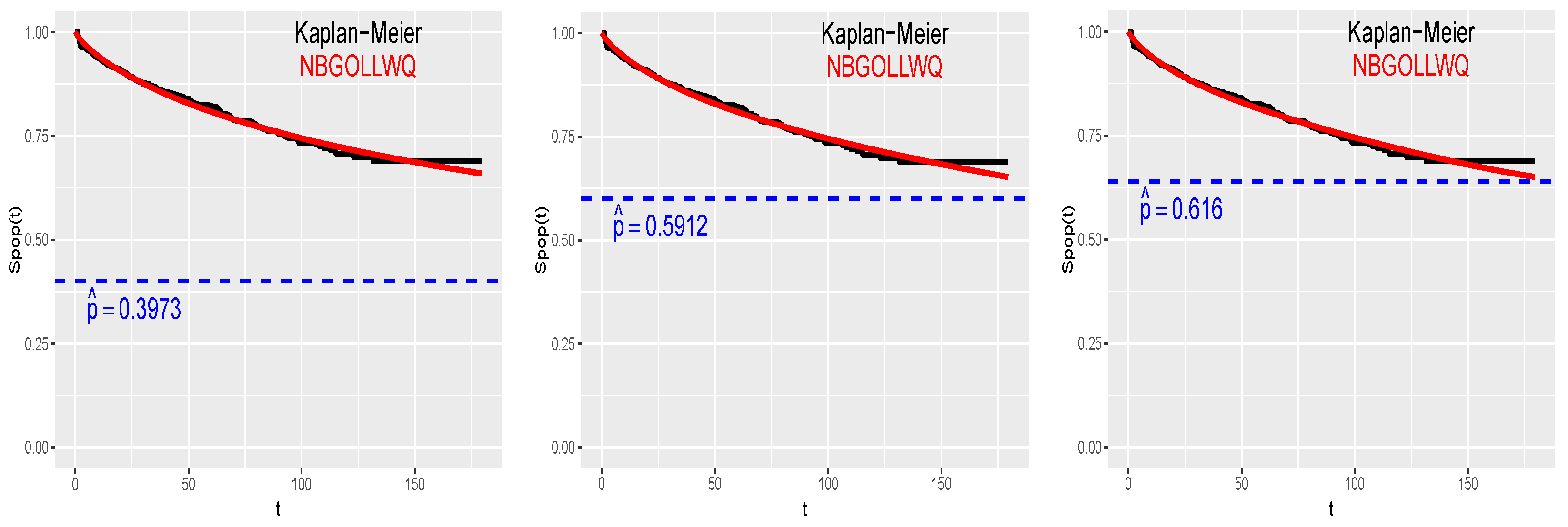
Figure 2 displays the empirical and estimated survival functions, along with the estimated cure rates for the NBGOLLWQ models. Among these, this model with $\tau =0.75$ provides the optimal fit for the data, indicating that approximately 62% of patients are cured.

Figure 2. Empirical and estimated survival functions for the NBGOLLWQ model.

Next, we fit the regression model

$$\begin{array}{c}\hfill p_{0i}={\displaystyle \frac{exp\left({\beta }_0\left(\tau \right)+{\sum }_{j=1}^8{\beta }_j\left(\tau \right)x_{ij}\right)}{1+exp\left({\beta }_0\left(\tau \right)+{\sum }_{j=1}^8{\beta }_j\left(\tau \right)x_{ij}\right)}},\end{array}$$

to the current data. The MLEs of the parameters are calculated through the NLMixed procedure in SAS 9.4 and Optim routine of the R software version 4.5.1. Iterative maximization of the logarithm of (17) starts with the estimates from the Weibull quantile regression model.

We evaluated the NBGOLLWQ regression model against the nested NBOLLWQ, NBGExpWQ, and NBWQ models across quantiles $\tau =0.25$, $0.50$, and $0.75$. As shown in Table 3, the NBGOLLWQ model achieved the lowest GD and AIC values. Therefore, we selected this model at $\tau =0.75$ for our subsequent data analysis.

Table 3. GD and AIC values for four fitted quantile regression models to prostate cancer data.

		Quantile Regression Models
$\mathit{\tau }$	Values	NBGOLLWQ	NBOLLWQ	NBGExpWQ	NBWQ
0.25	GD	2688.2	2692.1	2689.9	2692.3
	AIC	2716.2	2718.1	2715.9	2716.3
0.50	GD	2691.7	2692.8	2693.0	2694.6
	AIC	2719.7	2718.8	2719.0	2718.6
0.75	GD	2687.5	2694.0	2693.4	2704.2
	AIC	2715.5	2720.0	2719.4	2728.2

Note: Values in bold indicate the smallest value.

Table 4 reports the MLEs, their standard errors (SEs), and the significance levels for the optimal model. While most covariates are statistically significant at the 5% level, covariate x₅ shows marginal significance with a p-value of 0.0552.

Table 4. Findings from the NBGOLLWQ regression model for $\tau =0.75$.

Parameter	Estimate	SE	p-Value	95% Confidence Interval
${\beta }_0$	1.7813	0.5687	0.0018	(0.6656, 2.8969)
${\beta }_1$	−0.6463	0.2441	0.0082	(−1.1252, −0.1674)
${\beta }_2$	−0.0312	0.0133	0.0188	(−0.0572, −0.0052)
${\beta }_3$	−0.8435	0.2005	<0.0001	(−1.2369, −0.4502)
${\beta }_4$	−1.0953	0.2909	0.0002	(−1.6659, −0.5247)
${\beta }_5$	1.0953	0.5365	0.0552	(−0.0230, 2.0818)
${\beta }_6$	−0.9129	0.2144	<0.0001	(−1.3335, −0.4924)
${\beta }_7$	−2.3374	0.3809	<0.0001	(−3.0846, −1.5902)
${\beta }_8$	−1.0417	0.2008	<0.0001	(−1.4357, −0.6478)
$\eta$	0.4204	0.2762	—	(−0.1214, 0.9623 )
a	0.4450	0.1723	—	(0.1070, 0.7830 )
b	0.4880	0.3290	—	(−0.1573, 1.1334 )
$\mu$	96.6536	7.7611	—	(81.4283, 111.88)
$\sigma$	4.5855	1.6666	—	(1.3161, 7.8549 )

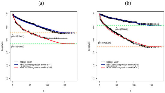
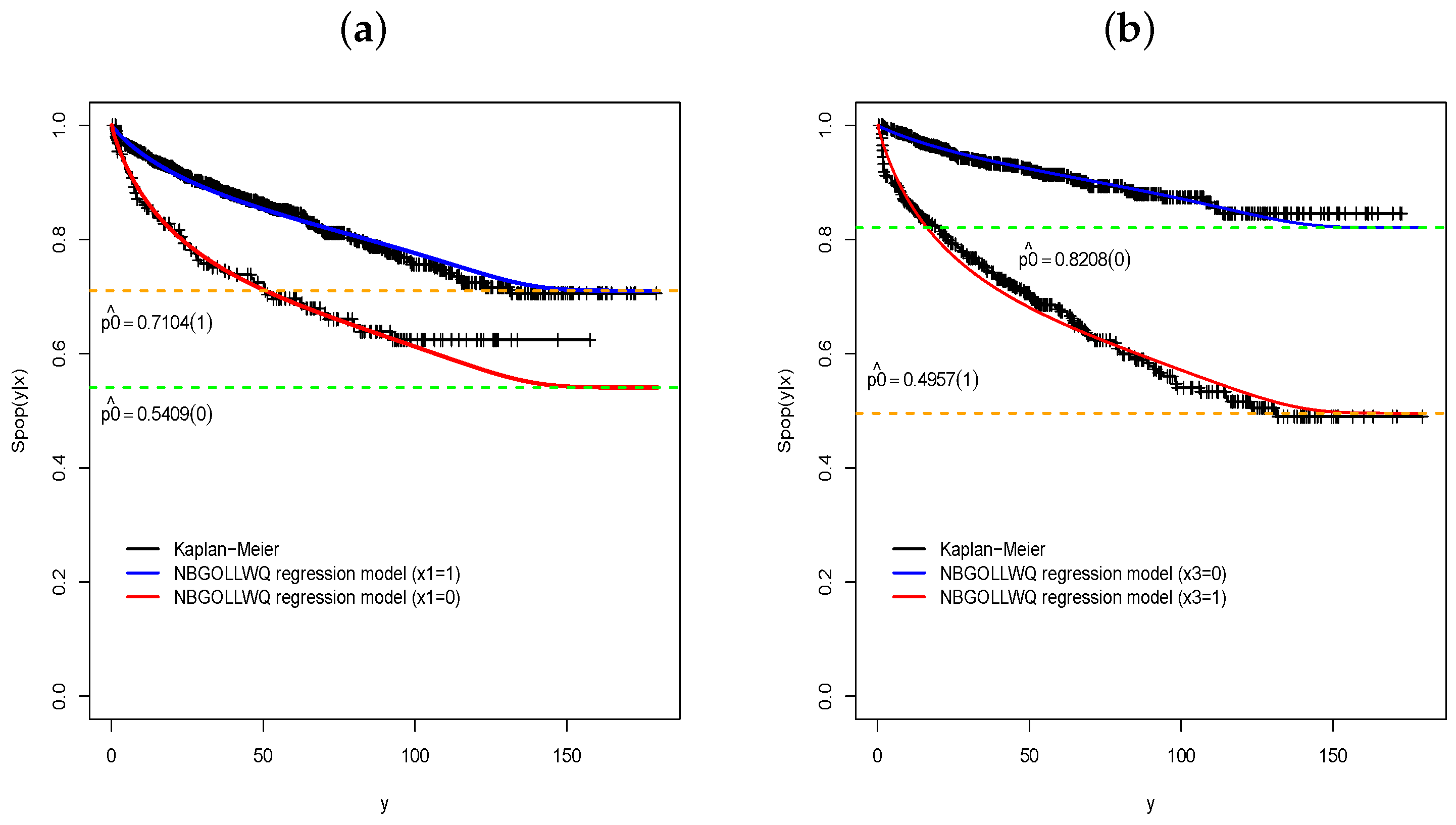
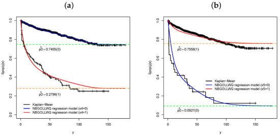
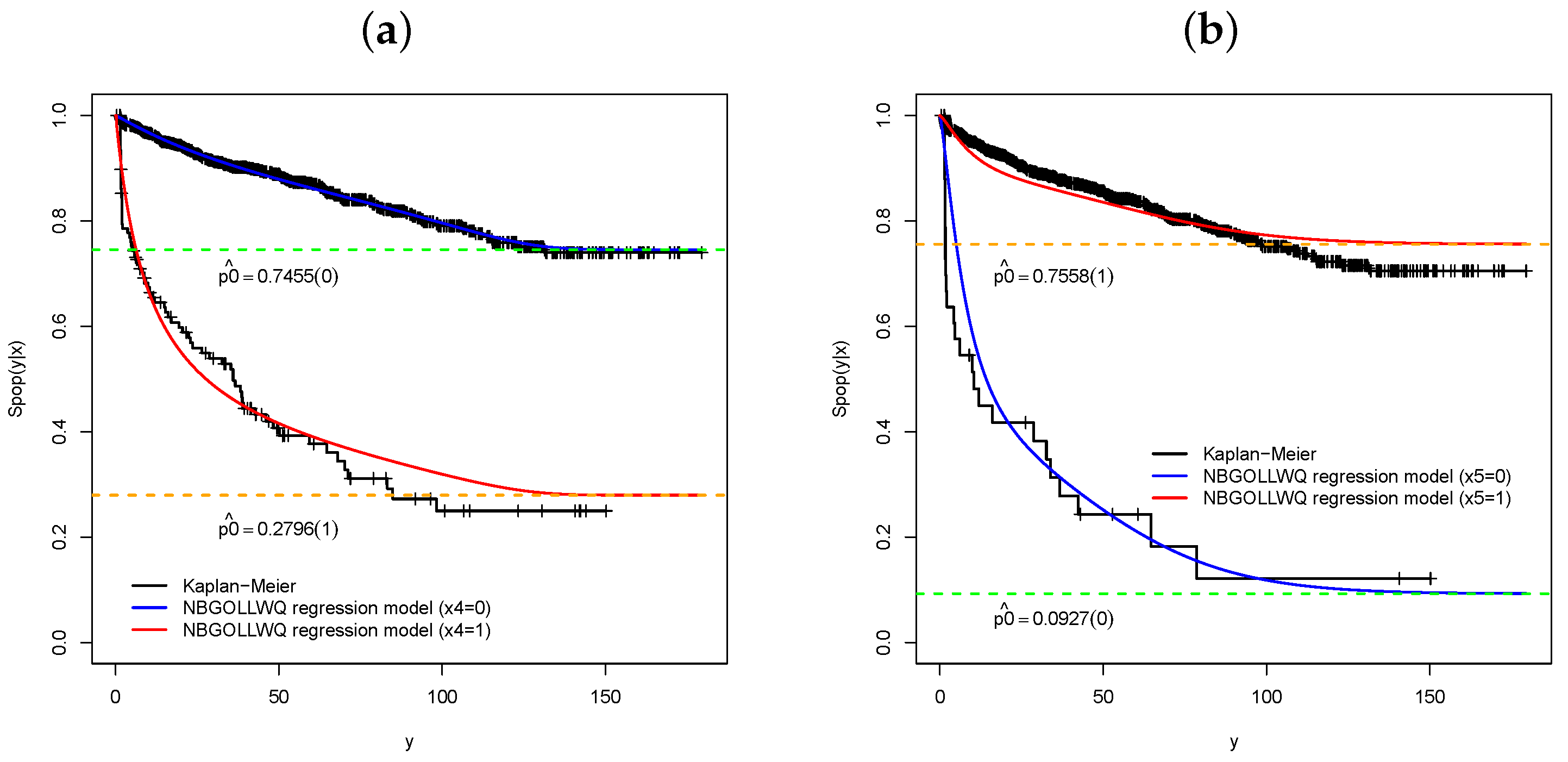
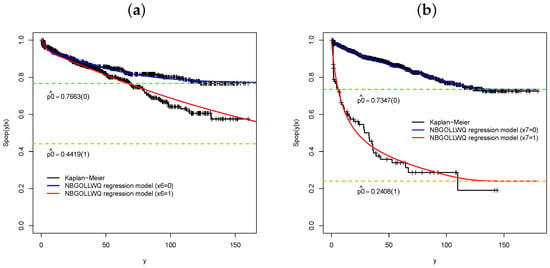
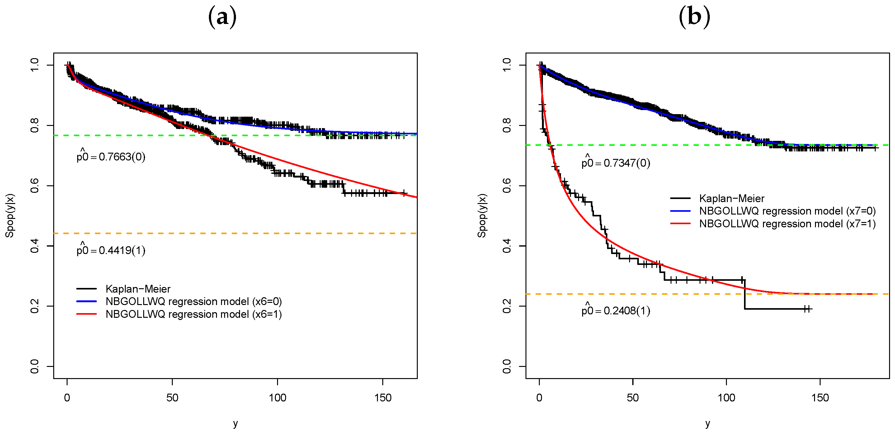
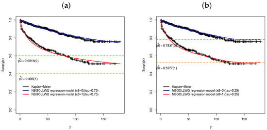
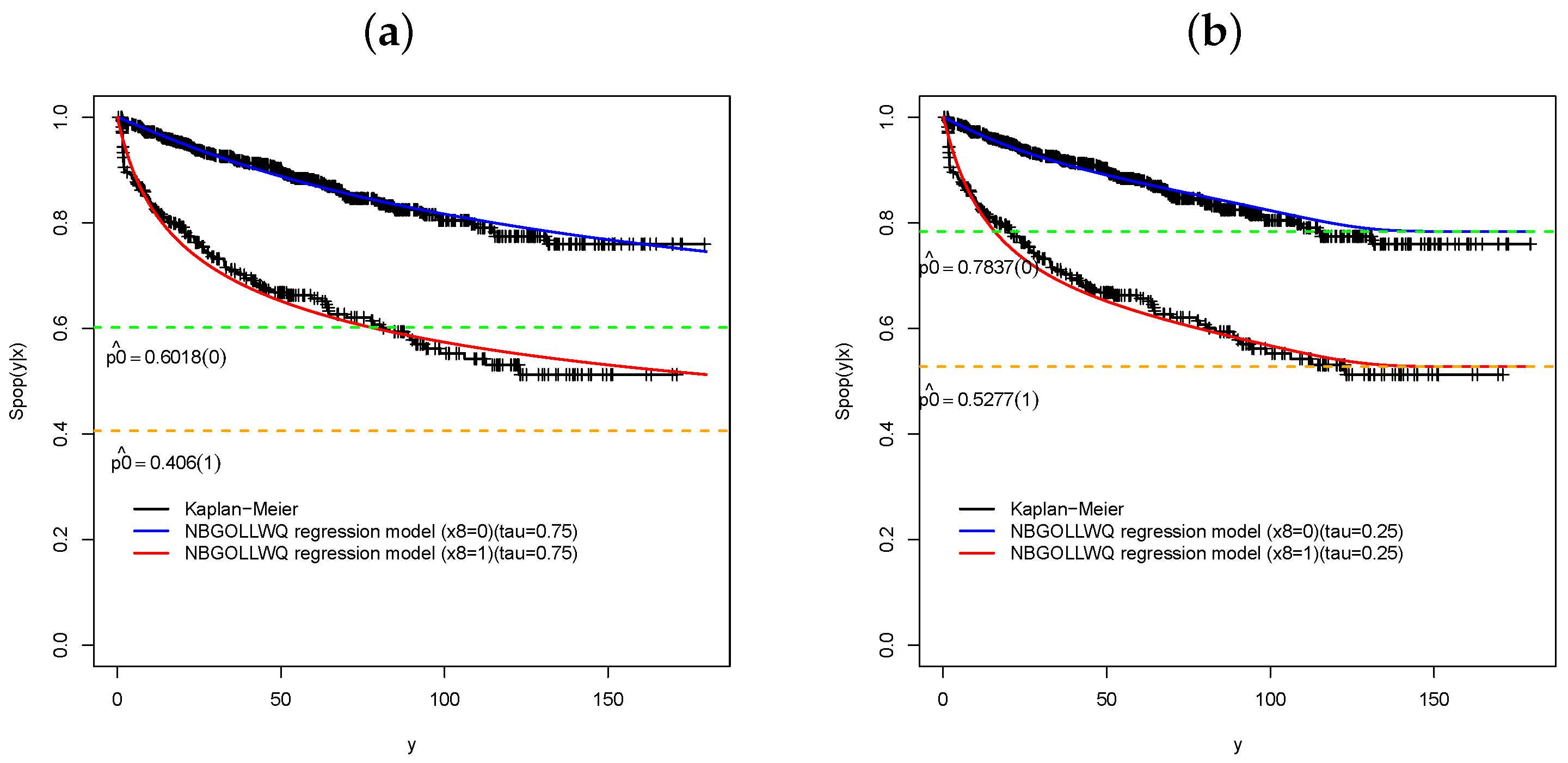
We fitted the NBGOLLWQ regression model for each explanatory variable. Figure 3, Figure 4, Figure 5 and Figure 6 present plots comparing the empirical and estimated survival functions for each predictor.

Figure 3. Plots of the survival functions of the NBGOLLWQ regression model for $\tau =0.75$ and Kaplan–Meier curves: (a) $x_1$; (b) $x_3$.

Figure 4. Plots of the survival functions of the NBGOLLWQ regression model for $\tau =0.75$ and Kaplan–Meier curves: (a) $x_4$; (b) $x_5$.

Figure 5. Plots of the survival functions of the NBGOLLWQ regression model for $\tau =0.75$ and Kaplan–Meier curves: (a) $x_6$; (b) $x_7$.

Figure 6. Plots of the survival functions of the NBGOLLWQ regression for $\tau =0.75$ and Kaplan–Meier curves: (a) $x_6$; (b) $x_8$.

In the following text, some details will be explained.

Interpretations:

• A significant difference in post-prostatectomy disease-free survival is evident between patients who received hormonal therapy and those who did not (Table 4 and Figure 3a). Projections indicate cure rates of approximately $71\%$ for the hormonal therapy cohort and $54\%$ for the untreated cohort.
• The cure rate decreases significantly (5%) when PSA increases.
• Based on Table 4 and Figure 3b, there is a significant difference between the levels of extracapsular extension levels in the lymph nodes to the time without detectable disease after prostatectomy. We also note that for patients who did not have extracapsular extension in the lymph nodes, approximately 82% is expected to be cured, while for patients who had extracapsular extension, 50% is expected to be cured.
• Table 4 and Figure 4a reveal a statistically significant link between gallbladder invasion status and the duration of disease-free survival following a prostatectomy. Specifically, the expected cure rate is $75\%$ for patients without gallbladder invasion, dropping sharply to just $28\%$ for those with reported invasion.
• We classify the covariates $x_5$ and $x_6$ in three levels: [4, 7], 7, and [8, 10]. There is a significant difference between the levels [4, 7) and 7, and [4, 7) and [8, 10]. Figure 4b and Figure 5a reveal that 76% of the patients with Gleason sum in the interval [4, 7] will be cured. For patients with levels of 7 and [8, 10], it is expected that 9% and 34% will be cured, respectively.
• As shown in Table 4 and Figure 5b, lymph node status significantly impacts post-prostatectomy disease-free survival. Patients without lymph node involvement have an expected cure rate of 74%, whereas those with positive nodes face a substantially lower cure rate of 24%.
• Finally, Table 4 highlights a statistically significant difference in cure proportions based on surgical margin status. Figure 6a,b demonstrate that the 0.25 quantile is the most appropriate for modeling covariate $x_8$, as the 0.75 quantile severely underestimates the cure proportion. Consequently, Figure 6b shows that patients who had their tumors completely removed achieved a cure proportion of 78%, whereas those with incomplete tumor removal experienced a drop to approximately 53%.

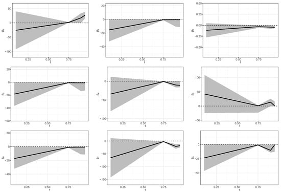
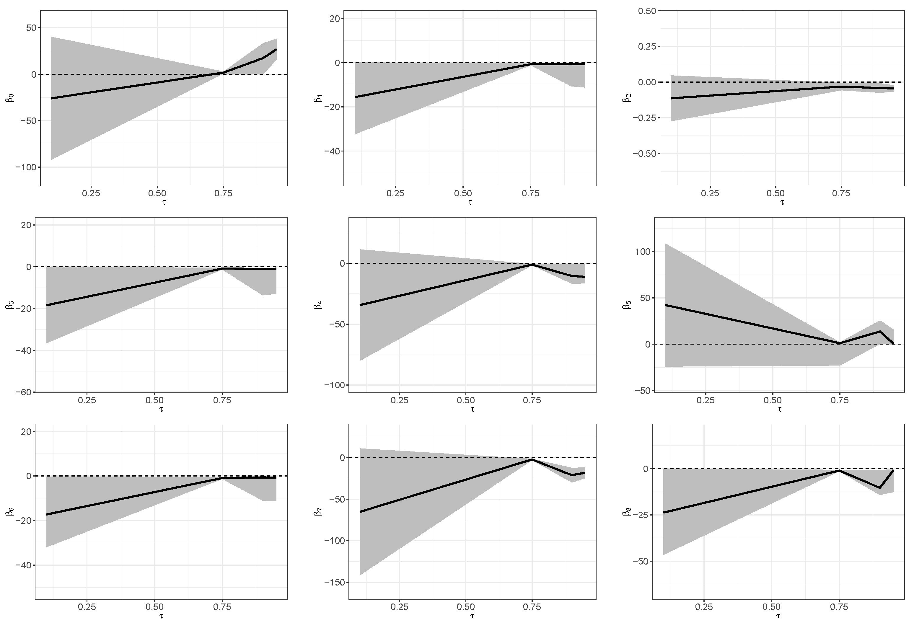
Figure 7 displays the MLEs and corresponding ($95\%$) confidence intervals for the quantile range $[0.01,0.99]$.

Figure 7. Maximum likelihood estimates (MLEs) and 95% CIs for parameters versus $\tau$. The solid black lines represent the parameter estimates, the gray shaded regions correspond to the 95% confidence intervals, and the dashed horizontal lines indicate the reference value zero.

Random Forest

We trained an RF model on survival data to see how well it captures risk over time, tested for the potential presence of a cured subgroup, and compared its predictive accuracy with our proposed parametric model.

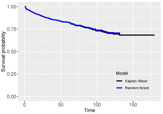
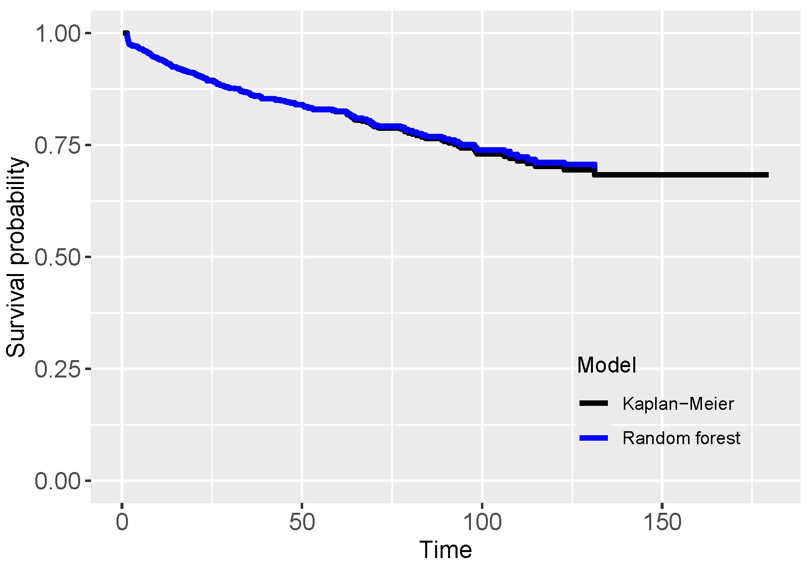
We randomly divided the dataset into an 80% training set and a 20% testing set. Model hyperparameters were optimized using 5-fold cross-validation on the training data. Once the optimal parameters were determined, the estimated survival curve was generated, as displayed in Figure 8. The generated nonparametric survival curve accurately tracks the observed data until the final event, reliably capturing sample behavior. However, unlike parametric alternatives, random forest fails to explicitly estimate the cured fraction. This drawback can limit its application in clinical or scientific settings where quantifying cured patients is essential.

Figure 8. Survival curve estimated by the RF model and Kaplan–Meier curve.

We compared model predictive accuracy using the concordance index (c-index). The RF model achieved a c-index of 0.83, significantly outperforming the NBGOLLWQ model, which scored 0.60. While RF is better at ranking temporal risk, this model offers the distinct interpretive advantage of explicitly estimating the cure fraction.

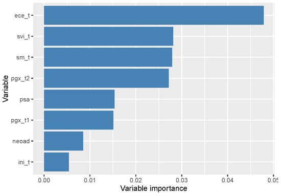
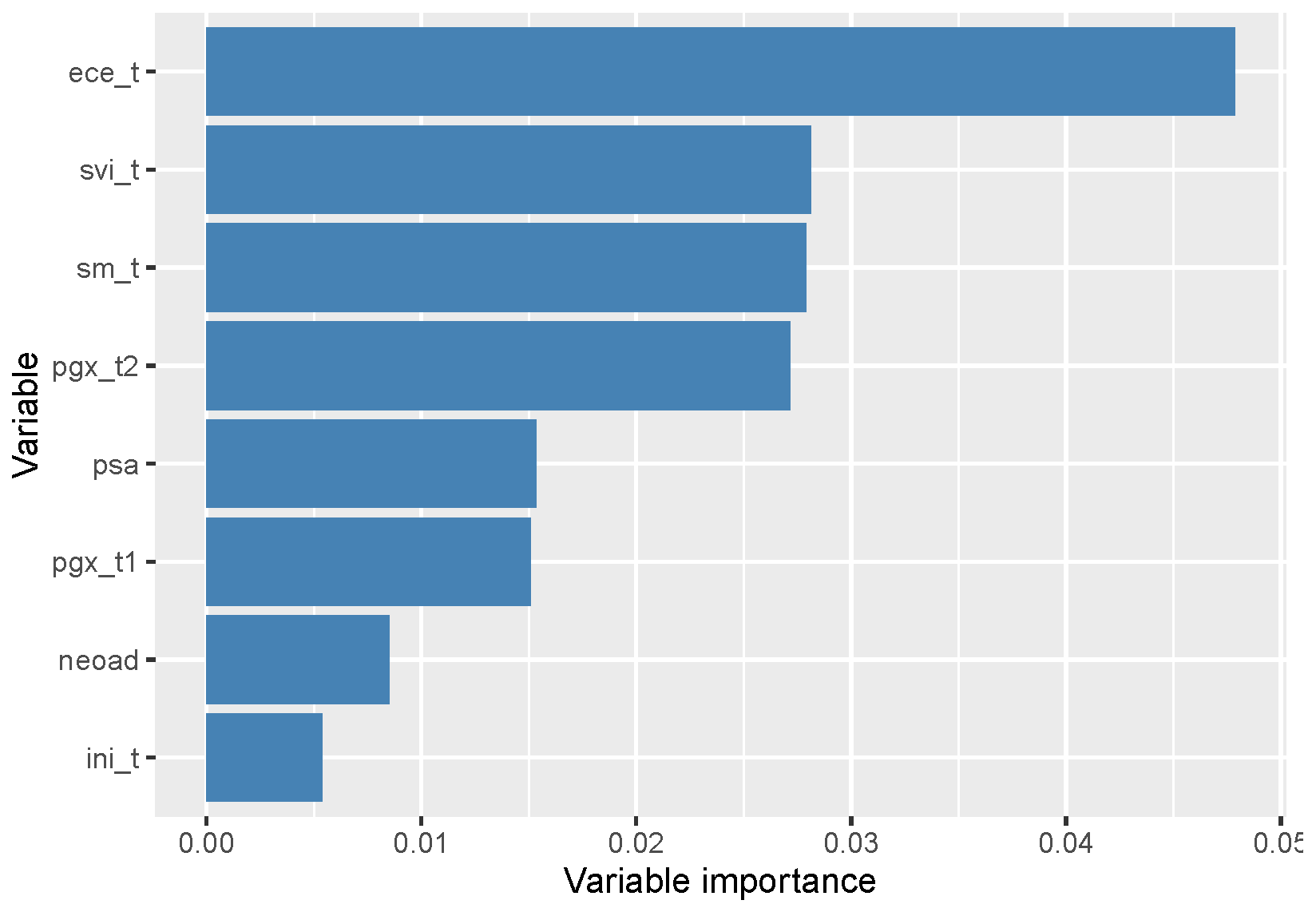
Figure 9 displays variable importance for the random forest model using the permutation method. This approach determines each predictor’s significance by measuring how much the model’s error increases when that specific variable’s data is shuffled.

Figure 9. Importance of variables in predicting survival time, as estimated by the RF model. Higher values indicate greater contribution of the variable to the accuracy of the model.

Extracapsular extension ($x_3$) emerges as the most critical variable. Its substantial impact indicates a strong association with the time to the event, establishing it as a vital prognostic marker. Following this, seminal vesicle invasion ($x_4$) and surgical margin status ($x_8$) also demonstrate a significant influence on the model.

These pathological features indicate localized disease extension and an elevated risk of recurrence. Furthermore, an elevated Gleason sum ($x_7$) of 8–10 emerged as a highly significant variable, showing that more aggressive histological grades strongly correlate with adverse clinical outcomes.

The pre-surgical PSA value ($x_2$) and a Gleason score of 7 ($x_6$) had intermediate importance. The use of neoadjuvant hormone therapy ($x_1$) and negative lymph node invasion ($x_5$) showed less relative importance, although they still contributed some information to the model.

These results highlight key risk factors, providing a foundation for future model refinement and clinical interpretation. Additionally, excluding variables with low importance can help build more streamlined and efficient models.

7. Concluding Remarks

To better capture latent competing risks, we combined the highly flexible generalized odd log-logistic Weibull (GOLLW) distribution with the negative binomial (NB) distribution. This led to the development of the NBGOLLWQ model, an innovative quantile regression framework designed for survival data with a cure fraction.

By explicitly incorporating cured fractions and flexible quantile modeling, this approach broadens standard survival regression, delivering a more detailed analysis of conditional survival distributions. Following a maximum likelihood estimation procedure and Monte Carlo simulations, we applied our proposed methodology to prostate cancer data. The findings confirm that the NBGOLLWQ model successfully explains the cure fraction and measures the influence of clinically relevant covariates on various survival quantiles.

Among the evaluated quantile regression models, the $\tau =0.75$ threshold delivered the most robust fit, identifying a cure fraction of approximately 62%. Additionally, the model provided valuable clinical insights by clearly separating patients into distinct high- and low-risk categories based on their specific covariate patterns.

We compared our proposed model with a random survival forest. Although the random forest showed superior predictive performance (c-index = 0.83 versus 0.60), it lacks the ability to estimate the cure fraction. This limitation makes it less interpretable in medical contexts, where identifying long-term survivors is critical. Conversely, the NBGOLLWQ model delivers a strong balance of parametric flexibility and clear interpretability.

For future research, we plan to develop Bayesian versions of our model, extend it to include covariates across other parameters, and explore quantile-based model selection. Future objectives include establishing local influence diagnostics to assess model robustness and developing residual analysis methods specifically for regression models with a cure fraction. Machine learning frameworks can be broadened to accommodate long-term survivor populations in subsequent analyses.

Furthermore, we propose the development of local influence analysis methods to evaluate the robustness of the proposed model. Other topics of interest include the proposition of residual analysis techniques for regression models with cure fraction. Finally, machine learning approaches can be extended to consider the presence of long-lived individuals in future analyses.

References

- de Castro, M.; Cancho, V.G.; Rodrigues, J. A hands-on approach for fitting long-term survival models under the GAMLSS framework. Comput. Methods Programs Biomed. 2010, 97, 168–177. [Google Scholar] [PubMed]
- Ortega, E.M.M.; Cordeiro, G.M.; Campelo, A.K.; Kattan, M.W.; Cancho, V.G. A power series beta Weibull regression model for predicting breast carcinoma. Stat. Med. 2015, 34, 1366–1388. [Google Scholar] [CrossRef] [Scilit] [PubMed]
- Yiqi, B.; Cancho, V.G.; Dey, D.K.; Balakrishnan, N.; Suzuki, A.K. Power series cure rate model for spatially correlated interval-censored data based on generalized extreme value distribution. J. Comput. Appl. Math. 2020, 364, 112362. [Google Scholar] [CrossRef] [Scilit]
- Wu, Y.; Yin, G. Cure rate quantile regression for censored data with a survival fraction. J. Am. Stat. Assoc. 2013, 504, 1517–1531. [Google Scholar] [CrossRef] [Scilit]
- Peng, L. Quantile regression for survival data. Annu. Rev. Stat. Its Appl. 2021, 8, 413–437. [Google Scholar] [CrossRef] [Scilit] [PubMed]
- Wu, Y.; Yin, G. Multiple imputation for cure rate quantile regression with censored data. Biometrics 2017, 73, 94–103. [Google Scholar] [PubMed]
- Rodrigues, A.; Borges, P.; Santos, B. A defective cure rate quantile regression model for male breast cancer data. J. Appl. Stat. 2025, 52, 1485–1512. [Google Scholar] [PubMed]
- Cordeiro, G.M.; Alizadeh, M.; Ozel, G.; Hosseini, B.; Ortega, E.M.M.; Altun, E. The generalized odd log-logistic family of distributions: Properties, regression models and applications. J. Stat. Comput. Simul. 2017, 87, 908–932. [Google Scholar]
- Tsodikov, A.D.; Ibrahim, J.G.; Yakovlev, A.Y. Estimating cure rates from survival data: An alternative to two-component mixture models. J. Am. Stat. Assoc. 2003, 98, 1063–1078. [Google Scholar] [PubMed]
- de Castro, M.; Cancho, V.G.; Rodrigues, J. A Bayesian long-term survival model parametrized in the cured fraction. Biom. J. 2009, 51, 443–455. [Google Scholar] [CrossRef] [Scilit] [PubMed]
- Cordeiro, G.M.; Cancho, V.G.; Ortega, E.M.M.; Barriga, G.C. A model with long-term survivors: Negative binomial Birnbaum-Saunders. Commun. Stat. Theory Methods 2016, 45, 1370–1387. [Google Scholar]
- SAS Software, version 9.4. Computer Software. SAS Institute Inc.: Cary, NC, USA, 2023.
- R Core Team. R: A Language and Environment for Statistical Computing; R Foundation for Statistical Computing: Vienna, Austria, 2025; Available online: https://www.R-project.org/ (accessed on 4 June 2026).
- Ishwaran, H.; Kogalur, U.B.; Blackstone, E.H.; Lauer, M.S. Random survival forests. Ann. Appl. Stat. 2008, 2, 841–860. [Google Scholar] [CrossRef] [Scilit]
- Cordeiro, G.M.; Ortega, E.M.M.; Kattan, M.W.; Vila, R.; Hussein, M. New Lifetime Regression Model with Application to Prostate Cancer Data. Contemp. Math. 2024, 5, 2724–2750. [Google Scholar] [CrossRef] [Scilit]
- Ortega, E.M.M.; Cordeiro, G.M.; Kattan, M.W. The log-beta Weibull regression model with application to predict recurrence of prostate cancer. Stat. Pap. 2013, 54, 113–132. [Google Scholar]
- Ortega, E.M.M.; Cordeiro, G.M.; Kattan, M.W. The negative binomial–beta Weibull regression model to predict the cure of prostate cancer. J. Appl. Stat. 2012, 39, 1191–1210. [Google Scholar] [CrossRef] [Scilit]
- Cancho, V.G.; Cordeiro, G.M.; Barriga, G.C.; Ortega, E.M.M.; Kattan, M.W. The destructive cure rate regression in cancer prognosis and prediction. Appl. Math. Inf. Sci. 2021, 15, 199–206. [Google Scholar] [CrossRef] [Scilit]
- Hashimoto, E.M.; Ortega, E.M.M.; Cordeiro, G.M.; Suzuki, A.K.; Kattan, M.W. The multinomial logistic regression model for predicting the discharge status after liver transplantation: Estimation and diagnostics analysis. J. Appl. Stat. 2020, 47, 2159–2177. [Google Scholar] [PubMed]
- Ramires, T.G.; Cordeiro, G.M.; Kattan, M.W.; Hens, N.; Ortega, E.M.M. Predicting the cure rate of breast cancer using a new regression model with four regression structures. Stat. Methods Med. Res. 2018, 27, 3207–3223. [Google Scholar] [PubMed]
Disclaimer/Publisher’s Note: The statements, opinions and data contained in all publications are solely those of the individual author(s) and contributor(s) and not of MDPI and/or the editor(s). MDPI and/or the editor(s) disclaim responsibility for any injury to people or property resulting from any ideas, methods, instructions or products referred to in the content. |
© 2026 by the authors. Licensee MDPI, Basel, Switzerland. This article is an open access article distributed under the terms and conditions of the Creative Commons Attribution (CC BY) license.