


Abstract
This manuscript introduces a new class of count time series models, referred to as the minification integer-valued Split-BREAK (MIN–SB) process. The proposed framework extends the Split-BREAK modeling philosophy to the integer-valued setting and provides a flexible mechanism for capturing rare events, zero inflation, and structural regime changes frequently observed in safety-related data. The main stochastic properties of the MIN–SB process are derived, including stationarity conditions, explicit moment structure, and correlation dynamics. A key theoretical result reveals an implicit hidden Markov structure underlying the observable process, providing a structural explanation for zero clustering observed in rare-event count processes. Parameter estimation is developed using a simulated method of moments (SMM) approach based on zero-related statistics, and the asymptotic properties of the resulting estimators are established. A Monte Carlo simulation study demonstrates favorable finite-sample performance of the proposed estimation procedure. The practical usefulness of the model is illustrated through an empirical application to time series of injuries and fatalities caused by fire accidents in Serbia. The results show that the MIN–SB specification provides a flexible and accurate framework for modeling zero-inflated count processes arising in fire safety dynamics.
Keywords:
count time series; integer-valued processes; power series distributions; zero inflation; simulated method of moments; hidden Markov structure; fire safety data MSC:
62M10; 60G10; 62M20
1. Introduction
Integer-valued time series models play a central role in the analysis of count data arising in numerous applied fields. Among the most widely studied approaches are integer-valued autoregressive (INAR) models, for which an extensive literature has been developed (for some recent ones, see, e.g., [1,2,3,4,5,6,7]). Despite their popularity, standard INAR-type benchmarks often fail to adequately capture empirical features such as rare events, abrupt structural changes, and pronounced zero inflation, which frequently occur in real-world count data. These limitations have motivated the development of alternative modeling frameworks capable of incorporating richer stochastic dynamics. One important direction in this context is represented by time series minification models, originally introduced by Tavares [8,9], and later discussed in [10,11] for the case of processes with continuous, exponential and Weibull marginals. Discrete minification processes were subsequently investigated in [12], followed by several extensions focusing mainly on minification INAR models with geometric marginals [13,14,15]. More recently, minification INAR processes with Poisson–Lindley marginals have also been considered [16], which highlights the growing interest in stochastic mechanisms based on minimization and reduction effects in count-based time series.
Motivated by this line of research, a new stochastic framework termed the minification integer-valued Split-BREAK (MIN–SB) process is introduced here. The proposed model is conceptually related to the General Split-BREAK (GSB) process introduced by Jovanović et al. [17] and further developed by Stojanović et al. [18] and Ljajko et al. [19], where continuous-valued dynamics driven by persistent fluctuations were considered. In contrast to the additive structure underlying the GSB and the recently proposed integer-valued Split-BREAK (INSB) process [20], the MIN–SB model is based on the minimization principle, which fundamentally changes the resulting stochastic dynamics. This mechanism allows the model to naturally capture abrupt reductions, excess zeros, and complex dependence patterns commonly observed in count data. Furthermore, the innovation series of the MIN–SB process is assumed to follow power series (PS) distributions, a broad and flexible class including classical count models such as binomial, geometric, negative-binomial and Poisson distributions (see, e.g., [21,22,23]). Within this framework, the proposed process can be interpreted as a branching-type count model with randomly gated immigration. A key theoretical finding of this paper also shows that the observable process admits an implicit hidden Markov structure, providing a structural explanation of its dependence dynamics and offering a new perspective on minification-based count models.
Therefore, the following three aspects can be highlighted as the main contributions of this paper. First, we establish the fundamental probabilistic properties of the MIN–SB process, including stationarity conditions, moment structure, and dependence characteristics. Second, we analyze its marginal distributional behavior, demonstrating its ability to accommodate over-dispersion and zero inflation within a unified stochastic framework. Third, parameter estimation is developed using the simulated method of moments (SMM), and the asymptotic properties of the resulting estimators are derived and examined through Monte Carlo (MC) experiments. The remainder of the paper is organized as follows. Section 2 introduces the preliminary assumptions and definitions, including the negative binomial thinning (NBT) operator and PS distributions. Next, Section 3 investigates the main stochastic properties of the proposed process, including moments, stationarity conditions, overdispersion, and zero-inflation behavior. Parameter estimation procedures based on the SMM estimation methodology are developed in Section 4, while Section 5 presents an MC simulation study illustrating the finite-sample performance of the proposed estimators. In Section 6, the practical relevance of the MIN–SB model is demonstrated through applications to real-world time series of fire-related injuries and fatalities. Finally, Section 7 contains some concluding remarks.
2. Preliminaries
Here we describe some basic concepts and terms, which are of particular importance for further consideration.
2.1. Negative Binomial Thinning
In this subsection, we introduce the negative binomial thinning (NBT) operator and summarize its main probabilistic properties, which will be repeatedly used in the sequel.
Definition 1.
Let and , be a sequence of independent and identically distributed (IID) random variables (RVs) with geometric distribution , whose probability mass function (PMF) is given by:
For an integer-valued random variable X, independent of , the negative binomial thinning operator “∘" is defined by:
It should be noted that the NBT operator was introduced by Ristić et al. [24] and has since been widely applied and extended in the modeling of integer-valued time series (see, e.g., [25,26,27,28] for some recent contributions). Also, note that conditional on , the RV represents a sum of x independent geometrically distributed RVs. Consequently, by a classical result (see, e.g., Pitman [29]), follows a negative binomial distribution with “number of successes” x and success probability . Hence, the conditional PMF of is given by:
where according to Equation (2), we adopt the convention . Using Equations (1)–(3), the conditional probability generating function (PGF) of is obtained as:
for . Based on properties of PGFs and the NBT operator (see, e.g., [24]), the conditional moments of follow directly. In particular, the conditional mean is:
while the second factorial moment satisfies:
Consequently, the conditional second moment and variance are given by:
In the following, the NBT operator will play a key role in generating the latent-state dynamics underlying the MIN–SB process.
2.2. Power Series Distributions
Following [21,22,23], we next introduce a general class of integer-valued innovations based on power series (PS) distributions.
Definition 2.
Let be a series of IID random variables. We say that follows a power series (PS) distribution if its PMF is of the form
where is a discrete support, is a weight function, is a parameter, and is a power series, convergent for , with .
For suitable choices of and , Equation (7) yields many classical discrete distributions, as illustrated in Table 1. Straightforward calculations, similar to the previous section (see, e.g., [21]), show that the mean, variance, and PGF of are given by the following proposition.
Table 1.
Some specific PS-distributions, along with their over-dispersion indices and PGFs.
Proposition 1.
Since f and g are continuously differentiable on , the PGF is well defined on . Closed-form expressions for the mean, variance, and PGF corresponding to several well-known PS distributions are also reported in Table 1. Further, we define the dispersion index Thus, over-dispersion is directly characterized by the convexity of , because the inequality holds if and only if for all .
Note that the above constructions provide the main probabilistic building blocks of the MIN–SB process. In particular, the NBT operator governs the random propagation mechanism, while PS distributions allow flexible modeling of the innovation structure. These components will be combined in the next section to define the MIN–SB dynamics and derive its stochastic properties.
3. Definition and Key Properties of the Model
In this section, we introduce the MIN–SB process with PS innovations and discuss its main structural and stochastic properties.
Definition 3.
Let be the probability space and . The MIN–SB process is represented by the following time series:
- (i)
- (ii)
- is an autoregressive (AR) process defined by:
- (iii)
- The observable MIN–SB series is defined by:
In the following, we assume that the probability space is expanded by filtration , where , . Then, are adapted and constitute the innovation series of the MIN–SB process. In contrast, the process is adapted and has an AR structure that differs from the usual INAR framework. Namely, when , the value of is equal to , i.e., the process evolves only through the thinning mechanism. Otherwise, the case indicates a pronounced fluctuation of . As an illustration, Figure 1 shows the realizations of all the mentioned series, where PS-distributed innovations with Poisson distribution and parameter are taken.
Figure 1.
(a) Realizations of the PS-series with Poisson distribution, AR series , and MIN–SB series . (b) The empirical distributions of observed series. (Parameters are: , , ).
From a dynamical perspective, the MIN–SB process interpolates between two limiting regimes. Larger values of c imply and therefore the equality . Hence, when the zero has occurred, i.e., , for some , it follows that , that is, , for all . Thus, the thinning property implies absorption of the both series and , once a zero value occurs. For these reasons, the inclusion of the innovation term prevents this collapse, ensuring that zero is not an absorbing state and allowing the process to retain non-degenerate stochastic dynamics (as shown in Figure 1). In addition, the case corresponds to , i.e., to the boundary regime in which the gating mechanism is effectively inactive. Then, the latent process coincides with a standard INAR(1)-type process, while the observed series reduces to the common minification-type process without threshold filtering.
In this way, the MIN–SB process can be interpreted as a threshold-driven modification of a branching-type mechanism. The latent process evolves according to a thinning operation, while the observed process is obtained through a minimum operator with the innovation series . Finally, the threshold parameter c acts as a gating mechanism, determining when past innovations contribute to the current state. This structure naturally induces zero inflation and clustering, which are key features of the model. Moreover, the indicator process acts as a latent state variable, implying that the observed process inherits an implicit hidden Markov structure. This property, as well as some other stochastic characteristics of the MIN–SB process (conditional probabilities and strict stationarity conditions), is given by the following statement.
Theorem 1.
- (i)
- The process forms a bivariate time-homogeneous Markov chain.
- (ii)
- The process is a latent component of with the conditional probabilities:where is the survival function of the series and, by convention,
- (iii)
- The observed process , is a measurable transformation of , and therefore represents a hidden-state process, with the conditional probabilities:
- (iv)
- If , the augmented Markov chain is positive recurrent and admits a unique stationary distribution. Consequently, the latent process and the observed process are stationary with finite moments.
Proof.
(i) Let denote the natural filtration generated by the augmented process . According to Equation (9), the latent variable satisfies:
where . Since is independent of and the randomness of the NBT operator is also independent of the past, the conditional distribution of depends only on the current state . Hence, for any measurable set ,
which proves that is a Markov chain. In addition, the transition mechanism does not depend on t, so the chain is time-homogeneous.
(ii) The conditional probabilities of can be derived by the thinning operation and the threshold-based innovation component. Using Equation (9), the law of total probability, and the property of the NBT operator given by Equation (3), conditioning on yields:
Here, according to Equation (10), is the survival function of . Accordingly, using the equality , the stated formula in Equation (12) is easily obtained.
(iii) First, note that the process represents the latent component of the vector series , so the observed process can be written as:
Hence, is a measurable function of the augmented system Now, fix an arbitrary and note that when , we have:
where and . Thus, for fixed , the event depends only on the innovation . Moreover, by model assumptions, is independent of and hence independent of . Consequently, using again the law of total probability and Equation (14), conditioning on , one obtains:
which coincides with the formula stated in Equation (13).
(iv) Consider the Lyapunov function where is the finite mean of the IID series . Using the definition of the NBT operator and the inequality , it follows that:
i.e.,
Hence, under the assumption , for the conditional drift function one obtains:
when Thus, the Markov chain satisfies a Foster–Lyapunov drift condition (see, e.g., [30]), implying its positive recurrence and existence of a unique stationary distribution. Consequently, stationarity of follows since it is a projection of Markov chain , while stationarity of follows because it is a measurable transformation of stationary vector process . Finally, standard drift arguments imply finiteness of moments for , and since , the same holds for . □
Remark 1
(Geometric ergodicity and SLLN). Note that the Foster–Lyapunov drift condition established in part (iv) of Theorem 1 is linear in the Lyapunov function . Moreover, the inequality implies the geometric drift condition given by Equation (15). Therefore, the augmented process is geometrically ergodic and according to the classical theory of Markov chains (see, e.g., Meyn and Tweedie [31] or Gallegos-Herrada et al. [32]), it is positively recurrent and converges to its stationary distribution at a geometric rate. In addition, by the ergodic theorem for Markov chains (see, e.g., Douc et al. [33]), a strong law of large numbers (SLLN) holds for any integrable measurable function of . In particular, since and , the following almost surely (a.s.) convergence holds:
Remark 2
(Distributional properties and PGFs). According to the conditional probabilities given by Equations (12) and (13), the marginal PMFs of the MIN–SB series and can be obtained by recurrence relations:
To obtain more explicit distributional forms of these processes, we now consider the PGFs of the series and . This approach also allows us to summarize the combined effect of thinning and thresholding in a compact analytical form.
First, note that by Theorem 1, the augmented chain admits a unique stationary distribution, so the process is also stationary, and its PGF is given with , . Next, denote with threshold innovations, which are mutually uncorrelated (see, e.g., [20]) and also uncorrelated with , for each . Then, according to Equations (7), (8) and (10), as well as by applying the law of total probability, the PGF of the RVs can be obtained as follows:
Further, note that Equations (4) and (9) imply a recursive relation:
where . Thus, by iteratively repeating this relation and using the previously obtained PGF , it follows:
Here, for the function , using the induction method and after simple, but somewhat lengthy algebraic manipulations, one obtains:
and the product in Equation (16) converges when , because when .
Now, let us consider the PGF , , of the observed process . Conditioning on and using the independence of , one obtains:
Hence, the conditional PGF of is given by:
and taking expectation with respect to yields the PGF representation:
Note that the representation given by Equation (17) is not in closed form, but it provides a complete characterization of the distribution for and thus allows further derivations of some of its properties. The PGFs given by Equations (16) and (17) also clearly show how the distribution of innovations and the thinning mechanism determine the marginal behavior of the MIN–SB process. Thus, their structure reflects the compounded effect of thinning and thresholding, and provides a convenient analytical representation for deriving distributional properties. In particular, the PMFs of the series and can be expressed in alternative forms:
Based on Theorem 1, the following statement characterizes the moment structure and dependence decay of both the latent and observable components of the MIN–SB model.
Theorem 2.
Let and be the stochastic processes defined by Equations (9) and (11), respectively, and assume that . Then the following statements hold:
(i) The process admits a unique strictly stationary distribution with:
where and are given by Equation (8). In addition, the autocorrelation function (ACF) of is ,
(ii) The stationary mean and variance of the MIN–SB process satisfy:
In addition, the ACF of satisfies for some finite constant .
Proof.
(i) Under the condition and the stationary regime established in item (iv) of Theorem 1, the augmented chain admits a unique stationary distribution, so the latent component is also stationary. Taking expectations in the recursion of , given by Equation (9), and using the moment properties of the NBT operator (cf. Equation (5)), one obtains:
After taking expectations again, Equation (21) yields:
and solving this equation for the stationary mean gives the first equality in Equations (19). To compute the variance, we apply the law of total variance and (again) the properties of the NBT operator (cf. Equation (6)):
which implies:
Here, as stated in Remark 2, the RVs are mutually uncorrelated, and
from which the second formula in Equation (19) is easily obtained.
Now, starting from the recursive representation of the latent process , given by Equation (9), we iterate its conditional expectations. Since the RVs are uncorrelated with , for each , we have:
and applying the same argument recursively yields:
Continuing this procedure for general , and using the stationarity of , i.e., the equality , for all , one obtains:
Further, by using the law of iterated expectations and the conditional expectation obtained in Equation (22), we get:
where, due to the stationarity of the process , the equalities and hold. On the other hand, since substituting this equality into the previous expression yields:
Therefore, the covariance of the process is obtained as follows:
which implies the equality .
(ii) We now derive the first and second moments of the process . To this end, according to Equation (14), for each one obtains:
with the convention that empty sums equal zero. Then, taking the expectation with respect to gives the stated expression for in Equation (20). Similarly as above, for the second conditional moment we get:
By applying discrete summation by parts for , and taking into account the well-known equality it follows:
Therefore,
and taking expectation with respect to yields:
Combining this term with the expression for gives the second equality in Equation (20).
Further, let . By the law of total covariance:
and we first analyze the second term in Equation (24). Note that conditionally on , the RV depends only on , whereas depends exclusively on future innovations . Since the innovations are IID and independent of the past, conditionally on , the RVs and depend on disjointed sets of innovations. Hence, it follows:
and therefore:
Thus, by applying Equations (24) and (25), one obtains:
On the other hand, recall that, according to Equation (23), the conditional mean of the observed process satisfies:
where is a deterministic, non-decreasing function satisfying:
Hence, the condition given by Equation (27) implies that the dependence structure of is primarily driven by the latent thinning mechanism, i.e.,
and by the law of iterated expectations:
Substituting both of the above expressions into Equation (26) gives:
where according to the sub-linearity property in Equation (27), it holds:
Since the augmented process is stationary and ergodic, the latent component is stationary and its conditional mean satisfies (cf. Equation (22)):
where . In addition, the function is non-decreasing and satisfies the inequality (27), hence the following:
Thus, the function is 1-Lipschitz on .
Further, let and , , denote two versions of the process started from and , respectively. Additionally, if we define the function:
then according to Equations (29)–(31), it follows:
Hence, is -Lipschitz on .
Now, applying the Cauchy–Schwarz inequality and Lemma A1 (see Appendix A) to the Lipschitz functions and , when , one obtains:
i.e.,
Due to stationarity, the right-hand side simplifies to so the above inequality and Equation (28) give:
Finally, dividing Equation (32) by yields:
for finite constant . This proves that the observable process exhibits geometric dependence decay. □
Remark 3
(Over-dispersion and correlation properties). Recall that the over-dispersion index for innovations is positive if and only if is convex on . Hence, over-dispersion of is fully characterized by the power-series generating function . Further, for the latent MIN–SB process , using Equation (19), one obtains:
for all . Thus, the series is over-dispersed regardless of the dispersion properties of innovations . Otherwise, for the observed process , according to Equation (20), we get:
Since , for all , it follows:
and therefore , . This indicates that the min-operator attenuates the over-dispersion generated by the latent process, typically leading to although the exact sign and magnitude of depend on the full parameter configuration and the distribution of innovations .
A similar attenuation effect appears in the dependence structure. As proven in Theorem 2, process has a geometric autocorrelation dependence identical to that in standard INAR(1) models. On the other hand, process is a measurable transformation of the latent geometrically ergodic Markov chain , so its temporal dependence is inherited from the latent dynamics. Consequently, the autocorrelation decay is governed by the thinning parameter α, while the nonlinear min-operator reduces the overall correlation strength. Figure 2 illustrates these effects. The upper panels display empirical estimates of the dispersion indices for and , showing that over-dispersion is substantially reduced at the observable level. The lower panels present the corresponding ACFs, confirming that the observable MIN–SB series exhibits weaker dependence while preserving the geometric decay rate predicted by Theorem 2.
Figure 2.
Plots above: Estimated values of the over-dispersion index for the series and . Plots below: The ACF values of the same series. (Innovations are geometrically distributed and parameters are: , ).
In analogy with zero-inflated count-type models (see, e.g., [34,35]), we next examine the distribution of zero-run lengths in the MIN–SB framework. Since the observable process is generated through a latent-state mechanism, the zero-run behavior provides additional insight into how the hidden dynamics shape the empirical zero-inflation patterns. To this end, assume that the innovations distribution satisfies (cf. Table 1) and define a zero run as the number of consecutive zeros occurring between two non-zero observations. The following theorem gives explicit expressions for the expected zero-run lengths of the latent and observable components of the MIN–SB model.
Theorem 3.
Proof.
First, we use Equation (12) for the conditional probabilities of , as well as Equations (7) and (8) for the PMF and PGF of PS-distributed innovations , respectively. According to them, the zero-to-zero and zero-to-nonzero conditional probabilities of the series are as follows:
where is the PGF and is the survival function of . Successive zeros therefore form runs whose lengths follow a geometric distribution:
and the expected length of zero is:
By substituting Equation (35) here, Equation (33) immediately follows.
Further, using Equation (13) and a similar procedure as the previous one, for the one-step zero-to-zero conditional probability of the series one obtains:
where the expression for the probability is given by Equation (A1) in the Appendix A. By substitution (A1) in the last expression, we get:
which, after some algebraic simplification, yields the explicit form of zero-to-nonzero probability:
Here, for PS innovations the equality holds, while the expression for is given by Equation (35). Finally, in the same way as before, the expected value of the length of zero runs is as follows:
and substituting Equation (37) into (38) immediately yields Equation (34). □
Remark 4
(Zero-inflation and clustering of zeros). Note that the MIN–SB construction generates zero-inflation through two distinct but interacting mechanisms: (i) marginal amplification of the probability mass at zero, and (ii) temporal clustering of zeros induced by the latent Markov dynamics. These effects can be explicitly separated and quantified as follows.
(i) Probability mass at zero. Based on the previous results, the stationary mass of zeros for all MIN–SB series can be easily computed. Thus, for the series and , we have:
From here, we get:
whenever . Hence, RVs have a more pronounced zero-inflation than . On the other hand, according to Equations (16) and (18), the stationary mass at zero for the latent process is given by:
where denotes the PGF of the gated innovations . Moreover, using the independence of from , for the series one obtains:
Thus, and hold, i.e., the MIN–SB model generates a hierarchical amplification of zeros along the mechanism: innovations → latent → observed process.
(ii) Clustering of zeros. Beyond marginal inflation, both processes and exhibit temporal clustering of zeros. As is shown in Theorem 3, the zero-run lengths follow geometric distributions with parameters and , respectively. In particular, according to Equations (35), (37), and (39), as well as the results form Lemma A2 (see Appendix A), the transition probabilities between consecutive zeros of the series and satisfy:
where . Therefore, the occurrence of a zero at the previous time increases the probability of the occurrence of another zero at the current time .
(iii) Quantification of zero-lengths. According to the above results, the zero clustering arises from latent Markovian dynamics, while the minification mechanism primarily controls marginal inflation at zero. Since the zero-run lengths of both processes and are geometrically distributed, zero clusters exhibit a memoryless structure despite the time dependence of the underlying process. In particular, note that from Equation (33) it follows that where
Since the survival function is non-increasing in c, the expected zero-run length is non-decreasing in the threshold parameter c. Consequently, different values of c generate different expected zero-run lengths, implying that the threshold parameter is identifiable from the zero-run statistics of the process (see Section 4). Finally, the quantity:
which naturally appears in Equations (33) and (34), is an effective innovation intensity to survive the thinning mechanism and terminate zero runs. As , one has , implying large expected zero-run lengths, and vice versa. Thus, the MIN–SB model contains a balance between the intensity of innovation (given by the parameter θ) and the strength of thinning (given by the parameter α), so that the interaction between them is given by . Hence, zero inflation in the MIN–SB model arises structurally from the latent thinning and gating dynamics, which will be used in the parameter estimation procedure below.
4. Parameters Estimation Procedure
The estimation of the MIN–SB model requires special treatment due to the presence of a latent component and the non-linear minification mechanism. In addition, the ordinary moments and conditional probability distribution of the observed process are not given in closed form, so common estimation procedures, such as the method of moments or maximum likelihood-based procedures, cannot be used here. For these reasons, instead of relying on likelihood-based procedures, we adopt the simulated method of moments (SMM) framework that directly exploits the structural null characteristics of the model. In other words, the SMM is based on statistics that explicitly characterize the null structure of the process, such that the resulting estimators include marginal inflation, persistence, and null clustering, as explained in Remark 4. This allows for the identification of the structural parameters of the model and a natural bridge between the structural properties of the model and its practical inference. In particular, the (simulated) moments used for estimation are chosen to reflect the two fundamental mechanisms identified in Section 3, that is, marginal zero inflation and temporal clustering of zeros. This zero-based moment selection provides a natural and structurally consistent identification strategy for the vector of unknown parameters . Also, it is worth noting that the SMM framework has recently been used in Markov chains and econometric theory (see, e.g., [36,37]).
4.1. Estimation via Zero-Based Simulated Moments
Let denote the parameter vector of the MIN–SB model and consider the following vector of zero-related population quantities:
where expressions of , and are given by Equations (36), (38) and (39), respectively. Note that the SMM estimator relies on the mapping:
which is required to be injective. This is supported by the structural decomposition of the MIN–SB model. Specifically, the identification of the parameter vector is based on the fact that the selected zero-based moments capture distinct structural features of the MIN–SB process.
First, the innovation parameter determines the marginal distribution of the innovations and directly affects the overall zero-inflation level through , as given in Equation (39). Moreover, according to Equation (7) and Remark 4 (item ), it follows that, for fixed , the probability is a monotone function of . Hence, the mapping is injective, ensuring identification of the innovation parameter . Second, the NB thinning parameter governs the temporal dependence structure of the latent process, and thus primarily affects the zero-to-zero transition probability , given by Equation (36). Changes in alter the clustering of zeros over time, which cannot be replicated by adjustments in either c or , as these parameters influence marginal and threshold behavior rather than temporal dependence. Finally, as shown in Theorem 3 and Remark 4 (item ), the expected zero-run length is a monotone function of the survival probability , implying that different values of c induce distinct zero-run behavior and thus ensure identification of the threshold parameter. Taken jointly, these arguments imply that the mapping , defined by Equation (40), is locally injective under regularity conditions. Hence, these properties ensure local identifiability of the parameter vector , which justifies the identification assumption used in the following (see Theorem 4 below). In particular, each parameter influences the selected moments in a structurally distinct way, preventing observational equivalence between different parameter configurations.
Further, for the given observation of the MIN–SB process, the empirical moment vector is given by:
where:
and
is the estimator equivalent to the sample mean of all identified zero-run lengths, since the total number of zeros equals the sum of zero-run lengths. Hence, the objective function is defined as:
where W is a symmetric positive definite weighting matrix. Thus, the appropriate SMM estimator is obtained via a profiled minimization procedure:
where and the threshold parameter c is selected over a finite grid . Under certain regularity conditions, the consistency of the proposed estimators, as well as the asymptotic normality (AN) of continuous parameters, can be established as follows:
Theorem 4.
Let , be observations of a stationary MIN–SB process, with true parameter vector , and let the SMM estimator be defined as in Equation (41). In addition, assume that the following conditions hold:
- (A1)
- The parameter space satisfies , where is a compact set and lies in its interior, while .
- (A2)
- The vector , defined in Equation (40), is continuously differentiable with respect to in a neighborhood of , for each fixed .
- (A3)
- The mapping is locally injective in a neighborhood of .
- (A4)
- The profiled population criterion function:is separated at the true threshold value , i.e., for any .
- (A5)
- The Jacobian matrix has full column rank at the true parameter value
Then the following holds:
- (i)
- The estimator is consistent in the sense that , as
- (ii)
- Conditional on correct threshold selection (), the estimator is strongly consistent and AN for the parameter .
Proof.
The observed process is strongly stationary and ergodic, being a measurable transformation of the geometrically ergodic Markov chain , established in Theorem 1. Hence, each component of the empirical moment vector is an additive functional of a stationary ergodic process. Therefore, by the ergodic theorem (see, e.g., Jones [38]),
Further, by assumptions (A1)–(A2), for each fixed the moment function is continuous in on the compact set . Along with the almost sure convergence established in Equation (42), this implies that converges to uniformly in , for each fixed . Thus, since is finite, the convergence is uniform on . Moreover, by assumption (A3), for the true threshold value , the population criterion attains a unique local minimum in a neighborhood of . Additionally, the separation condition (A4) ensures that:
so the profiled population criterion admits a unique minimum at the true value . By applying the argmin theorem for M-estimators under uniform convergence (see, e.g., [39], Theorem 2.1), and noting that is finite so that the profiled problem reduces to a finite collection of standard M-estimation problems indexed by , it follows that:
and, conditional on ,
This proves strong consistency for the SMM estimator . In addition, with probability tending to one, the estimation problem reduces to a standard SMM problem for the continuous parameter vector evaluated at the true threshold parameter .
We now establish the AN property for . Since is geometrically ergodic, standard central limit theorems for additive functionals of geometrically ergodic Markov chains (see, e.g., [38]) imply:
where denotes the long-run covariance matrix of the moment process. Further, according to assumption (A2), the moment function admits a first-order Taylor expansion:
where In addition, for fixed , differentiating the criterion function with respect to gives:
Since minimizes and , it follows that, on an event with probability tending to one,
Moreover, by consistency of and continuity of , we have:
so that, asymptotically, may be used in place of . Thus, we further denote , and substituting Equation (44) into (45) yields:
By rearranging some terms above, one obtains:
where, by assumption (A5), the matrix is nonsingular. Hence, multiplying both sides by gives:
Finally, applying the central limit theorem from Equation (43) and Slutsky’s theorem (see, e.g., [40], Ch. 6), yields:
Since , the above asymptotic distribution holds on an event whose probability tends to one, which completes the proof. □
Remark 5
(Interpretation and implementation of the SMM estimator). The weighting matrix W plays a central role in the efficiency of the SMM estimator. In the simplest implementation, W may be chosen as the identity matrix, corresponding to equally weighted matching of the zero-related moment conditions. More generally, alternative choices allow different emphasis to be placed on marginal zero inflation versus dynamic clustering features. In addition, the asymptotic covariance matrix Σ, defined in Equation (43), admits the standard long-run representation associated with additive functionals of geometrically ergodic Markov chains. Although its analytical form is generally cumbersome, Σ can be consistently estimated using HAC (heteroskedasticity and autocorrelation consistent) estimators, which remain valid under serial dependence and conditional heteroskedasticity. The asymptotically efficient choice of the weighting matrix is , yielding the efficient SMM estimator with asymptotic variance . In practice, Σ is replaced by a consistent estimator , leading to a two-step efficient SMM procedure. This optimal weighting scheme is used throughout the MC study in Section 5. Finally, by choosing moments based on zero frequencies and zero-run behavior, the SMM estimator avoids the instability associated with higher-order cumulants. In particular, the zero-based moments remain numerically stable even under heavy-tailed innovation distributions, increasing the robustness of the procedure.
4.2. Estimation Based on Some Specific PS Innovations
In this section, we consider two important special cases of the PS innovations used in the MIN–SB model, namely the geometric and Poisson distributions. The goal is to provide explicit expressions for the probability generating functions (PGFs), first and second moments, and zero-related quantities relevant for parameter estimation. In the following, using these specific PS distributions, the simulation study and practical application of the MIN–SB model are carried out. To this end, recall that the PS innovations follow a distribution with the PGF and that the gated innovations are defined as where Here, the threshold parameter controls the probability which plays a key role in the zero dynamics of the MIN–SB model. Finally, recall that the zero statistics used in estimation are given within the vector , defined by Equation (40), where the general relations are defined by Equations (36)–(39).
(i) Geometric innovations. Let us assume that follow a geometric distribution on , which implies (see Table 1) where and Then, and hence Further, , and the survival probability entering the MIN–SB dynamics is Substituting them into Equation (35) yields:
Consequently, according to Remark Rem:4, the zero probability of the gated innovation becomes
and after some computations, the explicit form of and is as follows:
Moreover, by using Equations (36) and (46), for the zero-to-zero transition probability of the observed process , one obtains:
as the expected length of zeros is:
Finally, using Equation (20) and PGF , the mean of the observed process can be obtained as follows:
This representation shows that the mean of the observed process is fully driven by the latent PGF evaluated at the innovation parameter, highlighting the structural role of the thinning mechanism. Similarly, for the second moment, one obtains:
where Hence, the term B is directly obtained from (47), while applying Lemma A3 from Appendix A (cf. Equation (A2)) gives:
Thus,
and by using Equations (47) and (48), the variance of is obtained as follows:
(ii) Poisson innovations. Let us assume now that Thus, the corresponding PGF is with The zero probability and survival function are, respectively, and substituting into Equation (35) gives:
Using the same procedure as above, for the key zero statistics used in the estimation procedure, one obtains:
The mean of the series with Poisson innovations can be obtained as follows:
which reveals that the observed mean results from the interaction between the survival functions of the latent and innovation components. Finally, the variance is obtained by the same procedure as in the proof of Theorem 2. Note that in contrast to the geometric case, no closed-form PGF reduction is available, and numerical evaluation is performed via truncation of the tail sums.
Remark 6
(Estimation insight for the threshold parameter). Recall again that the threshold parameter c governs the frequency of gated immigration through the survival probability . Since c is integer-valued, estimation is naturally implemented via a grid search over admissible values of c, while the remaining parameters are estimated conditionally. This separation substantially simplifies the numerical implementation of the SMM procedure. For instance, in the geometric case, the survival function is and combining this with Equation (46) yields:
where From here, taking logarithms leads to the continuous relaxation:
Hence, although c is integer-valued, this expression provides a convenient heuristic starting value around which the grid search can be centered, thereby improving numerical efficiency.
5. Monte Carlo Study
The theoretical properties of the SMM estimators established above provide the asymptotic foundation of the zero-based SMM estimator, while the explicit zero-run structure guarantees identification of the structural parameters. To assess the finite-sample behavior of the estimator and to examine the speed of convergence toward the asymptotic regime, we now conduct Monte Carlo (MC) simulations of the MIN–SB process under different innovation specifications and parameter configurations. The simulation study is designed to complement the theoretical results established in Section 4, where consistency and AN property of the SMM estimators were derived under geometric ergodicity of the underlying Markov structure. The main goals of the MC analysis are threefold:
- to evaluate finite-sample bias and dispersion of the parameter estimates;
- to examine how quickly the AN property appears;
- to assess the practical identifiability of the threshold parameter.
The simulation design, parameter estimation procedure, and the results thus obtained are described in more detail below.
5.1. Simulation Design
The data generating procedure for the observation follows the stationary MIN–SB model defined by Equations (9)–(11). To this end, two innovation structures are considered, corresponding to the explicit formulas derived in Section 4.2:
- geometric innovations ;
- Poisson innovations, .
For geometric innovations, the true parameter vector is fixed at while for Poisson innovations, the true parameter vector is These values correspond to a moderately persistent latent process with non-negligible zero inflation and clearly active threshold dynamics, thus representing a challenging but realistic estimation scenario. To study convergence towards the asymptotic regime predicted by Theorem 4, four sample sizes are considered, with the lengths For each configuration, independent MC replications are generated using standard routines in the ‘R’ statistical software environment (version 4.5.2).
The estimation is performed using a moments-based approach that relies on the zero-related statistics of the observed process . Specifically, the estimation procedure follows the zero-based simulated moments framework presented in Section 4.1, i.e., the empirical moment vector consists of:
- estimator of marginal probability of zero ;
- estimator of zero-to-zero transition probability ;
- estimator of the expected length of zero runs .
These statistics directly reflect the structural decomposition of the MIN–SB model discussed in Section 3 (cf. Theorem 3), where zero inflation and temporal dependence arise from distinct components of the latent dynamics. Hence, the chosen moments provide an empirically stable alternative to higher-order moments, whose estimation is typically unreliable in zero-inflated count processes.
In addition, due to the discrete and non-smooth role of the threshold parameter c, a special profile SMM strategy is adopted for it. More precisely, a finite grid is considered, and for each fixed the remaining parameters are estimated by minimizing the SMM criterion function:
where is its theoretical counterpart. The threshold estimate is then selected as the grid value minimizing the profiled criterion function, and the final estimates are obtained conditionally on . In doing so, note that the estimation grid includes the boundary value , allowing for the possibility that the threshold mechanism is inactive. Further, the weighting matrix W is chosen as the inverse of the estimated long-run covariance matrix of the moment process, yielding the efficient simulated moments estimator discussed in Remark 5.
For each fixed value of the threshold parameter c, the continuous parameters were estimated using the optim() routine in the R environment with the Nelder–Mead simplex algorithm [41]. Hence, this procedure separates the discrete optimization over c from the smooth optimization over , leading to improved numerical stability and clearer finite-sample behavior. The final threshold estimate is then obtained as the grid value minimizing the profiled criterion, while the continuous parameter estimates are obtained conditionally on this choice. For each MC simulation, descriptive statistics of obtained SMM estimates (Min, Mean, Max) are calculated, along with the corresponding estimation errors, i.e., bias, standard deviation (StDev), and root mean square error (RMSE). To further examine the asymptotic properties of the SMM estimates, normality was assessed using the Jarque–Bera (JB), Shapiro–Wilk (SW), and Anderson–Darling (AD) tests. While the JB test is reported for completeness, the primary conclusions are based on the SW and AD tests, which exhibit superior performance in finite samples. Finally, test statistics and the corresponding p-values are calculated using software procedures from the R package “nortest” [42].
5.2. Monte Carlo Results
Table 2 and Table 3 report MC results for smaller sample sizes ( and ), providing insight into the finite-sample behavior of the estimator. As expected, the estimators exhibit increased variability in shorter samples, with wider dispersion and slightly higher bias, particularly for the innovation parameter and the threshold parameter . This effect is more pronounced for , reflecting the limited information content of short series. Nevertheless, the estimators of the continuous parameters remain reasonably accurate under both innovation specifications, with biases that are relatively small compared to their standard deviations. RMSE values are close to the corresponding SDs, indicating that estimation errors are primarily driven by sampling variability rather than systematic bias. Normality diagnostics suggest that, even in small samples, the sampling distributions of the continuous estimators approaching Gaussian behavior, although some deviations remain visible. In contrast, the threshold estimator exhibits the expected discrete behavior induced by grid-based selection, and its performance is therefore better interpreted through selection frequencies (for that purpose, see Table 6).
Table 2.
MC results for parameter estimates of the MIN–SB model ().
Table 3.
MC results for parameter estimates of the MIN–SB model ().
In addition, Table 4 and Table 5 present results for larger sample sizes, where the transition toward the asymptotic regime becomes evident. For both innovation specifications, systematic deviations of the continuous parameter estimators become negligible, while sampling variability decreases substantially, in line with the expected convergence rate. The empirical distributions approach Gaussian shapes, supporting the AN established in Theorem 4. Geometric innovations exhibit slightly faster stabilization, whereas Poisson innovations display somewhat higher variability, reflecting their inherently larger dispersion. As expected, the threshold estimator remains discrete and does not satisfy the AN condition. However, its distribution becomes increasingly concentrated around the true value as the sample size grows, confirming the stability of the grid-based selection procedure. Taken together, the MC results reveal a clear convergence pattern. As the sample size increases, biases rapidly vanish and variability decreases, while the empirical distributions of the continuous estimators evolve toward symmetric Gaussian forms, in agreement with the asymptotic theory. Overall, the results confirm that the proposed SMM estimator achieves stable and accurate inference across a wide range of sample sizes.
Table 4.
MC results for parameter estimates of the MIN–SB model ().
Table 5.
MC results for parameter estimates of the MIN–SB model ().
In contrast, the threshold estimator reflects its discrete, grid-based construction and is therefore more appropriately interpreted through selection frequencies rather than normality-based arguments (see Table 6). Nevertheless, the MC results indicate that the threshold estimator may exhibit somewhat greater finite-sample variability than the continuous parameter estimators. Therefore, neighboring threshold values should be interpreted with some caution in empirical applications, particularly for moderate sample sizes, even when they induce qualitatively similar zero-regime dynamics. This behavior is also reflected in the stability of the fitted zero-based statistics across nearby values of the threshold parameter, highlighting the role of c as a regime indicator governing the activation of gated innovations rather than as a continuously varying parameter. The insensitivity to small deviations in further supports the robustness of its structural interpretation in finite samples. From a practical perspective, inference on c is more robustly based on its empirical selection profile across the grid. This feature is characteristic of discrete structural parameters estimated via grid-search procedures in moment-based frameworks, and is consistent with analogous threshold parameters in nonlinear autoregressive models (see, e.g., [43,44]). As the sample size increases, the selection frequencies become increasingly concentrated around the true value, providing empirical evidence of the consistency of the proposed estimation procedure.
Table 6.
Selection frequencies of the threshold estimator for different sample sizes.
To further investigate the distributional properties of the estimators, Figure 3 displays Q–Q plots of the estimates of and against the corresponding Gaussian quantiles. The plots show an approximately linear pattern in the central region, suggesting that the AN approximation provides a reasonable description of the finite-sample behavior of the continuous parameters. In doing so, minor deviations in the tails reflect finite-sample effects induced by the threshold mechanism and the zero-inflated structure, rather than systematic departures from AN. In contrast, the Q–Q plots corresponding to the threshold estimator show a characteristic step-like pattern, which is a direct consequence of the grid-based estimation procedure and the discrete nature of the parameter space. Since c is integer and is chosen by minimizing a profile over a finite grid, its sampling distribution is inherently discrete. Therefore, AN does not apply to , and its behavior on the finite sample is more conveniently interpreted in terms of selection frequencies than through a normal approximation.
Figure 3.
Q–Q plots of parameter estimates of the MIN–SB process with the sample size and two types of innovations. Panels above: Geometric innovations with the true parameters . Panels below: Poisson innovations with the true parameters , , .
6. Application in the Fire Safety Dynamics
This section discusses the practical application of the proposed MIN–SB framework, with a special emphasis on fire safety. To this end, the dataset used in the study is first described, as well as its basic statistical and dynamical properties. Then, using the theoretical results obtained above, the MIN–SB fitting of observed data is performed. Finally, in order to verify the effectiveness of the proposed model, its comparative analysis is performed with the standard INAR benchmark.
6.1. Dataset and Estimation Results
As already mentioned, the dataset used in this study refers to the number of people injured and killed in fires in the territory of the Republic of Serbia in the period from 2009 to 2023. The data were obtained from the Ministry of Internal Affairs of the Republic of Serbia, and based on them it was determined that a total of 6013 people were injured in fires during the observed time period, and 1370 of them died in independent events. Dynamics of these series, termed as Series A (daily number of injured) and Series B (daily number of fatalities) is shown in Figure 4, while their descriptive statistical analysis is presented in following Table 7. According to this, several characteristics of both observed series can be observed. First, the distributions are highly asymmetric and heavy–tailed, as indicated by large skewness and kurtosis values. In particular, the extremely high kurtosis of Series A suggests the presence of occasional extreme events, which is a common feature of accident-related count processes. Second, both series A and B show pronounced zero inflation, as their number of zero occurrences is 2445 and 4376, respectively. Thus, the empirical probability of zero is approximately for Series A and nearly for Series B, indicating that a large proportion of days involve no injuries or fatalities.
Figure 4.
Daily dynamics of the number of injured (Series A) and fatalities (Series B) in fire accidents in the Republic of Serbia.
Table 7.
Summary and zero statistics, along with testing the stationarity of observed real-world data.
Moreover, the estimated zero–transition probabilities are slightly larger than the marginal zero probabilities , which is consistent with the theoretical results in Remark 4 and indicates a pronounced clustering tendency of zero occurrences. Finally, the empirical relationship between the mean and variance indicates excessive over-dispersion in both series, particularly pronounced in the case of Series B. These empirical features (heavy tails, over-dispersion, and strong zero inflation) motivate the use of flexible count time series models such as the proposed MIN–SB framework. In addition, according to the results of augmented Dickey–Fuller (ADF) test, also shown in Table 7, the presence of a unit root in both series is strongly rejected (), which confirms that the observed processes are stationary and suitable for modeling with count time series.
In addition, note that the presence of weak autocorrelation, shown in Figure 5a, suggests that both series can be modeled by an MIN–SB process, but also the possibility that they are uncorrelated. Thus, the following null hypotheses are tested here:
where is the kth-order autocorrelations of the series . Using some recent results of the zero-autocorrelation testing, proposed by Dalla et al. [45] and Giraitis et al. [46], the first hypothesis is tested using the standard t and robust statistics. On the other hand, to test cumulative absence of autocorrelation, the well-known Ljung-Box (LB) cumulative statistic is used:
where is estimated k-th correlations of the series . Furthermore, the statistic given by Equation (17) in Dalla et al. [45] is also used, and whole testing procedure is carried-out using the function “ac.test()“ within the R-package “testcorr“ [47], as is presented in Figure 5. In the case of individual testing, shown in Figure 5a, it is noticeable that the hypothesis of the absence of correlation is rejected in most cases. Namely, for series A, at the significance level of (shown by the dashed lines), the null hypothesis is not rejected only for . Here, the corresponding p-values of t and statistics are just slightly greater than the significance level (0.058 and 0.088, respectively). Similarly, within Series B, the only case of zero correlation occurs only at . However, according to the results of the cumulative tests, shown in Figure 5b, it is clear that the null hypothesis of non-correlation of the observed series is not valid at any level. Therefore, the assumption of their possible modeling using the MIN–SB process can be justified.
Figure 5.
Tests of zero autocorrelation of the observed time series: (a) testing of individual ACF leg; (b) cumulative ACF testing.
Further, to compare the MIN–SB framework with the INAR(1) benchmark modeling, both of these stochastic models are formed based on the observed data. For the INAR(1) model, parameters are estimated using the conditional least squares (CLS) approach, which provides consistent estimates of the binomial thinning parameter and the innovation mean . Since innovations are assumed to follow a member of the power-series (PS) family, the structural parameter can be obtained through the relationship between and the mean of the innovation distribution. Specifically, for geometric innovations, the parametric transformation is applied, while for Poisson innovations, the well-known equality is valid.
In addition to RMSE, we also report information criteria to facilitate model comparison. Since the likelihood function of the MIN–SB model is not available in closed form, standard likelihood-based information criteria cannot be directly computed. Instead, we employ a pseudo-likelihood approach based on frequency matching. Specifically, the empirical and fitted frequencies are compared via residual sums of squares, which can be interpreted as arising from a Gaussian quasi-likelihood approximation (see, e.g., [48]). Therefore, AIC and BIC values for all models, including INAR(1), are computed as follows:
where denotes the residual sum of squares and p is the number of estimated parameters. Note that this ensures that the reported values are directly comparable across both competing models.
The following Table 8 reports estimation results and model comparison for Series A. The results clearly indicate that the MIN–SB specification provides a substantially better fit than the classical INAR(1) benchmark. In particular, the Poisson MIN–SB model achieves the lowest RMSE as well as the smallest AIC and BIC values, indicating superior explanatory performance. The estimated thinning parameter is relatively small (), suggesting that the persistence of the process is weak and that most variation is driven by innovation shocks rather than autoregressive propagation. The estimated threshold parameter indicates that the threshold mechanism is effectively inactive for this series, suggesting that zero-inflation arises primarily from the innovation distribution rather than from regime switching. In contrast, the INAR(1) model exhibits considerably larger prediction errors and higher information criteria values, indicating that the standard thinning-based structure is less capable of capturing the observed distributional properties of the data.
Table 8.
Model comparison for Series A (number of injured in fires).
Results for Series B, presented in Table 9, lead to similar conclusions. The MIN–SB model again provides the best overall fit, particularly under geometric innovations, which yield the lowest RMSE and information criteria values. Compared with Series A, the estimated threshold parameter suggests a slightly stronger gating mechanism, indicating that only sufficiently large innovations contribute to the latent intensity of the process. This is consistent with the empirical structure of the fatality series, where long sequences of zeros are frequently observed and non-zero outcomes tend to occur sporadically. Although the INAR(1) model with geometric innovations performs reasonably well, its goodness-of-fit measures remain slightly inferior to those of the MIN–SB model, confirming the advantage of incorporating the minification mechanism in modeling rare-event count processes. In particular, the estimated value of the threshold parameter suggests that the activation of the innovation mechanism is primarily governed by low-count regimes, indicating that clustering of small values plays a dominant role in the observed dynamics.
Table 9.
Model comparison for Series B (number of fatalities in fires).
Finally, Figure 6 illustrates the results obtained above, showing the fit of the empirical distributions of the observed series to the “best-fit” INAR and MIN–SB distributions (also marked in bold in previous tables). Overall, the MIN–SB model reproduces the empirical distributions with high accuracy, indicating that it is indeed a flexible framework for modeling fire-related casualty data. Thus, by combining threshold-driven innovation activation with a minification mechanism, the resulting model successfully captures the simultaneous presence of zero inflation, overdispersion, and weak temporal dependence observed in the data, as well as other key structural features of the data.
Figure 6.
Frequency distributions of the observed data fitted by INAR(1) and MIN–SB process.
6.2. Discussion and Practical Implications
The empirical analysis provides several insights into the stochastic structure of the analyzed fire-related time series and highlights the practical relevance of the proposed MIN–SB framework. A key observation emerging from Table 7 is the pronounced role of zeros in both series. In particular, the fatality series exhibits extremely high zero inflation and long zero runs, while the injury series shows a moderate but still substantial proportion of zero observations. This empirical feature supports the modeling philosophy underlying the MIN–SB process, where the dynamics of the series are partly governed by a threshold-based mechanism controlling the occurrence and persistence of zeros. The estimation procedure used in this study directly reflects the theoretical structure of the model. Specifically, the simulated moment conditions are constructed from three quantities that characterize the zero dynamics of the process: the marginal zero probability , the zero-to-zero transition probability , and the expected length of zero runs . These statistics admit a clear probabilistic interpretation within the MIN–SB framework and therefore provide a natural link between the theoretical results derived in Section 2, Section 3 and Section 4 and their empirical implementation.
The two analyzed series exhibit notably different stochastic regimes. For Series A (number of injured persons), the empirical zero statistics indicate moderate zero inflation and relatively short zero runs. The estimated MIN–SB parameters reveal a very small persistence parameter , together with a threshold estimate , suggesting that the dynamics are largely innovation-driven with weak latent dependence. In accordance with the definition of the MIN–SB model, stated in Section 3, the MIN–SB model is then close to the ordinary minification benchmark, which in this case shows better performance than the usual INAR-approach. Among the considered specifications, the Poisson innovation model provides the best goodness-of-fit according to RMSE and information criteria. From a practical perspective, this result indicates that daily injury counts are mainly influenced by external stochastic shocks, such as incident severity or environmental conditions, rather than by strong temporal propagation of previous events.
In contrast, the fatality series (Series B) exhibits extremely strong zero inflation and long sequences of zero observations. The estimated MIN–SB model yields a non-trivial threshold estimate , indicating the presence of a gating mechanism that activates the latent process only when sufficiently large innovations occur. In this case, the geometric innovation specification provides the best empirical fit. This finding is intuitively plausible, since the geometric distribution assigns relatively high probability to small counts and therefore naturally accommodates prolonged zero regimes. The results suggest that fatal events tend to appear in rare bursts separated by extended periods without observations.
A comparison with the classical INAR(1) benchmark further illustrates the advantage of the proposed approach. While INAR models rely solely on a thinning mechanism to generate temporal dependence, they do not explicitly account for the persistence of zero observations. Consequently, they must compromise between fitting the marginal distribution and reproducing the observed zero dynamics. In contrast, the MIN–SB framework incorporates a threshold-based mechanism that explicitly controls zero occurrences, allowing the model to capture both marginal and dynamic zero features simultaneously. This structural difference explains the consistently better performance of the MIN–SB models in terms of RMSE, AIC, and BIC, which indicate a clear preference for the MIN–SB specification over the competing model.
From an applied perspective, the results suggest that fire-related casualty data may exhibit heterogeneous stochastic mechanisms even within the same domain. Injury counts appear largely innovation-driven, whereas fatality counts are dominated by prolonged zero regimes and stronger internal persistence. Models capable of explicitly incorporating zero-transition dynamics therefore provide a more realistic statistical representation of such processes and may lead to improved predictive performance. These findings demonstrate that the MIN–SB framework offers a flexible and interpretable tool for modeling zero-inflated count time series. By combining threshold-driven innovation activation with the minification mechanism, the model successfully captures both innovation-driven variability and persistent zero clustering observed in real-world fire safety data.
7. Conclusions
In this paper, a new integer-valued time series model, termed the minification Split-BREAK (MIN–SB) process, has been introduced. The model combines a thinning-type latent dynamics with a threshold-based innovation activation mechanism and a minification operator, allowing it to capture zero inflation, zero clustering, and weak temporal dependence simultaneously. The main stochastic properties of the MIN–SB process were investigated, including stationarity conditions, moment structure, and the behavior of zero runs. In addition, the model was shown to admit a hidden-state interpretation, which provides a natural explanation for the clustering of zeros observed in many rare-event count processes. Parameter estimation was developed using a simulated method of moments framework based on zero-related statistics. MC experiments demonstrated favorable finite-sample performance of the proposed estimator and confirmed the asymptotic properties derived in the theoretical section.
The practical usefulness of the model was illustrated through an application to fire-related casualty data in Serbia. The empirical results showed that the MIN–SB specification provides a more accurate description of the data than the classical INAR(1) benchmark, particularly in the presence of strong zero inflation and clustering. Two important special cases of the model were examined in detail, namely the MIN–SB process with geometric and Poisson innovations. The empirical analysis suggests that the choice of innovation distribution reflects the dominant mechanism generating the observed counts, with Poisson innovations being more appropriate for innovation-driven variability and geometric innovations better capturing persistent zero regimes. These findings also suggest that incorporating threshold-based mechanisms can substantially improve both interpretability and predictive performance in applications involving highly zero-inflated data.
Several directions for further research naturally arise from the present study. Possible extensions include higher-order dynamics, multivariate settings, or alternative innovation distributions, as well as on developing likelihood-based or Bayesian estimation procedures. Another promising direction is the application of the MIN–SB framework to other types of rare-event count processes arising in risk analysis, reliability, or safety studies. The results highlight the importance of modeling zero-inflation and threshold-driven dynamics in count time series. The proposed MIN–SB framework provides a flexible yet tractable approach that captures these features more effectively than standard models.
Author Contributions
Conceptualization, V.S.S., N.M. and H.S.B.; methodology, V.S.S., N.M. and K.T.; software, V.S.S., N.M. and K.T.; validation, N.M., K.T. and H.S.B.; formal analysis, V.S.S., H.S.B. and S.A.; data curation, V.S.S., N.M. and K.T.; writing—original draft preparation, V.S.S., N.M. and K.T.; writing—review and editing, H.S.B. and S.A.; visualization, V.S.S. and H.S.B.; supervision, V.S.S., N.M. and S.A.; project administration, K.T. and S.A. All authors have read and agreed to the published version of the manuscript.
Funding
This research was funded by Princess Nourah bint Abdulrahman University, Riyadh, Saudi Arabia (PNURSP2026R744).
Data Availability Statement
The data presented in this study are available on request from the corresponding author, subject to approval from the Ministry of Internal Affairs of the Republic of Serbia regarding their further distribution.
Acknowledgments
The authors The authors gratefully acknowledge Princess Nourah bint Abdulrahman University Researchers Supporting Project number (PNURSP2026R744), Princess Nourah bint Abdulrahman University, Riyadh, Saudi Arabia, for financial support of this project. We would also like to thank the Editor and anonymous reviewers for their careful reading and constructive and insightful comments, which greatly helped to improve the quality and clarity of the manuscript.
Conflicts of Interest
The authors declare no conflicts of interest.
Correction Statement
This article has been republished with a minor correction to the correspondence contact information. This change does not affect the scientific content of the article.
Appendix A
Lemma A1
(Variance bound for Lipschitz functions). Let X be a square-integrable RV, and let be an L-Lipschitz function, i.e.,
Then, the inequality holds.
Proof.
Let be an independent copy of the square-integrable RV X. Then, the following identity is valid:
From here, for any L-Lipschitz function , it follows:
According to , the stated inequality is immediately obtained. □
Lemma A2
(Conditional probability given a zero observation). Let denote the latent and observable components of the stationary MIN–SB process. Then:
where , , , and is the PGF of RVs .
Proof.
By definition of the observed process, the equality holds, and therefore:
where the events on the right-hand side are disjointed. Applying probability to the above equality yields:
and since is independent of , one obtains:
Furthermore, using the law of total probability with respect to :
Hence, for the first term we have:
and for the second term we condition on :
According to the definition of the NBT operator (cf. Equation (3)), we get:
and summing over all yields:
Finally, combining the above expressions in the conditional probability formula:
immediately gives Equation (A1) and completes the proof. □
Lemma A3
(PGF tail identity). Let X be a non-negative integer-valued random variable with PGF , . Then, for any , the following identity holds:
References
- Li, Q.; Chen, H.; Liu, X. A New Bivariate Random Coefficient INAR(1) Model with Applications. Symmetry 2022, 14, 39. [Google Scholar] [CrossRef] [Scilit]
- Maya, R.; Chesneau, C.; Krishna, A.; Irshad, M.R. Poisson Extended Exponential Distribution with Associated INAR(1) Process and Applications. Stats 2022, 5, 755–772. [Google Scholar] [CrossRef] [Scilit]
- Yu, K.; Tao, T. An Observation-Driven Random Parameter INAR(1) Model Based on the Poisson Thinning Operator. Entropy 2023, 25, 859. [Google Scholar] [CrossRef] [Scilit] [PubMed]
- Huang, J.; Zhu, F.; Deng, D. A Mixed Generalized Poisson INAR Model with Applications. J. Stat. Comput. Sim. 2023, 93, 1851–1878. [Google Scholar] [CrossRef] [Scilit]
- Almuhayfith, F.E.; Krishna, A.; Maya, R.; Irshad, M.R.; Bakouch, H.S.; Almulhim, M. Higher-Order INAR Model Based on a Flexible Innovation and Application to COVID-19 and Gold Particles Data. Axioms 2024, 13, 32. [Google Scholar] [CrossRef] [Scilit]
- Pang, Y.; Wang, D.; Goh, M. A Two-Step Estimation Method for a Time-Varying INAR Model. Axioms 2024, 13, 19. [Google Scholar] [CrossRef] [Scilit]
- Ghodake, A.; Awale, M.; Bakouch, H.S.; Alomair, G.; Daghestani, A.F. A Seasonal Transmuted Geometric INAR Process: Modeling and Applications in Count Time Series. Mathematics 2025, 13, 2334. [Google Scholar] [CrossRef] [Scilit]
- Tavares, L.V. An Exponential Markovian Stationary Process. J. Appl. Probab. 1980, 17, 1117–1120. [Google Scholar] [CrossRef] [Scilit]
- Tavares, L.V. A Non-Gaussian Markovian Model to Simulate Hydrologic Processes. J. Hydrol. 1980, 46, 281–287. [Google Scholar] [CrossRef] [Scilit]
- Sim, C.H. Simulation of Weibull and Gamma Autoregressive Stationary Process. Commun. Stat.–Simul. Comput. 1986, 15, 1141–1146. [Google Scholar] [CrossRef] [Scilit]
- Lewis, P.A.; McKenzie, E.D. Minification Processes and Their Transformations. J. Appl. Probab. 1991, 28, 45–57. [Google Scholar] [CrossRef] [Scilit]
- Kalamkar, V.A. Minification Processes with Discrete Marginals. J. Appl. Probab. 1995, 32, 692–706. [Google Scholar] [CrossRef] [Scilit]
- Aleksić, M.; Ristić, M. A Geometric Minification Integer-Valued Autoregressive Model. Appl. Math. Model. 2021, 90, 265–280. [Google Scholar] [CrossRef] [Scilit]
- Stojanović, M. An EM Algorithm for Estimation of the Parameters of the Geometric Minification INAR Model. J. Stat. Comput. Simul. 2022, 92, 2941–2955. [Google Scholar] [CrossRef] [Scilit]
- Qian, L.; Zhu, F. A New Minification Integer-Valued Autoregressive Process Driven by Explanatory Variables. Aust. N. Z. J. Stat. 2022, 64, 478–494. [Google Scholar] [CrossRef] [Scilit]
- Stojanović, V.S.; Bakouch, H.S.; Bojičić, R.; Alomair, G.; Alghamdi, S.A. Poisson-Lindley Minification INAR Process with Application to Financial Data. AIMS Math. 2024, 9, 22627–22654. [Google Scholar] [CrossRef] [Scilit]
- Jovanović, M.; Stojanović, V.; Kuk, K.; Popović, B.; Čisar, P. Asymptotic Properties and Application of GSB Process: A Case Study of the COVID-19 Dynamics in Serbia. Mathematics 2022, 10, 3849. [Google Scholar] [CrossRef] [Scilit]
- Stojanović, V.S.; Bakouch, H.S.; Ljajko, E.; Božović, I. Laplacian Split-BREAK Process with Application in Dynamic Analysis of the World Oil and Gas Market. Axioms 2023, 12, 622. [Google Scholar] [CrossRef] [Scilit]
- Ljajko, E.; Stojanović, V.S.; Tošić, M.; Božović, I. Cauchy Split-Break Process: Asymptotic Properties and Application in Securities Market Analysis. UPB Sci. Bull. Ser. A—Appl. Math. Phys. 2023, 85, 139–154. [Google Scholar]
- Stojanović, V.S.; Bakouch, H.S.; Gajtanović, Z.; Almuhayfith, F.E.; Kuk, K. Integer-Valued Split-BREAK Process with a General Family of Innovations and Application to Accident Count Data Modeling. Axioms 2024, 13, 40. [Google Scholar] [CrossRef] [Scilit]
- Bourguignon, M.; Vasconcellos, K.L.P. First Order Non-Negative Integer Valued Autoregressive Processes with Power Series Innovations. Braz. J. Probab. Stat. 2015, 29, 71–93. [Google Scholar] [CrossRef] [Scilit]
- Stojanović, V.; Ljajko, E.; Tošić, M. Parameters Estimation in Non-Negative Integer-Valued Time Series: Approach Based on Probability Generating Functions. Axioms 2023, 12, 112. [Google Scholar] [CrossRef] [Scilit]
- Stojanović, V.S.; Bakouch, H.S.; Ljajko, E.; Qarmalah, N. Zero-and-One Integer-Valued AR(1) Time Series with Power Series Innovations and Probability Generating Function Estimation Approach. Mathematics 2023, 11, 1772. [Google Scholar] [CrossRef] [Scilit]
- Ristić, M.S.; Bakouch, H.S.; Nastić, A.S. A New Geometric First-Order Integer-Valued Autoregressive (NGINAR(1)) Process. J. Stat. Plan. Inference 2009, 139, 2218–2226. [Google Scholar] [CrossRef] [Scilit]
- Zhang, Q.; Wang, D.; Fan, X. A Negative Binomial Thinning-Based Bivariate INAR(1) Process. Stat. Neerl. 2020, 74, 517–537. [Google Scholar] [CrossRef] [Scilit]
- Fan, Y.; Cheng, J.; Wang, D. A New Integer-Valued Threshold Autoregressive Process Based on Modified Negative Binomial Operator Driven by Explanatory Variables. Stat. Pap. 2024, 65, 5873–5901. [Google Scholar] [CrossRef] [Scilit]
- Kang, Y.; Zhu, F.; Wang, D.; Wang, S. A Zero-Modified Geometric INAR(1) Model for Analyzing Count Time Series with Multiple Features. Can. J. Stat. 2024, 52, 873–899. [Google Scholar] [CrossRef] [Scilit]
- Karlis, D.; Mamode Khan, N.; Sunecher, Y. The Negative Binomial INAR(1) Process under Different Thinning Processes: Can We Separate between the Different Models? Stats 2024, 7, 793–807. [Google Scholar] [CrossRef] [Scilit]
- Pitman, J. Probability; Springer: New York, NY, USA, 1993; p. 372. [Google Scholar] [CrossRef] [Scilit]
- Xu, L.; Zhang, S.; Zhang, R. A Note on Foster–Lyapunov Drift Condition for Recurrence of Markov Chains on General State Spaces. J. Theor. Prob. 2018, 31, 1923–1928. [Google Scholar] [CrossRef] [Scilit]
- Meyn, S.; Tweedie, R.L. Markov Chains and Stochastic Stability, 2nd ed.; Cambridge University Press: Cambridge, UK, 2012. [Google Scholar] [CrossRef] [Scilit]
- Gallegos-Herrada, M.A.; Ledvinka, D.; Rosenthal, J.S. Equivalences of Geometric Ergodicity of Markov Chains. J. Theor. Probab. 2024, 37, 1230–1256. [Google Scholar] [CrossRef] [Scilit]
- Douc, R.; Moulines, E.; Priouret, P.; Soulier, P. Ergodic Theory for Markov Chains. In Markov Chains; Springer Series in Operations Research and Financial Engineering; Springer: Cham, Switzerland, 2018. [Google Scholar] [CrossRef] [Scilit]
- Maiti, R.; Biswas, A.; Das, S. Time Series of Zero-Inflated Counts and their Coherent Forecasting. J. Forecast. 2015, 34, 694–707. [Google Scholar] [CrossRef] [Scilit]
- Li, C.; Cui, S.; Wang, D. Monitoring the Zero-Inflated Time Series Model of Counts with Random Coefficient. Entropy 2021, 23, 372. [Google Scholar] [CrossRef] [Scilit]
- Duffie, D.; Singleton, K.J. Simulated Moments Estimation of Markov Models of Asset Prices. Econometrica 1993, 61, 929–952. [Google Scholar] [CrossRef] [Scilit]
- Kristensen, D.; Shin, Y. Estimation of Dynamic Models with Nonparametric Simulated Moments. J. Econom. 2012, 167, 76–94. [Google Scholar] [CrossRef] [Scilit]
- Jones, G.L. On the Markov Chain Central Limit Theorem. Prob. Surv. 2004, 1, 299–320. [Google Scholar] [CrossRef] [Scilit]
- Newey, W.K.; McFadden, D. Large Sample Estimation and Hypothesis Testing. In Handbook of Econometrics; Elsevier: Amsterdam, The Netherlands, 1994; Volume IV. [Google Scholar]
- Ferguson, T.S. A Course in Large Sample Theory, 1st ed.; Chapman & Hall: London, UK, 1996; Available online: https://stars.library.ucf.edu/etextbooks/390 (accessed on 11 March 2026).
- Nelder, J.A.; Mead, R. A simplex algorithm for function minimization. Comput. J. 1965, 7, 308–313. [Google Scholar] [CrossRef] [Scilit]
- Gross, L. Tests for Normality. R Package Version 1.0-2. 2013. Available online: http://CRAN.R-project.org/package=nortest (accessed on 23 February 2026).
- Chan, K.S. Consistency and Limiting distribution of the Least Squares Estimator of a Threshold Autoregressive Model. Ann. Stat. 1993, 21, 520–533. [Google Scholar] [CrossRef] [Scilit]
- Hansen, B.E. Threshold Autoregression in Economics. Stat. Interface 2011, 4, 123–127. [Google Scholar] [CrossRef] [Scilit]
- Dalla, V.; Giraitis, L.; Phillips, P.C.B. Robust Tests for White Noise and Cross-Correlation. Econom. Theory 2022, 38, 913–941. [Google Scholar] [CrossRef] [Scilit]
- Giraitis, L.; Li, Y.; Phillips, P.C.B. Robust Inference on Correlation under General Heterogeneity. J. Econom. 2024, 244, 105691. [Google Scholar] [CrossRef] [Scilit]
- Dalla, V.; Giraitis, L.; Phillips, P.C.B. Testing Zero Correlation. R Package Version 0.3.0. Available online: https://cran.r-project.org/web/packages/testcorr/index.html (accessed on 1 March 2026).
- White, H. Maximum Likelihood Estimation of Misspecified Models. Econometrica 1982, 50, 1–25. [Google Scholar] [CrossRef] [Scilit]
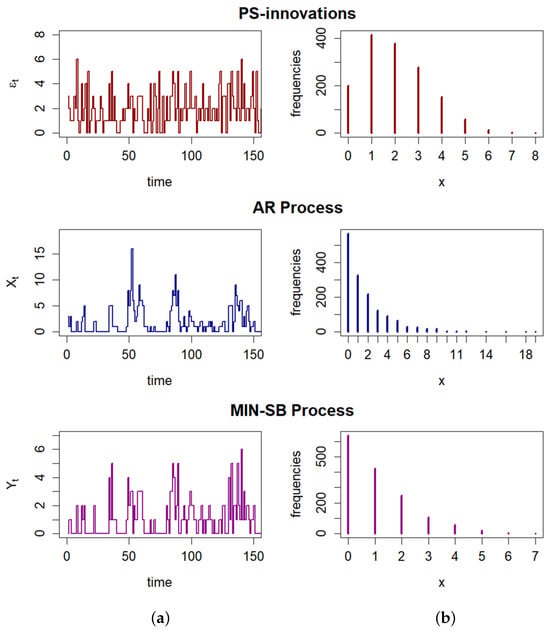
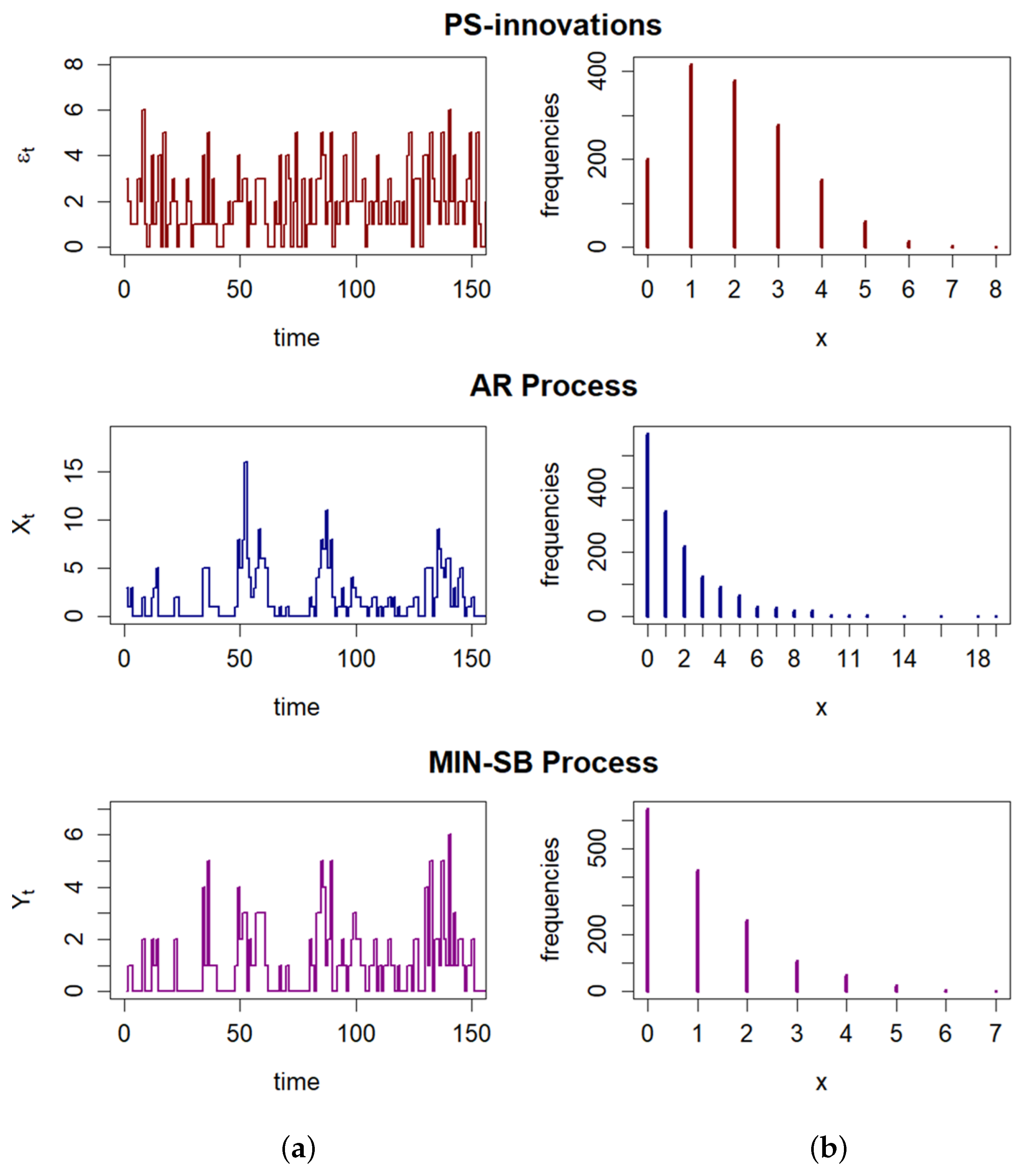
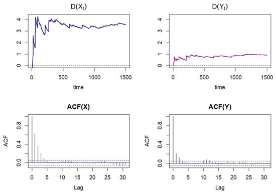
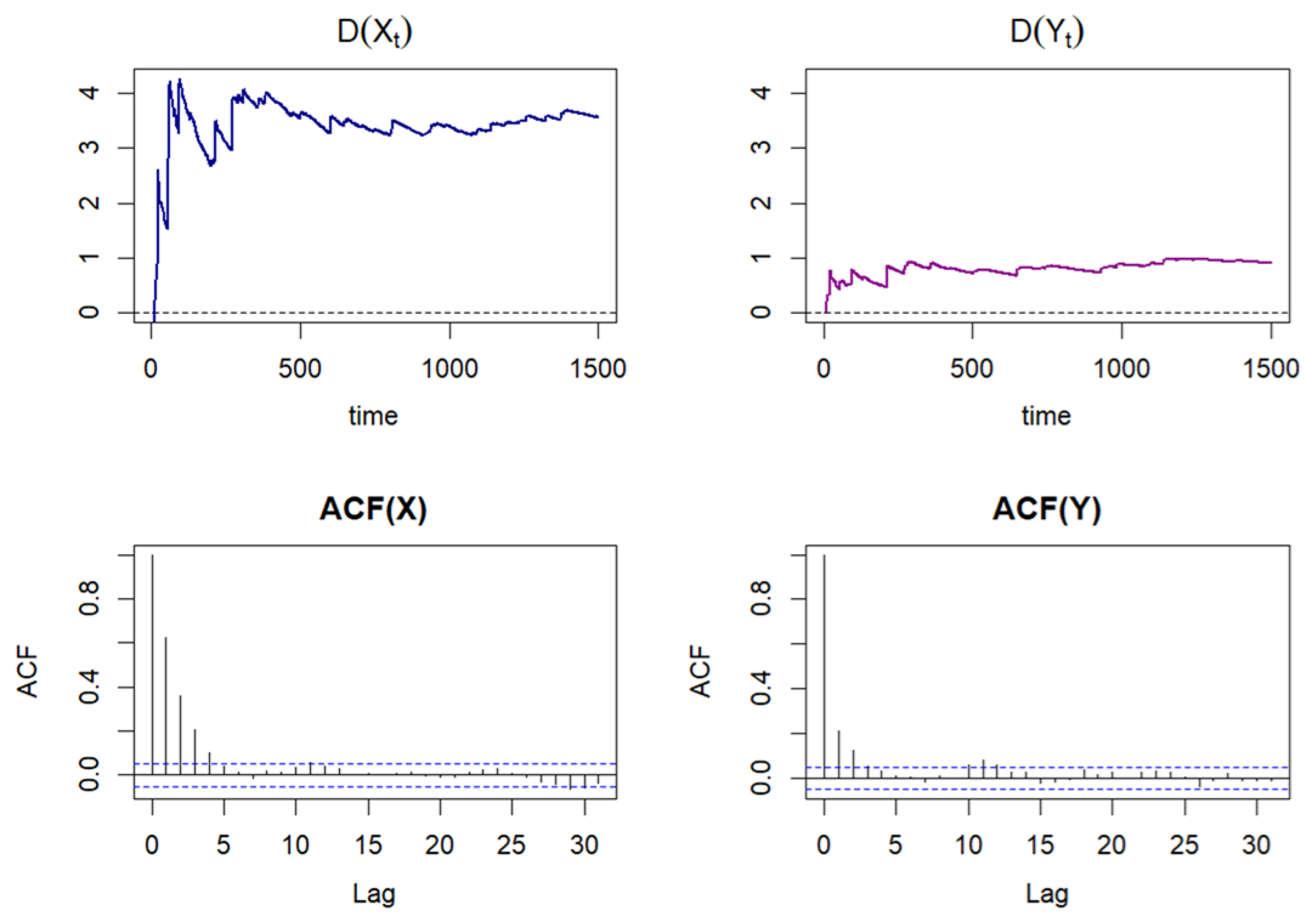
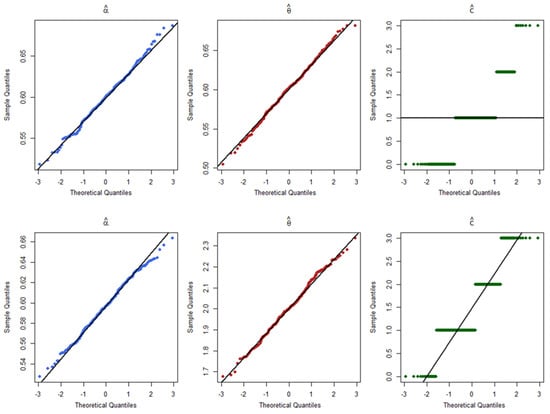
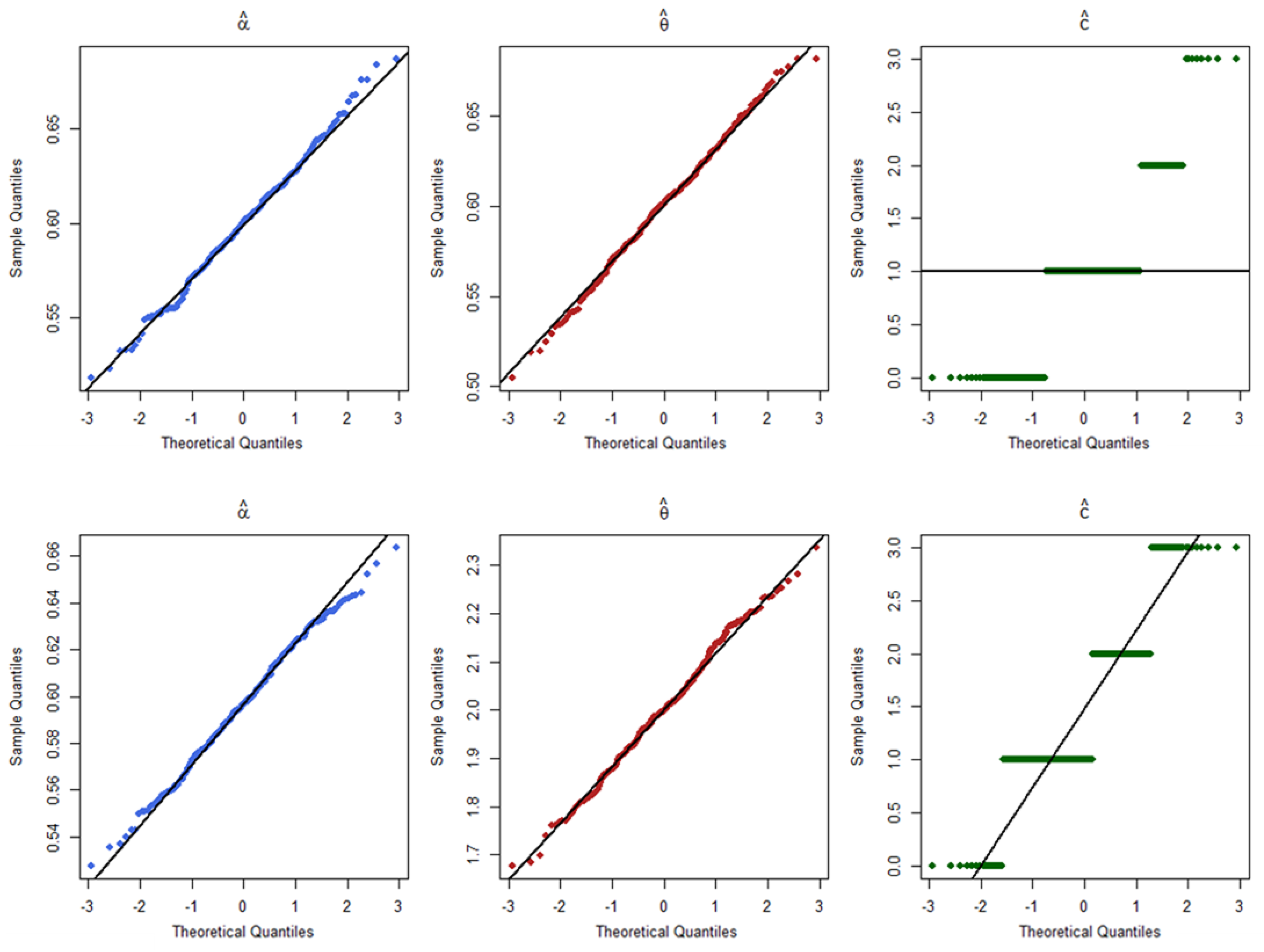
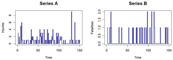
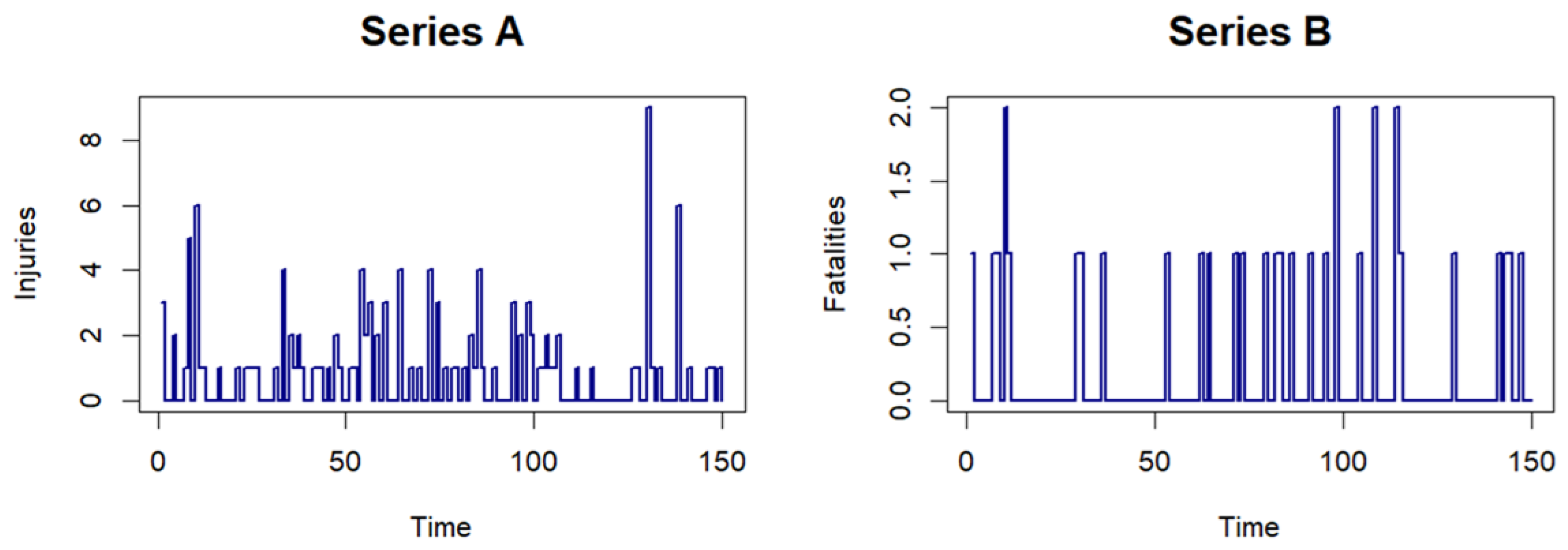
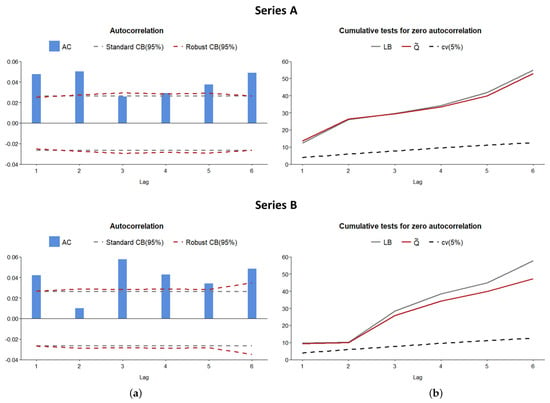
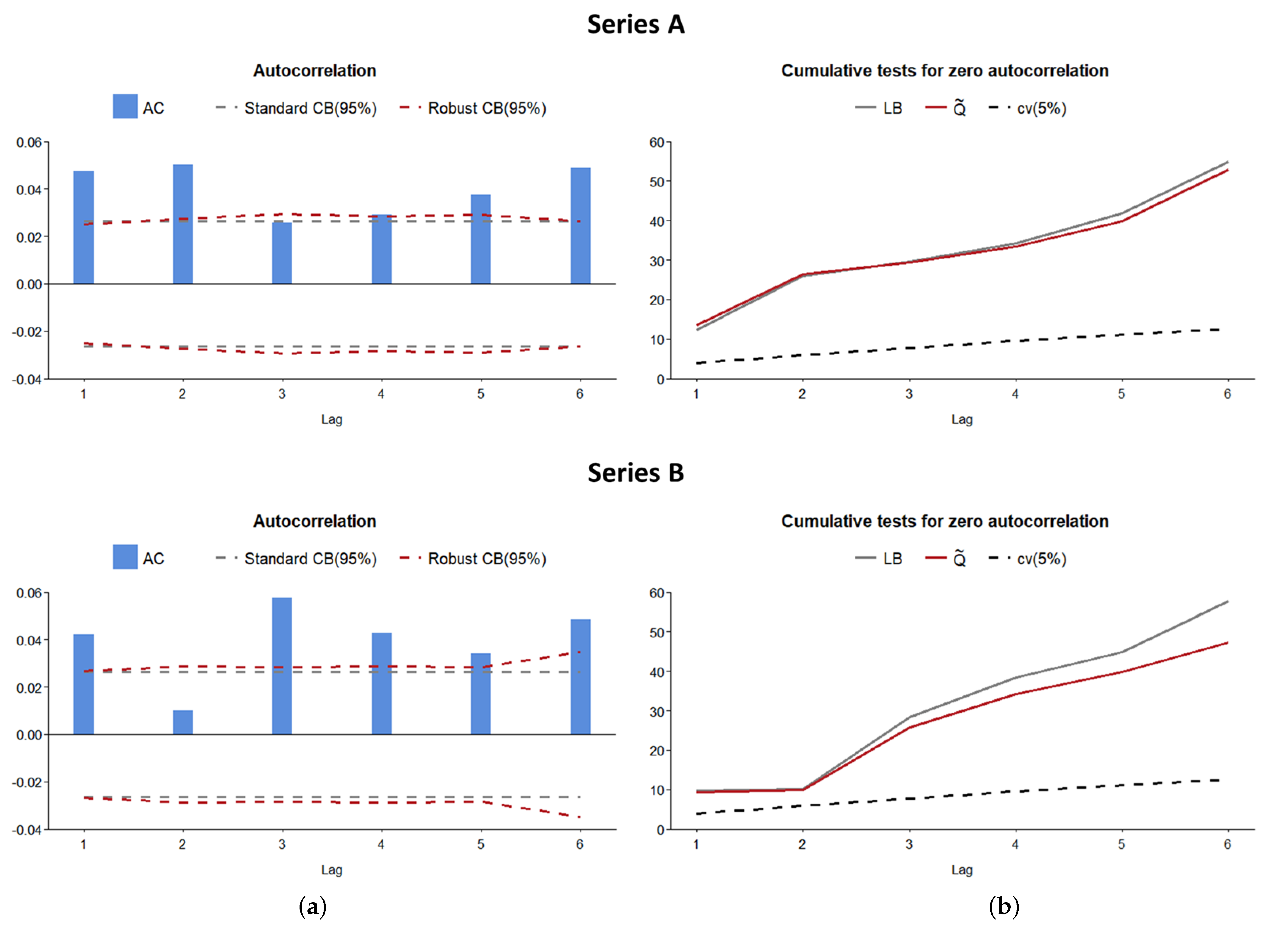
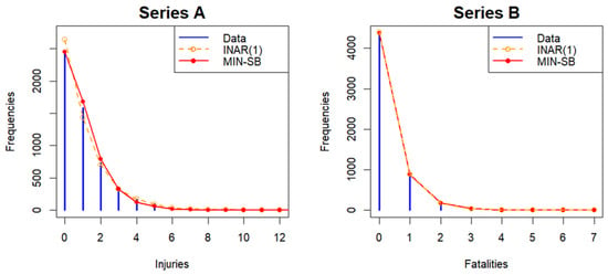
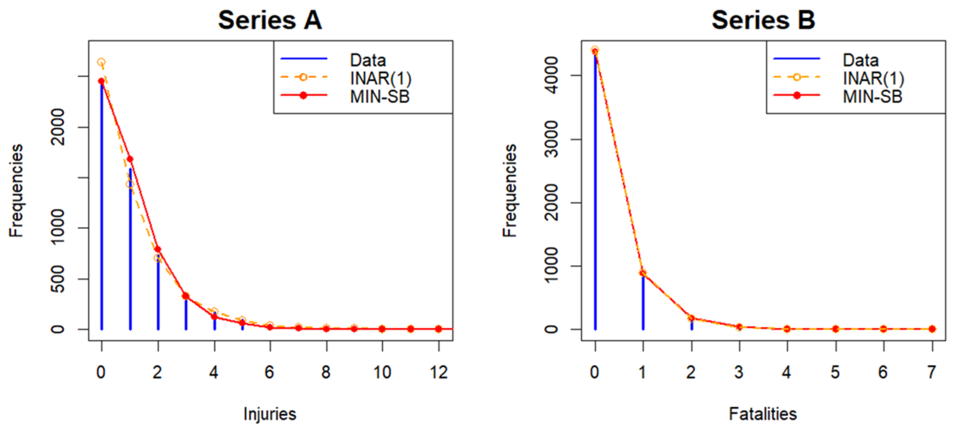

Disclaimer/Publisher’s Note: The statements, opinions and data contained in all publications are solely those of the individual author(s) and contributor(s) and not of MDPI and/or the editor(s). MDPI and/or the editor(s) disclaim responsibility for any injury to people or property resulting from any ideas, methods, instructions or products referred to in the content. |
© 2026 by the authors. Licensee MDPI, Basel, Switzerland. This article is an open access article distributed under the terms and conditions of the Creative Commons Attribution (CC BY) license.