ANN-Assisted Sharp Bounds for Higher-Order Euler–Maclaurin Inequalities

Abstract

This study presents some novel sharp estimates of the Euler–Maclaurin inequality using a new higher-order derivative Maclaurin identity. By utilizing the properties of convexity and classical inequalities, we exploit various novel tight boundaries of the Euler–Maclaurin inequality. They offer alternatives to measuring the sharp bounds of the mean integral of the higher-order differentiable mappings. In order to prove the importance and precision of the key findings, we apply graphical and numerical techniques. Another important section evaluates the behavior and validity of inequalities using a neural network model. The method is not only utilized to authenticate the results but also brings out the practical advancements of the study within a computational framework. The method and results of the article provide an insight and develop a solid connection between inequalities, higher-order derivative convex mappings, numerical analysis, approximation theory, and artificial neural networking.

1. Introduction and Preliminaries

The subject of inequalities is being exploited to approximate various mathematical quantities, and most of the fundamental concepts of mathematical analysis have been created utilizing the premise of inequality. One of them is convex mappings, which are very valuable in identifying significant results such as Hölder-type inequalities, the discrete and integral Jensen inequality, the trapezoidal inequality, and various error inequalities. On the other hand, these fundamental inequalities are discussed as alternatives and featured characterizations of convex mappings in the literature. The benchmark concept of mappings preserving convexity is defined as follows.

Definition 1. 

If $f:[a,b]\to \mathbb{R}$ satisfies the following inequality,

$$\begin{array}{c}\hfill f\left(\right(1-\gamma )x+\gamma y)\le (1-\gamma )f\left(x\right)+\gamma f\left(y\right),\forall x,y\in [a,b],\end{array}$$

(1)

where $\gamma \in [0,1]$, then it is known as a convex mapping.

Theorem 1. 

If $f:I=[a,b]\subset \mathbb{R}\to \mathbb{R}$ is a convex mapping, then

$$\begin{array}{c}\hfill f\left({\displaystyle \frac{a+b}{2}}\right)\le {\displaystyle \frac{1}{\mathcal{l}}}{\int }_a^{b}f\left(\gamma \right)\mathrm{d}\gamma \le {\displaystyle \frac{f\left(a\right)+f\left(b\right)}{2}}.\end{array}$$

(2)

This double inequality has been explored from multiple points of view, and it acts as a base point to develop its general and refined forms due to significant implications. From this result, it can be easily observed that this inequality provides the bounds of definite integrals. Focusing on its left- and right-sided estimation, we can derive the error formulas for mid-point and trapezium rules respectively. This leads us to evaluate the error inequalities of other open and closed schemes, for which a large amount of work has been carried out. For more details regarding Hermite–Hadamard inequalities, consult [1,2].

First, we define the following terms:

• Let $\mathcal{l}=b-a$ represent the length and $x_1={\displaystyle \frac{5a+b}{6}}$, $x_2={\displaystyle \frac{a+b}{2}}$ and $x_3={\displaystyle \frac{a+5b}{6}}$ three points on interval $[a,b]$. Moreover, ${\displaystyle \frac{a-\gamma \mathcal{l}+b}{2}}={\displaystyle \frac{1+\gamma }{2}}a+{\displaystyle \frac{1-\gamma }{2}}b$ and ${\displaystyle \frac{a+\gamma \mathcal{l}+b}{2}}={\displaystyle \frac{1-\gamma }{2}}a+{\displaystyle \frac{1+\gamma }{2}}b$.
• The norm for the n-order differentiable bounded mapping is defined as $\left|\right|f^{\left(n\right)}{\left|\right|}_{\infty }={sup}_{x\in (a,b)}\left|f^{\left(n\right)}\right|<\infty$.
• The space of integrable mappings over $[a,b]$ is represented by $Ł[a,b]$.

Now, we recover the frequently considered three-point numerical integration formula and corresponding error inequality as follows:

$$\begin{array}{c}\hfill {\int }_a^{b}f\left(x\right)\mathrm{d}x={\displaystyle \frac{1}{6}}\left[f\left(a\right)+4f\left(x_2\right)+f\left(b\right)\right]\end{array}$$

Theorem 2 

([3]). If $f:[a,b]\to \mathbb{R}$ is four-time continuously differentiable on $(a,b)$, then

$$\begin{array}{c}\hfill \left|{\displaystyle \frac{1}{6}}\left[f\left(a\right)+4f\left(x_2\right)+f\left(b\right)\right]-{\displaystyle \frac{1}{\mathcal{l}}}{\int }_a^{b}f\left(x\right)\mathrm{d}x\right|\le {\displaystyle \frac{{\left(\mathcal{l}\right)}^5}{2880}}\left|\right|f^{\left(4\right)}{\left|\right|}_{\infty },\end{array}$$

where $\left|\right|f^{\left(n\right)}{\left|\right|}_{\infty }={sup}_{x\in (a,b)}\left|f^{\left(n\right)}\right|<\infty$.

The above-mentioned formulation is only applicable for those mappings that are continuous on endpoints. To tackle such problems, open methods are the primary source, and the three-point open scheme is referred to as Maclaurin’s method. Here, we come up with its error inequality.

$$\begin{array}{cc}\hfill & \left|{\displaystyle \frac{1}{8}}\left(3f\left(x_1\right)+2f\left(x_2\right)+3f\left(x_3\right)\right)-{\displaystyle \frac{1}{\mathcal{l}}}{\int }_a^{b}f\left(x\right)\mathrm{d}x\right|\le {\displaystyle \frac{7{\left(\mathcal{l}\right)}^2}{\mathrm{51,840}}}{\parallel f^{\left(4\right)}\parallel }_{\infty }.\hfill \end{array}$$

In 2009, Alomari et al. [4] utilized s-convexity to investigate the general form of Simpson’s inequalities. In [5], the authors computed some general representations of Simpson’s approximations under $(s,m)$ convex maps. In [6], the authors derived new refinements of the Bullen–Mercer inequality with implications to iterative schemes. Some estimates of the q-Simpson type were discussed in [7]. In [8], various type of inequalities were derived through the applications of equations governed by green mappings and convexity. Working on the sharp composite estimates of Simpson’s rule, various estimates were investigated in [9]. In 2020, Chu et al. [10] introduced a novel class of strong convexity based on n-polynomial and examined significant modifications of Katugampola fractional Simpson-kind inequalities. Alomari and Dragomir worked on a parametric approach to examine various open and closed error approximations of numerical integration techniques, including the open Simpson inequality in [11]. In [12], the authors used extended convexity in fractal space to estimate error inequalities for Maclaurin’s technique. In 2023, Hezenci and his fellow researchers [13] evaluated the fractional variations in error inequality of Maclaurin’s type for convex mappings. In 2013, Latif [14] investigated trapezoid-like inequality relations about higher-order differentiability of preinvex mappings. In [15], the authors constructed bounds utilizing the convexity properties of n-time differentiable mappings. Additionally, Agarwal and his co-authors [16] demonstrated refined estimations using Hölder’s inequality developed by Işcan and using the convexity of the mappings. Qayyum et al. [17] constructed bounds and applications for the numerical analysis of higher-order differentiable mappings. To discuss the convergence analysis of methods, see [18]. For more details, see [19,20].

Today, we are living in the era of artificial intelligence (AI). The tools and techniques evolved under its environment are easily accessible and reduce computational cost. An artificial neural network is among the featured tools of AI having diverse applications in diverse fields including mathematics. It provides new insights to investigate complex mathematical models with great ease. Motivated by the ongoing research, in [21], the authors used an ANN to verify inequalities and the parameter space involved in them.

An ANN learns quickly from datasets and predict estimates. The whole procedure depends on three steps: learning, testing and validation. An ANN can be trained by using the data stemming from a mathematical expression under various parameters. Furthermore, for the solution of differential equations whose solution cannot be assessed by classical methodologies, one can apply deep leaning techniques; for more details, see [22]. Furthermore, the role of PINNs in exploring governing mathematical models is unprecedented; for more information, refer to the following articles [23,24]. In all previous studies, the Euler–Maclaurin method only determined upper bounds of error boundaries for first-order differentiable mappings. We aim to investigate sharp and generalized estimates of Maclaurin’s inequality for higher-order differentiable convex mappings with an artificial neural network analysis. Our study is structured in three segments. We begin by presenting a brief background of the research problem. In the next section, we derive our desired results using a general equation and the convexity property of the mappings. Additionally, we present a few important deductions of principal outcomes along with graphical and tabular illustrations. Next, we develop an artificial neural network to assess the accuracy and sharpness of the inequalities. Finally, we furnish applications of differences of means and special mappings.

2. Fundamental Results

This part of the study offers key results that support our claim. Firstly, we establish a new supporting result that is crucial for the development of our main conclusions.

Lemma 1. 

Let $f:[a,b]\to \mathbb{R}$ be an n-time differentiable mapping over $(a,b)$ and $f^n\in Ł[a,b]$, then

$$\begin{array}{cc}\hfill & {\displaystyle \sum _{k=0}^{n-1}}{\displaystyle \frac{{\left(\mathcal{l}\right)}^k}{(k+1)2^{k+1}}}\left\{\left[{\left({\displaystyle \frac{5}{12}}\right)}^{k+1}+{(-1)}^k{\left({\displaystyle \frac{1}{3}}\right)}^{k+1}\right]f\left(x_1\right)+\left[{\left({\displaystyle \frac{1}{4}}\right)}^{k+1}+{(-1)}^k{\left({\displaystyle \frac{1}{4}}\right)}^{k+1}\right]\times \right.\hfill \\ \hfill & \left.f^k\left(x_2\right)+\left[{\left({\displaystyle \frac{1}{3}}\right)}^{k+1}+{(-1)}^k{\left({\displaystyle \frac{5}{12}}\right)}^{k+1}\right]f^k\left(x_3\right)\right\}-{\displaystyle \frac{1}{\mathcal{l}}}{\int }_a^{b}f\left(u\right)\mathrm{d}u\hfill \\ \hfill & ={\displaystyle \frac{{\left(\mathcal{l}\right)}^n}{{(-1)}^{n+1}{2}^{n+1}n!}}\left[{\int }_0^{{\displaystyle \frac{2}{3}}}{\left(\gamma -{\displaystyle \frac{1}{4}}\right)}^n{f}^n\left({\displaystyle \frac{a+\gamma \mathcal{l}+b}{2}}\right)\mathrm{d}\gamma +{\int }_0^{{\displaystyle \frac{2}{3}}}{\left({\displaystyle \frac{1}{4}}-\gamma \right)}^n{f}^n\left({\displaystyle \frac{a-\gamma \mathcal{l}+b}{2}}\right)\mathrm{d}\gamma \right.\hfill \\ \hfill & \left.+{\int }_{{\displaystyle \frac{2}{3}}}^1{\left(\gamma -1\right)}^n{f}^n\left({\displaystyle \frac{a+\gamma \mathcal{l}+b}{2}}\right)\mathrm{d}\gamma +{\int }_{{\displaystyle \frac{2}{3}}}^1{\left(1-\gamma \right)}^n{f}^n\left({\displaystyle \frac{a-\gamma \mathcal{l}+b}{2}}\right)\mathrm{d}\gamma \right].\hfill \end{array}$$

(3)

Proof. 

By taking (3) into account, we have

$$\begin{array}{cc}\hfill I& ={\displaystyle \frac{{\left(\mathcal{l}\right)}^n}{{(-1)}^{n+1}{2}^{n+1}n!}}\left[{\int }_0^{{\displaystyle \frac{2}{3}}}{\left(\gamma -{\displaystyle \frac{1}{4}}\right)}^n{f}^n\left({\displaystyle \frac{a+\gamma \mathcal{l}+b}{2}}\right)\mathrm{d}\gamma +{\int }_0^{{\displaystyle \frac{2}{3}}}{\left({\displaystyle \frac{1}{4}}-\gamma \right)}^n{f}^n\left({\displaystyle \frac{a-\gamma \mathcal{l}+b}{2}}\right)\mathrm{d}\gamma \right.\hfill \\ \hfill & \left.+{\int }_{{\displaystyle \frac{2}{3}}}^1{\left(\gamma -1\right)}^n{f}^n\left({\displaystyle \frac{a+\gamma \mathcal{l}+b}{2}}\right)\mathrm{d}\gamma +{\int }_{{\displaystyle \frac{2}{3}}}^1{\left(1-\gamma \right)}^n{f}^n\left({\displaystyle \frac{a-\gamma \mathcal{l}+b}{2}}\right)\mathrm{d}\gamma \right]\hfill \\ \hfill & =[I_1+I_2+I_3+I_4].\hfill \end{array}$$

(4)

Integrating by parts, we have

$$\begin{array}{cc}\hfill I_1& ={\int }_0^{{\displaystyle \frac{2}{3}}}{\left(\gamma -{\displaystyle \frac{1}{4}}\right)}^n{f}^n\left({\displaystyle \frac{a+\gamma \mathcal{l}+b}{2}}\right)\mathrm{d}\gamma \hfill \\ \hfill & ={\left.{\displaystyle \frac{2}{\mathcal{l}}}{\left(\gamma -{\displaystyle \frac{1}{4}}\right)}^n{f}^{n-1}\left({\displaystyle \frac{a+\gamma \mathcal{l}+b}{2}}\right)\right|}_0^{{\displaystyle \frac{2}{3}}}-{\displaystyle \frac{2n}{\mathcal{l}}}{\int }_0^{{\displaystyle \frac{2}{3}}}{\left(\gamma -{\displaystyle \frac{1}{4}}\right)}^{n-1}{f}^{n-1}\left({\displaystyle \frac{a+\gamma \mathcal{l}+b}{2}}\right)\mathrm{d}\gamma \hfill \\ \hfill & ={\displaystyle \frac{2}{\mathcal{l}}}{\left({\displaystyle \frac{5}{12}}\right)}^n{f}^{n-1}\left(x_3\right)-{\displaystyle \frac{2}{\mathcal{l}}}{\left(-{\displaystyle \frac{1}{4}}\right)}^n{f}^{n-1}\left(x_2\right)-{\displaystyle \frac{2n}{\mathcal{l}}}{\int }_0^{{\displaystyle \frac{2}{3}}}{\left(\gamma -{\displaystyle \frac{1}{4}}\right)}^{n-1}{f}^{n-1}\left({\displaystyle \frac{a+\gamma \mathcal{l}+b}{2}}\right)\mathrm{d}\gamma \hfill \end{array}$$

Again, applying integration by parts, we get

$$\begin{array}{cc}\hfill & ={\displaystyle \frac{2}{\mathcal{l}}}{\left({\displaystyle \frac{5}{12}}\right)}^n{f}^{n-1}\left(x_3\right)-{\displaystyle \frac{2}{\mathcal{l}}}{\left(-{\displaystyle \frac{1}{4}}\right)}^n{f}^{n-1}\left(x_2\right)-{\displaystyle \frac{2n}{\mathcal{l}}}\left[{\left.{\displaystyle \frac{2}{\mathcal{l}}}{\left(\gamma -{\displaystyle \frac{1}{4}}\right)}^{n-1}{f}^{n-2}\left({\displaystyle \frac{a+\gamma \mathcal{l}+b}{2}}\right)\right|}_0^{{\displaystyle \frac{2}{3}}}\right.\hfill \\ \hfill & \left.-{\displaystyle \frac{2(n-1)}{\mathcal{l}}}{\int }_0^{{\displaystyle \frac{2}{3}}}{\left(\gamma -{\displaystyle \frac{1}{4}}\right)}^{n-2}{f}^{n-2}\left({\displaystyle \frac{a+\gamma \mathcal{l}+b}{2}}\right)\mathrm{d}\gamma \right]\hfill \\ \hfill & ={\displaystyle \frac{2}{\mathcal{l}}}{\left({\displaystyle \frac{5}{12}}\right)}^n{f}^{n-1}\left(x_3\right)-{\displaystyle \frac{2}{\mathcal{l}}}{\left(-{\displaystyle \frac{1}{4}}\right)}^n{f}^{n-1}\left(x_2\right){\displaystyle \frac{2^{2}n}{{\left(\mathcal{l}\right)}^2}}{\left(-{\displaystyle \frac{1}{4}}\right)}^{n-1}{f}^{n-2}\left(x_2\right)\hfill \\ \hfill & -{\displaystyle \frac{2^{2}n(n-1)}{{\left(\mathcal{l}\right)}^2}}{\int }_0^{{\displaystyle \frac{2}{3}}}{\left(\gamma -{\displaystyle \frac{1}{4}}\right)}^{n-2}{f}^{n-2}\left({\displaystyle \frac{a+\gamma \mathcal{l}+b}{2}}\right)\mathrm{d}\gamma .\hfill \end{array}$$

By continuing this process, we get

$$\begin{array}{cc}\hfill I_1& ={\int }_0^{{\displaystyle \frac{2}{3}}}{\left(\gamma -{\displaystyle \frac{1}{4}}\right)}^n{f}^n\left({\displaystyle \frac{a+\gamma \mathcal{l}+b}{2}}\right)\mathrm{d}\gamma \hfill \\ \hfill & ={\displaystyle \sum _{k=0}^{n-1}}{\displaystyle \frac{{(-1)}^{n-k+1}n!2^{n-k}}{(k+1)!{\left(\mathcal{l}\right)}^{n-k}}}{\left({\displaystyle \frac{5}{12}}\right)}^{k+1}{f}^k\left(x_3\right)+{\displaystyle \frac{{(-1)}^{n-k}n!2^{n-k}}{(k+1)!{\left(\mathcal{l}\right)}^{n-k}}}{\left({\displaystyle \frac{-1}{4}}\right)}^{k+1}{f}^k\left(x_2\right)\hfill \\ \hfill & +{\displaystyle \frac{{(-1)}^n{2}^{n}n!}{{\left(\mathcal{l}\right)}^n}}{\int }_0^{{\displaystyle \frac{2}{3}}}f\left({\displaystyle \frac{a+\gamma \mathcal{l}+b}{2}}\right)\mathrm{d}\gamma .\hfill \end{array}$$

(5)

Through a similar process, we gain

$$\begin{array}{cc}\hfill I_2& ={\int }_0^{{\displaystyle \frac{2}{3}}}{\left({\displaystyle \frac{1}{4}}-\gamma \right)}^n{f}^n\left({\displaystyle \frac{a-\gamma \mathcal{l}+b}{2}}\right)\mathrm{d}\gamma \hfill \\ \hfill & ={\displaystyle \sum _{k=0}^{n-1}}{\displaystyle \frac{{(-1)}^{n-k+1}n!2^{n-k}}{(k+1)!{\left(\mathcal{l}\right)}^{n-k}}}{\left({\displaystyle \frac{1}{4}}\right)}^{k+1}{f}^k\left(x_2\right)+{\displaystyle \frac{{(-1)}^{n-k}n!2^{n-k}}{(k+1)!{\left(\mathcal{l}\right)}^{n-k}}}{\left({\displaystyle \frac{-5}{12}}\right)}^{k+1}{f}^k\left(x_1\right)\hfill \\ \hfill & +{\displaystyle \frac{{(-1)}^n{2}^{n}n!}{{\left(\mathcal{l}\right)}^n}}{\int }_0^{{\displaystyle \frac{2}{3}}}f\left({\displaystyle \frac{a-\gamma \mathcal{l}+b}{2}}\right)\mathrm{d}\gamma .\hfill \end{array}$$

(6)

$$\begin{array}{cc}\hfill I_3& ={\int }_{{\displaystyle \frac{2}{3}}}^1{\left(\gamma -1\right)}^n{f}^n\left({\displaystyle \frac{a+\gamma \mathcal{l}+b}{2}}\right)\mathrm{d}\gamma \hfill \\ \hfill & ={\displaystyle \sum _{k=0}^{n-1}}{\displaystyle \frac{{(-1)}^{n-k}n!2^{n-k}}{(k+1)!{\left(\mathcal{l}\right)}^{n-k}}}{\left({\displaystyle \frac{-1}{3}}\right)}^{k+1}{f}^k\left(x_3\right)+{\displaystyle \frac{{(-1)}^n{2}^{n}n!}{{\left(\mathcal{l}\right)}^n}}{\int }_{{\displaystyle \frac{2}{3}}}^{1}f\left({\displaystyle \frac{a+\gamma \mathcal{l}+b}{2}}\right)\mathrm{d}\gamma .\hfill \end{array}$$

(7)

And

$$\begin{array}{cc}\hfill I_4& ={\int }_{{\displaystyle \frac{2}{3}}}^1{\left(1-\gamma \right)}^n{f}^n\left({\displaystyle \frac{a-\gamma \mathcal{l}+b}{2}}\right)\mathrm{d}\gamma \hfill \\ \hfill & ={\displaystyle \sum _{k=0}^{n-1}}{\displaystyle \frac{{(-1)}^{n-k+1}n!2^{n-k}}{(k+1)!{\left(\mathcal{l}\right)}^{n-k}}}{\left({\displaystyle \frac{1}{3}}\right)}^{k+1}{f}^k\left(x_1\right)+{\displaystyle \frac{{(-1)}^n{2}^{n}n!}{{\left(\mathcal{l}\right)}^n}}{\int }_{{\displaystyle \frac{2}{3}}}^{1}f\left({\displaystyle \frac{a-\gamma \mathcal{l}+b}{2}}\right)\mathrm{d}\gamma .\hfill \end{array}$$

(8)

Substituting (5)–(8) in (4), we have

$$\begin{array}{cc}\hfill I& ={\displaystyle \sum _{k=0}^{n-1}}{\displaystyle \frac{{\left(\mathcal{l}\right)}^k}{(k+1)2^{k+1}}}\left\{\left[{\left({\displaystyle \frac{5}{12}}\right)}^{k+1}+{(-1)}^k{\left({\displaystyle \frac{1}{3}}\right)}^{k+1}\right]f\left(x_1\right)+\left[{\left({\displaystyle \frac{1}{4}}\right)}^{k+1}+{(-1)}^k{\left({\displaystyle \frac{1}{4}}\right)}^{k+1}\right]f^k\left(x_2\right)\right.\hfill \\ \hfill & \left.+\left[{\left({\displaystyle \frac{1}{3}}\right)}^{k+1}+{(-1)}^k{\left({\displaystyle \frac{5}{12}}\right)}^{k+1}\right]f^k\left(x_3\right)\right\}\hfill \\ \hfill & +{\displaystyle \frac{1}{2}}{\int }_0^1\left[f\left({\displaystyle \frac{a+\gamma \mathcal{l}+b}{2}}\right)+f\left({\displaystyle \frac{a-\gamma \mathcal{l}+b}{2}}\right)\right]\mathrm{d}\gamma .\hfill \end{array}$$

By applying the technique of substitution, we acquire our desired left-hand side of (3).    □

2.1. Sharp Bounds of Euler–Maclaurin Inequality

Now, we present new error bounds for Euler–Maclaurin’s inequality utilizing the convexity of the mappings.

Theorem 3. 

Assume that $f:[a,b]\to$ is an nth-order differentiable mapping and $|f^n{|}^{\mathfrak{q}}$ is convex with $q\ge 1$. If $|f^n{|}^q\in Ł[a,b]$, then

$$\begin{array}{cc}\hfill & \left|{\displaystyle \sum _{k=0}^{n-1}}{\displaystyle \frac{{\left(\mathcal{l}\right)}^k}{(k+1)2^{k+1}}}\left\{\left[{\left({\displaystyle \frac{5}{12}}\right)}^{k+1}+{(-1)}^k{\left({\displaystyle \frac{1}{3}}\right)}^{k+1}\right]f^k\left(x_1\right)+\left[{\left({\displaystyle \frac{1}{4}}\right)}^{k+1}+{(-1)}^k{\left({\displaystyle \frac{1}{4}}\right)}^{k+1}\right]\times \right.\right.\hfill \\ & \left.\left.f^k\left(x_2\right)+\left[{\left({\displaystyle \frac{1}{3}}\right)}^{k+1}+{(-1)}^k{\left({\displaystyle \frac{5}{12}}\right)}^{k+1}\right]f^k\left(x_3\right)\right\}-{\displaystyle \frac{1}{\mathcal{l}}}{\int }_a^{b}f\left(u\right)\mathrm{d}u\right|\hfill \\ \hfill & \le {\displaystyle \frac{{\left(\mathcal{l}\right)}^n}{2^{n+1}n!}}\left[{\left({\displaystyle \frac{3^{n+1}+5^{n+1}}{{12}^{n+1}(n+1)}}\right)}^{1-{\displaystyle \frac{1}{\mathfrak{q}}}}((D_1|f^n{\left(a\right)|}^{\mathfrak{q}}+D_2|f^n{\left(b\right)|}^{\mathfrak{q}}{)}^{{\displaystyle \frac{1}{\mathfrak{q}}}}+(D_2|f^n{\left(a\right)|}^{\mathfrak{q}}+D_1|f^n\left(b\right){{|}^{\mathfrak{q}})}^{{\displaystyle \frac{1}{\mathfrak{q}}}})\right.\hfill \\ \hfill & \left.+{\left({\displaystyle \frac{3^{-n-1}}{n+1}}\right)}^{1-{\displaystyle \frac{1}{\mathfrak{q}}}}((D_3|f^n{\left(a\right)|}^{\mathfrak{q}}+D_4|f^n{\left(b\right)|}^{\mathfrak{q}}{)}^{{\displaystyle \frac{1}{\mathfrak{q}}}}+(D_4|f^n{\left(a\right)|}^{\mathfrak{q}}+D_3|f^n\left(b\right){{|}^{\mathfrak{q}})}^{{\displaystyle \frac{1}{\mathfrak{q}}}})\right].\hfill \end{array}$$

(9)

$$\begin{array}{cc}\hfill D_1& ={\int }_0^{{\displaystyle \frac{2}{3}}}{\left|\gamma -{\displaystyle \frac{1}{4}}\right|}^n\left({\displaystyle \frac{1-\gamma }{2}}\right)\mathrm{d}\gamma \hfill \\ \hfill & ={\int }_0^{{\displaystyle \frac{1}{4}}}{\left({\displaystyle \frac{1}{4}}-\gamma \right)}^n\left({\displaystyle \frac{1-\gamma }{2}}\right)\mathrm{d}\gamma +{\int }_{{\displaystyle \frac{1}{4}}}^{{\displaystyle \frac{2}{3}}}{\left(\gamma -{\displaystyle \frac{1}{4}}\right)}^n\left({\displaystyle \frac{1-\gamma }{2}}\right)\mathrm{d}\gamma \hfill \\ \hfill & ={\displaystyle \frac{\left(4n\left(3^{n+2}+5^{n+1}\right)+13\times 5^{n+1}+7\times 3^{n+2}\right)}{2^{2n+5}{3}^{n+2}(n+1)(n+2)}}\hfill \\ \hfill & D_2={\int }_0^{{\displaystyle \frac{2}{3}}}{\left|\gamma -{\displaystyle \frac{1}{4}}\right|}^n\left({\displaystyle \frac{1+\gamma }{2}}\right)\mathrm{d}\gamma ={\displaystyle \frac{\left(4n\left(3^{n+2}+5^{n+2}\right)+7\times 5^{n+2}+3^{n+4}\right)}{2^{2n+5}{3}^{n+2}(n+1)(n+2)}}\hfill \\ \hfill & D_3={\int }_{{\displaystyle \frac{2}{3}}}^1{\left|1-\gamma \right|}^n\left({\displaystyle \frac{1-\gamma }{2}}\right)\mathrm{d}\gamma ={\displaystyle \frac{3^{-n-2}}{2n+4}}\hfill \\ \hfill & D_4={\int }_{{\displaystyle \frac{2}{3}}}^1{\left|1-\gamma \right|}^n\left({\displaystyle \frac{1+\gamma }{2}}\right)\mathrm{d}\gamma ={\displaystyle \frac{3^{-n-2}(5n+11)}{2(n+1)(n+2)}}.\hfill \end{array}$$

Proof. 

Considering Equation (3) and using the convexity of $|f^n{|}^{\mathfrak{q}}$, we attain

$$\begin{array}{cc}\hfill & \left|{\displaystyle \sum _{k=0}^{n-1}}{\displaystyle \frac{{\left(\mathcal{l}\right)}^k}{(k+1)2^{k+1}}}\left\{\left[{\left({\displaystyle \frac{5}{12}}\right)}^{k+1}+{(-1)}^k{\left({\displaystyle \frac{1}{3}}\right)}^{k+1}\right]f^k\left(x_1\right)+\left[{\left({\displaystyle \frac{1}{4}}\right)}^{k+1}+{(-1)}^k{\left({\displaystyle \frac{1}{4}}\right)}^{k+1}\right]\times \right.\right.\hfill \\ & \left.\left.f^k\left(x_2\right)+\left[{\left({\displaystyle \frac{1}{3}}\right)}^{k+1}+{(-1)}^k{\left({\displaystyle \frac{5}{12}}\right)}^{k+1}\right]f^k\left(x_3\right)\right\}-{\displaystyle \frac{1}{\mathcal{l}}}{\int }_a^{b}f\left(u\right)\mathrm{d}u\right|\hfill \\ \hfill & \le {\displaystyle \frac{{\left(\mathcal{l}\right)}^n}{2^{n+1}n!}}\left[{\int }_0^{{\displaystyle \frac{2}{3}}}{\left|\gamma -{\displaystyle \frac{1}{4}}\right|}^n\left|f^n\left({\displaystyle \frac{a+\gamma \mathcal{l}+b}{2}}\right)\right|\mathrm{d}\gamma +{\int }_0^{{\displaystyle \frac{2}{3}}}{\left|{\displaystyle \frac{1}{4}}-\gamma \right|}^n\left|f^n\left({\displaystyle \frac{a-\gamma \mathcal{l}+b}{2}}\right)\right|\mathrm{d}\gamma \right.\hfill \\ \hfill & \left.+{\int }_{{\displaystyle \frac{2}{3}}}^1{\left|\gamma -1\right|}^n\left|f^n\left({\displaystyle \frac{a+\gamma \mathcal{l}+b}{2}}\right)\right|\mathrm{d}\gamma +{\int }_{{\displaystyle \frac{2}{3}}}^1{\left|1-\gamma \right|}^n\left|f^n\left({\displaystyle \frac{a-\gamma \mathcal{l}+b}{2}}\right)\right|\mathrm{d}\gamma \right]\hfill \\ \hfill & \le {\displaystyle \frac{{\left(\mathcal{l}\right)}^n}{2^{n+1}n!}}\left[{\left({\int }_0^{{\displaystyle \frac{2}{3}}}{\left|\gamma -{\displaystyle \frac{1}{4}}\right|}^n\mathrm{d}\gamma \right)}^{1-{\displaystyle \frac{1}{\mathfrak{q}}}}{\left({\int }_0^{{\displaystyle \frac{2}{3}}}{\left|\gamma -{\displaystyle \frac{1}{4}}\right|}^n{\left|f^n\left({\displaystyle \frac{a+\gamma \mathcal{l}+b}{2}}\right)\right|}^{\mathfrak{q}}\mathrm{d}\gamma \right)}^{{\displaystyle \frac{1}{\mathfrak{q}}}}\right.\hfill \\ \hfill & +{\left({\int }_0^{{\displaystyle \frac{2}{3}}}{\left|\gamma -{\displaystyle \frac{1}{4}}\right|}^n\mathrm{d}\gamma \right)}^{1-{\displaystyle \frac{1}{\mathfrak{q}}}}{\left({\int }_0^{{\displaystyle \frac{2}{3}}}{\left|\gamma -{\displaystyle \frac{1}{4}}\right|}^n{\left|f^n\left({\displaystyle \frac{a-\gamma \mathcal{l}+b}{2}}\right)\right|}^{\mathfrak{q}}\mathrm{d}\gamma \right)}^{{\displaystyle \frac{1}{\mathfrak{q}}}}\hfill \\ \hfill & +{\left({\int }_{{\displaystyle \frac{2}{3}}}^1{|1-\gamma |}^n\right)}^{1-{\displaystyle \frac{1}{\mathfrak{q}}}}{\left({\int }_{{\displaystyle \frac{2}{3}}}^1{\left|\gamma -1\right|}^n{\left|f^n\left({\displaystyle \frac{a+\gamma \mathcal{l}+b}{2}}\right)\right|}^{\mathfrak{q}}\mathrm{d}\gamma \right)}^{{\displaystyle \frac{1}{\mathfrak{q}}}}\hfill \\ \hfill & \left.+{\left({\int }_{{\displaystyle \frac{2}{3}}}^1{|1-\gamma |}^n\right)}^{1-{\displaystyle \frac{1}{\mathfrak{q}}}}{\left({\int }_{{\displaystyle \frac{2}{3}}}^1{\left|1-\gamma \right|}^n{\left|f^n\left({\displaystyle \frac{a-\gamma \mathcal{l}+b}{2}}\right)\right|}^{\mathfrak{q}}\mathrm{d}\gamma \right)}^{{\displaystyle \frac{1}{\mathfrak{q}}}}\right]\hfill \\ \hfill & \le {\displaystyle \frac{{\left(\mathcal{l}\right)}^n}{2^{n+1}n!}}\left[{\left({\int }_0^{{\displaystyle \frac{2}{3}}}{\left|\gamma -{\displaystyle \frac{1}{4}}\right|}^n\mathrm{d}\gamma \right)}^{1-{\displaystyle \frac{1}{\mathfrak{q}}}}\left\{{\left({\int }_0^{{\displaystyle \frac{2}{3}}}{\left|\gamma -{\displaystyle \frac{1}{4}}\right|}^n\left({\displaystyle \frac{1-\gamma }{2}}|f^n{\left(a\right)|}^{\mathfrak{q}}+{\displaystyle \frac{1+\gamma }{2}}{\left|f^n\left(b\right)\right|}^{\mathfrak{q}}\right)\mathrm{d}\gamma \right)}^{{\displaystyle \frac{1}{\mathfrak{q}}}}\right.\right.\hfill \\ \hfill & \left.+{\left({\int }_0^{{\displaystyle \frac{2}{3}}}{\left|\gamma -{\displaystyle \frac{1}{4}}\right|}^n\left({\displaystyle \frac{1+\gamma }{2}}|f^n{\left(a\right)|}^{\mathfrak{q}}+{\displaystyle \frac{1-\gamma }{2}}{\left|f^n\left(b\right)\right|}^{\mathfrak{q}}\right)\mathrm{d}\gamma \right)}^{{\displaystyle \frac{1}{\mathfrak{q}}}}\right\}\hfill \\ \hfill & +{\left({\int }_{{\displaystyle \frac{2}{3}}}^1{|1-\gamma |}^n\right)}^{1-{\displaystyle \frac{1}{\mathfrak{q}}}}\left\{{\left({\int }_{{\displaystyle \frac{2}{3}}}^1{|1-\gamma |}^n\left({\displaystyle \frac{1-\gamma }{2}}|f^n{\left(a\right)|}^{\mathfrak{q}}+{\displaystyle \frac{1+\gamma }{2}}{\left|f^n\left(b\right)\right|}^{\mathfrak{q}}\right)\mathrm{d}\gamma \right)}^{{\displaystyle \frac{1}{\mathfrak{q}}}}\right.\hfill \\ \hfill & \left.\left.+{\left({\int }_{{\displaystyle \frac{2}{3}}}^1{|1-\gamma |}^n\left({\displaystyle \frac{1+\gamma }{2}}|f^n{\left(a\right)|}^{\mathfrak{q}}+{\displaystyle \frac{1-\gamma }{2}}{\left|f^n\left(b\right)\right|}^{\mathfrak{q}}\right)\mathrm{d}\gamma \right)}^{{\displaystyle \frac{1}{\mathfrak{q}}}}\right\}\right].\hfill \end{array}$$

By computing the aforementioned integrals, we achieve our desired result.    □

Remark 1. 

The inequality (9) proved in Theorem 3 is sharp for $f\left(\varrho \right)={\varrho }^3$ for $q=1$ and $n=2$ over $[0,2]$.

Corollary 1. 

For $\mathfrak{q}=1$, we acquire the following inequality

$$\begin{array}{cc}\hfill & \left|{\displaystyle \sum _{k=0}^{n-1}}{\displaystyle \frac{{\left(\mathcal{l}\right)}^k}{(k+1)2^{k+1}}}\left\{\left[{\left({\displaystyle \frac{5}{12}}\right)}^{k+1}+{(-1)}^k{\left({\displaystyle \frac{1}{3}}\right)}^{k+1}\right]f^k\left(x_1\right)+\left[{\left({\displaystyle \frac{1}{4}}\right)}^{k+1}+{(-1)}^k{\left({\displaystyle \frac{1}{4}}\right)}^{k+1}\right]\times \right.\right.\hfill \\ \hfill & \left.\left.f^k\left(x_2\right)+\left[{\left({\displaystyle \frac{1}{3}}\right)}^{k+1}+{(-1)}^k{\left({\displaystyle \frac{5}{12}}\right)}^{k+1}\right]f^k\left(x_3\right)\right\}-{\displaystyle \frac{1}{\mathcal{l}}}{\int }_a^{b}f\left(u\right)\mathrm{d}u\right|\hfill \\ \hfill & \le {\displaystyle \frac{\left(3^{n+1}+4^{n+1}+5^{n+1}\right){\left(\mathcal{l}\right)}^n}{{24}^{n+1}(n+1)!}}\left[|f^n\left(a\right)|+|f^n\left(b\right)|\right].\hfill \end{array}$$

Corollary 2. 

Setting $n=1$ in Theorem 3, we obtain

$$\begin{array}{cc}\hfill & \left|{\displaystyle \frac{1}{8}}\left[3f\left(x_1\right)+2f\left(x_2\right)+3f\left(x_3\right)\right]-{\displaystyle \frac{1}{\mathcal{l}}}{\int }_a^{b}f\left(x\right)\mathrm{d}x\right|\hfill \\ \hfill & \le {\displaystyle \frac{\left(\mathcal{l}\right)}{4}}\left[{\left({\displaystyle \frac{17}{144}}\right)}^{1-{\displaystyle \frac{1}{\mathfrak{q}}}}\left({\left({\displaystyle \frac{361}{10,368}}|f^{\prime }{\left(a\right)|}^{\mathfrak{q}}+{\displaystyle \frac{863}{10,368}}{\left|f^{\prime }\left(b\right)\right|}^{\mathfrak{q}}\right)}^{{\displaystyle \frac{1}{\mathfrak{q}}}}+{\left({\displaystyle \frac{863}{10,368}}|f^{\prime }{\left(a\right)|}^{\mathfrak{q}}+{\displaystyle \frac{361}{10,368}}{\left|f^{\prime }\left(b\right)\right|}^{\mathfrak{q}}\right)}^{{\displaystyle \frac{1}{\mathfrak{q}}}}\right)\right.\hfill \\ \hfill & \left.+{\left({\displaystyle \frac{1}{18}}\right)}^{1-{\displaystyle \frac{1}{\mathfrak{q}}}}\left({\left({\displaystyle \frac{1}{162}}|f^{\prime }{\left(a\right)|}^{\mathfrak{q}}+{\displaystyle \frac{4}{81}}{\left|f^{\prime }\left(b\right)\right|}^{\mathfrak{q}}\right)}^{{\displaystyle \frac{1}{\mathfrak{q}}}}+{\left({\displaystyle \frac{4}{81}}|f^{\prime }{\left(a\right)|}^{\mathfrak{q}}+{\displaystyle \frac{1}{162}}{\left|f^{\prime }\left(b\right)\right|}^{\mathfrak{q}}\right)}^{{\displaystyle \frac{1}{\mathfrak{q}}}}\right)\right].\hfill \end{array}$$

Now, we deliver the explanation of Theorem 3 in terms of mean value integral by taking the means of $f\left(x\right)={\displaystyle \frac{{\kappa }_1}{{\tau }_1+2{\kappa }_1}}{x}^{{\displaystyle \frac{{\tau }_1}{{\kappa }_1}}+2},{\tau }_1\ge 1$, ${\kappa }_1>1,\mathfrak{q}=2,n=1$ and $[a,b]=[0,6]$.

$$\begin{array}{cc}\hfill T_1& ={\displaystyle \frac{{\kappa }_1\left[3\left(5^{\frac{2{\kappa }_1+{\tau }_1}{{\kappa }_1}}\right)+2\left(3^{\frac{2{\kappa }_1+{\tau }_1}{{\kappa }_1}}\right)+3\right]}{8(2{\kappa }_1+{\tau }_1)}}\hfill \\ \hfill & -{\displaystyle \frac{1}{4}}\left(\left(\sqrt{{\displaystyle \frac{4}{81}}}+\sqrt{{\displaystyle \frac{1}{162}}}\right)\sqrt{{\displaystyle \frac{1}{18}}}+\sqrt{{\displaystyle \frac{17}{144}}}\left(\sqrt{{\displaystyle \frac{361}{10,368}}}+\sqrt{{\displaystyle \frac{863}{10,368}}}\right)\right)6^{{\displaystyle \frac{2{\kappa }_1+{\tau }_1}{{\kappa }_1}}}.\hfill \end{array}$$

$$\begin{array}{c}\hfill T_2={\displaystyle \frac{{{\kappa }_1}^2\left(6^{\frac{2{\kappa }_1+{\tau }_1}{{\kappa }_1}}\right)}{({\tau }_1+2{\kappa }_1)({\tau }_1+3{\kappa }_1)}}.\end{array}$$

$$\begin{array}{cc}\hfill T_3& ={\displaystyle \frac{{\kappa }_1\left[3\left(5^{\frac{2{\kappa }_1+{\tau }_1}{{\kappa }_1}}\right)+2\left(3^{\frac{2{\kappa }_1+{\tau }_1}{{\kappa }_1}}\right)+3\right]}{8(2{\kappa }_1+{\tau }_1)}}+{\displaystyle \frac{1}{16}}\hfill \\ \hfill & +{\displaystyle \frac{1}{4}}\left(\left(\sqrt{{\displaystyle \frac{4}{81}}}+\sqrt{{\displaystyle \frac{1}{162}}}\right)\sqrt{{\displaystyle \frac{1}{18}}}+\sqrt{{\displaystyle \frac{17}{144}}}\left(\sqrt{{\displaystyle \frac{361}{10,368}}}+\sqrt{{\displaystyle \frac{863}{10,368}}}\right)\right)6^{{\displaystyle \frac{2{\kappa }_1+{\tau }_1}{{\kappa }_1}}}.\hfill \end{array}$$

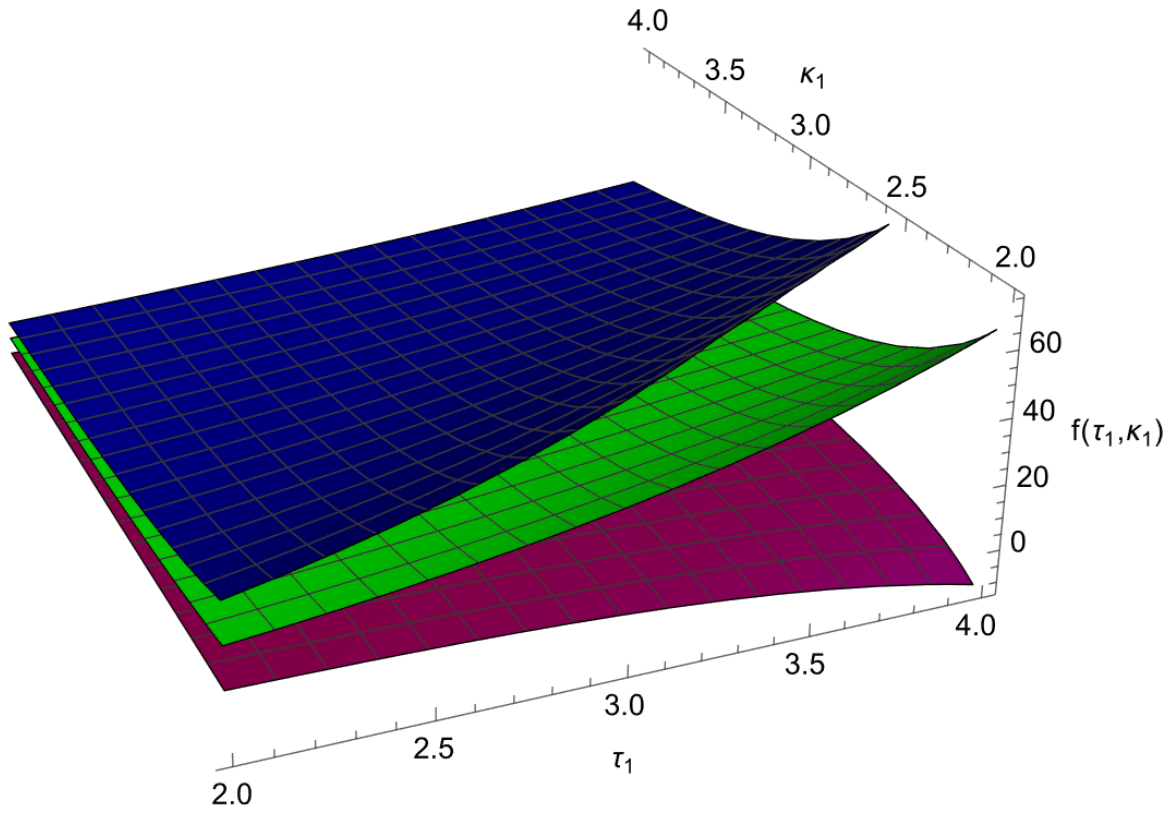
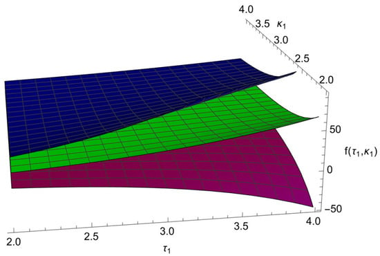
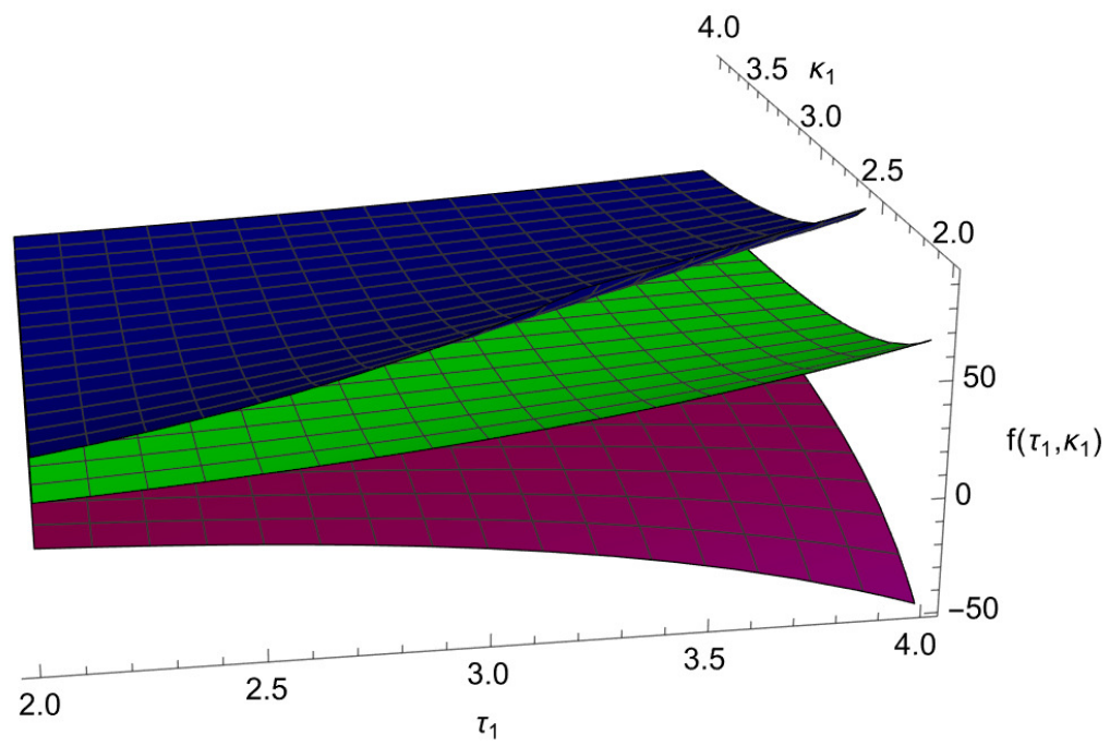
Figure 1 illustrates the accuracy of the mean value integral and its bounds by keeping ${\tau }_1,{\kappa }_1\in [2,4]$ as unknowns. Here, we provide the tabular explanation of the above expressions.

Figure 1. Graphical explanation of Theorem 3.

Table 1 presents the bounds of the average integral through the variation in ${\kappa }_1$. We obtain sharp bounds for larger values of ${\kappa }_1$.

Table 1. Numerical comparison of Theorem 3.

$({\mathit{\tau }}_1,{\mathit{\kappa }}_1)$	${\mathit{T}}_1$	${\mathit{T}}_2$	${\mathit{T}}_3$
$(2,2)$	$5.35$	18	$30.64$
$(2,3)$	$5.21$	$12.1571$	$19.13$
$(2,4)$	$4.93$	$10.0779$	$15.25$
$(2,5)$	$4.73$	$9.03385$	$13.36$
$(2,6)$	$4.59$	$8.41067$	$12.25$
$(2,7)$	$4.49$	$7.99797$	$11.52$
$(2,8)$	$4.41$	$7.70503$	$11.01$

Theorem 4. 

Assume that $f:[a,b]\to$ is an nth-order differentiable mapping and $|f^n{|}^{\mathfrak{q}}$ is convex. If $|f^n{|}^{\mathfrak{q}}\in Ł[a,b]$, then

$$\begin{array}{cc}\hfill & \left|{\displaystyle \sum _{k=0}^{n-1}}{\displaystyle \frac{{\left(\mathcal{l}\right)}^k}{(k+1)2^{k+1}}}\left\{\left[{\left({\displaystyle \frac{5}{12}}\right)}^{k+1}+{(-1)}^k{\left({\displaystyle \frac{1}{3}}\right)}^{k+1}\right]f^k\left(x_1\right)+\left[{\left({\displaystyle \frac{1}{4}}\right)}^{k+1}+{(-1)}^k{\left({\displaystyle \frac{1}{4}}\right)}^{k+1}\right]\times \right.\right.\hfill \\ & \left.\left.f^k\left(x_2\right)+\left[{\left({\displaystyle \frac{1}{3}}\right)}^{k+1}+{(-1)}^k{\left({\displaystyle \frac{5}{12}}\right)}^{k+1}\right]f^k\left(x_3\right)\right\}-{\displaystyle \frac{1}{\mathcal{l}}}{\int }_a^{b}f\left(u\right)\mathrm{d}u\right|\hfill \\ \hfill & \le {\displaystyle \frac{{\left(\mathcal{l}\right)}^n}{2^{n+1}n!}}\left[{\left({\displaystyle \frac{{\left(\frac{12}{5}\right)}^{-np-1}+4^{-np-1}}{np+1}}\right)}^{{\displaystyle \frac{1}{p}}}\left({\left({\displaystyle \frac{2|f^n{\left(a\right)|}^{\mathfrak{q}}+4{\left|f^n\left(b\right)\right|}^{\mathfrak{q}}}{9}}\right)}^{{\displaystyle \frac{1}{\mathfrak{q}}}}+{\left({\displaystyle \frac{4|f^n{\left(a\right)|}^{\mathfrak{q}}+2{\left|f^n\left(b\right)\right|}^{\mathfrak{q}}}{9}}\right)}^{{\displaystyle \frac{1}{\mathfrak{q}}}}\right)\right.\hfill \\ \hfill & \left.+{\left({\displaystyle \frac{3^{-np-1}}{np+1}}\right)}^{{\displaystyle \frac{1}{p}}}\left({\left({\displaystyle \frac{|f^n{\left(a\right)|}^{\mathfrak{q}}+11{\left|f^n\left(b\right)\right|}^{\mathfrak{q}}}{36}}\right)}^{{\displaystyle \frac{1}{\mathfrak{q}}}}+{\left({\displaystyle \frac{11|f^n{\left(a\right)|}^{\mathfrak{q}}+{\left|f^n\left(b\right)\right|}^{\mathfrak{q}}}{36}}\right)}^{{\displaystyle \frac{1}{\mathfrak{q}}}}\right)\right].\hfill \end{array}$$

Proof. 

Considering equation (3), using Hölder’s inequality and the convexity property of $|f^n{|}^{\mathfrak{q}}$, we attain

$$\begin{array}{cc}\hfill & \left|{\displaystyle \sum _{k=0}^{n-1}}{\displaystyle \frac{{\left(\mathcal{l}\right)}^k}{(k+1)2^{k+1}}}\left\{\left[{\left({\displaystyle \frac{5}{12}}\right)}^{k+1}+{(-1)}^k{\left({\displaystyle \frac{1}{3}}\right)}^{k+1}\right]f^k\left(x_1\right)+\left[{\left({\displaystyle \frac{1}{4}}\right)}^{k+1}+{(-1)}^k{\left({\displaystyle \frac{1}{4}}\right)}^{k+1}\right]\times \right.\right.\hfill \\ & \left.\left.f^k\left(x_2\right)+\left[{\left({\displaystyle \frac{1}{3}}\right)}^{k+1}+{(-1)}^k{\left({\displaystyle \frac{5}{12}}\right)}^{k+1}\right]f^k\left(x_3\right)\right\}-{\displaystyle \frac{1}{\mathcal{l}}}{\int }_a^{b}f\left(u\right)\mathrm{d}u\right|\hfill \\ \hfill & \le {\displaystyle \frac{{\left(\mathcal{l}\right)}^n}{2^{n+1}n!}}\left[{\int }_0^{{\displaystyle \frac{2}{3}}}{\left|\gamma -{\displaystyle \frac{1}{4}}\right|}^n\left|f^n\left({\displaystyle \frac{a+\gamma \mathcal{l}+b}{2}}\right)\right|\mathrm{d}\gamma +{\int }_0^{{\displaystyle \frac{2}{3}}}{\left|{\displaystyle \frac{1}{4}}-\gamma \right|}^n\left|f^n\left({\displaystyle \frac{a-\gamma \mathcal{l}+b}{2}}\right)\right|\mathrm{d}\gamma \right.\hfill \\ \hfill & \left.+{\int }_{{\displaystyle \frac{2}{3}}}^1{\left|\gamma -1\right|}^n\left|f^n\left({\displaystyle \frac{a+\gamma \mathcal{l}+b}{2}}\right)\right|\mathrm{d}\gamma +{\int }_{{\displaystyle \frac{2}{3}}}^1{\left|1-\gamma \right|}^n\left|f^n\left({\displaystyle \frac{a-\gamma \mathcal{l}+b}{2}}\right)\right|\mathrm{d}\gamma \right]\hfill \\ \hfill & \le {\displaystyle \frac{{\left(\mathcal{l}\right)}^n}{2^{n+1}n!}}\left[{\left({\int }_0^{{\displaystyle \frac{2}{3}}}{\left|\gamma -{\displaystyle \frac{1}{4}}\right|}^{np}\mathrm{d}\gamma \right)}^{{\displaystyle \frac{1}{P}}}{\left({\int }_0^{{\displaystyle \frac{2}{3}}}{\left|\gamma -{\displaystyle \frac{1}{4}}\right|}^n{\left|f^n\left({\displaystyle \frac{a+\gamma \mathcal{l}+b}{2}}\right)\right|}^{\mathfrak{q}}\mathrm{d}\gamma \right)}^{{\displaystyle \frac{1}{\mathfrak{q}}}}\right.\hfill \\ \hfill & +{\left({\int }_0^{{\displaystyle \frac{2}{3}}}{\left|\gamma -{\displaystyle \frac{1}{4}}\right|}^{np}\mathrm{d}\gamma \right)}^{{\displaystyle \frac{1}{p}}}{\left({\int }_0^{{\displaystyle \frac{2}{3}}}{\left|\gamma -{\displaystyle \frac{1}{4}}\right|}^n{\left|f^n\left({\displaystyle \frac{a-\gamma \mathcal{l}+b}{2}}\right)\right|}^{\mathfrak{q}}\mathrm{d}\gamma \right)}^{{\displaystyle \frac{1}{\mathfrak{q}}}}\hfill \\ \hfill & +{\left({\int }_{{\displaystyle \frac{2}{3}}}^1{|1-\gamma |}^{np}\right)}^{{\displaystyle \frac{1}{p}}}{\left({\int }_{{\displaystyle \frac{2}{3}}}^1{\left|\gamma -1\right|}^n{\left|f^n\left({\displaystyle \frac{a+\gamma \mathcal{l}+b}{2}}\right)\right|}^{\mathfrak{q}}\mathrm{d}\gamma \right)}^{{\displaystyle \frac{1}{\mathfrak{q}}}}\hfill \\ \hfill & \left.+{\left({\int }_{{\displaystyle \frac{2}{3}}}^1{|1-\gamma |}^{np}\right)}^{{\displaystyle \frac{1}{p}}}{\left({\int }_{{\displaystyle \frac{2}{3}}}^1{\left|1-\gamma \right|}^n{\left|f^n\left({\displaystyle \frac{a-\gamma \mathcal{l}+b}{2}}\right)\right|}^{\mathfrak{q}}\mathrm{d}\gamma \right)}^{{\displaystyle \frac{1}{\mathfrak{q}}}}\right]\hfill \\ \hfill & \le {\displaystyle \frac{{\left(\mathcal{l}\right)}^n}{2^{n+1}n!}}\left[{\left({\int }_0^{{\displaystyle \frac{2}{3}}}{\left|\gamma -{\displaystyle \frac{1}{4}}\right|}^{np}\mathrm{d}\gamma \right)}^{{\displaystyle \frac{1}{P}}}\left\{{\left({\int }_0^{{\displaystyle \frac{2}{3}}}\left({\displaystyle \frac{1-\gamma }{2}}|f^n{\left(a\right)|}^{\mathfrak{q}}+{\displaystyle \frac{1+\gamma }{2}}{\left|f^n\left(b\right)\right|}^{\mathfrak{q}}\right)\mathrm{d}\gamma \right)}^{{\displaystyle \frac{1}{\mathfrak{q}}}}\right.\right.\hfill \\ \hfill & \left.+{\left({\int }_0^{{\displaystyle \frac{2}{3}}}\left({\displaystyle \frac{1+\gamma }{2}}|f^n{\left(a\right)|}^{\mathfrak{q}}+{\displaystyle \frac{1-\gamma }{2}}{\left|f^n\left(b\right)\right|}^{\mathfrak{q}}\right)\mathrm{d}\gamma \right)}^{{\displaystyle \frac{1}{\mathfrak{q}}}}\right\}\hfill \\ \hfill & +{\left({\int }_{{\displaystyle \frac{2}{3}}}^1{|1-\gamma |}^{np}\right)}^{{\displaystyle \frac{1}{p}}}\left\{{\left({\int }_{{\displaystyle \frac{2}{3}}}^1\left({\displaystyle \frac{1-\gamma }{2}}|f^n{\left(a\right)|}^{\mathfrak{q}}+{\displaystyle \frac{1+\gamma }{2}}{\left|f^n\left(b\right)\right|}^{\mathfrak{q}}\right)\mathrm{d}\gamma \right)}^{{\displaystyle \frac{1}{\mathfrak{q}}}}\right.\hfill \\ \hfill & \left.\left.+{\left({\int }_{{\displaystyle \frac{2}{3}}}^1\left({\displaystyle \frac{1+\gamma }{2}}|f^n{\left(a\right)|}^{\mathfrak{q}}+{\displaystyle \frac{1-\gamma }{2}}{\left|f^n\left(b\right)\right|}^{\mathfrak{q}}\right)\mathrm{d}\gamma \right)}^{{\displaystyle \frac{1}{\mathfrak{q}}}}\right\}\right].\hfill \end{array}$$

Some computations yield the desired inequality.    □

Corollary 3. 

Taking $n=1$ in Theorem 4, we achieve

$$\begin{array}{cc}\hfill & \left|{\displaystyle \frac{1}{8}}\left[3f\left(x_1\right)+2f\left(x_2\right)+3f\left(x_3\right)\right]-{\displaystyle \frac{1}{\mathcal{l}}}{\int }_a^{b}f\left(x\right)\mathrm{d}x\right|\hfill \\ \hfill & \le {\displaystyle \frac{\left(\mathcal{l}\right)}{4}}\left[{\left({\displaystyle \frac{{\left(\frac{12}{5}\right)}^{-p-1}+4^{-p-1}}{p+1}}\right)}^{{\displaystyle \frac{1}{p}}}\left({\left({\displaystyle \frac{2|f^{\prime }{\left(a\right)|}^{\mathfrak{q}}+4{\left|f^{\prime }\left(b\right)\right|}^{\mathfrak{q}}}{9}}\right)}^{{\displaystyle \frac{1}{\mathfrak{q}}}}+{\left({\displaystyle \frac{4|f^{\prime }{\left(a\right)|}^{\mathfrak{q}}+2{\left|f^{\prime }\left(b\right)\right|}^{\mathfrak{q}}}{9}}\right)}^{{\displaystyle \frac{1}{\mathfrak{q}}}}\right)\right.\hfill \\ \hfill & \left.+{\left({\displaystyle \frac{3^{-p-1}}{p+1}}\right)}^{{\displaystyle \frac{1}{p}}}\left({\left({\displaystyle \frac{|f^{\prime }{\left(a\right)|}^{\mathfrak{q}}+11{\left|f^{\prime }\left(b\right)\right|}^{\mathfrak{q}}}{36}}\right)}^{{\displaystyle \frac{1}{\mathfrak{q}}}}+{\left({\displaystyle \frac{11|f^{\prime }{\left(a\right)|}^{\mathfrak{q}}+{\left|f^{\prime }\left(b\right)\right|}^{\mathfrak{q}}}{36}}\right)}^{{\displaystyle \frac{1}{\mathfrak{q}}}}\right)\right].\hfill \end{array}$$

Now, we present the explanation of Theorem 4 in terms of mean value integral by taking the means of $f\left(x\right)={\displaystyle \frac{{\kappa }_1}{{\tau }_1+2{\kappa }_1}}{x}^{{\displaystyle \frac{{\tau }_1}{{\kappa }_1}}+2},{\tau }_1\ge 1$, ${\kappa }_1>1,p=\mathfrak{q}=2,n=1$ and $[a,b]=[0,6]$.

$$\begin{array}{cc}\hfill T_1& ={\displaystyle \frac{{\kappa }_1\left[3\left(5^{\frac{2{\kappa }_1+{\tau }_1}{{\kappa }_1}}\right)+2\left(3^{\frac{2{\kappa }_1+{\tau }_1}{{\kappa }_1}}\right)+3\right]}{8(2{\kappa }_1+{\tau }_1)}}\hfill \\ \hfill & -{\displaystyle \frac{1}{4}}\left({\displaystyle \frac{1}{3}}\left(\sqrt{2}+2\right)\sqrt{{\displaystyle \frac{19}{648}}}+{\displaystyle \frac{\sqrt{11}+1}{69}}\right)6^{{\displaystyle \frac{2{\kappa }_1+{\tau }_1}{{\kappa }_1}}}.\hfill \end{array}$$

$$\begin{array}{c}\hfill T_2={\displaystyle \frac{{{\kappa }_1}^2\left(6^{\frac{2{\kappa }_1+{\tau }_1}{{\kappa }_1}}\right)}{({\tau }_1+2{\kappa }_1)({\tau }_1+3{\kappa }_1)}}.\end{array}$$

$$\begin{array}{cc}\hfill T_3& ={\displaystyle \frac{{\kappa }_1\left[3\left(5^{\frac{2{\kappa }_1+{\tau }_1}{{\kappa }_1}}\right)+2\left(3^{\frac{2{\kappa }_1+{\tau }_1}{{\kappa }_1}}\right)+3\right]}{8(2{\kappa }_1+{\tau }_1)}}+{\displaystyle \frac{1}{16}}\hfill \\ \hfill & +{\displaystyle \frac{1}{4}}\left({\displaystyle \frac{1}{3}}\left(\sqrt{2}+2\right)\sqrt{{\displaystyle \frac{19}{648}}}+{\displaystyle \frac{\sqrt{11}+1}{69}}\right)6^{{\displaystyle \frac{2{\kappa }_1+{\tau }_1}{{\kappa }_1}}}.\hfill \end{array}$$

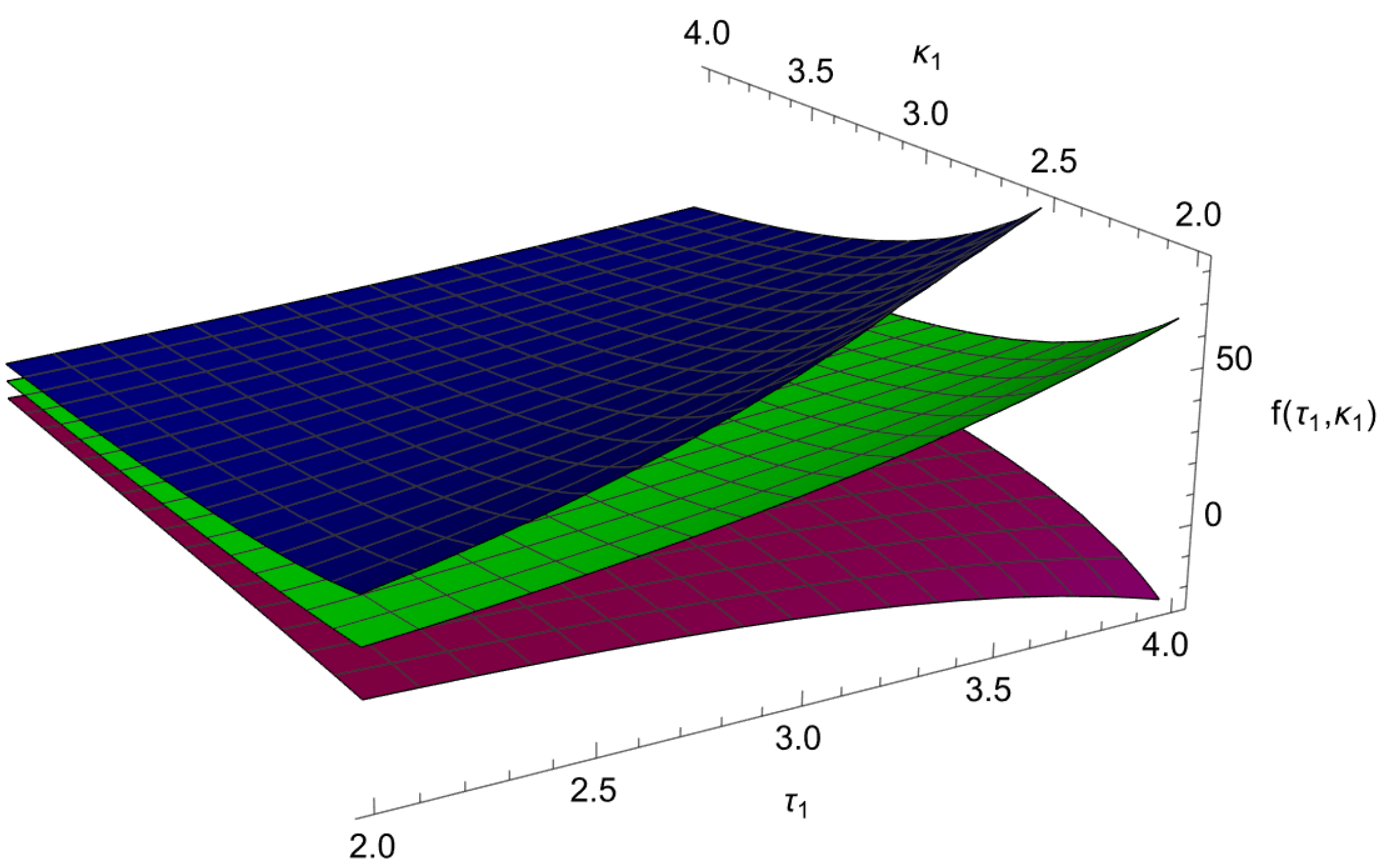
Figure 2 justifies that the bounds of the mean value integral are correct by keeping ${\tau }_1,{\kappa }_1\in [2,4]$ as unknowns. Here, we provide the tabular explanation of the above expressions.

Figure 2. Graphical validation of Theorem 4.

Table 2 illustrates how the variation in ${\kappa }_1$ influences the bounds, which confirms the accuracy of Theorem 4.

Table 2. Bounds for the mean integral.

$({\mathit{\tau }}_1,{\mathit{\kappa }}_1)$	${\mathit{T}}_1$	${\mathit{T}}_2$	${\mathit{T}}_3$
$(2,2)$	$3.16$	18	$32.83$
$(2,3)$	4	$12.1571$	$20.34$
$(2,4)$	$4.03$	$10.0779$	$16.15$
$(2,5)$	$3.98$	$9.03385$	$14.11$
$(2,6)$	$3.92$	$8.41067$	$12.91$
$(2,7)$	$3.88$	$7.99797$	$12.13$
$(2,8)$	$3.84$	$7.70503$	$11.58$

Theorem 5. 

Assume that $f:[a,b]\to$ is an nth-order differentiable mapping. If $|f^n|$ is a bounded mapping such that $|f^n|\le {\kappa }_1$, then

$$\begin{array}{cc}\hfill & \left|{\displaystyle \sum _{k=0}^{n-1}}{\displaystyle \frac{{\left(\mathcal{l}\right)}^k}{(k+1)2^{k+1}}}\left\{\left[{\left({\displaystyle \frac{5}{12}}\right)}^{k+1}+{(-1)}^k{\left({\displaystyle \frac{1}{3}}\right)}^{k+1}\right]f^k\left(x_1\right)+\left[{\left({\displaystyle \frac{1}{4}}\right)}^{k+1}+{(-1)}^k{\left({\displaystyle \frac{1}{4}}\right)}^{k+1}\right]\times \right.\right.\hfill \\ & \left.\left.f^k\left(x_2\right)+\left[{\left({\displaystyle \frac{1}{3}}\right)}^{k+1}+{(-1)}^k{\left({\displaystyle \frac{5}{12}}\right)}^{k+1}\right]f^k\left(x_3\right)\right\}-{\displaystyle \frac{1}{\mathcal{l}}}{\int }_a^{b}f\left(u\right)\mathrm{d}u\right|\hfill \\ \hfill & \le {\displaystyle \frac{2{\kappa }_1{\left(\mathcal{l}\right)}^n\left(3^{n+1}+4^{n+1}+5^{n+1}\right)}{{24}^{n+1}(n+1)!}}.\hfill \end{array}$$

Proof. 

Considering Equation (3) and implementing the modulus and bounded property of $|f^n|$ yields

$$\begin{array}{cc}\hfill & \left|{\displaystyle \sum _{k=0}^{n-1}}{\displaystyle \frac{{\left(\mathcal{l}\right)}^k}{(k+1)2^{k+1}}}\left\{\left[{\left({\displaystyle \frac{5}{12}}\right)}^{k+1}+{(-1)}^k{\left({\displaystyle \frac{1}{3}}\right)}^{k+1}\right]f^k\left(x_1\right)+\left[{\left({\displaystyle \frac{1}{4}}\right)}^{k+1}+{(-1)}^k{\left({\displaystyle \frac{1}{4}}\right)}^{k+1}\right]\times \right.\right.\hfill \\ & \left.\left.f^k\left(x_2\right)+\left[{\left({\displaystyle \frac{1}{3}}\right)}^{k+1}+{(-1)}^k{\left({\displaystyle \frac{5}{12}}\right)}^{k+1}\right]f^k\left(x_3\right)\right\}-{\displaystyle \frac{1}{\mathcal{l}}}{\int }_a^{b}f\left(u\right)\mathrm{d}u\right|\hfill \\ \hfill & \le {\displaystyle \frac{{\left(\mathcal{l}\right)}^n}{2^{n+1}n!}}\left[{\int }_0^{{\displaystyle \frac{2}{3}}}{\left|\gamma -{\displaystyle \frac{1}{4}}\right|}^n\left|f^n\left({\displaystyle \frac{a+\gamma \mathcal{l}+b}{2}}\right)\right|\mathrm{d}\gamma +{\int }_0^{{\displaystyle \frac{2}{3}}}{\left|\gamma -{\displaystyle \frac{1}{4}}\right|}^n\left|f^n\left({\displaystyle \frac{a-\gamma \mathcal{l}+b}{2}}\right)\right|\mathrm{d}\gamma \right.\hfill \\ \hfill & \left.+{\int }_{{\displaystyle \frac{2}{3}}}^1{\left|1-\gamma \right|}^n\left|f^n\left({\displaystyle \frac{a+\gamma \mathcal{l}+b}{2}}\right)\right|\mathrm{d}\gamma +{\int }_{{\displaystyle \frac{2}{3}}}^1{\left|1-\gamma \right|}^n\left|f^n\left({\displaystyle \frac{a-\gamma \mathcal{l}+b}{2}}\right)\right|\mathrm{d}\gamma \right]\hfill \\ \hfill & \le {\displaystyle \frac{2{\kappa }_1{\left(\mathcal{l}\right)}^n}{2^{n+1}n!}}\left[{\int }_0^{{\displaystyle \frac{2}{3}}}{\left|\gamma -{\displaystyle \frac{1}{4}}\right|}^n\mathrm{d}\gamma +{\int }_{{\displaystyle \frac{2}{3}}}^1{\left|1-\gamma \right|}^n\mathrm{d}\gamma \right].\hfill \end{array}$$

   □

Corollary 4. 

Setting $n=1$ in Theorem 5, we obtain

$$\begin{array}{cc}\hfill & \left|{\displaystyle \frac{1}{8}}\left[3f\left(x_1\right)+2f\left(x_2\right)+3f\left(x_3\right)\right]-{\displaystyle \frac{1}{\mathcal{l}}}{\int }_a^{b}f\left(x\right)\mathrm{d}x\right|\le {\displaystyle \frac{50{\kappa }_1\left(\mathcal{l}\right)}{576}}\left[|f^{\prime }\left(a\right)|+|f^{\prime }\left(b\right)|\right].\hfill \end{array}$$

Here, we give the explanation of Theorem 1 in terms of the mean value integral by taking the means of $f\left(x\right)={\displaystyle \frac{{\kappa }_1}{{\tau }_1+2{\kappa }_1}}{x}^{{\displaystyle \frac{{\tau }_1}{{\kappa }_1}}+2},{\tau }_1\ge 1$, ${\kappa }_1>1$ and $[a,b]=[0,6]$.

$$\begin{array}{c}\hfill T_1={\displaystyle \frac{{\kappa }_1\left[3\left(5^{\frac{2{\kappa }_1+{\tau }_1}{{\kappa }_1}}\right)+2\left(3^{\frac{2{\kappa }_1+{\tau }_1}{{\kappa }_1}}\right)+3\right]}{8(2{\kappa }_1+{\tau }_1)}}-{\displaystyle \frac{25\left(6^{\frac{{\tau }_1+2{\kappa }_1}{{\kappa }_1}}\right)}{288}}.\end{array}$$

$$\begin{array}{c}\hfill T_2={\displaystyle \frac{{{\kappa }_1}^2\left(6^{\frac{2{\kappa }_1+{\tau }_1}{{\kappa }_1}}\right)}{({\tau }_1+2{\kappa }_1)({\tau }_1+3{\kappa }_1)}}.\end{array}$$

$$\begin{array}{c}\hfill T_3={\displaystyle \frac{{\kappa }_1\left[3\left(5^{\frac{2{\kappa }_1+{\tau }_1}{{\kappa }_1}}\right)+2\left(3^{\frac{2{\kappa }_1+{\tau }_1}{{\kappa }_1}}\right)+3\right]}{8(2{\kappa }_1+{\tau }_1)}}+{\displaystyle \frac{25\left(6^{\frac{{\tau }_1+2{\kappa }_1}{{\kappa }_1}}\right)}{288}}.\end{array}$$

Figure 3 provides the bounds for the mean value integral by keeping ${\tau }_1,{\kappa }_1\in [2,4]$ as unknowns. Here, we provide the tabular explanation of the above expressions.

Figure 3. Graphical analysis of Theorem 5.

Table 3 provide the numerical breakdown of Theorem 5 under certain functions.

Table 3. Numerical comparison of Theorem 5.

$({\mathit{\tau }}_1,{\mathit{\kappa }}_1)$	${\mathit{T}}_1$	${\mathit{T}}_2$	${\mathit{T}}_3$
$(2,2)$	$-0.75$	18	$36.75$
$(2,3)$	$1.85$	$12.1571$	$22.49$
$(2,4)$	$2.43$	$10.0779$	$17.74$
$(2,5)$	$2.64$	$9.03385$	$15.44$
$(2,6)$	$2.74$	$8.41067$	$14.10$
$(2,7)$	$2.79$	$7.99797$	$13.22$
$(2,8)$	$2.82$	$7.70503$	$12.60$

2.2. Comparison Analysis

In this section we give a brief comparison of our obtained result (3) with some classical results. Moreover, we provide the numerical comparison of Maclaurin’s inequality [25], Simpson’s inequality [4] and Theorem 3 for $f\left(\varrho \right)={\varrho }^3$ for $q=1$ with $a=0$ and $b=2$, which is as follows:

• Classical Maclaurin Inequality: 0 < 1.0416;
• Simpson Inequality: 0 < 1.6666;
• Inequality (9): 0 < 0.3941.

3. Analysis of Maclaurin Inequality Through Artificial Neural Networks

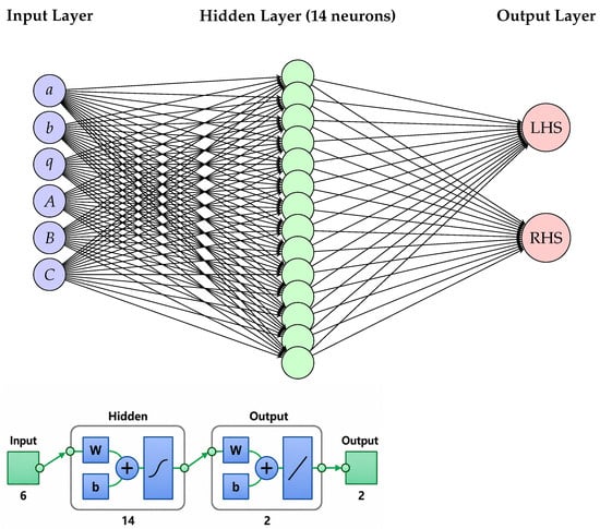
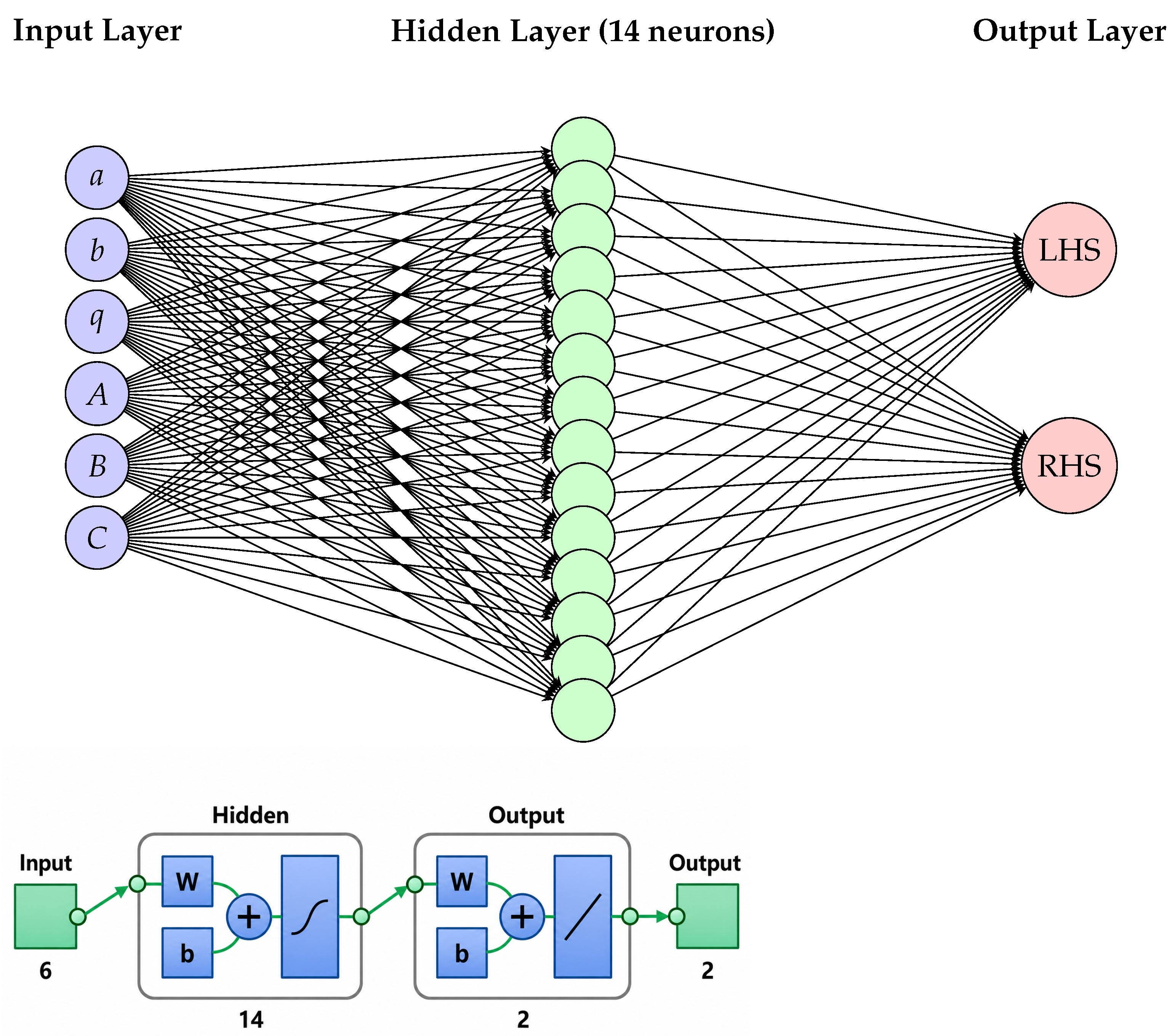
This part of the study is concerned with the implementation of an ANN technique to validate and predict the estimates of the higher-order Maclaurin inequality. We used a general class of functions with different input parameters, and the output was formulated to assess the inequality given in Theorem 3. A feed-forward ANN network with an input layer with six parameters, hidden layer based on 14 neurones and output layer with two points was considered. The ANN modeling was conducted using the MATLAB (R2022a) Neural Network Toolbox. We constructed a sample of $N=3000$ data points via quadratic function $A{x}^2+Bx+C$ with the following input variables:

• $A\in [1,4]$;
• $B\in [-2,2]$;
• $C\in [-1,1]$;
• $a\in [-2,2]$;
• $b\in [a+0.5,a+2.5]$;
• $q=[1,3]$.

Moreover, the logarithmic sigmoid function was selected as an activation function to tackle the nonlinearity in the network. We tested the model with four to 20 neurons in the hidden layer. For less than 14 neurons, the ANN model underestimated the data and with more than 14 neurons, it overestimated the data; optimal values were obtained with 14 neurons. For reproducibility, we used the twister algorithm with 10 seeds, and the failure of six consecutive validations was fixed as an early-stopping criteria. This model also provided the behavior of inequalities when varying the parameters. For the enhancement of the process, the mapminmax function was used for the normalization purpose of both input and output data. The data were classified in three categories, seventy percent for training and 15 percent for validation and testing, respectively.

Figure 4 illustrates the procedure of the network. Its details are already described in the introductory part. It is interesting to note that A, B, C, a, b and q are non-zero parameters, while the output values predict the values for left and right sides. The training was directly linked with the mean square error by using Levenberg–Marquardt (trainlm) as the training algorithm, tansig as a transfer function for the hidden layer, and purelin as the transfer function for the output layer. The mean square error is defined as:

$$\begin{array}{c}\hfill \mathrm{Mean}\mathrm{Square}\mathrm{Error}={\displaystyle \frac{1}{n}}{\displaystyle \sum _{i=1}^n}{(y_i-{\widehat{y}}_i)}^2,\end{array}$$

where ${\widehat{y}}_i$ are predicted and $y_i$ are the actual values with n total points. The accuracy of the model has an inverse relation with the mean square error. That is why it has a key role in the learning process.

Figure 4. Flow chart of neural network model operating with 6 input variables $(a,b,q,A,B,C)$, 14 neurons in the hidden layer and 2 output variables with left- and right-hand sides, respectively.

The efficacy of the network was also checked using the correlation coefficient R, which associates the correlation between actual and predicted bounds of the inequality. It is stated as

$$\begin{array}{c}\hfill R={\displaystyle \frac{{\sum }_{i=1}^n(y_i-\overline{y})({\widehat{y}}_i-\overline{\widehat{y}})}{\sqrt{{\sum }_{i=1}^n{(y_i-\overline{y})}^2{\sum }_{i=1}^n{({\widehat{y}}_i-\overline{\widehat{y}})}^2}}},\end{array}$$

where $\overline{\widehat{y}}$ and $\overline{y}$ are the mean values of actual and predicted values, respectively. Its values are bounded between −1 and one. In the case of R = 1, the estimated values are suitable and −1 refers to non-related values.

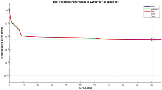
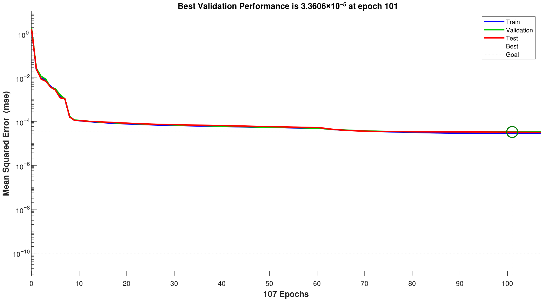
Figure 5 reflects the gradual decrement in mean square error with respect to time; the best validation marks are attained at epochs 101. Observe that the error is slightly high in the early epochs. Additionally, the figure contains the error analysis of all three stages. The gradual decrement error reaches an optimal value for better performance of the network. For more details regarding training performance, see the following metric:

Figure 5. Mean square error distribution across training, testing and validation.

1.

Epochs completed: 107/150;

2.

Final Training MSE: 2.843237 × 10⁻⁰⁵;

3.

Final Validation MSE: 3.366237 × 10⁻⁰⁵;

4.

Final Testing MSE: 3.254879 × 10⁻⁰⁵;

5.

Best Validation Epoch: 101;

6.

Training stopped: Validation stop.

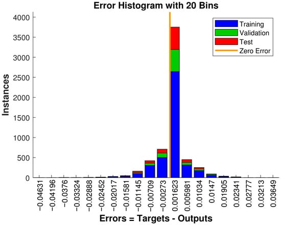
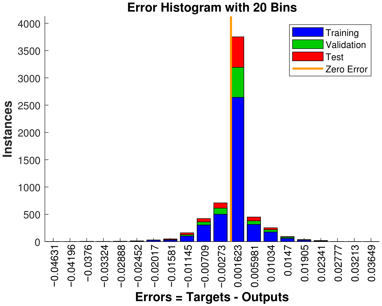
In Figure 6, we present the error between exact and estimated values. It illustrates the frequency of errors with respect to training, testing, and validation. One can see that errors are gathered around zero, which reflects that the model is well trained and estimating accurately.

Figure 6. Error histogram of neural network model to approximate both sides of Theorem 3.

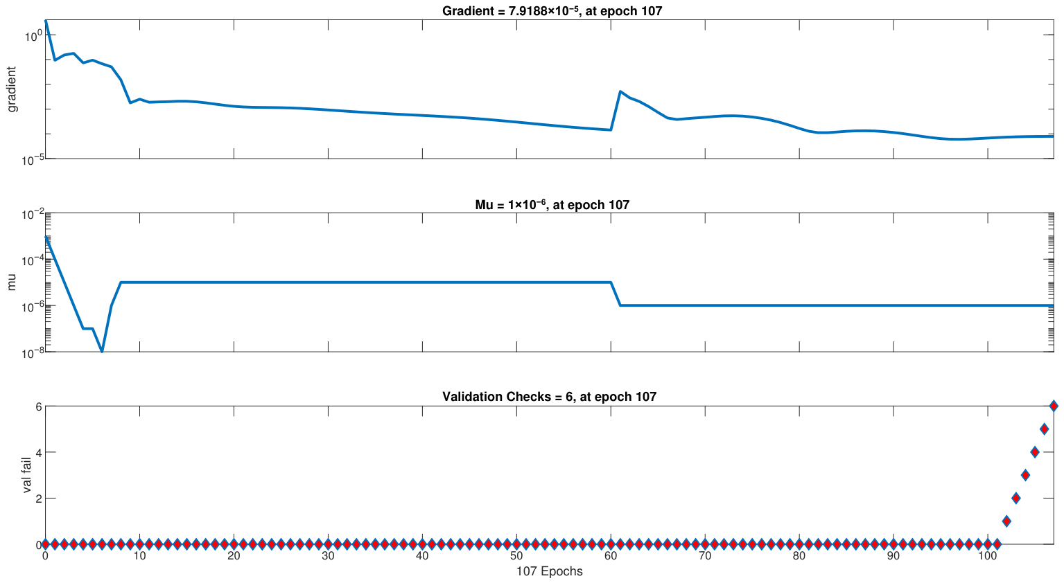
The behavior of the gradient of the loss function showcases the learning rate. To adjust parameters like weights and biases, the direction of the gradient is illustrated at each epoch in Figure 7. Initially the values of the gradient are slightly greater and highlight the fast learning rate; gradually, it approaches a moderate rate with optimal values of weights and biases.

Figure 7. Gradient behavior of model to adjust the weight and biases and attain the optimal values.

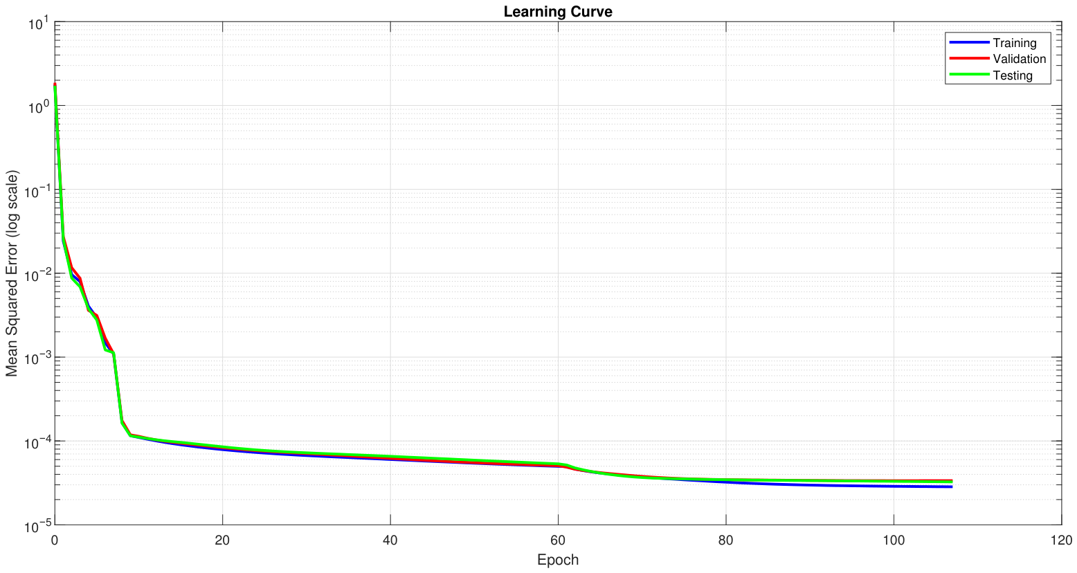
Figure 8 (learning curve) shows that convergence is achieved in the first 20 epochs where training, validation and test errors are reduced in a parallel manner, from ${10}^{-1}$ to ${10}^{-4}$. The lack of curve divergence indicates that the 14-neuron architecture is able to generalize well without over-fitting.

Figure 8. Gradient behavior of model to adjust the weight and biases to attain the optimal values.

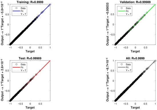
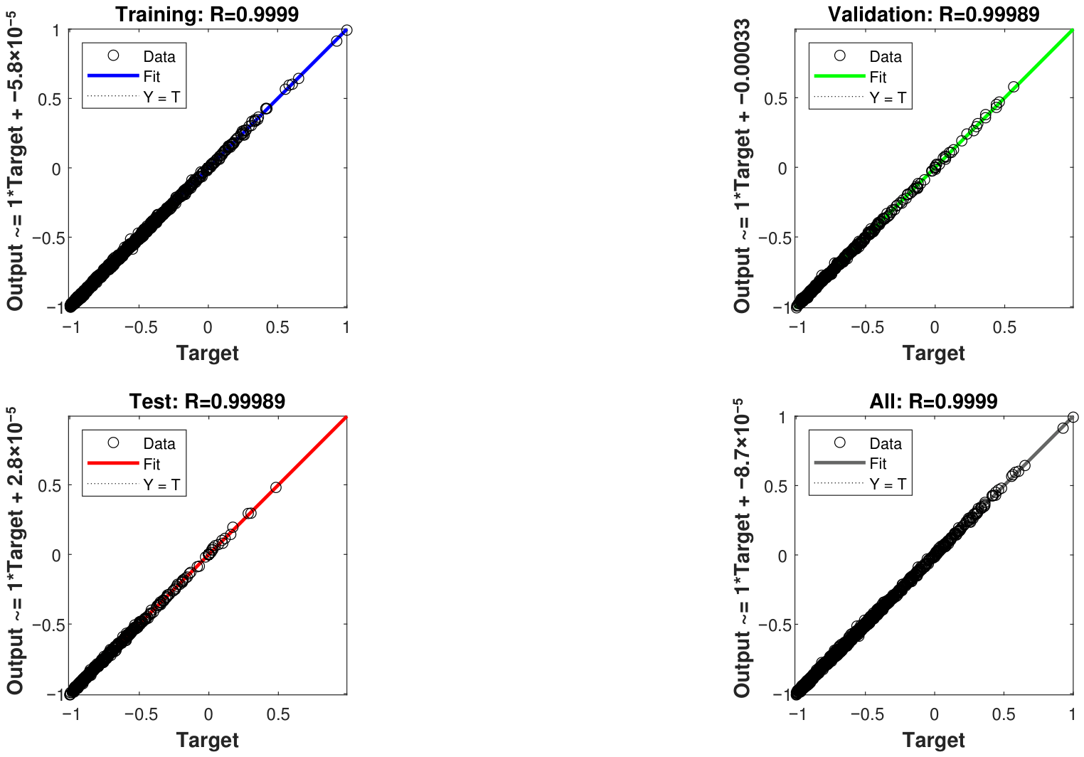
Figure 9 contains regression plots illustrating the correlation between predicted and exact values. The high value for all phases confirms that the model is well trained. Its high value does not indicate over-fitting because we selected a general class of quadratic functions, and Maclaurin rule is exact for polynomials of degree less than three.

Figure 9. Confirmation of model through correlation technique.

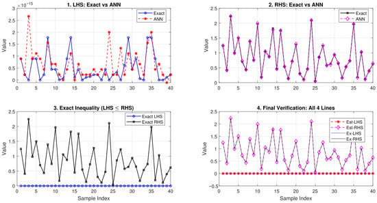
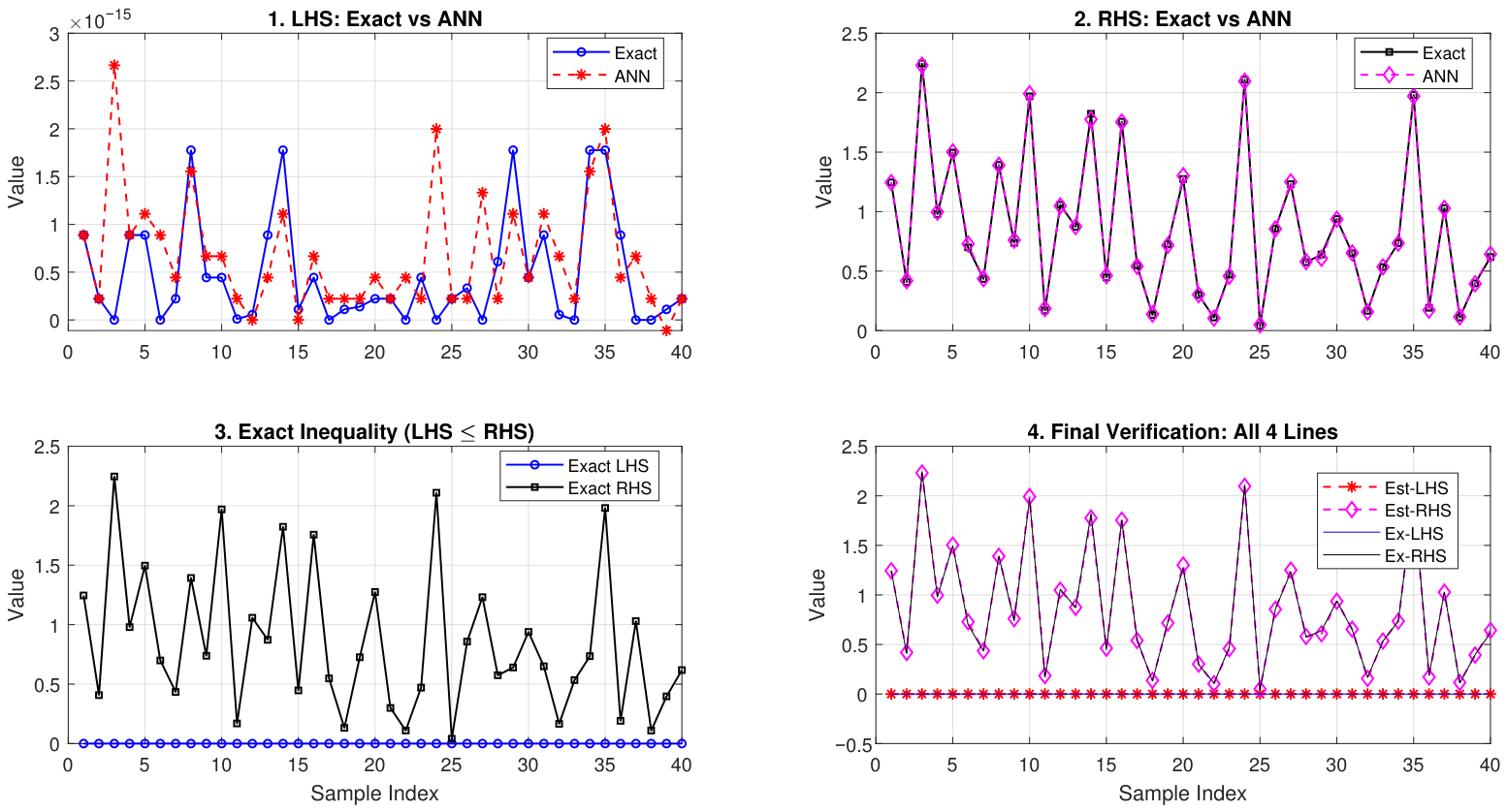
Figure 10 demonstrates the accuracy of Theorem 3 through the above trained neural network model. The sub-figures contain the comparative information regarding predicted and exact values of each side and finally a combined graph of exact and approximated values representing the comparison between both sides of Theorem 3.

Figure 10. Comparison between sides of Theorem 3 through our ANN technique.

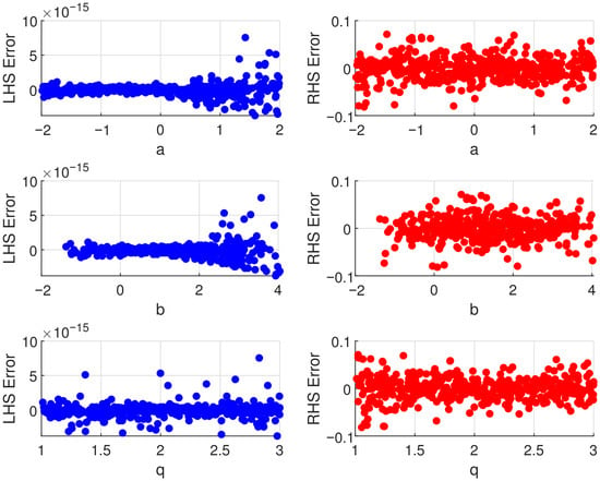
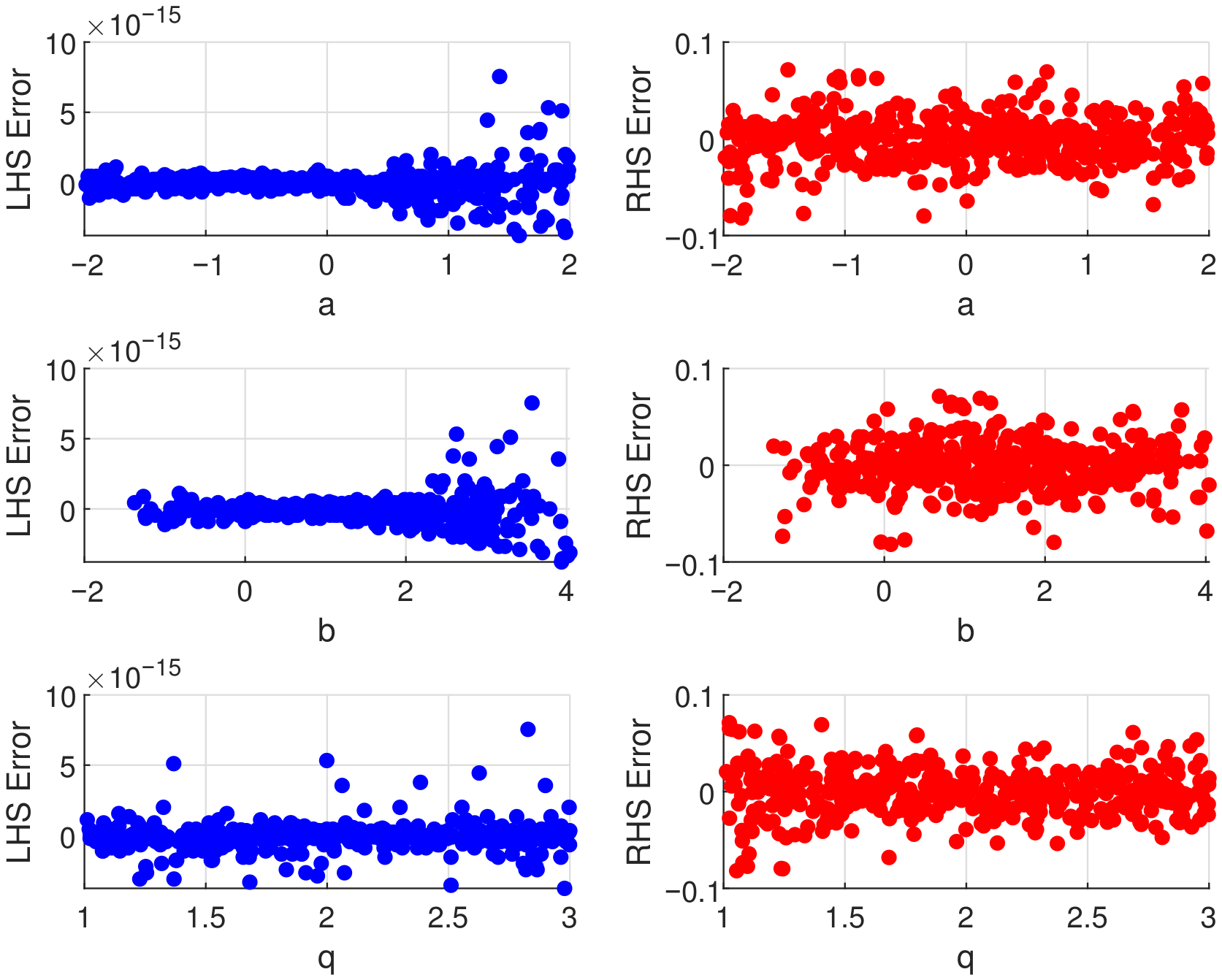
The error analysis of both sides depending upon different parameters are given in Figure 11. One can observe the influence of a, b and q on the error of both sides of the inequality.

Figure 11. Scatter plot of both left- and right-side errors, respectively.

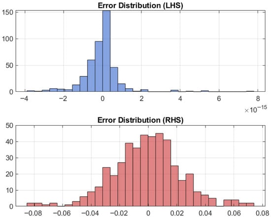
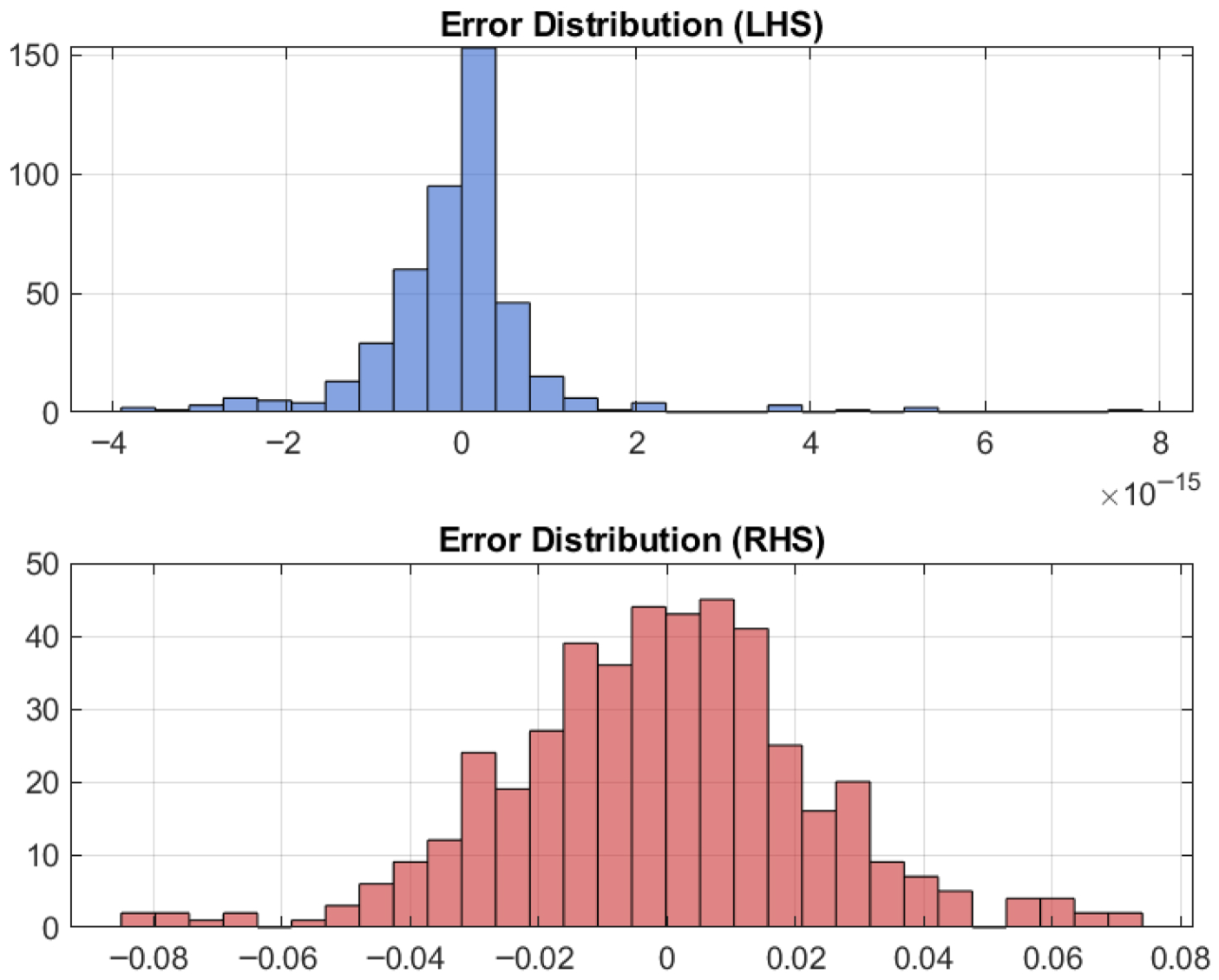
Figure 12 provides histograms of the error distributions and frequency for both sides of the inequality established in Theorem 3. The blue and red colors represent the analysis for the left and right sides, respectively.

Figure 12. Error and frequency distribution of errors for both left and right sides, respectively.

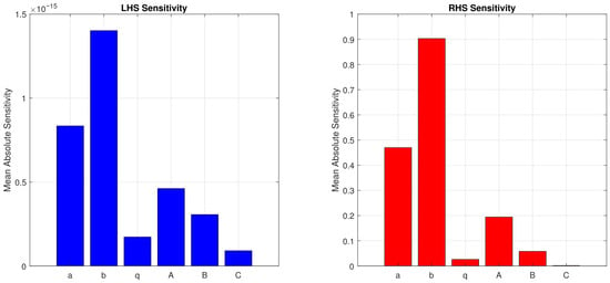
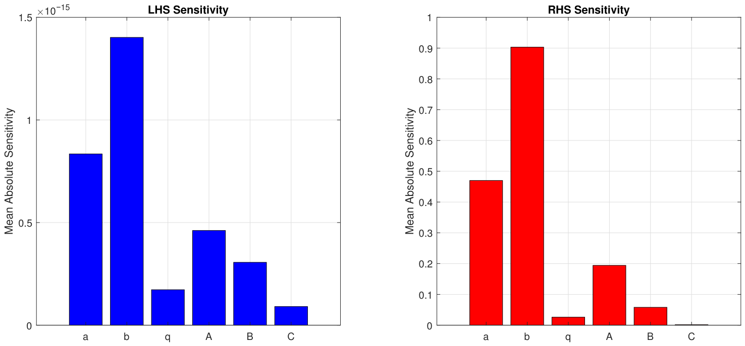
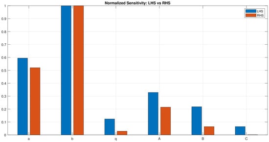
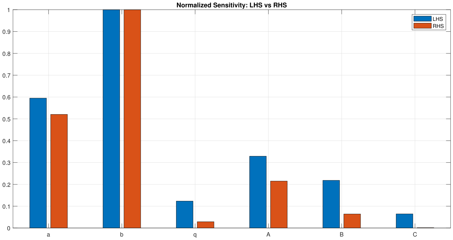
Figure 13 and Figure 14 showcase the impact of the variation in input variables on output values. It has already been shown that left- and right-end points of intervals and quadratic-term coefficients affect the sides of inequalities. For a comprehensive investigation, see the following Table 4.

Figure 13. Sensitivity of all parameters with respect to both sides of Theorem 3.

Figure 14. Normalized sensitivity analysis of Theorem 3.

Table 4. Sensitivity analysis (mean absolute sensitivity).

Parameter	LHS	RHS
a	8.34 × 10−16	$1.403949$
b	1.40 × 10−15	$2.697616$
q	1.73 × 10−16	$0.077464$
A	4.61 × 10−16	$0.580030$
B	3.06 × 10−16	$0.173232$
C	9.07 × 10−17	$0.004216$

Last, we present the pseudo-code in Algorithm 1 to reproduce the graphical analysis.

Algorithm 1 ANN modeling for Maclaurin’s inequality under $q\ge 1$ conditions

1: Input: Sample size $N=3000$, bounds $[a,b]$, parameter $q\ge 1$, coefficients $A,B,C$.  2: Output: Trained ANN model, performance metrics ($MSE,R$), sensitivity analysis S. Phase 1: Dataset Preparation  3: for  $i=1$  to  N  do  4:        Generate random $a,b\in \mathbb{R}$ ($b>a$) and parameter $q\in [1,3]$  5:        Define $f\left(x\right)=A{x}^2+Bx+C$ and its derivative $|f^{\prime }{\left(x\right)|}^q={|2Ax+B|}^q$  6:        LHS calculation (Maclaurin form):  7:        Compute nodes $x_1={\displaystyle \frac{5a+b}{6}},x_2={\displaystyle \frac{a+b}{2}},x_3={\displaystyle \frac{a+5b}{6}}$  8:        $LH{S}_i\leftarrow \left|{\displaystyle \frac{1}{8}}[3f\left(x_1\right)+2f\left(x_2\right)+3f\left(x_3\right)]-{\displaystyle \frac{1}{b-a}}{\int }_a^{b}f\left(u\right)du\right|$  9:        RHS calculation (theorem bound): 10:        Calculate $S_1$ using $|f^{\prime }{\left(a\right)|}^q,{\left|f^{\prime }\left(b\right)\right|}^q$ and constants $\{{\displaystyle \frac{17}{144}},{\displaystyle \frac{361}{10368}},{\displaystyle \frac{863}{10368}}\}$ 11:        Calculate $S_2$ using $|f^{\prime }{\left(a\right)|}^q,{\left|f^{\prime }\left(b\right)\right|}^q$ and constants $\{{\displaystyle \frac{1}{18}},{\displaystyle \frac{1}{162}},{\displaystyle \frac{8}{162}}\}$ 12:        $RH{S}_i\leftarrow {\displaystyle \frac{b-a}{4}}(S_1+S_2)$ 13: end for 14: Filter dataset $\mathcal{D}$ to retain samples where $LH{S}_i\le RH{S}_i$ Phase 2: Artificial Neural Network Training 15: Normalize input matrix $X_{6\times N}$ and target matrix $Y_{2\times N}$ to $[-1,1]$ 16: Initialize feed-forward ANN with 14 hidden neurons (Levenberg–Marquardt) 17: Partition data: $70\%$ training, $15\%$ validation, $15\%$ testing 18: Train network until $MSE\le {10}^{-10}$ or 150 epochs are reached Phase 3: Diagnostic Analysis and Sensitivity 19: Evaluate $MSE,RMSE,$ and Correlation R for the testing partition 20: for each input parameter $j\in \{a,b,q,A,B,C\}$ do 21:        Compute mean absolute sensitivity $S_j={\displaystyle \frac{1}{N}}{\sum }_{k=1}^N\left|{\displaystyle \frac{net(X_j+\delta )-net(X_j-\delta )}{2\delta }}\right|$ 22: end for 23: Generate learning curve (including test MSE), regression, and sensitivity plots

In the next part, we leverage several important implications of our primary findings.

3.1. Bounds of Differences Between Means

Consider some well-known means of non-negative real numbers:

1.

The arithmetic mean:

$$A(a,b)={\displaystyle \frac{a+b}{2}},$$

2.

The weighted arithmetic mean:

$${}_{w}A(w_1,w_2;a,b)={\displaystyle \frac{a{w}_1+b{w}_2}{w_1+w_2}}.$$

3.

The log-mean:

$$L_{{\tau }_1}(a,b)={\left[{\displaystyle \frac{b^{{\tau }_1+1}-a^{{\tau }_1+1}}{({\tau }_1+1)(b-a)}}\right]}^{{\displaystyle \frac{1}{{\tau }_1}}};{\tau }_1\in \Re \setminus \{-1,0\}.$$

Proposition 1. 

For $a,b\ge 0$, we have

$$\begin{array}{cc}\hfill & \left|{\displaystyle \sum _{k=0}^{n-1}}{\displaystyle \frac{{\kappa }_1!{\left(\mathcal{l}\right)}^k}{(k+1)2^{k+1}({\kappa }_1-k)!}}\left\{\left[{\left({\displaystyle \frac{5}{12}}\right)}^{k+1}+{(-1)}^k{\left({\displaystyle \frac{1}{3}}\right)}^{k+1}\right]A_w^{{\kappa }_1-k}(a,b;5,1)+\right.\right.\hfill \\ \hfill & \left.\left.\left[{\left({\displaystyle \frac{1}{4}}\right)}^{k+1}+{(-1)}^k{\left({\displaystyle \frac{1}{4}}\right)}^{k+1}\right]A^{{\kappa }_1-k}(a,b)+\left[{\left({\displaystyle \frac{1}{3}}\right)}^{k+1}+{(-1)}^k{\left({\displaystyle \frac{5}{12}}\right)}^{k+1}\right]A_w^{{\kappa }_1-k}(a,b;1,5)\right\}-{Ł}_{{\kappa }_1}^{{\kappa }_1}(a,b)\right|\hfill \\ \hfill & \le {\displaystyle \frac{2{\kappa }_1!{\left(\mathcal{l}\right)}^n\left(3^{n+1}+4^{n+1}+5^{n+1}\right)}{{(-1)}^{n+1}{24}^{n+1}(n+1)!({\kappa }_1-n)!}}A\left(|a^{{\kappa }_1-n}|,|b^{{\kappa }_1-n}|\right).\hfill \end{array}$$

Proof. 

The assertion follows directly by substitution of $f\left(x\right)=x^{{\kappa }_1},{\kappa }_1>n$, in Theorem 1. □

Now, we discuss some consequences of Proposition 1.

• Choosing $n=1$ in Proposition 1, we get the following relation between the means:

  $$\begin{array}{cc}\hfill & \left|{\displaystyle \frac{1}{8}}\left\{3A_w^{{\kappa }_1}(a,b;5,1)+2A^{{\kappa }_1}(a,b)+3A_w^{{\kappa }_1}(a,b;1,5)\right\}-{Ł}_{{\kappa }_1}^{{\kappa }_1}(a,b)\right|\hfill \\ \hfill & \le {\displaystyle \frac{25{\kappa }_1\left(\mathcal{l}\right)}{288}}A\left(|a^{{\kappa }_1-1}|,|b^{{\kappa }_1-1}|\right).\hfill \end{array}$$
• Choosing $n=2$ in Proposition 1, we get the following relation between the means:

  $$\begin{array}{cc}\hfill & \left|{\displaystyle \frac{1}{8}}\left\{3A_w^{{\kappa }_1}(a,b;5,1)+2A^{{\kappa }_1}(a,b)+3A_w^{{\kappa }_1}(a,b;1,5)\right\}\right.\hfill \\ \hfill & \left.+{\displaystyle \frac{{\kappa }_1\left(\mathcal{l}\right)}{128}}\left[A_w^{{\kappa }_1-1}(a,b;5,1)-A_w^{{\kappa }_1-1}(a,b;1,5)\right]-{Ł}_{{\kappa }_1}^{{\kappa }_1}(a,b)\right|\hfill \\ \hfill & \le {\displaystyle \frac{{\kappa }_1({\kappa }_1-1){\left(\mathcal{l}\right)}^2}{192}}A\left(|a^{{\kappa }_1-2}|,|b^{{\kappa }_1-2}|\right).\hfill \end{array}$$

3.2. Composite Refined Error Estimates

Here, we develop some fresh error inequalities of the composite rule for first-order differentiable mappings via convex mappings. Let us consider the division of $[a,b]$ such that $\P =:\{a=x_0,x_1,x_2,...,x_n=b\}$. Recall that Euler-Maclaurin’s scheme is described as:

$$\begin{array}{c}\hfill {\int }_a^{b}f\left(x\right)dx={\mathcal{C}}_{\circ }\left(x\right)+R\left(x\right).\end{array}$$

Here,

$$\begin{array}{c}\hfill {\mathcal{C}}_{\circ }\left(x\right)={\displaystyle \sum _{i=0}^{n-1}}{\displaystyle \frac{x_{i+1}-x_i}{8}}\left(3f\left({\displaystyle \frac{5x_i+x_{i+1}}{6}}\right)+2f\left({\displaystyle \frac{x_i+x_{i+1}}{2}}\right)+3f\left({\displaystyle \frac{x_i+5x_{i+1}}{6}}\right)\right)\end{array}$$

and $R\left(x\right)$ is declared as an error term.

Proposition 2. 

From the assumptions of Theorem 4, we have

$$\begin{array}{cc}\hfill & \left|R\right(x\left)\right|\hfill \\ \hfill & \le {\displaystyle \sum _{i=0}^{n-1}}{\displaystyle \frac{{(x_{i+1}-x_i)}^2}{4}}\left[{\left({\displaystyle \frac{{\left(\frac{5}{12}\right)}^{p+1}+4^{-p-1}}{p+1}}\right)}^{{\displaystyle \frac{1}{p}}}\left({\left({\displaystyle \frac{2|f^{\prime }\left(x_i\right){|}^{\mathfrak{q}}+4{\left|f^{\prime }\left(x_{i+1}\right)\right|}^{\mathfrak{q}}}{9}}\right)}^{{\displaystyle \frac{1}{\mathfrak{q}}}}+{\left({\displaystyle \frac{4|f^{\prime }\left(x_i\right){|}^{\mathfrak{q}}+2{\left|f^{\prime }\left(x_{i+1}\right)\right|}^{\mathfrak{q}}}{9}}\right)}^{{\displaystyle \frac{1}{\mathfrak{q}}}}\right)\right.\hfill \\ \hfill & \left.+{\left({\displaystyle \frac{3^{-p-1}}{p+1}}\right)}^{{\displaystyle \frac{1}{p}}}\left({\left({\displaystyle \frac{|f^{\prime }\left(x_i\right){|}^{\mathfrak{q}}+11{\left|f^{\prime }\left(x_{i+1}\right)\right|}^{\mathfrak{q}}}{36}}\right)}^{{\displaystyle \frac{1}{\mathfrak{q}}}}+{\left({\displaystyle \frac{11|f^{\prime }\left(x_i\right){|}^{\mathfrak{q}}+{\left|f^{\prime }\left(x_{i+1}\right)\right|}^{\mathfrak{q}}}{36}}\right)}^{{\displaystyle \frac{1}{\mathfrak{q}}}}\right)\right].\hfill \end{array}$$

Proof. 

By choosing $n=1$ in Theorem 4, applying it over $[x_i,x_{i+1}]$, and finally taking the sum from $i=0$ to $n-1$, we acquire our intended outcome. □

Proposition 3. 

From the assumptions of Theorem 5, we have

$$\begin{array}{cc}\hfill & \left|R\left(x\right)\right|\le {\displaystyle \sum _{i=0}^{n-1}}{\displaystyle \frac{25M{(x_{i+1}-x_i)}^2}{288}}.\hfill \end{array}$$

Proof. 

By choosing $n=1$ in Theorem 5, applying it over $[x_i,x_{i+1}]$, and finally taking the sum from $i=0$ to $n-1$, we acquire our intended outcome. □

3.3. Development of Boundaries for Probability Density Mappings

Let $\mathfrak{P}:[a,b]\to [0,1]$ be a probability density and its associated cumulative mappings given by

$$\begin{array}{cc}\hfill & Pr(x\le b)=f\left(b\right)={\int }_a^b\mathfrak{P}\left(\gamma \right)\mathrm{d}\gamma .\hfill \end{array}$$

Utilizing the fact that

$$\begin{array}{cc}\hfill & E\left(x\right)={\int }_a^b\gamma \mathfrak{P}\left(\gamma \right)\mathrm{d}\gamma \hfill \\ \hfill & E\left(x\right)=b-{\int }_a^b\mathfrak{P}\left(\gamma \right)\mathrm{d}\gamma .\hfill \end{array}$$

Proposition 4. 

From the assumptions of Theorem 1, we have the following relation:

$$\begin{array}{cc}\hfill & \left|{\displaystyle \frac{1}{8}}\left[3Pr\left(x\le x_1\right)+2Pr\left(x\le x_2\right)+3Pr\left(x\le x_3\right)\right]-{\displaystyle \frac{b-E\left(x\right)}{\mathcal{l}}}\right|\hfill \\ \hfill & \le {\displaystyle \frac{25\left(\mathcal{l}\right)}{576}}\left[\left|\mathfrak{P}\right(a\left)\right|+\left|\mathfrak{P}\right(b\left)\right|\right].\hfill \end{array}$$

Proof. 

The proof is simply acquired from Theorem 1 by taking $n=1=\mathfrak{q}$. □

3.4. Inequalities for $\mathfrak{q}$-Digamma Mappings

The class of $\mathfrak{q}$-digamma ${\Psi }_{{\mathfrak{q}}_1}\left(\mathfrak{u}\right)$ mappings and its representation are given by

$$\begin{array}{cc}\hfill {\Psi }_{{\mathfrak{q}}_1}\left(\mathfrak{u}\right)& =-ln(1-{\mathfrak{q}}_1)+ln\left({\mathfrak{q}}_1\right){\displaystyle \sum _{i=0}^{\infty }}{\displaystyle \frac{{{\mathfrak{q}}_1}^{i+\mathfrak{u}}}{1-{{\mathfrak{q}}_1}^{i+\mathfrak{u}}}}.\hfill \\ \hfill & =-ln(1-{\mathfrak{q}}_1)+ln\left({\mathfrak{q}}_1\right){\displaystyle \sum _{i=0}^{\infty }}{\displaystyle \frac{{{\mathfrak{q}}_1}^{iu}}{1-{{\mathfrak{q}}_1}^{iu}}}.\hfill \end{array}$$

For $\mathfrak{u}>0$ and ${\mathfrak{q}}_1>1$, ${\Psi }_{{\mathfrak{q}}_1}$ can be interpreted as

$$\begin{array}{cc}\hfill {\Psi }_{{\mathfrak{q}}_1}\left(\mathfrak{u}\right)& =-ln({\mathfrak{q}}_1-1)+ln\left({\mathfrak{q}}_1\right)\left[\mathfrak{u}-{\displaystyle \frac{1}{2}}-{\displaystyle \sum _{i=0}^{\infty }}{\displaystyle \frac{{{\mathfrak{q}}_1}^{-(i+\mathfrak{u})}}{1-{{\mathfrak{q}}_1}^{-(i+\mathfrak{u})}}}\right]\hfill \\ \hfill & =-ln({\mathfrak{q}}_1-1)+ln\left({\mathfrak{q}}_1\right)\left[\mathfrak{u}-{\displaystyle \frac{1}{2}}-{\displaystyle \sum _{i=0}^{\infty }}{\displaystyle \frac{{{\mathfrak{q}}_1}^{-iu}}{1-{{\mathfrak{q}}_1}^{-iu}}}\right].\hfill \end{array}$$

It is not hard to prove that ${\Psi }_{{\mathfrak{q}}_1}^{\prime }\left(\mathfrak{u}\right)$ possesses the convexity property.

Proposition 5. 

From Theorem 1, we achieve

$$\begin{array}{cc}\hfill & \left|{\displaystyle \frac{1}{8}}\left[3{\Psi }^{\prime }\left(x_1\right)+2{\Psi }^{\prime }\left(x_2\right)+3{\Psi }^{\prime }\left(x_3\right)\right]-{\displaystyle \frac{\Psi \left(b\right)-\Psi \left(a\right)}{\mathcal{l}}}\right|\hfill \\ \hfill & \le {\displaystyle \frac{25\left(\mathcal{l}\right)}{576}}\left[|{\Psi }^{″}\left(a\right)|+|{\Psi }^{″}\left(b\right)|\right].\hfill \end{array}$$

Proof. 

The conclusion is obvious from Theorem 1 by setting $n=1$ and applying $f\left(x\right)\mapsto {\Psi }_{\mathfrak{q}}^{\prime }\left(x\right)$. □

3.5. Inequalities for Modified Bessel Mappings

The mapping ${\Xi }_{{⋏}_1}:\mathbb{R}\to (0,1]$ based on modified Bessel function is stated as

$$\begin{array}{c}\hfill {\Xi }_{{⋏}_1}\left(v\right)=2^{{⋏}_1}\Gamma (1+{⋏}_1)v^{{⋏}_1}{I}_{{⋏}_1}\left(v\right),\end{array}$$

and the modified Bessel mapping is provided in [26] as:

$$\begin{array}{c}\hfill I_{{⋏}_1}\left(v\right)=\sum _{n\ge 0}{\displaystyle \frac{{\left(\frac{v}{2}\right)}^{{⋏}_1+2u}}{n!\Gamma ({⋏}_1+n+1)}}.\end{array}$$

Derivative formulas for the mappings are proved in [27]:

$$\begin{array}{cc}\hfill & {\Xi }_{{⋏}_1}^{\prime }\left(v\right)={\displaystyle \frac{v}{2(1+{⋏}_1)}}{\Xi }_{{⋏}_1+1}\left(v\right)\hfill \\ \hfill & ,{\displaystyle \frac{{\partial }^n{\Xi }_{{⋏}_1}}{{\partial }^{n}v}}\hfill \\ \hfill & =2^{n-2{⋏}_1}\sqrt{\pi }{v}^{{⋏}_1-n}\Gamma (1+{⋏}_1){}_{2}F_3\left({\displaystyle \frac{1+{⋏}_1}{2}},{\displaystyle \frac{2+{⋏}_1}{2}};{\displaystyle \frac{1+{⋏}_1-n}{2}},{\displaystyle \frac{2+{⋏}_1-n}{2}},1+{⋏}_1;{\displaystyle \frac{v^2}{4}}\right),\hfill \end{array}$$

where the hypergeometric mapping and its various forms are demonstrated by ${}_{2}F_3(.,.,.)$ and

$$\begin{array}{c}\hfill {}_{2}F_3\left({\displaystyle \frac{1+{⋏}_1}{2}},{\displaystyle \frac{2+{⋏}_1}{2}};{\displaystyle \frac{1+{⋏}_1-n}{2}},{\displaystyle \frac{2+{⋏}_1-n}{2}},(1+{⋏}_1);{\displaystyle \frac{v^2}{4}}\right)={\displaystyle \sum _{k=0}^{\infty }}{\displaystyle \frac{{\left(\frac{1+{⋏}_1}{2}\right)}_k{\left(\frac{2+{⋏}_1}{2}\right)}_k{v}^{2k}}{{\left(\frac{1+{⋏}_1-n}{2}\right)}_k{\left(\frac{2+{⋏}_1-n}{2}\right)}_k{(1+{⋏}_1)}_k{4}^{k}k!}}.\end{array}$$

Proposition 6. 

For $[a,b]\in \mathbb{R}$, and ${⋏}_1>-1$, we have

$$\begin{array}{cc}\hfill & \left|{\displaystyle \frac{1}{16(1+{⋏}_1)}}\left[3\left({\displaystyle \frac{5a+b}{6}}\right){\Xi }_{{⋏}_1+1}\left({\displaystyle \frac{5a+b}{6}}\right)+2\left({\displaystyle \frac{a+b}{2}}\right){\Xi }_{{⋏}_1+1}\left({\displaystyle \frac{a+b}{2}}\right)\right.\right.\hfill \\ \hfill & \left.\left.+3\left({\displaystyle \frac{a+5b}{6}}\right){\Xi }_{{⋏}_1+1}\left({\displaystyle \frac{a+5b}{6}}\right)\right]-{\displaystyle \frac{{\Xi }_{{⋏}_1}\left(b\right)-{\Xi }_{{⋏}_1}\left(a\right)}{b-a}}\right|\hfill \\ \hfill & \le {\displaystyle \frac{\left(\mathcal{l}\right)2^{2-2{⋏}_1}\sqrt{\pi }\Gamma (1+{⋏}_1)}{4}}\left[{\left({\displaystyle \frac{{\left(\frac{5}{12}\right)}^{p+1}+4^{-p-1}}{p+1}}\right)}^{{\displaystyle \frac{1}{p}}}\right.\hfill \\ \hfill & \times \left(\left({\displaystyle \frac{2}{9}}{\left|a^{{⋏}_1-2}\right|}^{\mathfrak{q}}{\left|{}_{2}F_3\left({\displaystyle \frac{1+{⋏}_1}{2}},{\displaystyle \frac{2+{⋏}_1}{2}};{\displaystyle \frac{{⋏}_1-1}{2}},{\displaystyle \frac{{⋏}_1}{2}},(1+{⋏}_1);{\displaystyle \frac{a^2}{4}}\right)\right|}^{\mathfrak{q}}\right.\right.\hfill \\ \hfill & {\left.+{\displaystyle \frac{4}{9}}{\left|a^{{⋏}_1-2}\right|}^{\mathfrak{q}}{\left|{}_{2}F_3\left({\displaystyle \frac{1+{⋏}_1}{2}},{\displaystyle \frac{2+{⋏}_1}{2}};{\displaystyle \frac{{⋏}_1-1}{2}},{\displaystyle \frac{{⋏}_1}{2}},(1+{⋏}_1);{\displaystyle \frac{b^2}{4}}\right)\right|}^{\mathfrak{q}}\right)}^{{\displaystyle \frac{1}{\mathfrak{q}}}}\hfill \\ \hfill & +\left({\displaystyle \frac{4}{9}}{\left|a^{{⋏}_1-2}\right|}^{\mathfrak{q}}{\left|{}_{2}F_3\left({\displaystyle \frac{1+{⋏}_1}{2}},{\displaystyle \frac{2+{⋏}_1}{2}};{\displaystyle \frac{{⋏}_1-1}{2}},{\displaystyle \frac{{⋏}_1}{2}},(1+{⋏}_1);{\displaystyle \frac{a^2}{4}}\right)\right|}^{\mathfrak{q}}\right.\hfill \\ \hfill & \left.{\left.+{\displaystyle \frac{2}{9}}{\left|a^{{⋏}_1-2}\right|}^{\mathfrak{q}}{\left|{}_{2}F_3\left({\displaystyle \frac{1+{⋏}_1}{2}},{\displaystyle \frac{2+{⋏}_1}{2}};{\displaystyle \frac{{⋏}_1-1}{2}},{\displaystyle \frac{{⋏}_1}{2}},(1+{⋏}_1);{\displaystyle \frac{b^2}{4}}\right)\right|}^{\mathfrak{q}}\right)}^{{\displaystyle \frac{1}{\mathfrak{q}}}}\right)\hfill \\ \hfill & +{\left({\displaystyle \frac{1}{3^{p+1}(p+1)}}\right)}^{{\displaystyle \frac{1}{p}}}\left(\left({\displaystyle \frac{1}{36}}{\left|a^{{⋏}_1-2}\right|}^{\mathfrak{q}}{\left|{}_{2}F_3\left({\displaystyle \frac{1+{⋏}_1}{2}},{\displaystyle \frac{2+{⋏}_1}{2}};{\displaystyle \frac{{⋏}_1-1}{2}},{\displaystyle \frac{{⋏}_1}{2}},(1+{⋏}_1);{\displaystyle \frac{a^2}{4}}\right)\right|}^{\mathfrak{q}}\right.\right.\hfill \\ \hfill & {\left.+{\displaystyle \frac{11}{36}}{\left|a^{{⋏}_1-2}\right|}^{\mathfrak{q}}{\left|{}_{2}F_3\left({\displaystyle \frac{1+{⋏}_1}{2}},{\displaystyle \frac{2+{⋏}_1}{2}};{\displaystyle \frac{{⋏}_1-1}{2}},{\displaystyle \frac{{⋏}_1}{2}},(1+{⋏}_1);{\displaystyle \frac{b^2}{4}}\right)\right|}^{\mathfrak{q}}\right)}^{{\displaystyle \frac{1}{\mathfrak{q}}}}\hfill \\ \hfill & +\left({\displaystyle \frac{11}{36}}{\left|a^{{⋏}_1-2}\right|}^{\mathfrak{q}}{\left|{}_{2}F_3\left({\displaystyle \frac{1+{⋏}_1}{2}},{\displaystyle \frac{2+{⋏}_1}{2}};{\displaystyle \frac{{⋏}_1-1}{2}},{\displaystyle \frac{{⋏}_1}{2}},(1+{⋏}_1);{\displaystyle \frac{a^2}{4}}\right)\right|}^{\mathfrak{q}}\right.\hfill \\ \hfill & \left.\left.{\left.+{\displaystyle \frac{1}{36}}{\left|a^{{⋏}_1-2}\right|}^{\mathfrak{q}}{\left|{}_{2}F_3\left({\displaystyle \frac{1+{⋏}_1}{2}},{\displaystyle \frac{2+{⋏}_1}{2}};{\displaystyle \frac{{⋏}_1-1}{2}},{\displaystyle \frac{{⋏}_1}{2}},(1+{⋏}_1);{\displaystyle \frac{b^2}{4}}\right)\right|}^{\mathfrak{q}}\right)}^{{\displaystyle \frac{1}{\mathfrak{q}}}}\right)\right].\hfill \end{array}$$

Proof. 

To conclude our desired outcome, we use $f\left(x\right)={\Xi }_{{⋏}_1}^{\prime }\left(x\right)$ in Theorem 4. □

Remark 2. 

A possible application of neural networks could be to validate and streamline the green-bond market. For instance, neural networks could analyze thousands of pages of sustainable reports to see if the promises of bond issuers correspond to their actual actions, identifying discrepancies that a human analyst might miss. These networks could also process very complex variables, such as climate data, new regulations or market reaction. Starting from these elements, neural networks could produce a very good forecast of yield and risk, being able to predict the evolution of the price of green bonds with a higher accuracy than traditional statistical models. The main positive value of using neural networks in the case of green bonds could be: (a) Detection of “Greenwashing”: Neural networks can analyze thousands of pages of sustainable reports to see if green-bond issuers’ promises match their actual actions, identifying discrepancies that a human analyst might miss. (b) Environmental Impact Assessment: There is the possibility that neural networks can analyze satellite data to monitor projects financed through these green bonds (for example, the evolution of photovoltaic parks or the rate of reforestation), providing objective evidence of impact. (c) “Green” Credit Scoring: Financial institutions use algorithms to include Environment, Social, Governance (ESG) indicators in their credit scores, automating the decision to issue such a bond or not. Basically, neural networks provide the transparency and rigor necessary for a market that is based on the trust that money actually goes into truly green projects. For further details, see [28].

4. Conclusions

In this article, we examined the error bounds of three-point open numerical methods using convex mappings and auxiliary results obtained through successive applications of well-known integration principles. These results are unique and innovative as they can generate numerous outcomes for various values of n. Additionally, we developed an ANN model to explore the accuracy and sharpness of the results. The integration of this ANN analysis in inequality theory offer new insights to explore further inequalities. The ANN model consisted of an input layer with six variables, a hidden layer with fourteen neurons, and an output layer with two values. We provided the mean square error and error distribution across training, testing and validation. Additionally, a comparison between approximated and theoretical bounds was established. Lastly, a sensitivity analysis explored the impact of input values on both output values. We illustrated the interesting relationships between means, special mappings, probability density mappings, and boundaries for the composite Maclaurin rule. In the future, we plan to explore Milne-, corrected Euler–Maclaurin-, corrected Simpson-, and Boole-type inequalities using similar strategies in fractional and fuzzy environments. We hope that the approach taken in this study will pave the way for new developments in this field.

References

- Dragomir, S.S.; Pearce, C.E.M. Selected Topics on Hermite–Hadamard Inequalities and Applications; RGMIA Monographs, Research Group in Mathematical Inequalities and Applications: Victoria, Australia, 2000. [Google Scholar]
- Wang, J.; Zhu, T.; Zhou, Y. New generalized Hermite–Hadamard type inequalities and applications to special means. J. Inequal. Appl. 2013, 2013, 325. [Google Scholar] [CrossRef] [Scilit]
- Dragomir, S.S.; Agarwal, R.P.; Cerone, P. On Simpson’s inequality and applications. J. Inequal. Appl. 2000, 5, 533–579. [Google Scholar] [CrossRef] [Scilit]
- Alomari, M.; Darus, M.; Dragomir, S.S. New inequalities of Simpson’s type for s-convex functions with applications. RGMIA Res. Rep. Coll. 2009, 12. Available online: https://vuir.vu.edu.au/17768/1/Simpson.pdf (accessed on 8 May 2026).
- Yang, Z.Q.; Li, Y.J.; Du, T.S. A generalization of Simpson type inequality via differentiable functions using (s, m)-convex functions. Ital. J. Pure Appl. Math. 2015, 35, 327–338. [Google Scholar]
- Vivas-Cortez, M.; Javed, M.Z.; Awan, M.U.; Noor, M.A.; Dragomir, S.S. Bullen–Mercer type inequalities with applications in numerical analysis. Alex. Eng. J. 2024, 96, 15–33. [Google Scholar] [CrossRef] [Scilit]
- Hazma, A.E.; Mateen, A.; Anwar, T.; AlNemer, G. Novel error bounds of Milne formula type inequalities via quantum calculus with computational analysis and applications. Mathematics 2025, 13, 3698. [Google Scholar] [CrossRef] [Scilit]
- Javed, M.Z.; Ali, A.; Awan, M.U.; Jäntschi, L.; Alsalami, O.M. New bounds of Hadamard’s and Simpson’s inequalities involving Green functions. Mathematics 2025, 13, 2750. [Google Scholar] [CrossRef] [Scilit]
- Liu, W.; Wang, Y.; Sial, I.B.; Ciurdariu, L. Some new and sharp inequalities of composite Simpson’s formula for differentiable functions with applications. Mathematics 2025, 13, 1814. [Google Scholar] [CrossRef] [Scilit]
- Chu, Y.M.; Awan, M.U.; Javed, M.Z.; Khan, A.G. Bounds for the remainder in Simpson’s inequality via polynomial convex functions of higher order using Katugampola fractional integrals. J. Math. 2020, 2020, 4189036. [Google Scholar] [CrossRef] [Scilit]
- Alomari, M.W.; Dragomir, S.S. Various error estimations for several Newton–Cotes quadrature formulae in terms of at most first derivative and applications in numerical integration. Jordan J. Math. Stat. 2014, 7, 89–108. [Google Scholar]
- Meftah, B.; Souahi, A.; Merad, M. Some local fractional Maclaurin type inequalities for generalized convex functions and their applications. Chaos Solitons Fractals 2022, 162, 112504. [Google Scholar] [CrossRef] [Scilit]
- Hezenci, F.; Budak, H. Maclaurin-type inequalities for Riemann–Liouville fractional integrals. Ann. Univ. Mariae Curie-Skłodowska Sect. A 2023, 76, 15–32. [Google Scholar] [CrossRef] [Scilit]
- Latif, M.A. On Hermite–Hadamard type integral inequalities for h-times differentiable preinvex functions with applications. Studia Univ. Babeş–Bolyai Math. 2013, 58, 325–343. [Google Scholar]
- Maden, S.; Kadakal, H.; Kadakal, M.; İşcan, İ. Some new integral inequalities for h-times differentiable convex and concave functions. J. Nonlinear Sci. Appl. 2017, 10, 6141–6148. [Google Scholar] [CrossRef] [Scilit]
- Agarwal, P.; Kadakal, M.; İşcan, İ.; Chu, Y.M. Better approaches for h-times differentiable convex functions. Mathematics 2020, 8, 950. [Google Scholar] [CrossRef] [Scilit]
- Qayyum, A.; Shoaib, M.; Faye, I. On new refinements and applications of efficient quadrature rules using h-times differentiable mappings. J. Comput. Anal. Appl. 2017, 23, 723–739. [Google Scholar]
- Ayman-Mursaleen, M. Quadratic function preserving wavelet type Baskakov operators for enhanced function approximation. Comput. Appl. Math. 2025, 44, 395. [Google Scholar] [CrossRef] [Scilit]
- Latif, M.A.; Dragomir, S.S. On Hermite–Hadamard type integral inequalities for h-times differentiable log-preinvex functions. Filomat 2015, 29, 1651–1661. [Google Scholar] [CrossRef] [Scilit]
- Vivas-Cortez, M.; Awan, M.U.; Talib, S.; Noor, M.A.; Noor, K.I. Trapezium-like inequalities involving k-th order differentiable Rγ-convex functions and applications. Symmetry 2022, 14, 448. [Google Scholar] [CrossRef] [Scilit]
- Hyder, A.A.; Budak, H.; Aly, A.M.; Abdelsalam, S.I. Exploring fractional Bullen-type inequalities via second-derivative bounds and artificial neural networks. Eng. Appl. Artif. Intell. 2025, 162, 112619. [Google Scholar] [CrossRef] [Scilit]
- Wu, Y.C.; Feng, J.W. Development and application of artificial neural networks. Wirel. Pers. Commun. 2018, 102, 1645–1656. [Google Scholar] [CrossRef] [Scilit]
- Lu, L.; Meng, X.; Mao, Z.; Karniadakis, G.E. DeepXDE: A deep learning library for solving differential equations. SIAM Rev. 2021, 63, 208–228. [Google Scholar] [CrossRef] [Scilit]
- Navarro, L.M.; Martin-Moreno, L.; Rodrigo, S.G. Solving differential equations with deep learning: A beginner’s guide. Eur. J. Phys. 2024, 45, 015803. [Google Scholar] [CrossRef] [Scilit]
- Vivas-Cortez, M.; Asif, U.; Javed, M.Z.; Awan, M.U.; Almalki, Y.; Alsalami, O.M. A new approach to error inequalities: From Euler–Maclaurin bounds to cubically convergent algorithm. AIMS Math. 2024, 9, 35885–35909. [Google Scholar] [CrossRef] [Scilit]
- Watson, G.N. A Treatise on the Theory of Bessel Functions; Cambridge University Press: Cambridge, UK, 1922; Volume 2. [Google Scholar]
- Luke, Y.L. (Ed.) Special Functions and Their Approximations; Academic Press: New York, NY, USA, 1969; Volume 2. [Google Scholar]
- Çatak, Ç.; Öner, M. (Eds.) Sustainable Finance: Challenges, Opportunities and Future Prospects; Peter Lang: New York, NY, USA, 2023. [Google Scholar]
Disclaimer/Publisher’s Note: The statements, opinions and data contained in all publications are solely those of the individual author(s) and contributor(s) and not of MDPI and/or the editor(s). MDPI and/or the editor(s) disclaim responsibility for any injury to people or property resulting from any ideas, methods, instructions or products referred to in the content. |
© 2026 by the authors. Licensee MDPI, Basel, Switzerland. This article is an open access article distributed under the terms and conditions of the Creative Commons Attribution (CC BY) license.