Advanced Numerical Treatment for One- and Two-Dimensional Time-Fractional Coupled FitzHugh–Nagumo Models

Abstract

Singular behavior near the initial times, arising from the presence of fractional-order derivatives in fractional differential equations, often leads to the deterioration of solutions obtained using spectral methods when applied based on classical orthogonal polynomials. Consequently, instead of relying on smooth polynomials as the basis for spectral approaches, significant attention has been devoted to developing appropriate nonsmooth functions that can form the basis for various spectral methods to address the limitation imposed by the fractional-order derivatives. In this study, we develop a numerical framework for solving one- and two-dimensional time-fractional coupled FitzHugh–Nagumo (FHN) models. We construct a novel, time-nonsmooth but spatially smooth function, called the orthogonal shifted Chebyshev function, in both one- and two-dimensional dimensions, that serves as the basis of the spectral collocation approach. Furthermore, we derive novel operational matrices of second-order and fractional-order derivatives, based on the new basis function in the spatial and time directions, respectively. These matrices are then used in conjunction with the spectral collocation technique in both spatial and time directions to reduce the problem to a system of algebraic equations. The numerical results demonstrate the accuracy of the presented numerical scheme and confirm the superiority of the new basis over the classical shifted Chebyshev polynomials when applied to time-fractional models.

1. Introduction

The FitzHugh–Nagumo (FHN) model, first introduced in 1961 by FitzHugh [1] and later developed in 1962 by Nagumo et al. [2], was proposed as a simplified mathematical reduction of the more detailed Hodgkin–Huxley description of excitable membranes [3,4,5]. The key advantage of this model lies in replacing multiple ion currents with only two variables: a fast potential variable describing the membrane potential and a slow regulation variable for restorative feedback. The inclusion of a cubic function in the equation allows for the generation of impulse and impedance dynamics without excessive mathematical complexity. By incorporating a diffusion term, the system becomes a model of reaction–diffusion, which is suitable for studying electrical wave transmission in neurons, cardiac tissue, and other excitable environments [6,7]. Due to its simplicity and retention of essential excitation behavior, the FHN model is broadly utilized to describe the phenomena of bifurcation, synchronization, oscillations, and pattern generation in neural and biomedical media [8,9].

Although the classical FHN model assumes integer-order temporal derivatives, a large number of applied studies in biological environments reveal memory and heritability features that the standard model cannot account for. In particular, intracellular mechanisms, channel dynamics, and ion transport often exhibit long-term temporal correlations and anomalous relaxation. The use of fractional derivatives, rather than ordinary time derivatives, introduces genetic behavior into the equations. This modification presents a time-fractional FHN model, where the dynamics of recovery and activation depend on previous states, affecting wave propagation speed, neural adaptation, and dynamic stability [10,11]. Accordingly, the fractional model offers a more versatile model of excitability and has become popular for analyzing neuronal and cardiac dynamics where temporal correlations are relevant [12,13,14]. The authors in [15] presented a numerical approach based on approximating the time-fractional dervatives using the finite differences method with the L1-approximation technique, and the nonlinear term using the zero-degree Taylor approximation. The authors in [16] presented the exact solution of time-fractional FHN model using extended direct algebraic and exp-function methods, where the time-fractional FHN equation is transformed into an ordinary differential equation using a complex traveling wave transform. Dhumal and Sontakke [17] presented an analytical solution for the time-fractional FHN model based on the homotopy perturbation method. Cai et al. [18] explored the finite difference scheme for the space–time-fractional FHN monodomain model. In order to reduce the data storage and computational overhead, the authors used the fast time integral approach with the help of the Gauss–Legendre quadrature, integral truncation, and integral transformation. In ref. [19], the authors investigated the synchronization behaviors of time-delay fractional-order FHN models and used the Lyapunov stability criterion to derive conditions guaranteeing synchronization of two coupled neurons. The authors in [20] approximated the solution of the time-fractional FHN model by representing it in its natural domain and employing the natural residual power series technique. The authors in [21] utilized the fractional Lie symmetry technique to study the conservation laws of the time-fractional coupled FHN model, and in combination with the Erdélyi–Kober differential operators, the time-fractional coupled FHN equation is transformed into a fractional ordinary differential equation.

Over the past few years, orthogonal polynomial-based spectral methods have been used to approximate solutions to various classes of both integer- and fractional-order differential equations. While these methods offer high accuracy, exponential rates of convergence, and require a relatively small number of unknowns in the integer-order cases, they have often not been the optimal choice for fractional-order differential equations, as illustrated in references [22,23,24]. It is known that, the inherent low regularity of fractional-order differential equations negatively affects the effectiveness of spectral methods when applied based on regular orthogonal polynomials. To alleviate this constraint, considerable effort should be directed towards developing orthogonal basic functions with less regularity that are more suitable for fractional-order differential equations. In this study, we develop a numerical framework for solving the one- and two-dimensional time-fractional coupled FHN model. The spectral collocation approach is applied in both the spatial and temporal directions, in conjunction with the operational matrix approach, to reduce the studied model into a problem of solving a system of algebraic equations. To address the limitation imposed by the fractional-order derivatives, we design novel orthogonal hybrid functions called the shifted Chebyshev orthogonal function, which can retain regularity in the spatial direction while allowing controlled irregularity in the temporal direction. This new function is derived based on the well-known Chebyshev orthogonal polynomials. Novel operational matrices of fractional-order derivatives in the temporal direction and those for second-order derivatives in the spatial direction are also derived in one and two dimensions. To the best of our knowledge, this study introduces the initial implementation of considered basis functions and their inaugural use as a basis for operational matrix and spectral collocation techniques.

The rest of this work is as follows: Section 2 presents the one- and two-dimensional shifted Chebyshev orthogonal functions with some of their novel important properties. Section 3 derives some novel operational matrices that are implemented along with the spectral collocation approach for solving the time-fractional FHN model. Section 4 derives some novel two-dimensional operational matrices based on the new set of bases and uses them to solve the two-dimensional time-fractional FHN model. Section 5 introduces three numerical examples to confirm the validity and high accuracy of the presented approaches. Section 6 describes the concluding remarks.

2. Chebyshev Orthogonal Functions

When denoting by $C_m\left(z\right)$, the well-known Chebyshev polynomial of degree $m\ge 0$ defined on $[-1,1]$ and by

$$T_m^L\left(x\right)\equiv C_m\left({\displaystyle \frac{2x}{L}}-1\right),$$

the shifted Chebyshev polynomial of the first kind defined on $\alpha =[0,L]$, then $T_m^L\left(x\right)$ can be given by [25]

$$T_m^L\left(x\right)={\displaystyle \sum _{j=0}^m}{\mathcal{C}}_{m,j}^{\left(L\right)}{x}^j;{\mathcal{C}}_{m,j}^{\left(L\right)}={(-1)}^{m-j}{\displaystyle \frac{m(m+j-1)!2^{2j}}{(m-j)!\left(2j\right)!L^j}},m\ge 1,$$

with

$${\mathcal{C}}_{0,0}^{\left(L\right)}=1;T_0^L\left(x\right)=1;T_m^L\left(0\right)={(-1)}^m;T_m^L\left(L\right)=1.$$

The set of shifted Chebyshev polynomials forms a complete $L_{w^L}^2\left(\alpha \right)$ orthogonal system with

$$w^L\left(x\right)={\displaystyle \frac{1}{\sqrt{xL-x^2}}},$$

which means

$${\int }_0^L{T}_m^L\left(x\right)T_r^L\left(x\right)w^L\left(x\right)dx=h_r^{\left(L\right)}{\delta }_{mr};h_r^{\left(L\right)}=\left\{\begin{array}{cc}\pi ,\hfill & r=0,\hfill \\ {\displaystyle \frac{\pi }{2}},\hfill & r\ge 1.\hfill \end{array}\right.$$

(1)

2.1. One-Dimensional Shifted Chebyshev Orthogonal Function

In this section, we define an orthogonal system of novel orthogonal functions; the shifted Chebyshev orthogonal function, which is defined on $\alpha \times \mathcal{I}$, is given by

$${}_{\lambda }T_{l,m}^L(x,t)={\displaystyle \sum _{i=0}^l}{\displaystyle \sum _{j=0}^m}{\mathcal{C}}_{l,i}^{\left(1\right)}{\mathcal{C}}_{m,j}^{\left(L\right)}{t}^{i\lambda }{x}^j,l,m\ge 0,0<\lambda <1,$$

with

$$\begin{array}{c}\hfill {}_{\lambda }T_{l,m}^L(x,0)={(-1)}^l{\displaystyle \sum _{j=0}^m}{\mathcal{C}}_{m,j}^{\left(L\right)}{x}^j,{}_{\lambda }T_{l,m}^L(0,t)={(-1)}^m{\displaystyle \sum _{i=0}^l}{\mathcal{C}}_{l,i}^{\left(1\right)}{t}^{i\lambda },{}_{\lambda }T_{l,m}^L(L,t)={\displaystyle \sum _{i=0}^l}{\mathcal{C}}_{l,i}^{\left(1\right)}{t}^{i\lambda }.\end{array}$$

Replacing x by $t^{\lambda }$ and L by 1 in Equation (1), we have

$${\int }_0^1{T}_m^1\left(t^{\lambda }\right)T_r^1\left(t^{\lambda }\right)w^1\left(t^{\lambda }\right)\lambda t^{\lambda -1}dt=h_r^{\left(1\right)}{\delta }_{mr},$$

(2)

Then, one can deduce that

$${\int }_0^1{\int }_0^L{T}_l^1\left(t^{\lambda }\right)T_m^L\left(x\right)T_r^1\left(t^{\lambda }\right)T_s^L\left(x\right)w^1\left(t^{\lambda }\right)\lambda t^{\lambda -1}dt{w}^L\left(x\right)dx=h_r^{\left(1\right)}{h}_s^{\left(L\right)}{\delta }_{lr}{\delta }_{ms}.$$

Hence, the set of shifted Chebyshev orthogonal functions forms a complete $L_{{}_{\lambda }w^L}^2(\alpha \times \mathcal{I})$ orthogonal system with ${}_{\lambda }w^L(x,t),$ i.e.,

$${\int }_0^1{\int }_0^L{}_{\lambda }T_{l,m}^L(x,t){}_{\lambda }T_{r,s}^L(x,t){}_{\lambda }w^L(x,t)dxdt=h_{r,s}^{(1,L)}{\delta }_{lr}{\delta }_{ms},$$

where ${}_{\lambda }w^L(x,t)={\displaystyle \frac{1}{\sqrt{xL-x^2}}}{\displaystyle \frac{1}{\sqrt{t^{\lambda }-t^{2\lambda }}}}\lambda t^{\lambda -1}={\displaystyle \frac{\lambda \sqrt{t^{\lambda -2}}}{\sqrt{1-t^{\lambda }}\sqrt{xL-x^2}}}.$

Now, we define the space

$${}_{\lambda }\mathcal{T}_{Q,R}^L=\mathrm{Span}\{{}_{\lambda }T_{l,m}^L(x,t):0\le l\le Q,0\le m\le R\},$$

and the orthogonal projection

$${}_{\lambda }\mathbf{Pr}_{Q,R}^L:L_{{}_{\lambda }w^L}^2(\alpha \times \mathcal{I})\to {}_{\lambda }T_{l,m}^L(x,t).$$

Then, for any function $u\in L_{{}_{\lambda }w^L}^2(\alpha \times \mathcal{I}),$ we have

$${}_{\lambda }\mathbf{Pr}_{Q,R}^{L}u=u_{Q,R}(x,t)={\displaystyle \sum _{l=0}^Q}{\displaystyle \sum _{m=0}^R}{u}_{l,m}{}_{\lambda }T_{l,m}^L(x,t)={\mathcal{U}}_{Q,R}^T{}_{\lambda }\mathfrak{T}_{Q,R}^L(x,t),$$

(3)

with

$$\begin{array}{cc}\hfill {\mathcal{U}}_{Q,R}& ={\left[u_{0,0},u_{0,1},\dots ,u_{0,R},u_{1,0},\dots ,u_{Q,R}\right]}^T,\hfill \\ \hfill {}_{\lambda }\mathfrak{T}_{Q,R}^L(x,t)& ={\left[{}_{\lambda }T_{0,0}^L(x,t),\dots ,{}_{\lambda }T_{0,R}^L(x,t),{}_{\lambda }T_{1,0}^L(x,t),\dots ,{}_{\lambda }T_{Q,R}^L(x,t)\right]}^T,\hfill \\ \hfill u_{l,m}& ={\displaystyle \frac{1}{h_{l,m}^{(1,L)}}}{\int }_0^1{\int }_0^{L}u(x,t){}_{\lambda }T_{l,m}^L(x,t){}_{\lambda }w^L(x,t)dxdt.\hfill \end{array}$$

2.2. Two-Dimensional Shifted Chebyshev Orthogonal Function

Here, we define the $2+1$ extension of the shifted Chebyshev orthogonal function as follows:

$${}_{\lambda }T_{l,m,n}^{L_x,L_y}(x,y,t)={\displaystyle \sum _{i=0}^l}{\displaystyle \sum _{j=0}^m}{\displaystyle \sum _{k=0}^n}{\mathcal{C}}_{l,i}^{\left(1\right)}{\mathcal{C}}_{m,j}^{\left(L_x\right)}{\mathcal{C}}_{n,k}^{\left(L_y\right)}{t}^{i\lambda }{x}^j{y}^k,l,m,n\ge 0,0<\lambda <1,$$

which satisfies

$$\begin{array}{cc}\hfill {}_{\lambda }T_{l,m,n}^{L_x,L_y}(x,y,0)& ={(-1)}^l{\displaystyle \sum _{j=0}^m}{\displaystyle \sum _{k=0}^n}{\mathcal{C}}_{m,j}^{\left(L_x\right)}{\mathcal{C}}_{n,k}^{\left(L_y\right)}{x}^j{y}^k,\hfill \\ \hfill {}_{\lambda }T_{l,m,n}^{L_x,L_y}(0,y,t)& ={(-1)}^m{\displaystyle \sum _{i=0}^l}{\displaystyle \sum _{k=0}^n}{\mathcal{C}}_{l,i}^{\left(1\right)}{\mathcal{C}}_{n,k}^{\left(L_y\right)}{t}^{i\lambda }{y}^k,{}_{\lambda }T_{l,m,n}^{L_x,L_y}(L_x,y,t)={\displaystyle \sum _{i=0}^l}{\displaystyle \sum _{k=0}^n}{\mathcal{C}}_{l,i}^{\left(1\right)}{\mathcal{C}}_{n,k}^{\left(L_y\right)}{t}^{i\lambda }{y}^k,\hfill \\ \hfill {}_{\lambda }T_{l,m,n}^{L_x,L_y}(x,0,t)& ={(-1)}^n{\displaystyle \sum _{i=0}^l}{\displaystyle \sum _{j=0}^m}{\mathcal{C}}_{l,i}^{\left(1\right)}{\mathcal{C}}_{m,j}^{\left(L_x\right)}{t}^{i\lambda }{x}^j,{}_{\lambda }T_{l,m,n}^{L_x,L_y}(x,L_y,t)={\displaystyle \sum _{i=0}^l}{\displaystyle \sum _{j=0}^m}{\mathcal{C}}_{l,i}^{\left(1\right)}{\mathcal{C}}_{m,j}^{\left(L_x\right)},t^{i\lambda }{x}^j.\hfill \end{array}$$

The set of two-dimensional shifted Chebyshev orthogonal functions defined on $\alpha =[0,L_x]$ and $\beta =[0,L_y]$ forms a complete $L_{{}_{\lambda }w^{L_x,L_y}}^2(\alpha \times \beta \times \mathcal{I})$ orthogonal system with

$${}_{\lambda }w^{L_x,L_y}(x,y,t)={\displaystyle \frac{\lambda \sqrt{t^{\lambda -2}}}{\sqrt{1-t^{\lambda }}\sqrt{(y{L}_y-y^2)(x{L}_x-x^2)}}},$$

i.e.,

$${\int }_0^1{\int }_0^{L_y}{\int }_0^{L_x}{}_{\lambda }T_{l,m,n}^{L_x,L_y}(x,y,t){}_{\lambda }T_{r,s,q}^{L_x,L_y}(x,y,t){}_{\lambda }w^{L_x,L_y}(x,y,t)dxdydt=h_{r,s,q}^{(1,L_x,L_y)}{\delta }_{lr}{\delta }_{ms}{\delta }_{nq},$$

with

$$h_{r,s,q}^{(L_x,L_y,L_z)}=h_r^{\left(L_x\right)}{h}_s^{\left(L_y\right)}{h}_q^{\left(L_z\right)}.$$

Now, we define the space

$${}_{\lambda }\mathcal{T}_{Q,R,S}^{L_x,L_y}=\mathrm{Span}\left\{{}_{\lambda }T_{l,m,n}^{L_x,L_y}(x,y,t):0\le l\le Q,0\le m\le R,0\le n\le S\right\},$$

and the orthogonal projection

$${}_{\lambda }\mathbf{Pr}_{Q,R,S}^{L_x,L_y}:L_{{}_{\lambda }w^{L_x,L_y}}^2(\alpha \times \beta \times \mathcal{I})\to {}_{\lambda }T_{l,m,n}^{L_x,L_y}(x,y,t).$$

Then, for any function $u\in L_{{}_{\lambda }w^{L_x,L_y}}^2(\alpha \times \beta \times \mathcal{I}),$ we have

$$\begin{array}{cc}\hfill {}_{\lambda }\mathbf{Pr}_{Q,R,S}^{L_x,L_y}u=u_{Q,R,S}(x,y,t)& ={\displaystyle \sum _{l=0}^Q}{\displaystyle \sum _{m=0}^R}{\displaystyle \sum _{n=0}^S}{u}_{l,m,n}{}_{\lambda }T_{l,m,n}^{L_x,L_y}(x,y,t)\hfill \\ \hfill & ={\mathcal{U}}_{Q,R,S}^T{}_{\lambda }\mathfrak{T}_{Q,R,S}^{L_x,L_y}(x,y,t),\hfill \end{array}$$

(4)

with

$$\begin{array}{cc}\hfill {\mathcal{U}}_{Q,R,S}& ={[u_{0,0,0},u_{0,0,1},\dots ,u_{0,0,S},u_{0,1,0},\dots ,u_{0,1,S},\dots ,u_{0,R,S},u_{1,0,0},\dots ,u_{Q,R,S}]}^T,\hfill \\ \hfill {}_{\lambda }\mathfrak{T}_{Q,R,S}^{L_x,L_y}(x,y,t)& ={\left[{}_{\lambda }T_{0,0,0}^{L_x,L_y}(x,y,t),{}_{\lambda }T_{0,0,1}^{L_x,L_y}(x,y,t),\dots ,{}_{\lambda }T_{Q,R,S}^{L_x,L_y}(x,y,t)\right]}^T,\hfill \\ \hfill u_{l,m,n}& ={\displaystyle \frac{1}{h_{l,m,n}^{(1,L_x,L_y)}}}{\int }_0^t{\int }_0^{L_y}{\int }_0^{L_x}u(x,y,t){}_{\lambda }T_{l,m,n}^{L_x,L_y}(x,y,t){}_{\lambda }w^{L_x,L_y}(x,y,t)dxdydt.\hfill \end{array}$$

3. The Numerical Scheme

In this section, we present a numerical scheme for solving the time-fractional FitzHugh–Nagumo reaction–diffusion system:

$$\begin{array}{cc}\hfill & {}_{C}D_{0,t}^{\sigma }u(x,t)=d_1{\displaystyle \frac{{\partial }^{2}u(x,t)}{\partial x^2}}-u^3(x,t)+(\beta +1)u^2(x,t)-\beta u(x,t)-v(x,t)+f_1(x,t),\hfill \\ \hfill & {}_{C}D_{0,t}^{\sigma }v(x,t)=d_2{\displaystyle \frac{{\partial }^{2}v(x,t)}{\partial x^2}}+ϵu(x,t)-ϵ\gamma v(x,t)+f_2(x,t),\hfill \end{array}$$

(5)

is subjected to

$$\begin{array}{cc}\hfill & u(x,0)={\mu }_1\left(x\right),u(0,t)=u(L,t)=0,\hfill \\ \hfill & v(x,0)={\mu }_2\left(x\right),v(0,t)=v(L,t)=0,\hfill \end{array}$$

(6)

where ${}_{C}D_{0,t}^{\sigma }$ denotes the Caputo fractional-order derivative of order $\sigma ,$ for $0\le t\le 1,$$0\le x\le L,$ $0<\sigma \le 1,$ and $f_r(x,t)$ and ${\mu }_r\left(x\right),$ with $r=1,2,$ are known functions.

The following lemmas are of important use later.

Lemma 1. 

[26]

$${(z-1)}^q=S_{q,0}+{\displaystyle \sum _{j=1}^q}{S}_{q,j}{C}_j\left(z\right),q\ge 0,$$

$$S_{q,0}={(-1)}^q{2}^{-q}\left({\displaystyle \genfrac{}{}{0pt}{}{2q}{q}}\right),S_{q,j}=2^{1-q}{(-1)}^{q-j}\left({\displaystyle \genfrac{}{}{0pt}{}{2q}{q-j}}\right),1\le j\le q.$$

Lemma 2. 

$$\begin{array}{cc}\hfill x^q& =S_{q,0}^L+{\displaystyle \sum _{j=1}^q}{S}_{q,j}^L{T}_j^L\left(x\right),q\ge 0,\hfill \end{array}$$

where $S_{q,0}^L={\displaystyle \frac{L^q}{2^{2q}}}\left({\displaystyle \genfrac{}{}{0pt}{}{2q}{q}}\right)$ and $S_{q,j}^L={\displaystyle \frac{L^q}{2^{2q-1}}}\left({\displaystyle \genfrac{}{}{0pt}{}{2q}{q-j}}\right).$

Proof. 

Replacing z in Lemma 1 with $1-{\displaystyle \frac{2x}{L}}$, we have

$${(-{\displaystyle \frac{2x}{L}})}^q=S_{q,0}+{\displaystyle \sum _{j=1}^q}{S}_{q,j}{C}_j(1-{\displaystyle \frac{2x}{L}}).$$

Using the well-known fact that $C_j(1-{\displaystyle \frac{2x}{L}})={(-1)}^j{T}_j^L\left(x\right),$ we get

$$x^q={(-{\displaystyle \frac{L}{2}})}^q{S}_{q,0}+{\displaystyle \sum _{j=1}^q}{(-{\displaystyle \frac{L}{2}})}^q{S}_{q,j}{(-1)}^j{T}_j^L\left(x\right),$$

and substituting the values of $S_{q,0}$ and $S_{q,0}$ from Lemma 1, we have

$$x^q={(-{\displaystyle \frac{L}{2}})}^q{(-1)}^q{2}^{-q}\left({\displaystyle \genfrac{}{}{0pt}{}{2q}{q}}\right)+{\displaystyle \sum _{j=1}^q}{(-{\displaystyle \frac{L}{2}})}^q{2}^{1-q}{(-1)}^{q-j}\left({\displaystyle \genfrac{}{}{0pt}{}{2q}{q-j}}\right){(-1)}^j{T}_j^L\left(x\right).$$

This can also be expressed as

$$x^q=S_{q,0}^L+{\displaystyle \sum _{j=1}^q}{S}_{q,j}^L{T}_j^L\left(x\right).$$

□

Lemma 3. 

$$\begin{array}{cc}& x^{\lambda q}=S_{q,0}^1+{\displaystyle \sum _{j=1}^q}{S}_{q,j}^1{T}_j^1\left(x^{\lambda }\right),0<\lambda \le 1,q\ge 0.\hfill \end{array}$$

Proof. 

Replacing x in Lemma 2 with $x^{\lambda }$ and substituting $L=1$ directly gives the desired result. □

Lemma 4. 

$$\begin{array}{cc}\hfill {\displaystyle \frac{{\partial }^2}{\partial x^2}}{}_{\lambda }\mathfrak{T}_{Q,R}^L(x,t)& ={\mathcal{S}}_{Q,R}^{x,2,L}{}_{\lambda }\mathfrak{T}_{Q,R}^L(x,t),{\mathcal{S}}_{Q,R}^{x,2,L}={\mathrm{\Phi }}_Q\otimes {\mathrm{\Psi }}_R^{2,L},\hfill \\ \hfill {\mathrm{\Phi }}_Q& ={\left({\varphi }_{l,r}\right)}_{0\le l,r\le Q},{\varphi }_{l,r}={\displaystyle \sum _{i=0}^l}{\mathcal{C}}_{l,i}^{\left(1\right)}{S}_{i,r}^1,\hfill \\ \hfill {\mathrm{\Psi }}_R^{\zeta ,L}& ={\left({\psi }_{m,s}^{\zeta ,L}\right)}_{0\le m,s\le R},{\psi }_{m,s}^{\zeta ,L}={\displaystyle \sum _{j=\zeta }^m}{\displaystyle \frac{j!}{(j-\zeta )!}}{\mathcal{C}}_{m,j}^{\left(L\right)}{S}_{j-\zeta ,s}^L.\hfill \end{array}$$

Proof. 

Using the explicit form of the one-dimensional shifted Chebyshev orthogonal function, we deduce that

$$\begin{array}{cc}\hfill {\displaystyle \frac{{\partial }^2}{\partial x^2}}{}_{\lambda }T_{l,m}^L(x,t)& ={\displaystyle \sum _{i=0}^l}{\displaystyle \sum _{j=0}^m}{\mathcal{C}}_{l,i}^{\left(1\right)}{\mathcal{C}}_{m,j}^{\left(L\right)}{t}^{i\lambda }{\displaystyle \frac{{\partial }^2}{\partial x^2}}{x}^j\hfill \\ & ={\displaystyle \sum _{i=0}^l}{\displaystyle \sum _{j=2}^m}{\mathcal{C}}_{l,i}^{\left(1\right)}{\mathcal{C}}_{m,j}^{\left(L\right)}j(j-1)t^{i\lambda }{x}^{j-2}.\hfill \end{array}$$

The relations for $t^{i\lambda }$ and $x^{j-2}$ in terms of the shifted Chebyshev basis yield

$$\begin{array}{cc}\hfill {\displaystyle \frac{{\partial }^2}{\partial x^2}}{}_{\lambda }T_{l,m}^L(x,t)& ={\displaystyle \sum _{i=0}^l}{\displaystyle \sum _{j=2}^m}{\mathcal{C}}_{l,i}^{\left(1\right)}{\mathcal{C}}_{m,j}^{\left(L\right)}j(j-1)\left({\displaystyle \sum _{r=0}^i}{\displaystyle \sum _{s=0}^{j-2}}{S}_{i,r}^1{S}_{j-2,s}^L{}_{\lambda }T_r^L\left(t^{\lambda }\right){}_{\lambda }T_s^L\left(x\right)\right).\hfill \end{array}$$

In other words, we can write

$$\begin{array}{cc}\hfill {\displaystyle \frac{{\partial }^2}{\partial x^2}}{}_{\lambda }T_{l,m}^L(x,t)& ={\displaystyle \sum _{r=0}^Q}{\displaystyle \sum _{s=0}^R}\left({\displaystyle \sum _{i=0}^l}{\displaystyle \sum _{j=2}^m}j(j-1){\mathcal{C}}_{l,i}^{\left(1\right)}{\mathcal{C}}_{m,j}^{\left(L\right)}{S}_{i,r}^1{S}_{j-2,s}^L\right){}_{\lambda }T_{r,s}^L(x,t)\hfill \\ & ={\displaystyle \sum _{r=0}^Q}{\displaystyle \sum _{s=0}^R}{\varphi }_{l,r}{\psi }_{m,s}^{2,L}{}_{\lambda }T_{r,s}^L(x,t),0\le l\le Q,0\le m\le R,\hfill \end{array}$$

and this completes the proof. □

Lemma 5. 

$$\begin{array}{cc}\hfill {}_{C}D_{0,t}^{\sigma }{}_{\sigma }\mathfrak{T}_{Q,R}^L(x,t)& ={\mathcal{Q}}_{Q,R}^{\sigma ,L}{}_{\sigma }\mathfrak{T}_{Q,R}^L(x,t),{\mathcal{Q}}_{Q,R}^{\sigma ,L}={\mathrm{\Theta }}_Q^{\sigma }\otimes {\mathrm{\Psi }}_R^{0,L},\hfill \\ \hfill {\mathrm{\Theta }}_Q^{\sigma }& ={\left({\theta }_{l,q}^{\sigma }\right)}_{0\le l,q\le Q},{\theta }_{l,q}^{\sigma }={\displaystyle \sum _{i=1}^l}{\displaystyle \frac{\mathrm{\Gamma }(i\sigma +1)}{\mathrm{\Gamma }\left(\right(i-1)\sigma +1)}}{\mathcal{C}}_{l,i}^{\left(1\right)}{S}_{i-1,q}^1.\hfill \end{array}$$

Proof. 

Using the explicit form of the one-dimensional shifted Chebyshev orthogonal function, we deduce that

$$\begin{array}{cc}\hfill {}_{C}D_{0,t}^{\sigma }{}_{\sigma }T_{l,m}^L(x,t)& ={\displaystyle \sum _{i=0}^l}{\displaystyle \sum _{j=0}^m}{\mathcal{C}}_{l,i}^{\left(1\right)}{\mathcal{C}}_{m,j}^{\left(L\right)}{x}^j{}_{C}D_{0,t}^{\sigma }{t}^{i\sigma }\hfill \\ & ={\displaystyle \sum _{i=1}^l}{\displaystyle \sum _{j=0}^m}{\mathcal{C}}_{l,i}^{\left(1\right)}{\mathcal{C}}_{m,j}^{\left(L\right)}{x}^j{\displaystyle \frac{\mathrm{\Gamma }(i\sigma +1)}{\mathrm{\Gamma }\left(\right(i-1)\sigma +1)}}{t}^{(i-1)\sigma }.\hfill \end{array}$$

Lemmas 2 and 3 give

$$\begin{array}{c}\hfill {}_{C}D_{0,t}^{\sigma }{}_{\sigma }T_{l,m}^L(x,t)={\displaystyle \sum _{i=1}^l}{\displaystyle \sum _{j=0}^m}{\mathcal{C}}_{l,i}^{\left(1\right)}{\mathcal{C}}_{m,j}^{\left(L\right)}{\displaystyle \frac{\mathrm{\Gamma }(i\sigma +1)}{\mathrm{\Gamma }\left(\right(i-1)\sigma +1)}}\left({\displaystyle \sum _{q=0}^{i-1}}{\displaystyle \sum _{s=0}^j}{S}_{i-1,q}^1{S}_{j,s}^L{T}_q^L\left(t^{\sigma }\right)T_s^L\left(x\right)\right).\end{array}$$

In other words, we can write

$$\begin{array}{cc}\hfill {}_{C}D_{0,t}^{\sigma }{}_{\sigma }T_{l,m}^L(x,t)& ={\displaystyle \sum _{q=0}^Q}{\displaystyle \sum _{s=0}^R}\left({\displaystyle \sum _{i=1}^l}{\displaystyle \sum _{j=0}^m}{\displaystyle \frac{\mathrm{\Gamma }(i\sigma +1)}{\mathrm{\Gamma }\left(\right(i-1)\sigma +1)}}{\mathcal{C}}_{l,i}^{\left(1\right)}{\mathcal{C}}_{m,j}^{\left(L\right)}{S}_{i-1,q}^1{S}_{j,s}^L\right){}_{\sigma }T_{q,s}^L(x,t)\hfill \\ & ={\displaystyle \sum _{q=0}^Q}{\displaystyle \sum _{s=0}^R}{\theta }_{l,q}^{\sigma }{\psi }_{m,s}^{0,L}{}_{\sigma }T_{q,s}^L(x,t),0\le l\le Q,0\le m\le R,\hfill \end{array}$$

and this completes the proof. □

From Lemma 5, together with the spectral collocation approach, we can approximate the solution for (5); in this manner, we have to find $u_{Q,R}(x,t)$ and $v_{Q,R}(x,t)$ in the space ${}_{\lambda }\mathcal{T}_{Q,R}^L$, such that

$$\begin{array}{cc}\hfill & {}_{C}D_{0,t}^{\sigma }{u}_{Q,R}=d_1{\displaystyle \frac{{\partial }^2}{\partial x^2}}{u}_{Q,R}-u_{Q,R}^3(x,t)+(\beta +1)u_{Q,R}^2(x,t)-\beta u_{Q,R}(x,t)-v_{Q,R}(x,t)+f_1(x,t),\hfill \\ \hfill & {}_{C}D_{0,t}^{\sigma }{v}_{Q,R}=d_2{\displaystyle \frac{{\partial }^2}{\partial x^2}}{v}_{Q,R}+ϵu_{Q,R}(x,t)-ϵ\gamma v_{Q,R}(x,t)+f_2(x,t),\hfill \end{array}$$

(7)

with

$$\begin{array}{cc}\hfill & u_{Q,R}(x,0)={\mu }_1\left(x\right),u_{Q,R}(0,t)=u_{Q,R}(L,t)=0,\hfill \\ \hfill & v_{Q,R}(x,0)={\mu }_2\left(x\right),v_{Q,R}(0,t)=v_{Q,R}(L,t)=0.\hfill \end{array}$$

(8)

To proceed, we assume

$$\begin{array}{cc}\hfill u_{Q,R}(x,t)& ={\mathcal{U}}_{Q,R}^T{}_{\sigma }\mathfrak{T}_{Q,R}^L(x,t);{\mathcal{U}}_{Q,R}={\left[u_{0,0},\dots ,u_{Q,R}\right]}^T,\hfill \\ \hfill v_{Q,R}(x,t)& ={\mathcal{V}}_{Q,R}^T{}_{\sigma }\mathfrak{T}_{Q,R}^L(x,t);{\mathcal{V}}_{Q,R}={\left[v_{0,0},\dots ,v_{Q,R}\right]}^T,\hfill \end{array}$$

(9)

where $u_{l,m},v_{l,m}(0\le l\le Q,0\le m\le R)$ are unknowns.

It follows from (9) that

$$\begin{array}{cc}\hfill {}_{C}D_{0,t}^{\sigma }{u}_{Q,R}(x,t)& ={\mathcal{U}}_{Q,R}^T{}_{C}D_{0,t}^{\sigma }{}_{\sigma }\mathfrak{T}_{Q,R}^L(x,t),{\displaystyle \frac{{\partial }^2}{\partial x^2}}{u}_{Q,R}(x,t)={\mathcal{U}}_{Q,R}^T{\displaystyle \frac{{\partial }^2}{\partial x^2}}{}_{\sigma }\mathfrak{T}_{Q,R}^L(x,t),\hfill \\ \hfill {}_{C}D_{0,t}^{\sigma }{v}_{Q,R}(x,t)& ={\mathcal{V}}_{Q,R}^T{}_{C}D_{0,t}^{\sigma }{}_{\sigma }\mathfrak{T}_{Q,R}^L(x,t),{\displaystyle \frac{{\partial }^2}{\partial x^2}}{v}_{Q,R}(x,t)={\mathcal{V}}_{Q,R}^T{\displaystyle \frac{{\partial }^2}{\partial x^2}}{}_{\sigma }\mathfrak{T}_{Q,R}^L(x,t).\hfill \end{array}$$

Lemmas 4 and 5 give

$$\begin{array}{cc}\hfill {}_{C}D_{0,t}^{\sigma }{u}_{Q,R}(x,t)& ={\mathcal{U}}_{Q,R}^T{\mathcal{Q}}_{Q,R}^{\sigma ,L}{}_{\sigma }\mathfrak{T}_{Q,R}^L(x,t),{\displaystyle \frac{{\partial }^2}{\partial x^2}}{u}_{Q,R}(x,t)={\mathcal{U}}_{Q,R}^T{\mathcal{S}}_{Q,R}^{x,2,L}{}_{\sigma }\mathfrak{T}_{Q,R}^L(x,t),\hfill \\ \hfill {}_{C}D_{0,t}^{\sigma }{v}_{Q,R}(x,t)& ={\mathcal{V}}_{Q,R}^T{\mathcal{Q}}_{Q,R}^{\sigma ,L}{}_{\sigma }\mathfrak{T}_{Q,R}^L(x,t),{\displaystyle \frac{{\partial }^2}{\partial x^2}}{v}_{Q,R}(x,t)={\mathcal{V}}_{Q,R}^T{\mathcal{S}}_{Q,R}^{x,2,L}{}_{\sigma }\mathfrak{T}_{Q,R}^L(x,t).\hfill \end{array}$$

Combining Equation (9) with the two equations above, the residual of the system (7) can be written as:

$$\begin{array}{c}{\mathcal{R}}_{1,Q,R}(x,t)={\mathcal{U}}_{Q,R}^T{\mathcal{Q}}_{Q,R}^{\sigma ,L}{}_{\sigma }\mathfrak{T}_{Q,R}^L(x,t)-d_1{\mathcal{U}}_{Q,R}^T{\mathcal{S}}_{Q,R}^{x,2,L}{}_{\sigma }\mathfrak{T}_{Q,R}^L(x,t)+{\left({\mathcal{U}}_{Q,R}^T{}_{\sigma }\mathfrak{J}_{Q,R}^L(x,t)\right)}^3\hfill \\ \hspace{1em}\hspace{1em} -(\beta +1){\left({\mathcal{U}}_{Q,R}^T{}_{\sigma }\mathfrak{T}_{Q,R}^L(x,t)\right)}^2+\beta \left({\mathcal{U}}_{Q,R}^T{}_{\sigma }\mathfrak{T}_{Q,R}^L(x,t)\right)+\left({\mathcal{V}}_{Q,R}^T{}_{\sigma }\mathfrak{T}_{Q,R}^L(x,t)\right)-f_1(x,t),\hfill \\ {\mathcal{R}}_{2,Q,R}(x,t)={\mathcal{V}}_{Q,R}^T{\mathcal{Q}}_{Q,R}^{\sigma ,L}{}_{\sigma }\mathfrak{T}_{Q,R}^{\sigma ,L}(x,t)-d_2{\mathcal{V}}_{Q,R}^T{\mathcal{S}}_{Q,R}^{x,2,L}{}_{\sigma }\mathfrak{T}_{Q,R}^L(x,t)-ϵ\left({\mathcal{U}}_{Q,R}^T{}_{\sigma }\mathfrak{T}_{Q,R}^L(x,t)\right)\hfill \\ \hspace{1em}\hspace{1em} +ϵ\gamma \left({\mathcal{V}}_{Q,R}^T{}_{\sigma }\mathfrak{T}_{Q,R}^L(x,t)\right)-f_2(x,t).\hfill \end{array}$$

Now, we denote by $(x_{\upsilon }^L,t_{\rho }^{\sigma })$ the roots of ${}_{\sigma }T_{Q+1,R+1}^{\left(L\right)}(x,t),$ and generate the algebraic equations system:

$$\begin{array}{c}\hfill {\mathcal{R}}_{1,Q,R}(x_{\upsilon }^L,t_{\rho }^{\sigma })=0,1\le \rho \le Q,1\le \upsilon \le R-1,\\ \hfill {\mathcal{R}}_{2,Q,R}(x_{\upsilon }^L,t_{\rho }^{\sigma })=0,1\le \rho \le Q,1\le \upsilon \le R-1,\end{array}$$

(10)

Additionally, we use (8) to generate the following system:

$$\begin{array}{cc}\hfill {\mathcal{U}}_{Q,R}^T{}_{\sigma }\mathfrak{T}_{Q,R}^L(x_{\upsilon }^L,0)& ={\mu }_1\left(x_{\upsilon }^L\right),{\mathcal{V}}_{Q,R}^T{}_{\sigma }\mathfrak{T}_{Q,R}^L(x_{\upsilon }^L,0)={\mu }_2\left(x_{\upsilon }^L\right),0\le \upsilon \le R,\hfill \\ \hfill {\mathcal{U}}_{Q,R}^T{}_{\sigma }\mathfrak{T}_{Q,R}^L(0,t_{\rho }^{\sigma })& =0,{\mathcal{V}}_{Q,R}^T{}_{\sigma }\mathfrak{T}_{Q,R}^L(0,t_{\rho }^{\sigma })=0,1\le \rho \le Q,\hfill \\ \hfill {\mathcal{U}}_{Q,R}^T{}_{\sigma }\mathfrak{T}_{Q,R}^L(L,t_{\rho }^{\sigma })& =0,{\mathcal{V}}_{Q,R}^T{}_{\sigma }\mathfrak{T}_{Q,R}^L(L,t_{\rho }^{\sigma })=0,1\le \rho \le Q,\hfill \end{array}$$

(11)

Finally, the spectral solution of the time-fractional FitzHugh–Nagumo reaction–diffusion system (5) is given by solving systems (10) and (11) simultaneously in the unknowns $u_{l,m},v_{l,m}(0\le l\le Q,0\le m\le R).$

4. Two-Dimensional Case

Here, we extend the scope of the numerical approach proposed in Section 3 to a time-fractional FitzHugh–Nagumo reaction–diffusion system in two dimensions, using the two-dimensional shifted Chebyshev orthogonal function as the basis. We consider

$$\begin{array}{cc}\hfill & {}_{C}D_{0,t}^{\sigma }u(x,y,t)=d_1\mathrm{\Delta }u(x,t)-u^3(x,y,t)+(\beta +1)u^2(x,y,t)-\beta u(x,y,t)-v(x,y,t)+f_1(x,y,t),\hfill \\ \hfill & {}_{C}D_{0,t}^{\sigma }v(x,y,t)=d_2\mathrm{\Delta }v(x,t)+ϵu(x,y,t)-ϵ\gamma v(x,y,t)+f_2(x,y,t),\hfill \end{array}$$

(12)

subjected to

$$\begin{array}{cc}\hfill & u(x,y,0)={\mu }_1(x,y),u(0,y,t)=u(L_x,y,t)=u(x,0,t)=u(x,L_y,t)=0,\hfill \\ \hfill & v(x,y,0)={\mu }_2(x,y),v(0,y,t)=v(L_x,y,t)=v(x,0,t)=v(x,L_y,t)=0,\hfill \end{array}$$

(13)

where $f_r(x,y,t),\beta ,ϵ,\gamma ,$ and ${\mu }_r(x,t)$ with $r=1,2,$ are known functions.

Our first step here is to derive the main lemmas that are going to be the core of providing the main idea of the numerical scheme presented in this section.

Theorem 1. 

$${\displaystyle \frac{{\partial }^2}{\partial x^2}}{}_{\lambda }\mathfrak{T}_{Q,R,S}^{L_x,L_y}(x,y,t)={\mathcal{S}}_{Q,R,S}^{x,2,L_x,L_y}{}_{\lambda }\mathfrak{T}_{Q,R,S}^{L_x,L_y}(x,y,t),{\mathcal{S}}_{Q,R,S}^{x,2,L_x,L_y}={\mathrm{\Phi }}_Q\otimes {\mathrm{\Psi }}_R^{2,L_x}\otimes {\mathrm{\Psi }}_S^{0,L_y}.$$

Proof. 

Using the explicit form of the two-dimensional shifted Chebyshev orthogonal function, we deduce that

$$\begin{array}{cc}\hfill {\displaystyle \frac{{\partial }^2}{\partial x^2}}{}_{\lambda }\mathfrak{T}_{l,m,n}^{L_x,L_y}(x,y,t)& ={\displaystyle \sum _{i=0}^l}{\displaystyle \sum _{j=0}^m}{\displaystyle \sum _{k=0}^n}{\mathcal{C}}_{l,i}^{\left(1\right)}{\mathcal{C}}_{m,j}^{\left(L_x\right)}{\mathcal{C}}_{n,k}^{\left(L_y\right)}{t}^{i\lambda }{y}^k{\displaystyle \frac{{\partial }^2}{\partial x^2}}{x}^j\hfill \\ & ={\displaystyle \sum _{i=0}^l}{\displaystyle \sum _{j=2}^m}{\displaystyle \sum _{k=0}^n}{\mathcal{C}}_{l,i}^{\left(1\right)}{\mathcal{C}}_{m,j}^{\left(L_x\right)}{\mathcal{C}}_{n,k}^{\left(L_y\right)}j(j-1)t^{i\lambda }{x}^{j-2}{y}^k.\hfill \end{array}$$

Lemmas 2 and 3 give

$$\begin{array}{cc}\hfill {\displaystyle \frac{{\partial }^2}{\partial x^2}}{}_{\lambda }\mathfrak{T}_{l,m,n}^{L_x,L_y}(x,y,t)& ={\displaystyle \sum _{i=0}^l}{\displaystyle \sum _{j=2}^m}{\displaystyle \sum _{k=0}^n}{\mathcal{C}}_{l,i}^{\left(1\right)}{\mathcal{C}}_{m,j}^{\left(L_x\right)}{\mathcal{C}}_{n,k}^{\left(L_y\right)}j(j-1)\hfill \\ & \times \left({\displaystyle \sum _{r=0}^i}{\displaystyle \sum _{s=0}^{j-2}}{\displaystyle \sum _{q=0}^k}{S}_{i,r}^1{S}_{j-2,s}^{L_x}{S}_{k,q}^{L_y}{T}_r^{\left(1\right)}\left(t^{\lambda }\right)T_s^{\left(L_x\right)}\left(x\right)T_q^{\left(L_y\right)}\left(y\right)\right).\hfill \end{array}$$

Following the same steps as in Lemma 4, for $0\le l\le Q,0\le m\le R,$ and $0\le n\le S,$ one gets

$${\displaystyle \frac{{\partial }^2}{\partial x^2}}{}_{\lambda }\mathfrak{T}_{l,m,n}^{L_x,L_y}(x,y,t)={\displaystyle \sum _{r=0}^Q}{\displaystyle \sum _{s=0}^R}{\displaystyle \sum _{q=0}^S}{\varphi }_{l,r}{\psi }_{m,s}^{2,L_x}{\psi }_{n,q}^{0,L_y}{}_{\lambda }\mathfrak{T}_{r,s,q}^{L_x,L_y}(x,y,t),$$

and this proves the lemma. □

Lemma 6. 

$${\displaystyle \frac{{\partial }^2}{\partial y^2}}{}_{\lambda }\mathfrak{T}_{Q,R,S}^{L_x,L_y}(x,y,t)={\mathcal{S}}_{Q,R,S}^{y,2,L_x,L_y}{}_{\lambda }\mathfrak{T}_{Q,R,S}^{L_x,L_y}(x,y,t),{\mathcal{S}}_{Q,R,S}^{y,2,L_x,L_y}={\mathrm{\Phi }}_Q\otimes {\mathrm{\Psi }}_R^{0,L_x}\otimes {\mathrm{\Psi }}_S^{2,L_y}.$$

Proof. 

For $0\le l\le Q,0\le m\le R,$ and $0\le n\le S,$ one can write

$$\begin{array}{cc}\hfill {\displaystyle \frac{{\partial }^2}{\partial y^2}}{}_{\lambda }T_{l,m,n}^{L_x,L_y}(x,y,t)& ={\displaystyle \sum _{i=0}^l}{\displaystyle \sum _{j=0}^m}{\displaystyle \sum _{k=0}^n}{\mathcal{C}}_{l,i}^{\left(1\right)}{\mathcal{C}}_{m,j}^{\left(L_x\right)}{\mathcal{C}}_{n,k}^{\left(L_y\right)}{t}^{i\lambda }{x}^j{\displaystyle \frac{{\partial }^2}{\partial y^2}}{y}^k\hfill \\ & ={\displaystyle \sum _{i=0}^l}{\displaystyle \sum _{j=0}^m}{\displaystyle \sum _{k=2}^n}{\mathcal{C}}_{l,i}^{\left(1\right)}{\mathcal{C}}_{m,j}^{\left(L_x\right)}{\mathcal{C}}_{n,k}^{\left(L_y\right)}k(k-1)t^{i\lambda }{x}^j{y}^{k-2}\hfill \\ & ={\displaystyle \sum _{i=0}^l}{\displaystyle \sum _{j=0}^m}{\displaystyle \sum _{k=2}^n}{\mathcal{C}}_{l,i}^{\left(1\right)}{\mathcal{C}}_{m,j}^{\left(L_x\right)}{\mathcal{C}}_{n,k}^{\left(L_y\right)}k(k-1)\hfill \\ & \times \left({\displaystyle \sum _{r=0}^i}{\displaystyle \sum _{s=0}^j}{\displaystyle \sum _{q=0}^{k-2}}{S}_{i,r}^1{S}_{j,s}^{L_x}{S}_{k-2,q}^{L_y}{T}_r^{\left(1\right)}\left(t^{\lambda }\right)T_s^{\left(L_x\right)}\left(x\right)T_q^{\left(L_y\right)}\left(y\right)\right)\hfill \\ & ={\displaystyle \sum _{r=0}^Q}{\displaystyle \sum _{s=0}^R}{\displaystyle \sum _{q=0}^S}{\varphi }_{l,r}{\psi }_{m,s}^{0,L_x}{\psi }_{n,q}^{2,L_y}{}_{\lambda }\mathfrak{T}_{r,s,q}^{L_x,L_y}(x,y,t),\hfill \end{array}$$

which proves the lemma. □

Lemma 7. 

$${}_{C}D_{0,t}^{\sigma }{}_{\lambda }\mathfrak{T}_{Q,R,S}^{L_x,L_y}(x,y,t)={\mathcal{Q}}_{Q,R,S}^{\sigma ,L_x,L_y}{}_{\lambda }\mathfrak{T}_{Q,R,S}^{L_x,L_y}(x,y,t),{\mathcal{Q}}_{Q,R,S}^{\sigma ,L_x,L_y}={\mathrm{\Theta }}_Q^{\sigma }\otimes {\mathrm{\Psi }}_R^{0,L_x}\otimes {\mathrm{\Psi }}_S^{0,L_y}.$$

Proof. 

For $0\le l\le Q,0\le m\le R,$ and $0\le n\le S,$ we have

$$\begin{array}{cc}\hfill {}_{C}D_{0,t}^{\sigma }{}_{\lambda }T_{l,m,n}^{L_x,L_y}(x,y,t)& ={\displaystyle \sum _{i=0}^l}{\displaystyle \sum _{j=0}^m}{\displaystyle \sum _{k=0}^n}{\mathcal{C}}_{l,i}^{\left(1\right)}{\mathcal{C}}_{m,j}^{\left(L_x\right)}{\mathcal{C}}_{n,k}^{\left(L_y\right)}{x}^j{y}^k{}_{C}D_{0,t}^{\sigma }{t}^{i\sigma }\hfill \\ & ={\displaystyle \sum _{i=1}^l}{\displaystyle \sum _{j=0}^m}{\displaystyle \sum _{k=0}^n}{\mathcal{C}}_{l,i}^{\left(1\right)}{\mathcal{C}}_{m,j}^{\left(L_x\right)}{\mathcal{C}}_{n,k}^{\left(L_y\right)}{x}^j{y}^k{\displaystyle \frac{\mathrm{\Gamma }(i\sigma +1)}{\mathrm{\Gamma }\left(\right(i-1)\sigma +1)}}{t}^{(i-1)\sigma }\hfill \\ & ={\displaystyle \sum _{i=1}^l}{\displaystyle \sum _{j=0}^m}{\displaystyle \sum _{k=0}^n}{\mathcal{C}}_{l,i}^{\left(1\right)}{\mathcal{C}}_{m,j}^{\left(L_x\right)}{\mathcal{C}}_{n,k}^{\left(L_y\right)}{\displaystyle \frac{\mathrm{\Gamma }(i\sigma +1)}{\mathrm{\Gamma }\left(\right(i-1)\sigma +1)}}\hfill \\ & \times \left({\displaystyle \sum _{q=0}^{i-1}}{\displaystyle \sum _{s=0}^j}{\displaystyle \sum _{z=0}^k}{S}_{p,q}^1{S}_{j,s}^{L_x}{S}_{k,z}^{L_y}{T}_q^{\left(1\right)}\left(t^{\sigma }\right)T_s^{\left(L_x\right)}\left(x\right)T_z^{\left(L_y\right)}\left(y\right)\right)\hfill \\ & ={\displaystyle \sum _{q=0}^Q}{\displaystyle \sum _{s=0}^R}{\displaystyle \sum _{z=0}^S}{\theta }_{l,q}^{\sigma }{\psi }_{m,s}^{0,L_x}{\psi }_{n,z}^{0,L_y}{}_{\lambda }\mathfrak{T}_{z,s,q}^{L_x,L_y}(x,y,t),\hfill \end{array}$$

and this completes the proof. □

Now, we approximate the functions $u(x,y,t)$ and $v(x,y,t)$ based on the two-dimensional shifted Chebyshev orthogonal functions as:

$$\begin{array}{cc}\hfill u_{Q,R,S}(x,y,t)& ={\mathcal{U}}_{Q,R,S}^T{}_{\lambda }\mathfrak{T}_{Q,R,S}^{L_x,L_y}(x,y,t),{\mathcal{U}}_{Q,R,S}={\left[u_{0,0,0},\dots ,u_{Q,R,S}\right]}^T,\hfill \\ \hfill v_{Q,R,S}(x,y,t)& ={\mathcal{V}}_{Q,R,S}^T{}_{\lambda }\mathfrak{T}_{Q,R,S}^{L_x,L_y}(x,y,t),{\mathcal{V}}_{Q,R,S}={\left[v_{0,0,0},\dots ,v_{Q,R,S}\right]}^T.\hfill \end{array}$$

(14)

Then, one gets from Lemma 1 that

$$\begin{array}{cc}\hfill {}_{C}D_{0,t}^{\sigma }{u}_{Q,R,S}(x,y,t)& ={\mathcal{U}}_{Q,R,S}^T{}_{C}D_{0,t}^{\sigma }{}_{\lambda }\mathfrak{T}_{Q,R,S}^{L_x,L_y}(x,y,t)={\mathcal{U}}_{Q,R,S}^T{\mathcal{Q}}_{Q,R,S}^{\sigma ,L_x,L_y}{}_{\lambda }\mathfrak{T}_{Q,R,S}^{L_x,L_y}(x,y,t),\hfill \\ \hfill {}_{C}D_{0,t}^{\sigma }{v}_{Q,R,S}(x,y,t)& ={\mathcal{V}}_{Q,R,S}^T{}_{C}D_{0,t}^{\sigma }{}_{\lambda }\mathfrak{T}_{Q,R,S}^{L_x,L_y}(x,y,t)={\mathcal{V}}_{Q,R,S}^T{\mathcal{Q}}_{Q,R,S}^{\sigma ,L_x,L_y}{}_{\lambda }\mathfrak{T}_{Q,R,S}^{L_x,L_y}(x,y,t).\hfill \end{array}$$

(15)

And Lemma 6 gives

$$\begin{array}{cc}\hfill {\displaystyle \frac{{\partial }^2}{\partial x^2}}{u}_{Q,R,S}(x,y,t)& ={\mathcal{U}}_{Q,R,S}^T{\displaystyle \frac{{\partial }^2}{\partial x^2}}{}_{\lambda }\mathfrak{T}_{Q,R,S}^{L_x,L_y}(x,y,t)={\mathcal{U}}_{Q,R,S}^T{\mathcal{S}}_{Q,R,S}^{x,2,L_x,L_y}{}_{\lambda }\mathfrak{T}_{Q,R,S}^{L_x,L_y}(x,y,t),\hfill \\ \hfill {\displaystyle \frac{{\partial }^2}{\partial x^2}}{v}_{Q,R,S}(x,y,t)& ={\mathcal{V}}_{Q,R,S}^T{\displaystyle \frac{{\partial }^2}{\partial x^2}}{}_{\lambda }\mathfrak{T}_{Q,R,S}^{L_x,L_y}(x,y,t)={\mathcal{V}}_{Q,R,S}^T{\mathcal{S}}_{Q,R,S}^{x,2,L_x,L_y}{}_{\lambda }\mathfrak{T}_{Q,R,S}^{L_x,L_y}(x,y,t).\hfill \end{array}$$

(16)

Furthermore, by Lemma 7, we have

$$\begin{array}{cc}\hfill {\displaystyle \frac{{\partial }^2}{\partial y^2}}{u}_{Q,R,S}(x,y,t)& ={\mathcal{U}}_{Q,R,S}^T{\displaystyle \frac{{\partial }^2}{\partial y^2}}{}_{\lambda }\mathfrak{T}_{Q,R,S}^{L_x,L_y}(x,y,t)={\mathcal{U}}_{Q,R,S}^T{\mathcal{S}}_{Q,R,S}^{y,2,L_x,L_y}{}_{\lambda }\mathfrak{T}_{Q,R,S}^{L_x,L_y}(x,y,t),\hfill \\ \hfill {\displaystyle \frac{{\partial }^2}{\partial y^2}}{v}_{Q,R,S}(x,y,t)& ={\mathcal{V}}_{Q,R,S}^T{\displaystyle \frac{{\partial }^2}{\partial y^2}}{}_{\lambda }\mathfrak{T}_{Q,R,S}^{L_x,L_y}(x,y,t)={\mathcal{V}}_{Q,R,S}^T{\mathcal{S}}_{Q,R,S}^{y,2,L_x,L_y}{}_{\lambda }\mathfrak{T}_{Q,R,S}^{L_x,L_y}(x,y,t).\hfill \end{array}$$

(17)

The numerical scheme suggested here is to find $u_{Q,R,S}$$(x,y,t),$ and $v_{Q,R,S}$$(x,y,t),$ such that

$$\begin{array}{cc}\hfill {}_{C}D_{0,t}^{\sigma }{u}_{Q,R,S}=& d_1{\displaystyle \frac{{\partial }^2}{\partial x^2}}{u}_{Q,R,S}+d_1{\displaystyle \frac{{\partial }^2}{\partial y^2}}{u}_{Q,R,S}-u_{Q,R,S}^3+(\beta +1)u_{Q,R,S}^2-\beta u_{Q,R,S}-v_{Q,R,S}+f_1(x,y,t)\hfill \\ \hfill {}_{C}D_{0,t}^{\sigma }{v}_{Q,R,S}=& d_2{\displaystyle \frac{{\partial }^2}{\partial x^2}}{v}_{Q,R,S}+d_2{\displaystyle \frac{{\partial }^2}{\partial y^2}}{v}_{Q,R,S}+ϵu_{Q,R,S}-ϵ\gamma v_{Q,R,S}+f_2(x,y,t),\hfill \end{array}$$

(18)

and

$$\begin{array}{cc}\hfill & u_{Q,R,S}(x,y,0)={\mu }_1(x,y),u_{Q,R,S}(0,y,t)=u_{Q,R,S}(L_x,y,t)=u_{Q,R,S}(x,0,t)=u_{Q,R,S}(x,L_y,t)=0,\hfill \\ \hfill & v_{Q,R,S}(x,y,0)={\mu }_2(x,y),v_{Q,R,S}(0,y,t)=v_{Q,R,S}(L_x,y,t)=v_{Q,R,S}(x,0,t)=v_{Q,R,S}(x,L_y,t)=0.\hfill \end{array}$$

(19)

We infer from the above that the residual of the system (18) can be written as:

$$\begin{array}{cc}\hfill {\mathcal{R}}_{1,Q,R,S}(x,y,t)& ={\mathcal{U}}_{Q,R,S}^T{\mathcal{Q}}_{Q,R,S}^{\sigma ,L_x,L_y}{\mathfrak{J}}_{Q,R,S}^{\sigma ,L_x,L_y}-d_1{\mathcal{U}}_{Q,R,S}^T{\mathcal{S}}_{Q,R,S}^{x,2,L_x,L_y}{\mathfrak{J}}_{Q,R,S}^{\sigma ,L_x}-d_1{\mathcal{U}}_{Q,R,S}^T{\mathcal{S}}_{Q,R,S}^{y,2,L_x,L_y}{\mathfrak{J}}_{Q,R,S}^{\sigma ,L_x}\hfill \\ & +{\left({\mathcal{U}}_{Q,R,S}^T{\mathfrak{J}}_{Q,R,S}^{\sigma ,L_x}\right)}^3-(\beta +1){\left({\mathcal{U}}_{Q,R,S}^T{\mathfrak{J}}_{Q,R,S}^{\sigma ,L_x}\right)}^2+\beta \left({\mathcal{U}}_{Q,R,S}^T{\mathfrak{J}}_{Q,R,S}^{\sigma ,L_x}\right)+\left({\mathcal{V}}_{Q,R,S}^T{\mathfrak{J}}_{Q,R,S}^{\sigma ,L_x}\right)-f_1,\hfill \\ \hfill {\mathcal{R}}_{2,Q,R,S}(x,y,t)& ={\mathcal{V}}_{Q,R,S}^T{\mathcal{Q}}_{Q,R,S}^{\sigma ,L_x,L_y}{\mathfrak{J}}_{Q,R,S}^{\sigma ,L_x,L_y}(x,y,t)-d_1{\mathcal{V}}_{Q,R,S}^T{\mathcal{S}}_{Q,R,S}^{x,2,L_x,L_y}{\mathfrak{J}}_{Q,R,S}^{\sigma ,L_x}-d_1{\mathcal{V}}_{Q,R,S}^T{\mathcal{S}}_{Q,R,S}^{y,2,L_x,L_y}{\mathfrak{J}}_{Q,R,S}^{\sigma ,L_x}\hfill \\ & -ϵ\left({\mathcal{U}}_{Q,R,S}^T{\mathfrak{J}}_{Q,R,S}^{\sigma ,L_x}\right)-ϵ\gamma \left({\mathcal{V}}_{Q,R,S}^T{\mathfrak{J}}_{Q,R,S}^{\sigma ,L_x}\right)+f_2.\hfill \end{array}$$

At this stage, we create a system of $2(Q+1)(R+1)(S+1)$ of algebraic equations in the unknowns $u_{l,m,n}$ and $v_{l,m,n}(0\le l\le Q,0\le m\le R,0\le n\le S)$. The first $2Q(R-1)(S-1)$ results from collocating the residual functions as follows:

$$\begin{array}{c}\hfill {\mathcal{R}}_{1,Q,R,S}(x_{\upsilon }^{L_x},y_{\tau }^{L_y},t_{\rho }^{\sigma })=0,1\le \rho \le Q,1\le \upsilon \le R-1,1\le \tau \le S-1,\\ \hfill {\mathcal{R}}_{2,Q,R,S}(x_{\upsilon }^{L_x},y_{\tau }^{L_y},t_{\rho }^{\sigma })=0,1\le \rho \le Q,1\le \upsilon \le R-1,1\le \tau \le S-1,\end{array}$$

(20)

and the remaining equations are as follows:

$$\begin{array}{cc}\hfill {\mathcal{U}}_{Q,R,S}^T{}_{\lambda }\mathfrak{T}_{Q,R,S}^{L_x,L_y}(x_{\upsilon }^{L_x},y_{\tau }^{L_y},0)& ={\mu }_1(x_{\upsilon }^{L_x},y_{\tau }^{L_y}),0\le \upsilon \le R,0\le \tau \le S,\hfill \\ \hfill {\mathcal{V}}_{Q,R,S}^T{}_{\lambda }\mathfrak{T}_{Q,R,S}^{L_x,L_y}(x_{\upsilon }^{L_x},y_{\tau }^{L_y},0)& ={\mu }_2(x_{\upsilon }^{L_x},y_{\tau }^{L_y}),0\le \upsilon \le R,0\le \tau \le S,\hfill \\ \hfill {\mathcal{U}}_{Q,R,S}^T{}_{\lambda }\mathfrak{T}_{Q,R,S}^{L_x,L_y}(0,y_{\tau }^{L_y},t_{\rho }^{\sigma })& ={\mathcal{V}}_{Q,R,S}^T{}_{\lambda }\mathfrak{T}_{Q,R,S}^{L_x,L_y}(0,y_{\tau }^{L_y},t_{\rho }^{\sigma })=0,1\le \rho \le Q,0\le \tau \le S,\hfill \\ \hfill {\mathcal{U}}_{Q,R,S}^T{}_{\lambda }\mathfrak{T}_{Q,R,S}^{L_x,L_y}(L_x,y_{\tau }^{L_y},t_{\rho }^{\sigma })& ={\mathcal{V}}_{Q,R,S}^T{}_{\lambda }\mathfrak{T}_{Q,R,S}^{L_x,L_y}(L_x,y_{\tau }^{L_y},t_{\rho }^{\sigma })=0,1\le \rho \le Q,0\le \tau \le S,\hfill \\ \hfill {\mathcal{U}}_{Q,R,S}^T{}_{\lambda }\mathfrak{T}_{Q,R,S}^{L_x,L_y}(x_{\upsilon }^{L_x},0,t_{\rho }^{\sigma })& ={\mathcal{V}}_{Q,R,S}^T{}_{\lambda }\mathfrak{T}_{Q,R,S}^{L_x,L_y}(x_{\upsilon }^{L_x},0,t_{\rho }^{\sigma })=0,1\le \rho \le Q,1\le \upsilon \le R-1,\hfill \\ \hfill {\mathcal{U}}_{Q,R,S}^T{}_{\lambda }\mathfrak{T}_{Q,R,S}^{L_x,L_y}(x_{\upsilon }^{L_x},L_y,t_{\rho }^{\sigma })& ={\mathcal{V}}_{Q,R,S}^T{}_{\lambda }\mathfrak{T}_{Q,R,S}^{L_x,L_y}(x_{\upsilon }^{L_x},L_y,t_{\rho }^{\sigma })=0,1\le \rho \le Q,1\le \upsilon \le R-1,\hfill \end{array}$$

(21)

where $(x_{\upsilon }^{L_x},y_{\tau }^{L_y},t_{\rho }^{\sigma })$ are the roots of ${}_{\lambda }\mathfrak{T}_{Q+1,R+1,S+1}^{L_x,L_y}(x,y,t).$ And to complete the numerical scheme, we use an appropriate numerical technique to solve systems (20) and (21).

5. Numerical Results

Example 1. 

As the first example, we consider models (5) and (6) with $\sigma ={\displaystyle \frac{1}{2}},d_1=d_2=\beta =ϵ=\gamma =1,$${\mu }_1\left(x\right)={\mu }_2\left(x\right)=0,$ and the exact solution is $\left(u(x,t),v(x,t)\right)=\left(t^{\sigma }{x}^3(1-x^3),t^{2\sigma }{x}^3(1-x^3)\right),$ with $f_1(x,t),f_2(x,t)$ defined accordingly.

Here, we apply the numerical approach discussed in Section 3, with $(Q,R)=(2,6)$; then, the approximate solution may be given by:

$$u_{2,6}(x,t)={\mathcal{U}}_{2,6}^T{}_{\sigma }\mathfrak{T}_{2,6}^1(x,t),v_{2,6}(x,t)={\mathcal{V}}_{2,6}^T{}_{\sigma }\mathfrak{T}_{2,6}^1(x,t),$$

(22)

and the residual may be given by:

$$\begin{array}{c}{\mathcal{R}}_{1,2,6}(x,t)={\mathcal{U}}_{2,6}^T{\mathcal{Q}}_{2,6}^{\frac{1}{2},1}{}_{\frac{1}{2}}\mathfrak{T}_{2,6}^1(x,t)-{\mathcal{U}}_{2,6}^T{\mathcal{S}}_{2,6}^{x,2,1}{}_{\frac{1}{2}}\mathfrak{T}_{2,6}^1(x,t)+{\left({{\mathcal{U}}_{2,6}^T}_{\frac{1}{2}}{\mathfrak{J}}_{2,6}^1(x,t)\right)}^3\hfill \\ \hspace{1em}\hspace{1em} -2{\left({{\mathcal{U}}_{2,6}^T}_{\frac{1}{2}}{\mathfrak{T}}_{2,6}^1(x,t)\right)}^2+\left({\mathcal{U}}_{2,6}^T{}_{\frac{1}{2}}\mathfrak{T}_{2,6}^1(x,t)\right)+\left({\mathcal{V}}_{2,6}^T{}_{\frac{1}{2}}\mathfrak{T}_{2,6}^1(x,t)\right)-f_1(x,t),\hfill \\ {\mathcal{R}}_{2,2,6}(x,t)={\mathcal{V}}_{2,6}^T{\mathcal{Q}}_{2,6}^{\frac{1}{2},1}{}_{\frac{1}{2}}\mathfrak{T}_{2,6}^1(x,t)-{\mathcal{V}}_{2,6}^T{\mathcal{S}}_{2,6}^{x,2,1}{}_{\frac{1}{2}}\mathfrak{T}_{2,6}^1(x,t)-\left({\mathcal{U}}_{2,6}^T{}_{\frac{1}{2}}\mathfrak{T}_{2,6}^1(x,t)\right)\hfill \\ \hspace{1em}\hspace{1em} +\left({\mathcal{V}}_{2,6}^T{}_{\frac{1}{2}}\mathfrak{T}_{2,6}^1(x,t)\right)-f_2(x,t).\hfill \end{array}$$

Then we get the following system of 42 algebraic equations:

$$\begin{array}{cc}\hfill & {\mathcal{R}}_{1,2,6}(x_{\upsilon }^1,t_{\rho }^{\frac{1}{2}})={\mathcal{R}}_{2,2,6}(x_{\upsilon }^1,t_{\rho }^{\frac{1}{2}})=0,1\le \rho \le 2,1\le \upsilon \le 5,\hfill \\ \hfill & {\mathcal{U}}_{2,6}^T{}_{\frac{1}{2}}\mathfrak{T}_{2,6}^1(x_{\upsilon }^1,0)={\mu }_1(x_{\upsilon }^1),{\mathcal{V}}_{2,6}^T{}_{\frac{1}{2}}\mathfrak{T}_{2,6}^1(x_{\upsilon }^1,0)={\mu }_2(x_{\upsilon }^1),0\le \upsilon \le 6,\hfill \\ \hfill & {\mathcal{U}}_{2,6}^T{}_{\frac{1}{2}}\mathfrak{T}_{2,6}^1(0,t_{\rho }^{\frac{1}{2}})=0,{\mathcal{V}}_{2,6}^T{}_{\frac{1}{2}}\mathfrak{T}_{2,6}^1(0,t_{\rho }^{\frac{1}{2}})=0,1\le \rho \le 2,\hfill \\ \hfill & {\mathcal{U}}_{2,6}^T{}_{\frac{1}{2}}\mathfrak{T}_{2,6}^1(1,t_{\rho }^{\frac{1}{2}})=0,{\mathcal{V}}_{2,6}^T{}_{\frac{1}{2}}\mathfrak{T}_{2,6}^1(1,t_{\rho }^{\frac{1}{2}})=0,1\le \rho \le 2.\hfill \end{array}$$

(23)

When solving system (23) in the unknowns ${\mathcal{U}}_{2,6}^T$ and ${\mathcal{U}}_{2,6}^T$, we get

$$\begin{array}{cc}\hfill {\mathcal{U}}_{2,6}^T& =\left[{\displaystyle \frac{1}{280}},0,{\displaystyle \frac{-1}{168}},0,{\displaystyle \frac{9}{3080}},0,{\displaystyle \frac{-1}{1848}},{\displaystyle \frac{1}{280}},0,{\displaystyle \frac{-1}{168}},0,{\displaystyle \frac{9}{3080}},0,{\displaystyle \frac{-1}{1848}},0,0,0,0,0,0,0\right],\hfill \\ \hfill {\mathcal{V}}_{2,6}^T& =\left[{\displaystyle \frac{1}{420}},0,{\displaystyle \frac{-1}{252}},0,{\displaystyle \frac{3}{1540}},0,{\displaystyle \frac{-1}{2772}},{\displaystyle \frac{1}{280}},0,{\displaystyle \frac{-1}{168}},0,{\displaystyle \frac{9}{3080}},0,{\displaystyle \frac{-1}{1848}},{\displaystyle \frac{1}{840}},0,{\displaystyle \frac{-1}{504}},0,{\displaystyle \frac{3}{3080}},0,{\displaystyle \frac{-1}{5544}}\right].\hfill \end{array}$$

Finally, the solution may be given by:

$$\begin{array}{cc}\hfill u_{2,6}(x,t)& ={\displaystyle \frac{1}{280}}{}_{\frac{1}{2}}T_{0,0}^1(x,t)-{\displaystyle \frac{1}{168}}{}_{\frac{1}{2}}T_{0,2}^1(x,t)+{\displaystyle \frac{9}{3080}}{}_{\frac{1}{2}}T_{0,4}^1(x,t)-{\displaystyle \frac{1}{1848}}{}_{\frac{1}{2}}T_{0,6}^1(x,t)+{\displaystyle \frac{1}{280}}{}_{\frac{1}{2}}T_{1,0}^1(x,t)\hfill \\ & -{\displaystyle \frac{1}{168}}{}_{\frac{1}{2}}T_{1,2}^1(x,t)+{\displaystyle \frac{9}{3080}}{}_{\frac{1}{2}}T_{1,4}^1(x,t)-{\displaystyle \frac{1}{1848}}{}_{\frac{1}{2}}T_{1,6}^1(x,t)=t^{\sigma }{x}^3(1-x^3),\hfill \\ \hfill v_{2,6}(x,t)& ={\displaystyle \frac{1}{420}}{}_{\frac{1}{2}}T_{0,0}^1(x,t)-{\displaystyle \frac{1}{252}}{}_{\frac{1}{2}}T_{0,2}^1(x,t)+{\displaystyle \frac{3}{1540}}{}_{\frac{1}{2}}T_{0,4}^1(x,t)-{\displaystyle \frac{1}{2772}}{}_{\frac{1}{2}}T_{0,6}^1(x,t)+{\displaystyle \frac{1}{280}}{}_{\frac{1}{2}}T_{1,0}^1(x,t)\hfill \\ & -{\displaystyle \frac{1}{168}}{}_{\frac{1}{2}}T_{1,2}^1(x,t)+{\displaystyle \frac{9}{3080}}{}_{\frac{1}{2}}T_{1,4}^1(x,t)-{\displaystyle \frac{1}{1848}}{}_{\frac{1}{2}}T_{1,6}^1(x,t)+{\displaystyle \frac{1}{840}}{}_{\frac{1}{2}}T_{2,0}^1(x,t)-{\displaystyle \frac{1}{504}}{}_{\frac{1}{2}}T_{2,2}^1(x,t)\hfill \\ & +{\displaystyle \frac{3}{3080}}{}_{\frac{1}{2}}T_{2,4}^1(x,t)-{\displaystyle \frac{1}{5544}}{}_{\frac{1}{2}}T_{2,6}^1(x,t)=t^{2\sigma }{x}^3(1-x^3),\hfill \end{array}$$

which is the exact solution of the problem.

Example 2. 

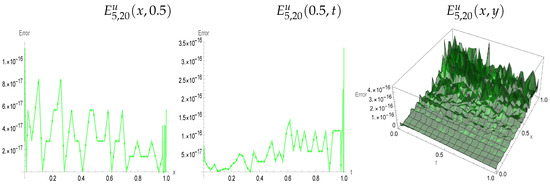
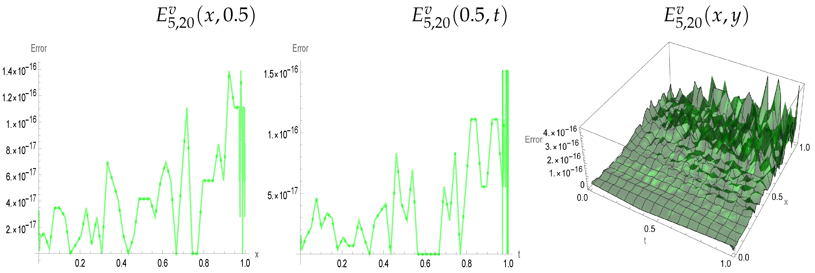
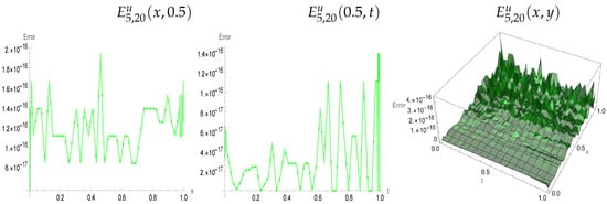
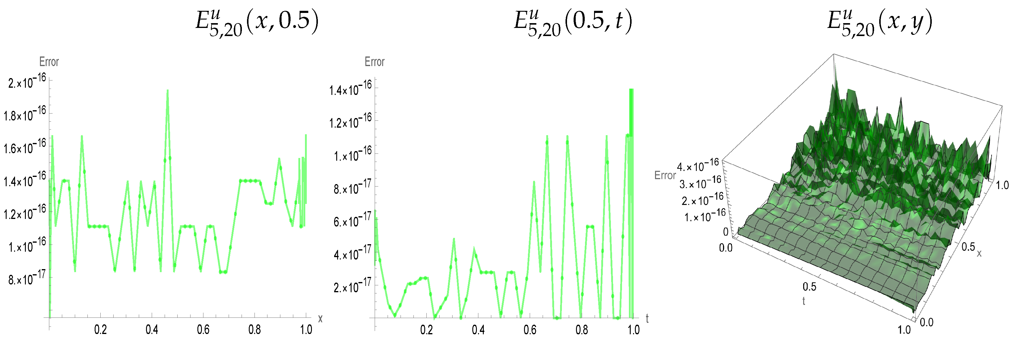
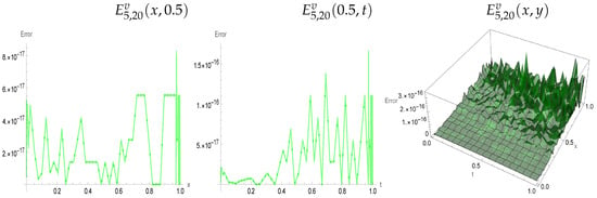
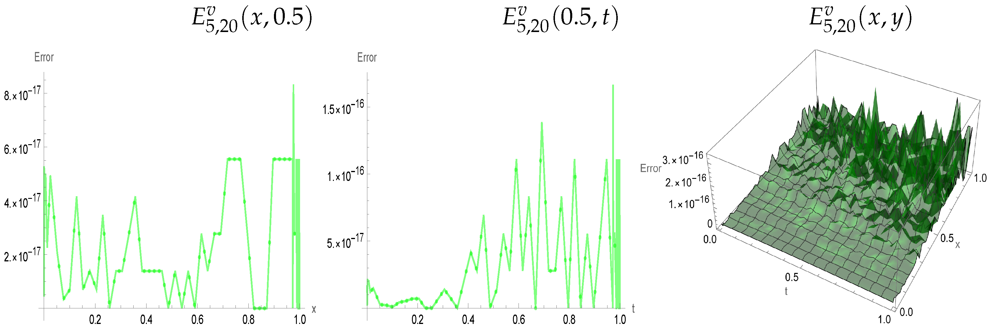
When considering models (5) and (6) with $d_1=d_2=\beta =ϵ=\gamma =1,$${\mu }_1\left(x\right)={\mu }_2\left(x\right)=0,$ and the exact solution is $\left(u(x,t),v(x,t)\right)=\left(t^2{e}^{-x},t^{2}Log(1+x)\right)$, then $f_1(x,t),f_2(x,t)$ are defined accordingly. We test the accuracy of the numerical approach by finding the numerical solution at $Q=5$ and $\sigma =\{0.4,0.5\}.$ This is denoted by $E_{Q,R}^u(x,t)$ and $E_{Q,R}^v(x,t)$, with absolute errors of $|u(x,t)-u_{Q,R}(x,t)|$ and $|v(x,t)-v_{Q,R}(x,t)|$, respectively. Table 1 lists the maximum $E_{5,R}^u(x,t)$ and $E_{5,R}^v(x,t),$ respectively, achieved at $\sigma =\{0.4,0.5\},$ and $R=\{5,10,15,20\}.$ Figure 1 and Figure 2 display the temporal and spatial $E_{5,20}^u(x,t)$ and $E_{5,20}^v(x,t),$ respectively, at $\sigma =0.4$. Figure 3 and Figure 4 display the temporal and spatial $E_{5,20}^u(x,t)$ and $E_{5,20}^v(x,t),$ respectively, at $\sigma =0.5$.

Table 1. Maximum absolute errors with $Q=5$ for Example 2.

	$\mathit{\sigma }=0.4$		$\mathit{\sigma }=0.5$
$\mathit{R}$	$\mathit{u}(\mathit{x},\mathit{t})$	$\mathit{v}(\mathit{x},\mathit{t})$	$\mathit{u}(\mathit{x},\mathit{t})$	$\mathit{v}(\mathit{x},\mathit{t})$
5	$2.5489\times {10}^{-6}$	$2.9831\times {10}^{-5}$	$2.5042\times {10}^{-6}$	$2.9761\times {10}^{-5}$
10	$5.9580\times {10}^{-11}$	$1.8833\times {10}^{-9}$	$5.8572\times {10}^{-11}$	$1.8778\times {10}^{-9}$
15	$1.3655\times {10}^{-14}$	$2.4602\times {10}^{-13}$	$1.3211\times {10}^{-14}$	$2.4556\times {10}^{-13}$
20	$3.3306\times {10}^{-16}$	$3.3306\times {10}^{-16}$	$3.3306\times {10}^{-16}$	$2.2204\times {10}^{-16}$

Figure 1. Absolute errors of $u(x,t)$ at $\sigma =0.4$ and $R=20$ for Example 2.

Figure 2. Absolute errors of $v(x,t)$ at $\sigma =0.4$ and $R=20$ for Example 2.

Figure 3. Absolute errors of $u(x,t)$ at $\sigma =0.5$ and $R=20$ for Example 2.

Figure 4. Absolute errors of $v(x,t)$ at $\sigma =0.5$ and $R=20$ for Example 2.

Remark 1. 

To examine the numerical stability of the proposed method, we performed a perturbation sensitivity test by introducing a controlled small perturbation into the source term of Example 2. The perturbed problem was then solved using the same numerical scheme, and the resulting maximum absolute errors were compared for different perturbation sizes.

As shown in Table 2, the maximum absolute errors increase approximately linearly with the perturbation size. This indicates that small perturbations in the source term lead to proportionally small changes in the numerical solution. This linear behavior demonstrates the stability and robustness of the presented scheme against small perturbations in the source term.

Table 2. Maximum absolute errors for the perturbed problem of Example 2.

	$\mathit{u}(\mathit{x},\mathit{t})$			$\mathit{v}(\mathit{x},\mathit{t})$
$\mathcal{R}$	${\mathit{ϵ}}_{\mathit{s}}=\mathbf{0}.\mathbf{01}$	${\mathit{ϵ}}_{\mathit{s}}=\mathbf{0}.\mathbf{0001}$	${\mathit{ϵ}}_{\mathit{s}}=\mathbf{0}.\mathbf{000001}$	${\mathit{ϵ}}_{\mathit{s}}=\mathbf{0}.\mathbf{01}$	${\mathit{ϵ}}_{\mathit{s}}=\mathbf{0}.\mathbf{0001}$	${\mathit{ϵ}}_{\mathit{s}}=\mathbf{0}.\mathbf{000001}$
5	0.00109421	0.00001342	$2.6134\times {10}^{-6}$	0.00115272	0.00002549	$2.9719\times {10}^{-5}$
10	0.00109188	0.00001091	$1.0923\times {10}^{-7}$	0.00117193	0.00001171	$1.1675\times {10}^{-7}$
20	0.00109188	0.00001091	$1.0918\times {10}^{-7}$	0.00117193	0.00001171	$1.1719\times {10}^{-7}$

Example 3. 

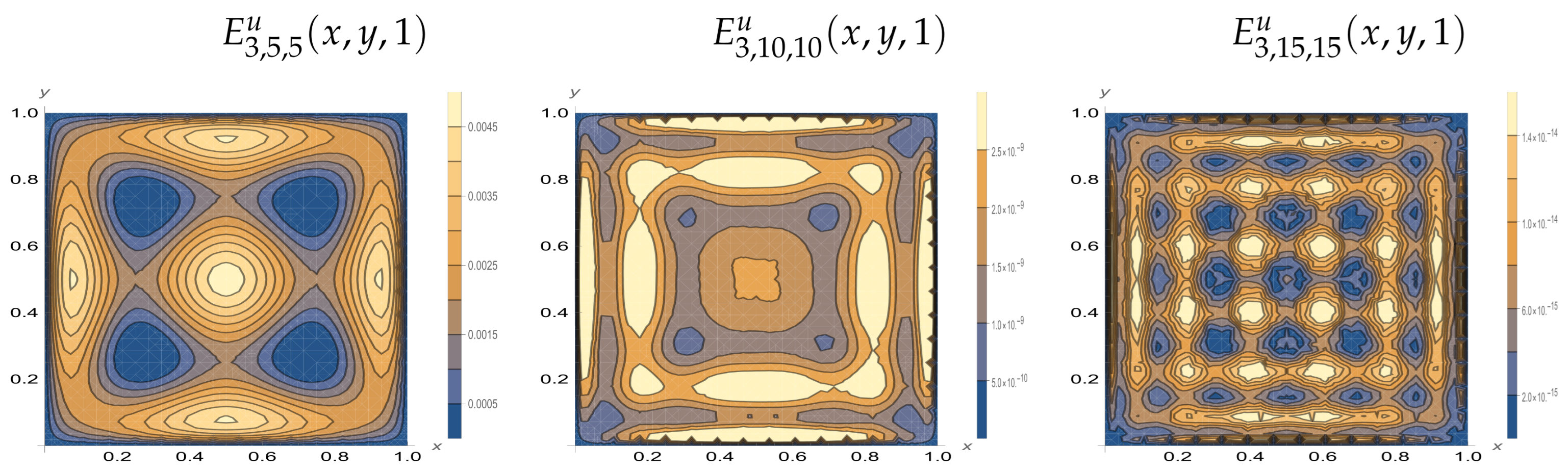
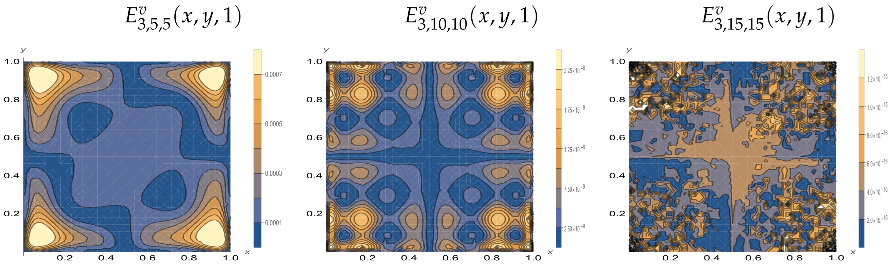
To test the accuracy of the proposed numerical technique to a 2 + 1 model, we consider (12) and (13) with $d_1=d_2=\beta =ϵ=\gamma =1,$${\mu }_1\left(x\right)={\mu }_2\left(x\right)=0,$ and the exact solution is $\left(u(x,t),v(x,t)\right)=\left((t^{\sigma }+t^{2\sigma }+t^{3\sigma })sin\left(\pi x\right)sin\left(\pi y\right),-(t^{\sigma }+t^{2\sigma })cos\left(\pi x\right)cos\left(\pi y\right)\right),$ with $f_1(x,y,t),f_2(x,y,t)$ defined accordingly. We apply the numerical technique introduced in Section 4 with $Q=3$ and different values of R and S. This is denoted by $E_{Q,R,S}^u(x,y,t)$ and $E_{Q,R,S}^v(x,y,t)$, with absolute errors of $|u(x,y,t)-u_{Q,R,S}(x,y,t)|$ and $|v(x,y,t)-v_{Q,R,S}(x,y,t)|$, respectively. Table 3 displays the maximum $E_{3,R,S}^u(x,y,t)$ and $E_{3,R,S}^v(x,y,t)$, respectively, achieved at $\sigma =\{0.25,0.5,0.75\},$ and $R=S=\{4,8,12,16\}.$ Figure 5 and Figure 6 display a contour plot of $E_{3,R,S}^u(x,y,t)$ and $E_{3,R,S}^v(x,y,t)$, respectively, at $\sigma =0.6$ and $R=S=\{5,10,15\}.$

Table 3. Maximum absolute errors with $Q=4$ for Example 3.

	$\mathit{\sigma }=0.25$		$\mathit{\sigma }=0.5$		$\mathit{\sigma }=0.75$
$\mathit{R}=\mathit{S}$	$\mathit{u}(\mathit{x},\mathit{y},\mathit{t})$	$\mathit{v}(\mathit{x},\mathit{y},\mathit{t})$	$\mathit{u}(\mathit{x},\mathit{y},\mathit{t})$	$\mathit{v}(\mathit{x},\mathit{y},\mathit{t})$	$\mathit{u}(\mathit{x},\mathit{y},\mathit{t})$	$\mathit{v}(\mathit{x},\mathit{y},\mathit{t})$
4	$1.02\times {10}^{-2}$	$2.61\times {10}^{-2}$	$1.02\times {10}^{-2}$	$2.61\times {10}^{-2}$	$1.02\times {10}^{-2}$	$2.61\times {10}^{-2}$
8	$6.08\times {10}^{-7}$	$1.75\times {10}^{-6}$	$6.07\times {10}^{-7}$	$1.75\times {10}^{-6}$	$6.05\times {10}^{-7}$	$1.75\times {10}^{-6}$
12	$9.43\times {10}^{-12}$	$6.02\times {10}^{-11}$	$9.42\times {10}^{-12}$	$6.02\times {10}^{-11}$	$9.39\times {10}^{-12}$	$3.02\times {10}^{-11}$
16	$2.22\times {10}^{-15}$	$1.99\times {10}^{-15}$	$2.66\times {10}^{-15}$	$1.55\times {10}^{-15}$	$2.66\times {10}^{-15}$	$1.33\times {10}^{-15}$

Figure 5. Contour plot of absolute errors of $u(x,y,1)$ at $\sigma =0.6$ for Example 3.

Figure 6. Contour plot of absolute errors of $v(x,y,1)$ at $\sigma =0.6$ for Example 3.

6. Conclusions

In this work, we have established a novel set of basis functions, time-nonsmooth and spatially smooth, called the shifted orthogonal Chebyshev function, which formed the basis for a numerical scheme for solving one- and two-dimensional time-fractional FitzHugh–Nagumo models. Based on these new basis, we derived new operational matrices for second-order and fractional-order derivatives in the spatial and time directions, respectively. These new operational matrices coupled with the spectral collocation approach have been implemented to reduce the time-fractional FitzHugh–Nagumo model to a system of algebraic equations. The weak regularity of the new basis near initial time improved the performance of the operational matrices when applied to fractional differential equations. As far as we know, this paper has presented the first use of shifted Chebyshev orthogonal functions to solve time-fractional FitzHugh–Nagumo models, and also the first formulation of operational matrices used. The numerical results have confirmed the high efficiency of using the shifted Chebyshev orthogonal function-based operational matrices for solving time-fractional partial differential equations. The present approach is naturally restricted to rectangular domains due to the use of tensor-product spectral basis functions. Extending the method to irregular domains would require additional techniques, such as coordinate transformations or spectral element methods, which may be considered in future work. In addition, full theoretical stability and convergence analysis remains an important direction for future work.

References

- FitzHugh, R. Impulses and physiological states in theoretical models of nerve membrane. Biophys. J. 1961, 16, 445–466. [Google Scholar] [CrossRef] [Scilit]
- Nagumo, J.; Arimoto, S.; Yoshizawa, S. An Active Pulse Transmission Line Simulating Nerve Axon. Proc. IRE 1962, 50, 2061–2070. [Google Scholar] [CrossRef] [Scilit]
- Yanagida, E. Stability of fast travelling pulse solutions of the FitzHugh-Nagumo equations. J. Math. Biol. 1985, 22, 81–104. [Google Scholar] [CrossRef] [Scilit]
- Krupa, M.; Sandstede, B.; Szmolyan, P. Fast and slow waves in the FitzHugh Nagumo equation. J. Diff. Equ. 1997, 133, 49–97. [Google Scholar] [CrossRef] [Scilit]
- Alfaro, M.; Hilhorst, D.; Matano, H. The singular limit of the Allen-Cahn equation and the FitzHugh-Nagumo system. J. Diff. Equ. 2008, 245, 505–565. [Google Scholar] [CrossRef] [Scilit]
- Pikovsky, A.S.; Kurths, J. Coherence resonance in a noise-driven excitable system. Phys. Rev. Lett. 1997, 78, 775. [Google Scholar] [CrossRef] [Scilit]
- Makarov, V.A.; Nekorkin, V.I.; Velarde, M.G. Spiking behavior in a noise-driven system combining oscillatory and excitatory properties. Phys. Rev. Lett. 2001, 86, 3431. [Google Scholar] [CrossRef] [Scilit] [PubMed]
- Lindner, B.; Ojalvo, J.G.; Neiman, A.; Geier, L.S. Effects of noise in excitable systems. Phys. Rep. 2004, 392, 321–424. [Google Scholar] [CrossRef] [Scilit]
- Bendoukha, S.; Abdelmalek, S.; Kirane, M. Spiral-generation mechanism in the two-dimensional FitzHugh-Nagumo system. Nonlinear Anal. Real World Appl. 2020, 53, 103052. [Google Scholar] [CrossRef] [Scilit]
- Hamadneh, T.; Hioual, A.; Alsayyed, O.; Al-Khassawneh, Y.A.; Al-Husban, A.; Ouannas, A. The FitzHugh-Nagumo Model Described by Fractional Difference Equations: Stability and Numerical Simulation. Axioms 2023, 12, 806. [Google Scholar] [CrossRef] [Scilit]
- Rahby, A.S.; Yang, Z. Asymptotic analysis for time fractional FitzHugh-Nagumo equations. J. Appl. Math. Comput. 2025, 71, 3509–3532. [Google Scholar] [CrossRef] [Scilit]
- Ibrahim, M.M.; Kamran, M.A.; Mannan, M.M.N.; Jung, H.; Kim, S. Lag synchronization of coupled time-delayed FitzHugh-Nagumo neural networks via feedback control. Sci. Rep. 2021, 11, 3884. [Google Scholar] [CrossRef] [Scilit] [PubMed]
- Qu, H.; Zhou, J. Ergodic dynamics of time-fractional FitzHugh-Nagumo diffusive systems with time delays. Neurocomputing 2026, 670, 132455. [Google Scholar] [CrossRef] [Scilit]
- Huang, X.; Yang, H.; Wang, X. Synchronization for fractional FitzHugh-Nagumo equations with fractional Brownian motion. Math. Meth. Appl. Sci. 2023, 46, 517–530. [Google Scholar] [CrossRef] [Scilit]
- Injrou, S.; Mahmoud, S.; Kassem, A. A Stable Numerical Scheme for Fitzhugh-Nagumo Time-Fractional Partial Differential Equation. Tishreen Univ. J. Res. Sci. Stud. Basic Sci. Ser. 2019, 14, 9142. [Google Scholar]
- Karaman, B. On fractional FitzHugh-Nagumo equation as a transmission of nerve impulses design. Int. J. Appl. Comput. Math. 2022, 8, 95. [Google Scholar] [CrossRef] [Scilit]
- Dhumal, M.; Sontakke, B. Solving time-fractional Fitzhugh-Nagumo equation using homotopy perturbation method. Indian J. Sci. Technol. 2024, 17, 1272–1282. [Google Scholar] [CrossRef] [Scilit]
- Cai, L.; Cao, J.; Jing, F.; Wang, Y. A fast time integral finite difference method for a space-time fractional FitzHugh-Nagumo monodomain model in irregular domains. J. Comput. Phys. 2024, 501, 112744. [Google Scholar] [CrossRef] [Scilit]
- Long, C.; Liu, Z.; Ma, C. Synchronization dynamics in fractional-order FitzHugh-Nagumo neural networks with time-delayed coupling. AIMS Math. 2025, 10, 8673–8687. [Google Scholar] [CrossRef] [Scilit]
- Nasir, M.; Yang, S.; Alqudah, M.; Mahnashi, A.M.; Shah, R. Approximate solution of fractional-order FitzHugh-Nagumo equation with in natural transform. J. Appl. Anal. Comput. 2025, 15, 624–639. [Google Scholar] [CrossRef] [Scilit]
- Sahoo, S.; Saha, S.R. On the conservation laws and invariant analysis for time-fractional coupled Fitzhugh-Nagumo equations using the Lie symmetry analysis. Eur. Phys. J. Plus 2019, 134, 83. [Google Scholar] [CrossRef] [Scilit]
- Ezz-Eldien, S.S.; Doha, E.H.; Wang, Y.; Cai, W. A numerical treatment of the two-dimensional multi-term time-fractional mixed sub-diffusion and diffusion-wave equation. Commun. Nonlinear Sci. Numer. Simul. 2020, 91, 105445. [Google Scholar] [CrossRef] [Scilit]
- Ezz-Eldien, S.S.; Alalyani, A. Legendre spectral collocation method for one-and two-dimensional nonlinear pantograph Volterra-Fredholm integro-differential equations. Inter. J. Mod. Phys. C 2025, 37, 255006. [Google Scholar] [CrossRef] [Scilit]
- Wang, Y.; Ezz-Eldien, S.S.; Aldraiweesh, A.A. A new algorithm for the solution of nonlinear two-dimensional Volterra integro-differential equations of high-order. J. Comput. Appl. Math. 2020, 364, 112301. [Google Scholar] [CrossRef] [Scilit]
- Ezz-Eldien, S.S.; Alharbi, W.; Alzubaidi, M.M.; Zaky, M.A. Fractional Chebyshev spectral scheme for time-fractional seventh-order KdV equations with non-smooth solutions. Rom. Rep. Phys. 2026, 78, 104. [Google Scholar] [CrossRef] [Scilit]
- Doha, E.H. Explicit formulae for the coefficients of integrated expansions of Jacobi polynomials and their integrals. Integr. Transforms Spec. Funct. 2003, 14, 69–86. [Google Scholar] [CrossRef] [Scilit]
Disclaimer/Publisher’s Note: The statements, opinions and data contained in all publications are solely those of the individual author(s) and contributor(s) and not of MDPI and/or the editor(s). MDPI and/or the editor(s) disclaim responsibility for any injury to people or property resulting from any ideas, methods, instructions or products referred to in the content. |
© 2026 by the authors. Licensee MDPI, Basel, Switzerland. This article is an open access article distributed under the terms and conditions of the Creative Commons Attribution (CC BY) license.