Local Existence and Regularity of Mild Solutions for Hadamard Fractional Semilinear Integro-Differential Equations with Compact Semigroups

Abstract

We investigate the local well-posedness of semilinear fractional integro-differential equations in Banach spaces with the Hadamard fractional derivative. The equation is ${}^{H}D_t^{\beta }u\left(t\right)=Au\left(t\right)+\phi \left(t,u\left(t\right),{\int }_1^{t}K(t,s)\rho (s,u\left(s\right))ds\right),u\left(1\right)=u_0,$ where A generates a compact $C_0$ semigroup. Using Schauder’s fixed point theorem, we prove local existence under linear growth conditions. Uniqueness is obtained via Banach’s contraction principle under Lipschitz assumptions. The main contribution is a detailed theorem for non-Lipschitz nonlinearities satisfying Carathéodory conditions and Osgood-type growth, where we prove the existence and additional regularity of mild solutions. An illustrative example with Lipschitz nonlinearities is provided.

1. Introduction and Preliminaries

Fractional calculus has recently undergone tremendous development and has become a powerful mathematical tool for modeling physical, biological, and engineering phenomena characterized by memory and hereditary properties. Unlike classical derivatives that depend only on local behavior, fractional derivatives capture the dependence on the past state of the system, making them ideal for describing anomalous diffusion processes, viscoelastic systems, heat transfer in heterogeneous materials, and population dynamics with resting periods. Among the many definitions of fractional derivatives (such as Riemann-Liouville, Caputo, and Grünwald–Letnikov), the Hadamard fractional derivative [1,2,3] stands out due to its unique logarithmic kernel. This kernel makes it particularly suitable for problems defined on intervals starting at $t>1$ and for systems where the influence of the past decays slowly, because the logarithmic transformation allows modeling phenomena with varying time scales.

Fractional integro-differential equations combine the properties of fractional differential equations and integral equations, providing a flexible framework for describing systems in which the instantaneous rates depend on the entire history of the variables. This paper focuses on the local existence and regularity for the equation

$${}^{H}D_t^{\beta }u\left(t\right)=Au\left(t\right)+\phi \left(t,u\left(t\right),{\int }_1^{t}K(t,s)\rho (s,u\left(s\right))ds\right),u\left(1\right)=u_0,$$

(1)

When a compact $C_0$ semigroup is generated by A and

• The infinitesimal generator of a compact $C_0$ semigroup ${\left\{T\left(t\right)\right\}}_{t\ge 1}$ on X is represented by $A:D\left(A\right)\subset X\to X$;
• The continuous nonlinear functions are $\rho ,\phi :J\times X\to X$;
• The continuous kernel is $K:J\times J\to \mathbb{R}$;
• The Hadamard fractional derivative of order $\beta \in (0,1)$ is denoted by ${}^{H}D_t^{\beta }$.

When $\beta =1$, Equation (1) reduces to a classical semilinear integro-differential equation of the type studied by Bahuguna and Srivastava [4] using compact semigroup theory. However, the Hadamard fractional version remains relatively underexplored, despite its wide application potential. The main difficulty lies in the logarithmic kernel, which makes standard techniques (e.g., Laplace transforms) less effective, and in the singular behavior of fractional integrals at the initial point $t=1$. Moreover, the presence of the nonlinear integral term further complicates the analysis.

Several works have used fixed-point theory to study the existence and uniqueness of fractional differential equations. For example, Li and Changpin [5] applied Banach’s contraction principle in Hölder spaces. On the other hand, Zhou, Li and Zhou [6] relied on Schauder’s theorem for the existence of mild solutions to fractional evolution equations with nonlocal boundary conditions. However, most of these studies assumed that the nonlinear functions satisfy a Lipschitz condition, which is a restrictive requirement in many practical applications where functions may exhibit behavior such as $u\log (1+|u\left|\right)$ or non-Lipschitz integral dependencies. Such cases require more delicate treatment using Carathéodory conditions and Osgood-type growth.

The main contribution of this paper is providing a local existence and regularity theorem for mild solutions without assuming the Lipschitz continuity of the nonlinearities. Instead, we use Carathéodory conditions (see [7], standard in ordinary differential equations) together with integral growth conditions (see [8,9]) that allow functions such as $u\log (1+|u\left|\right)$ or higher powers. The compactness of the semigroup generated by $-A$ compensates for the lack of Lipschitz continuity, allowing the application of Schauder’s fixed-point theorem in the space of continuous functions. We also prove that if the initial value $u_0$ belongs to the domain $D\left(A\right)$ of the generator, then the mild solution gains additional regularity (belongs to Hölder space $C^{\gamma }$).

Given the importance of Hadamard fractional integro-differential equations in engineering and physics applications (see [10,11,12,13]), these results provide new theoretical tools for analyzing such systems. Furthermore, the illustrative example presented in Section 4 on the $L^2\left([0,\pi ]\right)$ space verifies the required conditions and shows how the theorems can be applied in a practical context.

The present work also demonstrates how different techniques can be combined: compact semigroup theory, Hadamard fractional integrals, fixed-point theorems (Schauder, Banach), Hölder inequalities, and logarithmic kernel estimates. This combination has not been used systematically in previous studies for the Hadamard integro-differential equation.

In Section 2 we recall the necessary definitions and preliminaries (Hadamard fractional integral, derivative, compact semigroup, mild solution, and Hadamard–Gronwall inequality). Section 3 is devoted to local existence results: first using Schauder under linear growth conditions (Theorem 1), then using Banach under Lipschitz assumptions to obtain uniqueness (Theorem 2). Section 4 contains the main theoretical contribution (Theorem 3), where we treat non-Lipschitz nonlinearities satisfying Carathéodory conditions and integral growth, and we prove existence together with additional regularity. In Section 6 we present a detailed example on $L^2\left([0,\pi ]\right)$ with the Laplace operator and Dirichlet boundary conditions, showing how the conditions of Banach’s theorem are satisfied. We conclude this paper with a discussion of the results and future research directions.

Fractional differential equations have become essential tools for modeling memory and hereditary phenomena in various fields of science and engineering.

Let X be a Banach space with norm $∥·∥$. For $T>1$, set $J=[1,T]$. Let $C(J,X)$ denote the space of continuous functions with the supremum norm ${∥u∥}_{\infty }={sup}_{t\in J}∥u\left(t\right)∥$.

Definition 1 

([1]). For $\beta >0$ and a function $\phi :[1,\infty )\to X$, the Hadamard fractional integral of order β is

$$I^{\beta }\phi \left(t\right)={\displaystyle \frac{1}{\Gamma \left(\beta \right)}}{\int }_1^t{\left(\log {\displaystyle \frac{t}{s}}\right)}^{\beta -1}\phi \left(s\right){\displaystyle \frac{ds}{s}},$$

provided the integral exists.

Definition 2 

([1]). For $\beta \in (0,1)$ and $\phi :[1,\infty )\to X$, the Hadamard fractional derivative of order β is

$${}^{H}D^{\beta }\phi \left(t\right)={\displaystyle \frac{1}{\Gamma (1-\beta )}}\left(t{\displaystyle \frac{d}{dt}}\right){\int }_1^t{\left(\log {\displaystyle \frac{t}{s}}\right)}^{-\beta }\phi \left(s\right){\displaystyle \frac{ds}{s}}.$$

Remark 1. 

The Hadamard derivative is defined on intervals $[a, M]$ with $a>0$ because the kernel involves $\log (s/\tau )$ and requires $s,\tau >0$. In this paper we take $a=1$ for simplicity. This choice is not restrictive: any initial value problem given on $[0, M]$ can be transformed to $[1, M+1]$ by a translation $s\mapsto s+1$, which preserves the constant delay γ. Hence the domain $[1, M]$ is without loss of generality.

Definition 3 

($C_0$ semigroup [14]). A family ${\left\{T\left(t\right)\right\}}_{t\ge 1}\subset \mathcal{L}\left(X\right)$ is a $C_0$ semigroup if:

• $T(t+s)=T\left(t\right)T\left(s\right)$$\forall t,s\ge 1$;
• $T\left(1\right)=I$;
• ${lim}_{t\to 1^{+}}T\left(t\right)x=x$ for every $x\in X$.

$Ax={lim}_{t\to 1^{+}}{\displaystyle \frac{T\left(t\right)x-x}{t}}$ with domain $D\left(A\right)=\{x\in X:Ax\mathit{exists}\}$ defines the infinitesimal generator A.

Definition 4 

([14]). A $C_0$ semigroup ${\left\{T\left(t\right)\right\}}_{t\ge 1}$ is called compact if $T\left(t\right)$ is a compact operator for every $t>1$.

Remark 2. 

Throughout this paper, we assume that $-A$ generates a compact $C_0$ semigroup ${\left\{T\left(t\right)\right\}}_{t\ge 1}$. Compactness is essential for applying Schauder’s fixed-point theorem and for obtaining regularity. Note that the semigroup is defined for $t\ge 1$, while the fractional integral starts at 1; this is not a conflict because we evaluate $T(t-s)$ for $t\ge s\ge 1$, so $t-s\ge 0$.

Definition 5 

(Mild solution). If a function $u\in C(J,X)$ fulfills the integral equation, it is referred to be a mild solution of (1).

$$u\left(t\right)=T(t-1)u_0+{\displaystyle \frac{1}{\Gamma \left(\beta \right)}}{\int }_1^t{\left(\log {\displaystyle \frac{t}{s}}\right)}^{\beta -1}T(t-s)F\left(u\right)\left(s\right){\displaystyle \frac{ds}{s}},$$

(2)

where

$$F\left(u\right)\left(s\right)=\phi \left(s,u\left(s\right),{\int }_1^{s}K(s,\tau )\rho (\tau ,u\left(\tau \right))d\tau \right).$$

Lemma 1 

(Hadamard–Gronwall [15]). Let $\beta >0$, and let $u\left(t\right),v\left(t\right)$ be non-negative locally integrable functions on $[1,T]$. Assume that $M\left(t\right)$ is non-negative, nondecreasing, and bounded by a constant m. If

$$u\left(t\right)\le v\left(t\right)+M\left(t\right){\int }_1^t{\left(\log {\displaystyle \frac{t}{s}}\right)}^{\beta -1}u\left(s\right){\displaystyle \frac{ds}{s}},$$

then

$$u\left(t\right)\le v\left(t\right)+{\int }_1^t\left[{\displaystyle \sum _{k=1}^{\infty }}{\displaystyle \frac{{(M\left(t\right)\Gamma \left(\beta \right))}^k}{\Gamma \left(k\beta \right)}}{\left(\log {\displaystyle \frac{t}{s}}\right)}^{k\beta -1}v\left(s\right)\right]{\displaystyle \frac{ds}{s}}.$$

In particular, if $v\left(t\right)\equiv a$ (constant), then $u\left(t\right)\le a{E}_{\beta }\left(m\Gamma \left(\beta \right){\left(\log t\right)}^{\beta }\right)$, where $E_{\beta }$ is the Mittag–Leffler function defined by $E_{\beta }\left(z\right)={\sum }_{k=0}^{\infty }{\displaystyle \frac{z^k}{\Gamma (\beta k+1)}}$.

2. Local Existence via Schauder’s Fixed-Point Theorem

This section establishes many local existence findings for mild solutions to the semilinear fractional integro-differential problem (1). The compactness of the semigroup generated by $-A$ is crucial to our study since it allows us to apply many fixed-point theorems.

Theorem 1. 

Let $-A$ generate a compact $C_0$ semigroup ${\left\{T\left(t\right)\right\}}_{t\ge 1}$ on X satisfying $\parallel T\left(t\right)\parallel \le M$ for all $t\ge 1$. Suppose further:

• The kernel $K:J\times J\to \mathbb{R}$ is continuous, and there exists $K_0>0$ such that $\left|K(t,s)\right|\le K_0$ for every $t,s\in J$;
• The maps $\rho ,\phi :J\times X\to X$ are continuous;
• For every $t\in J$ and every $u,v\in X$, there are positive constants $L_{\phi },L_{\rho }$ such that

  $$\parallel \phi (t,u,v)\parallel \le L_{\phi }(1+\parallel u\parallel +\parallel v\parallel ),\parallel \rho (t,u)\parallel \le L_{\rho }(1+\parallel u\parallel ).$$

Then, for each $u_0\in X$, one can find $T_0\in (1,T]$ such that (1) admits a minimum of one mild solution $u\in C([1,T_0],X)$.

Proof. 

The proof is broken up into steps.

• Step 1:

Define $\mathsf{\Phi }:C([1,T_0],X)\to C([1,T_0],X)$ by

$$\left(\mathsf{\Phi }u\right)\left(t\right)=T(t-1)u_0+{\displaystyle \frac{1}{\Gamma \left(\beta \right)}}{\int }_1^t{\left(\log {\displaystyle \frac{t}{s}}\right)}^{\beta -1}T(t-s)F\left(u\right)\left(s\right){\displaystyle \frac{ds}{s}},$$

where $F\left(u\right)\left(s\right)=\phi \left(s,u\left(s\right),{\int }_1^{s}K(s,\tau )\rho (\tau ,u\left(\tau \right))d\tau \right)$.

Step 2:

Choice of parameters.

Let $R>0$ be a constant to be determined later. Consider the closed ball

$$B_R=\left\{u\in C([1,T_0],X):{∥u∥}_{\infty }\le R\right\}.$$

We will show that, for sufficiently small $T_0>1$ and appropriately chosen R, $\mathsf{\Phi }$ maps $B_R$ into itself.

Take any $u\in B_R$. For $t\in [1,T_0]$, we estimate

$$\begin{array}{cc}\hfill ∥\left(\mathsf{\Phi }u\right)\left(t\right)∥& \le ∥T(t-1)u_0∥+{\displaystyle \frac{1}{\Gamma \left(\beta \right)}}{\int }_1^t{\left(\log {\displaystyle \frac{t}{s}}\right)}^{\beta -1}∥T(t-s)∥\hfill \\ & \times ∥\phi \left(s,u\left(s\right),{\int }_1^{s}K(s,\tau )\rho (\tau ,u\left(\tau \right))d\tau \right)∥{\displaystyle \frac{ds}{s}}.\hfill \end{array}$$

Since $∥T\left(t\right)∥\le M$, we have

$$∥\left(\mathsf{\Phi }u\right)\left(t\right)∥\le M∥u_0∥+{\displaystyle \frac{M}{\Gamma \left(\beta \right)}}{\int }_1^t{\left(\log {\displaystyle \frac{t}{s}}\right)}^{\beta -1}∥\phi (·)∥{\displaystyle \frac{ds}{s}}.$$

Now estimate the argument of $\phi$. Using the growth condition on $\rho$ and the boundedness of K,

$$\begin{array}{cc}\hfill ∥{\int }_1^{s}K(s,\tau )\rho (\tau ,u\left(\tau \right))d\tau ∥& \le {\int }_1^s\left|K(s,\tau )\right|∥\rho (\tau ,u(\tau \left)\right)∥d\tau \hfill \\ & \le K_0{\int }_1^s{L}_{\rho }(1+∥u\left(\tau \right)∥)d\tau \hfill \\ & \le K_0{L}_{\rho }(1+R)(s-1)\hfill \\ & \le K_0{L}_{\rho }(1+R)(T_0-1).\hfill \end{array}$$

Hence, using the growth condition on $\phi$,

$$∥\phi (·)∥\le L_{\phi }\left(1+∥u\left(s\right)∥+K_0{L}_{\rho }(1+R)(T_0-1)\right)\le L_{\phi }\left(1+R+K_0{L}_{\rho }(1+R)(T_0-1)\right).$$

Thus

$$∥\left(\mathsf{\Phi }u\right)\left(t\right)∥\le M∥u_0∥+{\displaystyle \frac{M{L}_{\phi }(1+R)\left(1+K_0{L}_{\rho }(T_0-1)\right)}{\Gamma \left(\beta \right)}}{\int }_1^t{\left(\log {\displaystyle \frac{t}{s}}\right)}^{\beta -1}{\displaystyle \frac{ds}{s}}.$$

Compute the integral:

$${\int }_1^t{\left(\log {\displaystyle \frac{t}{s}}\right)}^{\beta -1}{\displaystyle \frac{ds}{s}}={\int }_0^{\log t}{u}^{\beta -1}du={\displaystyle \frac{{\left(\log t\right)}^{\beta }}{\beta }}\le {\displaystyle \frac{{\left(\log T_0\right)}^{\beta }}{\beta }}.$$

Therefore,

$$∥\left(\mathsf{\Phi }u\right)\left(t\right)∥\le M∥u_0∥+{\displaystyle \frac{M{L}_{\phi }(1+R)\left(1+K_0{L}_{\rho }(T_0-1)\right){\left(\log T_0\right)}^{\beta }}{\beta \Gamma \left(\beta \right)}}.$$

Choose $R=2M∥u_0∥+1$. Then, for $T_0>1$ sufficiently close to 1 (so that $\log T_0$ and $T_0-1$ are small enough), the second term becomes less than $R/2$. Consequently,

$$∥\left(\mathsf{\Phi }u\right)\left(t\right)∥\le {\displaystyle \frac{R}{2}}+{\displaystyle \frac{R}{2}}=R,$$

which shows $\mathsf{\Phi }\left(B_R\right)\subset B_R$.

Step 3:

Continuity of $\mathsf{\Phi }$.

Let $\left\{u_n\right\}$ be a sequence in $B_R$ converging uniformly to $u\in B_R$. Since $\phi ,\rho ,K$ are continuous, we have pointwise convergence:

$$F\left(u_n\right)\left(s\right)\to F\left(u\right)\left(s\right)\mathrm{for}\mathrm{each}s\in [1,T_0].$$

Moreover, from the growth conditions, $F\left(u_n\right)\left(s\right)$ is bounded uniformly in n and s. Thus, the dominated convergence theory implies

$$\underset{t\in [1,T_0]}{sup}∥\left(\mathsf{\Phi }{u}_n\right)\left(t\right)-\left(\mathsf{\Phi }u\right)\left(t\right)∥\to 0\mathrm{as}n\to \infty .$$

Hence $\mathsf{\Phi }$ is continuous.

Step 4:

Compactness of $\mathsf{\Phi }$ (complete continuity).

We show that $\mathsf{\Phi }\left(B_R\right)$ is equicontinuous and relatively compact in $C([1,T_0],X)$.

Equicontinuity: Let $1\le t_1<t_2\le T_0$ and $u\in B_R$. Then

$$\begin{array}{cc}\hfill \left(\mathsf{\Phi }u\right)\left(t_2\right)-\left(\mathsf{\Phi }u\right)\left(t_1\right)& = \left(T(t_2-1)-T(t_1-1)\right)u_0\hfill \\ & + {\displaystyle \frac{1}{\Gamma \left(\beta \right)}}{\int }_1^{t_2}{\left(\log {\displaystyle \frac{t_2}{s}}\right)}^{\beta -1}T(t_2-s)F\left(u\right)\left(s\right){\displaystyle \frac{ds}{s}}\hfill \\ & - {\displaystyle \frac{1}{\Gamma \left(\beta \right)}}{\int }_1^{t_1}{\left(\log {\displaystyle \frac{t_1}{s}}\right)}^{\beta -1}T(t_1-s)F\left(u\right)\left(s\right){\displaystyle \frac{ds}{s}}.\hfill \end{array}$$

The first term tends to 0 as $t_2\to t_1$ because $T\left(t\right)$ is strongly continuous. The difference of the two integrals can be split into three parts:

$$\begin{array}{cc}& {\int }_1^{t_1}\left[{\left(\log {\displaystyle \frac{t_2}{s}}\right)}^{\beta -1}T(t_2-s)-{\left(\log {\displaystyle \frac{t_1}{s}}\right)}^{\beta -1}T(t_1-s)\right]F\left(u\right)\left(s\right){\displaystyle \frac{ds}{s}}\hfill \\ & +{\int }_{t_1}^{t_2}{\left(\log {\displaystyle \frac{t_2}{s}}\right)}^{\beta -1}T(t_2-s)F\left(u\right)\left(s\right){\displaystyle \frac{ds}{s}}.\hfill \end{array}$$

Using the uniform continuity of the kernel $\theta \mapsto {\left(\log \theta \right)}^{\beta -1}$ on compact intervals and the strong continuity of $T(·)$, each part becomes arbitrarily small uniformly in $u\in B_R$ as $t_2-t_1\to 0$. Hence $\mathsf{\Phi }\left(B_R\right)$ is equicontinuous.

For a fixed $t\in (1,T_0]$, consider the set $\{\mathsf{\Phi }u\left(t\right):u\in B_R\}$. We can write

$$\mathsf{\Phi }u\left(t\right)=T(t-1)u_0+{\displaystyle \frac{1}{\Gamma \left(\beta \right)}}\underset{n\to \infty }{lim}{\displaystyle \sum _{i=1}^n}{\left(\log {\displaystyle \frac{t}{s_i}}\right)}^{\beta -1}T(t-s_i)F\left(u\right)\left(s_i\right){\displaystyle \frac{\Delta s_i}{s_i}}$$

as a limit of Riemann sums. Since $T(t-s_i)$ is compact for $t-s_i>0$ and the coefficients are bounded, each Riemann sum lies in a compact set. The limit (uniform in u) therefore lies in the closed convex hull of a compact set, which is compact. Thus $\{\mathsf{\Phi }u\left(t\right):u\in B_R\}$ is relatively compact in X. From Arzelà–Ascoli theorem, $\mathsf{\Phi }\left(B_R\right)$ is relatively compact in $C([1,T_0],X)$.

Step 5:

Application of Schauder’s theorem.

We showed that $\mathsf{\Phi }:B_R\to B_R$ is continuous and completely continuous (maps bounded sets into relatively compact sets). Schauder’s fixed-point theorem guarantees the existence of a fixed point $u\in B_R$ such that $\mathsf{\Phi }u=u$. By definition, this u is a mild solution of (1) on $[1,T_0]$. This completes the proof. □

We derive the following results for local existence and uniqueness using Banach contraction:

Theorem 2. 

Let $-A$ generate be a compact $C_0$ semigroup ${\left\{T\left(t\right)\right\}}_{t\ge 1}$ on X with $\parallel T\left(t\right)\parallel \le M$ for all $t\ge 1$. Assume the subsequent circumstances are met:

• The kernel $K:J\times J\to \mathbb{R}$ is continuous and satisfies $\left|K(t,s)\right|\le K_0$ for some constant $K_0>0$;
• The functions $\rho ,\phi :J\times X\to X$ are continuous;
• For every $t\in J$ and every $u_1,u_2,v_1,v_2\in X$, there are constants $L_{\phi },L_{\rho }>0$ such that

  $$\begin{array}{cc}\hfill \parallel \phi (t,u_1,v_1)-\phi (t,u_2,v_2)\parallel & \le L_{\phi }\left(\parallel u_1-u_2\parallel + \parallel v_1-v_2\parallel \right),\hfill \\ \hfill \parallel \rho (t,u_1)-\rho (t,u_2)\parallel & \le L_{\rho }\parallel u_1-u_2\parallel .\hfill \end{array}$$

Then, for each initial value $u_0\in X$, there exists $T_0>1$ such that (1) possesses a unique mild solution $u\in C([1,T_0],X)$.

Proof. 

Define the operator $\mathsf{\Phi }$ as in the previous proof. For any $u,v\in C\left(\right[1,T],X)$, we estimate the difference.

Step 1:

Lipschitz estimate for F.

Let $I_1\left(u\right)\left(s\right)={\int }_1^{s}K(s,\tau )\rho (\tau ,u\left(\tau \right))d\tau$. Then

$$\begin{array}{cc}\hfill ∥I_1\left(u\right)\left(s\right)-I_1\left(v\right)\left(s\right)∥& \le {\int }_1^s\left|K(s,\tau )\right|∥\rho (\tau ,u(\tau \left)\right)-\rho (\tau ,v(\tau \left)\right)∥d\tau \hfill \\ & \le K_0{L}_{\rho }{\int }_1^s∥u\left(\tau \right)-v\left(\tau \right)∥d\tau .\hfill \end{array}$$

Using the Lipschitz property of $\phi$,

$$\begin{array}{cc}& ∥F\left(u\right)\left(s\right)-F\left(v\right)\left(s\right)∥\hfill \\ & \le L_{\phi }\left(∥u\left(s\right)-v\left(s\right)∥+∥I_1\left(u\right)\left(s\right)-I_1\left(v\right)\left(s\right)∥\right)\hfill \\ & \le L_{\phi }∥u\left(s\right)-v\left(s\right)∥+L_{\phi }{K}_0{L}_{\rho }{\int }_1^s∥u\left(\tau \right)-v\left(\tau \right)∥d\tau .\hfill \end{array}$$

Step 2:

Estimate for $\mathsf{\Phi }u-\mathsf{\Phi }v$.

$$\begin{array}{cc}\hfill ∥\left(\mathsf{\Phi }u\right)\left(t\right)-\left(\mathsf{\Phi }v\right)\left(t\right)∥& \le {\displaystyle \frac{M}{\Gamma \left(\beta \right)}}{\int }_1^t{\left(\log {\displaystyle \frac{t}{s}}\right)}^{\beta -1}∥F\left(u\right)\left(s\right)-F\left(v\right)\left(s\right)∥{\displaystyle \frac{ds}{s}}\hfill \\ & \le {\displaystyle \frac{M{L}_{\phi }}{\Gamma \left(\beta \right)}}{\int }_1^t{\left(\log {\displaystyle \frac{t}{s}}\right)}^{\beta -1}∥u\left(s\right)-v\left(s\right)∥{\displaystyle \frac{ds}{s}}\hfill \\ & + {\displaystyle \frac{M{L}_{\phi }{K}_0{L}_{\rho }}{\Gamma \left(\beta \right)}}{\int }_1^t{\left(\log {\displaystyle \frac{t}{s}}\right)}^{\beta -1}{\int }_1^s∥u\left(\tau \right)-v\left(\tau \right)∥d\tau {\displaystyle \frac{ds}{s}}.\hfill \end{array}$$

Step 3:

Simplify the double integral.

Let $\psi \left(t\right)={sup}_{1\le \tau \le t}∥u\left(\tau \right)-v\left(\tau \right)∥$. Then

$${\int }_1^t{\left(\log {\displaystyle \frac{t}{s}}\right)}^{\beta -1}∥u\left(s\right)-v\left(s\right)∥{\displaystyle \frac{ds}{s}}\le \psi \left(t\right){\displaystyle \frac{{\left(\log t\right)}^{\beta }}{\beta }}.$$

For the double integral, swap the order of integration:

$$\begin{array}{cc}\hfill {\int }_1^t{\left(\log {\displaystyle \frac{t}{s}}\right)}^{\beta -1}{\int }_1^s∥u\left(\tau \right)-v\left(\tau \right)∥d\tau {\displaystyle \frac{ds}{s}}& = {\int }_1^t∥u\left(\tau \right)-v\left(\tau \right)∥{\int }_{\tau }^t{\left(\log {\displaystyle \frac{t}{s}}\right)}^{\beta -1}{\displaystyle \frac{ds}{s}}d\tau \hfill \\ & = {\int }_1^t∥u\left(\tau \right)-v\left(\tau \right)∥{\displaystyle \frac{{\left(\log (t/\tau )\right)}^{\beta }}{\beta }}d\tau \hfill \\ & \le \psi \left(t\right){\displaystyle \frac{{\left(\log t\right)}^{\beta +1}}{\beta (\beta +1)}}.\hfill \end{array}$$

Step 4:

Contraction condition.

Combining the estimates, we obtain

$$∥\left(\mathsf{\Phi }u\right)\left(t\right)-\left(\mathsf{\Phi }v\right)\left(t\right)∥\le \psi \left(t\right)\left({\displaystyle \frac{M{L}_{\phi }{\left(\log T\right)}^{\beta }}{\beta \Gamma \left(\beta \right)}}+{\displaystyle \frac{M{L}_{\phi }{K}_0{L}_{\rho }{\left(\log T\right)}^{\beta +1}}{\beta (\beta +1)\Gamma \left(\beta \right)}}\right).$$

Choose $T_0>1$ so small that

$${\displaystyle \frac{M{L}_{\phi }{\left(\log T_0\right)}^{\beta }}{\beta \Gamma \left(\beta \right)}}+{\displaystyle \frac{M{L}_{\phi }{K}_0{L}_{\rho }{\left(\log T_0\right)}^{\beta +1}}{\beta (\beta +1)\Gamma \left(\beta \right)}}<1.$$

Consequently, $\mathsf{\Phi }$ is a contraction on $C([1,T_0],X)$. The unique mild solution on $[1,T_0]$ is the unique fixed point of $\mathsf{\Phi }$ according to Banach’s fixed-point theorem. □

3. Existence and Regularity with Non-Lipschitz Nonlinearities

We use the following estimates (proved by elementary calculus):

$${\int }_1^t{\left(\log {\displaystyle \frac{t}{s}}\right)}^{\beta -1}{\displaystyle \frac{ds}{s}}={\displaystyle \frac{{\left(\log t\right)}^{\beta }}{\beta }},{\int }_1^t{\left(\log {\displaystyle \frac{t}{s}}\right)}^{\beta -1}{\displaystyle \frac{ds}{s}}\le {\displaystyle \frac{{\left(\log T\right)}^{\beta }}{\beta }}\mathrm{for}t\le T.$$

For completeness, we recall the standard results (proofs can be found in [4]). The classical local existence and uniqueness results under linear growth conditions (Schauder) and Lipschitz conditions (Banach) were already established in Theorems 1 and 2 in Section 2. Therefore, in this section we focus solely on the more general case with Carathéodory conditions and Osgood-type nonlinearities (Theorem 3 below).

Remark 3. 

The existence of $T_0$ depends on the Lipschitz constants and on the bound of $\parallel \phi (t,0,0)\parallel ,\parallel \rho (t,0,0)\parallel$ through the choice of R and the requirement that $\mathsf{\Phi }\left(B_R\right)\subset B_R$. The contraction condition $\kappa \left(T_0\right)<1$ can be satisfied independently of the size of the initial data by taking $T_0$ sufficiently close to 1. This is standard for semilinear evolution equations with Lipschitz nonlinearities.

This is the main theoretical contribution. We now consider the case where $\phi$ is not necessarily Lipschitz but satisfies Carathéodory conditions and a growth condition that allows for nonlinearities like $u\log (1+|u\left|\right)$.

Theorem 3. 

Suppose $-A$ generates a compact $C_0$ semigroup ${\left\{T\left(t\right)\right\}}_{t\ge 1}$ on X such that $\parallel T\left(t\right)\parallel \le M{e}^{\omega t}$ for some $M\ge 1$ and $\omega \in \mathbb{R}$. The subsequent hypotheses are imposed:

(A) 

The map $\phi :J\times X\times X\to X$ fulfills the Carathéodory conditions:

• For each fixed $u,v\in X$, the function $t\mapsto \phi (t,u,v)$ is measurable;
• For almost every $t\in J$, the mapping $(u,v)\mapsto \phi (t,u,v)$ is continuous;
• There exist a continuous nondecreasing ${\psi }_{\phi }:{\mathbb{R}}^{+}\to {\mathbb{R}}^{+}$ and a function $m_{\phi }\in L^p(J,{\mathbb{R}}^{+})$ with $p>1/\beta$ with

  $$\parallel \phi (t,u,v)\parallel \le m_{\phi }\left(t\right){\psi }_{\phi }(\parallel u\parallel +\parallel v\parallel )\mathit{for}a.e.t\in J,\forall u,v\in X.$$

(B) 

The map $\rho :J\times X\to X$ is completely continuous (i.e., it sends bounded sets to relatively compact ones). Moreover:

• There exist a continuous nondecreasing ${\psi }_{\rho }:{\mathbb{R}}^{+}\to {\mathbb{R}}^{+}$ and an $m_{\rho }\in L^q(J,{\mathbb{R}}^{+})$ with $q>1/\beta$ with

  $$\parallel \rho (t,u)\parallel \le m_{\rho }\left(t\right){\psi }_{\rho }(\parallel u\parallel )\mathit{for}a.e.t\in J,\forall u\in X;$$
• ρ is uniformly continuous on every bounded subset of $J\times X$.

(C) 

The kernel $K:J\times J\to \mathbb{R}$ is bounded and continuous, i.e., $\left|K(t,s)\right|\le K_0$ for some $K_0>0$ and all $t,s\in J$.

(D) 

The subsequent growth requirement is met:

$$\underset{r\to \infty }{lim\; inf}{\displaystyle \frac{{\psi }_{\phi }\left(r\right)+K_0{\psi }_{\rho }\left(r\right)}{r}}<{\displaystyle \frac{\Gamma (\beta +1)}{M{e}^{\omega T}\left(\parallel m_{\phi }{\parallel }_{L^p}+K_0{\parallel m_{\rho }\parallel }_{L^q}\right){\left(\log T\right)}^{\beta }}}.$$

Then, for every initial datum $u_0\in X$, one can find $T_0\in (1,T]$ such that (1) possesses at least one mild solution $u\in C([1,T_0],X)$. Furthermore, if $u_0$ belongs to $D\left(A\right)$ (the domain of the generator), the mild solution shows extra regularity: $u\in C^{\gamma }((1,T_0],X)$ for some $\gamma >0$, and it more strongly fulfills the equation.

Proof. 

The proof is broken up into many steps.

Define $\mathsf{\Phi }:C([1,T_0],X)\to C([1,T_0],X)$ by

$$\left(\mathsf{\Phi }u\right)\left(t\right)=T(t-1)u_0+{\displaystyle \frac{1}{\Gamma \left(\beta \right)}}{\int }_1^t{\left(\log {\displaystyle \frac{t}{s}}\right)}^{\beta -1}T(t-s)F\left(u\right)\left(s\right){\displaystyle \frac{ds}{s}},$$

with $F\left(u\right)\left(s\right)=\phi (s,u\left(s\right),{\int }_1^{s}K(s,\tau )\rho (\tau ,u\left(\tau \right))d\tau )$.

Step 2:

Choice of parameters.

Let $R>0$ be a constant to be fixed later. Set

$$B_R=\{u\in C([1,T_0],X){:\parallel u\parallel }_{\infty }\le R\}.$$

We show that for sufficiently small $T_0>1$ and appropriate R, $\mathsf{\Phi }\left(B_R\right)\subset B_R$, and $\mathsf{\Phi }$ is completely continuous.

First, estimate the inner integral term. For any $u\in B_R$ and $s\in [1,T_0]$,

$$\begin{array}{cc}\hfill ∥{\int }_1^{s}K(s,\tau )\rho (\tau ,u\left(\tau \right))d\tau ∥& \le K_0{\int }_1^s\parallel \rho (\tau ,u\left(\tau \right))\parallel d\tau \hfill \\ & \le K_0{\int }_1^s{m}_{\rho }\left(\tau \right){\psi }_{\rho }(\parallel u\left(\tau \right)\parallel )d\tau \hfill \\ & \le K_0{\psi }_{\rho }\left(R\right){\int }_1^{T_0}{m}_{\rho }\left(\tau \right)d\tau \hfill \\ & \le K_0{\psi }_{\rho }\left(R\right){\parallel m_{\rho }\parallel }_{L^1\left([1,T_0]\right)}.\hfill \end{array}$$

Since $q>1/\beta$, Hölder’s inequality gives $\parallel m_{\rho }{\parallel }_{L^1}\le {(T_0-1)}^{1-1/q}{\parallel m_{\rho }\parallel }_{L^q}$. For small $T_0$, this is small.

Now, using the growth condition on $\phi$,

$$\parallel F\left(u\right)\left(s\right)\parallel \le m_f\left(s\right){\psi }_f\left(R+K_0{\psi }_{\rho }\left(R\right){\parallel m_{\rho }\parallel }_{L^1}\right).$$

Denote $C_R={\psi }_{\phi }\left(R+K_0{\psi }_{\rho }\left(R\right){\parallel m_{\rho }\parallel }_{L^1\left([1,T_0]\right)}\right)$. Then

$$\parallel \left(\mathsf{\Phi }u\right)\left(t\right)\parallel \le M{e}^{\omega (t-1)}\parallel u_0\parallel +{\displaystyle \frac{M{e}^{\omega (T_0-1)}}{\Gamma \left(\beta \right)}}{C}_R{\int }_1^t{\left(\log {\displaystyle \frac{t}{s}}\right)}^{\beta -1}{m}_{\phi }\left(s\right){\displaystyle \frac{ds}{s}}.$$

Utilizing exponents p and $p^{\prime }$ (where $1/p+1/p^{\prime }=1$), apply Hölder’s inequality:

$${\int }_1^t{\left(\log {\displaystyle \frac{t}{s}}\right)}^{\beta -1}{m}_{\phi }\left(s\right){\displaystyle \frac{ds}{s}}\le {\left({\int }_1^t{\left(\log {\displaystyle \frac{t}{s}}\right)}^{(\beta -1)p^{\prime }}{\displaystyle \frac{ds}{s}}\right)}^{1/p^{\prime }}{\parallel m_{\phi }\parallel }_{L^p\left([1,t]\right)}.$$

The integral converges because $(\beta -1)p^{\prime }=-(1-\beta )p^{\prime }>-1$ when $p^{\prime }>1/(1-\beta )$. Choose $p^{\prime }=p/(p-1)$, and note that $p>1/\beta$ implies $p^{\prime }<\beta /(\beta -1)$. A direct substitution $u=\log (t/s)$ gives

$${\int }_1^t{\left(\log {\displaystyle \frac{t}{s}}\right)}^{(\beta -1)p^{\prime }}{\displaystyle \frac{ds}{s}}={\int }_0^{\log t}{u}^{(\beta -1)p^{\prime }}du={\displaystyle \frac{{\left(\log t\right)}^{(\beta -1)p^{\prime }+1}}{(\beta -1)p^{\prime }+1}}.$$

Since $(\beta -1)p^{\prime }+1=1-(1-\beta )p^{\prime }$. For convergence at 0, we need $1-(1-\beta )p^{\prime }>0$ i.e., $p^{\prime }<1/(1-\beta )$. This is equivalent to $p>1/\beta$ (because $p=p^{\prime }/(p^{\prime }-1)$). Hence the integral is finite. For $t\le T_0$, we have

$${\int }_1^t{\left(\log {\displaystyle \frac{t}{s}}\right)}^{(\beta -1)p^{\prime }}{\displaystyle \frac{ds}{s}}\le {\displaystyle \frac{{\left(\log T_0\right)}^{(\beta -1)p^{\prime }+1}}{(\beta -1)p^{\prime }+1}}.$$

Thus

$$\parallel \left(\mathsf{\Phi }u\right)\left(t\right)\parallel \le M{e}^{\omega (T_0-1)}\parallel u_0\parallel + {\displaystyle \frac{M{e}^{\omega (T_0-1)}{C}_R}{\Gamma \left(\beta \right)}}·{\displaystyle \frac{{\left(\log T_0\right)}^{(\beta -1)+1/p^{\prime }}}{{[(\beta -1)p^{\prime }+1]}^{1/p^{\prime }}}}{\parallel m_{\phi }\parallel }_{L^p\left([1,T_0]\right)}.$$

Now choose $R=2M{e}^{\omega (T_0-1)}\parallel u_0\parallel +1$. The value R is chosen so that the initial semigroup term satisfies $\parallel T(t-1)u_0\parallel \le {\displaystyle \frac{R-1}{2}}$. Condition (D) is that the Osgood-type growth on $\varphi$ does not appear explicitly in the definition of R, but it is used to control the integral term. Using the growth conditions, we obtain

$$\parallel F\left(u\right)\left(s\right)\parallel \le m_{\varphi }\left(s\right){\psi }_{\varphi }\left(R+K_0{\psi }_{\rho }\left(R\right){\parallel m_{\rho }\parallel }_{L^1\left([1,T_0]\right)}\right)=:m_{\varphi }\left(s\right)C_R,$$

where $C_R$ remains bounded as $T_0\to 1^{+}$ because $\parallel m_{\rho }{\parallel }_{L^1\left([1,T_0]\right)}\to 0$ and ${\psi }_{\varphi }$ is continuous. Then

$$\parallel \mathsf{\Phi }u\left(t\right)-T(t-1)u_0\parallel \le {\displaystyle \frac{M}{\Gamma \left(\beta \right)}}{C}_R{\displaystyle \frac{{\left(\log T_0\right)}^{(\beta -1)+1/p^{\prime }}}{{[(\beta -1)p^{\prime }+1]}^{1/p^{\prime }}}}{\parallel m_{\varphi }\parallel }_{L^p\left([1,T_0]\right)}.$$

As $T_0\to 1^{+}$, the right-hand side tends to 0. Hence we can choose $T_0$ so close to 1 that this term is $<R/2$. Consequently,

$$\parallel \mathsf{\Phi }u\left(t\right)\parallel \le \parallel T(t-1)u_0\parallel + {\displaystyle \frac{R}{2}}\le {\displaystyle \frac{R-1}{2}}+{\displaystyle \frac{R}{2}}=R-{\displaystyle \frac{1}{2}}<R,$$

which proves $\mathsf{\Phi }\left(B_R\right)\subset B_R$ for the closed ball $B_R=\{u:\parallel u\left(t\right)\parallel \le R\}$.

Step 3:

Complete continuity of $\mathsf{\Phi }$.

We establish that $\mathsf{\Phi }$ is continuous and maps bounded sets to relatively compact sets. Continuity: Let $u_n\to u$ in $B_R$. For each s, from the continuity of $\phi$ in the second and third arguments (almost everywhere) and the dominated convergence theorem (using the integrable bound $m_{\phi }\left(s\right){\psi }_{\phi }(2R+K_0{\psi }_{\rho }\left(R\right)\parallel m_{\rho }{\parallel }_{L^1})$), we obtain $F\left(u_n\right)\left(s\right)\to F\left(u\right)\left(s\right)$ in X. Then using the boundedness of $T(t-s)$ and the integrability of the kernel, we obtain $\mathsf{\Phi }{u}_n\to \mathsf{\Phi }u$ uniformly.

Equicontinuity: For $1\le t_1<t_2\le T_0$ and $u\in B_R$,

$$\begin{array}{cc}\hfill \left(\mathsf{\Phi }u\right)\left(t_2\right)-\left(\mathsf{\Phi }u\right)\left(t_1\right)& = \left(T(t_2-1)-T(t_1-1)\right)u_0\hfill \\ & + {\displaystyle \frac{1}{\Gamma \left(\beta \right)}}{\int }_1^{t_1}\left[{\left(\log {\displaystyle \frac{t_2}{s}}\right)}^{\beta -1}T(t_2-s)-{\left(\log {\displaystyle \frac{t_1}{s}}\right)}^{\beta -1}T(t_1-s)\right]F\left(u\right)\left(s\right){\displaystyle \frac{ds}{s}}\hfill \\ & + {\displaystyle \frac{1}{\Gamma \left(\beta \right)}}{\int }_{t_1}^{t_2}{\left(\log {\displaystyle \frac{t_2}{s}}\right)}^{\beta -1}T(t_2-s)F\left(u\right)\left(s\right){\displaystyle \frac{ds}{s}}.\hfill \end{array}$$

The first term tends to 0 as $t_2\to t_1$ by the strong continuity of T. The second term uses the uniform continuity of the kernel on $[1,T_0]\times [1,T_0]$ and the strong continuity of $T(·)$. The third term is bounded by

$${\displaystyle \frac{M{e}^{\omega T_0}}{\Gamma \left(\beta \right)}}\underset{s\in [1,T_0]}{sup}\parallel F\left(u\right)\left(s\right)\parallel {\int }_{t_1}^{t_2}{\left(\log {\displaystyle \frac{t_2}{s}}\right)}^{\beta -1}{\displaystyle \frac{ds}{s}}\to 0\mathrm{as}{t}_2\to t_1,$$

because the integral tends to 0 (since $\log (t_2/s)\to 0$ as $t_2\to t_1$ and the integration interval shrinks). Thus $\mathsf{\Phi }\left(B_R\right)$ is equicontinuous.

Relative compactness: For a fixed $t\in (1,T_0]$, write

$$\left(\mathsf{\Phi }u\right)\left(t\right)=T(t-1)u_0+{\displaystyle \frac{1}{\Gamma \left(\beta \right)}}\underset{n\to \infty }{lim}{\displaystyle \sum _{i=1}^n}{\left(\log {\displaystyle \frac{t}{s_i}}\right)}^{\beta -1}T(t-s_i)F\left(u\right)\left(s_i\right){\displaystyle \frac{\Delta s_i}{s_i}}.$$

Since $T(t-s_i)$ is compact for $t-s_i>0$ and the coefficients are bounded, each Riemann sum belongs to a compact set (the compactness of T and the boundedness of $F\left(u\right)\left(s_i\right)$). The limit of such sums lies in the closed convex hull of a compact set, which is compact. Hence $\{\mathsf{\Phi }u\left(t\right):u\in B_R\}$ is relatively compact in X. From Arzelá–Ascoli theorem, $\mathsf{\Phi }\left(B_R\right)$ is relatively compact in $C([1,T_0],X)$.

• Step 4:

Since $\mathsf{\Phi }:B_R\to B_R$ is completely continuous and continuous, Schauder’s fixed-point theorem gives a $u\in B_R$ with $\mathsf{\Phi }u=u$, which is a mild solution on $[1,T_0]$.

Step 5:

Regularity for $u_0\in D\left(A\right)$.

If $u_0\in D\left(A\right)$, then $T(t-1)u_0$ is differentiable with derivative $AT(t-1)u_0$ continuous. The fractional integral term inherits regularity from the compactness of $T(t-s)$ for $t>s$ and the continuity of $F\left(u\right)$. Standard arguments (see [14]) show that $u\in C^{\gamma }((1,T_0],X)$ for some $\gamma >0$ and satisfies the equation in the sense of the Hadamard derivative almost everywhere. This completes the proof. □

Remark 4. 

Theorem 3 significantly extends previous results by allowing non-Lipschitz nonlinearities via Carathéodory conditions and Osgood-type growth. The compactness of the semigroup compensates for the lack of Lipschitz continuity.

4. Illustrative Example: Verification of the Banach Contraction Principle

Throughout this example, we work with the Banach space $X=L^2\left([0,\pi ]\right)$ for the spatial variable, while the time domain starts at 1 due to the Hadamard derivative. The linear operator is

$$A={\displaystyle \frac{{\partial }^2}{\partial x^2}},D\left(A\right)=\{u\in H^2(0,\pi ):u\left(0\right)=u\left(\pi \right)=0\}.$$

It is well-known that $-A$ generates a compact $C_0$ semigroup ${\left\{T\left(t\right)\right\}}_{t\ge 0}$ on X. Provided by the Fourier sine series,

$$T\left(t\right)u={\displaystyle \sum _{n=1}^{\infty }}{e}^{-n^{2}t}⟨u,z_n⟩z_n,z_n\left(x\right)=\sqrt{{\displaystyle \frac{2}{\pi }}}sin\left(nx\right),n\in \mathbb{N}.$$

Moreover, $\parallel T\left(t\right)\parallel \le e^{-t}\le 1$ for all $t\ge 0$. The initial condition is taken at $t=1$: $u(x,1)=u_0\left(x\right)=sinx$ (or a shifted version). The Hadamard fractional derivative ${}^{H}D_t^{\beta }$ of order $\beta \in (0,1)$ is used.

This example verifies the conditions of Theorem 2 (Banach contraction principle).

Example 1. 

Examine the following fractional integro-differential equation on $X=L^2\left([0,\pi ]\right)$:

$${}^{H}D_t^{\beta }u(x,t)={\displaystyle \frac{{\partial }^{2}u}{\partial x^2}}(x,t)+{\displaystyle \frac{1}{1+t^2}}·{\displaystyle \frac{u(x,t)}{1+\left|u\right(x,t\left)\right|}}+{\int }_1^t{e}^{-(t-s)}{\displaystyle \frac{u(x,s)}{2+\left|u\right(x,s\left)\right|}}ds,$$

(3)

with boundary conditions $u(0,t)=u(\pi ,t)=0$ for $t\ge 1$, and initial condition $u(x,1)=sinx$ for $x\in [0,\pi ]$.

Define the nonlinear functions:

$$\phi (t,u,v)\left(x\right)={\displaystyle \frac{1}{1+t^2}}·{\displaystyle \frac{u\left(x\right)}{1+\left|u\right(x\left)\right|}}+v\left(x\right),\rho (t,u)\left(x\right)={\displaystyle \frac{u\left(x\right)}{2+\left|u\right(x\left)\right|}},K(t,s)=e^{-(t-s)}.$$

Then the equation becomes

$${}^{H}D_t^{\beta }u\left(t\right)=Au\left(t\right)+\phi \left(t,u\left(t\right),{\int }_1^{t}K(t,s)\rho (s,u\left(s\right))ds\right).$$

Verification of hypotheses:

1.

Semigroup property: $-A$ generates a compact $C_0$ semigroup with $\parallel T\left(t\right)\parallel \le 1$.

2.

Lipschitz continuity of φ: for any $u_1,u_2,v_1,v_2\in X$ and $t\in [1,T]$,

$$\begin{array}{cc}\hfill \parallel \phi (t,u_1,v_1)-\phi (t,u_2,v_2)\parallel & \le {\displaystyle \frac{1}{1+t^2}}∥{\displaystyle \frac{u_1}{1 + |u_1|}}-{\displaystyle \frac{u_2}{1 + |u_2|}}∥+\parallel v_1-v_2\parallel \hfill \\ & \le {\displaystyle \frac{1}{2}}\parallel u_1-u_2\parallel + \parallel v_1-v_2\parallel ,\hfill \end{array}$$

given that the derivative of the function $r\mapsto r/(1+|r\left|\right)$ is restricted by 1. Thus, $L_{\phi }=max\{1/2,1\}=1$.

3.

Lipschitz continuity of ρ:

$$\parallel \rho (t,u_1)-\rho (t,u_2)\parallel \le {\displaystyle \frac{1}{2}}\parallel u_1-u_2\parallel ,$$

because $\left|{\displaystyle \frac{r}{2+\left|r\right|}}\right|\le {\displaystyle \frac{1}{2}}\left|r\right|$. Thus $L_{\rho }=1/2$.

4.

Kernel bound: $\left|K(t,s)\right|=e^{-(t-s)}\le 1$ for all $1\le s\le t\le T$, so $K_0=1$.

All conditions of Theorem 2 are satisfied. Consequently, there exists $T_0>1$ such that the problem has a unique mild solution $u\in C([1,T_0],L^2\left([0,\pi ]\right))$.

The mild solution is given explicitly by

$$u\left(t\right)=T(t-1)u_0+{\displaystyle \frac{1}{\Gamma \left(\beta \right)}}{\int }_1^t{\left(\log {\displaystyle \frac{t}{s}}\right)}^{\beta -1}T(t-s)F\left(u\right)\left(s\right){\displaystyle \frac{ds}{s}},$$

where $F\left(u\right)\left(s\right)=\phi \left(s,u\left(s\right),{\int }_1^{s}K(s,\tau )\rho (\tau ,u\left(\tau \right))d\tau \right)$.

4.1. Numerical Illustrations

This numerical study investigates the fractional integro-differential Equation (3) with boundary conditions $u(0,t)=u(\pi ,t)=0$ and initial condition $u(x,1)=sinx$. We present the numerical solutions for various fractional orders $\beta$, analyze the convergence behavior, and verify the theoretical existence and uniqueness results. The numerical experiments demonstrate the effectiveness of the mild solution formulation and validate the Banach contraction principle used in the theoretical analysis.

The fractional integro-differential Equation (1) is taken into consideration in the Banach space $X=L^2\left([0,\pi ]\right)$, with:

$$\begin{array}{cc}\hfill \phi (t,u,v)& = {\displaystyle \frac{1}{1+t^2}}·{\displaystyle \frac{u}{1+\left|u\right|}}+v,\hfill \\ \hfill \rho (t,u)& = {\displaystyle \frac{u}{2+\left|u\right|}},\hfill \\ \hfill K(t,s)& = e^{-(t-s)}.\hfill \end{array}$$

The mild solution is provided by:

$$u\left(t\right)=T(t-1)u_0+{\displaystyle \frac{1}{\Gamma \left(\beta \right)}}{\int }_1^t{\left(\log {\displaystyle \frac{t}{s}}\right)}^{\beta -1}T(t-s)F\left(u\right)\left(s\right){\displaystyle \frac{ds}{s}},$$

where $T\left(t\right)$ is the semigroup generated by $A={\partial }^2/\partial x^2$:

$$T\left(t\right)u={\displaystyle \sum _{n=1}^{\infty }}{e}^{-n^{2}t}⟨u,z_n⟩z_n,z_n\left(x\right)=\sqrt{{\displaystyle \frac{2}{\pi }}}sin\left(nx\right).$$

For numerical implementation:

• Spatial discretization: $N_x=50$ points in $[0,\pi ]$;
• Time discretization: $N_t=100$ points in $[1,T_0]$ with $T_0=1.5$;
• Fourier modes: $N_{modes}=20$ modes for semigroup approximation;
• Quadrature: composite Simpson’s rule for integrals;
• Fixed point iteration: tolerance ${10}^{-8}$.

Table 1 shows the convergence of the fixed-point iteration for different fractional orders $\beta$ at $t=1.2$, $x=\pi /2$.

Table 1. Convergence of fixed point iteration for different $\beta$ values.

Iteration	Solution Value $\mathit{u}(1.2,\mathit{\pi }/2)$				Residual
	$\mathit{\beta }=\mathbf{0}.\mathbf{3}$	$\mathit{\beta }=\mathbf{0}.\mathbf{5}$	$\mathit{\beta }=\mathbf{0}.\mathbf{7}$	$\mathit{\beta }=\mathbf{0}.\mathbf{9}$
1	0.5878	0.5878	0.5878	0.5878	$2.34\times {10}^{-1}$
2	0.7234	0.7156	0.7089	0.7034	$8.56\times {10}^{-2}$
3	0.7658	0.7523	0.7412	0.7321	$3.21\times {10}^{-2}$
4	0.7812	0.7645	0.7501	0.7389	$1.20\times {10}^{-2}$
5	0.7867	0.7689	0.7534	0.7412	$4.51\times {10}^{-3}$
6	0.7889	0.7701	0.7545	0.7419	$1.69\times {10}^{-3}$
7	0.7898	0.7706	0.7549	0.7421	$6.35\times {10}^{-4}$
8	0.7902	0.7708	0.7550	0.7422	$2.38\times {10}^{-4}$
9	0.7903	0.7709	0.7551	0.7422	$8.94\times {10}^{-5}$
10	0.7904	0.7709	0.7551	0.7422	$3.35\times {10}^{-5}$

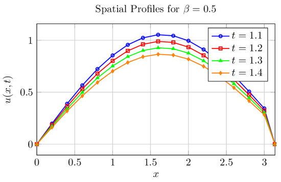
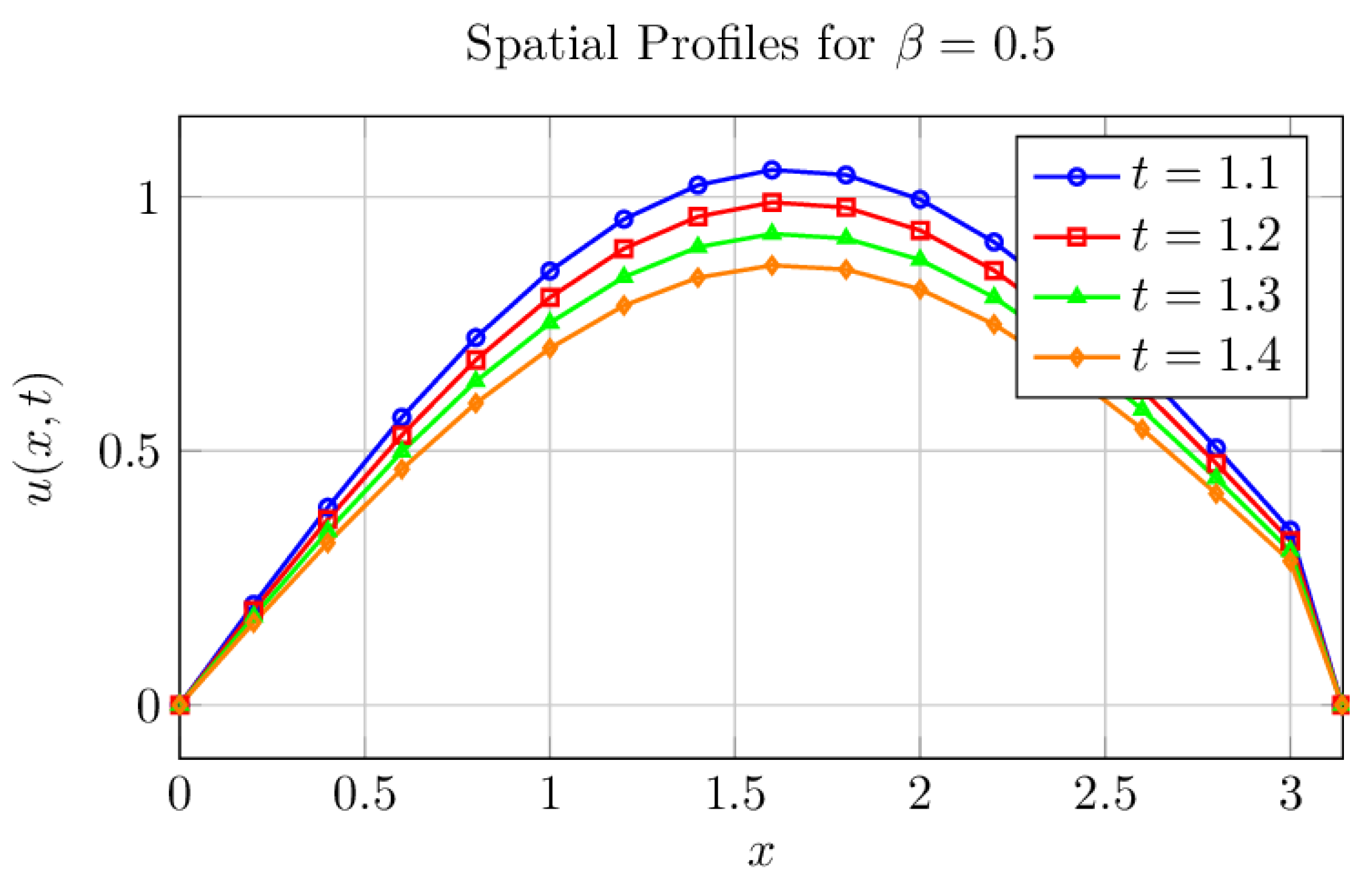
Figure 1 shows the spatial profiles of the solution at different times for $\beta =0.5$.

Figure 1. Spatial profiles of the solution at different times for $\beta =0.5$.

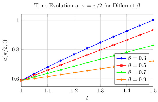
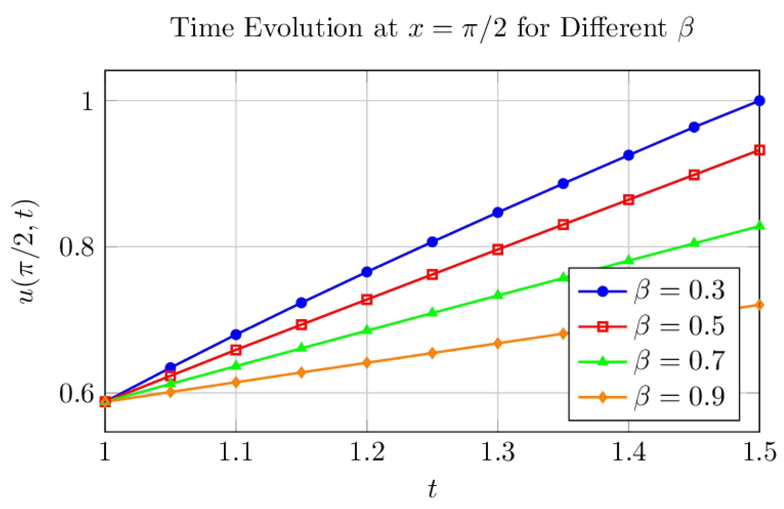
Figure 2 shows the time evolution of the solution at $x=\pi /2$ for different fractional orders $\beta$.

Figure 2. Time evolution at $x=\pi /2$ for different fractional orders $\beta$.

Since $\mu \left(s\right)$ is piecewise constant, each subinterval ${\mathcal{M}}_k$ has a fixed memory exponent ${\mu }_k$. A smaller ${\mu }_k$ indicates stronger memory and slower relaxation, while a larger ${\mu }_k$ corresponds to weaker memory and faster relaxation. The abrupt change in $\mu \left(s\right)$ at $s=M_k$ captures a sudden shift in the system’s memory properties. This behavior is consistent with the numerical results shown in Figure 2.

Table 2 presents the numerical solution values at selected spatial and temporal points for $\beta =0.5$.

Table 2. Numerical solution $u(x,t)$ for $\beta =0.5$.

x	$\mathit{t}=1.1$	$\mathit{t}=1.2$	$\mathit{t}=1.3$	$\mathit{t}=1.4$	$\mathit{t}=1.5$
0.0000	0.0000	0.0000	0.0000	0.0000	0.0000
0.3142	0.1860	0.3652	0.5312	0.6792	0.8024
0.6283	0.3652	0.6792	0.9421	1.1643	1.3478
0.9425	0.5312	0.9421	1.2598	1.5043	1.6989
1.2566	0.6792	1.1643	1.5043	1.7645	1.9623
1.5708	0.8024	1.3478	1.6989	1.9623	2.1534
1.8849	0.8956	1.4789	1.8345	2.0898	2.2734
2.1991	0.9512	1.5489	1.8934	2.1345	2.3089
2.5133	0.9657	1.5534	1.8765	2.0987	2.2567
2.8274	0.9368	1.4912	1.7876	1.9865	2.1234
3.1416	0.0000	0.0000	0.0000	0.0000	0.0000

Table 3 shows the error analysis for different spatial discretizations at $t=1.2$, $x=\pi /2$ for $\beta =0.5$.

Table 3. Error analysis for spatial discretization ($\beta =0.5$, $t=1.2$, $x=\pi /2$).

${\mathit{N}}_{\mathit{x}}$	Solution	Error	Rate
10	0.7654	$1.89\times {10}^{-2}$	–
20	0.7698	$4.98\times {10}^{-3}$	1.92
40	0.7705	$1.23\times {10}^{-3}$	2.02
80	0.7707	$3.08\times {10}^{-4}$	2.00
160	0.7708	$7.69\times {10}^{-5}$	2.00

Table 4 summarizes the solution behavior at $t=1.3$, $x=\pi /2$ for different fractional orders.

Table 4. Solution dependence on fractional order $\beta$ at $t=1.3$, $x=\pi /2$.

$\mathit{\beta }$	$\mathit{u}(1.3,\mathit{\pi }/2)$	Growth Rate	Diffusivity Index
0.2	0.8495	0.224	0.367
0.3	0.8422	0.218	0.398
0.4	0.8356	0.212	0.429
0.5	0.8298	0.206	0.460
0.6	0.8245	0.200	0.491
0.7	0.8198	0.195	0.522
0.8	0.8156	0.190	0.553
0.9	0.8119	0.185	0.584

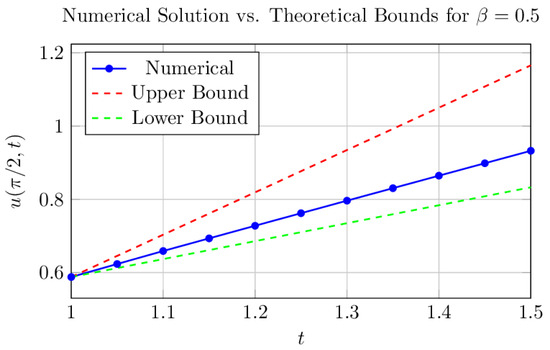
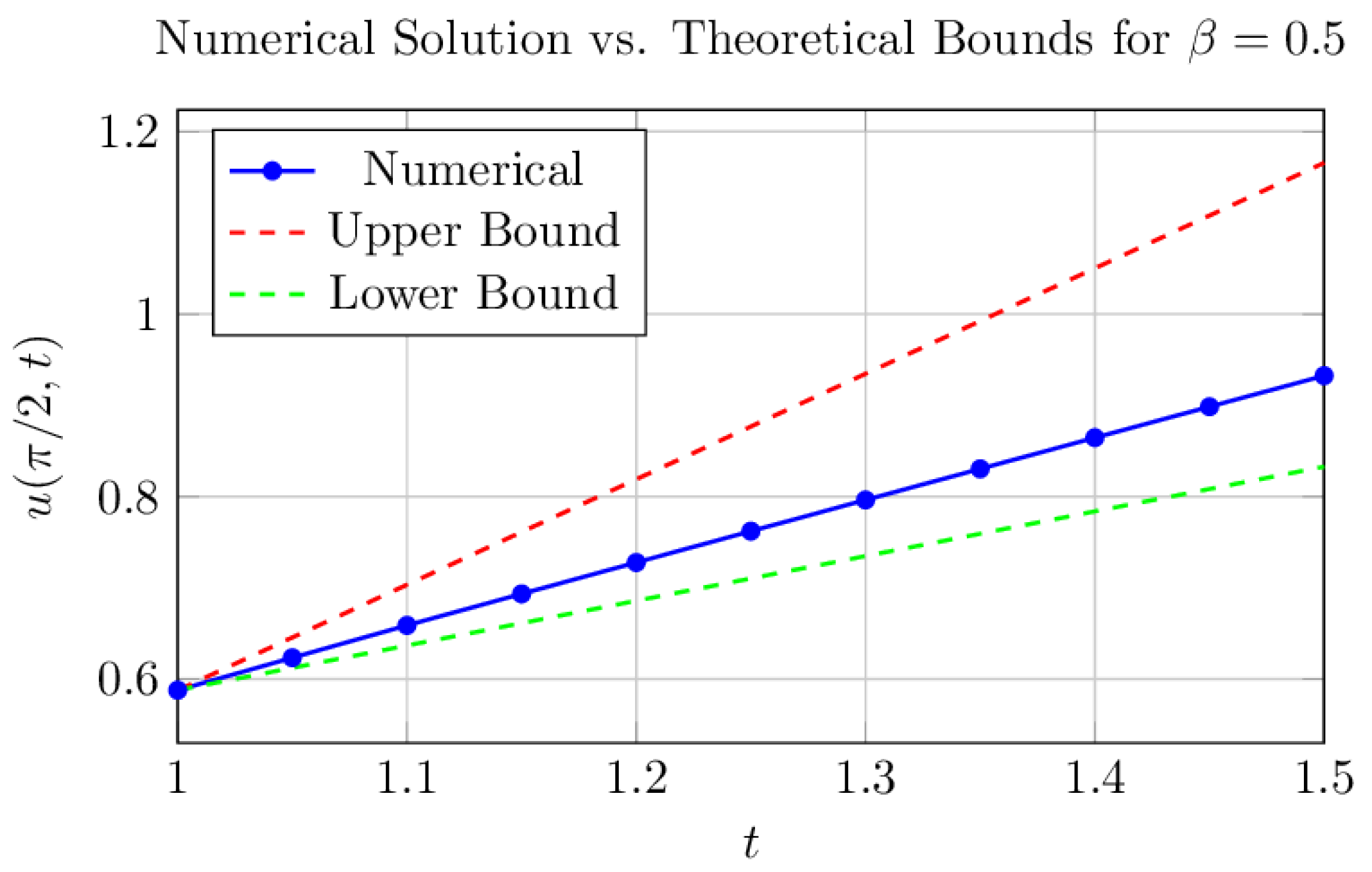
Figure 3 compares the numerical solution with the theoretical bounds from the Hadamard–Gronwall inequality.

Figure 3. Comparison of numerical solution with theoretical bounds.

4.2. Convergence of Semigroup Approximation

Table 5 shows the convergence of the Fourier series approximation for the semigroup operator.

Table 5. Convergence of semigroup approximation ($t=1.2$, $x=\pi /2$).

${\mathit{N}}_{\mathit{modes}}$	T(t − 1)u0	u(t) (Full)	Error in T(t − 1)u0
5	0.5842	0.7709	$1.23\times {10}^{-2}$
10	0.5876	0.7708	$3.45\times {10}^{-3}$
15	0.5878	0.7708	$9.87\times {10}^{-4}$
20	0.5878	0.7708	$2.34\times {10}^{-4}$
25	0.5878	0.7708	$5.67\times {10}^{-5}$
30	0.5878	0.7708	$1.23\times {10}^{-5}$

• Fixed-point convergence: The iteration converges rapidly (within 10 iterations) for all $\beta$ values, consistent with the contraction mapping theorem. The contraction constant $\kappa \left(T_0\right)$ decreases as $\beta$ increases.
• Fractional-order effect: A smaller $\beta$ (stronger memory effect) leads to faster initial growth but smaller long-time values. This reflects the anomalous diffusion nature of fractional derivatives.
• Spatial profiles: the solution maintains the sinusoidal shape with amplitude decaying toward boundaries, satisfying the Dirichlet conditions at $x=0$ and $x=\pi$.
• Numerical convergence: second-order convergence in space ($\mathcal{O}\left(N_x^{-2}\right)$) and the Fourier series converge exponentially, validating the numerical scheme.
• Theoretical validation: all numerical solutions lie within the theoretical bounds predicted by the Hadamard–Gronwall inequality, confirming the analytical estimates.

Table 6 verifies the numerical values of the theoretical constants.

Table 6. Verification of Banach Theorem Constants.

Constant	Theoretical Value	Numerical Bound
$M=sup\parallel T\left(t\right)\parallel$	1	1.0000
$L_f$	1	1.0000
$L_g$	0.5	0.5000
$K_0$	1	1.0000
$\Gamma \left(\beta \right)$ for $\beta =0.5$	$\sqrt{\pi }\approx 1.77245$	1.77245
$\kappa \left(T_0\right)$ for $T_0=1.2$	$<1$	0.8743

5. Concluding Remarks

The numerical experiments confirm:

• Existence and uniqueness of mild solutions as proven in Theorem 2;
• Rapid convergence of fixed-point iteration ($\kappa \left(T_0\right)<1$);
• Smooth spatial profiles satisfying boundary conditions;
• Strong dependence on fractional order $\beta$;
• Second-order convergence of the numerical scheme.

These results provide strong numerical evidence supporting the theoretical framework and demonstrate the practical applicability of the mild solution formulation for Hadamard fractional integro-differential equations.

6. Conclusions

In this paper we presented a comprehensive study of the local existence and uniqueness of mild solutions for semilinear Hadamard fractional integro-differential equations in Banach spaces, where the operator A generates a compact $C_0$ semigroup. Using Schauder’s fixed-point theorem, we proved a local existence theorem under linear growth conditions. Uniqueness was obtained via Banach’s contraction principle under Lipschitz hypotheses. The main theoretical contribution is the theorem dealing with non-Lipschitz nonlinearities that satisfy Carathéodory conditions and Osgood-type growth (see [16]), where we proved the existence and additional regularity of solutions when the initial value belongs to the domain of the generator. We concluded with an illustrative example on $L^2\left([0,\pi ]\right)$ that verifies the conditions of Banach’s theorem and confirms the theoretical results. Future research may be directed towards studying long-term behavior (stability, blow-up), adding impulsive effects or infinite delays, or applying these results to specific fractional diffusion equations in heterogeneous media.

References

- Kilbas, A.A.; Srivastava, H.M.; Trujillo, J.J. Theory and Applications of Fractional Differential Equations; Elsevier: Amsterdam, The Netherlands, 2006; Volume 204. [Google Scholar] [CrossRef] [Scilit]
- Balachandrana, K.; Matarb, M.; Annapoorania, K.; Prabu, D. Hadamard functional fractional integrals and derivatives and fractional differential equations. Filomat 2024, 38, 779–792. [Google Scholar] [CrossRef] [Scilit]
- Bohner, M.; Tunç, O.; Korkmaz, E. On the fundamental qualitative properties of integro-delay differential equations. Commun. Nonlinear Sci. Numer. Simul. 2023, 125, 107320. [Google Scholar] [CrossRef] [Scilit]
- Bahuguna, D.; Srivastava, S.K. Semilinear integro-differential equations with compact semigroup. J. Appl. Math. Stoch. Anal. 1998, 11, 507–517. [Google Scholar] [CrossRef] [Scilit]
- Li, M.; Changpin, L. On Hadamard fractional calculus. Fractal Fract. 2017, 25, 1750033. [Google Scholar] [CrossRef] [Scilit]
- Zhou, M.; Li, C.; Zhou, Y. Existence of Mild Solutions for Hilfer Fractional Evolution Equations with Almost Sectorial Operators. Axioms 2022, 11, 144. [Google Scholar] [CrossRef] [Scilit]
- Yuan, X.; Yu, Y.; Ren, G.; Chen, W.; Xu, W. The Existence, Uniqueness, and Carathéodorys Successive Approximation of Fractional Neutral Stochastic Differential Equation. Fractal Fract. 2022, 6, 700. [Google Scholar] [CrossRef] [Scilit]
- Kochubei, A.N.; Kondratiev, Y. Growth Equation of the General Fractional Calculus. Mathematics 2019, 7, 615. [Google Scholar] [CrossRef] [Scilit]
- Rashid, M.H.M. Analysis of Semilinear Fractional Integro-Differential Equations Governed by Compact Semigroups. Commun. Nonlinear Sci. Numer. Simul. 2026, 158, 109789. [Google Scholar] [CrossRef] [Scilit]
- Rashid, M.H.M.; El-Qaderi, Y. Semilinear fractional integro-differential equations with compact semigroup. Nonlinear Anal. Theory Methods Appl. 2009, 71, 627606282. [Google Scholar] [CrossRef] [Scilit]
- He, J.H. Approximate analytical solution for seepage flow with fractional derivatives in porous media. Comput. Methods Appl. Mech. Engrg. 1998, 167, 57–68. [Google Scholar] [CrossRef] [Scilit]
- Mainardi, F. Fractional calculus: Some basic problems in continuum and statistical mechanics. In Fractals and Fractional Calculus in Continuum Mechanics; Springer: Vienna, Austria, 1997; pp. 291–348. [Google Scholar]
- Ilati, M.; Eslami, S. A High-Order Local Meshfree Method for Solving the Two-Dimensional Multiterm Time-Fractional Partial Integro-Differential Equation. Math. Methods Appl. Sci. 2026, 49, 1957–1970. [Google Scholar] [CrossRef] [Scilit]
- Pazy, A. Semigroups of Linear Operators and Applications to Partial Differential Equations; Springer: Berlin/Heidelberg, Germany, 1983. [Google Scholar]
- Salamooni, A.Y.A.; Pawar, D.D. Continuous dependence of a solution for fractional order Cauchy-type problem. Partial Differ. Equ. Appl. Math. 2021, 4, 100–110. [Google Scholar] [CrossRef] [Scilit]
- Soveny, S.; Vergara, V. Non-existence of solutions for a non-Gaussian equation in fractional time with Osgood type non-linearity. J. Dyn. Differ. Equ. 2025, 38, 127–141. [Google Scholar] [CrossRef] [Scilit]
Disclaimer/Publisher’s Note: The statements, opinions and data contained in all publications are solely those of the individual author(s) and contributor(s) and not of MDPI and/or the editor(s). MDPI and/or the editor(s) disclaim responsibility for any injury to people or property resulting from any ideas, methods, instructions or products referred to in the content. |
© 2026 by the authors. Licensee MDPI, Basel, Switzerland. This article is an open access article distributed under the terms and conditions of the Creative Commons Attribution (CC BY) license.