An Extended Cubic B-Spline Galerkin Finite Element Method for Multi-Term Time-Fractional Differential Equations

Abstract

This study presents an extended cubic B-spline Galerkin scheme for the numerical solution of multi-term time-fractional differential equations. The proposed formulation employs extended cubic B-splines together with the Caputo fractional derivative to model the time-fractional operators. Gauss quadrature is used to accurately evaluate the resulting integral. A stability analysis of the scheme is provided and its accuracy is assessed through $L_2$ and $L_{\infty }$ error norms over different spatial nodes and mesh refinements. The numerical results demonstrate excellent agreement with the exact solutions, as illustrated in the tables and figures. These findings confirm the robustness, efficiency and reliability of the proposed method for solving multi-term time-fractional differential equations.

1. Introduction

Multi-term time-fractional differential equations (MTTF-DEs) arise naturally in modeling of complex physical processes characterized by memory, hereditary effects and anomalous diffusion. Such equations generalize classical diffusion models by incorporating multiple fractional-order temporal derivatives, enabling more accurate descriptions of viscoelastic materials, transport phenomena in porous media, biological systems and non-Newtonian fluids. The general form of MTTF-DEs is given by

$$\begin{array}{cc}\hfill 1& \sum _{i=1}^n{a}_i{\displaystyle \frac{{\partial }^{{\mu }_i}\psi (v,t)}{\partial t^{{\mu }_i}}}={\displaystyle \frac{{\partial }^2\psi (v,t)}{\partial v^2}}+f(v,t),v\in (c,d),t>0,\hfill \\ \hfill \mathrm{initial}\mathrm{condition}:& \hfill \\ \hfill & \psi (v,0)=g\left(v\right),v\in [c,d],\hfill \\ \hfill \mathrm{boundary}\mathrm{conditions}:& \hfill \\ \hfill & \psi (c,t)=h_1\left(t\right),\psi (d,t)=h_2\left(t\right),t>0,\hfill \end{array}$$

(1)

where the coefficients $a_i$ are assumed to be positive constants for $i=1,2,\cdots ,n$ and $g\left(v\right)$, $h_1\left(t\right)$ and $h_2\left(t\right)$ are prescribed functions. The exact solution $\psi (v,t)$ is assumed to be sufficiently smooth, ensuring the existence of required spatial derivatives and the validity of the proposed numerical formulation and stability analysis. Through this work, the fractional orders are assumed to satisfy

$$0<{\mu }_i\le 1,i=1,2,\dots ,m,$$

and the Caputo definition of the fractional derivative is employed. Under appropriate assumptions on the coefficients and the source function, the multi-term time-fractional diffusion equation has a unique solution. Specifically, when $a_i>0$ and ${\mu }_i\in (0,1]$, existence and uniqueness can be proven based on the theory of fractional differential equations of the Caputo type.

Over the past decades, MTTF-DEs have attracted considerable attention and numerous analytical and numerical techniques have been developed, including separation of variables, integral transform methods, spline-based schemes and finite-difference approaches. Kulish and Lage [1] studied the application of the fractional calculus to the anomalous diffusion phenomenon that relates to non-Newtonian fluids. Tarasov [2] used the fractional operators in economy to describe systems with memory and hereditary characteristics. The basic connection between fractional calculus and viscoelasticity has been demonstrated in the work of Bagley and Torvik [3], in which fractional derivatives describe frequency-dependent damping. Arifeen et al. [4] worked on a Galerkin method to solve MTTF-DEs numerically. A correct mathematical formulation of initial boundary value problems for multi-term time-fractional diffusion was provided by Luchko [5]. A numerical method for the solution of MTTF-DEs has been presented using matrix Mittag–Leffler functions by Katsikadelis [6]. Abbas et al. [7] utilized cubic trigonometric B-splines to solve hyperbolic equations numerically. Liu et al. [8] have developed some numerical methods that aim to solve the multi-term time-fractional wave-diffusion equation. Brandibur and Kaslik [9] studied stability features for systems described by multi term time-fractional differential equations. An implicit method for solving multi-term fractional diffusion equation has been formulated by Ravi Kanth and Garg [10]. Ahmad et al. [11] presented a local meshless method to tackle the MTTF-DEs which arise in mathematical physics and biology. Yang and Wu [12] presented a parallel method of natural differences for multi-term time-fractional diffusion equations. Zheng et al. [13] developed a high-order spectral method for solving time fractional-diffusion equation involving multiple terms. Sin et al. [14] have provided analytical solutions for multi-term time-space fractional diffusion equation by using the Caputo-Riesz fractional derivative on an infinite domain. Daftardar-Gejji and Bhalekar [15] examined boundary value formulations that occur in the framework of MTTF-DEs. Li et al. [16] investigated time-fractional diffusion equation with multiple fractional orders, constant positive coefficients and associated initial-boundary value problems. Hussain and Haq [17] proposed weighted meshless spectral method for solving multi-term time-fractional advection-diffusion model for thermo mass transport. Dehghan et al. [18] proposed two high-order numerical methods for multi-term time-fractional diffusion-wave equation. Ren and Sun [19] developed stable and high-efficiency numerical methods for multi-term time-fractional sub-diffusion equation. Edwards et al. initiated works on numerically solving linear multi-term fractional differential equations in the system of equations [20]. In the work by Brandibur and Kaslik [21], a stability analysis was conducted for three fractional derivatives in a MTTF-DE. Bhrawy et al. [22] deduced an effective generalized Laguerre-spectral scheme for solving MTTF-DEs on half-line. A  high-precision numerical scheme of second-order has been designed and proposed by Zeng et al. [23] to solve MTTF-DEs for both smooth and non-smooth solutions. Gazi Karakoc and Geyikli [24] applied a Petrov–Galerkin finite element method for finding a solution for modified regularized long wave equation. Esen and Taşbozan [25] applied a cubic B-spline finite element method to solve the Burgers equation with time fractional derivative. Arifeen et al. [26] conducted a computational investigation of a MTTF-DE using a cubic B-spline finite element method. Jin et al. [27] formed the groundwork of the theoretical analysis for the Galerkin finite element method for a multi-term time-fractional-diffusion equation. Zhang et al. [28] constructed finite difference algorithms for multi-term time-fractional diffusion equations, indicating their efficiency for obtaining accurate and stable numerical solutions. A computational method was presented by Delkhosh and Parand [29] which uses the fractional Lagrange functions for solving multi-term fractional-differential equations, showing better accuracy than other numerical methods. A new numerical technique that employs a combination of cubic B-splines and finite difference method has been introduced by Abu Arqub et al. [30] for solving time-fractional nonlinear diffusion wave equations. Rahman et al. [31] reviewed Caputo fractional derivatives and Riemann–Liouville fractional integrals of various orders and discussed their applications in multi-term differential equations. Abd-Elhameed and Alsuyuti [32] developed a numerical approach using generalized Chebyshev polynomials to efficiently solve multi-term fractional differential equations. Pata et al. [33] investigated multi-term fractional linear equations to model oxygen subdiffusion processes in capillary systems. Santra [34] proposed a higher-order numerical scheme for solving multi-term time-fractional integro-partial differential equations with weakly singular kernels. Mani et al. [35] studied the existence and uniqueness of solutions for multi-term delay Caputo fractional differential equations.

The current spline-based and finite element approaches, such as the classical cubic B-spline Galerkin formulation, possess some shortcomings. These approaches normally make use of static basis sets, limiting their capability for handling solutions that have abrupt gradients or variations. Furthermore, some standard techniques could need mesh refinement in order to improve accuracy, thereby raising the computational expense. Besides, many conventional techniques do not offer an in-built means to regulate the shape attributes of the basis set, which limits their adaptability. In order to resolve the above problems, the current study proposes the application of the extended cubic B-spline Galerkin approach that includes another extended parameter $\lambda$ in its formulation. The inclusion of $\lambda$ increases the adaptability of the basis set without changing the polynomial order of the approach or increasing the number of nodes within the mesh.

The key point of the proposed scheme resides in introducing the extension parameter $\lambda$ to the classical cubic B-spline basis, thus broadening the approximation space while keeping the same order of polynomial degree and meshes involved. As opposed to the traditional cubic B-spline Galerkin scheme, in which the shapes of basis functions remain unchanged, $\lambda$ introduces controllable variation to the basis function shapes in our extended scheme.

In this work, we propose a hybrid numerical framework combining finite differences in time with a Galerkin finite element formulation in space based on extended cubic B-splines. A freely adjustable parameter is introduced within the spline basis, providing enhanced flexibility in controlling approximate behavior. The Caputo definition is introduced within the spline basis, providing enhanced flexibility in controlling approximation behavior. The Caputo definition is employed to approximate temporal fractional derivatives, while numerical integration is performed using a four-point Gaussian quadrature rule for improved precision.

The main contributions of this paper can be summarized as follows:

• An extended cubic B-spline Galerkin formulation is developed for multi-term time-fractional differential equations.
• A flexible extension parameter is incorporated into the spline basis to improve solution accuracy.
• Stability of the fully discrete scheme is analyzed with respect to time step size and fractional orders.
• Convergence is quantitatively assessed using $L_2$ and $L_{\infty }$ error norms.
• Numerical experiments confirm the effectiveness and robustness of the proposed approach.

This paper is further structured as follows: Section 2 presents the detailed derivation of the Galerkin-based numerical scheme using extended cubic B-splines. Section 3 discusses the stability analysis of the proposed scheme. Section 4 presents detailed convergence analysis. Section 5 presents numerical results and a comparison with results from existing numerical schemes in the literature. Section 6 concludes this paper with conclusing remarks.

2. A Galerkin-Based Derivation of the Scheme

In this section, the solution of Equation (1) is obtained by employing extended cubic B-spline basis functions within the framework of the Galerkin finite element method.

2.1. Temporal Discretization

The term involving the fractional derivative in Equation (1) is discretized using the $L_1$ approximation. For a single fractional derivative of order $\mu$ at the time level $t_{n+1}$, the $L_1$ approximation is used to approximate the temporal contribution:

$$\begin{array}{cc}\hfill {\displaystyle \frac{{\partial }^{\mu }}{\partial t^{\mu }}}\psi (v,t_{n+1})& ={\displaystyle \frac{1}{\mathrm{\Gamma }(1-\mu )}}{\int }_0^{t_{n+1}}{\displaystyle \frac{\partial \psi (v,t)}{\partial t}}{(t_{n+1}-t)}^{-\mu }dt\hfill \\ \hfill & ={\displaystyle \frac{1}{\mathrm{\Gamma }(1-\mu )}}\sum _{k=0}^n{\int }_{t_k}^{t_{k+1}}{\displaystyle \frac{\partial \psi (v,t)}{\partial t}}{(t_{n+1}-t)}^{-\mu }dt.\hfill \end{array}$$

(2)

To evaluate the fractional integral in Equation (2), the interval $[0,t_{n+1}]$ is divided into subintervals $[t_k,t_{k+1}]$. On each subinterval, the time derivative ${\displaystyle \frac{\partial \psi (v,t)}{\partial t}}$ is approximated using a first-order finite difference approximation, i.e.,

$${\displaystyle \frac{\partial \psi (v,t)}{\partial t}}\approx {\displaystyle \frac{{\psi }^{k+1}-{\psi }^k}{\Delta t}},t\in [t_k,t_{k+1}].$$

Substituting this approximation into Equation (2) gives

$${\displaystyle \frac{{\partial }^{\mu }\psi (v,t_{n+1})}{\partial t^{\mu }}}\approx {\displaystyle \frac{1}{\mathrm{\Gamma }(1-\mu )}}\sum _{k=0}^n{\displaystyle \frac{{\psi }^{k+1}-{\psi }^k}{\Delta t}}{\int }_{t_k}^{t_{k+1}}{(t_{n+1}-t)}^{-\mu }dt.$$

Now, evaluating the integral term explicitly,

$${\int }_{t_k}^{t_{k+1}}{(t_{n+1}-t)}^{-\mu }dt={\displaystyle \frac{{(t_{n+1}-t_k)}^{1-\mu }-{(t_{n+1}-t_{k+1})}^{1-\mu }}{1-\mu }}.$$

Since $t_k=k\Delta t$, we obtain

$$t_{n+1}-t_k=(n+1-k)\Delta t.$$

Substituting this into the above expression yields a discrete convolution form.

The truncation error arises from the linear approximation of ${\psi }_t$ on each subinterval, which is first-order accurate in time. When combined with the weakly singular kernel ${(t_{n+1}-t)}^{-\mu }$, the global discretization error becomes

$$O(\Delta t^{2-\mu }),$$

which reflects the reduced regularity effect typical in Caputo fractional derivatives. The discretization of the time derivative based on a forward-difference is given by

$$\begin{array}{cc}\hfill {\displaystyle \frac{{\partial }^{\mu }}{\partial t^{\mu }}}\psi (v,t_{n+1})& ={\displaystyle \frac{1}{\mathrm{\Gamma }(1-\mu )}}\sum _{k=0}^n\left[{\displaystyle \frac{{\psi }^{k+1}-{\psi }^k}{\Delta t}}+O(\Delta t)\right]{\int }_{t_k}^{t_{k+1}}{(t_{n+1}-t)}^{-\mu }dt\hfill \\ \hfill & ={\displaystyle \frac{1}{\mathrm{\Gamma }(1-\mu )}}\sum _{k=0}^n\left[{\displaystyle \frac{{\psi }^{k+1}-{\psi }^k}{\Delta t}}\right]{\displaystyle \frac{{(n+1-k)}^{1-\mu }-{(n-k)}^{1-\mu }}{1-\mu }}\Delta t^{1-\mu }+O{(\Delta t)}^{2-\mu }\hfill \\ \hfill & ={\displaystyle \frac{{(\Delta t)}^{-\mu }}{\mathrm{\Gamma }(2-\mu )}}\sum _{k=0}^n\left[{\psi }^{n+1-k}-{\psi }^{n-k}\right]\left[{(k+1)}^{1-\mu }-k^{1-\mu }\right]+O{(\Delta t)}^{2-\mu }.\hfill \end{array}$$

(3)

The obtained expression in Equation (3) can be interpreted as a discrete convolution form, where the fractional derivative is approximated as a weighted sum of past solution increments. This structure is commonly known as the L1 scheme for Caputo fractional derivatives, which is widely used due to its simplicity and effectiveness in handling weakly singular kernels. Recent studies have shown that the L1 approximation achieves accuracy of order $O(\Delta t^{2-\mu })$ under suitable smoothness assumptions of the solution by introducing the following notation:

$$r_{\mu }={\displaystyle \frac{{(\Delta t)}^{-\mu }}{\mathrm{\Gamma }(2-\mu )}},s_{\mu }\left(k\right)={(k+1)}^{1-\mu }-k^{1-\mu }.$$

Equation (3) can be rewritten in the compact form given in Equation (4), which highlights the convolutional structure of the fractional operator.

$${\displaystyle \frac{{\partial }^{\mu }}{\partial t^{\mu }}}\psi (v,t_{n+1})=r_{\mu }\sum _{k=0}^n{s}_{\mu }\left(k\right)\left[{\psi }^{n+1-k}-{\psi }^{n-k}\right]+O{(\Delta t)}^{2-\mu }.$$

(4)

For multi-term fractional operator in Equation (1), the  above approximation is applied to each term:

$$\sum _{i=1}^m{a}_i{\displaystyle \frac{{\partial }^{{\mu }_i}\psi }{\partial t^{{\mu }_i}}}\approx \sum _{i=1}^m{a}_i\left[r_{{\mu }_i}{\psi }^{n+1}-r_{{\mu }_i}{\psi }^n+r_{{\mu }_i}\sum _{k=1}^n{s}_{{\mu }_i}\left(k\right)\left({\psi }^{n+1-k}-{\psi }^{n-k}\right)\right].$$

(5)

where

$$\begin{array}{cc}\hfill r_{{\mu }_i}& ={\displaystyle \frac{{(\Delta t)}^{-{\mu }_i}}{\mathrm{\Gamma }(2-{\mu }_i)}},\hfill \\ \hfill s_{{\mu }_i}\left(k\right)& ={(k+1)}^{1-{\mu }_i}-k^{1-{\mu }_i},i=1,2,\dots ,m.\hfill \end{array}$$

For the multi-term case, each fractional derivative of order ${\mu }_i$ is treated independently using the same L1 discretization framework. The index $i=1,2,\dots ,m$ refers to different fractional orders, while $k=0,1,\dots ,n$ represents the time history levels. To avoid confusion, it is emphasized that the summation over i corresponds to multiple fractional operators, whereas the summation over k represents the temporal convolution within each fractional term.

Remark 1.

As is commonly acknowledged, the solutions to fractional-order differential equations featuring Caputo derivatives tend to show a weakly singular nature at $t=0$. Specifically, the partial derivative of the solution function with respect to time can be approximated by

$${\displaystyle \frac{\partial \psi }{\partial t}}\sim t^{{\mu }_{min}-1},t\to 0.$$

2.2. Extended Cubic B-Spline Special Discretization

In Galerkin approximations, it is possible to employ different functions for the basis and testing functions. In this work, the extended cubic b-spline functions are employed for both basis and testing functions. The region $v\in [c,d]$ is divided into N sub-intervals of equal mesh step

$$h=v_{i+1}-v_i.$$

The Extended cubic B-spline basis function definitions are specified by the following:

$$D_i\left(v\right)={\displaystyle \frac{1}{24h^4}}\left\{\begin{array}{c}{\displaystyle \begin{array}{cc}-4h(\lambda -1){(v-v_i)}^3+3\lambda {(v-v_i)}^4,\hfill & v\in [v_i,v_{i+1}],\hfill \\ (4-\lambda )h^4+12h^3(v-v_{i+1})\hfill & v\in [v_{i+1},v_{i+2}],\hfill \\ +6h^2(2+\lambda ){(v-v_{i+1})}^2\hfill & \hfill \\ -12h{(v-v_{i+1})}^3-3\lambda {(v-v_{i+1})}^4,\hfill & \hfill \\ (16+2\lambda )h^4-12h^2(2+\lambda ){(v-v_{i+2})}^2\hfill & v\in [v_{i+2},v_{i+3}],\hfill \\ +12h(1+\lambda ){(v-v_{i+2})}^3-3\lambda {(v-v_{i+2})}^4,\hfill & \hfill \\ -{(h+v_{i+3}-v)}^3\left[h(\lambda -4)+3\lambda (v-v_{i+3})\right],\hfill & v\in [v_{i+3},v_{i+4}].\hfill \end{array}}\hfill \end{array}\right.$$

(6)

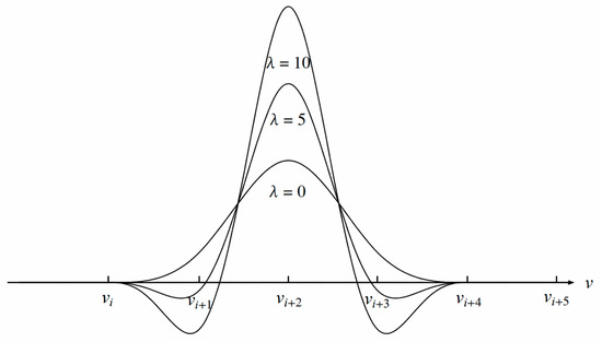
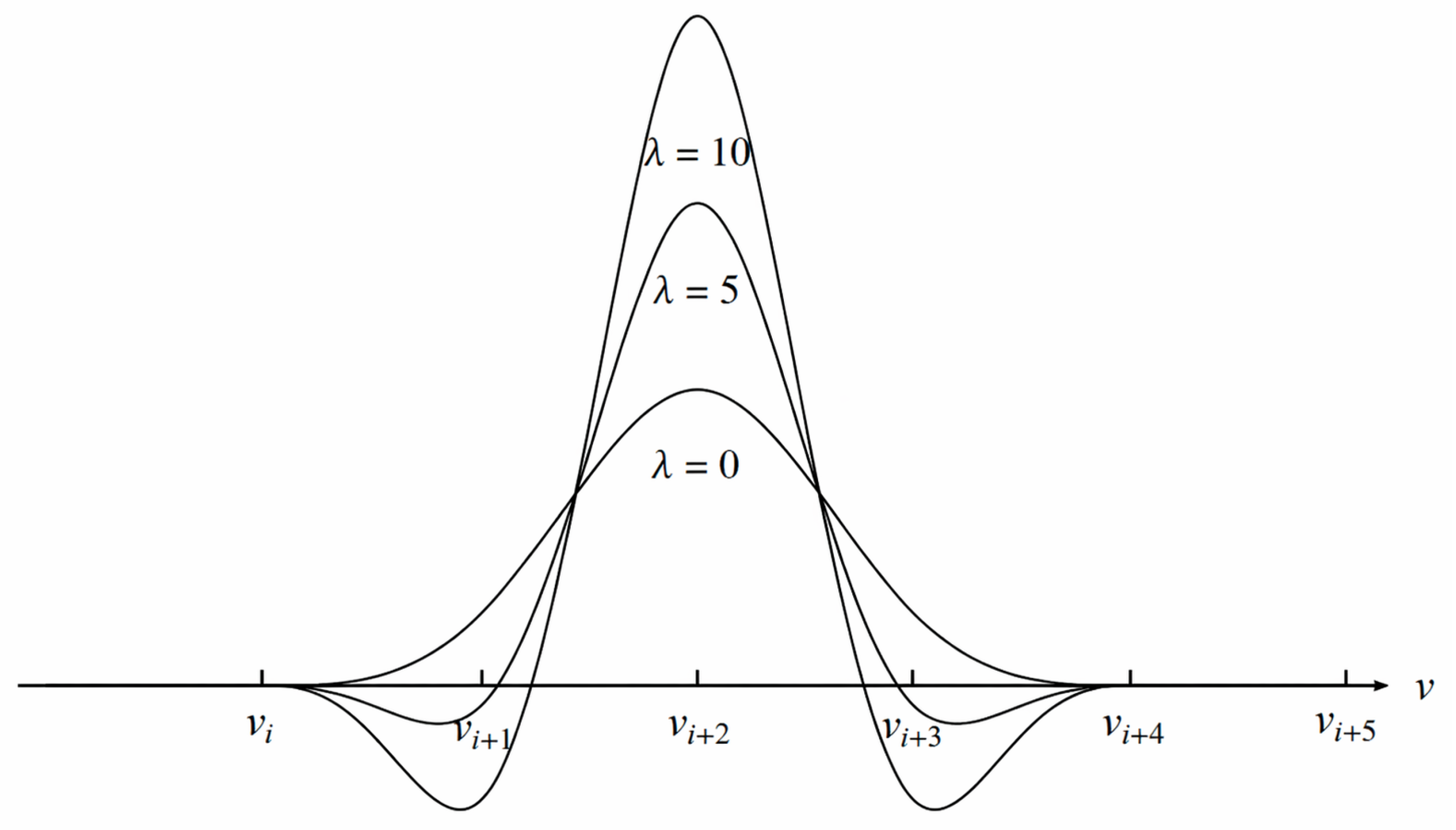
The free parameter $\lambda$ appears in Equation (6), where its presence determines the properties of basis functions. Specifically, it can be used to vary the shape of splines without altering the size of their support or the degree of the polynomial. The basis functions retain their property of being non-zero on four consecutive intervals. For $\lambda \ne 0$, more flexibility is achieved due to extra variations introduced to the basis function shapes, resulting in better approximation performance for steep gradient cases. Figure 1 shows the plots of $D_i\left(v\right)$ for various values of $\lambda$.

Figure 1. Extended cubic B-splines for $\lambda =0,5,10$.

The extended cubic B-spline basis is used to approximate $\psi (v,t)$ as

$$\psi (v,t)\approx \sum _{i=-1}^{N+1}{H}_i\left(t\right)D_i\left(v\right),$$

(7)

where the parameters $H_i$ are unknown and need to be determined. By taking $\delta =v-v_i$, $0\le \delta \le h$ in (6), we obtain

$$\begin{array}{cc}\hfill D_{i-1}& ={\displaystyle \frac{1}{4h^4}}\left({(\delta -h)}^3(h\lambda -4h+3\lambda \delta )\right),\hfill \\ \hfill D_i& ={\displaystyle \frac{1}{4h^4}}\left((16+2\lambda )h^4-12h^2{\delta }^2(2+\lambda )+12h{\delta }^3(1+\lambda )-3\lambda {\delta }^4\right),\hfill \\ \hfill D_{i+1}& ={\displaystyle \frac{1}{4h^4}}\left(h^4(4-\lambda )+12h^3\delta +6h^2{\delta }^2(2+\lambda )-12h{\delta }^3-3\lambda {\delta }^4\right),\hfill \\ \hfill D_{i+2}& ={\displaystyle \frac{1}{4h^4}}\left(4h{\delta }^3(1-\lambda )+3\lambda {\delta }^4\right).\hfill \end{array}$$

(8)

Over the interval $[v_i,v_{i+1}]$, only splines $D_{i-1}$, $D_i$, $D_{i+1}$ and $D_{i+2}$ have non-zero values. Substituting Equation (8) into Equation (7) yields the following:

$$\psi (\delta ,t)\approx \sum _{j=i-1}^{i+2}{H}_j\left(t\right)D_j\left(\delta \right).$$

(9)

The nodal values of $\psi$ and ${\psi }^{\prime }$ are given by

$${\psi }_i={\displaystyle \frac{4-\lambda }{4}}{H}_{i-1}+\left(4+{\displaystyle \frac{\lambda }{2}}\right)H_i+{\displaystyle \frac{4-\lambda }{4}}{H}_{i+1},$$

(10)

$${\psi }_i^{\prime }={\displaystyle \frac{3}{h}}\left(-H_{i-1}+H_{i+1}\right),i=-1,1,0,1,2,\dots ,N+1.$$

(11)

The relationships given in Equations (10) and (11) are obtained by substituting the spline interpolation function defined in Equation (6) and its spatial derivative at the nodal points $v=v_i$. As a result of the compactness of the basis functions associated with extended cubic B-splines, only neighboring basis functions will be active at each node. The substitution will provide the nodal relations in Equation (10) and differentiation will give the derivative relation in Equation (11). The importance of these relations lies in their ability to establish a connection between the nodal solutions and unknown coefficients of the splines in order to formulate the algebraic equations.

2.3. Numerical Formulation by Galerkin-Method

Here, we describe the process of obtaining the numerical solution of Equation (1) using the Galerkin finite element method. An approximate solution $\psi (v,t)$ is sought. Since this approximate solution does not satisfy the governing equation exactly, a residual function $R(v,t)$ is produced. The Galerkin method minimizes the residual in a weighted integral sense over the solution domain $[c,d]$. For this purpose, the governing equation is multiplied by a suitable weight function W and integrated over the domain $[c,d]$.

$${\int }_c^d\left[\sum _{i=1}^n{a}_i{\partial }_t^{{\mu }_i}W\psi +{\displaystyle \frac{\partial W}{\partial v}}{\displaystyle \frac{\partial \psi }{\partial v}}\right]dv-W{\psi }_v{|}_c^d-{\int }_c^{d}Wfdv=0.$$

(12)

By rearranging, we obtain

$${\int }_c^d\left[\sum _{i=1}^n{a}_i{\partial }_t^{{\mu }_i}W\psi +{\displaystyle \frac{\partial W}{\partial v}}{\displaystyle \frac{\partial \psi }{\partial v}}\right]dv-W{\psi }_v{|}_c^d={\int }_c^{d}Wfdv.$$

(13)

To derive the discrete system, we employ the Galerkin method in which the test (weight) functions are chosen from the same space as the basis functions. Specifically, we select the test function as

$$W=D_i\left(v\right),$$

where $D_i\left(v\right)$ denotes the extended cubic B-spline basis functions defined in Equation (6).

The approximate solution $\psi (v,t)$ is expressed in terms of these basis functions as

$$\psi (v,t)\approx \sum _{j=-1}^{N+1}{H}_j\left(t\right)D_j\left(v\right),$$

as given in Equation (7). Substituting this approximation into the weak formulation presented in Equation (12), and taking $W=D_i\left(v\right)$, we obtain

$${\int }_c^d\left(\sum _{k=1}^n{a}_k{\partial }_t^{{\mu }_k}\left(\sum _j{H}_j{D}_j\right)D_i+{\displaystyle \frac{\partial D_i}{\partial v}}{\displaystyle \frac{\partial }{\partial v}}\left(\sum _j{H}_j{D}_j\right)\right)dv-{\left.D_i{\displaystyle \frac{\partial }{\partial v}}\left(\sum _j{H}_j{D}_j\right)\right|}_c^d={\int }_c^d{D}_{i}fdv.$$

Rearranging the terms and interchanging summation and integration, we obtain integrals involving products of basis functions and their derivatives. Due to the compact support of the extended cubic B-splines, each basis function $D_i\left(v\right)$ overlaps only with the neighboring functions $D_{i-1}\left(v\right)$, $D_i\left(v\right)$, $D_{i+1}\left(v\right)$ and $D_{i+2}\left(v\right)$. Therefore, the summation reduces locally to $j=i-1,i,i+1,i+2$, leading directly to the element-wise formulation given in Equation (14).

$$\sum _{j=i-1}^{i+2}{\int }_{v_i}^{v_{i+1}}\left(D_i{D}_j\left[\sum _{i=1}^n{a}_i{\partial }_t^{{\mu }_i}\right]+D_i^{\prime }{D}_j^{\prime }{H}_j\right)dx-D_i{D}_j^{\prime }{H}_j{|}_{v_i}^{v_{i+1}}={\int }_{v_i}^{v_{i+1}}{D}_{i}fdv.$$

(14)

substituting Equation (8) in Equation (14) gives

$$\sum _{j=i-1}^{i+2}\left\{\left(\underset{0}{\overset{h}{\int }}{D}_i{D}_{j}d\delta \right)\left[\sum _{i=1}^n{c}_i{\displaystyle \frac{{\partial }^{{\mu }_i}{H}_j}{\partial t^{{\mu }_i}}}\right]+\left(\underset{0}{\overset{h}{\int }}{D}_i^{\prime }{D}_j^{\prime }d\delta \right)H_j-D_i{D}_j^{\prime }{H}_j{|}_0^h\right\}=\underset{0}{\overset{h}{\int }}{D}_{i}f(\delta +v_i,t)d\delta .$$

(15)

Each of the matrices occurring in Equation (15) can be understood physically and numerically. The matrix that comes from the time derivative term is the mass matrix, resulting from the inner product of the basis functions. The matrix that comes from the spatial derivatives term is known as the stiffness matrix, accounting for the diffusion terms. Furthermore, the contribution from the boundary condition results in the boundary vector/matrix. Let

$$C_1^e=\underset{0}{\overset{h}{\int }}{D}_i{D}_{j}d\delta ,i,j=i-1,i,i+1,i+2$$

$$C_2^e=\underset{0}{\overset{h}{\int }}{D}_i^{\prime }{D}_j^{\prime }d\delta ,i,j=i-1,i,i+1,i+2$$

$$C_3^e=D_i{D}_j^{\prime }{|}_0^h,i,j=i-1,i,i+1,i+2$$

$$F_e={\int }_0^h{D}_{i}f(\delta +v_i,t)d\delta i=i-1,i,i+1,i+2.$$

A matrix form of Equation (15) is given by

$$\sum _{i=1}^n{a}_i{C}_1^e{\displaystyle \frac{{\partial }^{{\mu }_i}{H}^e}{\partial t^{{\delta }_i}}}+\left(C_2^e-C_3^e\right)H^e=F_e.$$

(16)

While the exact forms of $C_1^e$, $C_2^e$ and $C_3^e$ are quite long, they are listed below for sake of completeness. It should be emphasized that the matrices have good structural characteristics.

$$C_1^e=\left(\begin{array}{cccc}{\int }_0^h{C}_{i-1}{C}_{i-1}d\delta & {\int }_0^h{C}_{i-1}{C}_{i}d\delta & {\int }_0^h{C}_{i-1}{C}_{i+1}d\delta & {\int }_0^h{C}_{i-1}{C}_{i+2}d\delta \\ {\int }_0^h{C}_i{C}_{i-1}d\delta & {\int }_0^h{C}_i{C}_{i}d\delta & {\int }_0^h{C}_i{C}_{i+1}d\delta & {\int }_0^h{C}_i{C}_{i+2}d\delta \\ {\int }_0^h{C}_{i+1}{C}_{i-1}d\delta & {\int }_0^h{C}_{i+1}{C}_{i}d\delta & {\int }_0^h{C}_{i+1}{C}_{i+1}d\delta & {\int }_0^h{C}_{i+1}{C}_{i+2}d\delta \\ {\int }_0^h{C}_{i+2}{C}_{i-1}d\delta & {\int }_0^h{C}_{i+2}{C}_{i}d\delta & {\int }_0^h{C}_{i+2}{C}_{i+1}d\delta & {\int }_0^h{C}_{i+2}{C}_{i+2}d\delta \end{array}\right),$$

$$C_1^e=h\left(\begin{array}{cccc}{\displaystyle \frac{(8+11\lambda +{\lambda }^2)}{56}}& {\displaystyle \frac{(258-147\lambda -37{\lambda }^2)}{1120}}& {\displaystyle \frac{(48-129\lambda +14{\lambda }^2)}{560}}& {\displaystyle \frac{(8-10\lambda +3{\lambda }^2)}{1120}}\\ {\displaystyle \frac{(258-147\lambda -37{\lambda }^2)}{1120}}& {\displaystyle \frac{(4752+585\lambda +44{\lambda }^2)}{560}}& {\displaystyle \frac{(3732+27\lambda -65{\lambda }^2)}{1120}}& {\displaystyle \frac{(48-129\lambda +14{\lambda }^2)}{560}}\\ {\displaystyle \frac{(48-129\lambda +14{\lambda }^2)}{560}}& {\displaystyle \frac{(3732+27\lambda -65{\lambda }^2)}{1120}}& {\displaystyle \frac{(4752+585\lambda +44{\lambda }^2)}{560}}& {\displaystyle \frac{(258-147\lambda -37{\lambda }^2)}{1120}}\\ {\displaystyle \frac{(8-10\lambda +3{\lambda }^2)}{1120}}& {\displaystyle \frac{(48-129\lambda +14{\lambda }^2)}{560}}& {\displaystyle \frac{(258-147\lambda -37{\lambda }^2)}{1120}}& {\displaystyle \frac{(8+11\lambda +{\lambda }^2)}{56}}\end{array}\right),$$

$$C_2^e=\left(\begin{array}{cccc}{\int }_0^h{C}_{i-1}^{\prime }{C}_{i-1}^{\prime }d\delta & {\int }_0^h{C}_{i-1}^{\prime }{C}_i^{\prime }d\delta & {\int }_0^h{C}_{i-1}^{\prime }{C}_{i+1}^{\prime }d\delta & {\int }_0^h{C}_{i-1}^{\prime }{C}_{i+2}^{\prime }d\delta \\ {\int }_0^h{C}_i^{\prime }{C}_{i-1}^{\prime }d\delta & {\int }_0^h{C}_i^{\prime }{C}_i^{\prime }d\delta & {\int }_0^h{C}_i^{\prime }{C}_{i+1}^{\prime }d\delta & {\int }_0^h{C}_i^{\prime }{C}_{i+2}^{\prime }d\delta \\ {\int }_0^h{C}_{i+1}^{\prime }{C}_{i-1}^{\prime }d\delta & {\int }_0^h{C}_{i+1}^{\prime }{C}_i^{\prime }d\delta & {\int }_0^h{C}_{i+1}^{\prime }{C}_{i+1}^{\prime }d\delta & {\int }_0^h{C}_{i+1}^{\prime }{C}_{i+2}^{\prime }d\delta \\ {\int }_0^h{C}_{i+2}^{\prime }{C}_{i-1}^{\prime }d\delta & {\int }_0^h{C}_{i+2}^{\prime }{C}_i^{\prime }d\delta & {\int }_0^h{C}_{i+2}^{\prime }{C}_{i+1}^{\prime }d\delta & {\int }_0^h{C}_{i+2}^{\prime }{C}_{i+2}^{\prime }d\delta \end{array}\right),$$

$$C_2^e={\displaystyle \frac{1}{140h}}·\left(\begin{array}{cccc}4(63-21\lambda +3{\lambda }^2)& 294-33{\lambda }^2& -504+84\lambda +60{\lambda }^2& -42+42\lambda -9{\lambda }^2\\ 294-33{\lambda }^2& 1428+672\lambda +96{\lambda }^2& -1218-714\lambda -93{\lambda }^2& -504+84\lambda +60{\lambda }^2\\ -504+84\lambda +60{\lambda }^2& -1218-714\lambda -93{\lambda }^2& 1428+672\lambda +96{\lambda }^2& 294-33{\lambda }^2\\ -42+42\lambda -9{\lambda }^2& -504+84\lambda +60{\lambda }^2& 294-33{\lambda }^2& 4(63-21\lambda +3{\lambda }^2)\end{array}\right),$$

$$C_3^e=\left(\begin{array}{cccc}{C}_{i-1}{C}_{i-1}^{\prime }{|}_0^h& C_{i-1}{C}_i^{\prime }{|}_0^h& C_{i-1}{C}_{i+1}^{\prime }{|}_0^h& C_{i-1}{C}_{i+2}^{\prime }{|}_0^h\\ C_i{C}_{i-1}^{\prime }{|}_0^h& C_i{C}_i^{\prime }{|}_0^h& C_i{C}_{i+1}^{\prime }{|}_0^h& C_i{C}_{i+2}^{\prime }{|}_0^h\\ C_{i+1}{C}_{i-1}^{\prime }{|}_0^h& C_{i+1}{C}_i^{\prime }{|}_0^h& C_{i+1}{C}_{i+1}^{\prime }{|}_0^h& C_{i+1}{C}_{i+2}^{\prime }{|}_0^h\\ C_{i+2}{C}_{i-1}^{\prime }{|}_0^h& C_{i+2}{C}_i^{\prime }{|}_0^h& C_{i+2}{C}_{i+1}^{\prime }{|}_0^h& C_{i+2}{C}_{i+2}^{\prime }{|}_0^h\end{array}\right),$$

$$C_3^e={\displaystyle \frac{3}{4h}}\left(\begin{array}{cccc}-(\lambda -4)& 0& (\lambda -4)& 0\\ 2(8+\lambda )& (\lambda -4)& -2(8+\lambda )& -(\lambda -4)\\ -(\lambda -4)& -2(8+\lambda )& (\lambda -4)& 2(8+\lambda )\\ 0& (\lambda -4)& 0& -(\lambda -4)\end{array}\right),$$

$$F_e=\left(\begin{array}{c}{\int }_0^h{D}_{i-1}d\delta \\ {\int }_0^h{D}_{i}fd\delta \\ {\int }_0^h{D}_{i+1}fd\delta \\ {\int }_0^h{D}_{i+2}fd\delta \end{array}\right).$$

The sparsity and bandedness of the overall system matrices can be attributed to the fact that the basis functions have a finite support region due to which only a few adjacent basis functions will interact with any given basis function. In addition to these attributes, $C_1^e$ and $C_2^e$ are symmetric matrices, while $C_3^e$ stems from the boundary terms. The vector $F_e$ is approximated using the four-point Gauss quadrature rule.

2.4. Global System Assembly

The local element formulations interact through global assembly to form the following system:

$$\sum _{i=1}^n{a}_i{D}_1{\displaystyle \frac{{\partial }^{{\mu }_i}H}{\partial t^{{\mu }_i}}}+(D_2-D_3)H=F$$

(17)

where G is the global vector of unknown coefficients, $H_1$ is the global mass matrix, $H_2$ and $H_3$ are the global stiffness-related matrices and F is the global load vector. The assembly of the finite elements leads to the formation of the global matrices, which have a banded structure. Matrices $D_1$, $D_2$ and $D_3$ are used to denote the contributions of the global system, which are calculated using the elemental matrices assembly procedure. $D_1$ denotes the mass matrix that comes with the time derivative, $D_2$ is the stiffness matrix resulting from the spatial derivative and $D_3$ represents the fractional operator contribution. The resulting global matrices $D_1$, $D_2$ and $D_3$ takes the form

$$D_1={\displaystyle \frac{h}{140}}\left(1,120+60\lambda ,1191-120\lambda ,2416+240\lambda ,1191-120\lambda ,120+60\lambda ,1\right),$$

$$D_2={\displaystyle \frac{1}{10h}}\left(-3,-72+36\lambda ,-45+18\lambda ,240,-45+18\lambda ,-72+36\lambda ,-3\right),$$

$$D_3={\displaystyle \frac{3}{h}}\left(0,0,0,0,0,0,0\right).$$

2.5. Full Disretization

Substituting the temporal dicretization Equation (5) into Equation (17) and using the weighted average $(\theta -method)$ for the spatial terms, gives

$$D_4{H}^{n+1}=D_5{H}^n+D_6,$$

(18)

where

$$D_4=\left(\sum _{i=1}^m{a}_i{r}_{{\mu }_i}{D}_1+\theta D_2-\theta D_3\right),$$

(19)

$$D_5=\left(\sum _{i=1}^m{a}_i{r}_{{\mu }_i}{D}_1-(1-\theta )D_2+(1-\theta )D_3\right),$$

(20)

$$D_6=\theta F^{n+1}+(1-\theta )F^n-\sum _{i=1}^m{a}_i{r}_{{\mu }_i}\sum _{k=1}^n{s}_{{\mu }_i}\left(k\right)\left[H^{n+1-k}-H^{n-k}\right]D_1.$$

(21)

The operator $D_6$ includes the history effect characteristic of Caputo-type fractional derivatives. This operator is computed at each step by means of a discrete convolution that utilizes the solution vectors $H^{n-k}$ and $H^{n+1-k}$ from the previous steps. In actual computation, the terms

$$s_{{\mu }_i}\left(k\right)={(k+1)}^{1-{\mu }_i}-k^{1-{\mu }_i}$$

that solely depend on ${\mu }_i$ and k, are calculated prior to any iterations and stored for use in the computations. As the operator $D_1$ does not change after assembly, the history operator is easily computed using the solution vectors obtained during previous computations without having to reconstruct the matrix again.

2.6. Initial Matrix Implementation

Let ${\left\{L_m\left(v\right)\right\}}_{m=-1}^{N+1}$ represent the basis formed by extended cubic B-splines with extension parameter $\lambda$ and equal step size h. The initial value ${\mathbf{H}}^0$ is determined by Equation (9). The unknown coefficients at each time level are then obtained from Equation (18). To calculate ${\mathbf{H}}^0$ Equation (9) at $t=0$ becomes

$$\psi (v,0)=\sum _{m=-1}^{N+1}{H}_m^0{D}_m\left(v\right),$$

(22)

where $\psi$ and ${\psi }^{\prime }$ are denoted as

$$\begin{array}{cc}\hfill \psi (v_i,0)& =p\left(v_i\right),i=0,1,\dots ,N-1,\hfill \\ \hfill {\psi }^{\prime }(v_0,0)& =p^{\prime }\left(v_0\right),\hfill \\ \hfill {\psi }^{\prime }(v_N,0)& =p^{\prime }\left(v_N\right).\hfill \end{array}$$

This yields an $(N+3)\times (N+3)$ system of equations:

$${\mathbf{S}}_4{\mathbf{H}}^0={\mathbf{S}}_5$$

(23)

$$\underset{(N+3)\times (N+3)}{\underbrace{\left[\begin{array}{cccccc}1& -2& 1& 0& \dots & 0\\ 4-\lambda & 16+2\lambda & 4-\lambda & 0& \dots & 0\\ 0& 4-\lambda & 16+2\lambda & 4-\lambda & \dots & 0\\ ⋮& \ddots & \ddots & \ddots & \ddots & ⋮\\ 0& \dots & 4-\lambda & 16+2\lambda & 4-\lambda & 0\\ 0& \dots & 0& 4-\lambda & 16+2\lambda & 4-\lambda \\ 0& \dots & -(1-\lambda )& 0& (1-\lambda )& 0\\ 0& \dots & 0& 1& -2& 1\end{array}\right]}}\underset{N+3}{\underbrace{\left[\begin{array}{c}{H}_{-1}\\ H_0\\ ⋮\\ H_{N+1}\end{array}\right]}}=\underset{N+3}{\underbrace{\left[\begin{array}{c}p\left(v_{-1}\right)\\ p\left(v_0\right)\\ p\left(v_1\right)\\ ⋮\\ p\left(v_{N-2}\right)\\ p\left(v_{N-1}\right)\\ p^{\prime }\left(v_N\right)\\ p\left(v_{N+1}\right)\end{array}\right]}}$$

Equation (23) emerges after imposing the initial and boundary conditions to the expanded extended cubic B-spline in Equation (22). This results in a system of linear equations of dimension $(N+3)\times (N+3)$, where the coefficients of the equation $H^0$ are unknown. The extra equations in the linear system can be generated from the derivatives of the boundary conditions, providing closure in the system. The coefficient matrix derived from the linear system becomes a band matrix because of the finite nature of the basis function. Given that the extended cubic B-spline basis functions are linearly independent and the boundary conditions are properly set, the system matrix remains non-singular. The implementation of the presented scheme is summarized in Algorithm 1.

Algorithm 1 Numerical solution procedure.
Step	Description
1	Discretize the spatial domain $[c,d]$ into N elements with step size h and the time domain with step size $\Delta t$.
2	Construct extended cubic B-spline basis functions $D_i\left(v\right)$ and compute element matrices $C_1^e$, $C_2^e$ and $C_3^e$.
3	Assemble global matrices $D_1$, $D_2$ and $D_3$.
4	Compute initial coefficient vector $H^0$ from Equation (23) using initial and boundary conditions.
5	For each time level $n=0,1,2,\dots$:
	(a) Compute right-hand side vector using Equation (21).
	(b) Form matrices $D_4$ and $D_5$ using Equations (19) and (20).
	(c) Solve $D_4{H}^{n+1}=D_5{H}^n+D_6$.
6	Repeat Step 5 until final time level is reached.
7	Obtain approximate solution $\psi (v,t)$ using Equation (9).

3. Stability Analysis

We now analyze the stability of proposed procedure using the matrix method. To define the error at time level n, we introduce

$${\mathbf{E}}^n={\overline{\mathbf{\psi }}}^n-{\mathbf{\psi }}^n,$$

(24)

where $\overline{\mathbf{\psi }}$ denotes the exact solution and $\mathbf{\psi }$ represents the approximate solution. From Equation (18), we have

$${\mathbf{D}}_{\mathbf{4}}{\mathbf{H}}^{n+1}={\mathbf{D}}_{\mathbf{5}}{\mathbf{H}}^n+{\mathbf{D}}_{\mathbf{6}}.$$

(25)

Assume that ${\mathbf{D}}_{\mathbf{4}}$ is nonsingular, so that ${\mathbf{D}}_{\mathbf{4}}^{-1}$ exists. Then Equation (25) can be written as

$${\mathbf{H}}^{n+1}={\mathbf{D}}_{\mathbf{4}}^{-1}{\mathbf{D}}_{\mathbf{5}}{\mathbf{H}}^n+{\mathbf{D}}_{\mathbf{4}}^{-1}{\mathbf{D}}_{\mathbf{6}}.$$

(26)

Here, ${\mathbf{D}}_{\mathbf{4}}^{-1}{\mathbf{D}}_{\mathbf{5}}$ is the amplification matrix. If $\psi$ denote the approximate solution vector, then

$${\mathit{\psi }}^{n+1}=\mathbf{A}{\mathbf{D}}^{n+1},{\mathit{\psi }}^n=\mathbf{A}{\mathbf{D}}^n.$$

(27)

Using Equations (24), (26) and (27), we obtain

$${\mathbf{E}}^{n+1}=\mathbf{U}{\mathbf{E}}^n,$$

(28)

where the amplification matrix $\mathbf{U}$ is defined by

$$\mathbf{U}=\mathbf{A}{\mathbf{D}}_{\mathbf{4}}^{-1}{\mathbf{D}}_{\mathbf{5}}{\mathbf{D}}^{-1}.$$

As the parameter $\lambda$ occurs explicitly in the element matrices $C_1^e$, $C_2^e$ and $C_3^e$, the matrices $D_1$, $D_2$ and $D_3$ will depend on the parameter $\lambda$ too. Hence, the amplification matrix can be expressed as

$$\mathbf{U}\left(\lambda \right)={\mathbf{D}}_{\mathbf{4}}{\left(\lambda \right)}^{-1}{\mathbf{D}}_{\mathbf{5}}\left(\lambda \right).$$

For the numerical solution to be stable, the error must remain bounded at all time levels. Therefore, for fixed value of $\lambda$ the following condition is required:

$$\parallel \mathbf{U}\left(\lambda \right)\parallel \le 1.$$

(29)

If $\mathbf{U}\left(\lambda \right)$ is symmetric, then its norm is equal to its spectral radius, that is

$$\parallel \mathbf{U}\left(\lambda \right)\parallel =\xi \left(\mathbf{U}\right(\lambda \left)\right),$$

(30)

where $\xi \left(\mathbf{U}\right(\lambda \left)\right)$ denotes the spectral radius of the matrix $\mathbf{U}\left(\lambda \right)$. In general, the inequality

$$\xi \left(\mathbf{U}\right(\lambda \left)\right)\le \parallel \mathbf{U}\left(\lambda \right)\parallel$$

(31)

always holds. The stability of the proposed scheme is ensured provided that the spectral radius of the amplification matrix $\mathbf{U}$ satisfies

$$\xi \left(\mathbf{U}\right(\lambda \left)\right)\le 1,$$

which guarantees that the error remains bounded at all time levels. This condition follows from the matrix form of the scheme and is standard in the analysis of time-stepping methods.

The stability criterion is obtained from the matrix representation of the fully discrete scheme, where the growth of the error is controlled by the amplification matrix $\mathbf{U}\left(\lambda \right)$. The stability requirement that the spectral radius satisfy

$$\xi \left(\mathbf{U}\right(\lambda \left)\right)\le 1$$

ensures that the error cannot increase without bound at any time level. This condition is also well-aligned with the classical stability analysis of linear time-marching methods. Here, the appearance of the relevant matrices is due to the application of the Galerkin method based on the extended cubic B-spline basis functions, which have finite support. This implies that the resulting system matrices will be sparse and banded. Additionally, the application of the L1 method for approximating the Caputo derivative gives rise to the inclusion of a weighted history term, which is known to be stable under small step-size assumptions. Consequently, the proposed combination of the Galerkin method and the L1 approach will yield a stable numerical scheme under the specified condition.

4. Convergence Analysis

In this section, a comprehensive convergence analysis of the proposed numerical scheme is presented.

Theorem 1.

Suppose that the exact solution of the multi-term time-fractional differential Equation (1) is sufficiently smooth and the fully discrete extended cubic B-spline Galerkin method is consistent. Furthermore, assume that the L1 approximation is used for each Caputo derivative of order ${\mu }_i\in (0,1]$, while the spatial Galerkin discretization is of second-order. Provided that the fully discrete method is stable in the sense that the error is uniformly bounded at all discrete time levels, the numerical solution converges to the exact solution. Furthermore, the global error between the exact and numerical solutions obeys

$$\parallel \psi (·,t_n)-{\psi }_h^n\parallel \le C\left(\Delta t^{2-{\mu }_{max}}+h^2\right),$$

where ${\mu }_{max}=max\{{\mu }_1,{\mu }_2,\dots ,{\mu }_m\}$.

Proof. 

The proof is based on the consistency and stability properties of the proposed fully discrete scheme.

In terms of the temporal discretization, the error term in approximating the Caputo fractional derivative of order ${\mu }_i\in (0,1]$ by L1 scheme is of the order

$$\mathcal{O}(\Delta t^{2-{\mu }_i}).$$

Consequently, the leading error term associated with multi-term fractional derivative operator will be determined by the largest order of differentiation, which is

$$\mathcal{O}(\Delta t^{2-{\mu }_{max}}),{\mu }_{max}=max\{{\mu }_1,{\mu }_2,\dots ,{\mu }_m\}.$$

With regard to the spatial discretization, provided that the exact solution is sufficiently smooth, the extended cubic B-spline Galerkin approximation gives second-order accuracy, or equivalently,

$$\mathcal{O}\left(h^2\right).$$

Therefore, the fully discrete scheme is consistent with the order

$$\mathcal{O}(\Delta t^{2-{\mu }_{max}}+h^2).$$

Let

$$E^n={\overline{H}}^n-H^n$$

be the error vector at the time level $t_n$, where ${\overline{H}}^n$ and $H^n$ stand for the exact and numerical coefficient vectors, respectively. In terms of the matrix form of the scheme, the error fulfills a discrete equation of the kind

$$E^{n+1}=U{E}^n+{\tau }^n,$$

where U is the amplification matrix and ${\tau }^n$ represents the local truncation error.

In the case where the scheme is stable, the discrete solution operator becomes uniformly bounded, and, hence, we have

$$\parallel E^n\parallel \le C\left(\parallel E^0\parallel +\underset{0\le j\le n-1}{max}\parallel {\tau }^j\parallel \right).$$

Because the initial conditions are prescribed consistently, $\parallel E^0\parallel =0$, and since

$$\parallel {\tau }^j\parallel \le C\left(\Delta t^{2-{\mu }_{max}}+h^2\right),$$

it follows that

$$\parallel E^n\parallel \le C\left(\Delta t^{2-{\mu }_{max}}+h^2\right).$$

Therefore, the numerical solution converges to the exact solution with order

$$\mathcal{O}(\Delta t^{2-{\mu }_{max}}+h^2).$$

This completes the proof. □

5. Numerical Results and Discussions

This section presents the application of the proposed scheme to the solution of MTTF-DEs. The efficiency and accuracy of the presented method are rigorously tested through comparison with the exact solution and with existing approaches reported in the literature. The numerical accuracy is accessed by means of the $L_{\infty }$ and $L_2$ norms, which provide a quantitative measure of the approximation error:

$$L_{\infty }=\underset{q}{max}\left|{\psi }_q-{\tilde{\psi }}_q\right|,$$

(32)

$$L_2=\sqrt{h\sum _{q=1}^N{\left|{\psi }_q-{\tilde{\psi }}_q\right|}^2}.$$

(33)

Here h denotes the spatial grid size, N is the total number of grid points, ${\psi }_q$ represents the exact solution, and ${\tilde{\psi }}_q$ denotes the numerical solution at the grid point q. Moreover, to compute the convergence of the numerical method, we use the relation

$$\mathrm{Rate}\mathrm{of}\mathrm{Convergence}(\mathrm{R}.\mathrm{C}.)={log}_2\left({\displaystyle \frac{L_{\infty }(h,2\Delta t)}{L_{\infty }(h,\Delta t)}}\right).$$

(34)

Remark 2.

It should be emphasized that using a uniform time grid may not be sufficient to account for the weak singularity at $t=0$ present in Caputo-type fractional problems. In this case, it is possible to use non-uniform time grids to enhance the convergence of the numerical approximation. One of the most common approaches is to apply the following graded time grid:

$$t_n={\left({\displaystyle \frac{n}{N}}\right)}^{r}T,r>1.$$

The advantages of using a non-uniform time grid have been proven for fractional problems, where the presence of a weak singularity at $t=0$ leads to a loss of optimal convergence rate. Nevertheless, in this paper, we consider the problem on a uniform grid for simplicity, leaving the extension of our approach to the non-uniform case as a subject of further research.

Remark 3.

It is worth noting that the error norms reported at the final time level inherently reflect the cumulative effect of the temporal discretization, since the numerical solution at the final time depends on all previous time steps. Therefore, these results provide an effective measure of the global accuracy of the scheme for time-fractional problems.

Remark 4.

Although the test problems considered in this study are smooth, it is well known that solutions of time-fractional equations generally exhibit weak singularity near $t=0$. The consistent convergence behavior observed in the numerical results indicates that the proposed method remains robust under such limited regularity.

The proposed scheme is now applied to determine the numerical solution of selected MTTF-DE’s.

Example 1.

The two-term time-fractional differential equation is given by

$$\sum _{i=1}^2{a}_i{\displaystyle \frac{{\partial }^{{\mu }_i}\psi (v,t)}{\partial t^{{\mu }_i}}}-{\displaystyle \frac{{\partial }^2\psi (v,t)}{\partial v^2}}=\left(2t-t^2+{\displaystyle \frac{2t^{2-{\mu }_2}}{\mathrm{\Gamma }(3-{\mu }_2)}}\right)e^v,$$

(35)

with the initial condition

$$\psi (v,0)=0,v\in [0,1]$$

(36)

and boundary conditions

$$\psi (0,t)=t^2,\psi (v,t)=e·t^2,$$

(37)

while the exact solution is

$$\psi (v,t)=e^v{t}^2.$$

(38)

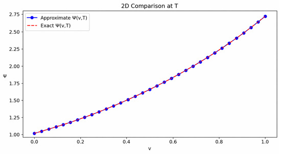
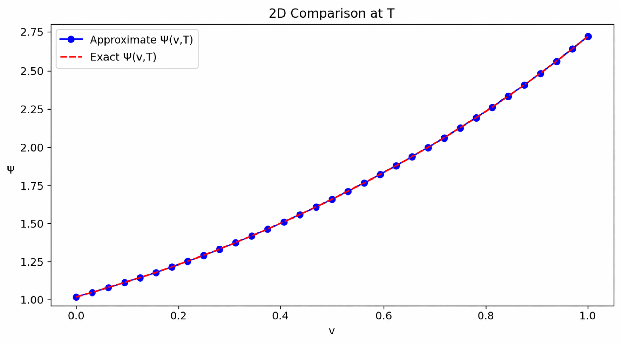
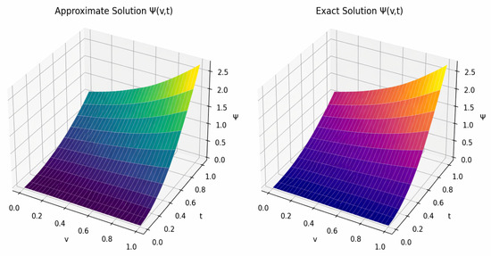
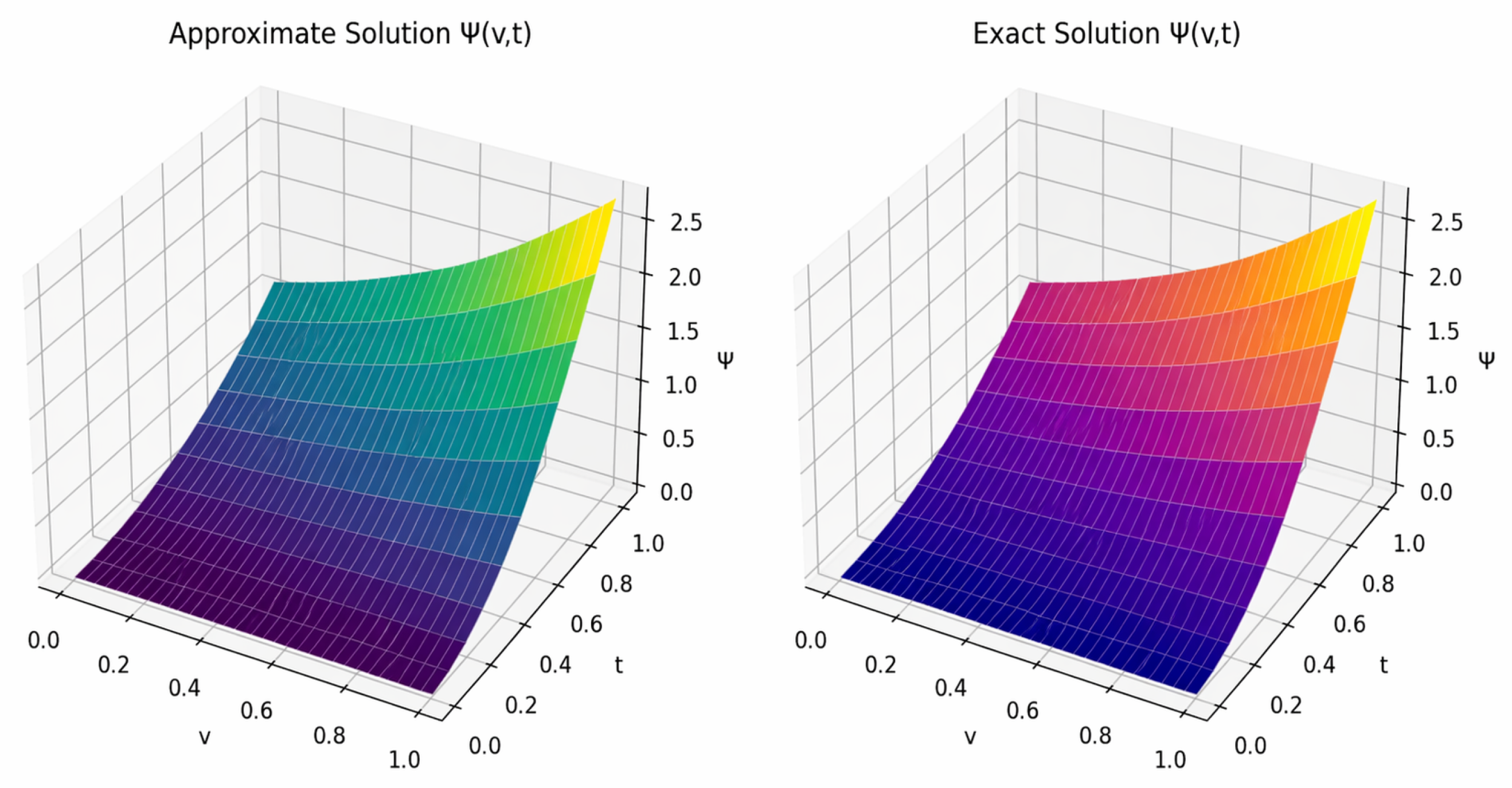
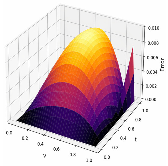
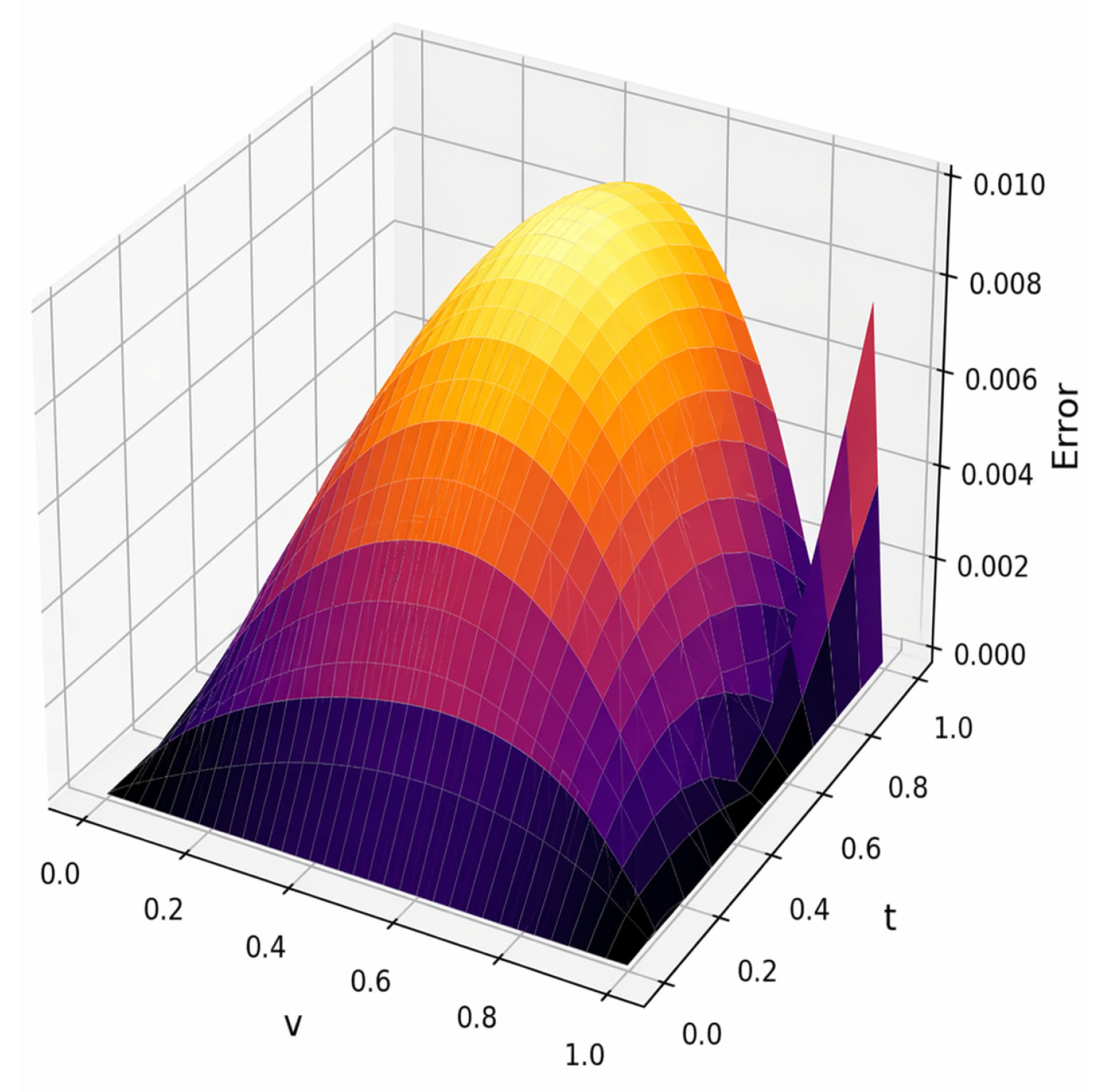
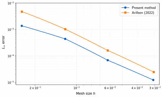
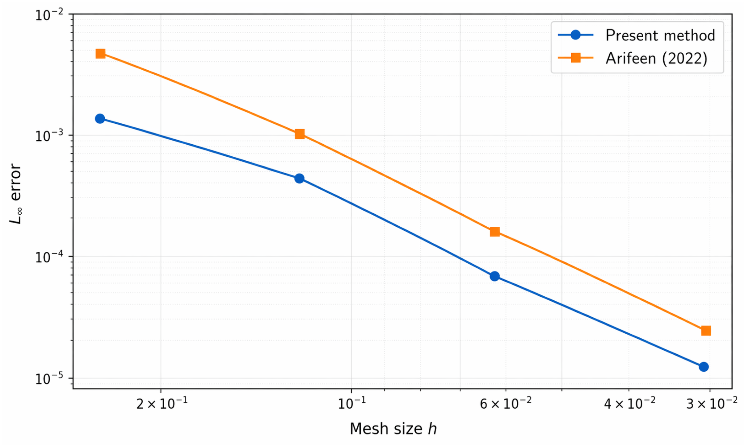
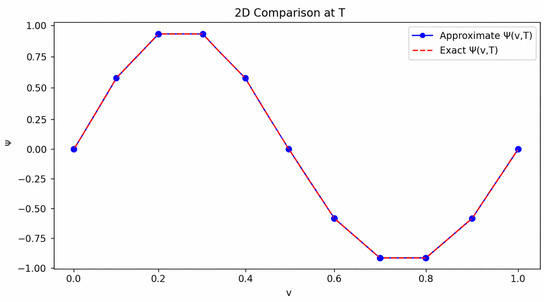
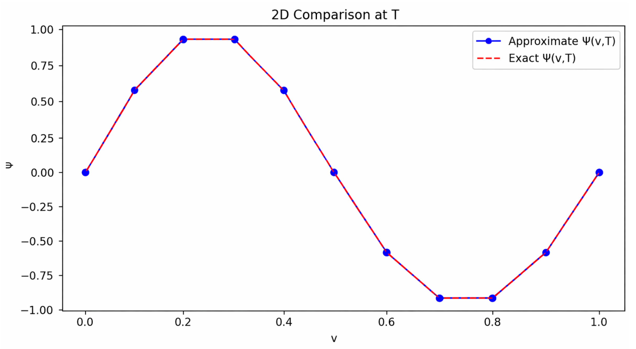
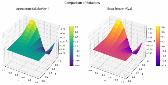
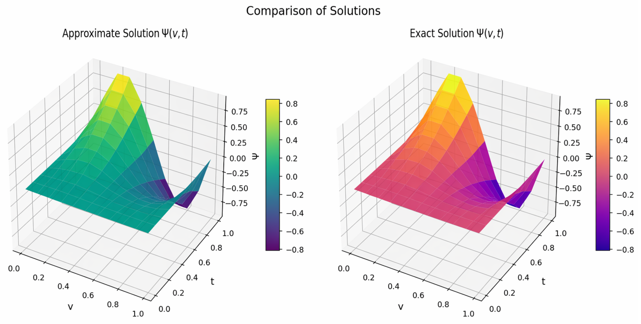
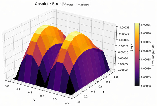
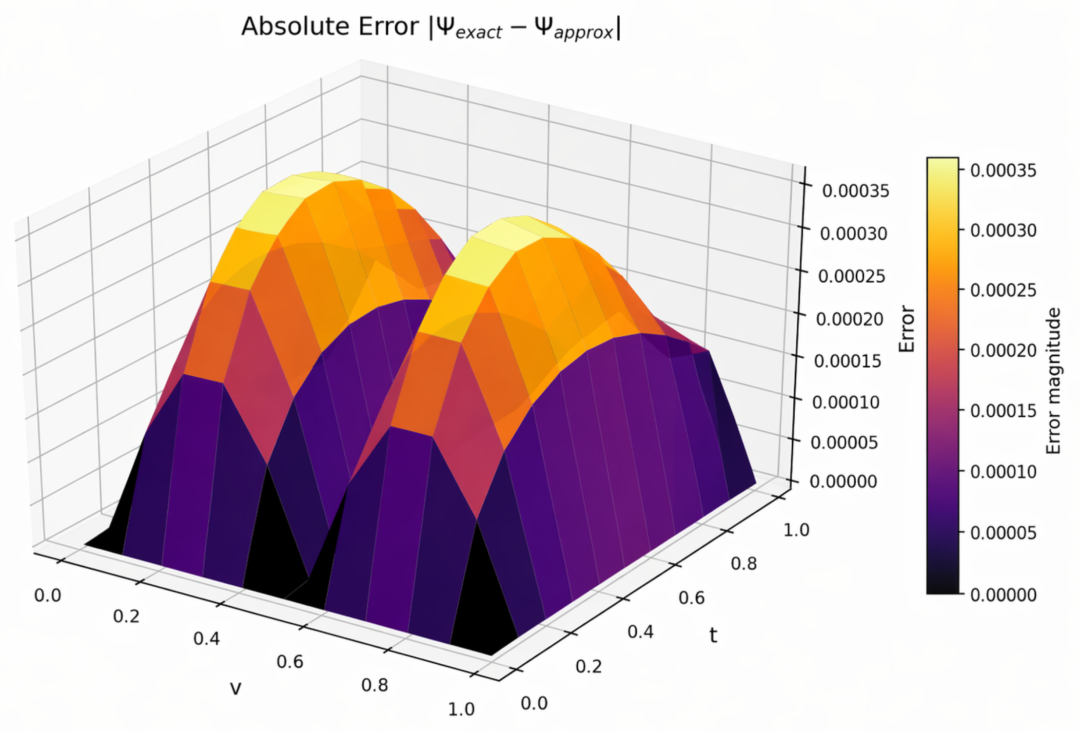
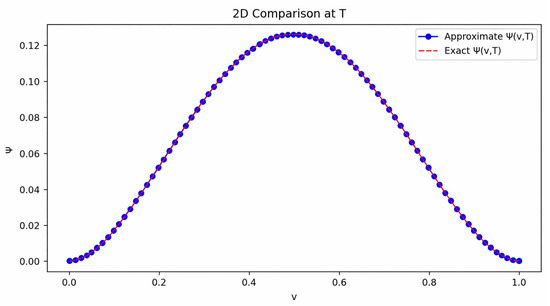
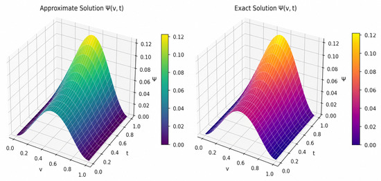
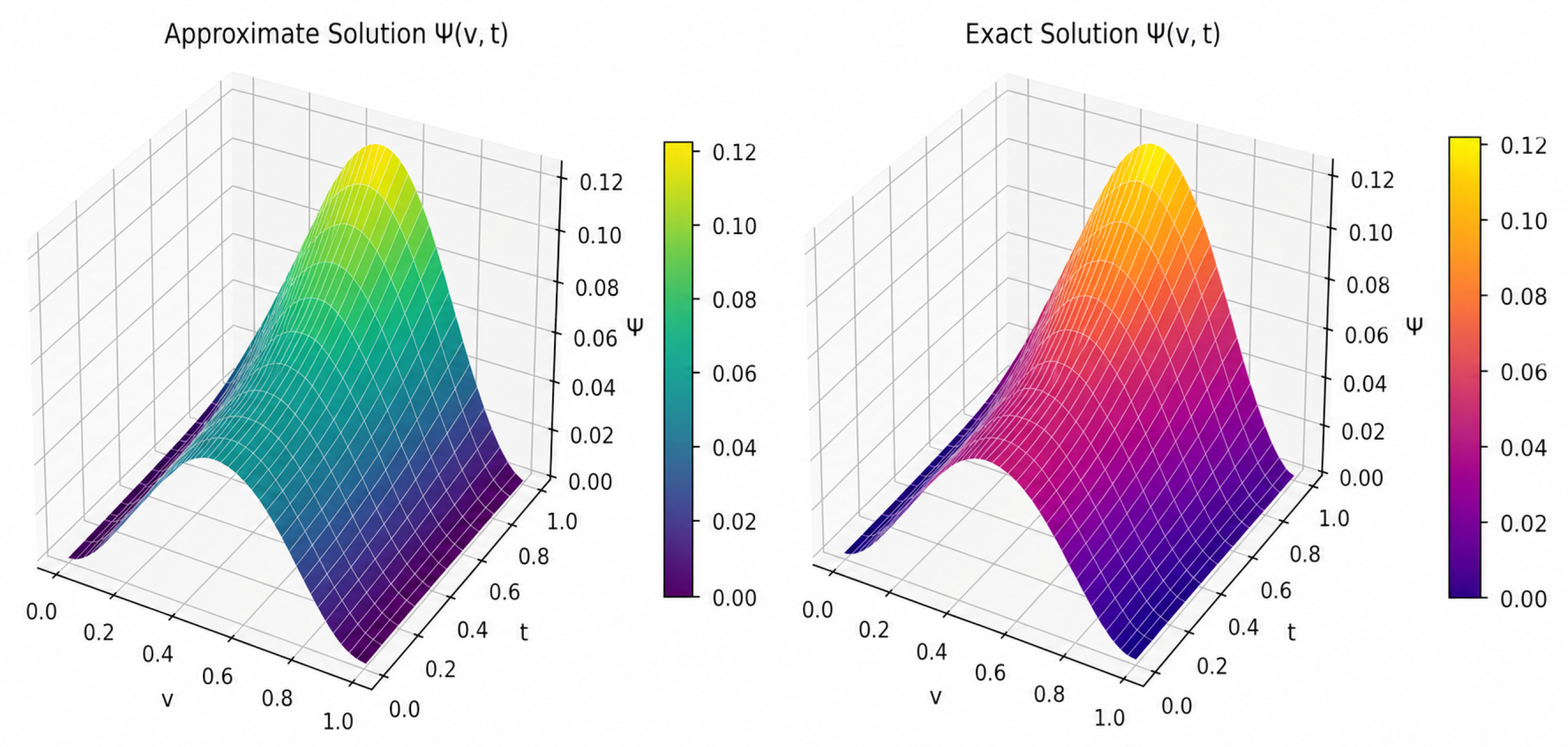
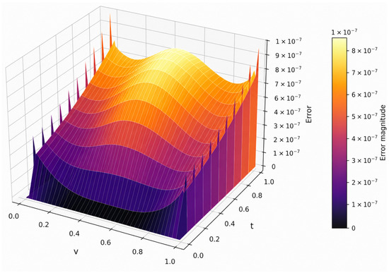
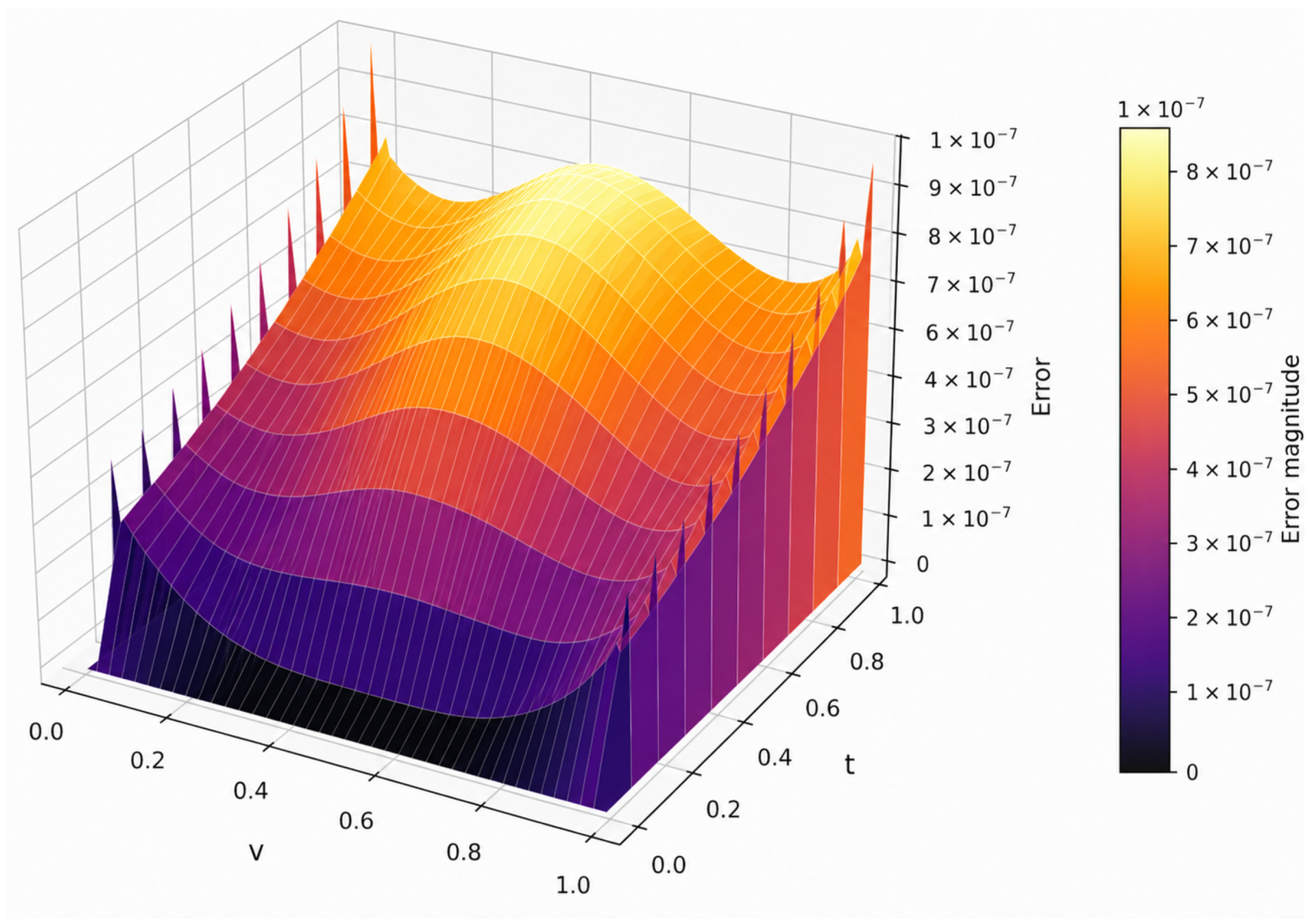
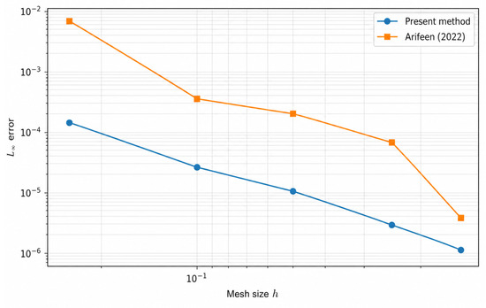
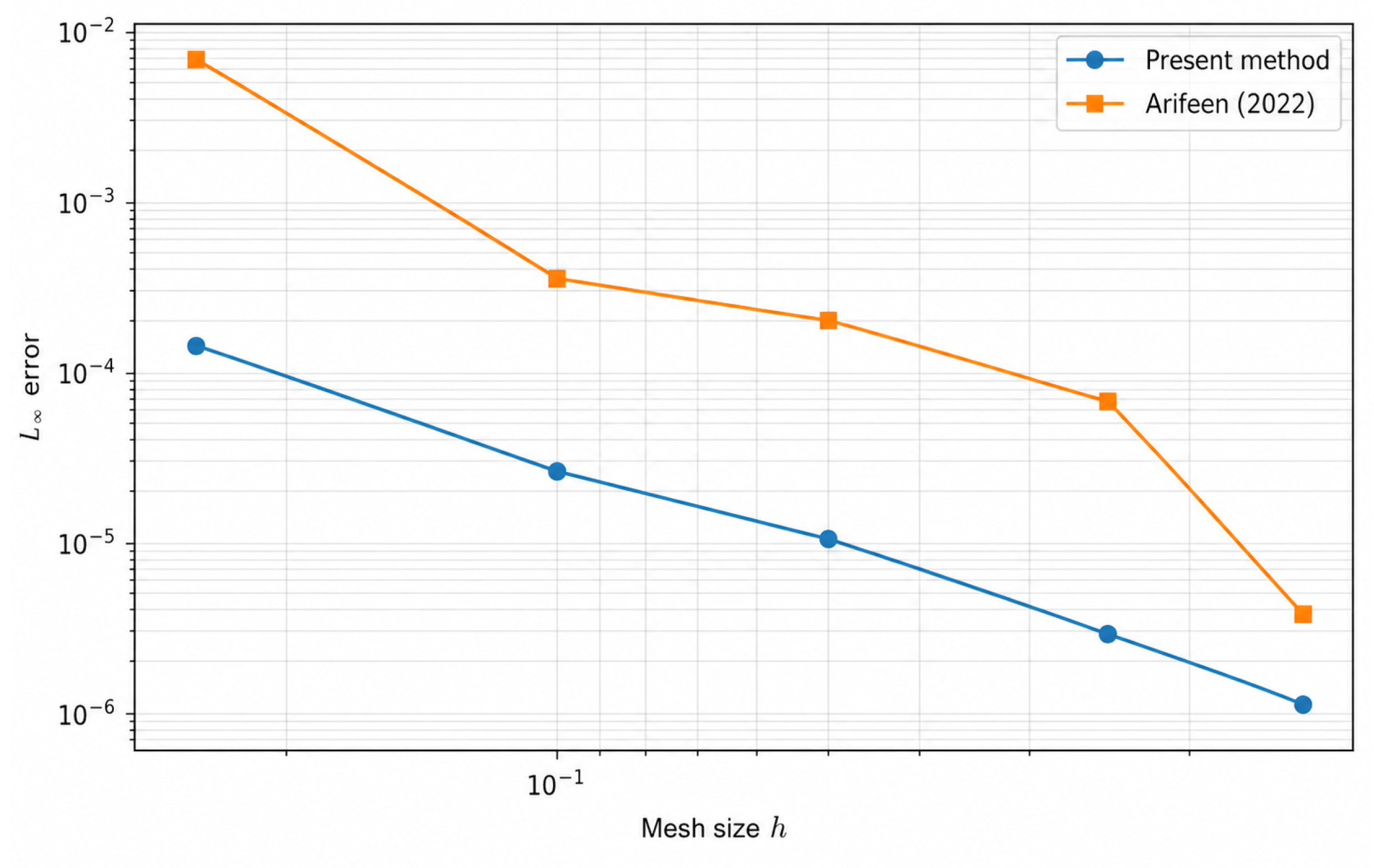
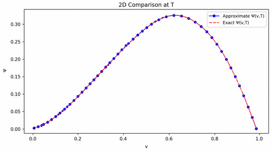
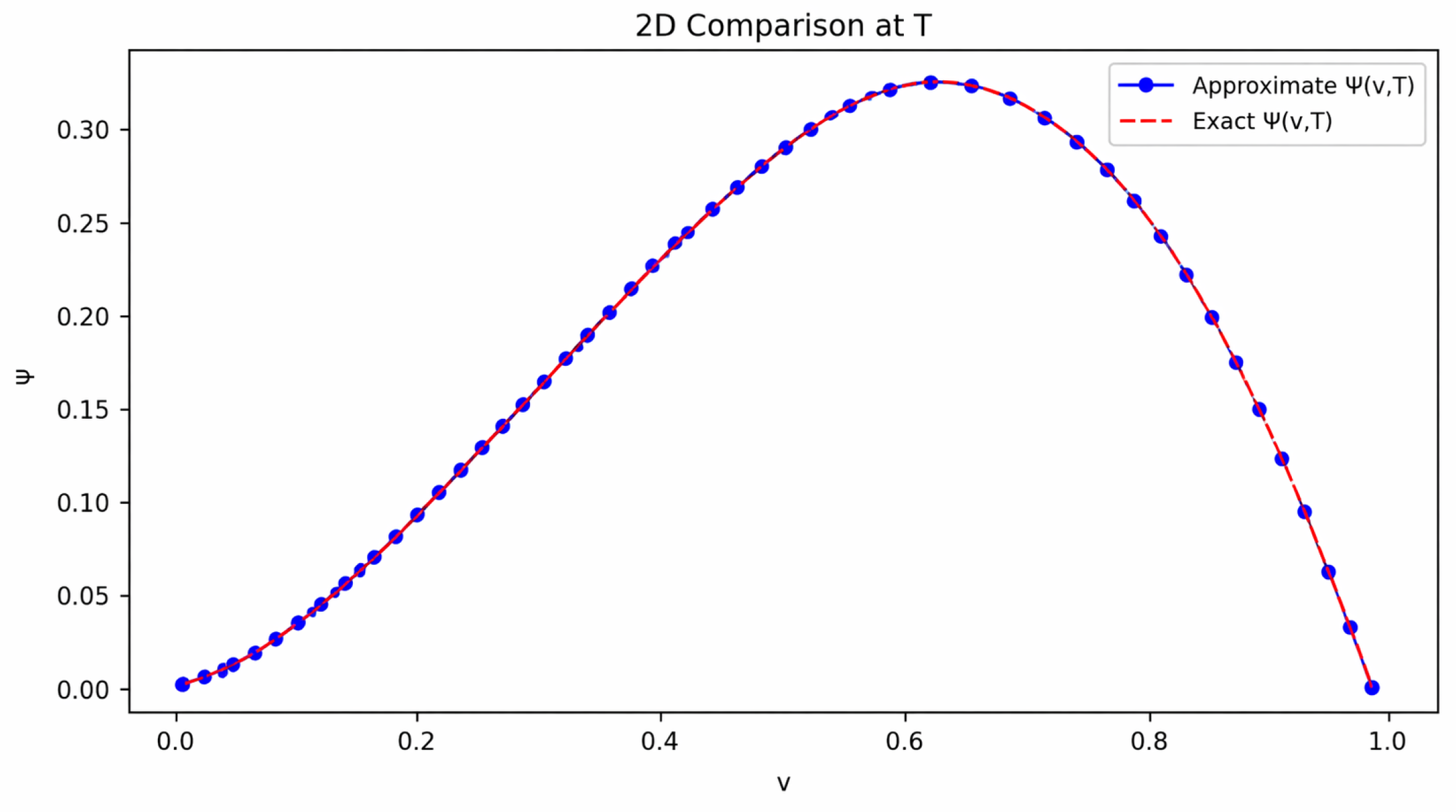
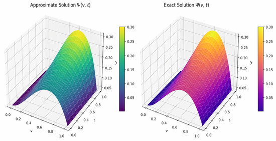
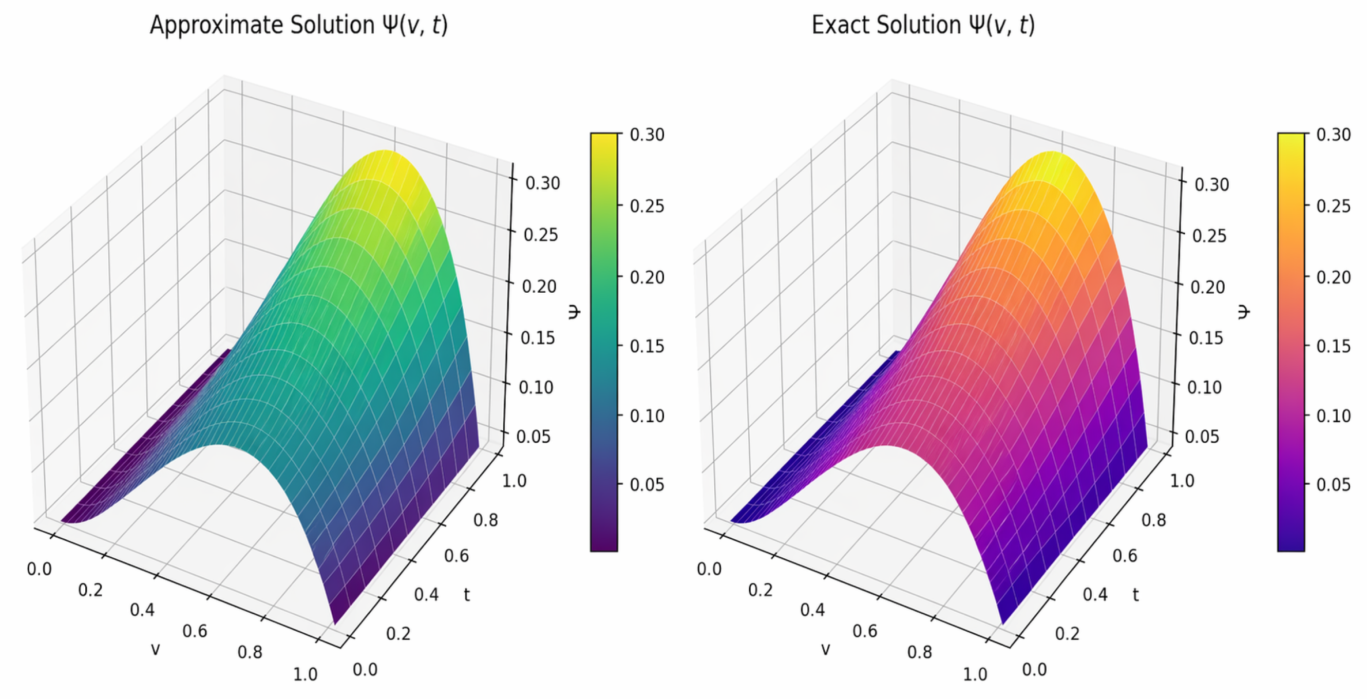
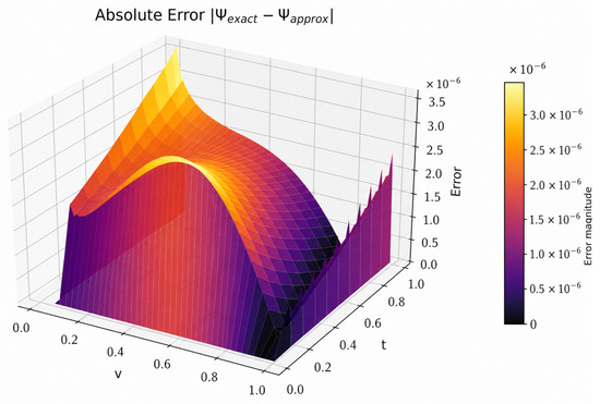
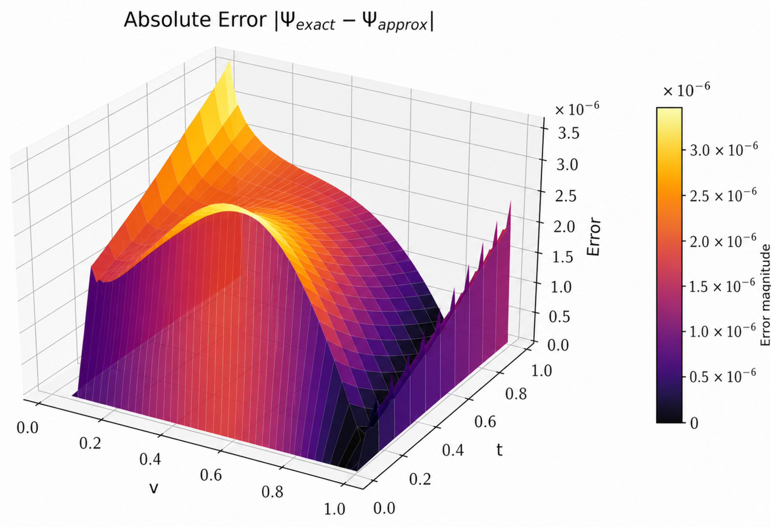
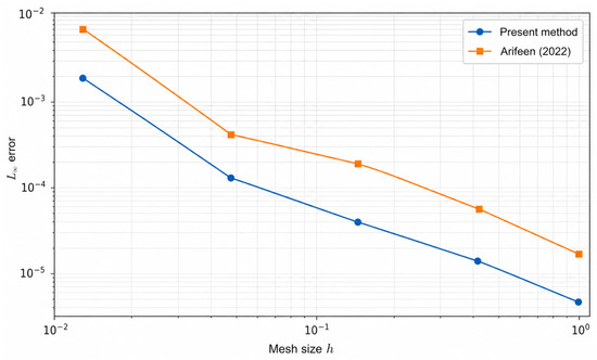
The multi-term time-fractional differential equation in Example 1 is solved using the methodology described in Section 3. The parameter values are taken as ${\mu }_1=1$, ${\mu }_2=0.85$, $\theta ={\displaystyle \frac{1}{2}}$, $a_1=1$ and $a_2=1$. The approximate solutions are computed on the interval $[0,1]$ for different choices of time step and corresponding numerical results are reported in Table 1. From the error norms, it is observed that the solution improves as the step size decreases, demonstrating the effectiveness of the proposed method. Comparing to the findings obtained from the literature (refer to [26]) the current work has produced reduced error norms for the exact same discretization parameters. Thus, we can conclude that the extended cubic B-spline Galerkin scheme is more accurate than the existing schemes. Table 1 also reports the computed rate of convergence, which is approximately of second order. Table 2 shows the effect of the parameter $\lambda$ on the $L_{\infty }$ error norm. The two-dimensional comparison between the exact and approximate solution for the given problem with $\Delta t$ = h = 0.1 is illustrated in Figure 2, while the corresponding three-dimensional representation is shown in Figure 3. The error distribution for the approximate solution is displayed in Figure 4. The log plot of the $L_{\infty }$ error against the mesh size h is shown in Figure 5. It is clear that the error consistently decreases as the mesh becomes finer, thus verifying the convergence of the proposed scheme. These graphical results confirm the excellent agreement between the numerical and exact solutions, thereby validating the proposed method.

Table 1. Absolute error analysis at different mesh sizes for Example 1.

h	$\mathit{\tau }$	${\mathit{L}}_{\mathit{\infty }}$	[26]	R.C.	R.C. [26]	CPU Time (s)
0.2500	0.0625	$2.267\times {10}^{-3}$	$5.8667\times {10}^{-3}$	—	—	0.035293
0.1250	0.0156	$1.092\times {10}^{-3}$	$1.773\times {10}^{-3}$	1.054	1.727	0.185410
0.0625	0.0039	$2.873\times {10}^{-4}$	$5.077\times {10}^{-4}$	1.926	1.804	1.506719
0.0312	0.0010	$8.746\times {10}^{-5}$	$1.407\times {10}^{-4}$	1.716	1.851	14.819878

Table 2. Effect of the extension parameter $\lambda$ on the $L_{\infty }$ error for Example 1.

h	$\mathit{\tau }$	$\mathit{\lambda }$	${\mathit{L}}_{\mathit{\infty }}$ Error
0.2500	0.0625	0.0	$6.338\times {10}^{-3}$
0.2500	0.0625	−1.5	$5.978\times {10}^{-3}$
0.2500	0.0625	−4.5	$4.621\times {10}^{-3}$
0.2500	0.0625	−5.5	$3.145\times {10}^{-3}$

Figure 2. 2D visualization of the exact and computed solutions for Example 1 when $h={\displaystyle \frac{1}{32}}$, $\tau ={\displaystyle \frac{1}{1024}}$ and $T=1$.

Figure 3. 3D visualization of the exact and computed solutions for Example 1 when $h={\displaystyle \frac{1}{32}}$, $\tau ={\displaystyle \frac{1}{1024}}$ and $T=1$.

Figure 4. 3D error distribution for Example 1 when $h={\displaystyle \frac{1}{32}}$, $\tau ={\displaystyle \frac{1}{1024}}$ and $T=1$.

Figure 5. Logarithmic comparison of the $L_{\infty }$ error with versus mesh size h for Example 1 [26].

Remark 5.

Although an optimal selection rule for λ is not available, its value is chosen based on numerical experimentation to achieve improved accuracy.

Example 2.

We consider the following two-term time-fractional differential equation:

$$\sum _{i=1}^2{a}_i{\displaystyle \frac{{\partial }^{{\mu }_i}\psi (v,t)}{\partial t^{{\mu }_i}}}={\displaystyle \frac{{\partial }^2\psi (v,t)}{\partial v^2}}+\left({\displaystyle \frac{2t^{2-{\mu }_1}}{\mathrm{\Gamma }(3-{\mu }_1)}}+{\displaystyle \frac{2t^{2-{\mu }_2}}{\mathrm{\Gamma }(3-{\mu }_2)}}\right)sin\left(2\pi v\right)+4{\pi }^2{t}^{2}sin\left(2\pi v\right).$$

(39)

with the initial condition

$$\psi (v,0)=0,v\in [0,1]$$

(40)

and the boundary conditions

$$\psi (0,t)=\psi (v,t)=0,t\in [0,1].$$

(41)

The exact solution is given by

$$\psi (v,t)=t^{2}sin\left(2\pi v\right).$$

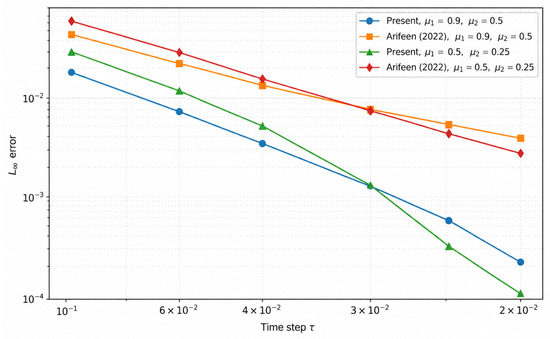
Using the numerical procedure developed in Section 3, the solution of the two-term time-fractional differential equation in Example 2 is obtained. The parameter values are chosen as $a_1=1$, $a_2=1$ and $\theta =0.5$, while the fractional orders ${\mu }_1$ and ${\mu }_2$ vary in the interval $[0,1]$ as shown in Table 3 and Table 4. The numerical solution is computed using different time step sizes while keeping the spatial step size fixed. The corresponding error analysis is presented in Table 3 and Table 4. It can be observed that the error decreases as the time step size becomes smaller, demonstrating the stability and accuracy of the proposed method. Furthermore, comparison with the results reported in [26] indicates that the present scheme provides improved accuracy. The computed convergence rates are also reported and are approximately of second order. Table 5 shows the effect of the parameter $\lambda$ on the $L_{\infty }$ error. Figure 6 and Figure 7 illustrate the comparison between the exact and numerical solutions in two-dimensional and three-dimensional forms, respectively, while Figure 8 presents the corresponding error distribution. The log plots of the $L_{\infty }$ error against the time step $\tau$ are presented for different fractional orders in Figure 9. It is obvious that the error consistently decreases as the time step becomes smaller. These graphical results demonstrate the excellent agreement between the exact and approximate solutions, thereby confirming the reliability of the proposed numerical method.

Table 3. Absolute error analysis for Example 2 with ${\mu }_1=0.9,{\mu }_2=0.5,h=0.1,\lambda =0.1$.

	${\mathit{\mu }}_1=0.9,{\mathit{\mu }}_2=0.5,\mathit{h}=0.1,\mathit{\lambda }=0.1$
$\mathit{h}$	$\mathit{\tau }$	${\mathit{L}}_{\infty }$	[26]	R.C.	R.C. [26]	CPU Time (s)
$1/10$	$1/10$	$2.573\times {10}^{-3}$	$4.705\times {10}^{-3}$	—	—	0.067628
$1/10$	$1/20$	$1.112\times {10}^{-3}$	$2.702\times {10}^{-3}$	1.211	0.8002	0.098239
$1/10$	$1/30$	$5.918\times {10}^{-4}$	$2.001\times {10}^{-3}$	0.909	0.4333	0.145499
$1/10$	$1/40$	$3.231\times {10}^{-4}$	$1.641\times {10}^{-3}$	0.873	0.2861	0.174847
$1/10$	$1/50$	$1.583\times {10}^{-4}$	$1.421\times {10}^{-3}$	1.029	0.2077	0.213621

Table 4. Absolute error analysis for Example 2 with ${\mu }_1=0.5,{\mu }_2=0.25,h=0.1,\lambda =0.25$.

	${\mathit{\mu }}_1=0.5,{\mathit{\mu }}_2=0.25,\mathit{h}=0.1,\mathit{\lambda }=0.25$
$\mathit{h}$	$\mathit{\tau }$	${\mathit{L}}_{\infty }$	[26]	R.C.	R.C. [26]	CPU Time (s)
$1/10$	$1/10$	$3.656\times {10}^{-3}$	$5.615\times {10}^{-3}$	—	—	0.070615
$1/10$	$1/20$	$1.378\times {10}^{-3}$	$2.899\times {10}^{-3}$	1.401	0.9537	0.102168
$1/10$	$1/30$	$5.966\times {10}^{-4}$	$1.971\times {10}^{-3}$	1.208	0.5566	0.145862
$1/10$	$1/40$	$2.165\times {10}^{-4}$	$1.501\times {10}^{-3}$	1.463	0.3930	0.172217
$1/10$	$1/50$	$1.017\times {10}^{-4}$	$1.217\times {10}^{-3}$	1.089	0.3026	0.207723

Table 5. Effect of the extension parameter $\lambda$ on the $L_{\infty }$ error for Example 2.

h	$\mathit{\tau }$	$\mathit{\lambda }$	${\mathit{L}}_{\mathit{\infty }}$ Error
$1/10$	$1/20$	0.0	$2.902\times {10}^{-3}$
$1/10$	$1/20$	0.05	$2.736\times {10}^{-3}$
$1/10$	$1/20$	0.08	$2.638\times {10}^{-3}$
$1/10$	$1/20$	0.5	$1.374\times {10}^{-3}$

Figure 6. 2D comparison between exact and numerical solutions for Example 2 when $h={\displaystyle \frac{1}{32}}$, $\tau ={\displaystyle \frac{1}{1024}}$ and $T=1$.

Figure 7. 3D comparison between exact and numerical solutions for Example 2 when $h={\displaystyle \frac{1}{32}}$, $\tau ={\displaystyle \frac{1}{1024}}$ and $T=1$.

Figure 8. 3D error distribution for Example 2 when $h={\displaystyle \frac{1}{32}}$, $\tau ={\displaystyle \frac{1}{1024}}$ and $T=1$.

Figure 9. Logarithmic comparison of the $L_{\infty }$ error versus time step $\tau$ for Example 2 [26].

Example 3.

Consider the following three-term time-fractional differential equation:

$$\begin{array}{cc}\hfill \sum _{i=1}^3{a}_i{\displaystyle \frac{{\partial }^{{\mu }_i}\psi (v,t)}{\partial t^{{\mu }_i}}}-{\displaystyle \frac{{\partial }^2\psi (v,t)}{\partial v^2}}& =2v^2{(1-v)}^2({\displaystyle \frac{a_1{t}^{2-{\mu }_1}}{\mathrm{\Gamma }(3-{\mu }_1)}}\hfill \\ \hfill & +{\displaystyle \frac{a_2{t}^{2-{\mu }_2}}{\mathrm{\Gamma }(3-{\mu }_2)}}+{\displaystyle \frac{a_3{t}^{2-{\mu }_3}}{\mathrm{\Gamma }(3-{\mu }_3)}})\hfill \\ \hfill & -2(6v^2-6v+1)(1+t^2).\hfill \end{array}$$

with the Initial condition

$$\psi (v,0)=v^2{(1-v)}^2,v\in [0,1]$$

and the boundary conditions

$$\psi (0,t)=\psi (1,t)=0,t\in [0,1].$$

The exact solution is given by

$$\psi (v,t)=v^2{(1-v)}^2(1+t^2).$$

In Example 3, the proposed scheme is applied over the spatial domain $[a,b]$. The parameter are chosen as the following values: $a_1=1$, $a_2=1$, $a_3=0.5$, $\theta =0.5$, ${\mu }_1=0.7$, ${\mu }_2=0.6$, ${\mu }_3=0.4$ and $\lambda =0.3$. The performance of the proposed numerical scheme is evaluated using the $L_{\infty }$ error norms reported in Table 6. It can be observed that the numerical accuracy improves as the mesh size and time step decrease. Furthermore, comparison with implicit finite difference scheme reported in [26] demonstrates that the present method produces significantly smaller errors. The computed convergence rates, also shows in Table 6, indicates that the proposed scheme achieves approximately second-order accuracy. Table 7 shows the effect of the parameter $\lambda$ on the $L_{\infty }$ error. The graphical comparison between the exact solution, the numerical approximation and the corresponding point-wise error at $\Delta t=h=0.1$ and $t=1$ is illustrated in Figure 10, Figure 11 and Figure 12. As seen in Figure 13, which displays the relationship between the $L_{\infty }$ error and the mesh width h, the convergence features of the problem in Example 3 have been represented using a log-log graph. These figures show that the numerical and analytical solutions overlap closely, confirming the accuracy and reliability of the proposed method.

Table 6. Absolute error analysis at different mesh sizes for Example 3.

h	$\mathit{\tau }$	${\mathit{L}}_{\mathit{\infty }}$	[26]	R.C.	R.C. [26]	CPU Time (s)
0.2500	0.0625	$1.803\times {10}^{-4}$	$7.308\times {10}^{-3}$	—	—	0.040473
0.1000	0.0100	$4.730\times {10}^{-5}$	$6.450\times {10}^{-4}$	1.931	3.502	0.453095
0.0500	0.0025	$1.328\times {10}^{-5}$	$4.246\times {10}^{-4}$	1.832	0.603	4.157616
0.0250	0.0063	$3.467\times {10}^{-6}$	$1.085\times {10}^{-4}$	1.938	1.967	44.846059
0.0125	0.0016	$8.825\times {10}^{-7}$	$2.746\times {10}^{-5}$	1.974	1.982	561.711480

Table 7. Effect of the extension parameter $\lambda$ on the $L_{\infty }$ error for Example 3.

h	$\mathit{\tau }$	$\mathit{\lambda }$	${\mathit{L}}_{\mathit{\infty }}$ Error
0.2500	0.0625	0.0	$5.403\times {10}^{-4}$
0.2500	0.0625	0.1	$2.801\times {10}^{-4}$
0.2500	0.0625	0.2	$1.935\times {10}^{-4}$
0.2500	0.0625	0.25	$1.891\times {10}^{-4}$

Figure 10. 2D comparison between exact and numerical solutions when $h={\displaystyle \frac{1}{80}}$, $\tau ={\displaystyle \frac{1}{6400}}$ and $T=1$ for Example 3.

Figure 11. 3D comparison between exact and numerical solutions when $h={\displaystyle \frac{1}{80}}$, $\tau ={\displaystyle \frac{1}{6400}}$ and $T=1$ for Example 3.

Figure 12. 3D error distribution when $h={\displaystyle \frac{1}{80}}$, $\tau ={\displaystyle \frac{1}{6400}}$ and $T=1$ for Example 3.

Figure 13. Logarithmic comparison of the $L_{\infty }$ error versus mesh size h for Example 3 [26].

Example 4.

Consider the following three-term time-fractional differential equation:

$$\begin{array}{cc}\hfill \sum _{i=1}^3{a}_i{\displaystyle \frac{{\partial }^{{\mu }_i}\psi (v,t)}{\partial t^{{\mu }_i}}}-{\displaystyle \frac{{\partial }^2\psi (v,t)}{\partial v^2}}& =v^{1+{\mu }_1}(1-v)\mathrm{\Gamma }({\mu }_2+{\mu }_3+1)(a_1{\displaystyle \frac{t^{{\mu }_2+{\mu }_3-{\mu }_1}}{\mathrm{\Gamma }({\mu }_2+{\mu }_3-{\mu }_1+1)}}\hfill \\ \hfill & +a_2{\displaystyle \frac{t^{{\mu }_3}}{\mathrm{\Gamma }({\mu }_3+1)}}+a_3{\displaystyle \frac{t^{{\mu }_2}}{\mathrm{\Gamma }({\mu }_2+1)}})\hfill \\ \hfill & -(1+{\mu }_1)v^{{\mu }_1-1}({\mu }_1-(2+{\mu }_1)v)(1+t^{{\mu }_2+{\mu }_3})\hfill \end{array}$$

with the initial condition

$$\psi (v,0)=v^{1+{\mu }_1}(1-v),v\in [0,1]$$

and the boundary conditions

$$\psi (0,t)=0,\psi (1,t)=0,t\in [0,1].$$

The exact solution is given by

$$\psi (v,t)=v^{1+{\mu }_1}(1-v)\left(1+t^{{\mu }_2+{\mu }_3}\right).$$

The approximate solution is computed over the spatial domain $[a,b]$ using the parameter values

$$a_1=a_3=1,a_2=0.5,\theta =0.5,{\mu }_1=0.8,{\mu }_2=0.7,{\mu }_3=0.6,\lambda =0.5.$$

The $L_{\infty }$ error norms obtained for successfully refined time steps represented in Table 8. It can be observed that the error decrease as the time step size becomes smaller, indicating the stability and efficiency of the proposed numerical scheme. Furthermore, comparison with the results reported in [26] shows that the present method provides significantly smaller errors. The computed convergence rates reported in Table 8 indicate that the scheme achieves approximately second-order accuracy. Table 9 shows the effect of the parameter $\lambda$ on the $L_{\infty }$ error. The graphical comparisons between the exact solution, the numerical approximation and the corresponding pointwise error is illustrated in Figure 14, Figure 15 and Figure 16. Figure 17 shows the logarithmic comparison of the $L_{\infty }$ error with respect to mesh refinement. A consistent reduction in error is observed, further confirming the convergence and reliability of the proposed numerical approach. These figures demonstrate an excellent agreement between the analytical and numerical solutions, confirming the effectiveness of the proposed method.

Table 8. Absolute error analysis at different mesh sizes for Example 4.

h	$\mathit{\tau }$	${\mathit{L}}_{\mathit{\infty }}$	[26]	R.C.	R.C. [26]	CPU Time (s)
0.2500	0.0625	$1.186\times {10}^{-3}$	$3.178\times {10}^{-3}$	—	—	0.037496
0.1000	0.0100	$1.512\times {10}^{-4}$	$4.758\times {10}^{-4}$	2.971	2.739	0.445019
0.0500	0.0025	$4.386\times {10}^{-5}$	$1.324\times {10}^{-4}$	1.785	1.845	4.086468
0.0250	0.0063	$1.286\times {10}^{-5}$	$3.647\times {10}^{-5}$	1.770	1.860	44.349033
0.0125	0.0016	$3.761\times {10}^{-6}$	$1.001\times {10}^{-5}$	1.774	1.865	560.430845

Table 9. Effect of the extension parameter $\lambda$ on the $L_{\infty }$ error for Example 4.

h	$\mathit{\tau }$	$\mathit{\lambda }$	${\mathit{L}}_{\mathit{\infty }}$ Error
0.2500	0.0625	0.0	$1.831\times {10}^{-3}$
0.2500	0.0625	0.1	$1.690\times {10}^{-3}$
0.2500	0.0625	0.2	$1.555\times {10}^{-3}$
0.2500	0.0625	0.4	$1.303\times {10}^{-3}$

Figure 14. 2D comparison between exact and numerical solutions when $h={\displaystyle \frac{1}{80}}$, $\tau ={\displaystyle \frac{1}{6400}}$ and $T=1$ for Example 4.

Figure 15. 3D comparison between exact and numerical solutions when $h={\displaystyle \frac{1}{80}}$, $\tau ={\displaystyle \frac{1}{6400}}$ and $T=1$ for Example 4.

Figure 16. 3D error distribution when $h={\displaystyle \frac{1}{80}}$, $\tau ={\displaystyle \frac{1}{6400}}$ and $T=1$ for Example 4.

Figure 17. Logarithmic comparison of the $L_{\infty }$ error versus mesh size h for Example 4 [26].

6. Conclusions

In this study, a numerical scheme based on extended cubic B-spline Galerkin finite element method has been developed for solving multi-term time-fractional differential equations. The temporal fractional derivatives are discretized using the Caputo definition with a finite difference approximation, while the spatial discretization is performed using extended cubic B-spline basis functions. These basis functions include a free parameter $\lambda$, which provides additional flexibility and improves the approximation capability of the method. The forcing terms are evaluated using Gauss–Legendre quadrature, which ensures accurate numerical integration. The effectiveness of the proposed scheme has been validated through several numerical tests problems involving single-, double- and triple-term time-fractional differential equations. The numerical accuracy has been assessed using the $L_2$ and $L_{\infty }$ error norms and the obtained results show excellent agreement with the corresponding exact solutions. Furthermore, the stability of the proposed method has been established through Fourier analysis, confirming its stability. Comparative studies with existing numerical approaches reported in the literature demonstrate that the proposed scheme achieves improved accuracy and convergence properties. Therefore, the extended cubic B-spline Galerkin finite element method provides an efficient and reliable numerical tool for solving multi-term time-fractional differential equations. The current research can be further developed in many ways, such as dealing with nonlinear equations, high dimensions, adaptive schemes, variable order fractional derivatives and space fractional equations. This research is ongoing and will be reported in forthcoming papers.

References

- Kulish, V.V.; Lage, J.L. Application of fractional calculus to fluid mechanics. J. Fluids Eng. 2002, 124, 803–806. [Google Scholar] [CrossRef] [Scilit]
- Tarasov, V.E. Mathematical economics: Application of fractional calculus. Mathematics 2020, 8, 660. [Google Scholar] [CrossRef] [Scilit]
- Bagley, R.L.; Torvik, P.J. A theoretical basis for the application of fractional calculus to viscoelasticity. J. Rheol. 1983, 27, 201–210. [Google Scholar] [CrossRef] [Scilit]
- Arifeen, S.U.; Haq, S.; Ali, I.; Aldosary, S.F. Galerkin approximation for multi-term time-fractional differential equations. Ain Shams Eng. J. 2024, 15, 102806. [Google Scholar] [CrossRef] [Scilit]
- Luchko, Y. Initial-boundary-value problems for the generalized multi-term time-fractional diffusion equation. J. Math. Anal. Appl. 2011, 374, 538–548. [Google Scholar] [CrossRef] [Scilit]
- Katsikadelis, J.T. Numerical solution of multiterm fractional differential equations using the matrix Mittag–Leffler functions. Mathematics 2018, 6, 7. [Google Scholar] [CrossRef] [Scilit]
- Abbas, M.; Majid, A.A.; Ismail, A.I.M.; Rashid, A. The application of cubic trigonometric B-spline to the numerical solution of the hyperbolic problems. Appl. Math. Comput. 2014, 239, 74–88. [Google Scholar] [CrossRef] [Scilit]
- Liu, F.; Meerschaert, M.M.; McGough, R.J.; Zhuang, P.; Liu, Q. Numerical methods for solving the multi-term time-fractional wave-diffusion equation. Fract. Calc. Appl. Anal. 2013, 16, 9–25. [Google Scholar] [CrossRef] [Scilit]
- Brandibur, O.; Kaslik, E. Stability properties of multi-term fractional-differential equations. Fractal Fract. 2023, 7, 117. [Google Scholar] [CrossRef] [Scilit]
- Ravi Kanth, A.S.V.; Garg, N. An implicit numerical scheme for a class of multi-term time-fractional diffusion equation. Eur. Phys. J. Plus 2019, 134, 312. [Google Scholar] [CrossRef] [Scilit]
- Ahmad, I.; Ahmad, H.; Tounthong, P.; Chu, Y.-M.; Cesarano, C. Solution of multi-term time-fractional PDE models arising in mathematical biology and physics by local meshless method. Symmetry 2020, 12, 1195. [Google Scholar] [CrossRef] [Scilit]
- Yang, X.; Wu, L. A new kind of parallel natural difference method for multi-term time fractional diffusion model. Mathematics 2020, 8, 596. [Google Scholar] [CrossRef] [Scilit]
- Zheng, M.; Liu, F.; Anh, V.; Turner, I. A high-order spectral method for the multi-term time-fractional diffusion equations. Appl. Math. Model. 2016, 40, 4970–4985. [Google Scholar] [CrossRef] [Scilit]
- Sin, C.S.; Ri, G.I.; Kim, M.C. Analytical solutions to multi-term time-space Caputo-Riesz fractional diffusion equations on an infinite domain. Adv. Differ. Equ. 2017, 2017, 306. [Google Scholar] [CrossRef] [Scilit]
- Daftardar-Gejji, V.; Bhalekar, S. Boundary value problems for multi-term fractional differential equations. J. Math. Anal. Appl. 2008, 345, 754–765. [Google Scholar] [CrossRef] [Scilit]
- Li, Z.; Liu, Y.; Yamamoto, M. Initial-boundary value problems for multi-term time-fractional diffusion equations with positive constant coefficients. Appl. Math. Comput. 2015, 257, 381–397. [Google Scholar] [CrossRef] [Scilit]
- Hussain, M.; Haq, S. Weighted meshless spectral method for the solutions of multi-term time fractional advection diffusion problems arising in heat and mass transfer. Int. J. Heat Mass Transf. 2019, 129, 1305–1316. [Google Scholar] [CrossRef] [Scilit]
- Dehghan, M.; Safarpoor, M.; Abbaszadeh, M. Two high-order numerical algorithms for solving the multi-term time fractional diffusion-wave equations. J. Comput. Appl. Math. 2015, 290, 174–195. [Google Scholar] [CrossRef] [Scilit]
- Ren, J.; Sun, Z.-Z. Efficient and stable numerical methods for multi-term time fractional sub-diffusion equations. East Asian J. Appl. Math. 2014, 4, 242–266. [Google Scholar] [CrossRef] [Scilit]
- Edwards, J.T.; Ford, N.J.; Simpson, A.C. The numerical solution of linear multi-term fractional differential equations: Systems of equations. J. Comput. Appl. Math. 2002, 148, 401–418. [Google Scholar] [CrossRef] [Scilit]
- Brandibur, O.; Kaslik, E. Stability analysis of multi-term fractional-differential equations with three fractional derivatives. J. Math. Anal. Appl. 2021, 495, 124751. [Google Scholar] [CrossRef] [Scilit]
- Bhrawy, A.H.; Baleanu, D.; Assas, L.M. Efficient generalized Laguerre-spectral methods for solving multi-term fractional differential equations on the half line. J. Vib. Control 2013, 20, 1000–1015. [Google Scholar] [CrossRef] [Scilit]
- Zeng, F.; Zhang, Z.; Karniadakis, G.E. Second-order numerical methods for multi-term fractional differential equations: Smooth and non-smooth solutions. Comput. Methods Appl. Mech. Eng. 2017, 327, 478–502. [Google Scholar] [CrossRef] [Scilit]
- Gazi Karakoc, S.B.; Geyikli, T. Petrov-Galerkin finite element method for solving the MRLW equation. Math. Sci. 2013, 7, 25. [Google Scholar] [CrossRef] [Scilit]
- Esen, A.; Taşbozan, O. Numerical solution of time fractional Burgers equation by cubic B-spline finite elements. Mediterr. J. Math. 2016, 13, 1325–1337. [Google Scholar] [CrossRef] [Scilit]
- Arifeen, S.U.; Haq, S.; Golkarmanesh, F. Computational study of multiterm time-fractional differential equation using cubic B-spline finite element method. Complexity 2022, 2022, 3160725. [Google Scholar] [CrossRef] [Scilit]
- Jin, B.; Lazarov, R.; Liu, Y.; Zhou, Z. The Galerkin finite element method for a multi-term time-fractional diffusion equation. J. Comput. Phys. 2015, 281, 825–843. [Google Scholar] [CrossRef] [Scilit]
- Wang, Y.; Li, T.; Zhao, Y. The finite difference method and analysis for simulating the unsteady generalized Maxwell fluid with a multi-term time fractional derivative. Fractal Fract. 2024, 8, 136. [Google Scholar] [CrossRef] [Scilit]
- Delkhosh, M.; Parand, K. A new computational method based on fractional Lagrange functions to solve multi-term fractional differential equations. Numer. Algorithms 2021, 88, 729–766. [Google Scholar] [CrossRef] [Scilit]
- Abu Arqub, O.; Tayebi, S.; Baleanu, D.; Osman, M.S.; Mahmoud, W.; Alsulami, H. A numerical combined algorithm in cubic B-spline method and finite difference technique for the time-fractional nonlinear diffusion wave equation with reaction and damping terms. Results Phys. 2022, 41, 105912. [Google Scholar] [CrossRef] [Scilit]
- Rahman, G.U.; Ahmad, D.; Gómez-Aguilar, J.F.; Agarwal, R.P.; Ali, A. Study of Caputo fractional derivative and Riemann–Liouville integral with different orders and its application in multi-term differential equations. Math. Methods Appl. Sci. 2025, 48, 1464–1502. [Google Scholar] [CrossRef] [Scilit]
- Abd-Elhameed, W.M.; Alsuyuti, M.M. Numerical treatment of multi-term fractional differential equations via new kind of generalized Chebyshev polynomials. Fractal Fract. 2023, 7, 74. [Google Scholar] [CrossRef] [Scilit]
- Pata, V.; Siryk, S.V.; Vasylyeva, N. Multi-term fractional linear equations modeling oxygen subdiffusion through capillaries. Appl. Anal. 2026, 105, 659–697. [Google Scholar] [CrossRef] [Scilit]
- Santra, S. Analysis of a higher-order scheme for multi-term time-fractional integro-partial differential equations with multi-term weakly singular kernels. Numer. Algorithms 2025, 99, 1649–1695. [Google Scholar] [CrossRef] [Scilit]
- Mani, G.; Ganesh, P.; Chidhambaram, K.; Aljohani, S.; Mlaiki, N. Existence and uniqueness solutions of multi-term delay Caputo fractional differential equations. Int. J. Anal. Appl. 2024, 22, 171. [Google Scholar] [CrossRef] [Scilit]
Disclaimer/Publisher’s Note: The statements, opinions and data contained in all publications are solely those of the individual author(s) and contributor(s) and not of MDPI and/or the editor(s). MDPI and/or the editor(s) disclaim responsibility for any injury to people or property resulting from any ideas, methods, instructions or products referred to in the content. |
© 2026 by the authors. Licensee MDPI, Basel, Switzerland. This article is an open access article distributed under the terms and conditions of the Creative Commons Attribution (CC BY) license.