Qualitative Analysis and Numerical Simulations of γ-Hilfer Fractional Stochastic Dynamical Systems

Abstract

This study presents findings on the existence, uniqueness, averaging principle, and numerical solutions for fractional stochastic systems influenced by both Brownian motion and Poisson jumps within the pth-moment framework. While most existing results for fractional stochastic differential equations are derived using the mean-square approach, this research offers results in the more general pth-moment framework, enhancing applicability. The results are derived using the $\gamma$-Hilfer fractional derivative, a generalized operator defined in relation to another function. This operator enables the memory effect to vary according to a nonlinear time scale. The main motivation behind this work is that there is no research work on $\gamma$-Hilfer fractional stochastic systems with standard Brownian motion and Poisson jumps regarding existence, uniqueness, and averaging principles in the pth-moment.

1. Introduction

The $\gamma$-Hilfer fractional derivative ($\gamma$-HFrD) is a generalized fractional operator defined with respect to another function $\gamma$, allowing the memory effect to depend on a nonlinear time scale. It unifies several fractional derivatives, including the Riemann–Liouville and Caputo types, and provides a flexible framework for modeling systems with nonlocal and hereditary behavior.

Definition 1.

Let $\eta >0$ and $\gamma \in C^1(I,\mathbb{R})$ be strictly increasing. For $u\in L^1(I,\mathbb{R})$, the left-sided fractional integral of order η with respect to γ is defined by [1]

$${\mathcal{I}}_{a^{+}}^{\eta ;\gamma }u\left(t\right)={\displaystyle \frac{1}{\Gamma \left(\eta \right)}}{\int }_a^t{\left(\gamma \left(t\right)-\gamma \left(s\right)\right)}^{\eta -1}{\gamma }^{\prime }\left(s\right)u\left(s\right)ds,t>a.$$

(1)

Remark 1.

The above operator generalizes the classical Riemann–Liouville fractional integral by replacing the standard time variable with a nonlinear function $\gamma \left(t\right)$.

Definition 2.

Let $n\in \mathbb{N}$ be such that $n-1<\eta <n$, and let $\gamma \in C^n(I,\mathbb{R})$ be strictly increasing. For $u\in C^n(I,\mathbb{R})$, the left-sided Caputo-type fractional derivative of order η with respect to γ is defined by [2]

$${}^{C}D_{a^{+}}^{\eta ;\gamma }u\left(t\right)={\displaystyle \frac{1}{\Gamma (n-\eta )}}{\int }_a^t{\left(\gamma \left(t\right)-\gamma \left(s\right)\right)}^{n-\eta -1}{D}_{\gamma }^{n}u\left(s\right){\gamma }^{\prime }\left(s\right)ds,t>a,$$

where

$$D_{\gamma }^{n}u\left(t\right)={\left({\displaystyle \frac{1}{{\gamma }^{\prime }\left(t\right)}}{\displaystyle \frac{d}{dt}}\right)}^{n}u\left(t\right).$$

Remark 2.

The operator $D_{\gamma }^n$ represents differentiation with respect to the function $\gamma \left(t\right)$ rather than the standard variable t. Hence, the above derivative can be interpreted as a Caputo-type fractional operator defined on a nonlinear time scale.

Definition 3.

Let $n\in \mathbb{N}$ satisfy $n-1<\eta <n$ and let $\vartheta \in [0,1]$. Under the same assumptions on γ, the left-sided Hilfer-type fractional derivative of order η and type ϑ with respect to γ is defined by [3]

$${}^{\mathcal{H}}D_{a^{+}}^{\eta ,\vartheta ,\gamma }u\left(t\right)={\mathcal{I}}_{a^{+}}^{\vartheta (n-\eta );\gamma }{\left({\displaystyle \frac{1}{{\gamma }^{\prime }\left(t\right)}}{\displaystyle \frac{d}{dt}}\right)}^n{\mathcal{I}}_{a^{+}}^{(1-\vartheta )(n-\eta );\gamma }u\left(t\right),t>a.$$

Remark 3.

The parameter $\vartheta \in [0,1]$ interpolates between different types of fractional derivatives. Specifically, $\vartheta =0$ corresponds to the γ-Riemann–Liouville type derivative, while $\vartheta =1$ yields the γ-Caputo type derivative.

Remark 4.

For the fundamental case $0<\eta <1$ (i.e., $n=1$), the above operators simplify significantly. In particular, the γ-Hilfer fractional derivative reduces to

$${}^{\mathcal{H}}D_{a^{+}}^{\eta ,\vartheta ,\gamma }u\left(t\right)={\mathcal{I}}_{a^{+}}^{\vartheta (1-\eta );\gamma }\left(\frac{1}{{\gamma }^{\prime }\left(t\right)}\frac{d}{dt}\right){\mathcal{I}}_{a^{+}}^{(1-\vartheta )(1-\eta );\gamma }u\left(t\right).$$

This case is frequently used in applications and highlights the role of the parameter ϑ.

Remark 5.

If $\gamma \left(t\right)=t$, then all the above operators reduce to the classical Riemann–Liouville, Caputo, and Hilfer fractional derivatives.

Lemma 1.

Let $u\in C^n(I,\mathbb{R})$, with $0\le \vartheta \le 1$ and $n-1<\eta <n$. Define [3]

$$\rho =\eta +\vartheta (n-\eta ).$$

Then the following composition formula holds:

$${\mathcal{I}}_{a^{+}}^{\eta ;\gamma }{}^{\mathcal{H}}D_{a^{+}}^{\eta ,\vartheta ,\gamma }u\left(t\right)=u\left(t\right)-\sum _{k=0}^{n-1}{\displaystyle \frac{{\left(\gamma \left(t\right)-\gamma \left(a\right)\right)}^{\rho -k-1}}{\Gamma (\rho -k)}}{D}_{\gamma }^k\left({\mathcal{I}}_{a^{+}}^{(1-\vartheta )(n-\eta );\gamma }u\right)\left(a\right).$$

(2)

Remark 6.

The above result establishes the inverse relationship between the γ-fractional integral and the γ-Hilfer derivative. It shows that the fractional integral of the Hilfer-type derivative recovers the original function up to correction terms involving generalized initial values.

Fractional stochastic differential equations (FSDEs) that incorporate both Brownian motion and Poisson jump noise offer an advanced framework for modeling systems that exhibit memory effects and stochastic fluctuations. In this context, the Brownian motion component accounts for continuous, minor fluctuations, while the compound Poisson process addresses significant, sudden shocks of varying magnitudes. This integrated approach serves as a powerful mathematical tool for understanding systems affected by the interaction of non-Markovian memory, diffuse randomness, and abrupt changes.

Fractional stochastic systems driven by standard Brownian motion and Poisson jumps have numerous practical applications, particularly in economics. They can effectively model economic growth processes that exhibit long-memory dynamics, wherein past investment decisions and shocks continuously affect present output. Poisson jumps highlight the speed of economic changes in response to policy shifts, financial crises, or market disruptions. These models also enable monitoring of inflation and interest rate fluctuations over time. For instance, they illustrate gradual changes in rates that can accelerate dramatically due to global events or government monetary announcements. In labor economics, these systems reflect variations in job markets over time, influenced by long-term trends as well as sudden layoffs or hiring bursts. Financial institutions, including banks, utilize fractional stochastic models to assess how enduring trends and sudden shocks, such as credit defaults or liquidity crises, will impact their operations. Such models enhance our understanding of dynamic economies that are subject to continuous change and significant, abrupt events.

Existence and uniqueness (Ex-Un) of solutions are fundamental principles in any mathematical model, ensuring that the system’s behavior is distinctly characterized and predictable. Establishing existence confirms the existence of a solution to the system, while uniqueness ensures that this solution is the sole one that aligns with the specified initial conditions. This clarity keeps system dynamics from being unclear, which is important for both theoretical analysis and numerical simulations.

The averaging principle (Av-Pr) for FSDEs provides a structured methodology for comprehending the temporal dynamics of intricate systems, especially concerning memory effects and stochastic perturbations. This principle helps us describe the system more accurately because it averages out terms that change quickly. It keeps important features of both fractional-order memory and stochastic events, like Poisson jumps and Brownian motion. By applying this concept to FSDEs, we can gain insights into the temporal evolution of systems influenced by stochastic processes and fractional dynamics. It also gives you a good starting point for making reduced-order models that keep important statistical and dynamic properties. This method is very useful for studying systems that are hard to study directly or to simulate numerically in the full fractional stochastic context.

As the Ex-Un of solutions is an important issue in the theory of FSDEs. In their investigation of neutral FSDEs with infinite delay, Sakthivel et al. [4] discovered stability properties and existence results. More generally, Ex-Un results for nonlinear FSDEs driven by Brownian motion have been obtained by combining fixed-point arguments with stochastic analytical methods; see, for instance [5,6,7,8]. These papers draw attention to the extra mathematical challenges brought about by the interaction of stochastic disturbances and fractional memory.

Numerous stability concepts for FSDEs have been thoroughly examined in addition to well-posedness. Particularly crucial for comprehending how sensitive stochastic systems are to perturbations are mean-square stability and higher-moment stability. Refs. [9,10,11,12] developed adequate criteria guaranteeing mean-square and higher-moment stability for a number of fractional stochastic model classes in this way.

In recent years, the Av-Pr and controllability have also attracted significant attention. Several notable results concerning averaging for fractional stochastic systems were obtained in [13,14,15]. Likewise, controllability properties of FSDEs, especially for systems involving delays, neutral terms, and nonlocal conditions, have been investigated extensively; see [16,17].

The following is a summary of the main contributions of this study:

• To the best of my knowledge, there is no research on $\gamma$-Hilfer fractional stochastic systems with standard Brownian motion and Poisson jumps that addresses existence, uniqueness, and Av-Pr in the pth moment.
• Most existing results on existence, uniqueness, and the Av-Pr for fractional stochastic systems have been established under standard Brownian motion. In this work, we extend these results to systems driven by both Brownian motion and Poisson jumps.
• Most existing results for FSDEs are derived in the mean-square sense. In contrast, this work presents results in the more general pth moment, providing broader applicability.
• All results are based on the $\gamma$-HFrD, a generalized fractional operator that encompasses several fractional operators.

We study the following FSDEs with delay:

$$\left\{\begin{array}{c}{}^{\mathcal{H}}D_{0^{+}}^{\eta ,\vartheta ,\gamma }\mathcal{Z}\left(t\right)=F_1(t,\mathcal{Z}\left(t\right),\mathcal{Z}\left(t-\varphi \right))+F_2(t,\mathcal{Z}\left(t\right),\mathcal{Z}\left(t-\varphi \right)){\displaystyle \frac{d\mathrm{w}\left(t\right)}{dt}}\hfill \\ +{\displaystyle \frac{{\int }_{\mathrm{V}}\mathrm{G}(t,\mathcal{Z}\left(t\right),\mathcal{Z}(t-\varphi ),\varsigma )\tilde{N}(dt,d\varsigma )}{dt}},t\in \mathrm{Q}=[0,\mathcal{X}],\hfill \\ \mathcal{Z}\left(t\right)=\mathrm{v}\left(t\right),-\varphi \le t\le 0,\hfill \end{array}\right.$$

(3)

here, $\mathcal{Z}\left(t\right)\in {\mathcal{R}}^{\mathrm{a}}$ denotes the state vector, modeled as a stochastic process. ${}^{\mathcal{H}}D_{0^{+}}^{\eta ,\vartheta ,\gamma }$ denotes the $\gamma$-HFrD of order $\eta \in (0,1)$ with parameter $\gamma >0$. $\varphi \in {\mathcal{R}}^{+}$ is the delay time, and $\mathrm{v}\left(t\right):[-\varphi ,0]\to {\mathcal{R}}^{\mathrm{a}}$ is continuous.

The following mappings are measurable and continuous:

$$\begin{array}{cc}\hfill F_1& :[0,\mathcal{X}]\times {\mathcal{R}}^{\mathrm{a}}\times {\mathcal{R}}^{\mathrm{a}}⟶{\mathcal{R}}^{\mathrm{a}},\hfill \\ \hfill F_2& :[0,\mathcal{X}]\times {\mathcal{R}}^{\mathrm{a}}\times {\mathcal{R}}^{\mathrm{a}}⟶{\mathcal{R}}^{\mathrm{a}\times \mathrm{s}},\hfill \\ \hfill \mathrm{G}& :[0,\mathcal{X}]\times {\mathcal{R}}^{\mathrm{a}}\times {\mathcal{R}}^{\mathrm{a}}\times \mathrm{V}⟶{\mathcal{R}}^{\mathrm{a}}.\hfill \end{array}$$

Furthermore, $\mathrm{w}\left(t\right)$ denotes an $\mathrm{s}$-dimensional Brownian motion defined over the probability space $(\Omega ,\mathcal{F},\mathbb{P})$. Consider $(\mathrm{V},\Phi ,\lambda (d\varsigma \left)\right)$ as a $\sigma$-finite measurable space. Denote by $\aleph (t,d\varsigma )$ the counting measure of a stationary Poisson point process ${\mathrm{p}}_t$ on $\mathrm{V}$. The compensated Poisson random measure $\tilde{N}$ is defined as

$$\tilde{N}(t,d\varsigma )=\aleph (t,d\varsigma )-t\lambda \left(d\varsigma \right).$$

The paper is structured as follows: Section 2 presents essential preliminaries on fractional calculus, stochastic analysis, and functional spaces. Section 3 addresses the Ex-Un of the proposed system. The Av-Pr is investigated in Section 4. Numerical approximations and simulation results based on a Euler–Maruyama approach are provided in Section 5. Finally, concluding remarks and potential directions for future research are discussed in Section 6 and Section 7, respectively.

2. Preliminaries

This section collects the fundamental definitions, notation, and hypotheses required for the subsequent analysis.

Definition 4.

We denote by $\mathcal{Y}={\mathrm{L}}^p(\Omega ,\mathcal{F},\mathbb{P})$ the space of ${\mathcal{F}}_t$-measurable, a-integrable functions $\mathcal{Z}={({\mathcal{Z}}_1,{\mathcal{Z}}_2,\dots ,{\mathcal{Z}}_a)}^T:\Omega \to {\mathbb{R}}^a$ satisfying

$${\parallel \mathcal{Z}\parallel }_p={\left({\sum }_{i=1}^a\mathrm{E}{|{\mathcal{Z}}_i|}^p\right)}^{\frac{1}{p}},$$

where $\mathrm{E}$ denotes the expectation with respect to $\mathbb{P}$.

A stochastic process $\mathcal{Z}:[0,\mathcal{X}]\to {\mathrm{L}}^p(\Omega ,\mathcal{F},\mathbb{P})$ that satisfies the required measurability conditions is called $\mathbb{F}$-adapted if $\mathcal{Z}\left(t\right)\in \mathcal{Y}$ for every $t\in [0,\mathcal{X}]$. For any initial value $\mathcal{Z}\left(0\right)$, such an $\mathbb{F}$-adapted process $\mathcal{Z}$ is a solution of (3) whenever condition (4) holds.

$$\begin{array}{c}\hfill \mathcal{Z}\left(t\right)=\left\{\begin{array}{cc}{\displaystyle \frac{{(\gamma \left(t\right)-\gamma \left(0\right))}^{(1-\eta )(\vartheta -1)}}{\Gamma \left(\vartheta \right(1-\eta )+\eta )}\mathcal{Z}\left(0\right)+{\displaystyle \frac{1}{\Gamma \left(\eta \right)}}{\int }_0^t{(\gamma \left(t\right)-\gamma \left(\varpi \right))}^{\eta -1}{F}_1(\varpi ,\mathcal{Z}\left(\varpi \right),\mathcal{Z}(\varpi -\varphi )){\gamma }^{\prime }\left(\varpi \right)d\varpi }\hfill & \\ {\displaystyle +{\displaystyle \frac{1}{\Gamma \left(\eta \right)}}{\int }_0^t{(\gamma \left(t\right)-\gamma \left(\varpi \right))}^{\eta -1}{F}_2\left(\varpi ,\mathcal{Z}\left(\varpi \right),\mathcal{Z}(\varpi -\varphi )\right){\gamma }^{\prime }\left(\varpi \right)d\mathrm{w}\left(\varpi \right)}\hfill & \\ {\displaystyle +{\displaystyle \frac{1}{\Gamma \left(\eta \right)}}{\int }_0^t{(\gamma \left(t\right)-\gamma \left(\varpi \right))}^{\eta -1}{\gamma }^{\prime }\left(\varpi \right){\int }_{\mathrm{V}}\mathrm{G}(\varpi ,\mathcal{Z}\left(\varpi \right),\mathcal{Z}(\varpi -\varphi ),\varsigma )\tilde{N}(d\varpi ,d\varsigma ),}\hfill & ,\hfill \\ \mathcal{Z}\left(t\right)=\mathrm{v}\left(t\right),-\varphi \le t\le 0.\hfill & \end{array}\right.\end{array}$$

(4)

For $F_1$, $F_2$, and $\mathrm{G}$, we make the following assumptions: $\left({\mathbb{H}}_1\right)$ When $\forall {\mathfrak{c}}_1,{\mathfrak{c}}_2,{\mathfrak{c}}_3,{\mathfrak{c}}_4\in {\mathcal{R}}^{\mathrm{a}}$ there are ${\mathcal{U}}_1$, ${\mathcal{U}}_2$, and ${\mathcal{U}}_3$ such as

$$\parallel F_1(t,{\mathfrak{c}}_1,{\mathfrak{c}}_2)-F_1(t,{\mathfrak{c}}_3,{\mathfrak{c}}_4){\parallel }_p^p\le {\mathcal{U}}_1^p\left(\parallel {\mathfrak{c}}_1-{\mathfrak{c}}_3{\parallel }_p^p+{\parallel {\mathfrak{c}}_2-{\mathfrak{c}}_4\parallel }_p^p\right).$$

$$\parallel F_2(t,{\mathfrak{c}}_1,{\mathfrak{c}}_2)-F_2(t,{\mathfrak{c}}_3,{\mathfrak{c}}_4){\parallel }_p^p\le {\mathcal{U}}_2^p\left(\parallel {\mathfrak{c}}_1-{\mathfrak{c}}_3{\parallel }_p^p+{\parallel {\mathfrak{c}}_2-{\mathfrak{c}}_4\parallel }_p^p\right).$$

For all $\varsigma \in \mathrm{V}$,

$$\begin{array}{c}\hfill {\int }_{\mathrm{V}}{\parallel \mathrm{G}(t,{\mathfrak{c}}_1,{\mathfrak{c}}_2,\varsigma )-\mathrm{G}(t,{\mathfrak{c}}_3,{\mathfrak{c}}_4,\varsigma )\parallel }_p^p\lambda \left(d\varsigma \right)\le {\mathcal{U}}_3^p\left(\parallel {\mathfrak{c}}_1-{\mathfrak{c}}_3{\parallel }_p^p+{\parallel {\mathfrak{c}}_2-{\mathfrak{c}}_4\parallel }_p^p\right).\end{array}$$

$\left({\mathbb{H}}_2\right)$ The terms $F_1(t,0,0)$, $F_2(t,0,0)$, and $\mathrm{G}(t,0,0,0)$ are essentially bounded in time, which implies that

$$\underset{t\in [0,\mathcal{X}]}{esssup}\parallel F_1{(t,0,0)\parallel }_p<\mathrm{B},\underset{t\in [0,\mathcal{X}]}{esssup}\parallel F_2{(t,0,0)\parallel }_p<\mathrm{B},\underset{t\in [0,\mathcal{X}]}{esssup}{\parallel \mathrm{G}(t,0,0,0)\parallel }_p<\mathrm{B}.$$

We now propose several conditions that form the foundation of the Av-Pr.

• $\left({\mathbb{H}}_3\right)$ For any ${\mathfrak{c}}_1,{\mathfrak{c}}_2,{\mathfrak{c}}_3,{\mathfrak{c}}_4\in {\mathcal{R}}^{\mathrm{a}}$ and $t\in \mathcal{X}$, there exist constants ${\mathcal{K}}_1,{\mathcal{K}}_2>0$ such that

$$\begin{array}{cc}\hfill & \parallel F_1(t,{\mathfrak{c}}_1,{\mathfrak{c}}_2)-F_1(t,{\mathfrak{c}}_3,{\mathfrak{c}}_4){\parallel }_p^p\vee {\parallel F_2(t,{\mathfrak{c}}_1,{\mathfrak{c}}_2)-F_2(t,{\mathfrak{c}}_3,{\mathfrak{c}}_4)\parallel }_p^p\hfill \\ \hfill \vee & {\int }_{\mathrm{V}}{\parallel \mathrm{G}(t,{\mathfrak{c}}_1,{\mathfrak{c}}_2,\varsigma )-\mathrm{G}(t,{\mathfrak{c}}_3,{\mathfrak{c}}_4,\varsigma )\parallel }_p^p\lambda \left(d\varsigma \right)\le {\mathcal{K}}_1^p\left(\parallel {\mathfrak{c}}_1-{\mathfrak{c}}_3{\parallel }_p^p+{\parallel {\mathfrak{c}}_2-{\mathfrak{c}}_4\parallel }_p^p\right),\hfill \end{array}$$

and

$$\begin{array}{cc}\hfill \parallel \mathrm{U}(t,{\mathfrak{c}}_1,{\mathfrak{c}}_3){\parallel }_p^p\vee {\parallel F_2(t,{\mathfrak{c}}_1,{\mathfrak{c}}_3)\parallel }_p^p& \vee {\int }_{\mathrm{V}}{\parallel \mathrm{G}(t,{\mathfrak{c}}_1,{\mathfrak{c}}_3,\varsigma )\parallel }_p^p\lambda \left(d\varsigma \right)\hfill \\ \hfill \le & {\mathcal{K}}_2^p\left(1+{\parallel {\mathfrak{c}}_1\parallel }_p^p+{\parallel {\mathfrak{c}}_3\parallel }_p^p\right).\hfill \end{array}$$

$\left({\mathbb{H}}_4\right)$ For any ${\mathcal{X}}_1\in [0,\mathcal{X}]$, $\mathrm{y},\mathrm{z}\in {\mathcal{R}}^{\mathrm{a}}$, and $p\ge 2$, there exists a positive bounded function $\psi (·)$ such that

$$\begin{array}{cc}\hfill & {\displaystyle \frac{1}{{\mathcal{X}}_1}}{\int }_0^{{\mathcal{X}}_1}\parallel F_1(t,\mathrm{y},\mathrm{z})-{\overline{F}}_1{(\mathrm{y},\mathrm{z})\parallel }_p^{p}dt\vee {\displaystyle \frac{1}{{\mathcal{X}}_1}}{\int }_0^{{\mathcal{X}}_1}{\parallel F_2(t,\mathrm{y},\mathrm{z})-{\overline{F}}_2(\mathrm{y},\mathrm{z})\parallel }_p^{p}dt\hfill \\ \hfill \vee & {\displaystyle \frac{1}{{\mathcal{X}}_1}}{\int }_0^{{\mathcal{X}}_1}{\int }_{\mathrm{V}}{\parallel \mathrm{G}(t,\mathrm{y},\mathrm{z},\varsigma )-\overline{\mathrm{G}}(\mathrm{y},\mathrm{z},\varsigma )\parallel }_p^p\lambda \left(dp\right)dt\le \psi \left({\mathcal{X}}_1\right)\left(1+{\parallel \mathrm{y}\parallel }_p^p+{\parallel \mathrm{z}\parallel }_p^p\right),\hfill \end{array}$$

and

$$\underset{{\mathcal{X}}_1\to \infty }{lim}\psi \left({\mathcal{X}}_1\right)=0.$$

Lemma 2.

Assume that there exist real numbers ${\mathrm{e}}_1,{\mathrm{e}}_2,\dots ,{\mathrm{e}}_{𝚥}$ with $𝚥\in \mathbb{N}$ such that ${\mathrm{e}}_{𝚤}\ge 0$ for all $𝚤=1,2,\dots ,𝚥$. Then, for every $p>1$, the following inequality holds:

$$\begin{array}{c}\hfill {(\sum _{𝚤=1}^{𝚥}{\mathrm{e}}_{𝚥})}^p\le {𝚥}^{p-1}\sum _{𝚤=1}^{𝚥}{\mathrm{e}}_{𝚤}^p.\end{array}$$

Lemma 3.

Assume that ${\mathcal{Z}}_1\left(t\right)\in {\mathrm{L}}^p$ and ${\mathcal{Z}}_2\left(t\right)\in {\mathrm{L}}^{\mathrm{q}}$. Then Hölder’s inequality is given by

$${\parallel {\mathcal{Z}}_1{\mathcal{Z}}_2\parallel }_1\le {\parallel {\mathcal{Z}}_1\parallel }_p{\parallel {\mathcal{Z}}_2\parallel }_{\mathrm{q}},$$

where $\frac{1}{p}+\frac{1}{\mathrm{q}}=1$.

Lemma 4

([18]). Let $\mathcal{M}:{\mathcal{R}}_{+}\times \mathrm{V}\to {\mathcal{R}}^{\mathrm{a}}$ and assume that

$${\int }_0^t{\int }_{\mathrm{V}}{|\mathcal{M}(\varpi ,\varsigma )|}^p\lambda \left(d\varsigma \right)d\varpi <\infty ,p\ge 2.$$

Consequently, one can find a constant $D_p>0$ for which

$$\begin{array}{cc}\hfill & \mathrm{E}[\underset{0\le t\le \mathrm{b}}{\sup }|{\int }_0^t{\int }_{\mathrm{V}}\mathcal{M}(\varpi ,\varsigma )\tilde{N}(d\varpi ,d\varsigma ){|}^p]\le D_p{(\mathrm{E}({\int }_0^{\mathrm{g}}{\int }_{\mathrm{V}}{|\mathcal{M}(\varpi ,\varsigma )|}^2\lambda \left(d\varsigma \right)d\varpi )}^{\frac{p}{2}}\hfill \\ & +\mathrm{E}{\int }_0^{\mathrm{g}}{\int }_{\mathrm{V}}{|\mathcal{M}(\varpi ,\varsigma )|}^p\lambda \left(d\varsigma \right)d\varpi ).\hfill \end{array}$$

3. Existence and Uniqueness

By applying the Banach contraction principle (BCP), we first establish the Ex-Un results for solutions of FSDEs with respect to the $\gamma$-HFrD in the p-th moment. The space ${\mathrm{H}}^p\left([0,\mathcal{X}]\right)$ is defined as the set of all measurable and $\mathbb{F}\left(t\right)$-adapted processes $\mathcal{Z}$ such that

$${\parallel \mathcal{Z}\parallel }_{{\mathrm{H}}^p}=\underset{t\in [0,\mathcal{X}]}{\mathrm{ess}\sup }{\parallel \mathcal{Z}\left(t\right)\parallel }_p<\infty .$$

It is straightforward to verify that $\left({\mathrm{H}}^p\left([0,\mathcal{X}]\right),|·|{\mathrm{H}}^p\right)$ is a Banach space. The next step is to define an operator $\Im :{\mathrm{H}}^p\left([0,\mathcal{X}]\right)\to {\mathrm{H}}^p\left([0,\mathcal{X}]\right)$ such that $\Im \left(\mathcal{Z}\right(0\left)\right)=\mathcal{Z}\left(0\right)$, and

$$\begin{array}{cc}\hfill \Im \left(\mathcal{Z}\right(t\left)\right)& ={\displaystyle \frac{{(\gamma \left(t\right)-\gamma \left(0\right))}^{(1-\eta )(\vartheta -1)}}{\Gamma \left(\vartheta \right(1-\eta )+\eta )}}\mathcal{Z}\left(0\right)+{\displaystyle \frac{1}{\Gamma \left(\eta \right)}}{\int }_0^t{(\gamma \left(t\right)-\gamma \left(\varpi \right))}^{\eta -1}{F}_1\left(\varpi ,\mathcal{Z}\left(\varpi \right),\mathcal{Z}(\varpi -\varphi )\right){\gamma }^{\prime }\left(\varpi \right)d\varpi \hfill \\ & +{\displaystyle \frac{1}{\Gamma \left(\eta \right)}}{\int }_0^t{(\gamma \left(t\right)-\gamma \left(\varpi \right))}^{\eta -1}{F}_2\left(\varpi ,\mathcal{Z}\left(\varpi \right),\mathcal{Z}(\varpi -\varphi )\right){\gamma }^{\prime }\left(\varpi \right)d\mathrm{w}\left(\varpi \right)\hfill \\ & +{\displaystyle \frac{1}{\Gamma \left(\eta \right)}}{\int }_0^t{(\gamma \left(t\right)-\gamma \left(\varpi \right))}^{\eta -1}{\gamma }^{\prime }\left(\varpi \right){\int }_{\mathrm{V}}\mathrm{G}(\varpi ,\mathcal{Z}\left(\varpi \right),\mathcal{Z}(\varpi -\varphi ),\varsigma )\tilde{N}(d\varpi ,d\varsigma ).\hfill \end{array}$$

(5)

Lemma 5.

Given that $\left({\mathbb{H}}_1\right)$ and $\left({\mathbb{H}}_2\right)$ hold, the operator ℑ is well defined.

Proof. 

Suppose $\mathcal{Z}\left(t\right)\in {\mathrm{H}}^p[0,\mathcal{X}]$ for all $t\in [0,\mathcal{X}]$. Then, by applying Equation (5) and Lemma 2, we have

$$\begin{array}{cc}\hfill \parallel \Im \left(\mathcal{Z}\left(t\right)\right){\parallel }_p^p\le & 4^{p-1}\parallel {\displaystyle \frac{{(\gamma \left(t\right)-\gamma \left(0\right))}^{(1-\eta )(\vartheta -1)}}{\Gamma \left(\vartheta \right(1-\eta )+\eta )}}\mathcal{Z}\left(0\right){\parallel }_p^p+{\displaystyle \frac{4^{p-1}}{{\Gamma }^p\left(\eta \right)}}\parallel {\int }_0^t{(\gamma \left(t\right)-\gamma \left(\varpi \right))}^{\eta -1}{F}_1\left(\varpi ,\mathcal{Z}\left(\varpi \right),\mathcal{Z}(\varpi -\varphi )\right){\gamma }^{\prime }\left(\varpi \right)d\varpi {\parallel }_p^p\hfill \\ \hfill +& {\displaystyle \frac{4^{p-1}}{{\Gamma }^p\left(\eta \right)}}\parallel {\int }_0^t{(\gamma \left(t\right)-\gamma \left(\varpi \right))}^{\eta -1}{F}_2\left(\varpi ,\mathcal{Z}\left(\varpi \right),\mathcal{Z}(\varpi -\varphi )\right){\gamma }^{\prime }\left(\varpi \right)d\mathrm{w}\left(\varpi \right){\parallel }_p^p\hfill \\ \hfill +& {\displaystyle \frac{4^{p-1}}{{\Gamma }^p\left(\eta \right)}}\parallel {\int }_0^t{(\gamma \left(t\right)-\gamma \left(\varpi \right))}^{\eta -1}{\gamma }^{\prime }\left(\varpi \right){\int }_{\mathrm{V}}\mathrm{G}(\varpi ,\mathcal{Z}\left(\varpi \right),\mathcal{Z}(\varpi -\varphi ),\varsigma )\tilde{N}(d\varpi ,d\varsigma ){\parallel }_p^p.\hfill \end{array}$$

(6)

    □

Lemma 3 yields the following result:

$$\begin{array}{cc}\hfill \parallel {\int }_0^t(\gamma \left(t\right)& {-\gamma \left(\varpi \right))}^{\eta -1}{F}_1\left(\varpi ,\mathcal{Z}\left(\varpi \right),\mathcal{Z}(\varpi -\varphi )\right){\gamma }^{\prime }\left(\varpi \right)d\varpi {\parallel }_p^p\hfill \\ & \le {\sum }_{𝚤=1}^{\mathrm{a}}\mathrm{E}{\left({\int }_0^t{(\gamma \left(t\right)-\gamma \left(\varpi \right))}^{\eta -1}|{F_1}_{𝚤}\left(\varpi ,\mathcal{Z}\left(\varpi \right),\mathcal{Z}(\varpi -\varphi )\right)|{\gamma }^{\prime }\left(\varpi \right)d\varpi \right)}^p\hfill \\ & \le {\sum }_{𝚤=1}^{\mathrm{a}}\mathrm{E}(({\int }_0^t{(\gamma \left(t\right)-\gamma \left(\varpi \right))}^{\frac{(\eta -1)p}{(p-1)}}{\left({\gamma }^{\prime }\left(\varpi \right)\right)}^{\frac{p}{p-1}}d\varpi {)}^{p-1}\hfill \\ & {\int }_0^t|{F_1}_{𝚤}\left(\varpi ,\mathcal{Z}\left(\varpi \right),\mathcal{Z}(\varpi -\varphi )\right){|}^{p}d\varpi )\hfill \\ & \le {\mathbb{Y}}^{p-1}{\displaystyle \frac{{(\gamma \left(t\right)-\gamma \left(0\right))}^{(p\eta -1)}{(p-1)}^{(p-1)}}{{(p\eta -1)}^{(p-1)}}}{\int }_0^t\parallel F_1\left(\varpi ,\mathcal{Z}\left(\varpi \right),\mathcal{Z}(\varpi -\varphi )\right){\parallel }_p^{p}d\varpi ,\hfill \end{array}$$

(7)

where $\mathbb{Y}=\underset{0<\varpi \le t}{\sup }{\left({\gamma }^{\prime }\left(\varpi \right)\right)}^{{\displaystyle \frac{1}{p-1}}}$.

According to $\left({\mathbb{H}}_1\right)$, we acquire

$$\begin{array}{cc}\hfill \parallel F_1\left(\varpi ,\mathcal{Z}\left(\varpi \right),\mathcal{Z}(\varpi -\varphi )\right){\parallel }_p^p\le & 2^{p-1}\left(\parallel F_1\left(\varpi ,\mathcal{Z}\left(\varpi \right),\mathcal{Z}(\varpi -\varphi )\right)-F_1(\varpi ,0,0){\parallel }_p^p+\parallel F_1(\varpi ,0,0){\parallel }_p^p\right)\hfill \\ \hfill \le & 2^{p-1}\left({\mathcal{U}}_1^p\left(\parallel \mathcal{Z}\left(\varpi \right){\parallel }_p^p+\parallel \mathcal{Z}(\varpi -\varphi ){\parallel }_p^p\right)+\parallel F_1(\varpi ,0,0){\parallel }_p^p\right).\hfill \end{array}$$

(8)

Consequently, we have:

$$\begin{array}{cc}\hfill {\int }_0^t\parallel F_1\left(\varpi ,\mathcal{Z}\left(\varpi \right),\mathcal{Z}(\varpi -\varphi )\right){\parallel }_p^{p}d\varpi \le & 2^{p-1}{\mathcal{U}}_1^p\left({\left(\underset{\varpi \in [0,\mathcal{X}]}{esssup}{\parallel \mathcal{Z}\left(\varpi \right)\parallel }_p\right)}^p+{(\underset{\varpi \in [0,\mathcal{X}]}{esssup}\parallel \mathcal{Z}\left(\varpi -\varphi \right){\parallel }_p)}^p\right)\hfill \\ & {\int }_0^{t}1d\varpi +2^{p-1}{\int }_0^t\parallel F_1(\varpi ,0,0){\parallel }_p^{p}d\varpi \hfill \\ & \le 2^{p-1}\mathcal{X}{\mathcal{U}}_1^p\left(\parallel \mathcal{Z}\left(\varpi \right){\parallel }_{{\mathrm{H}}^p}^p+\parallel \mathcal{Z}(\varpi -\varphi ){\parallel }_{{\mathrm{H}}^p}^p\right)+\hfill \\ & 2^{p-1}{\int }_0^t\parallel F_1(\varpi ,0,0){\parallel }_p^{p}d\varpi .\hfill \end{array}$$

(9)

By Equations (7) and (9), we get

$$\begin{array}{cc}\hfill & \parallel {\int }_0^t{(\gamma \left(t\right)-\gamma \left(\varpi \right))}^{\eta -1}{F}_1\left(\varpi ,\mathcal{Z}\left(\varpi \right),\mathcal{Z}(\varpi -\varphi )\right){\gamma }^{\prime }\left(\varpi \right)d\varpi {\parallel }_p^p\le {\mathbb{Y}}^{p-1}{\displaystyle \frac{2^{p-1}\mathcal{X}{(\gamma \left(t\right)-\gamma \left(0\right))}^{(p\eta -1)}{(p-1)}^{(p-1)}}{{\mu }^{p-1}{(p\eta -1)}^{(p-1)}}}\hfill \\ & \left({\mathcal{U}}_1^p\mathcal{X}\right(\parallel \mathcal{Z}\left(\varpi \right){\parallel }_{{\mathrm{H}}^p}^p+\parallel \mathcal{Z}(\varpi -\varphi ){\parallel }_{{\mathrm{H}}^p}^p)+{\int }_0^t\parallel F_1(\varpi ,0,0){\parallel }_p^{p}d\varpi ).\hfill \end{array}$$

(10)

By invoking $\left({\mathbb{H}}_2\right)$, Equation (10) yields the following:

$$\begin{array}{cc}\hfill & \parallel {\int }_0^t{(\gamma \left(t\right)-\gamma \left(\varpi \right))}^{\eta -1}{F}_1\left(\varpi ,\mathcal{Z}\left(\varpi \right),\mathcal{Z}(\varpi -\varphi )\right){\gamma }^{\prime }\left(\varpi \right)d\varpi {\parallel }_p^p\le {\mathbb{Y}}^{p-1}{2}^{p-1}\mathcal{X}{\displaystyle \frac{{(\gamma \left(t\right)-\gamma \left(0\right))}^{(p\eta -1)}{(p-1)}^{(p-1)}}{{(p\eta -1)}^{(p-1)}}}\hfill \\ & \left({\mathcal{U}}_1^p\mathcal{X}\right(\parallel \mathcal{Z}\left(\varpi \right){\parallel }_{{\mathrm{H}}^p}^p+\parallel \mathcal{Z}(\varpi -\varphi ){\parallel }_{{\mathrm{H}}^p}^p\left)+\mathcal{X}{\mathrm{B}}^p\right).\hfill \end{array}$$

(11)

Applying Burkholder–Davis–Gundy Inequality (BDG-I) and Lemma 3, we obtain

$$\begin{array}{cc}\hfill \parallel {\int }_0^t(\gamma \left(t\right)& {-\gamma \left(\varpi \right))}^{\eta -1}{F}_2\left(\varpi ,\mathcal{Z}\left(\varpi \right),\mathcal{Z}(\varpi -\varphi )\right){\gamma }^{\prime }\left(\varpi \right)d\mathrm{w}\left(\varpi \right){\parallel }_p^p\hfill \\ & \le {\sum }_{𝚤=1}^{\mathrm{a}}\mathrm{E}|{\int }_0^t{(\gamma \left(t\right)-\gamma \left(\varpi \right))}^{\eta -1}\left({F_2}_{𝚤}(\varpi ,\mathcal{Z}\left(\varpi \right),\mathcal{Z}(\varpi -\varphi )\right){\gamma }^{\prime }\left(\varpi \right)d\mathrm{w}\left(\varpi \right){|}^p\hfill \\ & \le {\sum }_{𝚤=1}^{\mathrm{a}}{\mathrm{C}}_p\mathrm{E}|{\int }_0^t{(\gamma \left(t\right)-\gamma \left(\varpi \right))}^{2\eta -2}{\left({\gamma }^{\prime }\left(\varpi \right)\right)}^2|{F_2}_{𝚤}\left(\varpi ,\mathcal{Z}\left(\varpi \right),\mathcal{Z}(\varpi -\varphi )\right){|}^{2}d\varpi {|}^{\frac{p}{2}}\hfill \\ & \le {\sum }_{𝚤=1}^{\mathrm{a}}{\mathrm{C}}_p\mathrm{E}{\int }_0^t{(\gamma \left(t\right)-\gamma \left(\varpi \right))}^{2\eta -2}{\left({\gamma }^{\prime }\left(\varpi \right)\right)}^2|{F_2}_{𝚤}\left(\varpi ,\mathcal{Z}\left(\varpi \right),\mathcal{Z}(\varpi -\varphi )\right){|}^{p}d\varpi \hfill \\ & {({\int }_0^t{(\gamma \left(t\right)-\gamma \left(\varpi \right))}^{2\eta -2}{\left({\gamma }^{\prime }\left(\varpi \right)\right)}^{2}d\varpi )}^{\frac{p-2}{2}}\hfill \\ & \le {\mathbb{Q}}^{\frac{p}{2}}{\mathrm{C}}_p{({\displaystyle \frac{{(\gamma \left(t\right)-\gamma \left(0\right))}^{2\eta -1}}{(2\eta -1)}})}^{\frac{p-2}{2}}\hfill \\ & {\int }_0^t{(\gamma \left(t\right)-\gamma \left(\varpi \right))}^{2\eta -2}{\gamma }^{\prime }\left(\varpi \right)\parallel F_2(\varpi ,\mathcal{Z}(\varpi ,\mathcal{Z}(\varpi -\varphi )){\parallel }_p^{p}d\varpi .\hfill \end{array}$$

(12)

where ${\mathrm{C}}_p={\left({\displaystyle \frac{p^{p+1}}{2{(p-1)}^{p-1}}}\right)}^{{\displaystyle \frac{p}{2}}}$ and $\mathbb{Q}=\underset{0<\varpi \le t}{\sup }\left({\gamma }^{\prime }\left(\varpi \right)\right)$.

Under assumptions $\left({\mathbb{H}}_1\right)$ and $\left({\mathbb{H}}_2\right)$, we have the following:

$$\begin{array}{cc}\hfill \parallel F_2\left(\varpi ,\mathcal{Z}\left(\varpi \right),\mathcal{Z}(\varpi -\varphi )\right){\parallel }_p^p\le & 2^{p-1}{\mathcal{U}}_2^p\left(\parallel \mathcal{Z}\left(\varpi \right){\parallel }_p^p+\parallel \mathcal{Z}(\varpi -\varphi ){\parallel }_p^p\right)+2^{p-1}\parallel F_2(\varpi ,0,0){\parallel }_p^p\hfill \\ \hfill \le & 2^{p-1}{\mathcal{U}}_2^p\left(\parallel \mathcal{Z}\left(\varpi \right){\parallel }_p^p+\parallel \mathcal{Z}(\varpi -\varphi ){\parallel }_p^p\right)+2^{p-1}{\mathrm{B}}^p.\hfill \end{array}$$

(13)

Thus, $\forall t\in [0,\mathcal{X}]$, we get the following:

$$\begin{array}{cc}\hfill & {\int }_0^t{(\gamma \left(t\right)-\gamma \left(\varpi \right))}^{2\eta -2}\parallel F_2\left(\varpi ,\mathcal{Z}\left(\varpi \right),\mathcal{Z}(\varpi -\varphi )\right){\parallel }_p^p{\gamma }^{\prime }\left(\varpi \right)d\varpi \le 2^{p-1}{\mathcal{U}}_2^p{\int }_0^t{(\gamma \left(t\right)-\gamma \left(\varpi \right))}^{2\eta -2}{\gamma }^{\prime }\left(\varpi \right)\hfill \\ & ({\left(\underset{\varpi \in [0,\mathcal{X}]}{esssup}\parallel \mathcal{Z}\left(\varpi \right){\parallel }_p\right)}^p+{\left(\underset{\varpi \in [0,\mathcal{X}]}{esssup}\parallel \mathcal{Z}(\varpi -\varphi ){\parallel }_p\right)}^p)d\varpi +2^{p-1}{\mathrm{B}}^p{\int }_0^t{(\gamma \left(t\right)-\gamma \left(\varpi \right))}^{2\eta -2}{\gamma }^{\prime }\left(\varpi \right)d\varpi \hfill \\ \hfill \le & {\displaystyle \frac{2^{p-1}{(\gamma \left(t\right)-\gamma \left(0\right))}^{2\eta -1}}{(2\eta -1)\mu }}\left({\mathcal{U}}_2^p\left({\parallel \mathcal{Z}\left(\varpi \right)\parallel }_{{\mathcal{H}}_p}^p+{\parallel \mathcal{Z}(\varpi -\varphi )\parallel }_{{\mathcal{H}}_p}^p\right)+{\mathrm{B}}^p\right).\hfill \end{array}$$

(14)

From Equations (14) and (12),

$$\begin{array}{cc}\hfill \parallel {\int }_0^t{(\gamma \left(t\right)-\gamma \left(\varpi \right))}^{\eta -1}& F_2\left(\varpi ,\mathcal{Z}\left(\varpi \right),\mathcal{Z}(\varpi -\varphi )\right){\gamma }^{\prime }\left(\varpi \right)d\mathrm{w}\left(\varpi \right){\parallel }_p^p\le {\mathrm{C}}_p{\left({\displaystyle \frac{{(\gamma \left(t\right)-\gamma \left(0\right))}^{2\eta -1}}{(2\eta -1)}}\right)}^{\frac{p-2}{2}}\hfill \\ & {\displaystyle \frac{2^{p-1}{(\gamma \left(t\right)-\gamma \left(0\right))}^{2\eta -1}}{(2\eta -1)}}\left({\mathcal{U}}_2^p\left({\parallel \mathcal{Z}\left(\varpi \right)\parallel }_{{\mathcal{H}}_p}^p+{\parallel \mathcal{Z}(\varpi -\varphi )\parallel }_{{\mathcal{H}}_p}^p\right)+{\mathrm{B}}^p\right).\hfill \end{array}$$

(15)

From Lemma 2, assumptions $\left({\mathbb{H}}_1\right)$ and $\left({\mathbb{H}}_2\right)$, and Lemma 4, it follows that:

$$\begin{array}{cc}\hfill & \parallel {\int }_0^t{(\gamma \left(t\right)-\gamma \left(\varpi \right))}^{\eta -1}{\gamma }^{\prime }\left(\varpi \right){\int }_{\mathrm{V}}\mathrm{G}(\varpi ,\mathcal{Z}\left(\varpi \right),\mathcal{Z}(\varpi -\varphi ),\varsigma )\tilde{N}(d\varpi ,d\varsigma ){\parallel }_p^p\hfill \\ & \le {\sum }_{𝚤=1}^{\mathrm{a}}\mathrm{E}|{\int }_0^t{(\gamma \left(t\right)-\gamma \left(\varpi \right))}^{\eta -1}{\gamma }^{\prime }\left(\varpi \right){\int }_{\mathrm{V}}{\mathrm{G}}_{𝚤}(\varpi ,\mathcal{Z}\left(\varpi \right),\mathcal{Z}(\varpi -\varphi ),\varsigma )\tilde{N}(d\varpi ,d\varsigma ){|}^p\hfill \\ & \le D_p{\sum }_{𝚤=1}^{\mathrm{a}}\mathrm{E}\{{\left({\int }_0^t{(\gamma \left(t\right)-\gamma \left(\varpi \right))}^{2\eta -2}{\left({\gamma }^{\prime }\left(\varpi \right)\right)}^2{\int }_{\mathrm{V}}|{\mathrm{G}}_{𝚤}(\varpi ,\mathcal{Z}\left(\varpi \right),\mathcal{Z}(\varpi -\varphi ),\varsigma ){|}^2\lambda \left(d\varsigma \right)d\varpi \right)}^{\frac{p}{2}}\hfill \\ & +{\int }_0^t{(\gamma \left(t\right)-\gamma \left(\varpi \right))}^{p\eta -p}{\left({\gamma }^{\prime }\left(\varpi \right)\right)}^p{\int }_{\mathrm{V}}|{\mathrm{G}}_{𝚤}(\varpi ,\mathcal{Z}\left(\varpi \right),\mathcal{Z}(\varpi -\varphi ),\varsigma ){|}^p\lambda \left(d\varsigma \right)d\varpi \}\hfill \\ & \le D_p\{{\left(\varpi \lambda \left(\mathrm{V}\right)\right)}^{\frac{p-2}{2}}\left({\int }_0^t{\int }_{\mathrm{V}}{(\gamma \left(t\right)-\gamma \left(\varpi \right))}^{p\eta -p}{\left({\gamma }^{\prime }\left(\varpi \right)\right)}^p\parallel \mathrm{G}(\varpi ,\mathcal{Z}\left(\varpi \right),\mathcal{Z}(\varpi -\varphi ),\varsigma ){\parallel }^p\lambda \left(d\varsigma \right)d\varpi \right)\hfill \\ & +{\int }_0^t{\int }_{\mathrm{V}}{(\gamma \left(t\right)-\gamma \left(\varpi \right))}^{p\eta -p}{\left({\gamma }^{\prime }\left(\varpi \right)\right)}^p\parallel \mathrm{G}(\varpi ,\mathcal{Z}\left(\varpi \right),\mathcal{Z}(\varpi -\varphi ),\varsigma ){\parallel }^p\lambda \left(d\varsigma \right)d\varpi \}\hfill \\ & \le 2^{p-1}{D}_p\{{\left(\varpi \lambda \left(\mathrm{V}\right)\right)}^{\frac{p-2}{2}}{\int }_0^t{(\gamma \left(t\right)-\gamma \left(\varpi \right))}^{p\eta -p}{\left({\gamma }^{\prime }\left(\varpi \right)\right)}^p\left({\mathcal{U}}_3^p{\parallel \mathcal{Z}\left(\varpi \right)\parallel }^p+{\parallel \mathcal{Z}(\varpi -\varphi )\parallel }^p\right)+{\parallel \mathrm{G}(\varpi ,0,0,0)\parallel }^p)d\varpi \hfill \\ & +{\int }_0^t{(\gamma \left(t\right)-\gamma \left(\varpi \right))}^{p\eta -p}{\left({\gamma }^{\prime }\left(\varpi \right)\right)}^p\left({\mathcal{U}}_3^p\left({\parallel \mathcal{Z}\left(\varpi \right)\parallel }^p+{\parallel \mathcal{Z}(\varpi -\varphi )\parallel }^p\right)+{\parallel \mathrm{G}(\varpi ,0,0,0)\parallel }^p\right)d\varpi \}\hfill \\ & \le 2^{p-1}\mathbb{V}{D}_p{\displaystyle \frac{{(\gamma \left(t\right)-\gamma \left(0\right))}^{p\eta -p+1}}{(p\eta -p+1)}}\{{\left(\varpi \lambda \left(\mathrm{V}\right)\right)}^{\frac{p-2}{2}}+1\}\left({\mathcal{U}}_3^p\left({\parallel \mathcal{Z}\left(\varpi \right)\parallel }^p+{\parallel \mathcal{Z}(\varpi -\varphi )\parallel }^p\right)+{\parallel \mathrm{G}(\varpi ,0,0,0)\parallel }^p\right),\hfill \end{array}$$

(16)

here $\mathbb{V}=\underset{0<\varpi \le t}{\sup }{\left({\gamma }^{\prime }\left(\varpi \right)\right)}^{p-1}$.

By employing Equations (11), (15) and (16) in (6), we obtain ${\parallel \Im \left(\mathcal{Z}\left(t\right)\right)\parallel }_{{\mathrm{H}}^p}<\infty$. Therefore, the mapping $\Im \left(\mathcal{Z}\right(t\left)\right)$ is well defined.

Next, we present an important lemma that plays a crucial role in proving the theorem on the Ex-Un of the solution to Equation (3).

Lemma 6.

For any $p\ge 2$, $\eta \in \left(1-\frac{1}{p},1\right)$ and $\hslash >0$, we have

$$\begin{array}{cc}\hfill {\int }_0^t{(\gamma \left(t\right)-\gamma \left(\varpi \right))}^{p\eta -p}{\gamma }^{\prime }\left(\varpi \right)& {\mathbb{E}}_{p\eta -p+1,1}(\hslash {(\gamma \left(\varpi \right)-\gamma \left(0\right))}^{(p\eta -p+1)})d\varpi \hfill \\ & \le {\displaystyle \frac{\Gamma (p\eta -p+1)}{\hslash }}{\mathbb{E}}_{p\eta -p+1,1}\left(\hslash {(\gamma \left(t\right)-\gamma \left(0\right))}^{(p\eta -p+1)}\right),\hfill \end{array}$$

(17)

where

$$\Gamma \left(\eta \right)={\int }_0^{\infty }{\varpi }^{\eta -1}{e}^{-\varpi }d\varpi$$

is the Gamma function.

Proof. 

Let $\hslash >0$ be arbitrary. Consider the following fractional differential equation involving the $\gamma$-HFrD of the form:

$${}^{\mathcal{H}}D^{p\eta -p+1,\vartheta ,\gamma }\mathcal{Z}\left(t\right)=\hslash \mathcal{Z}\left(t\right).$$

(18)

□

By applying Equation (1) to both sides of Equation (18) and using the following Lemma 1

$${\mathrm{I}}_{0^{+}}^{\eta ,\gamma }{}^{\mathcal{H}}D_{0^{+}}^{\eta ,\vartheta ,\gamma }\mathcal{Z}\left(t\right)=\mathcal{Z}\left(t\right)-{\displaystyle \frac{{(\gamma \left(t\right)-\gamma \left(0\right))}^{(1-\eta )(\vartheta -1)}}{\Gamma \left(\vartheta \right(1-\eta )+\eta )}}\mathcal{Z}\left(0\right),$$

we obtain

$$\begin{array}{cc}\hfill \mathcal{Z}\left(t\right)& ={\displaystyle \frac{{(\gamma \left(t\right)-\gamma \left(0\right))}^{(1-\eta )(\vartheta -1)}}{\Gamma \left(\vartheta \right(1-\eta )+\eta )}}\mathcal{Z}\left(0\right)+\hfill \\ & {\displaystyle \frac{1}{\Gamma (p\eta -p+1)}}\hslash {\int }_0^t{(\gamma \left(t\right)-\gamma \left(\varpi \right))}^{(p\eta -p+1)-1}{\gamma }^{\prime }\left(\varpi \right)\mathcal{Z}\left(\varpi \right)d\varpi .\hfill \end{array}$$

(19)

From [19], it follows that the Mittag-Leffler function (MLF)

$${\mathbb{E}}_{p\eta -p+1,1}(\hslash {(\gamma \left(t\right)-\gamma \left(0\right))}^{(p\eta -p+1)})$$

is a solution of Equation (18). Hence,

$$\mathcal{Z}\left(t\right)={\mathbb{E}}_{p\eta -p+1,1}\left(\hslash {(\gamma \left(t\right)-\gamma \left(0\right))}^{(p\eta -p+1)}\right),\mathcal{Z}\left(0\right)=1.$$

Therefore, the following equality holds:

$$\begin{array}{cc}\hfill & {\mathbb{E}}_{p\eta -p+1,1}(\hslash {(\gamma \left(t\right)-\gamma \left(0\right))}^{(p\eta -p+1)})={\displaystyle \frac{{(\gamma \left(t\right)-\gamma \left(0\right))}^{(1-\eta )(\vartheta -1)}}{\Gamma \left(\vartheta \right(1-\eta )+\eta )}}+\hfill \\ & {\displaystyle \frac{1}{\Gamma (p\eta -p+1)}}\hslash {\int }_0^t{(\gamma \left(t\right)-\gamma \left(\varpi \right))}^{p\eta -p}{\gamma }^{\prime }\left(\varpi \right){\mathbb{E}}_{p\eta -p+1,1}\left(\hslash {(\gamma \left(\varpi \right)-\gamma \left(0\right))}^{(p\eta -p+1)}\right)d\varpi .\hfill \end{array}$$

(20)

Hence

$$\begin{array}{cc}\hfill {\int }_0^t(\gamma \left(t\right)-& {\gamma \left(\varpi \right))}^{p\eta -p}{\gamma }^{\prime }\left(\varpi \right){\mathbb{E}}_{p\eta -p+1,1}\left(\hslash {(\gamma \left(\varpi \right)-\gamma \left(0\right))}^{(p\eta -p+1)}\right)d\varpi \hfill \\ \hfill \le & {\displaystyle \frac{\Gamma (p\eta -p+1)}{\hslash }}{\mathbb{E}}_{p\eta -p+1,1}\left(\hslash {(\gamma \left(t\right)-\gamma \left(0\right))}^{(p\eta -p+1)}\right).\hfill \end{array}$$

(21)

In the next theorem, the Ex-Un of solutions are demonstrated by showing that the operator ℑ is contractive under an appropriately weighted norm. In this context, the MLF

$${\mathbb{E}}_{p\eta -p+1,1}(\hslash {(\gamma \left(t\right)-\gamma \left(0\right))}^{(p\eta -p-1)})$$

serves as the weight function.

Theorem 1.

Assume that $\left({\mathbb{H}}_1\right)$ and $\left({\mathbb{H}}_2\right)$ hold, and $p>2$. If there exists a constant $\hslash \in {\mathbb{N}}^{+}$ such that

$${\displaystyle \frac{2\Psi \Gamma (p\eta -p+1)}{\hslash }}<1,$$

(22)

where Ψ is defined in (24), then Equation (3) admits a unique solution on $[0,\mathcal{X}]$.

Proof. 

First, choose a fixed $\hslash \in {\mathbb{N}}^{+}$ such that

$$\hslash >2\Psi \Gamma (p\eta -p+1),$$

(23)

where

$$\Psi ={\displaystyle \frac{3^{p-1}\mathbb{V}}{{\Gamma }^p\left(\eta \right)}}\left({\mathcal{U}}_1^p{\mathcal{X}}^{\frac{p}{\mathrm{q}}}+{\mathcal{X}}^{\frac{p-2}{2}}{\mathcal{U}}_2^p{\mathrm{C}}_p+D_p({\varpi \lambda \left(V\right)}^{\frac{p-2}{2}}+1){\mathcal{U}}_3^p\right).$$

(24)

□

We now define a weighted norm ${\parallel ·\parallel }_{\hslash }$ on the space ${\mathrm{H}}^p\left([0,\mathcal{X}]\right)$ as

$${\parallel \mathcal{Z}\left(t\right)\parallel }_{\hslash }=\underset{t\in [0,\varpi ]}{\mathrm{ess}\sup }{\left({\displaystyle \frac{{\parallel \mathcal{Z}\left(t\right)\parallel }^p}{{\mathbb{E}}_{p\eta -p+1,1}\left(\hslash {(\gamma \left(t\right)-\gamma \left(0\right))}^{(p\eta -p-1)}\right)}}\right)}^{\frac{1}{p}},\forall \mathcal{Z}\left(t\right)\in {\mathrm{H}}^p\left([0,\mathcal{X}]\right).$$

(25)

The norms ${\parallel ·\parallel }_{{\mathrm{H}}^p}$ and ${\parallel ·\parallel }_{\hslash }$ are equivalent. Therefore, the space $\left({\mathrm{H}}^p\left([0,\mathcal{X}]\right),{\parallel ·\parallel }_{\hslash }\right)$ is complete.

To prove that ℑ is a contraction mapping, let $\mathcal{Z},\tilde{\mathcal{Z}}\in {\mathrm{H}}^p\left([0,\mathcal{X}]\right)$. From Equation (4) and the bounds established in Lemma 2, we obtain:

$$\begin{array}{cc}\hfill & \parallel \Im \left(\mathcal{Z}\left(t\right)\right)-\Im (\tilde{\mathcal{Z}}\left(t\right){)\parallel }_p^p\le \hfill \\ & {\displaystyle \frac{3^{p-1}}{{\Gamma }^p\left(\eta \right)}}\parallel {\int }_0^t{(\gamma \left(t\right)-\gamma \left(\varpi \right))}^{\eta -1}{\gamma }^{\prime }\left(\varpi \right)\left(F_1\left(\varpi ,\mathcal{Z}\left(\varpi \right),\mathcal{Z}(\varpi -\varphi )\right)-\widetilde{F_1}\left(\varpi ,\tilde{\mathcal{Z}}\left(\varpi \right),\tilde{\mathcal{Z}}(\varpi -\varphi )\right)\right)d\varpi {\parallel }_p^p+\hfill \\ & {\displaystyle \frac{3^{p-1}}{{\Gamma }^p\left(\eta \right)}}\parallel {\int }_0^t{(\gamma \left(t\right)-\gamma \left(\varpi \right))}^{\eta -1}{\gamma }^{\prime }\left(\varpi \right)\left(F_2\left(\varpi ,\mathcal{Z}\left(\varpi \right),\mathcal{Z}(\varpi -\varphi )\right)-\widetilde{F_2}\left(\varpi ,\tilde{\mathcal{Z}}\left(\varpi \right),\tilde{\mathcal{Z}}(\varpi -\varphi )\right)\right)d\mathrm{w}\left(\varpi \right){\parallel }_p^p\hfill \\ & {\displaystyle \frac{3^{p-1}}{{\Gamma }^p\left(\eta \right)}}\parallel {\int }_0^t{\int }_{\mathrm{V}}{(\gamma \left(t\right)-\gamma \left(\varpi \right))}^{\eta -1}{\gamma }^{\prime }\left(\varpi \right)\left(\mathrm{G}\left(\varpi ,\mathcal{Z}\left(\varpi \right),\mathcal{Z}(\varpi -\varphi ),\varsigma \right)-\overline{\mathrm{G}}\left(\varpi ,\tilde{\mathcal{Z}}\left(\varpi \right),\tilde{\mathcal{Z}}(\varpi -\varphi ),\varsigma \right)\right)\tilde{N}(dt,d\varsigma ){\parallel }_p^p.\hfill \end{array}$$

(26)

Using the Lemma 3 and $\left({\mathbb{H}}_1\right)$, we obtain

$$\begin{array}{cc}\hfill & \parallel {\int }_0^t{(\gamma \left(t\right)-\gamma \left(\varpi \right))}^{\eta -1}{\gamma }^{\prime }\left(\varpi \right)\left(F_1\left(\varpi ,\mathcal{Z}\left(\varpi \right),\mathcal{Z}(\varpi -\varphi )\right)-\widetilde{F_1}\left(\varpi ,\tilde{\mathcal{Z}}\left(\varpi \right),\tilde{\mathcal{Z}}(\varpi -\varphi )\right)\right)d\varpi {\parallel }_p^p\hfill \\ \hfill \le & {\sum }_{𝚤=1}^{\mathrm{a}}\mathrm{E}{\left({\int }_0^t{(\gamma \left(t\right)-\gamma \left(\varpi \right))}^{\eta -1}{\gamma }^{\prime }\left(\varpi \right)|{F_1}_{𝚤}\left(\varpi ,\mathcal{Z}\left(\varpi \right),\mathcal{Z}(\varpi -\varphi )\right)-{\widetilde{F_1}}_{𝚤}\left(\varpi ,\tilde{\mathcal{Z}}\left(\varpi \right),\tilde{\mathcal{Z}}(\varpi -\varphi )\right)|d\varpi \right)}^p\hfill \\ \hfill \le & {\sum }_{𝚤=1}^{\mathrm{a}}\mathrm{E}({\left({\int }_0^t{1}^{\mathrm{q}}d\varpi \right)}^{\frac{p}{\mathrm{q}}}\hfill \\ & ({\int }_0^t{(\gamma \left(t\right)-\gamma \left(\varpi \right))}^{p\eta -p}{\left({\gamma }^{\prime }\left(\varpi \right)\right)}^p|{F_1}_{𝚤}\left(\varpi ,\mathcal{Z}\left(\varpi \right),\mathcal{Z}(\varpi -\varphi )\right)-{\widetilde{F_1}}_{𝚤}\left(\varpi ,\tilde{\mathcal{Z}}\left(\varpi \right),\tilde{\mathcal{Z}}(\varpi -\varphi )){|}^p\right))\hfill \\ \hfill \le & {\mathcal{U}}_1^p\mathbb{V}{\mathcal{X}}^{\frac{p}{\mathrm{q}}}{\int }_0^t{(\gamma \left(t\right)-\gamma \left(\varpi \right))}^{p\eta -p}{\gamma }^{\prime }\left(\varpi \right)\left(\parallel \mathcal{Z}\left(\varpi \right)-\tilde{\mathcal{Z}}{\left(\varpi \right))\parallel }_p^p+\parallel \mathcal{Z}(\varpi -\varphi )-\tilde{\mathcal{Z}}(\varpi -\varphi ){)\parallel }_p^p\right)d\varpi .\hfill \end{array}$$

(27)

However, by applying $\left({\mathbb{H}}_1\right)$ and the BHD-I, we deduce:

$$\begin{array}{cc}\hfill & \parallel {\int }_0^t{(\gamma \left(t\right)-\gamma \left(\varpi \right))}^{\eta -1}{\gamma }^{\prime }\left(\varpi \right)(F_2\left(\varpi ,\mathcal{Z}\left(\varpi \right),\mathcal{Z}(\varpi -\varphi )\right)-\widetilde{F_2}(\varpi ,\tilde{\mathcal{Z}}\left(\varpi \right),\tilde{\mathcal{Z}}(\varpi -\varphi )))d\mathrm{w}\left(\varpi \right){\parallel }_p^p\hfill \\ \hfill =& {\sum }_{𝚤=1}^{\mathrm{a}}\mathrm{E}|{\int }_0^t{(\gamma \left(t\right)-\gamma \left(\varpi \right))}^{\eta -1}{\gamma }^{\prime }\left(\varpi \right)({F_2}_{𝚤}\left(\varpi ,\mathcal{Z}\left(\varpi \right),\mathcal{Z}(\varpi -\varphi )\right)-{\widetilde{F_2}}_{𝚤}(\varpi ,\tilde{\mathcal{Z}}\left(\varpi \right),\tilde{\mathcal{Z}}(\varpi -\varphi )))d\mathrm{w}\left(\varpi \right){|}^p\hfill \\ \hfill \le & {\sum }_{𝚤=1}^{\mathrm{a}}{\mathrm{C}}_p\mathrm{E}|{\int }_0^t{(\gamma \left(t\right)-\gamma \left(\varpi \right))}^{2\eta -2}{\left({\gamma }^{\prime }\left(\varpi \right)\right)}^2|{F_2}_{𝚤}\left(\varpi ,\mathcal{Z}\left(\varpi \right),\mathcal{Z}(\varpi -\varphi )\right)-{\widetilde{F_2}}_{𝚤}(\varpi ,\tilde{\mathcal{Z}}\left(\varpi \right),\tilde{\mathcal{Z}}(\varpi -\varphi )){|}^{2}d\varpi {|}^{\frac{p}{2}}\hfill \\ \hfill \le & {\sum }_{𝚤=1}^{\mathrm{a}}{\mathrm{C}}_p\mathrm{E}{\int }_0^t{(\gamma \left(t\right)-\gamma \left(\varpi \right))}^{p\eta -p}{\left({\gamma }^{\prime }\left(\varpi \right)\right)}^p|{F_2}_{𝚤}\left(\varpi ,\mathcal{Z}\left(\varpi \right),\mathcal{Z}(\varpi -\varphi )\right)-{\widetilde{F_2}}_{𝚤}(\varpi ,\tilde{\mathcal{Z}}\left(\varpi \right),\tilde{\mathcal{Z}}(\varpi -\varphi )){|}^{p}d\varpi \hfill \\ & {\left({\int }_0^{t}1d\varpi \right)}^{\frac{p-2}{2}}\hfill \\ \hfill \le & \mathbb{V}{\mathcal{X}}^{\frac{p-2}{2}}{\mathcal{U}}_2^p{\mathrm{C}}_p{\int }_0^t{(\gamma \left(t\right)-\gamma \left(\varpi \right))}^{p\ell -p}{\gamma }^{\prime }\left(\varpi \right)(\parallel \mathcal{Z}\left(\varpi \right)-\tilde{\mathcal{Z}}{\left(\varpi \right)\parallel }_p^p+{\parallel \mathcal{Z}(\varpi -\varphi )-\tilde{\mathcal{Z}}(\varpi -\varphi )\parallel }_p^p)d\varpi .\hfill \end{array}$$

(28)

By applying Lemma 2, assumptions $\left({\mathbb{H}}_1\right)$ and $\left({\mathbb{H}}_2\right)$, together with Lemma 4, we obtain the following:

$$\begin{array}{cc}\hfill & \parallel {\int }_0^t{\int }_{\mathrm{V}}{(\gamma \left(t\right)-\gamma \left(\varpi \right))}^{\eta -1}{\gamma }^{\prime }\left(\varpi \right)(\mathrm{G}\left(\varpi ,\mathcal{Z}\left(\varpi \right),\mathcal{Z}(\varpi -\varphi ),\varsigma \right)-\overline{\mathrm{G}}(\varpi ,\tilde{\mathcal{Z}}\left(\varpi \right),\tilde{\mathcal{Z}}(\varpi -\varphi ),\varsigma ))\tilde{N}(d\varpi ,d\varsigma ){\parallel }_p^p\hfill \\ \hfill =& {\sum }_{𝚤=1}^{\mathrm{a}}\mathrm{E}|{\int }_0^t{\int }_{\mathrm{V}}{(\gamma \left(t\right)-\gamma \left(\varpi \right))}^{\eta -1}{\gamma }^{\prime }\left(\varpi \right)\left({\mathrm{G}}_{𝚤}\left(\varpi ,\mathcal{Z}\left(\varpi \right),\mathcal{Z}(\varpi -\varphi ),\varsigma \right)-{\overline{\mathrm{G}}}_{𝚤}\left(\varpi ,\tilde{\mathcal{Z}}\left(\varpi \right),\tilde{\mathcal{Z}}(\varpi -\varphi ),\varsigma \right)\right)\tilde{N}(d\varpi ,d\varsigma ){|}^p\hfill \\ \hfill \le & D_p{\sum }_{𝚤=1}^{\mathrm{a}}\mathrm{E}\left\{\right({\int }_0^t{\int }_{\mathrm{V}}{(\gamma \left(t\right)-\gamma \left(\varpi \right))}^{2\eta -2}{\left({\gamma }^{\prime }\left(\varpi \right)\right)}^2|{\mathrm{G}}_{𝚤}\left(\varpi ,\mathcal{Z}\left(\varpi \right),\mathcal{Z}(\varpi -\varphi ),\varsigma \right)-{\overline{\mathrm{G}}}_{𝚤}\left(\varpi ,\tilde{\mathcal{Z}}\left(\varpi \right),\tilde{\mathcal{Z}}(\varpi -\varphi ),\varsigma \right){|}^2\hfill \\ & \lambda \left(d\varsigma \right)d\varpi {)}^{\frac{p}{2}}\hfill \\ \hfill +& {\int }_0^t{\int }_{\mathrm{V}}{(\gamma \left(t\right)-\gamma \left(\varpi \right))}^{p\eta -p}{\left({\gamma }^{\prime }\left(\varpi \right)\right)}^p|{\mathrm{G}}_{𝚤}\left(\varpi ,\mathcal{Z}\left(\varpi \right),\mathcal{Z}(\varpi -\varphi ),\varsigma \right)-{\overline{\mathrm{G}}}_{𝚤}\left(\varpi ,\tilde{\mathcal{Z}}\left(\varpi \right),\tilde{\mathcal{Z}}(\varpi -\varphi ),\varsigma \right){|}^p\lambda \left(d\varsigma \right)d\varpi \}\hfill \\ \hfill \le & D_p\left\{{\left(\varpi \lambda \left(\mathrm{V}\right)\right)}^{\frac{p-2}{2}}\right({\int }_0^t{\int }_{\mathrm{V}}{(\gamma \left(t\right)-\gamma \left(\varpi \right))}^{p\eta -p}{\left({\gamma }^{\prime }\left(\varpi \right)\right)}^p\parallel \mathrm{G}\left(\varpi ,\mathcal{Z}\left(\varpi \right),\mathcal{Z}(\varpi -\varphi ),\varsigma \right)-\overline{\mathrm{G}}\left(\varpi ,\tilde{\mathcal{Z}}\left(\varpi \right),\tilde{\mathcal{Z}}(\varpi -\varphi ),\varsigma \right){\parallel }_p^p\hfill \\ & \lambda \left(d\varsigma \right)d\varpi )\hfill \\ \hfill +& {\int }_0^t{\int }_{\mathrm{V}}{(\gamma \left(t\right)-\gamma \left(\varpi \right))}^{p\eta -p}{\left({\gamma }^{\prime }\left(\varpi \right)\right)}^p\parallel \mathrm{G}\left(\varpi ,\mathcal{Z}\left(\varpi \right),\mathcal{Z}(\varpi -\varphi ),\varsigma \right)-\overline{\mathrm{G}}\left(\varpi ,\tilde{\mathcal{Z}}\left(\varpi \right),\tilde{\mathcal{Z}}(\varpi -\varphi ),\varsigma \right){\parallel }_p^p\lambda \left(d\varsigma \right)d\varpi \}\hfill \\ \hfill \le & \mathbb{V}{D}_p({\left(\varpi \lambda \left(\mathrm{V}\right)\right)}^{\frac{p-2}{2}}+1){\mathcal{U}}_3^p{\int }_0^t{(\gamma \left(t\right)-\gamma \left(\varpi \right))}^{p\eta -p}{\gamma }^{\prime }\left(\varpi \right)(\parallel \mathcal{Z}\left(\varpi \right)-\tilde{\mathcal{Z}}{\left(\varpi \right)\parallel }_p^p+{\parallel \mathcal{Z}(\varpi -\varphi )-\tilde{\mathcal{Z}}(\varpi -\varphi )\parallel }_p^p)d\varpi .\hfill \end{array}$$

(29)

For $t>\varphi$, one has

$$\begin{array}{cc}\hfill & {\int }_0^t{(\gamma \left(t\right)-\gamma \left(\varpi \right))}^{p\eta -p}{\gamma }^{\prime }\left(\varpi \right){\parallel \mathcal{Z}(\varpi -\varphi )-\tilde{\mathcal{Z}}(\varpi -\varphi )\parallel }_p^{p}d\varpi \hfill \\ \hfill =& {\int }_0^{\varphi }{(\gamma \left(t\right)-\gamma \left(\varpi \right))}^{p\eta -p}{\gamma }^{\prime }\left(\varpi \right){\parallel \mathcal{Z}(\varpi -\varphi )-\tilde{\mathcal{Z}}(\varpi -\varphi )\parallel }_p^{p}d\varpi \hfill \\ & {\int }_{\varphi }^t{(\gamma \left(t\right)-\gamma \left(\varpi \right))}^{p\eta -p}{\gamma }^{\prime }\left(\varpi \right){\parallel \mathcal{Z}(\varpi -\varphi )-\tilde{\mathcal{Z}}(\varpi -\varphi )\parallel }_p^{p}d\varpi .\hfill \end{array}$$

(30)

For $\varpi \in [0,\varphi ]$:

• $\varpi -\varphi \le 0$
• Typically $\mathcal{Z}\left(t\right)=\tilde{\mathcal{Z}}\left(t\right)=0$ for $t<0$ (or known initial conditions)
• Thus $\parallel \mathcal{Z}(\varpi -\varphi )-\tilde{\mathcal{Z}}{(\varpi -\varphi )\parallel }^p=0$

$$\begin{array}{c}\hfill {\int }_0^t{(\gamma \left(t\right)-\gamma \left(\varpi \right))}^{p\eta -p}{\gamma }^{\prime }\left(\varpi \right)\parallel \mathcal{Z}(\varpi -\varphi )-\tilde{\mathcal{Z}}{(\varpi -\varphi )\parallel }^{p}d\varpi ={\int }_{\varphi }^t{(\gamma \left(t\right)-\gamma \left(\varpi \right))}^{p\eta -p}{\gamma }^{\prime }\left(\varpi \right){\parallel \mathcal{Z}(\varpi -\varphi )-\tilde{\mathcal{Z}}(\varpi -\varphi )\parallel }^{p}d\varpi .\end{array}$$

(31)

Perform change of variables:

$$\begin{array}{cc}\hfill \mathrm{u}& =\varpi -\varphi ,\hfill \\ \hfill d\mathrm{u}& =d\varpi ,\hfill \\ \hfill \mathrm{when}\varpi & =\varphi \Rightarrow \mathrm{u}=0,\hfill \\ \hfill \mathrm{when}\varpi & =t\Rightarrow \mathrm{u}=t-\varphi .\hfill \end{array}$$

$$\begin{array}{cc}\hfill {\int }_0^t{(\gamma \left(t\right)-\gamma \left(\varpi \right))}^{p\eta -p}& {\gamma }^{\prime }\left(\varpi \right){\parallel \mathcal{Z}(\varpi -\varphi )-\tilde{\mathcal{Z}}(\varpi -\varphi )\parallel }^{p}d\varpi \hfill \\ \hfill =& {\int }_0^{t-\varphi }{(\gamma \left(t\right)-\gamma (\varphi +\mathrm{u}))}^{p\eta -p}{\gamma }^{\prime }(\varphi +\mathrm{u}){\parallel \mathcal{Z}\left(\mathrm{u}\right)-\tilde{\mathcal{Z}}\left(\mathrm{u}\right)\parallel }^{p}d\mathrm{u}.\hfill \end{array}$$

(32)

Thus, from Equation (29), we obtain

$$\begin{array}{cc}\hfill & \parallel {\int }_0^t{\int }_{\mathrm{V}}{(\gamma \left(t\right)-\gamma \left(\varpi \right))}^{\eta -1}{\gamma }^{\prime }\left(\varpi \right)\left(\mathrm{G}\left(\varpi ,\mathcal{Z}\left(\varpi \right),\mathcal{Z}(\varpi -\varphi ),\varsigma \right)-\overline{\mathrm{G}}\left(\varpi ,\tilde{\mathcal{Z}}\left(\varpi \right),\tilde{\mathcal{Z}}(\varpi -\varphi ),\varsigma \right)\right)\tilde{N}(dt,d\varsigma ){\parallel }_p^p\hfill \\ \hfill \le & \mathbb{V}{D}_p({\left(\varpi \lambda \left(\mathrm{V}\right)\right)}^{\frac{p-2}{2}}+1){\mathcal{U}}_3^p({\int }_0^t{(\gamma \left(t\right)-\gamma \left(\varpi \right))}^{p\eta -p}{\gamma }^{\prime }\left(\varpi \right)\parallel \mathcal{Z}\left(\varpi \right)-\tilde{\mathcal{Z}}\left(\varpi \right){\parallel }_p^{p}d\varpi \hfill \\ \hfill +& {\int }_0^{t-\varphi }{(\gamma \left(t\right)-\gamma (\varphi +\mathrm{u}))}^{p\eta -p}{\gamma }^{\prime }(\mathrm{u}+\varphi ){\parallel \mathcal{Z}\left(\mathrm{u}\right)-\tilde{\mathcal{Z}}\left(\mathrm{u}\right)\parallel }_p^{p}d\mathrm{u}).\hfill \end{array}$$

(33)

Therefore, from Equation (27), it follows that

$$\begin{array}{cc}\hfill & \parallel {\int }_0^t{(\gamma \left(t\right)-\gamma \left(\varpi \right))}^{\eta -1}{\gamma }^{\prime }\left(\varpi \right)\left(F_1\left(\varpi ,\mathcal{Z}\left(\varpi \right),\mathcal{Z}(\varpi -\varphi )\right)-\widetilde{F_1}\left(\varpi ,\tilde{\mathcal{Z}}\left(\varpi \right),\tilde{\mathcal{Z}}(\varpi -\varphi )\right)\right)d\varpi {\parallel }_p^p\hfill \\ \hfill \le & \mathbb{V}{\mathcal{U}}_1^p{\mathcal{X}}^{\frac{p}{\mathrm{q}}}({\int }_0^t{(\gamma \left(t\right)-\gamma \left(\varpi \right))}^{p\eta -p}{\gamma }^{\prime }\left(\varpi \right)\parallel \mathcal{Z}\left(\varpi \right)-\tilde{\mathcal{Z}}\left(\varpi \right){\parallel }_p^{p}d\varpi \hfill \\ \hfill +& {\int }_0^{t-\varphi }{(\gamma \left(t\right)-\gamma (\varphi +\mathrm{u}))}^{p\eta -p}{\gamma }^{\prime }(\mathrm{u}+\varphi ){\parallel \mathcal{Z}\left(\mathrm{u}\right)-\tilde{\mathcal{Z}}\left(\mathrm{u}\right)\parallel }_p^{p}d\mathrm{u}).\hfill \end{array}$$

(34)

Therefore, Equation (28) implies that

$$\begin{array}{cc}\hfill & \parallel {\int }_0^t{(\gamma \left(t\right)-\gamma \left(\varpi \right))}^{\eta -1}{\gamma }^{\prime }\left(\varpi \right)\left(F_2\left(\varpi ,\mathcal{Z}\left(\varpi \right),\mathcal{Z}(\varpi -\varphi )\right)-\widetilde{F_2}\left(\varpi ,\tilde{\mathcal{Z}}\left(\varpi \right),\tilde{\mathcal{Z}}(\varpi -\varphi )\right)\right)d\mathrm{w}\left(\varpi \right){\parallel }_p^p\hfill \\ \hfill \le & \mathbb{V}{\mathcal{X}}^{{\displaystyle \frac{p-2}{2}}}{\mathcal{U}}_2^p{\mathrm{C}}_p({\int }_0^t{(\gamma \left(t\right)-\gamma \left(\varpi \right))}^{p\eta -p}{\gamma }^{\prime }\left(\varpi \right)\parallel \mathcal{Z}\left(\varpi \right)-\tilde{\mathcal{Z}}\left(\varpi \right){\parallel }_p^{p}d\varpi \hfill \\ \hfill +& {\int }_0^{t-\varphi }{(\gamma \left(t\right)-\gamma (\varphi +\mathrm{u}))}^{p\eta -p}{\gamma }^{\prime }(\mathrm{u}+\varphi ){\parallel \mathcal{Z}\left(\mathrm{u}\right)-\tilde{\mathcal{Z}}\left(\mathrm{u}\right)\parallel }_p^{p}d\mathrm{u}).\hfill \end{array}$$

(35)

From Equation (26), it follows that

$$\begin{array}{cc}\hfill & \parallel \Im \left(\mathcal{Z}\left(t\right)\right)-\Im \left(\tilde{\mathcal{Z}}\left(t\right)\right){\parallel }_p^p\hfill \\ \hfill \le & \Psi ({\int }_0^t{(\gamma \left(t\right)-\gamma \left(\varpi \right))}^{p\eta -p}{\gamma }^{\prime }\left(\varpi \right)\parallel \mathcal{Z}\left(\varpi \right)-\tilde{\mathcal{Z}}\left(\varpi \right){\parallel }_p^{p}d\varpi \hfill \\ \hfill +& {\int }_0^{t-\varphi }{(\gamma \left(t\right)-\gamma (\varphi +\mathrm{u}))}^{p\eta -p}{\gamma }^{\prime }(\mathrm{u}+\varphi ){\parallel \mathcal{Z}\left(\mathrm{u}\right)-\tilde{\mathcal{Z}}\left(\mathrm{u}\right)\parallel }_p^{p}d\mathrm{u}).\hfill \end{array}$$

(36)

Here, $\Psi$ is given in Equation (24). This result indicates that, by using the definition of ${\parallel ·\parallel }_{\hslash }$ from Equation (25),

$$\begin{array}{cc}\hfill & {\displaystyle \frac{\parallel \Im \mathcal{Z}\left(t\right)-\Im \tilde{\mathcal{Z}}{\left(t\right)\parallel }_p^p}{{\mathbb{E}}_{p\eta -p+1,1}(\hslash {(\gamma \left(t\right)-\gamma \left(0\right))}^{(p\eta -p+1)})}}\le {\displaystyle \frac{\Psi }{{\mathbb{E}}_{p\eta -p+1,1}(\hslash {(\gamma \left(t\right)-\gamma \left(0\right))}^{(p\eta -p+1)})}}\hfill \\ & {\int }_0^t{(\gamma \left(t\right)-\gamma \left(\varpi \right))}^{p\eta -p}{\gamma }^{\prime }\left(\varpi \right){\mathbb{E}}_{p\eta -p+1,1}(\hslash {(\gamma \left(\varpi \right)-\gamma \left(0\right))}^{(p\eta -p+1)})d\varpi {\parallel \mathcal{Z}-\tilde{\mathcal{Z}}\parallel }_{\hslash }^p\hfill \\ \hfill +& {\displaystyle \frac{\Psi }{{\mathbb{E}}_{p\eta -p+1,1}(\hslash {(\gamma (t-\varphi )-\gamma \left(0\right))}^{(p\eta -p+1)})}}{\int }_0^{t-\varphi }{(\gamma \left(t\right)-\gamma (\varphi +\mathrm{u}))}^{p\eta -p}{(\mathrm{u}+\varphi )}^{\mu -1}{\mathbb{E}}_{p\eta -p+1,1}(\hslash {\mathrm{u}}^{\mu (p\eta -p+1)})d\mathrm{u}\hfill \\ & \parallel \mathcal{Z}-\tilde{\mathcal{Z}}{\parallel }_{\hslash }^p\hfill \\ \hfill \le & {\displaystyle \frac{2\Psi \Gamma (p\eta -p+1)}{\hslash }}\parallel \mathcal{Z}\left(t\right)-\tilde{\mathcal{Z}}\left(t\right){\parallel }_{\hslash }^p.\hfill \end{array}$$

(37)

Application of Lemma 6 yields the following result:

$$\begin{array}{c}\hfill \parallel \Im \left(\mathcal{Z}\left(t\right)\right)-\Im \left(\tilde{\mathcal{Z}}\left(t\right)\right){\parallel }_{\hslash }\le {\left({\displaystyle \frac{2\Psi \Gamma (p\eta -p+1)}{\hslash }}\right)}^{\frac{1}{p}}{\parallel \mathcal{Z}\left(t\right)-\tilde{\mathcal{Z}}\left(t\right)\parallel }_{\hslash }.\end{array}$$

(38)

From (38), we obtain

$$\parallel \Im \left(\mathcal{Z}\right)-\Im \left(\tilde{\mathcal{Z}}\right){\parallel }_{\hslash }\le L{\parallel \mathcal{Z}-\tilde{\mathcal{Z}}\parallel }_{\hslash },$$

(39)

where

$$L={\left({\displaystyle \frac{2\Psi \Gamma (p\eta -p+1)}{\hslash }}\right)}^{{\displaystyle \frac{1}{p}}}.$$

By (22), we have

$${\displaystyle \frac{2\Psi \Gamma (p\eta -p+1)}{\hslash }}<1.$$

Since $p>2$, it follows that ${\displaystyle \frac{1}{p}}>0$, and hence

$$L={\left({\displaystyle \frac{2\Psi \Gamma (p\eta -p+1)}{\hslash }}\right)}^{\frac{1}{p}}<1.$$

Therefore, the operator ℑ is a contraction on the $\left({\mathrm{H}}^p\left([0,\mathcal{X}]\right),{\parallel ·\parallel }_{\hslash }\right)$.

By the BCP, ℑ admits a unique fixed point in ${\mathrm{H}}^p\left([0,\mathcal{X}]\right)$, which is the unique solution of Equation (3).

4. Averaging Principle

We now present the growth conditions for ${\overline{F}}_2$ and prove the Av-Pr result for FSDEs.

Lemma 7.

If $\left({\mathbb{H}}_3\right)$ and $\left({\mathbb{H}}_4\right)$ hold, then for any ${\mathcal{X}}_1\in (0,\mathcal{X}]$, we have

$$\parallel {\overline{F}}_2{(\mathrm{y},\mathrm{z})\parallel }^p\le {\mathcal{K}}_3\left(1+{\parallel \mathrm{y}\parallel }^p+{\parallel \mathrm{z}\parallel }^p\right),$$

and

$${\int }_{\mathrm{V}}{\parallel \overline{\mathrm{G}}(\mathrm{y},\mathrm{z},\varsigma )\parallel }^p\lambda \left(d\varsigma \right)\le {\mathcal{K}}_3\left(1+{\parallel \mathrm{y}\parallel }^p+{\parallel \mathrm{z}\parallel }^p\right),$$

where

$${\mathcal{K}}_3=2^{p-1}\left(\phi \left({\mathcal{X}}_1\right)+{\mathcal{K}}_2^p\right),$$

and $\phi \left({\mathcal{X}}_1\right)$ denotes a bound on the time-oscillation of $F_2$ over the interval $[0,{\mathcal{X}}_1]$.

Proof. 

It can be deduced from $\left({\mathbb{H}}_3\right)$, $\left({\mathbb{H}}_4\right)$, and Lemma 2 that

$$\begin{array}{cc}\hfill \parallel {\overline{F}}_2{(\mathrm{y},\mathrm{z})\parallel }^p& \le {\displaystyle \frac{2^{p-1}}{{\mathcal{X}}_1}}{\int }_0^{{\mathcal{X}}_1}\parallel {\overline{F}}_2(\mathrm{y},\mathrm{z})-F_2{(t,\mathrm{y},\mathrm{z})\parallel }^{p}dt+{\displaystyle \frac{2^{p-1}}{{\mathcal{X}}_1}}{\int }_0^{{\mathcal{X}}_1}{\parallel F_2(t,\mathrm{y},\mathrm{z})\parallel }^{p}dt\hfill \\ & \le 2^{p-1}\phi \left({\mathcal{X}}_1\right)\left(1+{\parallel \mathrm{y}\parallel }^p+{\parallel \mathrm{z}\parallel }^p\right)+2^{p-1}{\mathcal{K}}_2^p\left(1+{\parallel \mathrm{y}\parallel }^p+{\parallel \mathrm{z}\parallel }^p\right),\hfill \end{array}$$

which yields the desired bound in the following form:

$$=2^{p-1}\left(\phi \left({\mathcal{X}}_1\right)+{\mathcal{K}}_2^p\right)\left(1+{\parallel \mathrm{y}\parallel }^p+{\parallel \mathrm{z}\parallel }^p\right).$$

In a similar manner, we can show that

$${\int }_{\mathrm{V}}\overline{\mathrm{G}}{(\mathrm{y},\mathrm{z},\varsigma )}^p\lambda \left(d\varsigma \right)\le 2^{p-1}\left(\phi \left({\mathcal{X}}_1\right)+{\mathcal{K}}_2^p\right)\left(1+{\parallel \mathrm{y}\parallel }^p+{\parallel \mathrm{z}\parallel }^p\right).$$

Subsequently, we present the time-scale change property for the $\gamma$-HFrD.  □

Lemma 8.

[Time-scale change property for the γ-HFrD] Let $0<\eta <1$ and $0\le \vartheta \le 1$. Assume that $\gamma \in C^1\left([0,\infty )\right)$ is strictly increasing with ${\gamma }^{\prime }\left(t\right)>0$ and satisfies the homogeneity condition

$$\gamma \left(\omega t\right)={\omega }^{\mu }\gamma \left(t\right),\forall \omega >0,t\ge 0,$$

for some $\mu >0$.

Let f be such that the expressions below are well-defined and define

$$g\left(t\right)=f\left(\omega t\right),\omega >0.$$

Then for all $t\ge 0$,

$$\left({}^{\mathcal{H}}D_{0^{+}}^{\eta ,\vartheta ,\gamma }g\right)\left(t\right)={\omega }^{\mu \eta }\left({}^{H}D_{0^{+}}^{\eta ,\vartheta ,\gamma }f\right)\left(\sigma \right){|}_{\sigma =\omega t}.$$

Proof. 

We recall the $\gamma$-Riemann–Liouville fractional integral:

$$\left(I_{0^{+}}^{\eta ;\gamma }x\right)\left(t\right)={\displaystyle \frac{1}{\Gamma \left(\eta \right)}}{\int }_0^t{(\gamma \left(t\right)-\gamma \left(s\right))}^{\eta -1}x\left(s\right){\gamma }^{\prime }\left(s\right)ds,\eta >0.$$

The $\gamma$-HfrD of order $\eta$ and type $\vartheta$ is defined by

$$\left({}^{\mathcal{H}}D_{0^{+}}^{\eta ,\vartheta ,\gamma }x\right)\left(t\right)=\left(I_{0^{+}}^{\vartheta (1-\eta );\gamma }\right)\left({\displaystyle \frac{1}{{\gamma }^{\prime }\left(t\right)}}{\displaystyle \frac{d}{dt}}\right)\left(I_{0^{+}}^{(1-\vartheta )(1-\eta );\gamma }x\right)\left(t\right).$$

Denote the operator

$$D_{\gamma }:={\displaystyle \frac{1}{{\gamma }^{\prime }\left(t\right)}}{\displaystyle \frac{d}{dt}}.$$

Step 1: From the homogeneity assumption $\gamma \left(\omega t\right)={\omega }^{\mu }\gamma \left(t\right)$, differentiating with respect to t yields

$${\gamma }^{\prime }\left(\omega t\right)={\omega }^{\mu -1}{\gamma }^{\prime }\left(t\right).$$

Moreover,

$$\gamma \left(\omega t\right)-\gamma \left(\omega s\right)={\omega }^{\mu }(\gamma \left(t\right)-\gamma \left(s\right)).$$

Step 2: Let $\eta >0$ and $g\left(t\right)=f\left(\omega t\right)$. Then

$$\left(I_{0^{+}}^{\eta ;\gamma }g\right)\left(t\right)={\displaystyle \frac{1}{\Gamma \left(\eta \right)}}{\int }_0^t{(\gamma \left(t\right)-\gamma \left(s\right))}^{\eta -1}f\left(\omega s\right){\gamma }^{\prime }\left(s\right)ds.$$

Using the substitution $u=\omega s$ (so $s=u/\omega$, $ds=du/\omega$), and the homogeneity properties above, we obtain

$$\left(I_{0^{+}}^{\eta ;\gamma }g\right)\left(t\right)={\omega }^{-\mu \eta }\left(I_{0^{+}}^{\eta ;\gamma }f\right)\left(\sigma \right){|}_{\sigma =\omega t}.$$

Step 3: For any smooth function h,

$$D_{\gamma }\left[h\left(\omega t\right)\right]={\displaystyle \frac{1}{{\gamma }^{\prime }\left(t\right)}}{\displaystyle \frac{d}{dt}}h\left(\omega t\right)={\omega }^{\mu }\left(D_{\gamma }h\right)\left(\sigma \right){|}_{\sigma =\omega t}.$$

Step 4: Let

$$a=(1-\vartheta )(1-\eta ),b=\vartheta (1-\eta ).$$

Then

$$({}^{\mathcal{H}}D_{0^{+}}^{\eta ,\vartheta ,\gamma }g)\left(t\right)=(I_{0^{+}}^{b;\gamma })D_{\gamma }(I_{0^{+}}^{a;\gamma }g)\left(t\right).$$

Using Step 2 with order a,

$$\left(I_{0^{+}}^{a;\gamma }g\right)\left(t\right)={\omega }^{-\mu a}\left(I_{0^{+}}^{a;\gamma }f\right)\left(\omega t\right).$$

Applying Step 3,

$$D_{\gamma }\left(I_{0^{+}}^{a;\gamma }g\right)\left(t\right)={\omega }^{\mu -\mu a}{D}_{\gamma }\left(I_{0^{+}}^{a;\gamma }f\right)\left(\omega t\right).$$

Applying Step 2 again with order b,

$$\left(I_{0^{+}}^{b;\gamma }{D}_{\gamma }\left(I_{0^{+}}^{a;\gamma }g\right)\right)\left(t\right)={\omega }^{\mu -\mu a-\mu b}\left(I_{0^{+}}^{b;\gamma }{D}_{\gamma }\left(I_{0^{+}}^{a;\gamma }f\right)\right)\left(\omega t\right).$$

Since $a+b=(1-\eta )$, we have

$$\mu -\mu (a+b)=\mu -\mu (1-\eta )=\mu \eta .$$

Therefore,

$$\left({}^{\mathcal{H}}D_{0^{+}}^{\eta ,\vartheta ,\gamma }g\right)\left(t\right)={\omega }^{\mu \eta }\left({}^{\mathcal{H}}D_{0^{+}}^{\eta ,\vartheta ,\gamma }f\right)\left(\sigma \right){|}_{\sigma =\omega t}.$$

This completes the proof. □

Next, we establish a result for the Av-Pr of FSDEs driven by standard Brownian motion and Poisson jumps for second case.

$$\left\{\begin{array}{c}{}^{\mathcal{H}}D_{0^{+}}^{\eta ,\vartheta ,\gamma }\mathcal{Z}\left(t\right)=F_1({\displaystyle \frac{t}{\epsilon }},\mathcal{Z}\left(t\right),\mathcal{Z}\left(t-\varphi \right))+F_2({\displaystyle \frac{t}{\epsilon }},\mathcal{Z}\left(t\right),\mathcal{Z}\left(t-\varphi \right)){\displaystyle \frac{d\mathrm{w}\left(t\right)}{dt}}\hfill \\ +{\displaystyle \frac{{\int }_{\mathrm{V}}\mathrm{G}(\frac{t}{\epsilon },\mathcal{Z}\left(t\right),\mathcal{Z}(\varpi -\varphi ),\varsigma )\tilde{N}(dt,d\varsigma )}{dt}},t\in \mathrm{Q}=(0,\mathcal{X}],\hfill \\ \mathcal{Z}\left(t\right)=\mathrm{v}\left(t\right),-\varphi \le t\le 0,\hfill \end{array}\right.$$

(40)

When we set $\frac{t}{\epsilon }=\mathrm{r}$ and apply Lemma 8, Equation (40) yields the following:

$$\begin{array}{cc}\hfill & {\epsilon }^{-\eta \mu }{}^{\mathcal{H}}D_{\mathrm{r}}^{\eta ,\vartheta ,\gamma }\mathcal{Z}\left(\epsilon \mathrm{r}\right)=F_1\left(\mathrm{r},\mathcal{Z}\left(\epsilon \mathrm{r}\right),\mathcal{Z}(\epsilon \mathrm{r}-\varphi )\right)+F_2\left(\mathrm{r},\mathcal{Z}\left(\epsilon \mathrm{r}\right),\mathcal{Z}(\epsilon \mathrm{r}-\varphi )\right){\displaystyle \frac{d\mathrm{w}\left(\epsilon \mathrm{r}\right)}{\epsilon d\mathrm{r}}}\hfill \\ \hfill +& {\displaystyle \frac{{\int }_{\mathrm{V}}\mathrm{G}(\mathrm{r},\mathcal{Z}\left(\epsilon \mathrm{r}\right),\mathcal{Z}(\epsilon \mathrm{r}-\varphi ),\varsigma )\tilde{N}(\epsilon d\mathrm{r},d\varsigma )}{\epsilon d\mathrm{r}}}.\hfill \end{array}$$

By considering $d\mathrm{w}\left(\epsilon \mathrm{r}\right)=\sqrt{\epsilon }d\mathrm{w}\left(\mathrm{r}\right)$ and representing $\mathcal{Z}\left(\epsilon \mathrm{r}\right)={\mathcal{Z}}_{\epsilon }\left(\mathrm{r}\right)$ and $\mathcal{Z}(\epsilon \mathrm{r}-\varphi )={\mathcal{Z}}_{\epsilon }(\mathrm{r}-\varphi )$, we get

$$\begin{array}{cc}\hfill & {}^{\mathcal{H}}D_{\mathrm{r}}^{\eta ,\vartheta ,\gamma }{\mathcal{Z}}_{\epsilon }\left(\mathrm{r}\right)={\epsilon }^{\eta \mu }{F}_1\left(\mathrm{r},{\mathcal{Z}}_{\epsilon }\left(\mathrm{r}\right),{\mathcal{Z}}_{\epsilon }(\mathrm{r}-\varphi )\right)+{\epsilon }^{\eta \mu -\frac{1}{2}}{F}_2\left(\mathrm{r},{\mathcal{Z}}_{\epsilon }\left(\mathrm{r}\right),{\mathcal{Z}}_{\epsilon }(\mathrm{r}-\varphi )\right){\displaystyle \frac{d\mathrm{w}\left(\mathrm{r}\right)}{d\mathrm{r}}}\hfill \\ \hfill +& {\epsilon }^{\eta \mu -\frac{1}{2}}{\displaystyle \frac{{\int }_{\mathrm{V}}\mathrm{G}(\mathrm{r},{\mathcal{Z}}_{\epsilon }\left(\mathrm{r}\right),{\mathcal{Z}}_{\epsilon }(\mathrm{r}-\varphi ),\varsigma )\tilde{N}(d\mathrm{r},d\varsigma )}{d\mathrm{r}}}.\hfill \end{array}$$

Without loss of generality, we may set $\mathrm{r}=t$. Then Equation (40) can be written in standard form by applying the natural time scaling $\frac{t}{\epsilon }\mapsto t$.

$$\left\{\begin{array}{cc}{}^{\mathcal{H}}D_{0^{+}}^{\eta ,\vartheta ,\gamma }{\mathcal{Z}}_{\epsilon }\left(t\right)\hfill & ={\epsilon }^{\eta \mu }{F}_1\left(t,{\mathcal{Z}}_{\epsilon }\left(t\right),{\mathcal{Z}}_{\epsilon }(t-\varphi )\right)\hfill \\ \hfill & +{\epsilon }^{\eta \mu -\frac{1}{2}}{F}_2\left(t,{\mathcal{Z}}_{\epsilon }\left(t\right),{\mathcal{Z}}_{\epsilon }(t-\varphi )\right){\displaystyle \frac{d\mathrm{w}\left(t\right)}{dt}}\hfill \\ \hfill & +{\epsilon }^{\eta \mu -\frac{1}{2}}{\displaystyle \frac{{\int }_{\mathrm{V}}\mathrm{G}(t,{\mathcal{Z}}_{\epsilon }\left(t\right),{\mathcal{Z}}_{\epsilon }(t-\varphi ),\varsigma )\tilde{N}(dt,d\varsigma )}{dt}},\hfill \\ {\mathcal{Z}}_{\epsilon }\left(t\right)\hfill & =\mathrm{v}\left(t\right),t\in [-\varphi ,0].\hfill \end{array}\right.$$

(41)

Thus, Equation (41) can be written in integral form as

$$\begin{array}{cc}\hfill {\mathcal{Z}}_{\epsilon }\left(t\right)& ={\displaystyle \frac{{(\gamma \left(t\right)-\gamma \left(0\right))}^{(1-\eta )(\vartheta -1)}}{\Gamma \left(\vartheta \right(1-\eta )+\eta )}}\mathcal{Z}\left(0\right)+{\epsilon }^{\eta \mu }{\displaystyle \frac{1}{\Gamma \left(\eta \right)}}{\int }_0^t{\gamma }^{\prime }\left(\varpi \right){(\gamma \left(t\right)-\gamma \left(\varpi \right))}^{1-\eta }{F}_1\left(\varpi ,{\mathcal{Z}}_{\epsilon }\left(\varpi \right),{\mathcal{Z}}_{\epsilon }(\varpi -\varphi )\right)d\varpi \hfill \\ & +{\epsilon }^{\eta \mu -\frac{1}{2}}{\displaystyle \frac{1}{\Gamma \left(\eta \right)}}{\int }_0^t{\gamma }^{\prime }\left(\varpi \right){(\gamma \left(t\right)-\gamma \left(\varpi \right))}^{1-\eta }{F}_2\left(\varpi ,{\mathcal{Z}}_{\epsilon }\left(\varpi \right),{\mathcal{Z}}_{\epsilon }(\varpi -\varphi )\right)d\mathrm{w}\left(\varpi \right)\hfill \\ & +{\epsilon }^{\eta \mu -\frac{1}{2}}{\displaystyle \frac{1}{\Gamma \left(\eta \right)}}{\int }_0^t{\gamma }^{\prime }\left(\varpi \right){(\gamma \left(t\right)-\gamma \left(\varpi \right))}^{1-\eta }{\int }_{\mathrm{V}}\mathrm{G}(\varpi ,{\mathcal{Z}}_{\epsilon }\left(\varpi \right),{\mathcal{Z}}_{\epsilon }(\varpi -\varphi ),\varsigma )\tilde{N}(d\varpi ,d\varsigma ),\hfill \end{array}$$

(42)

such that $\epsilon \in (0,{\epsilon }_0]$ is a small positive parameter, with ${\epsilon }_0$ fixed. This leads to the following averaged formulation of Equation (42):

$$\begin{array}{cc}\hfill {\overline{\mathcal{Z}}}_{\epsilon }\left(t\right)& ={\displaystyle \frac{{(\gamma \left(t\right)-\gamma \left(0\right))}^{(1-\eta )(\vartheta -1)}}{\Gamma \left(\vartheta \right(1-\eta )+\eta )}}\mathcal{Z}\left(0\right)+{\epsilon }^{\eta \mu }{\displaystyle \frac{1}{\Gamma \left(\eta \right)}}{\int }_0^t{\gamma }^{\prime }\left(\varpi \right){(\gamma \left(t\right)-\gamma \left(\varpi \right))}^{1-\eta }{\overline{F}}_1\left({\overline{\mathcal{Z}}}_{\epsilon }\left(\varpi \right),{\overline{\mathcal{Z}}}_{\epsilon }(\varpi -\varphi )\right)d\varpi \hfill \\ & +{\epsilon }^{\eta \mu -{\displaystyle \frac{1}{2}}}{\displaystyle \frac{1}{\Gamma \left(\eta \right)}}{\int }_0^t{\gamma }^{\prime }\left(\varpi \right){(\gamma \left(t\right)-\gamma \left(\varpi \right))}^{1-\eta }{\overline{F}}_2\left({\overline{\mathcal{Z}}}_{\epsilon }\left(\varpi \right),{\overline{\mathcal{Z}}}_{\epsilon }(\varpi -\varphi )\right)d\mathrm{w}\left(\varpi \right)\hfill \\ & +{\epsilon }^{\eta \mu -{\displaystyle \frac{1}{2}}}{\displaystyle \frac{1}{\Gamma \left(\eta \right)}}{\int }_0^t{\gamma }^{\prime }\left(\varpi \right){(\gamma \left(t\right)-\gamma \left(\varpi \right))}^{1-\eta }{\int }_{\mathrm{V}}\overline{\mathrm{G}}({\overline{\mathcal{Z}}}_{\epsilon }\left(\varpi \right),{\overline{\mathcal{Z}}}_{\epsilon }(\varpi -\varphi ),\varsigma )\tilde{N}(d\varpi ,d\varsigma ),\hfill \end{array}$$

(43)

where ${\overline{F}}_1:{\mathcal{R}}^{\mathrm{a}}\times {\mathcal{R}}^{\mathrm{a}}\to {\mathcal{R}}^{\mathrm{a}}$, ${\overline{F}}_2:{\mathcal{R}}^{\mathrm{a}}\times {\mathcal{R}}^{\mathrm{a}}\to {\mathcal{R}}^{\mathrm{a}\times \mathrm{s}}$, and $\overline{\mathrm{G}}:{\mathcal{R}}^{\mathrm{a}}\times {\mathcal{R}}^{\mathrm{a}}\times V\to {\mathcal{R}}^{\mathrm{a}}$.

Theorem 2.

Suppose $\left({\mathbb{H}}_3\right)$ and $\left({\mathbb{H}}_4\right)$ hold. Then, for $\mho ,\eta \in {\mathrm{N}}^{+}$, ${\epsilon }_1\le {\epsilon }_0$, and $\upsilon <\mu \eta p-\frac{p}{2}$, we have

$$\mathrm{E}[\underset{t\in [-\varphi ,\Theta {\epsilon }^{-\upsilon }]}{\sup }{∥{\mathcal{Z}}_{\epsilon }\left(t\right)-{\overline{\mathcal{Z}}}_{\epsilon }\left(t\right)∥}^p]\le \mho ,\epsilon \in (0,{\epsilon }_1].$$

(44)

Proof. 

Using Equations (42) and (43), we get

$$\begin{array}{cc}\hfill & {\mathcal{Z}}_{ϵ}\left(t\right)-{\overline{\mathcal{Z}}}_{ϵ}\left(t\right)=\hfill \\ & {\epsilon }^{\eta \mu }{\displaystyle \frac{1}{\Gamma \left(\eta \right)}}{\int }_0^t{(\gamma \left(t\right)-\gamma \left(\varpi \right))}^{\eta -1}{\gamma }^{\prime }\left(\varpi \right)[F_1(\varpi ,{\mathcal{Z}}_{ϵ}\left(\varpi \right),{\mathcal{Z}}_{ϵ}(\varpi -\varphi ))-{\overline{F}}_1({\overline{\mathcal{Z}}}_{ϵ}\left(\varpi \right),{\overline{\mathcal{Z}}}_{ϵ}(\varpi -\varphi ))]d\varpi \hfill \\ & +{ϵ}^{\eta \mu -\frac{1}{2}}{\displaystyle \frac{1}{\Gamma \left(\eta \right)}}{\int }_0^t{(\gamma \left(t\right)-\gamma \left(\varpi \right))}^{\eta -1}{\gamma }^{\prime }\left(\varpi \right)[F_2(\varpi ,{\mathcal{Z}}_{ϵ}\left(\varpi \right),{\mathcal{Z}}_{ϵ}(\varpi -\varphi ))-{\overline{F}}_2({\overline{\mathcal{Z}}}_{ϵ}\left(\varpi \right),{\overline{\mathcal{Z}}}_{ϵ}(\varpi -\varphi ))]d\mathrm{w}\left(\varpi \right)\hfill \\ & +{ϵ}^{\eta \mu -\frac{1}{2}}{\displaystyle \frac{1}{\Gamma \left(\eta \right)}}{\int }_0^t{(\gamma \left(t\right)-\gamma \left(\varpi \right))}^{\eta -1}{\gamma }^{\prime }\left(\varpi \right){\int }_{\mathrm{V}}[\mathrm{G}(\varpi ,{\mathcal{Z}}_{ϵ}\left(\varpi \right),{\mathcal{Z}}_{ϵ}(\varpi -\varphi ),\varsigma )-\overline{\mathrm{G}}({\mathcal{Z}}_{ϵ}\left(\varpi \right),{\mathcal{Z}}_{ϵ}(\varpi -\varphi ),\varsigma )]\tilde{N}(d\varpi ,d\varsigma ).\hfill \end{array}$$

(45)

By Lemma 2, we have

$$\begin{array}{cc}\hfill & \parallel {\mathcal{Z}}_{ϵ}\left(t\right)-{\overline{\mathcal{Z}}}_{ϵ}\left(t\right){\parallel }^p\le \hfill \\ & \frac{3^{p-1}{ϵ}^{\eta \mu p}}{{\Gamma }^p\left(\eta \right)}\parallel {\int }_0^t{(\gamma \left(t\right)-\gamma \left(\varpi \right))}^{\eta -1}{\gamma }^{\prime }\left(\varpi \right)[F_1(\varpi ,{\mathcal{Z}}_{ϵ}\left(\varpi \right),{\mathcal{Z}}_{ϵ}(\varpi -\varphi ))-{\overline{F}}_1({\overline{\mathcal{Z}}}_{ϵ}\left(\varpi \right),{\overline{\mathcal{Z}}}_{ϵ}(\varpi -\varphi ))]d\varpi {\parallel }_p^p\hfill \\ & +\frac{3^{p-1}{ϵ}^{\eta \mu p-\frac{p}{2}}}{{\Gamma }^p\left(\eta \right)}\parallel {\int }_0^t{(t^{\mu }-{\varpi }^{\mu })}^{\eta -1}{\gamma }^{\prime }\left(\varpi \right)[F_2(\varpi ,{\mathcal{Z}}_{ϵ}\left(\varpi \right),{\mathcal{Z}}_{ϵ}(\varpi -\varphi ))-{\overline{F}}_2({\overline{\mathcal{Z}}}_{ϵ}\left(\varpi \right),{\overline{\mathcal{Z}}}_{ϵ}(\varpi -\varphi ))]d\mathrm{w}\left(\varpi \right){\parallel }_p^p\hfill \\ & +\frac{3^{p-1}{ϵ}^{\eta \mu p-\frac{p}{2}}}{{\Gamma }^p\left(\eta \right)}\parallel {\int }_0^t{(\gamma \left(t\right)-\gamma \left(\varpi \right))}^{\eta -1}{\gamma }^{\prime }\left(\varpi \right){\int }_{\mathrm{V}}[\mathrm{G}(\varpi ,{\mathcal{Z}}_{ϵ}\left(\varpi \right),{\mathcal{Z}}_{ϵ}(\varpi -\varphi ),\varsigma )-\overline{\mathrm{G}}({\mathcal{Z}}_{ϵ}\left(\varpi \right),{\mathcal{Z}}_{ϵ}(\varpi -\varphi ),\varsigma )]\tilde{N}(d\varpi ,d\varsigma ){\parallel }_p^p.\hfill \end{array}$$

(46)

For any $t\in [0,\mathrm{g}]\subset [0,\mathcal{X}]$, taking expectations on both sides of Equation (46), we obtain

$$\begin{array}{cc}\hfill & \mathrm{E}(\underset{0\le t\le \mathrm{g}}{\sup }\parallel {\mathcal{Z}}_{ϵ}\left(t\right)-{\overline{\mathcal{Z}}}_{ϵ}\left(t\right){\parallel }_p^p)\le \hfill \\ & {\displaystyle \frac{3^{p-1}{ϵ}^{\eta \mu p}}{{\Gamma }^p\left(\eta \right)}}\mathrm{E}(\underset{0\le t\le \mathrm{g}}{\sup }\parallel {\int }_0^t{(\gamma \left(t\right)-\gamma \left(\varpi \right))}^{\eta -1}{\gamma }^{\prime }\left(\varpi \right)[F_1(\varpi ,{\mathcal{Z}}_{ϵ}\left(\varpi \right),{\mathcal{Z}}_{ϵ}(\varpi -\varphi ))-{\overline{F}}_1({\overline{\mathcal{Z}}}_{ϵ}\left(\varpi \right),{\overline{\mathcal{Z}}}_{ϵ}(\varpi -\varphi ))]d\varpi {\parallel }_p^p)\hfill \\ & +{\displaystyle \frac{3^{p-1}{ϵ}^{\eta \mu p-\frac{p}{2}}}{{\Gamma }^p\left(\eta \right)}}\mathrm{E}(\underset{0\le t\le \mathrm{g}}{\sup }\parallel {\int }_0^t{(\gamma \left(t\right)-\gamma \left(\varpi \right))}^{\eta -1}{\gamma }^{\prime }\left(\varpi \right)[F_2(\varpi ,{\mathcal{Z}}_{ϵ}\left(\varpi \right),{\mathcal{Z}}_{ϵ}(\varpi -\varphi ))-{\overline{F}}_2({\overline{\mathcal{Z}}}_{ϵ}\left(\varpi \right),{\overline{\mathcal{Z}}}_{ϵ}(\varpi -\varphi ))]d\mathrm{w}\left(\varpi \right){\parallel }_p^p)\hfill \\ & +{\displaystyle \frac{3^{p-1}{ϵ}^{\eta \mu p-\frac{p}{2}}}{{\Gamma }^p\left(\eta \right)}}\mathrm{E}(\underset{0\le t\le \mathrm{g}}{\sup }\parallel {\int }_0^t{(\gamma \left(t\right)-\gamma \left(\varpi \right))}^{\eta -1}{\gamma }^{\prime }\left(\varpi \right){\int }_{\mathrm{V}}[\mathrm{G}(\varpi ,{\mathcal{Z}}_{ϵ}\left(\varpi \right),{\mathcal{Z}}_{ϵ}(\varpi -\varphi ),\varsigma )\hfill \\ & -\overline{\mathrm{G}}({\mathcal{Z}}_{ϵ}\left(\varpi \right),{\mathcal{Z}}_{ϵ}(\varpi -\varphi ),\varsigma )]\tilde{N}(d\varpi ,d\varsigma ){\parallel }_p^p).\hfill \\ & ={\mathrm{I}}_1+{\mathrm{I}}_2+{\mathrm{I}}_3.\hfill \end{array}$$

(47)

From Lemma 2, it follows that

$$\begin{array}{cc}\hfill {\mathrm{I}}_1& \le {\displaystyle \frac{6^{p-1}{ϵ}^{\eta \mu p}}{{\Gamma }^p\left(\eta \right)}}\mathrm{E}(\underset{0\le t\le \mathrm{g}}{\sup }\parallel {\int }_0^t{(\gamma \left(t\right)-\gamma \left(\varpi \right))}^{\eta -1}{\gamma }^{\prime }\left(\varpi \right)[F_1(\varpi ,{\mathcal{Z}}_{ϵ}\left(\varpi \right),{\mathcal{Z}}_{ϵ}(\varpi -\varphi ))-F_1(\varpi ,{\overline{\mathcal{Z}}}_{ϵ}\left(\varpi \right),{\overline{\mathcal{Z}}}_{ϵ}(\varpi -\varphi ))]d\varpi {\parallel }_p^p)\hfill \\ & +{\displaystyle \frac{6^{p-1}{ϵ}^{\eta \mu p}}{{\Gamma }^p\left(\eta \right)}}\mathrm{E}(\underset{0\le t\le \mathrm{g}}{\sup }\parallel {\int }_0^t{(\gamma \left(t\right)-\gamma \left(\varpi \right))}^{\eta -1}{\gamma }^{\prime }\left(\varpi \right)[F_1(\varpi ,{\overline{\mathcal{Z}}}_{ϵ}\left(\varpi \right),{\overline{\mathcal{Z}}}_{ϵ}(\varpi -\varphi ))-{\overline{F}}_1({\overline{\mathcal{Z}}}_{ϵ}\left(\varpi \right),{\overline{\mathcal{Z}}}_{ϵ}(\varpi -\varphi ))]d\varpi {\parallel }_p^p)\hfill \\ & ={\mathrm{I}}_{11}+{\mathrm{I}}_{12}.\hfill \end{array}$$

(48)

By Lemma 3 and (${\mathbb{H}}_3$), we obtain

$$\begin{array}{cc}\hfill {\mathrm{I}}_{11}& \le {\displaystyle \frac{6^{p-1}{ϵ}^{\eta \mu p}}{{\Gamma }^p\left(\eta \right)}}{({\int }_0^{\mathrm{g}}1d\varpi )}^{p-1}\hfill \\ & \mathrm{E}(\underset{0\le t\le \mathrm{g}}{\sup }{\int }_0^t{(\gamma \left(t\right)-\gamma \left(\varpi \right))}^{p(\eta -1)}{\left({\gamma }^{\prime }\left(\varpi \right)\right)}^p{\parallel F_1(\varpi ,{\mathcal{Z}}_{ϵ}\left(\varpi \right),{\mathcal{Z}}_{ϵ}(\varpi -\varphi ))-F_1(\varpi ,{\overline{\mathcal{Z}}}_{ϵ}\left(\varpi \right),{\overline{\mathcal{Z}}}_{ϵ}(\varpi -\varphi ))\parallel }_p^{p}d\varpi )\hfill \\ & \le {\displaystyle \frac{6^{p-1}{ϵ}^{\eta \mu p}}{{\Gamma }^p\left(\eta \right)}}{\mathrm{g}}^{p-1}{\mathbb{Q}}^{p-1}{\mathcal{K}}_1^p\hfill \\ & \mathrm{E}(\underset{0\le t\le \mathrm{g}}{\sup }{\int }_0^t{(\gamma \left(t\right)-\gamma \left(\varpi \right))}^{p(\eta -1)}{\gamma }^{\prime }\left(\varpi \right)[\parallel {\mathcal{Z}}_{ϵ}\left(\varpi \right)-{\overline{\mathcal{Z}}}_{ϵ}\left(\varpi \right){\parallel }_p^p+\parallel {\mathcal{Z}}_{ϵ}(\varpi -\varphi )-{\overline{\mathcal{Z}}}_{ϵ}(\varpi -\varphi ){\parallel }_p^p]d\varpi )\hfill \\ & \le {\mathbb{A}}_{11}{ϵ}^{\eta \mu p}{\mathrm{g}}^{p-1}{\int }_0^{\mathrm{g}}{(\gamma \left(t\right)-\gamma \left(\varpi \right))}^{p(\eta -1)}{\gamma }^{\prime }\left(\varpi \right)\hfill \\ & \left[\mathrm{E}\right(\underset{0\le \mathrm{h}\le \varpi }{\sup }\parallel {\mathcal{Z}}_{ϵ}\left(\mathrm{h}\right)-{\overline{\mathcal{Z}}}_{ϵ}\left(\mathrm{h}\right){\parallel }_p^p)+\mathrm{E}(\underset{0\le \mathrm{h}\le \varpi }{\sup }\parallel {\mathcal{Z}}_{ϵ}(\mathrm{h}-\varphi )-{\overline{\mathcal{Z}}}_{ϵ}(\mathrm{h}-\varphi ){\parallel }_p^p\left)\right]d\varpi ,\hfill \end{array}$$

(49)

where ${\mathbb{A}}_{11}={\mathcal{K}}_1^p{\mathbb{Q}}^{p-1}{\displaystyle \frac{6^{p-1}}{{\Gamma }^p\left(\eta \right)}}$.

• In view of Lemma 3, we deduce that

$$\begin{array}{cc}\hfill {\mathrm{I}}_{12}\le & {\displaystyle \frac{6^{p-1}{ϵ}^{\eta \mu p}}{{\Gamma }^p\left(\eta \right)}}{({\int }_0^{\mathrm{g}}{(t^{\mu }-{\varpi }^{\mu })}^{\frac{p(\eta -1)}{p-1}}{\left({\gamma }^{\prime }\left(\varpi \right)\right)}^{\frac{p}{p-1}}d\varpi )}^{p-1}\hfill \\ & \mathrm{E}(\underset{0\le t\le \mathrm{g}}{\sup }{\int }_0^t\parallel F_1(\varpi ,{\overline{\mathcal{Z}}}_{ϵ}\left(\varpi \right),{\overline{\mathcal{Z}}}_{ϵ}(\varpi -\varphi ))-{\overline{F}}_1({\overline{\mathcal{Z}}}_{ϵ}\left(\varpi \right),{\overline{\mathcal{Z}}}_{ϵ}(\varpi -\varphi )){\parallel }_p^{p}d\varpi ).\hfill \end{array}$$

(50)

Since

$$\begin{array}{cc}\hfill {\int }_0^{\mathrm{g}}{(\gamma \left(t\right)-\gamma \left(\varpi \right))}^{\frac{p(\eta -1)}{p-1}}{\left({\gamma }^{\prime }\left(\varpi \right)\right)}^{\frac{p}{p-1}}d\varpi =& {\int }_0^{\mathrm{g}}{(\gamma \left(t\right)-\gamma \left(\varpi \right))}^{\frac{p(\eta -1)}{p-1}}{\gamma }^{\prime }\left(\varpi \right){\left({\gamma }^{\prime }\left(\varpi \right)\right)}^{\frac{1}{p-1}}d\varpi \hfill \\ & \le {\mathbb{Q}}^{{\displaystyle \frac{1}{p-1}}}{\int }_0^{\mathrm{g}}{(\gamma \left(t\right)-\gamma \left(\varpi \right))}^{\frac{p(\eta -1)}{p-1}}{\gamma }^{\prime }\left(\varpi \right)d\varpi \hfill \\ & ={\mathbb{Q}}^{\frac{1}{p-1}}\frac{p-1}{\eta p-1}{\left({\mathrm{g}}^{\mu }\right)}^{\frac{\eta p-1}{p-1}}.\hfill \end{array}$$

(51)

From Equations (50) and (51), together with (${\mathbb{H}}_4$), we have

$${\mathrm{I}}_{12}\le {\mathbb{A}}_{12}{ϵ}^{\eta \mu p}{\left({\mathrm{g}}^{\mu }\right)}^{\eta p-1}\mathrm{g},$$

(52)

where

$${\mathbb{A}}_{12}={\displaystyle \frac{6^{p-1}}{{\Gamma }^p\left(\eta \right)}}\mathbb{Q}{\left({\displaystyle \frac{p-1}{\eta p-1}}\right)}^{p-1}{\parallel \beta \parallel }_{L^{\infty }\left([0,\mathrm{g}]\right)}[1+\mathrm{E}(\underset{0\le t\le \mathrm{g}}{\sup }\parallel {\overline{\mathcal{Z}}}_{ϵ}{\left(t\right)\parallel }^p)+\mathrm{E}(\underset{0\le t\le \mathrm{g}}{\sup }\parallel {\overline{\mathcal{Z}}}_{ϵ}{(t-\varphi )\parallel }^p\left)\right],$$

here ${\parallel \beta \parallel }_{L^{\infty }\left([0,\mathrm{g}]\right)}=\underset{t\in [0,\mathrm{g}]}{sup}|\beta \left(t\right)|.$

• For the second term, ${\mathrm{I}}_2$, we have

$$\begin{array}{cc}\hfill {\mathrm{I}}_2& \le {\displaystyle \frac{6^{p-1}{ϵ}^{\eta \mu p-\frac{p}{2}}}{{\Gamma }^p\left(\eta \right)}}\hfill \\ & \mathrm{E}(\underset{0\le t\le \mathrm{g}}{\sup }\parallel {\int }_0^t{(\gamma \left(t\right)-\gamma \left(\varpi \right))}^{\eta -1}{\gamma }^{\prime }\left(\varpi \right)[F_2(\varpi ,{\mathcal{Z}}_{ϵ}\left(\varpi \right),{\mathcal{Z}}_{ϵ}(\varpi -\varphi ))-F_2(\varpi ,{\overline{\mathcal{Z}}}_{ϵ}\left(\varpi \right),{\overline{\mathcal{Z}}}_{ϵ}(\varpi -\varphi ))]d\mathrm{w}\left(\varpi \right){\parallel }^p)\hfill \\ & +{\displaystyle \frac{6^{p-1}{ϵ}^{\eta \mu p-\frac{p}{2}}}{{\Gamma }^p\left(\eta \right)}}\hfill \\ & \mathrm{E}(\underset{0\le t\le \mathrm{g}}{\sup }\parallel {\int }_0^t{(\gamma \left(t\right)-\gamma \left(\varpi \right))}^{\eta -1}{\gamma }^{\prime }\left(\varpi \right)[F_2(\varpi ,{\overline{\mathcal{Z}}}_{ϵ}\left(\varpi \right),{\overline{\mathcal{Z}}}_{ϵ}(\varpi -\varphi ))-{\overline{F}}_2({\overline{\mathcal{Z}}}_{ϵ}\left(\varpi \right),{\overline{\mathcal{Z}}}_{ϵ}(\varpi -\varphi ))]d\mathrm{w}\left(\varpi \right){\parallel }^p)\hfill \\ & ={\mathrm{I}}_{21}+{\mathrm{I}}_{22}.\hfill \end{array}$$

(53)

By combining the BDG-I, (${\mathbb{H}}_3$), Lemma 3, and Doob’s martingale inequality, we conclude that

$$\begin{array}{cc}\hfill {\mathrm{I}}_{21}& \le {\displaystyle \frac{6^{p-1}{ϵ}^{\eta \mu p-\frac{p}{2}}}{{\Gamma }^p\left(\eta \right)}}{\mathrm{C}}_p\hfill \\ & \mathrm{E}{\left({\int }_0^{\mathrm{g}}{(\gamma \left(t\right)-\gamma \left(\varpi \right))}^{2\eta -2}{\left({\gamma }^{\prime }\left(\varpi \right)\right)}^2{\parallel F_2(\varpi ,{\mathcal{Z}}_{ϵ}\left(\varpi \right),{\mathcal{Z}}_{ϵ}(\varpi -\varphi ))-F_2(\varpi ,{\overline{\mathcal{Z}}}_{ϵ}\left(\varpi \right),{\overline{\mathcal{Z}}}_{ϵ}(\varpi -\varphi ))\parallel }^{2}d\varpi \right)}^{{\displaystyle \frac{p}{2}}}\hfill \\ & \le {\displaystyle \frac{6^{p-1}{ϵ}^{\eta \mu p-\frac{p}{2}}}{{\Gamma }^p\left(\eta \right)}}{\mathrm{C}}_p{\mathrm{g}}^{{\displaystyle \frac{p}{2}}-1}\hfill \\ & \mathrm{E}\left({\int }_0^{\mathrm{g}}{(\gamma \left(t\right)-\gamma \left(\varpi \right))}^{p(\eta -1)}{\left({\gamma }^{\prime }\left(\varpi \right)\right)}^p{\parallel F_2(\varpi ,{\mathcal{Z}}_{ϵ}\left(\varpi \right),{\mathcal{Z}}_{ϵ}(\varpi -\varphi ))-F_2(\varpi ,{\overline{\mathcal{Z}}}_{ϵ}\left(\varpi \right),{\overline{\mathcal{Z}}}_{ϵ}(\varpi -\varphi ))\parallel }^{p}d\varpi \right)\hfill \\ & \le {\displaystyle \frac{6^{p-1}{ϵ}^{\eta \mu p-\frac{p}{2}}}{{\Gamma }^p\left(\eta \right)}}{\mathrm{C}}_p{\mathrm{g}}^{\frac{p}{2}-1}{\mathbb{Q}}^{p-1}{\mathcal{K}}_1^p\mathrm{E}({\int }_0^{\mathrm{g}}{(\gamma \left(t\right)-\gamma \left(\varpi \right))}^{p(\eta -1)}{\gamma }^{\prime }\left(\varpi \right)\hfill \\ & [\parallel {\mathcal{Z}}_{ϵ}\left(\varpi \right)-{\overline{\mathcal{Z}}}_{ϵ}\left(\varpi \right){\parallel }^p+\parallel {\mathcal{Z}}_{ϵ}(\varpi -\varphi )-{\overline{\mathcal{Z}}}_{ϵ}(\varpi -\varphi ){\parallel }^p]d\varpi )\hfill \\ & \le {\mathbb{A}}_{21}{ϵ}^{\eta \mu p-\frac{p}{2}}{\mathrm{g}}^{\frac{p}{2}-1}{\int }_0^{\mathrm{g}}{(\gamma \left(t\right)-\gamma \left(\varpi \right))}^{p(\eta -1)}{\gamma }^{\prime }\left(\varpi \right)\hfill \\ & \left[\mathrm{E}\right(\underset{0\le \mathrm{h}\le \varpi }{\sup }\parallel {\mathcal{Z}}_{ϵ}\left(\mathrm{h}\right)-{\overline{\mathcal{Z}}}_{ϵ}\left(\mathrm{h}\right){\parallel }^p)+\mathrm{E}(\underset{0\le \mathrm{h}\le \varpi }{\sup }\parallel {\mathcal{Z}}_{ϵ}(\mathrm{h}-\varphi )-{\overline{\mathcal{Z}}}_{ϵ}(\mathrm{h}-\varphi ){\parallel }^p\left)\right]d\varpi ,\hfill \end{array}$$

(54)

where ${\mathbb{A}}_{21}={\displaystyle \frac{6^{p-1}}{{\Gamma }^p\left(\eta \right)}}{\mathrm{C}}_p{\mathbb{Q}}^{p-1}{\mathcal{K}}_1^p.$

Applying Lemma 7 and using an estimation method similar to that in Equation (54), we obtain

$$\begin{array}{cc}\hfill {\mathrm{I}}_{22}\le & {\displaystyle \frac{{12}^{p-1}{ϵ}^{\eta \mu p-\frac{p}{2}}}{{\Gamma }^p\left(\eta \right)}}{\mathrm{C}}_p{\mathbb{Q}}^{p-1}{\mathrm{g}}^{\frac{p}{2}-1}\mathrm{E}({\int }_0^{\mathrm{g}}{(\gamma \left(t\right)-\gamma \left(\varpi \right))}^{p(\eta -1)}{\gamma }^{\prime }\left(\varpi \right)\hfill \\ & (\parallel F_2(\varpi ,{\overline{\mathcal{Z}}}_{ϵ}\left(\varpi \right),{\overline{\mathcal{Z}}}_{ϵ}(\varpi -\varphi )){\parallel }^p+\parallel {\overline{F}}_2({\overline{\mathcal{Z}}}_{ϵ}\left(\varpi \right),{\overline{\mathcal{Z}}}_{ϵ}(\varpi -\varphi )){\parallel }^p)d\varpi )\hfill \\ & \le {\mathbb{A}}_{22}{ϵ}^{\eta \mu p-\frac{p}{2}}{\mathrm{g}}^{\frac{p}{2}-1}{\left({\mathrm{g}}^{\mu }\right)}^{(\eta -1)p+1},\hfill \end{array}$$

(55)

where

$${\mathbb{A}}_{22}={\displaystyle \frac{{12}^{p-1}}{{\Gamma }^p\left(\eta \right)}}{\displaystyle \frac{{\mathrm{C}}_p{\mathbb{Q}}^{p-1}({\mathcal{K}}_2^p+{\mathcal{K}}_3)}{(\eta p-p+1)}}[1+\mathrm{E}(\underset{0\le t\le \mathrm{g}}{\sup }\parallel {\overline{\mathcal{Z}}}_{ϵ}\left(t\right){\parallel }^p)+\mathrm{E}(\underset{0\le t\le \mathrm{g}}{\sup }\parallel {\overline{\mathcal{Z}}}_{ϵ}(t-\varphi ){\parallel }^p\left)\right].$$

Next, we consider the third term. Using an argument similar to that in Equation (53), we obtain

$$\begin{array}{cc}\hfill {\mathrm{I}}_3& \le {\displaystyle \frac{6^{p-1}{ϵ}^{\eta \mu p-\frac{p}{2}}}{{\Gamma }^p\left(\eta \right)}}\mathrm{E}(\underset{0\le t\le \mathrm{g}}{\sup }\parallel {\int }_0^t{(\gamma \left(t\right)-\gamma \left(\varpi \right))}^{\eta -1}{\gamma }^{\prime }\left(\varpi \right){\int }_{\mathrm{V}}[\mathrm{G}(\varpi ,{\mathcal{Z}}_{ϵ}\left(\varpi \right),{\mathcal{Z}}_{ϵ}(\varpi -\varphi ),\varsigma )\hfill \\ & -\mathrm{G}(\varpi ,{\overline{\mathcal{Z}}}_{ϵ}\left(\varpi \right),{\overline{\mathcal{Z}}}_{ϵ}(\varpi -\varphi ),\varsigma )]\tilde{N}(d\varpi ,d\varsigma ){\parallel }^p)\hfill \\ & +{\displaystyle \frac{6^{p-1}{ϵ}^{\eta \mu p-\frac{p}{2}}}{{\Gamma }^p\left(\eta \right)}}\mathrm{E}(\underset{0\le t\le \mathrm{g}}{\sup }\parallel {\int }_0^t{(\gamma \left(t\right)-\gamma \left(\varpi \right))}^{\eta -1}{\gamma }^{\prime }\left(\varpi \right){\int }_{\mathrm{V}}[\mathrm{G}(\varpi ,{\overline{\mathcal{Z}}}_{ϵ}\left(\varpi \right),{\overline{\mathcal{Z}}}_{ϵ}(\varpi -\varphi ),\varsigma )\hfill \\ & -\overline{\mathrm{G}}({\overline{\mathcal{Z}}}_{ϵ}\left(\varpi \right),{\overline{\mathcal{Z}}}_{ϵ}(\varpi -\varphi ),\varsigma )]\tilde{N}(d\varpi ,d\varsigma ){\parallel }^p)\hfill \\ & ={\mathrm{I}}_{31}+{\mathrm{I}}_{32}.\hfill \end{array}$$

(56)

From Lemma 4, we have

$$\begin{array}{cc}\hfill {\mathrm{I}}_{31}& \le {\displaystyle \frac{6^{p-1}{ϵ}^{\eta \mu p-\frac{p}{2}}}{{\Gamma }^p\left(\eta \right)}}{D}_p\{\mathrm{E}({\int }_0^{\mathrm{g}}{(\gamma \left(t\right)-\gamma \left(\varpi \right))}^{2\eta -2}{\left({\gamma }^{\prime }\left(\varpi \right)\right)}^2{\int }_{\mathrm{V}}\parallel \mathrm{G}(\varpi ,{\mathcal{Z}}_{ϵ}\left(\varpi \right),{\mathcal{Z}}_{ϵ}(\varpi -\varphi ),\varsigma )\hfill \\ & -\mathrm{G}(\varpi ,{\overline{\mathcal{Z}}}_{ϵ}\left(\varpi \right),{\overline{\mathcal{Z}}}_{ϵ}(\varpi -\varphi ),\varsigma ){\parallel }^2\lambda \left(d\varsigma \right)d\varpi {)}^{\frac{p}{2}}\hfill \\ & +\mathrm{E}({\int }_0^{\mathrm{g}}{(\gamma \left(t\right)-\gamma \left(\varpi \right))}^{p(\eta -1)}{\left({\gamma }^{\prime }\left(\varpi \right)\right)}^p{\int }_{\mathrm{V}}\parallel \mathrm{G}(\varpi ,{\mathcal{Z}}_{ϵ}\left(\varpi \right),{\mathcal{Z}}_{ϵ}(\varpi -\varphi ),\varsigma )\hfill \\ & -\mathrm{G}(\varpi ,{\overline{\mathcal{Z}}}_{ϵ}\left(\varpi \right),{\overline{\mathcal{Z}}}_{ϵ}(\varpi -\varphi ),\varsigma ){\parallel }^p\lambda \left(d\varsigma \right)d\varpi \left)\right\}.\hfill \end{array}$$

(57)

By Lemma 3 and (${\mathbb{H}}_3$), together with Equation (57), we obtain

$$\begin{array}{cc}\hfill & \mathrm{E}{\left({\int }_0^{\mathrm{g}}{(\gamma \left(t\right)-\gamma \left(\varpi \right))}^{2\eta -2}{\left({\gamma }^{\prime }\left(\varpi \right)\right)}^2{\int }_{\mathrm{V}}{\parallel \mathrm{G}(\varpi ,{\mathcal{Z}}_{ϵ}\left(\varpi \right),{\mathcal{Z}}_{ϵ}(\varpi -\varphi ),\varsigma )-\mathrm{G}(\varpi ,{\overline{\mathcal{Z}}}_{ϵ}\left(\varpi \right),{\overline{\mathcal{Z}}}_{ϵ}(\varpi -\varphi ),\varsigma )\parallel }^2\lambda \left(d\varsigma \right)d\varpi \right)}^{\frac{p}{2}}\hfill \\ & \le {\left(\mathrm{g}\lambda \left(\mathrm{V}\right)\right)}^{\frac{p-2}{2}}\mathrm{E}({\int }_0^{\mathrm{g}}{\int }_{\mathrm{V}}{(\gamma \left(t\right)-\gamma \left(\varpi \right))}^{p(\eta -1)}{\left({\gamma }^{\prime }\left(\varpi \right)\right)}^p\parallel \mathrm{G}(\varpi ,{\mathcal{Z}}_{ϵ}\left(\varpi \right),{\mathcal{Z}}_{ϵ}(\varpi -\varphi ),\varsigma )\hfill \\ & -\mathrm{G}(\varpi ,{\overline{\mathcal{Z}}}_{ϵ}\left(\varpi \right),{\overline{\mathcal{Z}}}_{ϵ}(\varpi -\varphi ),\varsigma ){\parallel }^p\lambda \left(d\varsigma \right)d\varpi )\hfill \\ & \le {\left(\mathrm{g}\lambda \left(\mathrm{V}\right)\right)}^{\frac{p-2}{2}}{\mathbb{Q}}^{p-1}{\mathcal{K}}_1^p\mathrm{E}\left({\int }_0^{\mathrm{g}}{(\gamma \left(t\right)-\gamma \left(\varpi \right))}^{p(\eta -1)}{\gamma }^{\prime }\left(\varpi \right)[\parallel {\mathcal{Z}}_{ϵ}\left(\varpi \right)-{\overline{\mathcal{Z}}}_{ϵ}{\left(\varpi \right)\parallel }^p+\parallel {\mathcal{Z}}_{ϵ}(\varpi -\varphi )-{\overline{\mathcal{Z}}}_{ϵ}(\varpi -\varphi ){\parallel }^p]d\varpi \right)\hfill \\ & \le {\mathbb{Q}}^{p-1}{\mathcal{K}}_1^p\lambda {\left(\mathrm{V}\right)}^{\frac{p-2}{2}}{u}^{\frac{p-2}{2}}{\int }_0^{\mathrm{g}}{(\gamma \left(t\right)-\gamma \left(\varpi \right))}^{p(\eta -1)}{\gamma }^{\prime }\left(\varpi \right)\left[\mathrm{E}\right(\underset{0\le \mathrm{h}\le \varpi }{\sup }\parallel {\mathcal{Z}}_{ϵ}\left(\mathrm{h}\right)-{\overline{\mathcal{Z}}}_{ϵ}\left(\mathrm{h}\right){\parallel }^p)\hfill \\ & +\mathrm{E}(\underset{0\le \mathrm{h}\le \varpi }{\sup }\parallel {\mathcal{Z}}_{ϵ}(\mathrm{h}-\varphi )-{\overline{\mathcal{Z}}}_{ϵ}(\mathrm{h}-\varphi ){\parallel }^p)]d\varpi .\hfill \end{array}$$

(58)

Again, from the second part of Equation (57), we obtain

$$\begin{array}{cc}\hfill & \mathrm{E}({\int }_0^{\mathrm{g}}{(\gamma \left(t\right)-\gamma \left(\varpi \right))}^{p(\eta -1)}{\left({\gamma }^{\prime }\left(\varpi \right)\right)}^p{\int }_{\mathrm{V}}{\parallel \mathrm{G}(\varpi ,{\mathcal{Z}}_{ϵ}\left(\varpi \right),{\mathcal{Z}}_{ϵ}(\varpi -\varphi ),\varsigma )-\mathrm{G}(\varpi ,{\overline{\mathcal{Z}}}_{ϵ}\left(\varpi \right),{\overline{\mathcal{Z}}}_{ϵ}(\varpi -\varphi ),\varsigma )\parallel }^p\lambda \left(d\varsigma \right)d\varpi )\hfill \\ & \le {\mathcal{K}}_1^p\mathrm{E}({\int }_0^{\mathrm{g}}{(\gamma \left(t\right)-\gamma \left(\varpi \right))}^{p(\eta -1)}{\left({\gamma }^{\prime }\left(\varpi \right)\right)}^p[\parallel {\mathcal{Z}}_{ϵ}\left(\varpi \right)-{\overline{\mathcal{Z}}}_{ϵ}{\left(\varpi \right)\parallel }^p+\parallel {\mathcal{Z}}_{ϵ}(\varpi -\varphi )-{\overline{\mathcal{Z}}}_{ϵ}(\varpi -\varphi ){\parallel }^p]d\varpi )\hfill \\ & \le {\mathbb{Q}}^{p-1}{\mathcal{K}}_1^p{\int }_0^{\mathrm{g}}{(\gamma \left(t\right)-\gamma \left(\varpi \right))}^{p(\eta -1)}{\gamma }^{\prime }\left(\varpi \right)\left[\mathrm{E}\right(\underset{0\le \mathrm{h}\le \varpi }{\sup }\parallel {\mathcal{Z}}_{ϵ}\left(\mathrm{h}\right)-{\overline{\mathcal{Z}}}_{ϵ}\left(\mathrm{h}\right){\parallel }^p)\hfill \\ & +\mathrm{E}(\underset{0\le \mathrm{h}\le \varpi }{\sup }\parallel {\mathcal{Z}}_{ϵ}(\mathrm{h}-\varphi )-{\overline{\mathcal{Z}}}_{ϵ}(\mathrm{h}-\varphi ){\parallel }^p)]d\varpi .\hfill \end{array}$$

(59)

Substituting Equations (58) and (59) into Equation (57), we obtain

$$\begin{array}{cc}\hfill {\mathrm{I}}_{31}& \le {\mathbb{A}}_{31}{ϵ}^{\eta \mu p-\frac{p}{2}}(1+\lambda {\left(\mathrm{V}\right)}^{\frac{p-2}{2}}{\mathrm{g}}^{\frac{p-2}{2}}){\int }_0^{\mathrm{g}}{(\gamma \left(t\right)-\gamma \left(\varpi \right))}^{p(\eta -1)}{\gamma }^{\prime }\left(\varpi \right)\left[\mathrm{E}\right(\underset{0\le \mathrm{h}\le \varpi }{\sup }\parallel {\mathcal{Z}}_{ϵ}\left(\mathrm{h}\right)-{\overline{\mathcal{Z}}}_{ϵ}\left(\mathrm{h}\right){\parallel }^p)\hfill \\ & +\mathrm{E}(\underset{0\le \mathrm{h}\le \varpi }{\sup }\parallel {\mathcal{Z}}_{ϵ}(\mathrm{h}-\varphi )-{\overline{\mathcal{Z}}}_{ϵ}(\mathrm{h}-\varphi ){\parallel }^p)]d\varpi ,\hfill \end{array}$$

(60)

where ${\mathbb{A}}_{31}={\displaystyle \frac{6^{p-1}}{{\Gamma }^p\left(\eta \right)}}{D}_p{\mathcal{K}}_1^p{\mathbb{Q}}^{p-1}.$

In addition, we have

$$\begin{array}{cc}\hfill {\mathrm{I}}_{32}& \le {\displaystyle \frac{6^{p-1}{ϵ}^{\eta \mu p-\frac{p}{2}}}{{\Gamma }^p\left(\eta \right)}}{D}_p\{\mathrm{E}({\int }_0^{\mathrm{g}}{(\gamma \left(t\right)-\gamma \left(\varpi \right))}^{2\eta -2}{\left({\gamma }^{\prime }\left(\varpi \right)\right)}^2\hfill \\ & {\int }_{\mathrm{V}}{\parallel \mathrm{G}(\varpi ,{\overline{\mathcal{Z}}}_{ϵ}\left(\varpi \right),{\overline{\mathcal{Z}}}_{ϵ}(\varpi -\varphi ),\varsigma )-\overline{\mathrm{G}}({\overline{\mathcal{Z}}}_{ϵ}\left(\varpi \right),{\overline{\mathcal{Z}}}_{ϵ}(\varpi -\varphi ),\varsigma )\parallel }^2\lambda \left(d\varsigma \right)d\varpi {)}^{{\displaystyle \frac{p}{2}}}.\hfill \\ & +\mathrm{E}({\int }_0^{\mathrm{g}}{(\gamma \left(t\right)-\gamma \left(\varpi \right))}^{p(\eta -1)}{\left({\gamma }^{\prime }\left(\varpi \right)\right)}^p{\int }_{\mathrm{V}}\parallel \mathrm{G}(\varpi ,{\overline{\mathcal{Z}}}_{ϵ}\left(\varpi \right),{\overline{\mathcal{Z}}}_{ϵ}(\varpi -\varphi ),\varsigma )\hfill \\ & -\overline{\mathrm{G}}({\overline{\mathcal{Z}}}_{ϵ}\left(\varpi \right),{\overline{\mathcal{Z}}}_{ϵ}(\varpi -\varphi ),\varsigma ){\parallel }^p\lambda \left(d\varsigma \right)d\varpi \left)\right\}.\hfill \end{array}$$

(61)

By Lemma 2, (${\mathbb{H}}_3$) and (${\mathbb{H}}_4$), and Lemma 3, we deduce that:

$$\begin{array}{cc}\hfill & \mathrm{E}({\int }_0^{\mathrm{g}}{(\gamma \left(t\right)-\gamma \left(\varpi \right))}^{p(\eta -1)}{\left({\gamma }^{\prime }\left(\varpi \right)\right)}^p{\int }_{\mathrm{V}}{\parallel \mathrm{G}(\varpi ,{\overline{\mathcal{Z}}}_{ϵ}\left(\varpi \right),{\overline{\mathcal{Z}}}_{ϵ}(\varpi -\varphi ),\varsigma )-\overline{\mathrm{G}}({\overline{\mathcal{Z}}}_{ϵ}\left(\varpi \right),{\overline{\mathcal{Z}}}_{ϵ}(\varpi -\varphi ),\varsigma )\parallel }^p\lambda \left(d\varsigma \right)d\varpi )\hfill \\ & \le 2^{p-1}\mathrm{E}({\int }_0^{\mathrm{g}}{(\gamma \left(t\right)-\gamma \left(\varpi \right))}^{p(\eta -1)}{\left({\gamma }^{\prime }\left(\varpi \right)\right)}^p[{\int }_{\mathrm{V}}{\parallel \mathrm{G}(\varpi ,{\overline{\mathcal{Z}}}_{ϵ}\left(\varpi \right),{\overline{\mathcal{Z}}}_{ϵ}(\varpi -\varphi ),\varsigma )\parallel }^p\hfill \\ & +\parallel \overline{\mathrm{G}}({\overline{\mathcal{Z}}}_{ϵ}\left(\varpi \right),{\overline{\mathcal{Z}}}_{ϵ}(\varpi -\varphi ),\varsigma ){\parallel }^p\lambda \left(d\varsigma \right)d\varpi ])\hfill \\ & \le 2^{p-1}({\mathcal{K}}_2^p+{\mathcal{K}}_3){\mathbb{Q}}^{p-1}\mathrm{E}({\int }_0^{\mathrm{g}}{(t^{\mu }-{\varpi }^{\mu })}^{p(\eta -1)}{\gamma }^{\prime }\left(\varpi \right)(1+\parallel {\overline{\mathcal{Z}}}_{ϵ}\left(\varpi \right){\parallel }^p+\parallel {\overline{\mathcal{Z}}}_{ϵ}(\varpi -\varphi ){\parallel }^p)d\varpi )\hfill \\ & \le {\displaystyle \frac{2^{p-1}({\mathcal{K}}_2^p+{\mathcal{K}}_3){\mathbb{Q}}^{p-1}}{p(\eta -1)+1}}{\left({\mathrm{g}}^{\mu }\right)}^{p(\eta -1)+1}[1+\mathrm{E}(\underset{0\le t\le \mathrm{g}}{\sup }\parallel {\overline{\mathcal{Z}}}_{ϵ}\left(t\right){\parallel }^p)+\mathrm{E}(\underset{0\le t\le \mathrm{g}}{\sup }\parallel {\overline{\mathcal{Z}}}_{ϵ}(t-\varphi ){\parallel }^p\left)\right],\hfill \end{array}$$

(62)

and

$$\begin{array}{cc}\hfill & \mathrm{E}{({\int }_0^{\mathrm{g}}{(\gamma \left(t\right)-\gamma \left(\varpi \right))}^{2\eta -2}{\left({\gamma }^{\prime }\left(\varpi \right)\right)}^2{\int }_{\mathrm{V}}{\parallel \mathrm{G}(\varpi ,{\overline{\mathcal{Z}}}_{ϵ}\left(\varpi \right),{\overline{\mathcal{Z}}}_{ϵ}(\varpi -\varphi ),\varsigma )-\overline{\mathrm{G}}({\overline{\mathcal{Z}}}_{ϵ}\left(\varpi \right),{\overline{\mathcal{Z}}}_{ϵ}(\varpi -\varphi ),\varsigma )\parallel }^2\lambda \left(d\varsigma \right)d\varpi )}^{\frac{p}{2}}\hfill \\ & \le \mathrm{E}[{({\int }_0^{\mathrm{g}}{\int }_{\mathrm{V}}{(\gamma \left(t\right)-\gamma \left(\varpi \right))}^{\frac{2p(\eta -1)}{p-2}}{\left({\gamma }^{\prime }\left(\varpi \right)\right)}^{\frac{2p}{p-2}}\lambda \left(d\varsigma \right)d\varpi )}^{\frac{p-2}{2}}\hfill \\ & ({\int }_0^{\mathrm{g}}{\int }_{\mathrm{V}}{\parallel \mathrm{G}(\varpi ,{\overline{\mathcal{Z}}}_{ϵ}\left(\varpi \right),{\overline{\mathcal{Z}}}_{ϵ}(\varpi -\varphi ),\varsigma )-\overline{\mathrm{G}}({\overline{\mathcal{Z}}}_{ϵ}\left(\varpi \right),{\overline{\mathcal{Z}}}_{ϵ}(\varpi -\varphi ),\varsigma )\parallel }^{p}d\varpi \lambda \left(d\varsigma \right)d\varpi )]\hfill \\ & \le {\mathbb{Q}}^{\frac{p+2}{2}}\lambda {\left(\mathrm{V}\right)}^{\frac{p-2}{2}}{(\frac{p-2}{2p\eta -p-2})}^{\frac{p-2}{2}}{\left({\mathrm{g}}^{\mu }\right)}^{\frac{2p\eta -p-2}{2}}\hfill \\ & \mathrm{g}\mathrm{E}({\displaystyle \frac{1}{\mathrm{g}}}{\int }_0^{\mathrm{g}}{\int }_{\mathrm{V}}{\parallel \mathrm{G}(\varpi ,{\overline{\mathcal{Z}}}_{ϵ}\left(\varpi \right),{\overline{\mathcal{Z}}}_{ϵ}(\varpi -\varphi ),\varsigma )-\overline{\mathrm{G}}({\overline{\mathcal{Z}}}_{ϵ}\left(\varpi \right),{\overline{\mathcal{Z}}}_{ϵ}(\varpi -\varphi ),\varsigma )\parallel }^p\lambda \left(d\varsigma \right)d\varpi )\hfill \\ & \le {\mathbb{Q}}^{\frac{p+2}{2}}\lambda {\left(\mathrm{V}\right)}^{\frac{p-2}{2}}{\left(\frac{p-2}{2p\eta -p-2}\right)}^{\frac{p-2}{2}}\beta \left(\mathrm{g}\right)\mathrm{g}{\left({\mathrm{g}}^{\mu }\right)}^{\frac{2p\eta -p-2}{2}}\hfill \\ & [1+\mathrm{E}(\underset{0\le t\le \mathrm{g}}{\sup }\parallel {\overline{\mathcal{Z}}}_{ϵ}\left(t\right){\parallel }^p)+\mathrm{E}(\underset{0\le t\le \mathrm{g}}{\sup }\parallel {\overline{\mathcal{Z}}}_{ϵ}(t-\varphi ){\parallel }^p\left)\right].\hfill \end{array}$$

(63)

Substituting Equations (62) and (63) into Equation (61), we obtain

$${\mathrm{I}}_{32}\le {\mathbb{A}}_{321}{ϵ}^{\eta \mu p-\frac{p}{2}}{\left({\mathrm{g}}^{\mu }\right)}^{p(\eta -1)+1}+{\mathbb{A}}_{322}{ϵ}^{\eta \mu p-\frac{p}{2}}\beta \left(\mathrm{g}\right)\mathrm{g}{\left({\mathrm{g}}^{\mu }\right)}^{\frac{2p\eta -p-2}{2}},$$

(64)

where

$$\begin{array}{cc}\hfill {\mathbb{A}}_{321}=& {\displaystyle \frac{{12}^{\mathrm{P}-1}{D}_p}{{\Gamma }^p\left(\eta \right)}}{\displaystyle \frac{({\mathcal{K}}_2^p+{\mathcal{K}}_3){\mathbb{Q}}^{p-1}}{p(\eta -1)+1}}[1+\mathrm{E}(\underset{0\le t\le \mathrm{g}}{\sup }\parallel {\overline{\mathcal{Z}}}_{ϵ}\left(t\right){\parallel }^p)+\mathrm{E}(\underset{0\le t\le \mathrm{g}}{\sup }\parallel {\overline{\mathcal{Z}}}_{ϵ}(t-\varphi ){\parallel }^p\left)\right],\hfill \\ & \mathrm{and}{\mathbb{A}}_{322}={\displaystyle \frac{6^{p-1}}{{\Gamma }^p\left(\eta \right)}}{D}_p{\mathbb{Q}}^{{\displaystyle \frac{p+2}{2}}}\lambda {\left(\mathrm{V}\right)}^{\frac{p-2}{2}}{\left(\frac{p-2}{2p\eta -p-2}\right)}^{\frac{p-2}{2}}\hfill \\ & [1+\mathrm{E}(\underset{0\le t\le \mathrm{g}}{\sup }\parallel {\overline{\mathcal{Z}}}_{ϵ}\left(t\right){\parallel }^p)+\mathrm{E}(\underset{0\le t\le \mathrm{g}}{\sup }\parallel {\overline{\mathcal{Z}}}_{ϵ}(t-\varphi ){\parallel }^p\left)\right].\hfill \end{array}$$

Therefore, the following result holds:

$$\begin{array}{cc}\hfill & \mathrm{E}(\underset{0\le t\le \mathrm{g}}{\sup }\parallel {\mathcal{Z}}_{ϵ}\left(t\right)-{\overline{\mathcal{Z}}}_{ϵ}\left(t\right){\parallel }^p)\hfill \\ & \le \mathbb{A}\left(\mathrm{g}\right)+\mathbb{B}\left(\mathrm{g}\right){\int }_0^{\mathrm{g}}{(\gamma \left(t\right)-\gamma \left(\varpi \right))}^{p(\eta -1)}{\gamma }^{\prime }\left(\varpi \right)\hfill \\ & \left[\mathrm{E}\right(\underset{0\le \mathrm{h}\le \varpi }{\sup }\parallel {\mathcal{Z}}_{ϵ}\left(\mathrm{h}\right)-{\overline{\mathcal{Z}}}_{ϵ}{\left(\mathrm{h}\right)\parallel }^p)+\mathrm{E}(\underset{0\le \mathrm{h}\le \varpi }{\sup }\parallel {\mathcal{Z}}_{ϵ}(\mathrm{h}-\varphi )-{\overline{\mathcal{Z}}}_{ϵ}{(\mathrm{h}-\varphi )\parallel }^p\left)\right]d\varpi ,\hfill \end{array}$$

(65)

where

$$\begin{array}{cc}\hfill \mathbb{A}\left(\mathrm{g}\right)=& {\mathbb{A}}_{12}{ϵ}^{\eta \mu p}{\left({\mathrm{g}}^{\mu }\right)}^{\eta p-1}\mathrm{g}+{\mathbb{A}}_{22}{ϵ}^{\eta \mu p-\frac{p}{2}}{\mathrm{g}}^{\frac{p}{2}-1}{\left({\mathrm{g}}^{\mu }\right)}^{p(\eta -1)+1}\hfill \\ & +{\mathbb{A}}_{321}{ϵ}^{\eta \mu p-\frac{p}{2}}{\left({\mathrm{g}}^{\mu }\right)}^{p(\eta -1)+1}+{\mathbb{A}}_{322}{ϵ}^{\eta \mu p-\frac{p}{2}}\beta \left(\mathrm{g}\right)\mathrm{g}{\left({\mathrm{g}}^{\mu }\right)}^{\frac{2p\eta -p-2}{2}},\hfill \end{array}$$

and

$$\mathbb{B}\left(\mathrm{g}\right)={\mathbb{A}}_{11}{ϵ}^{\eta \mu p}{\mathrm{g}}^{p-1}+{\mathbb{A}}_{21}{ϵ}^{\eta \mu p-\frac{p}{2}}{\mathrm{g}}^{\frac{p}{2}-1}+{\mathbb{A}}_{31}{ϵ}^{\eta \mu p-\frac{p}{2}}(1+\lambda {\left(\mathrm{V}\right)}^{\frac{p-2}{2}}{\mathrm{g}}^{\frac{p-2}{2}}).$$

Assume the following:

$$\mathbb{M}=\mathrm{E}(\underset{0\le \mathrm{h}\le \mathrm{g}}{\sup }\parallel {\mathcal{Z}}_{ϵ}\left(\mathrm{h}\right)-{\overline{\mathcal{Z}}}_{ϵ}\left(\mathrm{h}\right){\parallel }^p).$$

Considering that

$$\mathrm{E}(\underset{-\varphi \le \mathrm{h}<0}{\sup }\parallel {\mathcal{Z}}_{ϵ}\left(\mathrm{h}\right)-{\overline{\mathcal{Z}}}_{ϵ}\left(\mathrm{h}\right){\parallel }^p)=0,$$

then

$$\mathrm{E}(\underset{0\le \mathrm{h}\le \varpi }{\sup }\parallel {\mathcal{Z}}_{ϵ}(\mathrm{h}-\varphi )-{\overline{\mathcal{Z}}}_{ϵ}(\mathrm{h}-\varphi ){\parallel }^p)=\mathbb{M}(\varpi -\varphi ).$$

Equation (65) therefore leads to

$$\mathbb{M}\left(\mathrm{g}\right)\le \mathbb{A}\left(\mathrm{g}\right)+\mathbb{B}\left(\mathrm{g}\right){\int }_0^{\mathrm{g}}{(\gamma \left(t\right)-\gamma \left(\varpi \right))}^{p(\eta -1)}{\gamma }^{\prime }\left(\varpi \right)(\mathbb{M}\left(\varpi \right)+\mathbb{M}(\varpi -\varphi ))d\varpi .$$

$\forall \mathrm{g}\in [0,\mathcal{X}],\mathrm{we}\mathrm{denote}$

$$\Xi \left(\mathrm{h}\right)=\underset{-\varphi \le t\le \mathrm{g}}{\sup }\mathbb{M}\left(t\right).$$

Then,

$$\mathbb{M}\left(\varpi \right)\le \Xi \left(\varpi \right)\mathrm{and}\mathbb{M}(\varpi -\varphi )\le \Xi \left(\varpi \right).$$

It follows that

$$\Xi \left(\mathrm{g}\right)=\underset{-\varphi \le t\le \mathrm{g}}{\sup }\mathbb{M}\left(\mathrm{g}\right)\le \mathbb{A}\left(\mathrm{g}\right)+2\mathbb{B}\left(\mathrm{g}\right){\int }_0^{\mathrm{g}}{(\gamma \left(t\right)-\gamma \left(\varpi \right))}^{p(\eta -1)}{\gamma }^{\prime }\left(\varpi \right)\Xi \left(\varpi \right)d\varpi .$$

Applying Gronwall’s inequality,

$$\Xi \left(\mathrm{g}\right)\le \mathbb{A}\left(\mathrm{g}\right){\mathbb{E}}_{p(\eta -1)+1}(2\mathbb{B}\left(\mathrm{g}\right)\Gamma (p(\eta -1)+1){\left({\mathrm{g}}^{\mu }\right)}^{p(\eta -1)+1}).$$

Additionally, we establish

$$\mathrm{E}(\underset{0\le t\le \mathrm{g}}{\sup }\parallel {\mathcal{Z}}_{ϵ}\left(t\right)-{\overline{\mathcal{Z}}}_{ϵ}\left(t\right){\parallel }^p)\le \mathbb{A}\left(\mathrm{g}\right){\mathbb{E}}_{p(\eta -1)+1}(2\mathbb{B}\left(\mathrm{g}\right)\Gamma (p(\eta -1)+1){\left({\mathrm{g}}^{\mu }\right)}^{p(\eta -1)+1}).$$

Fix $\Theta >0$ and $\upsilon \in (0,1)$. Then, for $t\in (0,\Theta {ϵ}^{-\upsilon }]\subset (0,\mathcal{X}]$, we obtain

$$\mathrm{E}(\underset{0<t\le \Theta {ϵ}^{-\upsilon }}{\sup }\parallel {\mathcal{Z}}_{ϵ}\left(t\right)-{\overline{\mathcal{Z}}}_{ϵ}\left(t\right){\parallel }^p)\le \tilde{\mathbb{A}}{\mathbb{E}}_{p(\eta -1)+1}(2\tilde{B}\Gamma (p(\eta -1)+1){\left({\mathrm{g}}^{\mu }\right)}^{p(\eta -1)+1}){ϵ}^{1-\upsilon },$$

where

$$\begin{array}{cc}\hfill \tilde{\mathbb{A}}=& {\mathbb{A}}_{12}{ϵ}^{\eta \mu p}{\left({(\Theta {ϵ}^{-\upsilon })}^{\mu }\right)}^{\eta p-1}(\Theta {ϵ}^{-\upsilon }){ϵ}^{\upsilon -1}+{\mathbb{A}}_{22}{ϵ}^{\eta \mu p-{\displaystyle \frac{p}{2}}}{(\Theta {ϵ}^{-\upsilon })}^{{\displaystyle \frac{p}{2}}-1}{\left({(\Theta {ϵ}^{-\upsilon })}^{\mu }\right)}^{p(\eta -1)+1}{ϵ}^{\upsilon -1}\hfill \\ & +{\mathbb{A}}_{321}{ϵ}^{\eta \mu p-\frac{p}{2}}{\left({(\Theta {ϵ}^{-\upsilon })}^{\mu }\right)}^{p(\eta -1)+1}{ϵ}^{\upsilon -1}+{\mathbb{A}}_{322}{ϵ}^{\eta \mu p-\frac{p}{2}}\beta \left((\Theta {ϵ}^{-\upsilon })\right)(\Theta {ϵ}^{-\upsilon }){\left({(\Theta {ϵ}^{-\upsilon })}^{\mu }\right)}^{\frac{2p\eta -p-2}{2}}{ϵ}^{\upsilon -1},\hfill \end{array}$$

and

$$\mathbb{B}\left(\mathrm{g}\right)={\mathbb{A}}_{11}{ϵ}^{\eta \mu p}{(\Theta {ϵ}^{-\upsilon })}^{p-1}{ϵ}^{\upsilon -1}+{\mathbb{A}}_{21}{ϵ}^{\eta \mu p-\frac{p}{2}}{(\Theta {ϵ}^{-\upsilon })}^{\frac{p}{2}-1}{ϵ}^{\upsilon -1}+{\mathbb{A}}_{31}{ϵ}^{\eta \mu p-\frac{p}{2}}(1+\lambda {\left(\mathrm{V}\right)}^{\frac{p-2}{2}}{(\Theta {ϵ}^{-\upsilon })}^{\frac{p-2}{2}}){ϵ}^{\upsilon -1}.$$

Therefore, the following holds:

$$\mathrm{E}[\underset{t\in [-\varphi ,\Theta {\epsilon }^{-\upsilon }]}{\sup }{∥{\mathcal{Z}}_{\epsilon }\left(t\right)-{\overline{\mathcal{Z}}}_{\epsilon }\left(t\right)∥}^p]\le \mho ,\epsilon \in (0,{\epsilon }_1].$$

□

5. Application

In this section, we introduce a population model that is governed by a $\gamma$-Hilfer fractional stochastic delay differential equation.

We consider the following system

$$\begin{array}{cc}\hfill {}^{\mathcal{H}}D_{0^{+}}^{\eta ,\vartheta ,\gamma }\mathcal{Z}\left(t\right)& =\beta \mathcal{Z}(t-\varphi )\left(1-{\displaystyle \frac{\mathcal{Z}\left(t\right)}{K}}\right)-\mu \mathcal{Z}\left(t\right)\hfill \\ \hfill & +\sigma \mathcal{Z}\left(t\right)\dot{W}\left(t\right)+{\int }_Z\theta \left(z\right)\mathcal{Z}\left(t^{-}\right)\tilde{N}(dt,dz),t\in (0,\mathcal{X}],\hfill \end{array}$$

(66)

with the initial history condition

$$\mathcal{Z}\left(t\right)=\mathrm{v}\left(t\right),t\in [-\varphi ,0],$$

(67)

where $\mathrm{v}$ is a given continuous function.

The assumptions of the Theorem 1 are clearly satisfied, which indicates that the system Equation (66) has a solution. We applied the Euler–Maruyama method to solve the system Equation (66), and the results are shown.

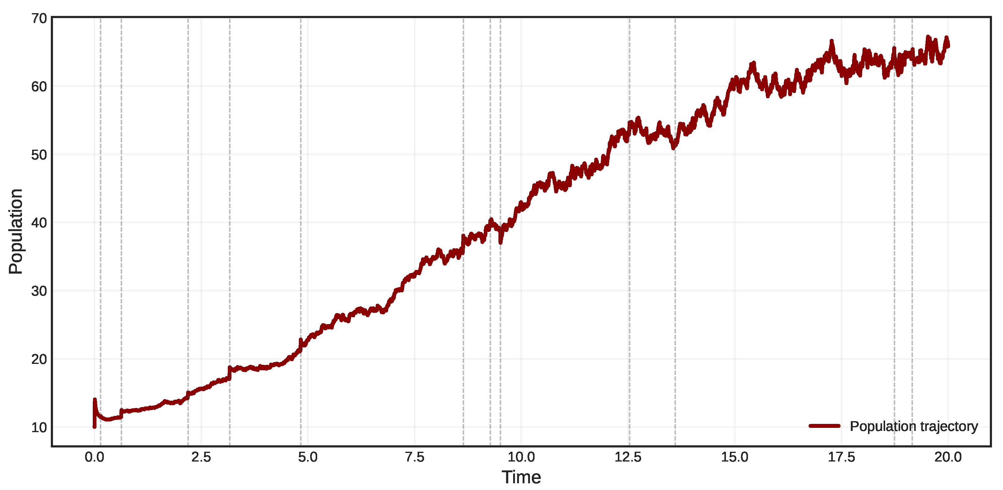
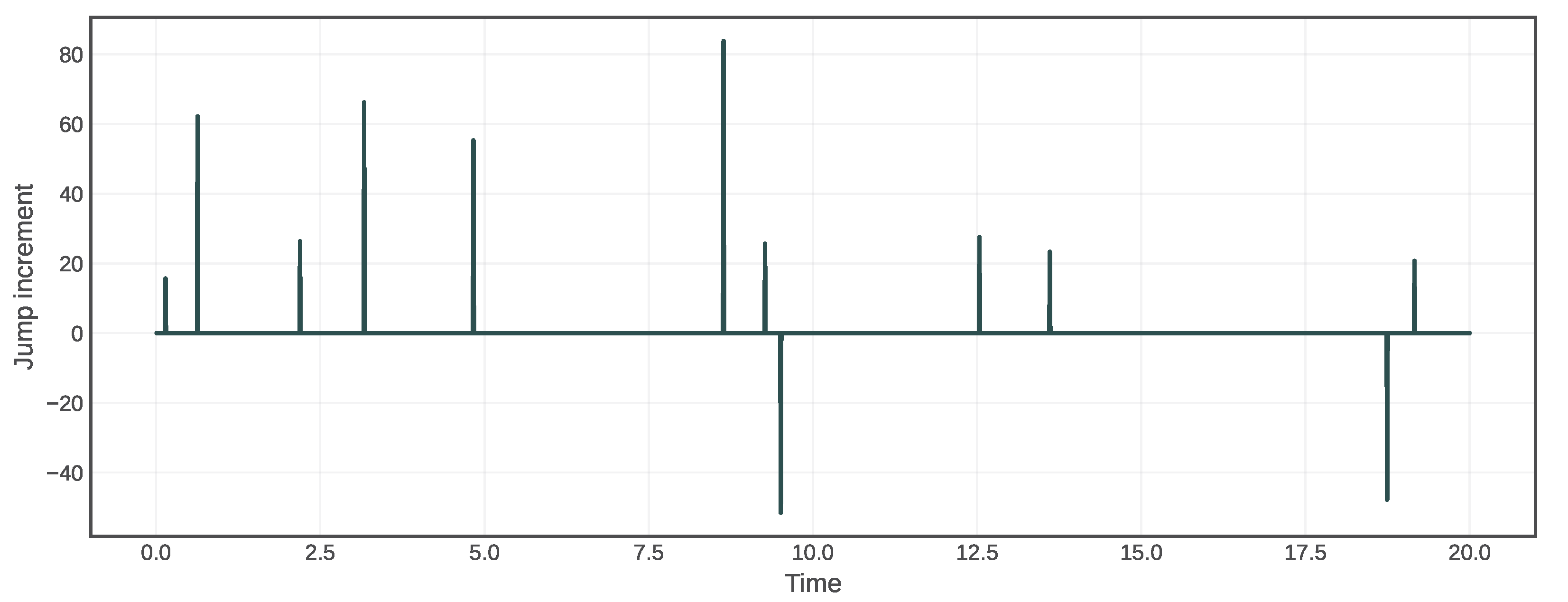
Figure 1 and Figure 2 present numerical simulations of the $\gamma$-Hilfer fractional stochastic population model with delay and Poisson jumps. Figure 1 illustrates a representative trajectory of the population process, while Figure 2 displays the corresponding jump increments generated by the compound Poisson process.

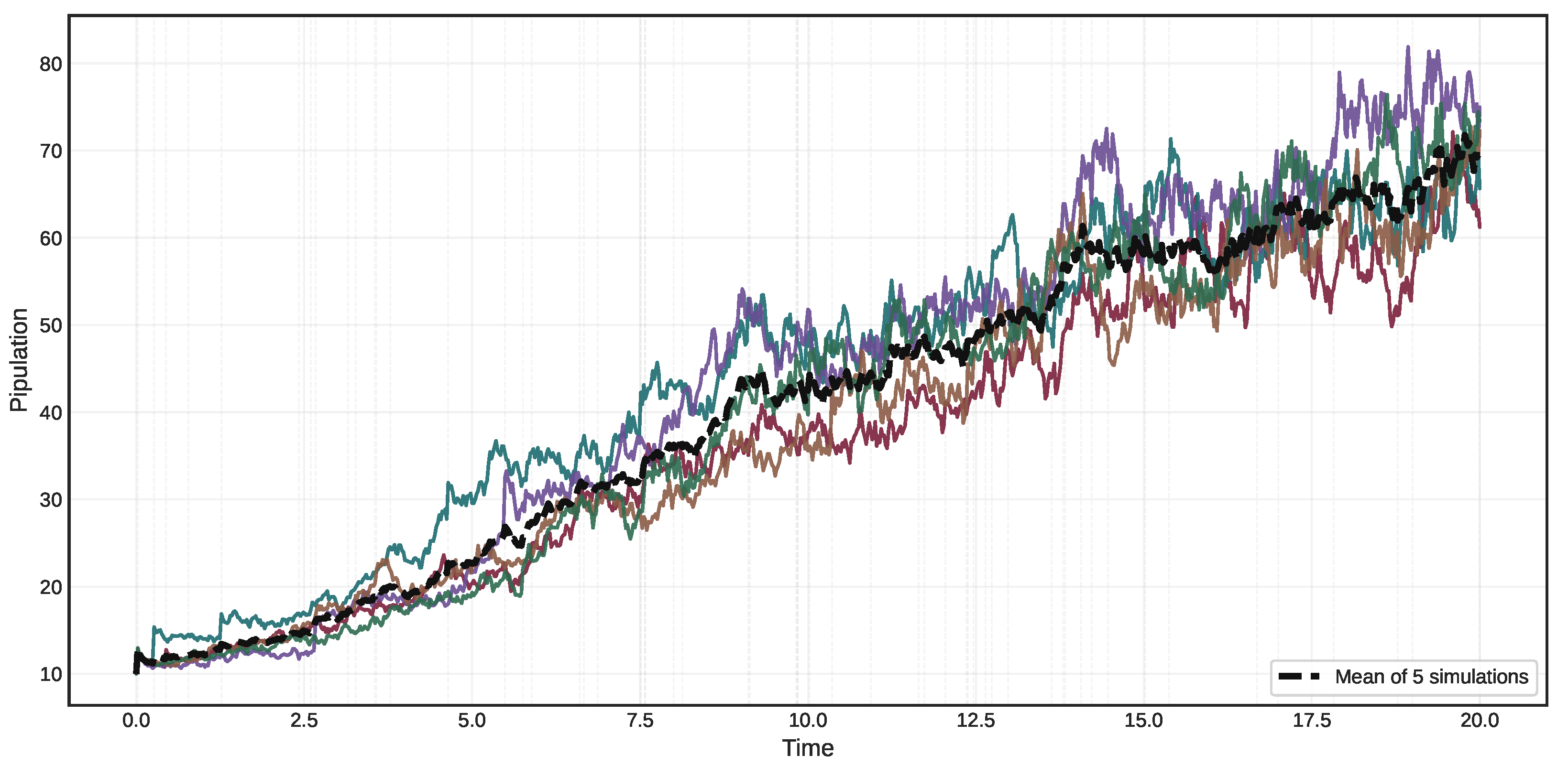
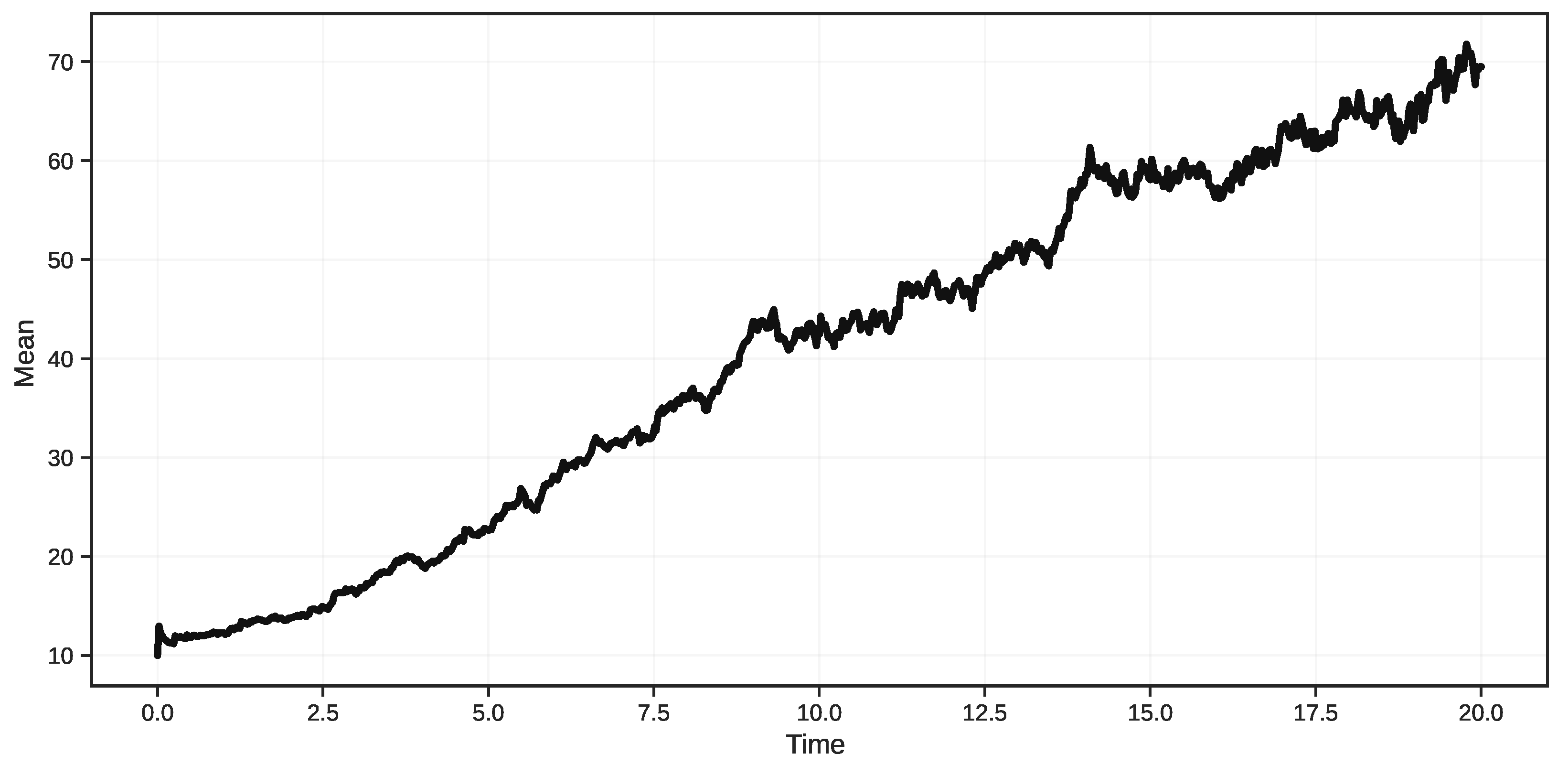
Figure 3 and Figure 4 present numerical simulations of the $\gamma$-Hilfer fractional stochastic population model with delay and Poisson jumps. Figure 3 shows five independent sample paths together with their mean trajectory, illustrating the combined effects of memory, delay, diffusion, and jump disturbances. Figure 4 depicts the corresponding mean evolution of the population process.

6. Conclusions

Our considered system incorporates both Brownian motion and Poisson jumps, making the direct application of the BCP considerably more challenging compared to its use in FSDEs driven solely by standard Brownian motion. Therefore, we employ the BCP within this more complex framework to address the additional jump components effectively. Similarly, establishing the results of the averaging principle for FSDEs involving standard Brownian motion and Poisson jumps is more difficult than for systems influenced only by Brownian motion.

We made significant contributions to establishing the results for both Ex-Un and Av-Pr. First, by deriving results for the p-th moment, we expanded the findings beyond the specific case of $p=2$. Second, we established these results within the context of the $\gamma$-HFrD. Third, we addressed FSDEs driven by both Brownian motion and Poisson jumps, thus covering a wider class of stochastic systems.

7. Future Directions

Future research may focus on extending the present analysis to systems driven by more general noise processes, impulsive effects, distributed delays, or control and optimization problems associated with fractional stochastic delay systems.

References

1. Sharma, N.; Mishra, S.K.; Hamdi, A. Hermite-Hadamard type inequality for ψ-Riemann-Liouville fractional integrals via preinvex functions. Int. J. Nonlinear Anal. Appl. 2022, 13, 3333–3345. [Google Scholar]
2. Awadalla, M.; Noupoue, Y.Y.Y.; Asbeh, K.A.; Ghiloufi, N. Modeling Drug Concentration Level in Blood Using Fractional Differential Equation Based on ψ-Caputo Derivative. J. Math. 2022, 2022, 9006361. [Google Scholar] [CrossRef] [Scilit]
3. Abdelhedi, W. On a piecewise ψ-Hilfer fractional differential equation. Complex Var. Elliptic Equ. 2026, 71, 374–391. [Google Scholar] [CrossRef] [Scilit]
4. Sakthivel, R.; Revathi, P.; Ren, Y. Existence of solutions for nonlinear fractional stochastic differential equations. Nonlinear Anal. Theory Methods Appl. 2013, 81, 70–86. [Google Scholar] [CrossRef] [Scilit]
5. El-Borai, M.M. Some probability densities and fundamental solutions of fractional evolution equations. Chaos Solitons Fractals 2010, 43, 159–167. [Google Scholar] [CrossRef] [Scilit]
6. Zhang, Q. Existence and uniqueness of solutions for fractional stochastic differential equations with delay. Stat. Probab. Lett. 2017, 124, 47–54. [Google Scholar]
7. Yang, M. Existence and uniqueness of mild solutions for G-Caputo fractional stochastic evolution equations with delay driven by fractional Brownian motion. J. Math. Anal. Appl. 2021, 495, 124755. [Google Scholar]
8. Wang, J. Stochastic delay evolution equations driven by fractional Brownian motion. Stoch. Anal. Appl. 2024, 42, 1–23. [Google Scholar]
9. Maheswari, K.; Radhakrishnan, R.; Park, J.H. Existence, uniqueness, and stability of tempered fractional stochastic differential equations with Lévy noise. J. Comput. Appl. Math. 2024, 430, 115174. [Google Scholar]
10. Makhloufa, M.; Hammouch, Z.; Baleanu, D. Hyers–Ulam stability for Hadamard fractional stochastic differential equations. Fractal Fract. 2023, 7, 118. [Google Scholar]
11. Chen, H. Stability analysis of fractional stochastic differential equations. J. Appl. Math. Comput. 2022, 68, 215–232. [Google Scholar]
12. Ahmadova, A.; Allahverdiyev, B.; Zeynally, R. Ulam–Hyers stability of Caputo-type fractional stochastic differential equations. Mathematics 2021, 9, 2684. [Google Scholar] [CrossRef] [Scilit]
13. Luo, D.; Wang, J.; Ren, Y. Averaging principle for fractional stochastic differential equations with time delay. Appl. Math. Comput. 2020, 372, 124993. [Google Scholar] [CrossRef] [Scilit]
14. Ren, Y.; Xiao, Y. Averaging principle for Caputo fractional stochastic differential equations driven by Lévy noise. Stoch. Anal. Appl. 2024, 42, 389–410. [Google Scholar]
15. Jalisraj, A. Averaging principle for Riemann–Liouville fractional stochastic differential equations with delay. Stoch. Dyn. 2025, 25, 2550004. [Google Scholar]
16. Raheem, M.A.; Selvaraj, S.; Baleanu, D. Controllability of G-Hilfer fractional stochastic neutral differential systems. Chaos Solitons Fractals 2024, 176, 114068. [Google Scholar]
17. Hussain, A.; Ahmad, B.; Alsaedi, A. Controllability of Hilfer fractional stochastic differential equations with infinite delay. Adv. Differ. Equ. 2024, 2024, 87. [Google Scholar]
18. Lin, S.J. Stochastic analysis of fractional Brownian motions. Stoch. Int. J. Probab. Stoch. Processes 1995, 55, 121–140. [Google Scholar] [CrossRef] [Scilit]
19. Son, D.T.; Huong, P.T.; Kloeden, P.E.; Tuan, H.T. Asymptotic separation between solutions of Caputo fractional stochastic differential equations. Stoch. Anal. Appl. 2018, 36, 654–664. [Google Scholar] [CrossRef] [Scilit]
Figure 1. Sample trajectory of the γ -Hilfer fractional population model with delay and Poisson jumps; dashed lines mark jump events.
Axioms 15 00305 g001
Figure 2. Compound Poisson jump increments indicating the timing and magnitude of random shocks.
Axioms 15 00305 g002
Figure 3. Five sample paths of the γ -Hilfer fractional population model with their mean trajectory.
Axioms 15 00305 g003
Figure 4. Mean trajectory of the γ -Hilfer fractional stochastic population model over five simulations.
Axioms 15 00305 g004
Disclaimer/Publisher’s Note: The statements, opinions and data contained in all publications are solely those of the individual author(s) and contributor(s) and not of MDPI and/or the editor(s). MDPI and/or the editor(s) disclaim responsibility for any injury to people or property resulting from any ideas, methods, instructions or products referred to in the content.