Upper and Lower Bounds for Eigenvalues of the Elliptic Operator by Weak Galerkin Quadrilateral Spectral Element Methods

Abstract

In this study, we investigate the upper- and lower-bound approximations of numerical eigenvalues derived by weak Galerkin spectral element methods on arbitrary convex quadrilateral meshes for the Laplace eigenvalue problem. Firstly, the Piola transformation is employed to construct the approximation space for weak gradients on each convex quadrilateral element, while a one-to-one mapping is used to establish the approximation space for weak functions. Subsequently, based on the weak Galerkin spectral element approximation space defined on convex quadrilateral meshes, a Galerkin approximation scheme is formulated, and its well-posedness is then analyzed. Furthermore, numerical experiments are performed on arbitrary convex quadrilateral meshes of the square and L-shaped domains to explore the upper- and lower-bound approximations of numerical eigenvalues. Numerical findings indicate that the presented method not only obtains optimal orders of convergence with respect to both the mesh size and the polynomial degree, but also provides upper- and lower-bound approximations for the reference eigenvalues by proper choices of polynomial degrees in approximation spaces and parameters of the approximation scheme in both h-version and p-version weak Galerkin spectral element methods. This study offers new perspectives and methodologies for the high-precision numerical solution of eigenvalue problems in elliptic equations.

1. Introduction

The eigenvalue problems for second-order elliptic equations are a classic type of partial differential equations. They have been widely applied in scientific computing and engineering fields, such as quantum chemistry, elasticity, and vibration analysis. However, the exact solutions of general eigenvalue problems of second-order elliptic equations cannot usually be expressed explicitly. Thus, developing efficient and effective numerical methods for solving such problems is of great practical significance. It is also crucial to further investigate properties of numerical eigenvalues, as this helps reveal the stability and dynamic behaviors of the corresponding systems.

The commonly used numerical methods are finite difference, finite element, spectral and spectral element methods. Indeed, eigenvalue problems are naturally global problems. Spectral and spectral element methods adopt infinitely smooth, high-order orthogonal polynomials, such as trigonometric polynomials, Jacobi polynomials, Chebyshev polynomials, and Legendre polynomials. These polynomials are used to construct trial function spaces and test function spaces, which easily yields equivalent algebraic eigenvalue systems with sparse matrices and favorable condition numbers. Therefore, compared with the finite element and finite difference methods, global spectral and spectral element methods are more suitable for numerically solving eigenvalue problems.

The weak Galerkin finite element method is a recently developed nonconforming finite element method, initially introduced to solve second-order elliptic equations [1]. Its key principle lies in approximating unknown solutions by weak functions with interior and boundary parts, and in approximating classical differential operators via discrete weak operators on weak function spaces. This method applies to arbitrary meshes consisting of arbitrary polygons or polyhedra [2]. It further allows diverse choices of polynomial degrees in the approximation spaces for weak gradients and weak functions [3], thus featuring considerable flexibility and robustness. By virtue of these merits, the method has been widely studied for second-order elliptic equations [4,5,6,7]. In particular, for eigenvalue problems, it achieves asymptotic lower-bound approximations by linear finite elements [8], in contrast to the existing nonconforming finite element methods. It also yields high-quality approximations to exact eigenvalues from below or above by adjusting the global penalty parameter within its approximation framework [9]. Therein, a high-accuracy algorithm for eigenvalue computation is designed to achieve a higher convergence order at a lower cost. In [10], this method is employed to derive lower bounds of Laplacian eigenvalues, while a post-processing technique is adopted to obtain upper bounds. Furthermore, this method has been applied to diverse problems like Burgers equation [11], Stokes equation [12,13], the Maxwell problem [14], and parabolic singularly perturbed convection–diffusion equations [15].

Combining the flexibility of the weak Galerkin finite element method with the high-order accuracy of the spectral element method, a nonconforming weak Galerkin spectral element method is introduced for eigenvalue problems [16]. In contrast to the weak Galerkin finite element method, this new method defines two key approximation spaces. The space for weak functions on triangles or parallelograms is constructed by one-to-one mappings from orthogonal polynomials defined on the reference element, and that for weak gradients by the Piola transformation. Error estimates are proven to be optimal in the mesh size and suboptimal in the polynomial degree. Furthermore, in [17], another type of one-to-one mapping is used to construct the approximation space for weak gradients, while the super-convergence and the lower-bound approximation are explored with various choices of polynomial degrees. Subsequently, a modified weak Galerkin spectral element method [18] is presented for obtaining the optimal $hp$ error estimates with respect to the mesh size and the polynomial degree. Thus, the weak Galerkin spectral element method not only offers a novel way to investigate eigenvalue problems, it also broadens the applicability of weak Galerkin methods and spectral element methods.

In summary, there are two novel contributions in the present work: one is the systematic investigation of upper- and lower-bound approximations of eigenvalues based on the approximation space of weak gradients constructed via the Piola transformation. This construction approach differs from that in [17], especially on quadrilateral meshes; the other is a further study of upper- and lower-bound approximations of eigenvalues under various polynomial combinations on arbitrary quadrilateral meshes, in contrast to the convergence study in [16], which is conducted under a specific polynomial combination on triangular/parallelogram meshes. Indeed, compared to triangular/parallelogram elements, non-parallelogram quadrilateral elements are technically nontrivial. First, the mapping from a reference square to a general quadrilateral element is bilinear, rather than affine. The corresponding Jacobian matrix is not constant, which renders the integrands for mass and stiffness matrices more complex and necessitates more sophisticated integration strategies. Moreover, when a quadrilateral deviates from a standard rectangle, the bilinear mapping compromises the strict separability of the tensor product basis, increasing the complexity of algorithm implementation. In particular, if quadrilateral elements are severely distorted, the bilinear mapping can cause dramatic variations in the Jacobian determinant, adversely affecting computational accuracy and stability. Nevertheless, quadrilateral meshes still retain the inherent potential for computational efficiency offered by the tensor product structure. Therefore, generating high-quality quadrilateral meshes is a significant technical challenge, and systematically investigating the properties of weak Galerkin spectral element methods for solving eigenvalue problems on such meshes is essential to extend their application to practical scientific and engineering problems.

In addition, several eigenvalue approximation methods also provide guaranteed eigenvalue bounds. For example, guaranteed and optimally convergent a posteriori bounds for both an arbitrary separated Laplace eigenvalue and the associated eigenvector are obtained by the conforming finite element method [19]. Beyond conforming methods, a skeletal finite element method with an appropriate stabilization is proposed in [20] to deliver guaranteed lower eigenvalue bounds for the Laplacian on triangular meshes. Furthermore, an extra-stabilized nonconforming Crouzeix–Raviart finite element eigensolver is introduced on triangulation [21]. It provides guaranteed lower Dirichlet eigenvalue bounds and achieves optimal convergence rates of the guaranteed lower bounds towards simple eigenvalues. Additionally, a unified derivation of three skeletal higher-order methods is presented in [22], which suggests a paradigm shift from conditional to unconditional lower eigenvalue bounds. Compared to these methods, our method reveals more upper- and lower-bound approximation scenarios of eigenvalues on arbitrary quadrilateral meshes, which can be obtained by matching polynomial degrees in approximation spaces and the parameter in the stabilizer. More importantly, in contrast to these h-version methods, our $hp$-version method enables us to obtain upper and lower bounds of eigenvalues in the framework of p-version weak Galerkin spectral element method. Finally, it should be noted that the upper- and lower-bound approximations of eigenvalues presented in this paper are currently validated numerically rather than rigorously proved.

This paper aims to study the upper- and lower-bound approximations of numerical eigenvalues obtained by weak Galerkin spectral element methods for the Laplacian eigenvalue problem on arbitrary convex quadrilateral meshes. On each convex quadrilateral element, the approximation space for weak gradients is constructed from orthogonal polynomials on the reference square through the Piola transformation. We then construct the approximation spaces with various choices of polynomial degrees and establish the well-posed approximation scheme on arbitrary convex quadrilateral meshes. Next, we focus on the investigation of the upper- and lower-bound approximations of numerical eigenvalues on quadrilateral meshes of the square and L-shaped domains. Numerical experiments demonstrate that such upper- and lower-bound approximations can be achieved in both the h- and p-version methods by suitable choices of polynomial degrees in the approximation spaces for weak gradients and weak functions, as well as suitable choices of parameters in the approximation scheme.

This paper is structured in the following manner. Section 2 introduces commonly used notations and definitions of weak functions and weak gradients, along with their discrete forms. In Section 3, the weak Galerkin spectral element approximation space and the approximation scheme are constructed. In Section 4, the upper- and lower-bound approximations of numerical eigenvalues are explored on the square and L-shaped domains. Finally, Section 5 concludes this work and further discusses directions for future research.

2. Weak Gradients and Spectral Weak Gradients

This section first introduces commonly used notations. The set of non-negative integers is represented by ${\mathbb{N}}_0$, and the reference square is defined as $\widehat{Q}={(-1,1)}^2$. For any $n\in {\mathbb{N}}_0$, denote by ${\mathbb{Q}}_n\left(\widehat{Q}\right)$ the space of polynomials on $\widehat{Q}$ with degree ≤$n$ in each variable. The mapped polynomial space ${\mathbb{Q}}_n\left(Q\right)$ on a general convex quadrilateral Q can be defined as

$${\mathbb{Q}}_n\left(Q\right):=\{v=\widehat{v}\circ {\mathsf{\Phi }}_Q^{-1}:\forall \widehat{v}\in {\mathbb{Q}}_n\left(\widehat{Q}\right)\},$$

where ${\mathsf{\Phi }}_Q:\widehat{Q}\mapsto Q$ is a one-to-one mapping [16]. Moreover, for any $m\in {\mathbb{N}}_0$, denote by $X_m(\partial Q)$ the piecewise polynomial space with degree ≤$m$ on the boundary $\partial Q$, i.e.,

$$X_m(\partial Q):=\{v:v\in {\mathbb{Q}}_m\left(e\right)\mathrm{for}\mathrm{each}\mathrm{edge}e\mathrm{of}Q\}.$$

2.1. Weak Functions and Weak Gradients

A weak function defined on Q is denoted by $v=\{v_0,v_b\}$, with $v_0\in L^2\left(Q\right)$ and $v_b\in L^2(\partial Q)$. Note that $v_0$ and $v_b$ correspond to the values of v in the interior of Q and on its boundary $\partial Q$, respectively. The space of all weak functions on Q is denoted by $W\left(Q\right)$, i.e.,

$$W\left(Q\right)=\left\{v=\{v_0,v_b\}:v_0\in L^2\left(Q\right),v_b\in L^2(\partial Q)\right\}.$$

It is clear that for any $f\in H^s\left(Q\right)$ with $s\ge {\displaystyle \frac{1}{2}}$, $f\in W\left(Q\right)$ is equivalent to $\{f,f{|}_{\partial Q}\}\in W\left(Q\right)$.

Definition 1

([1,4]). For any $v\in W\left(Q\right)$, its weak gradient ${\nabla }_{w}v$ is defined to be the unique linear functional in ${\left[H^1{\left(Q\right)}^2\right]}^{\prime }$ satisfying

$$\begin{array}{c}\hfill {({\nabla }_{w}v,\mathit{q})}_Q:=-{(v_0,\nabla ·\mathit{q})}_Q+{(v_b,\mathit{q}·\mathbf{n})}_{\partial Q},\forall \mathit{q}\in H^1{\left(Q\right)}^2,\end{array}$$

where ∇ is the classical gradient operator in the general coordinates $(x,y)$, and $\mathbf{n}$ is the outward normal direction to $\partial Q$.

2.2. Spectral Weak Gradients

For practical computation, we introduce the following definition of discrete weak gradients on a convex quadrilateral element.

Definition 2

([23]). Let ${\mathcal{Q}}_N\left(Q\right)\subset H^1{\left(Q\right)}^2$ be a finite-dimensional space. For any $v\in W\left(Q\right)$, its discrete weak gradient is specified as the unique ${\nabla }_{N}v\in {\mathcal{Q}}_N\left(Q\right)$ satisfying

$$\begin{array}{c}\hfill {({\nabla }_{N}v,\mathit{q})}_Q:=-{(v_0,\nabla ·\mathit{q})}_Q+{(v_b,\mathit{q}·\mathbf{n})}_{\partial Q},\forall \mathit{q}\in {\mathcal{Q}}_N\left(Q\right).\end{array}$$

(1)

If we assume that $v_0\in H^1\left(K\right)$, then applying the Green’s formula to (1) yields

$$\begin{array}{c}\hfill {({\nabla }_{N}v,\mathit{q})}_Q={(\nabla v_0,\mathit{q})}_Q+{(v_b-v_0,\mathit{q}·\mathbf{n})}_{\partial Q},\forall \mathit{q}\in {\mathcal{Q}}_Q\left(Q\right).\end{array}$$

In this paper, we construct the weak gradient approximation space via the Piola transformation [24] to obtain higher-order approximation,

$$\begin{array}{c}\hfill {\mathcal{Q}}_N\left(Q\right)=\left\{\mathit{q}=\left[J_Q^{-1}{F}_Q\widehat{\mathit{q}}\right]\circ {\mathsf{\Phi }}_Q^{-1}:\forall \widehat{\mathit{q}}\in {\mathbb{Q}}_N{\left(\widehat{Q}\right)}^2\right\},\end{array}$$

(2)

in which $F_Q$ and $J_Q$ denote the Jacobian matrix of the mapping ${\mathsf{\Phi }}_Q$ and the corresponding determinant, respectively.

There are some remarkable properties of the Piola transformation [24] Lemma 3.59, i.e., for any $\mathit{q}=\left[J_Q^{-1}{F}_Q\widehat{\mathit{q}}\right]\circ {\mathsf{\Phi }}_Q^{-1}\in {\mathcal{Q}}_N\left(Q\right)$, it holds that

$$\begin{array}{c}\hfill \begin{array}{c}\hfill \nabla ·\mathit{q}=J_K^{-1}\widehat{\nabla }·\widehat{\mathit{q}},{(w,\nabla ·\mathit{q})}_Q={(\widehat{w},\widehat{\nabla }·\widehat{\mathit{q}})}_{\widehat{Q}},\widehat{\mathit{q}}\in {\mathbb{Q}}_N{\left(\widehat{Q}\right)}^2,\end{array}\end{array}$$

(3)

where $w=\widehat{w}\circ {\mathsf{\Phi }}_Q^{-1}$ and $\widehat{\nabla }$ denotes the classical gradient operator in the reference coordinates $(\widehat{x},\widehat{y})$. Thus, it is easy to obtain that $\nabla ·\mathit{q}=0$ if and only if $\widehat{\nabla }·\widehat{\mathit{q}}=0$.

Hence, combining (1), (3) with [23], we have

$$\begin{array}{c}\hfill {({\nabla }_{N}v,\mathit{q})}_Q=-{({\widehat{v}}_0,\widehat{\nabla }·\widehat{\mathit{q}})}_{\widehat{Q}}+{({\widehat{v}}_b,\widehat{\mathit{q}}·\widehat{\mathit{n}})}_{\partial \widehat{Q}}={({\widehat{\nabla }}_N\widehat{v},\widehat{\mathit{q}})}_{\widehat{Q}},\end{array}$$

(4)

where ${\widehat{v}}_0=v_0\circ {\mathsf{\Phi }}_Q$, ${\widehat{v}}_b=v_b\circ {\mathsf{\Phi }}_Q{|}_{\partial \widehat{Q}}$, $\widehat{\mathbf{n}}$ is the outward normal direction to the boundary $\partial \widehat{Q}$, and ${\widehat{\nabla }}_N$ is the discrete weak gradient operator on $\widehat{Q}$. By (4), the inner product of the discrete weak gradient on a general quadrilateral element can be transformed into the corresponding inner product on the reference square, thereby simplifying and unifying the computation.

Further details on discrete weak gradients are available in [16,23].

Next, we define the approximation space, denoted by $W_{n,m}\left(Q\right)$, for weak functions on a convex quadrilateral element Q, i.e.,

$$\begin{array}{c}\hfill W_{n,m}\left(Q\right)=\{v=\{v_0,v_b\}:v_0\in {\mathbb{Q}}_n\left(Q\right),v_b\in X_m(\partial Q)\}.\end{array}$$

(5)

Given the approximation spaces for weak gradients and weak functions defined in (2) and (5), the discrete weak gradient ${\nabla }_{N}v$ for any $v\in W_{n,m}\left(Q\right)$ can be referred to as the spectral weak gradient.

3. Weak Galerkin Spectral Element Method

In this section, we focus on developing a weak Galerkin spectral element approximation for the eigenvalue problem of elliptic operators.

3.1. Model Problem

Let us consider the following model problem,

$$\left\{\begin{array}{c}\begin{array}{cccc}\hfill -\Delta u& =\lambda u,\hfill & \hfill & \mathrm{in}\mathsf{\Omega },\hfill \\ \hfill u& =0,\hfill & \hfill & \mathrm{on}\partial \mathsf{\Omega },\hfill \end{array}\hfill \end{array}\right.$$

(6)

where $\mathsf{\Omega }\subset {\mathbb{R}}^2$ is a polygonal domain, $\lambda$ is the exact eigenvalue, and u is the corresponding eigenfunction.

For the eigenvalue problem (6), the classical variational formulation is to find $\lambda \in \mathbb{R}$ and $u\in H_0^1\left(\mathsf{\Omega }\right)$ with $b(u,u)=1$ satisfying

$$\begin{array}{c}\hfill a(u,v)=\lambda b(u,v),\forall v\in H_0^1\left(\mathsf{\Omega }\right),\end{array}$$

where $a(u,v):=(\nabla u,\nabla v)$ and $b(u,v):=(u,v)$. From the result presented in [25], the Rayleigh quotient is defined as

$$\begin{array}{c}\hfill R\left(u\right):={\displaystyle \frac{a(u,u)}{b(u,u)}}=\lambda .\end{array}$$

3.2. Weak Galerkin Spectral Element Approximation

To construct the approximation scheme for the problem (6), we first partition the computational domain $\mathsf{\Omega }$ into convex quadrilateral elements and denote by ${\mathcal{T}}_h=\left\{Q_i\right\}$ the partition of $\mathsf{\Omega }$. For simplicity, the partition ${\mathcal{T}}_h$ is presumed to be conforming and shape-regular, i.e.,

$$\begin{array}{c}\hfill \parallel F_Q(\widehat{x},\widehat{y})\parallel \parallel F_Q^{-1}(\widehat{x},\widehat{y})\parallel \le C,\forall Q\in {\mathcal{T}}_h,(\widehat{x},\widehat{y})\in \widehat{Q},\end{array}$$

in which C denotes a positive constant independent of any discretization parameters and functions. Let ${\mathcal{E}}_h^0$ denote the set of all interior edges of the partition ${\mathcal{T}}_h$.

For any $n,m\in {\mathbb{N}}_0$, we define the weak Galerkin spectral element approximation space on ${\mathcal{T}}_h$,

$$\begin{array}{cc}\hfill & W_{\delta }:=\left\{w=\{w_0,w_b\}:w_0{{|}_Q\in {\mathbb{Q}}_n\left(Q\right),\forall Q\in {\mathcal{T}}_h;w_b|}_e\in {\mathbb{Q}}_m\left(e\right),\forall e\in {\mathcal{E}}_h^0\right\},\hfill \\ \hfill & W_{\delta }^0:=\left\{w\in W_{\delta }:w_b{|}_e=0,\forall e\in \partial Q\cap \partial \mathsf{\Omega },\forall Q\in {\mathcal{T}}_h\right\},\hfill \end{array}$$

where $\delta =\delta (h,n,m,N)$ represents a discretization parameter dependent on the mesh size and the polynomial degrees.

For any $w,v\in W_{\delta }^0$, we define the bilinear form $a_{\delta }$ by

$$\begin{array}{c}\hfill a_{\delta }(w,v):=\sum _{K\in {\mathcal{T}}_h}{({\nabla }_{N}w,{\nabla }_{N}v)}_K+s(w,v),\end{array}$$

(7)

where the stabilizer $s(w,v)$ is given by

$$s(w,v):=\rho \sum _{K\in {\mathcal{T}}_h}{h}_K^{-1}{N}^2{(w_0-w_b,v_0-v_b)}_{\partial K},\rho \ge 0.$$

Then, the weak Galerkin spectral element approximation scheme for the model problem (6) is to find ${\lambda }_{\delta }\in \mathbb{R}$ and $u_{\delta }=\{u_{\delta ,0},u_{\delta ,b}\}\in W_{\delta }^0$ with $u_{\delta }\ne 0$ and $b_{\delta }(u_{\delta },u_{\delta })=1$ such that

$$\begin{array}{c}\hfill a_{\delta }(u_{\delta },v)={\lambda }_{\delta }{b}_{\delta }(u_{\delta },v),\forall v\in W_{\delta }^0,\end{array}$$

(8)

where $b_{\delta }(u_{\delta },v):={\sum }_{K\in {\mathcal{T}}_h}{(u_{\delta ,0},v_0)}_K.$

By expanding the approximate solution $u_{\delta }$ in appropriate basis functions and substituting it into (8), we can obtain an equivalent algebraic system. To ensure the solvability of the derived algebraic system, it is necessary to analyze the well-posedness of the proposed scheme (8).

Theorem 1 

([23]). The bilinear form (7) is positive definite if either of the following conditions is satisfied:

(i) 

$n\le N$ and $m\in {\mathbb{N}}_0$ for $\rho >0$;

(ii) 

$n\le N-1$ and $m\le N$ for $\rho =0$.

From Theorem 1, we obtain that $a_{\delta }(w,w)=0$ with $w\in W_{\delta }^0$ implies $w_0=0$ in $\mathsf{\Omega }$ and $w_b=0$ on all edges of ${\mathcal{T}}_h$. Then, we introduce the following norm in $W_{\delta }^0$,

$${\parallel w\parallel }_{W_{\delta }^0}^2=\sum _{K\in {\mathcal{T}}_h}\left(\parallel {\nabla }_N{w\parallel }_K^2+\rho h_K^{-1}{N}^2{\parallel w_0-w_b\parallel }_{\partial K}^2\right),\forall w\in W_{\delta }^0.$$

(9)

It is easy to verify that the bilinear form $a_{\delta }(w,v)$ is symmetric, i.e.,

$$a_{\delta }(w,v)=a_{\delta }(v,w),\forall w,v\in W_{\delta }^0.$$

(10)

In addition, we can derive from (7), the triangle inequality, (9), and the Cauchy–Schwarz inequality that the bilinear form is continuous, i.e.,

$$|a_{\delta }(w,v)|\le C{\parallel w\parallel }_{W_{\delta }^0}{\parallel v\parallel }_{W_{\delta }^0},\forall w,v\in W_{\delta }^0,$$

(11)

where $C>0$ is a constant. Furthermore, from (7) and (9), we directly obtain

$$a_{\delta }(w,w)={\parallel w\parallel }_{W_{\delta }^0}^2,\forall w\in W_{\delta }^0.$$

(12)

This identity immediately implies that the bilinear form $a_{\delta }(·,·)$ is coercive on $W_{\delta }^0$ with a coercivity constant of 1.

Therefore, the approximation scheme (8) is well-posed. The positive definiteness and the coercivity, together with the symmetry of the bilinear form, guarantee that all approximate eigenvalues are real and positive. Thus, no zero eigenvalues or spurious eigenvalues would arise in numerical computations.

In addition, for the eigenvalue ${\lambda }_{\delta }$ and its corresponding eigenfunction $u_{\delta }$, the following Rayleigh quotient holds,

$$\begin{array}{c}\hfill R\left(u_{\delta }\right):={\displaystyle \frac{a_{\delta }(u_{\delta },u_{\delta })}{b_{\delta }(u_{\delta },u_{\delta })}}={\lambda }_{\delta }.\end{array}$$

Let ${\lambda }_i,i\in \mathbb{N}$, be the i-th exact eigenvalue and ${\lambda }_{i,\delta },i\in \mathbb{N}$, be the i-th numerical eigenvalue, respectively, where $\mathbb{N}$ denotes the set of positive integers. These eigenvalues are ordered as,

$${\lambda }_1<{\lambda }_2\le {\lambda }_3\le \cdots \le {\lambda }_i\le {\lambda }_{i+1}\le \dots ,$$

$${\lambda }_{1,\delta }<{\lambda }_{2,\delta }\le {\lambda }_{3,\delta }\le \cdots \le {\lambda }_{i,\delta }\le {\lambda }_{i+1,\delta }\le \dots .$$

Then due to the symmetry and coercivity of bilinear forms, the following min–max principle holds for both ${\lambda }_i$ and ${\lambda }_{i,\delta }$ [25,26]:

$$\begin{array}{cc}\hfill & {\lambda }_i=\underset{\begin{array}{c}{V}_i\subset H_0^1\left(\mathsf{\Omega }\right)\\ dim{V}_i=i\end{array}}{min}\underset{w\in V_i}{max}R\left(w\right),\hfill \\ & {\lambda }_{i,\delta }=\underset{\begin{array}{c}{V}_{i,\delta }\subset W_{\delta }^0\\ dim{V}_{i,\delta }=i\end{array}}{min}\underset{w_{\delta }\in V_{i,\delta }}{max}R\left(w_{\delta }\right),\hfill \end{array}$$

which provides a theoretical foundation for deriving upper- and lower-bound approximations of eigenvalues using the weak Galerkin spectral element method.

Based on the approximation space (2) for weak gradients, the computational accuracy of the approximation scheme (8) subject to constraints of Theorem 1 has been validated in [23]. In the following section, we further explore the upper- and lower-bound approximations of numerical eigenvalues in both the h- and p-version methods.

4. Upper- and Lower-Bound Approximations

In this section, we investigate the upper- and lower-bound approximations of numerical eigenvalues obtained by the weak Galerkin spectral element method under the constraints of Theorem 1 for the problem (6) on arbitrary convex quadrilateral meshes of $\mathsf{\Omega }$.

4.1. Qualitative Analysis

We first analyze qualitatively the errors of numerical eigenvalues. In analogy to [17], it can be found that, for any $v=(v_0,v_b)\in W_{\delta }^0$ with any admissible triplets $(n,m,N)$,

$$\begin{array}{cc}\hfill \lambda -{\lambda }_{\delta }& =\sum _{K\in {\mathcal{T}}_h}{\parallel \nabla u-{\nabla }_N{u}_{\delta }\parallel }_K^2+s(u_{\delta }-v,u_{\delta }-v)+2\sum _{K\in {\mathcal{T}}_h}{(\nabla u-{\nabla }_{N}v,{\nabla }_N{u}_{\delta })}_K\hfill \\ & -{\lambda }_{\delta }\sum _{K\in {\mathcal{T}}_h}{\parallel u_{\delta ,0}-v_0\parallel }_K^2-{\lambda }_{\delta }\sum _{K\in {\mathcal{T}}_h}\left(\parallel u_{\delta ,0}{\parallel }_K^2-{\parallel v_0\parallel }_K^2\right)-s(v,v)\hfill \\ & :=I_1+I_2+I_3-{\lambda }_{\delta }{I}_4-{\lambda }_{\delta }{I}_5-I_6,\hfill \end{array}$$

(13)

where $(\lambda ,u)\in {\mathbb{R}}^{+}\times H_0^1\left(\mathsf{\Omega }\right)$ is a normalized exact eigen-pair, and $\left({\lambda }_{\delta },u_{\delta }\right)\in {\mathbb{R}}^{+}\times W_{\delta }^0$ is its approximation eigen-pair.

Therefore, by appropriately matching the polynomial degrees $n,m,N$ subject to the constraints in Theorem 1 and the stabilization parameter $\rho$, either the first two terms or the sixth term dominates in (13), leading to lower- or upper-bound approximation of the eigenvalues, respectively.

As illustrative examples, the square domain $\mathsf{\Omega }={[0,1]}^2$ and the L-shaped domain $\mathsf{\Omega }={[-1,1]}^2{\setminus [0,1]}^2$ are adopted in the following numerical experiments.

4.2. Numerical Study on Square Domain

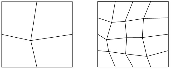
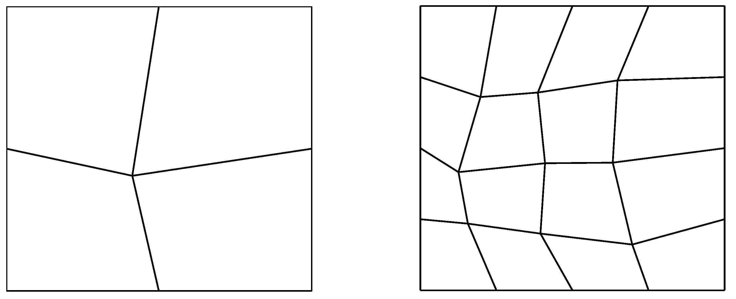
We perform the weak Galerkin spectral element method for the problem (6) on quadrilateral meshes of $\mathsf{\Omega }={[0,1]}^2$ and explore the upper- and lower-bound approximations of numerical eigenvalues. Figure 1 illustrates the computational domain $\mathsf{\Omega }={[0,1]}^2$ as well as the quadrilateral meshes with mesh sizes $h=0.917$ and $h=0.475$.

Figure 1. Computational domain $\mathsf{\Omega }={[0,1]}^2$ and quadrilateral meshes with mesh sizes $h=0.917$ (left) and $h=0.475$ (right).

According to Theorem 1, the approximation scheme (8) is well-posed if $n\le N$ and $m\in {\mathbb{N}}_0$ for $\rho >0$; or if $n\le N-1$ and $m\le N$ for $\rho =0$. Therefore, we discuss the cases of $\rho >0$ and $\rho =0$ separately below.

4.2.1. In the Case of $\rho >0$

We investigate the upper- and lower-bound approximations of numerical eigenvalues on convex quadrilateral meshes of $\mathsf{\Omega }={[0,1]}^2$ in the case of $\rho >0$.

Indeed, the numerical eigenvalues are the lower bounds of the reference eigenvalues in both the h-version and p-version methods

• If $n=N$ and $m\ge N$ for a proper $\rho >0$, such as $\rho \le 0.01$.

In addition, the numerical eigenvalues are the upper bounds of the reference eigenvalues in both the h-version and p-version methods

• If $n=N$ and $m\ge N$ for a proper $\rho >0$, such as $\rho \ge 1$.

In the sequel, we select appropriate values of $\rho$, n, m to investigate numerically.

Let us first take $\rho =0.01$, $n=N$, and $m=N$. As the polynomial degree increases, Table 1 presents the corresponding errors ${\lambda }_i-{\lambda }_{i,\delta },i=1,2,\dots ,5$ with respect to the polynomial degree for $h=0.921$. As observed in Table 1, all the errors are positive. Since the eigenfunctions of the problem (6) are analytic on the square domain, the exponential convergence from below of ${\lambda }_{i,\delta }$ to ${\lambda }_i$ is achieved as the polynomial degree increases.

Table 1. Errors ${\lambda }_i-{\lambda }_{i,\delta }$ ($i=1,2,\dots ,5$) vs. N for $\rho =0.01$, $n=N$, $m=N$ on the quadrilateral mesh with $h=0.921$ of $\mathsf{\Omega }={[0,1]}^2$.

N	${\mathit{\lambda }}_1-{\mathit{\lambda }}_{1,\mathit{\delta }}$	${\mathit{\lambda }}_2-{\mathit{\lambda }}_{2,\mathit{\delta }}$	${\mathit{\lambda }}_3-{\mathit{\lambda }}_{3,\mathit{\delta }}$	${\mathit{\lambda }}_4-{\mathit{\lambda }}_{4,\mathit{\delta }}$	${\mathit{\lambda }}_5-{\mathit{\lambda }}_{5,\mathit{\delta }}$
4	0.043	29.58	29.24	56.87	68.14
5	1.040 × 10−6	19.58	19.01	36.91	50.53
6	1.214 × 10−8	4.889	4.040	29.61	49.35
7	6.160 × 10−12	1.265 × 10−7	9.112 × 10−7	14.35	32.88
8	7.105 × 10−14	2.812 × 10−8	2.198 × 10−8	2.202 × 10−7	7.717
9	1.172 × 10−13	8.730 × 10−11	6.997 × 10−11	9.885 × 10−10	2.914 × 10−6
10	2.878 × 10−13	1.741 × 10−12	1.144 × 10−12	1.259 × 10−11	3.364 × 10−9
11	5.009 × 10−13	3.624 × 10−13	4.974 × 10−14	2.416 × 10−13	3.463 × 10−10

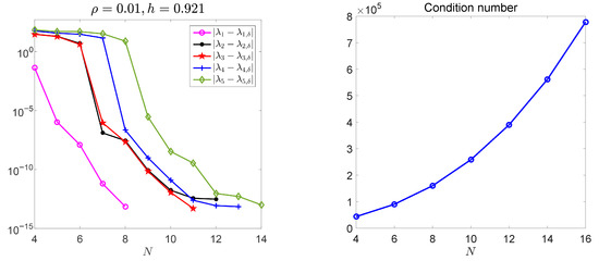
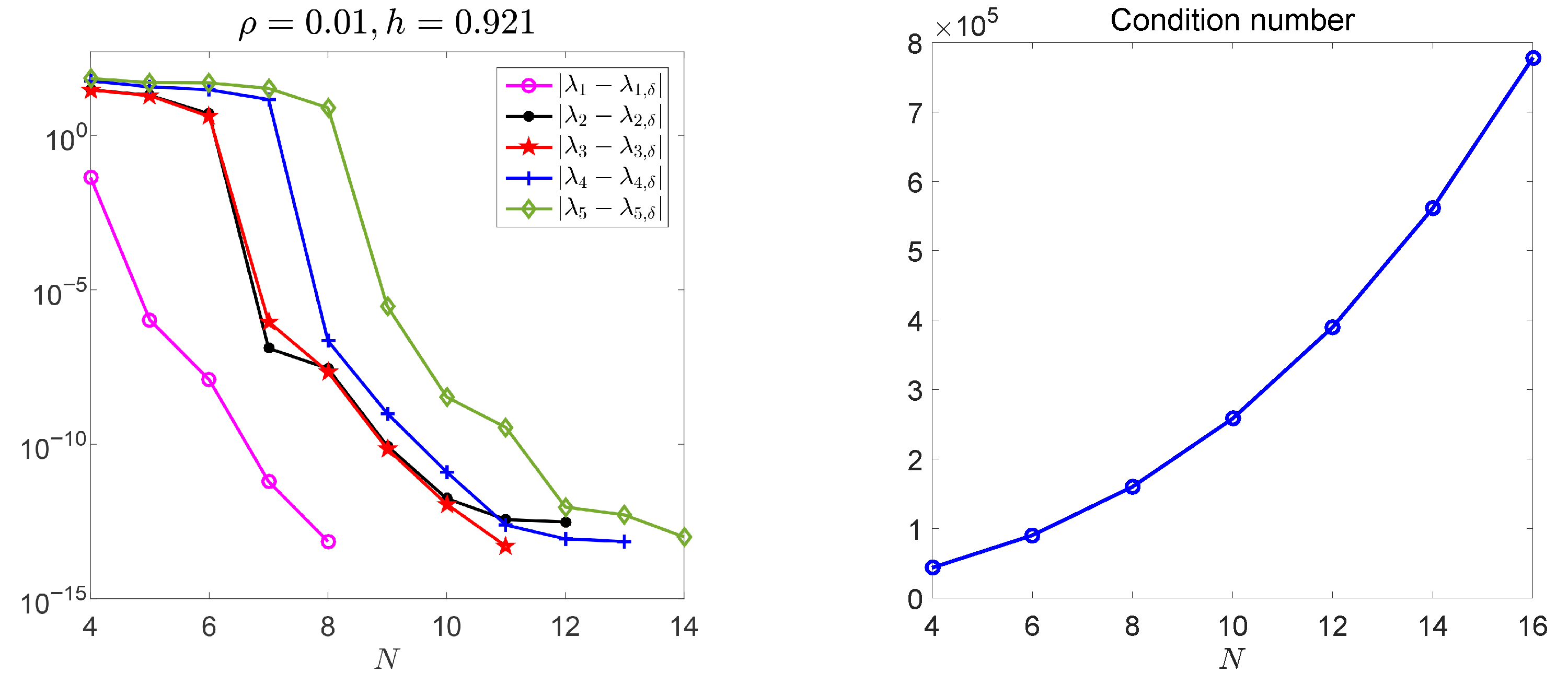
To more clearly illustrate the convergence behaviors of numerical eigenvalues, we also plot the absolute errors $|{\lambda }_i-{\lambda }_{i,\delta }|,i=1,2,\dots ,5$ versus N in semi-log scale for $h=0.921$ in the left panel of Figure 2, which reveals the exponential orders of convergence of the first five numerical eigenvalues with respect to the polynomial degree.

Figure 2. Errors $|{\lambda }_i-{\lambda }_{i,\delta }|,i=1,2,\dots ,5$ vs. N (left) and condition number of stiffness matrix vs. N (right) for $\rho =0.01$, $n=N$, $m=N$ on the quadrilateral mesh of $\mathsf{\Omega }={[0,1]}^2$.

In addition, we plot the condition number of the stiffness matrix versus N for $h=0.818$ in the right panel of Figure 2. As expected, the condition number grows with increasing N. Despite larger condition numbers at higher polynomial degrees, the errors of numerical eigenvalues retain spectral accuracy. This further confirms the effectiveness of our p-version weak Galerkin spectral element method.

Furthermore, the corresponding errors ${\lambda }_i-{\lambda }_{i,\delta },i=1,2,\dots ,5$, and convergence rates with respect to the mesh size for $N=1$ and $N=2$ obtained by the h-version weak Galerkin spectral element method are presented in Table 2. All the errors are positive, which indicates that the numerical eigenvalues are the lower bounds of the exact ones. In addition, the errors converge at rates of approximately $\mathcal{O}\left(h^2\right)$ and $\mathcal{O}\left(h^4\right)$ for $N=1$ and $N=2$, respectively, thereby confirming the lower-bound approximations of the numerical eigenvalues with respect to the mesh size.

Table 2. Errors ${\lambda }_i-{\lambda }_{i,\delta }$ ($i=1,2,\dots ,5$) and convergence orders vs. h for $\rho =0.01$, $n=N$, $m=N$ on quadrilateral meshes of $\mathsf{\Omega }={[0,1]}^2$ with $N=1$ (top) and $N=2$ (bottom).

h	${\mathit{\lambda }}_1-{\mathit{\lambda }}_{1,\mathit{\delta }}$	Order	${\mathit{\lambda }}_2-{\mathit{\lambda }}_{2,\mathit{\delta }}$	Order	${\mathit{\lambda }}_3-{\mathit{\lambda }}_{3,\mathit{\delta }}$	Order	${\mathit{\lambda }}_4-{\mathit{\lambda }}_{4,\mathit{\delta }}$	Order	${\mathit{\lambda }}_5-{\mathit{\lambda }}_{5,\mathit{\delta }}$	Order
0.123	0.116	–	26.11	–	24.49	–	54.00	–	72.83	–
0.062	0.006	4.274	0.184	7.271	0.177	7.239	13.31	2.055	29.05	1.349
0.032	9.396 × 10−4	2.815	0.011	4.186	0.010	4.308	0.024	9.353	0.094	8.501
0.016	2.133 × 10−4	2.161	0.002	2.679	0.001	2.821	0.004	2.650	0.009	3.375
0.008	5.118 × 10−5	2.061	3.744 × 10−4	2.215	2.918 × 10−4	2.254	8.493 × 10−4	2.205	0.002	2.475
$\mathit{h}$	${\mathit{\lambda }}_{\mathbf{1}}-{\mathit{\lambda }}_{\mathbf{1},\mathit{\delta }}$	order	${\mathit{\lambda }}_{\mathbf{2}}-{\mathit{\lambda }}_{\mathbf{2},\mathit{\delta }}$	order	${\mathit{\lambda }}_{\mathbf{3}}-{\mathit{\lambda }}_{\mathbf{3},\mathit{\delta }}$	order	${\mathit{\lambda }}_{\mathbf{4}}-{\mathit{\lambda }}_{\mathbf{4},\mathit{\delta }}$	order	${\mathit{\lambda }}_{\mathbf{5}}-{\mathit{\lambda }}_{\mathbf{5},\mathit{\delta }}$	order
0.494	8.365	–	37.61	–	37.11	–	65.63	–	84.60	–
0.245	5.770 × 10−4	13.83	17.74	1.044	16.26	1.008	41.98	0.703	57.97	0.495
0.119	1.722 × 10−5	5.359	0.001	13.47	0.001	13.57	0.003	13.14	0.001	9.581
0.062	8.048 × 10−7	4.431	2.648 × 10−5	5.519	2.293 × 10−5	5.636	7.435 × 10−5	5.586	3.973 × 10−4	7.433
0.031	5.093 × 10−8	3.997	1.132 × 10−6	4.337	1.008 × 10−6	4.337	3.462 × 10−6	4.234	1.351 × 10−5	4.772
0.016	3.294 × 10−9	4.114	7.393 × 10−8	4.215	5.927 × 10−8	4.310	2.092 × 10−7	4.261	7.545 × 10−7	4.374

To illustrate the convergence behaviors of the errors obtained by our h-version method more intuitively, we also depict the absolute errors $|{\lambda }_i-{\lambda }_{i,\delta }|,i=1,2,\dots ,5$ versus h in log–log scale for $N=1$ and $N=2$ in Figure 3. The optimal orders of convergence can be observed with respect to the mesh size for $N=1$ and $N=2$.

Figure 3. Errors $|{\lambda }_i-{\lambda }_{i,\delta }|$, $i=1,2,\dots ,5$ vs. h for $\rho =0.01,n=N,m=N$ on quadrilateral meshes of $\mathsf{\Omega }={[0,1]}^2$ with $N=1$ (left) and $N=2$ (right).

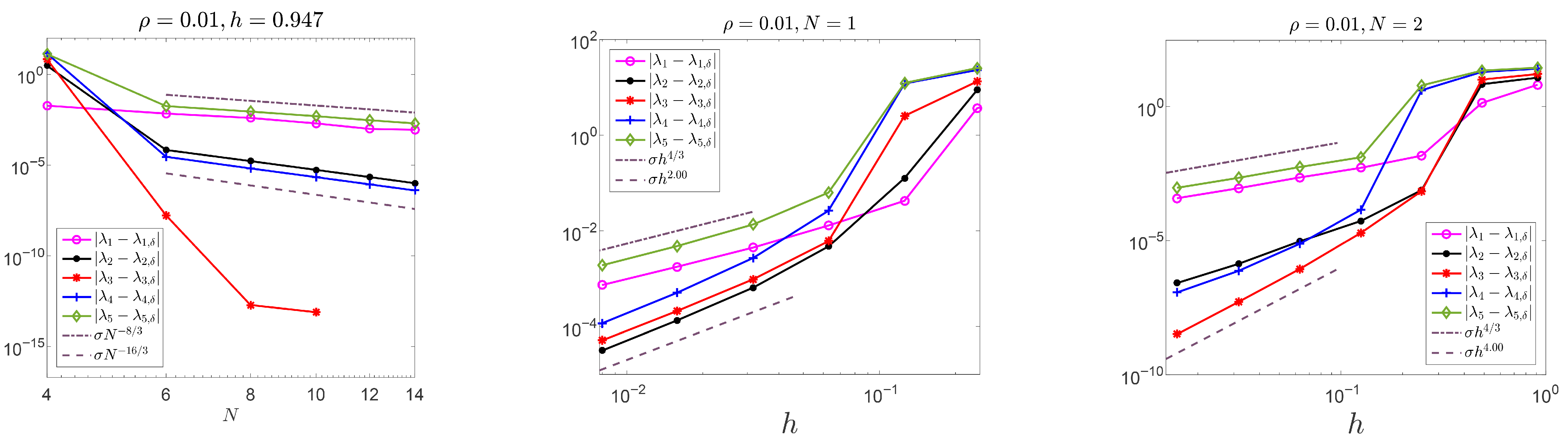
We then take $\rho =1$, $n=N$, and $m=N$. As the polynomial degree increases, Table 3 presents the corresponding errors ${\lambda }_i-{\lambda }_{i,\delta },i=1,2,\dots ,5$ in the framework of our p-version method for a fixed mesh size $h=0.963$. From this table, we observe that ${\lambda }_{i,\delta },i=1,2,\dots ,5$ converge exponentially from above to ${\lambda }_i$ with respect to the polynomial degree.

Table 3. Errors ${\lambda }_i-{\lambda }_{i,\delta }$ ($i=1,2,\dots ,5$) vs. N for $\rho =1$, $n=N$, $m=N$ on the quadrilateral mesh with $h=0.963$ of $\mathsf{\Omega }={[0,1]}^2$.

N	${\mathit{\lambda }}_1-{\mathit{\lambda }}_{1,\mathit{\delta }}$	${\mathit{\lambda }}_2-{\mathit{\lambda }}_{2,\mathit{\delta }}$	${\mathit{\lambda }}_3-{\mathit{\lambda }}_{3,\mathit{\delta }}$	${\mathit{\lambda }}_4-{\mathit{\lambda }}_{4,\mathit{\delta }}$	${\mathit{\lambda }}_5-{\mathit{\lambda }}_{5,\mathit{\delta }}$
3	−0.009	−0.466	−0.557	−1.277	0.057
4	−6.766 × 10−5	−0.012	−0.027	−0.057	−1.290
5	−4.413 × 10−6	−0.002	−0.003	−0.009	−0.019
6	−1.089 × 10−8	−3.233 × 10−5	−6.507 × 10−5	−2.368 × 10−4	−0.013
7	−4.612 × 10−10	−1.736 × 10−6	−2.784 × 10−6	−1.653 × 10−5	−7.148 × 10−5
8	−5.009 × 10−13	−2.064 × 10−8	−4.327 × 10−8	−2.398 × 10−7	−3.130 × 10−5
9	4.690 × 10−13	−5.528 × 10−10	−9.711 × 10−10	−1.015 × 10−8	−9.350 × 10−8
10	4.441 × 10−13	−4.491 × 10−12	−1.055 × 10−11	−8.944 × 10−11	−2.943 × 10−8
11	4.228 × 10−13	8.313 × 10−13	−2.842 × 10−14	−2.345 × 10−12	−5.403 × 10−11
12	−3.340 × 10−13	−3.126 × 10−13	−1.187 × 10−12	−1.563 × 10−13	−1.369 × 10−11
13	4.619 × 10−13	7.034 × 10−13	1.776 × 10−13	2.132 × 10−13	3.268 × 10−13

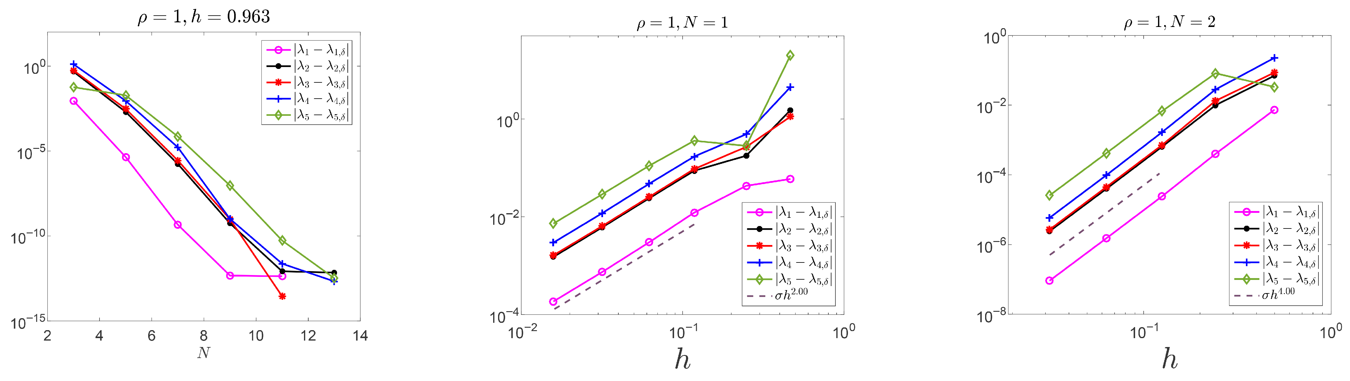
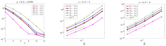
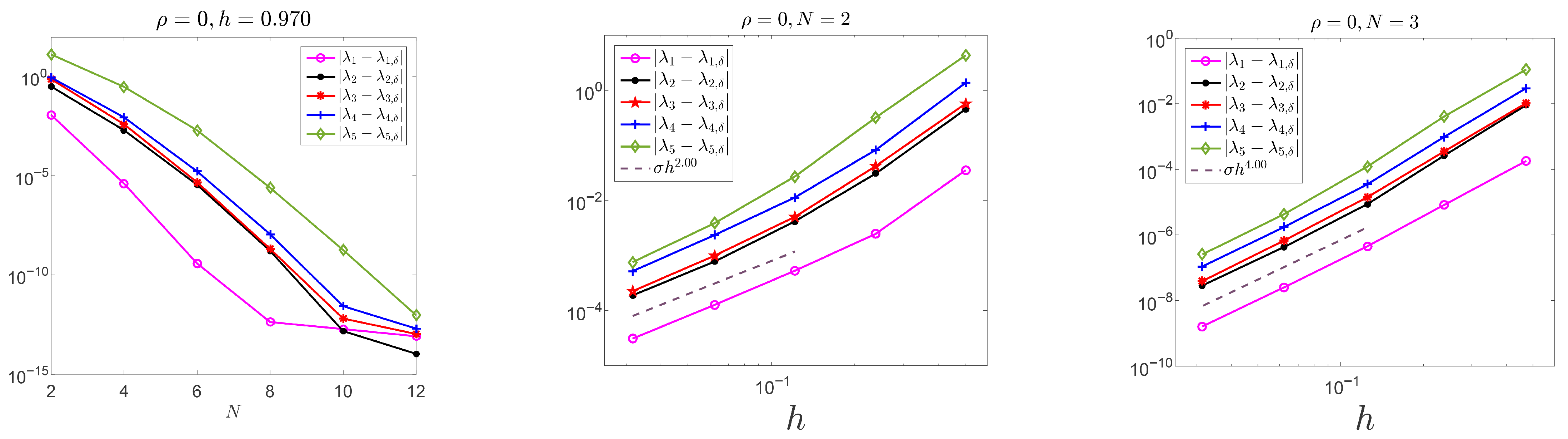
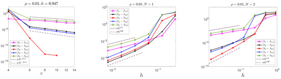
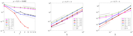
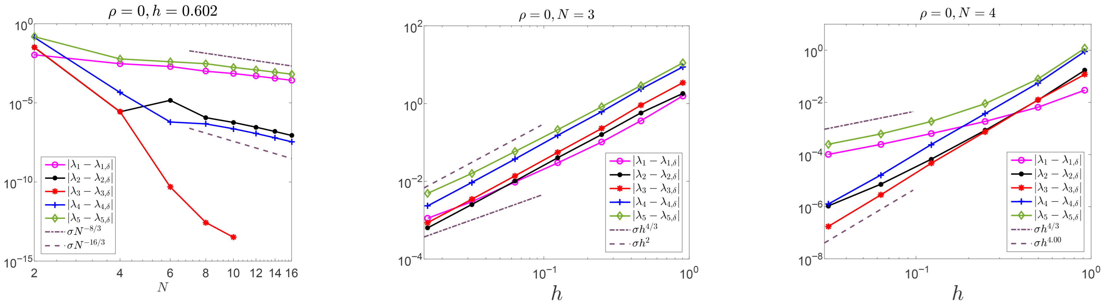
To vividly illustrate the convergence behaviors of numerical eigenvalues, we present the absolute errors $|{\lambda }_i-{\lambda }_{i,\delta }|,i=1,2,\dots ,5$ versus N in the left panel of Figure 4 in semi-log scale for $h=0.963$. These results clearly demonstrate the exponential orders of convergence of the first five numerical eigenvalues with respect to the polynomial degree.

Figure 4. Errors $|{\lambda }_i-{\lambda }_{i,\delta }|,i=1,2,\dots ,5$ for $\rho =1,n=N,m=N$ on quadrilateral meshes of $\mathsf{\Omega }={[0,1]}^2$. (Left): vs. N with $h=0.963$; (middle): vs. h with $N=1$; (right): vs. h with $N=2$.

In the framework of the h-version method, Table 4 lists the errors ${\lambda }_i-{\lambda }_{i,\delta },$$i=1,2,\dots ,5$, and the convergence rates for $N=1,2$. All the errors are observed to be negative. Moreover, as the mesh size decreases, ${\lambda }_{i,\delta }$ converge to ${\lambda }_i$ at rates of approximately $\mathcal{O}\left(h^2\right)$ for $N=1$ and $\mathcal{O}\left(h^4\right)$ for $N=2$. These findings confirm that the numerical eigenvalues obtained by the h-version method converge from above at the optimal rates in this case. To more intuitively visualize the convergence behaviors of the errors obtained by our h-version method, we also plot the absolute errors $|{\lambda }_i-{\lambda }_{i,\delta }|,i=1,2,\dots ,5$ versus h in log–log scale for $N=1$ and $N=2$ in the middle and right panels of Figure 4, respectively.

Table 4. Errors ${\lambda }_i-{\lambda }_{i,\delta }$ ($i=1,2,\dots ,5$) and convergence orders vs. h for $\rho =1$, $n=N$, $m=N$ on quadrilateral meshes of $\mathsf{\Omega }={[0,1]}^2$ with $N=1$ (top) and $N=2$ (bottom).

h	${\mathit{\lambda }}_1-{\mathit{\lambda }}_{1,\mathit{\delta }}$	Order	${\mathit{\lambda }}_2-{\mathit{\lambda }}_{2,\mathit{\delta }}$	Order	${\mathit{\lambda }}_3-{\mathit{\lambda }}_{3,\mathit{\delta }}$	Order	${\mathit{\lambda }}_4-{\mathit{\lambda }}_{4,\mathit{\delta }}$	Order	${\mathit{\lambda }}_5-{\mathit{\lambda }}_{5,\mathit{\delta }}$	Order
0.232	−0.045	–	−0.227	–	−0.324	−	−0.492	–	0.560	–
0.124	−0.012	2.105	1.543	2.002	−0.101	1.851	−0.176	1.631	−0.328	0.851
0.062	−0.003	2.009	−0.024	1.843	−0.026	1.977	−0.048	1.878	−0.108	1.594
0.032	−7.402 × 10−4	2.063	−0.006	2.052	−0.007	2.021	−0.012	2.071	−0.029	1.978
0.016	−1.856 × 10−4	2.033	−0.002	2.020	−0.002	2.052	−0.003	2.042	−0.007	2.021
$\mathit{h}$	${\mathit{\lambda }}_{\mathbf{1}}-{\mathit{\lambda }}_{\mathbf{1},\mathit{\delta }}$	order	${\mathit{\lambda }}_{\mathbf{2}}-{\mathit{\lambda }}_{\mathbf{2},\mathit{\delta }}$	order	${\mathit{\lambda }}_{\mathbf{3}}-{\mathit{\lambda }}_{\mathbf{3},\mathit{\delta }}$	order	${\mathit{\lambda }}_{\mathbf{4}}-{\mathit{\lambda }}_{\mathbf{4},\mathit{\delta }}$	order	${\mathit{\lambda }}_{\mathbf{5}}-{\mathit{\lambda }}_{\mathbf{5},\mathit{\delta }}$	order
0.477	−0.014	–	−0.262	–	−0.306	–	−0.685	–	−2.848	–
0.252	−0.001	4.001	−0.024	3.751	−0.030	3.651	−0.064	3.718	−0.234	3.923
0.123	−5.813 × 10−5	4.117	−0.002	3.793	−0.002	3.988	−0.004	3.931	−0.015	3.791
0.063	−3.666 × 10−6	4.124	−9.700 × 10−5	4.163	−1.058 × 10−4	4.150	−2.301 × 10−4	4.191	−1.035 × 10−3	4.029
0.032	−2.278 × 10−7	4.019	−5.907 × 10−6	4.048	−1.459 × 10−5	3.990	−6.242 × 10−5	4.063	−6.408 × 10−6	4.056

4.2.2. In the Case of $\rho =0$

Let us explore the upper- and lower-bound approximations of numerical eigenvalues on convex quadrilateral meshes of $\mathsf{\Omega }={[0,1]}^2$ in the case of $\rho =0$.

The numerical eigenvalues are the upper bounds of the exact eigenvalues in both our h- and p-version methods

• If $n\le N-1$ and $m\le N$ for $\rho =0$.

In the following, we take the numerical results of $n=N-1$, $m=N$ as examples for validation.

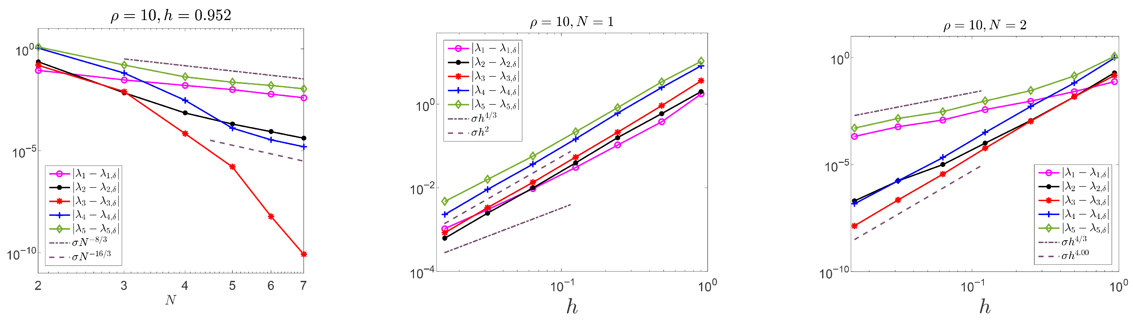
In Table 5, we tabulate the errors ${\lambda }_i-{\lambda }_{i,\delta },i=1,2,\dots ,5$ obtained by the p-version weak Galerkin spectral element method with the fixed mesh size $h=0.970$. It can be observed that as the polynomial degree increases, ${\lambda }_{i,\delta }$ converge exponentially from above to ${\lambda }_i$.

Table 5. Errors ${\lambda }_i-{\lambda }_{i,\delta }$ ($i=1,2,\dots ,5$) vs. N for $\rho =0$, $n=N-1$, $m=N$ on the quadrilateral mesh with $h=0.970$ of $\mathsf{\Omega }={[0,1]}^2$.

N	${\mathit{\lambda }}_1-{\mathit{\lambda }}_{1,\mathit{\delta }}$	${\mathit{\lambda }}_2-{\mathit{\lambda }}_{2,\mathit{\delta }}$	${\mathit{\lambda }}_3-{\mathit{\lambda }}_{3,\mathit{\delta }}$	${\mathit{\lambda }}_4-{\mathit{\lambda }}_{4,\mathit{\delta }}$	${\mathit{\lambda }}_5-{\mathit{\lambda }}_{5,\mathit{\delta }}$
2	−0.012	−0.324	−0.767	−0.913	−13.48
3	−8.636 × 10−4	−0.076	−0.088	−0.248	−0.571
4	−4.104 × 10−6	−0.002	−0.004	−0.009	−0.309
5	−2.406 × 10−7	−1.426 × 10−4	−1.630 × 10−4	−0.001	−0.006
6	−3.841 × 10−10	−3.558 × 10−6	−4.779 × 10−6	−1.699 × 10−5	−0.002
7	−2.031 × 10−11	−8.277 × 10−8	−9.598 × 10−8	−1.359 × 10−6	−1.648 × 10−5
8	4.263 × 10−13	−1.660 × 10−9	−2.087 × 10−9	−1.143 × 10−8	−2.516 × 10−6
9	1.741 × 10−13	−2.058 × 10−11	−2.412 × 10−11	−6.779 × 10−10	−1.904 × 10−8
10	−1.883 × 10−13	−1.492 × 10−13	−6.395 × 10−13	−2.700 × 10−12	−1.831 × 10−9
11	−2.451 × 10−13	−4.974 × 10−14	−3.837 × 10−13	4.263 × 10−14	−1.064 × 10−11
12	8.171 × 10−14	−1.066 × 10−14	−1.066 × 10−13	−1.990 × 10−13	−9.379 × 10−13

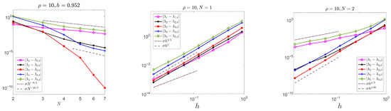
To vividly demonstrate the convergence behaviors of numerical eigenvalues with respect to the polynomial degree, the left panel of Figure 5 displays the absolute errors $|{\lambda }_i-{\lambda }_{i,\delta }|,i=1,2,\dots ,5$ versus N in semi-log scale for the fixed mesh size $h=0.970$, which clearly reveals the expected exponential convergence rates.

Figure 5. Errors $|{\lambda }_i-{\lambda }_{i,\delta }|,i=1,2,\dots ,5$ for $\rho =0,n=N-1,m=N$ on quadrilateral meshes of $\mathsf{\Omega }={[0,1]}^2$. (Left): vs. N with $h=0.970$; (middle): vs. h with $N=2$; (right): vs. h with $N=3$.

Furthermore, Table 6 lists the errors ${\lambda }_i-{\lambda }_{i,\delta },i=1,2,\dots ,5$, and the convergence rates in the h-version method for $N=2,3$. It is observed that ${\lambda }_{i,\delta }$ converge from above, as evidenced by the negative errors, at rates of approximately $\mathcal{O}\left(h^2\right)$ for $N=2$ and $\mathcal{O}\left(h^4\right)$ for $N=3$. In addition, the convergence behaviors of the h-version method is further illustrated in Figure 5. The middle and right panels of Figure 5 display the absolute errors $|{\lambda }_i-{\lambda }_{i,\delta }|,i=1,2,\dots ,5$ versus h in log–log scale for $N=2$ and $N=3$, respectively. These plots clearly demonstrate the optimal convergence orders of the h-version method with respect to the mesh size.

Table 6. Errors ${\lambda }_i-{\lambda }_{i,\delta }$ ($i=1,2,\dots ,5$) and convergence orders vs. h for $\rho =0$, $n=N-1$, $m=N$ on quadrilateral meshes of $\mathsf{\Omega }={[0,1]}^2$ with $N=2$ (top) and $N=3$ (bottom).

h	${\mathit{\lambda }}_1-{\mathit{\lambda }}_{1,\mathit{\delta }}$	Order	${\mathit{\lambda }}_2-{\mathit{\lambda }}_{2,\mathit{\delta }}$	Order	${\mathit{\lambda }}_3-{\mathit{\lambda }}_{3,\mathit{\delta }}$	Order	${\mathit{\lambda }}_4-{\mathit{\lambda }}_{4,\mathit{\delta }}$	Order	${\mathit{\lambda }}_5-{\mathit{\lambda }}_{5,\mathit{\delta }}$	Order
0.459	−0.026	–	−0.421	–	−0.651	–	−0.855	–	−3.704	–
0.251	−0.003	3.577	−0.040	3.161	−0.042	3.165	−0.105	3.122	−0.317	3.700
0.126	−6.580 × 10−4	2.512	−0.005	3.055	−0.005	3.040	−0.013	3.231	−0.033	3.428
0.064	−1.351 × 10−4	2.103	−7.898 × 10−4	2.762	−9.975 × 10−4	2.700	−0.002	2.630	−0.004	3.274
0.032	−3.302 × 10−5	2.020	−1.844 × 10−4	2.150	−2.442 × 10−4	2.111	−5.434 × 10−4	2.096	−7.320 × 10−4	2.466
0.008	−2.046 × 10−6	2.023	−1.109 × 10−5	2.039	−1.456 × 10−5	2.003	−3.292 × 10−5	2.096	−4.187 × 10−5	2.013
$\mathit{h}$	${\mathit{\lambda }}_{\mathbf{1}}-{\mathit{\lambda }}_{\mathbf{1},\mathit{\delta }}$	order	${\mathit{\lambda }}_{\mathbf{2}}-{\mathit{\lambda }}_{\mathbf{2},\mathit{\delta }}$	order	${\mathit{\lambda }}_{\mathbf{3}}-{\mathit{\lambda }}_{\mathbf{3},\mathit{\delta }}$	order	${\mathit{\lambda }}_{\mathbf{4}}-{\mathit{\lambda }}_{\mathbf{4},\mathit{\delta }}$	order	${\mathit{\lambda }}_{\mathbf{5}}-{\mathit{\lambda }}_{\mathbf{5},\mathit{\delta }}$	order
0.738	−0.003	–	−0.027	–	−0.031	–	−0.058	–	−4.761	–
0.461	−1.474 × 10−4	6.290	−0.007	2.748	−0.014	1.635	−0.024	1.836	−0.153	7.297
0.238	−6.934 × 10−6	4.633	−2.628 × 10−4	5.062	−2.975 × 10−4	5.852	−0.001	4.713	−0.004	5.400
0.127	−4.926 × 10−7	4.214	−8.426 × 10−6	5.482	−1.544 × 10−5	4.714	−3.617 × 10−5	5.431	−1.012 × 10−4	5.991
0.061	−2.539 × 10−8	4.070	−4.381 × 10−7	4.058	−5.910 × 10−7	4.479	−1.755 × 10−6	4.153	−4.390 × 10−6	4.306
0.031	−1.768 × 10−9	3.940	−2.981 × 10−8	3.974	−4.240 × 10−8	3.896	−1.136 × 10−7	4.048	−2.599 × 10−7	4.180

4.3. Numerical Study on L-Shaped Domain

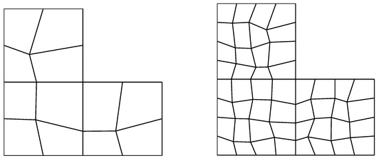
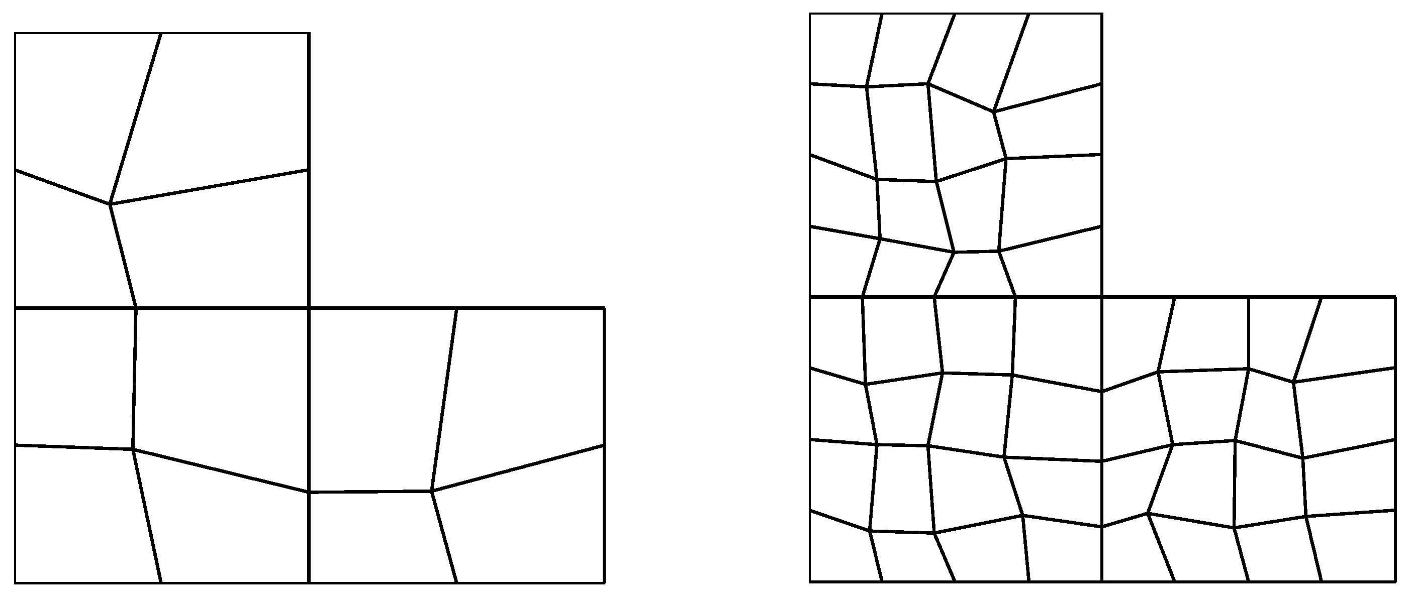
In this subsection, we examine the upper- and lower-bound approximations of numerical eigenvalues by the weak Galerkin spectral element method for the problem (6) on quadrilateral meshes of the L-shaped domain $\mathsf{\Omega }={[-1,1]}^2\setminus {[0,1]}^2$. Figure 6 illustrates the computational domain $\mathsf{\Omega }={[-1,1]}^2\setminus {[0,1]}^2$ and the quadrilateral meshes with mesh sizes $h=0.943$ and $h=0.487$.

Figure 6. Computational domain $\mathsf{\Omega }={[-1,1]}^2\setminus {[0,1]}^2$ and quadrilateral meshes with mesh sizes $h=0.943$ (left) and $h=0.487$ (right).

Notably, the concave corner with an interior angle of ${\displaystyle \frac{3\pi }{2}}$ on the L-shaped domain may lead to the corner singularities of some eigenfunctions, which causes the corresponding eigenvalues to converge at limited convergence rates. Specifically, the eigenfunction $u_1$ corresponding to the smallest eigenvalue ${\lambda }_1$ possesses a singularity of type $r^{{\displaystyle \frac{2}{3}}}$ with $r=\sqrt{x^2+y^2}$. One derives from [27] that $u_1\in H^{{\displaystyle \frac{5}{3}}-\sigma }\left(\mathsf{\Omega }\right),\forall \sigma >0$ and $u_1\in B^{{\displaystyle \frac{7}{3}}}\left(\mathsf{\Omega }\right)$, where $B^s\left(\mathsf{\Omega }\right)$ denotes the Besov space of order s. Therefore, the convergence rate of ${\lambda }_{1,\delta }$, obtained by the h-version method, is bounded above by $\mathcal{O}(h^{\frac{4}{3}})$. Meanwhile, the p-version method can achieve the convergence rate $\mathcal{O}(N^{-\frac{8}{3}})$.

For comparison with the numerical eigenvalues, we take the first five smallest eigenvalues reported in [28] as the reference eigenvalues:

$$\begin{array}{cc}\hfill & {\lambda }_1\approx 9.63972384402194105271,{\lambda }_2\approx 15.19725192645434327488,{\lambda }_3=2{\pi }^2,\hfill \\ \hfill & {\lambda }_4\approx 29.52148111414488329822,{\lambda }_5\approx 31.91263595713776220033,\hfill \end{array}$$

in which the third eigenvalue ${\lambda }_3$ is formulated exactly.

Next, we discuss the cases $\rho >0$ and $\rho =0$ separately as well.

4.3.1. In the Case of $\rho >0$

It follows from Theorem 1 that the approximation scheme (8) is well-posed for $\rho >0$ if $n\le N$ and $m\in {\mathbb{N}}_0$.

The numerical eigenvalues are observed to converge from below to the reference eigenvalues in both h- and p-version methods

• If $n=N$, and $m\ge N$ for a proper $\rho >0$, such as $\rho \le 0.01$.

Furthermore, the numerical eigenvalues are observed to converge from above to the reference eigenvalues in both h- and p-version methods

• If $n=N$, and $m\ge N$ for a proper $\rho >0$, such as $\rho \ge 10$.

In what follows, we select appropriate $\rho$, n, and m to illustrate the upper- and lower-bound approximations of numerical eigenvalues on convex quadrilateral meshes of $\mathsf{\Omega }={[-1,1]}^2\setminus {[0,1]}^2$.

We first take $\rho =0.01$, $n=N$, and $m=N+1$. The corresponding errors ${\lambda }_i-{\lambda }_{i,\delta },$$i=1,2,\dots ,5$, obtained by the p-version method for $h=0.947$ and $h=0.675$ are presented in Table 7. As observed from this table, the numerical eigenvalues ${\lambda }_{1,\delta }$ and ${\lambda }_{5,\delta }$ converge to the reference ones at a rate around $N^{-8/3}$, while the numerical eigenvalues ${\lambda }_{2,\delta }$ and ${\lambda }_{4,\delta }$ converge at a rate around $N^{-16/3}$, and the numerical eigenvalue ${\lambda }_{3,\delta }$ converges at an exponential rate. More importantly, all these errors are positive during the approximation process. These observations indicate that, in this case, ${\lambda }_{i,\delta }$ converge from below to ${\lambda }_i$ with respect to the polynomial degree.

Table 7. Errors ${\lambda }_i-{\lambda }_{i,\delta }$ ($i=1,2,\dots ,5$) and convergence orders vs. N for $\rho =0.01$, $n=N$, $m=N+1$ on quadrilateral meshes of $\mathsf{\Omega }={[-1,1]}^2\setminus {[0,1]}^2$ with $h=0.947$ (top) and $h=0.675$ (bottom).

N	${\mathit{\lambda }}_1-{\mathit{\lambda }}_{1,\mathit{\delta }}$	Order	${\mathit{\lambda }}_2-{\mathit{\lambda }}_{2,\mathit{\delta }}$	Order	${\mathit{\lambda }}_4-{\mathit{\lambda }}_{4,\mathit{\delta }}$	Order	${\mathit{\lambda }}_5-{\mathit{\lambda }}_{5,\mathit{\delta }}$	Order	${\mathit{\lambda }}_3-{\mathit{\lambda }}_{3,\mathit{\delta }}$
4	0.019	–	3.044	–	14.32	–	13.32	–	6.854
6	0.007	−2.390	6.881 × 10−5	−5.021	2.896 × 10−5	−69.01	0.018	−34.43	1.713 × 10−8
8	0.004	−2.441	1.671 × 10−5	−4.938	6.612 × 10−6	−4.940	0.009	−2.438	1.954 × 10−13
10	0.002	−2.475	5.503 × 10−6	−4.990	2.185 × 10−6	−4.977	0.005	−2.474	7.816 × 10−14
12	0.001	−2.500	2.204 × 10−6	−5.029	8.766 × 10−7	−5.021	0.003	−2.500	2.629 × 10−13
14	8.966 × 10−4	−2.519	1.011 × 10−6	−5.059	4.027 × 10−7	−5.055	0.002	−2.519	−3.553 × 10−15
$\mathit{N}$	${\mathit{\lambda }}_{\mathbf{1}}-{\mathit{\lambda }}_{\mathbf{1},\mathit{\delta }}$	order	${\mathit{\lambda }}_{\mathbf{2}}-{\mathit{\lambda }}_{\mathbf{2},\mathit{\delta }}$	order	${\mathit{\lambda }}_{\mathbf{4}}-{\mathit{\lambda }}_{\mathbf{4},\mathit{\delta }}$	order	${\mathit{\lambda }}_{\mathbf{5}}-{\mathit{\lambda }}_{\mathbf{5},\mathit{\delta }}$	order	${\mathit{\lambda }}_{\mathbf{3}}-{\mathit{\lambda }}_{\mathbf{3},\mathit{\delta }}$
4	0.012	–	1.926 × 10−4	–	6.194	–	5.557	–	1.485 × 10−5
6	0.004	−2.390	2.605 × 10−5	−4.875	1.024 × 10−5	−5.251	0.011	−2.386	7.043 × 10−11
8	0.002	−2.441	6.312 × 10−6	−4.945	2.498 × 10−6	−4.922	0.005	−2.440	1.634 × 10−13
10	0.001	−2.475	2.076 × 10−6	−4.995	8.245 × 10−7	−4.982	0.003	−2.475	−5.684 × 10−14
12	8.020 × 10−4	−2.500	8.309 × 10−7	−5.032	3.305 × 10−7	−5.025	0.002	−2.500	5.826 × 10−13
14	5.443 × 10−4	−2.519	3.812 × 10−7	−5.063	1.517 × 10−7	−5.055	0.001	−2.519	2.345 × 10−13

We then plot the corresponding absolute errors $|{\lambda }_i-{\lambda }_{i,\delta }|,i=1,2,\dots ,5$, versus N in the left part of Figure 7 in log–log scale for $h=0.947$, which clearly shows that the first five numerical eigenvalues converge at the expected convergence orders with respect to the polynomial degree.

Figure 7. Errors $|{\lambda }_i-{\lambda }_{i,\delta }|,i=1,2,\dots ,5$ for $\rho =0.01,n=N,m=N+1$ on quadrilateral meshes of $\mathsf{\Omega }={[-1,1]}^2\setminus {[0,1]}^2$. (Left): vs. N with $h=0.947$; (middle): vs. h with $N=1$; (right): vs. h with $N=2$.

Furthermore, in the h-version method, we present the errors ${\lambda }_i-{\lambda }_{i,\delta },i=1,2,\dots ,5$, and the convergence rates for $N=1,2$ in Table 8. It can be observed that all tabulated errors are positive, which indicates that ${\lambda }_{i,\delta }$ are the lower-bound approximations of ${\lambda }_i$. To provide a more intuitive visualization of the convergence behaviors of numerical eigenvalues, we also plot the absolute errors $|{\lambda }_i-{\lambda }_{i,\delta }|,i=1,2,\dots ,5$ versus h in log–log scale for $N=1$ and $N=2$ in the middle and right panels of Figure 7, respectively, where expected convergence orders can be observed with respect to the mesh size.

Table 8. Errors ${\lambda }_i-{\lambda }_{i,\delta }$ ($i=1,2,\dots ,5$) and convergence orders vs. h for $\rho =0.01$, $n=N$, $m=N+1$ on quadrilateral meshes of $\mathsf{\Omega }={[-1,1]}^2\setminus {[0,1]}^2$ with $N=1$ (top) and $N=2$ (bottom).

h	${\mathit{\lambda }}_1-{\mathit{\lambda }}_{1,\mathit{\delta }}$	Order	${\mathit{\lambda }}_2-{\mathit{\lambda }}_{2,\mathit{\delta }}$	Order	${\mathit{\lambda }}_3-{\mathit{\lambda }}_{3,\mathit{\delta }}$	Order	${\mathit{\lambda }}_4-{\mathit{\lambda }}_{4,\mathit{\delta }}$	Order	${\mathit{\lambda }}_5-{\mathit{\lambda }}_{5,\mathit{\delta }}$	Order
0.115	0.037	–	0.089	–	2.125	–	11.17	–	12.26	–
0.061	0.012	1.753	0.004	4.774	0.006	9.316	0.023	9.676	0.058	8.400
0.031	0.004	1.602	6.297 × 10−4	2.817	9.208 × 10−4	2.670	0.003	3.242	0.013	2.257
0.016	0.002	1.272	1.318 × 10−4	2.338	2.070 × 10−4	2.231	4.958 × 10−4	2.484	0.005	1.463
0.008	6.254 × 10−4	1.479	3.110 × 10−5	2.077	5.076 × 10−5	2.022	1.169 × 10−4	2.079	0.002	1.530
$\mathit{h}$	${\mathit{\lambda }}_{\mathbf{1}}-{\mathit{\lambda }}_{\mathbf{1},\mathit{\delta }}$	order	${\mathit{\lambda }}_{\mathbf{2}}-{\mathit{\lambda }}_{\mathbf{2},\mathit{\delta }}$	order	${\mathit{\lambda }}_{\mathbf{3}}-{\mathit{\lambda }}_{\mathbf{3},\mathit{\delta }}$	order	${\mathit{\lambda }}_{\mathbf{4}}-{\mathit{\lambda }}_{\mathbf{4},\mathit{\delta }}$	order	${\mathit{\lambda }}_{\mathbf{5}}-{\mathit{\lambda }}_{\mathbf{5},\mathit{\delta }}$	order
0.389	0.034	–	4.379	–	8.300	–	14.84	–	16.86	–
0.220	0.012	1.820	5.003 × 10−4	15.93	3.601 × 10−4	17.63	0.012	12.56	0.125	8.606
0.116	0.005	1.354	5.395 × 10−5	3.460	1.443 × 10−5	4.998	1.086 × 10−4	7.252	0.013	3.569
0.061	0.002	1.353	7.885 × 10−6	3.033	7.477 × 10−7	4.668	6.594 × 10−6	4.418	0.005	1.366
0.031	9.375 × 10−4	1.231	1.546 × 10−6	2.400	4.908 × 10−8	4.011	8.085 × 10−7	3.091	0.002	1.232
0.016	3.571 × 10−4	1.430	2.211 × 10−7	2.882	3.139 × 10−9	4.075	1.002 × 10−7	3.095	8.722 × 10−4	1.430

To explore the upper bound approximations of numerical eigenvalues, we then select $\rho =10$, $n=N$, and $m=N+1$ in the following numerical experiments. In Table 9, we present the errors ${\lambda }_i-{\lambda }_{i,\delta },i=1,2,\dots ,5$, and the convergence orders obtained by the p-version method for $h=0.952$ and $h=0.655$. Furthermore, the absolute errors $|{\lambda }_i-{\lambda }_{i,\delta }|,i=1,2,\dots ,5$ versus N are plotted in the left panel of Figure 8 in log–log scale for $h=0.952$. From this table and figure, we observe that the numerical eigenvalues approximate the exact eigenvalues from above at the theoretical rates with respect to the polynomial degree.

Table 9. Errors ${\lambda }_i-{\lambda }_{i,\delta }$ ($i=1,2,\dots ,5$) and convergence orders vs. N for $\rho =10$, $n=N$, $m=N+1$ on quadrilateral meshes of $\mathsf{\Omega }={[-1,1]}^2\setminus {[0,1]}^2$ with $h=0.952$ (top) and $h=0.655$ (bottom).

N	${\mathit{\lambda }}_1-{\mathit{\lambda }}_{1,\mathit{\delta }}$	Order	${\mathit{\lambda }}_2-{\mathit{\lambda }}_{2,\mathit{\delta }}$	Order	${\mathit{\lambda }}_4-{\mathit{\lambda }}_{4,\mathit{\delta }}$	Order	${\mathit{\lambda }}_5-{\mathit{\lambda }}_{5,\mathit{\delta }}$	Order	${\mathit{\lambda }}_3-{\mathit{\lambda }}_{3,\mathit{\delta }}$
2	−0.088	–	−0.233	–	−1.094	–	−1.240	–	−0.156
3	−0.030	−2.700	−0.007	−8.727	−0.065	−6.957	−0.161	−5.036	−0.008
4	−0.016	−2.192	−7.153 × 10−4	−7.816	−0.003	−10.41	−0.042	−4.690	−6.954 × 10−5
5	−0.010	−2.181	−2.044 × 10−4	−5.614	−1.288 × 10−4	−14.49	−0.023	−2.576	−1.615 × 10−6
6	−0.006	−2.256	−8.666 × 10−5	−4.706	−3.436 × 10−5	−7.246	−0.016	−2.253	−6.071 × 10−9
7	−0.004	−2.308	−4.134 × 10−5	−4.801	−1.580 × 10−5	−5.040	−0.011	−2.295	−8.381 × 10−11
$\mathit{N}$	${\mathit{\lambda }}_{\mathbf{1}}-{\mathit{\lambda }}_{\mathbf{1},\mathit{\delta }}$	order	${\mathit{\lambda }}_{\mathbf{2}}-{\mathit{\lambda }}_{\mathbf{2},\mathit{\delta }}$	order	${\mathit{\lambda }}_{\mathbf{4}}-{\mathit{\lambda }}_{\mathbf{4},\mathit{\delta }}$	order	${\mathit{\lambda }}_{\mathbf{5}}-{\mathit{\lambda }}_{\mathbf{5},\mathit{\delta }}$	order	${\mathit{\lambda }}_{\mathbf{3}}-{\mathit{\lambda }}_{\mathbf{3},\mathit{\delta }}$
2	−0.045	–	−0.054	–	−0.193	–	−0.271	–	−0.044
3	−0.017	−2.416	−0.001	−9.523	−0.010	−7.277	−0.056	−3.891	−8.203 × 10−4
4	−0.009	−2.110	−2.067 × 10−4	−5.908	−1.495 × 10−4	−14.64	−0.022	−3.203	−5.381 × 10−6
5	−0.006	−2.195	−7.035 × 10−5	−4.831	−2.898 × 10−5	−7.352	−0.014	−2.178	−4.561 × 10−8
6	−0.004	−2.263	−2.953 × 10−5	−4.761	−1.137 × 10−5	−5.134	−0.009	−2.252	−1.240 × 10−10
7	−0.003	−2.313	−1.405 × 10−5	−4.818	−5.465 × 10−6	−4.750	−0.007	−2.304	5.898 × 10−13

Figure 8. Errors $|{\lambda }_i-{\lambda }_{i,\delta }|,i=1,2,\dots ,5$ for $\rho =10,n=N,m=N+1$ on quadrilateral meshes of $\mathsf{\Omega }={[-1,1]}^2\setminus {[0,1]}^2$. (Left): vs. N with $h=0.952$; (middle): vs. h with $N=1$; (right): vs. h with $N=2$.

In addition, we use the h-version weak Galerkin spectral element method with $\rho =10$, $n=N$, $m=N+1$ to solve the problem (6) and present the errors ${\lambda }_i-{\lambda }_{i,\delta },i=1,2,\dots ,5$, as well as the corresponding convergence rates, for polynomial degrees $N=1$ and $N=2$ in Table 10. It can be observed that ${\lambda }_{i,\delta }$ converge to ${\lambda }_i$ from above at the predicted rates as the mesh size h decreases. Besides, the convergence behaviors are further illustrated in the middle and right panels of Figure 8, where the absolute errors $|{\lambda }_i-{\lambda }_{i,\delta }|,i=1,2,\dots ,5$, are plotted versus h in log–log scale for $N=1$ and $N=2$, respectively.

Table 10. Errors ${\lambda }_i-{\lambda }_{i,\delta }$ ($i=1,2,\dots ,5$) and convergence orders vs. h for $\rho =10$, $n=N$, $m=N+1$ on quadrilateral meshes of $\mathsf{\Omega }={[-1,1]}^2\setminus {[0,1]}^2$ with $N=1$ (top) and $N=2$ (bottom).

h	${\mathit{\lambda }}_1-{\mathit{\lambda }}_{1,\mathit{\delta }}$	Order	${\mathit{\lambda }}_2-{\mathit{\lambda }}_{2,\mathit{\delta }}$	Order	${\mathit{\lambda }}_3-{\mathit{\lambda }}_{3,\mathit{\delta }}$	Order	${\mathit{\lambda }}_4-{\mathit{\lambda }}_{4,\mathit{\delta }}$	Order	${\mathit{\lambda }}_5-{\mathit{\lambda }}_{5,\mathit{\delta }}$	Order
0.635	−0.679	–	−0.922	–	−1.443	–	−4.077	–	−5.166	–
0.395	−0.249	2.285	−0.389	1.894	−0.611	1.995	−1.617	2.069	−2.052	2.021
0.222	−0.082	1.894	−0.123	1.932	−0.169	2.066	−0.475	2.007	−0.636	2.065
0.120	−0.026	1.780	−0.035	1.997	−0.048	2.061	−0.130	2.040	−0.186	1.953
0.061	−0.009	1.687	−0.009	2.082	−0.013	2.039	−0.034	2.074	−0.054	1.907
0.031	−0.003	1.618	−0.002	2.015	−0.003	2.034	−0.009	2.024	−0.015	1.844
0.016	−0.001	1.473	−6.102 × 10−4	2.013	−8.243 × 10−4	2.001	−0.002	2.010	−0.005	1.729
$\mathit{h}$	${\mathit{\lambda }}_{\mathbf{1}}-{\mathit{\lambda }}_{\mathbf{1},\mathit{\delta }}$	order	${\mathit{\lambda }}_{\mathbf{2}}-{\mathit{\lambda }}_{\mathbf{2},\mathit{\delta }}$	order	${\mathit{\lambda }}_{\mathbf{3}}-{\mathit{\lambda }}_{\mathbf{3},\mathit{\delta }}$	order	${\mathit{\lambda }}_{\mathbf{4}}-{\mathit{\lambda }}_{\mathbf{4},\mathit{\delta }}$	order	${\mathit{\lambda }}_{\mathbf{5}}-{\mathit{\lambda }}_{\mathbf{5},\mathit{\delta }}$	order
0.644	−0.044	–	−0.054	–	−0.048	–	−0.247	–	−0.303	–
0.395	−0.020	1.579	−0.007	4.161	−0.007	4.068	−0.031	4.237	−0.081	2.695
0.218	−0.007	1.892	−6.835 × 10−4	3.927	−6.631 × 10−4	3.845	−0.003	3.933	−0.020	2.368
0.117	−0.003	1.158	−7.788 × 10−5	3.519	−4.748 × 10−5	4.272	−2.555 × 10−4	3.979	−0.008	1.440
0.062	−0.001	1.476	−9.903 × 10−6	3.226	−3.235 × 10−6	4.202	−1.924 × 10−5	4.046	−0.003	1.515
0.031	−5.276 × 10−4	1.260	−1.413 × 10−6	2.834	−2.103 × 10−7	3.978	−1.587 × 10−6	3.631	−0.001	1.269
0.016	−2.225 × 10−4	1.264	−2.252 × 10−7	2.688	−1.346 × 10−7	4.024	−1.547 × 10−7	3.408	−5.435 × 10−4	1.265

4.3.2. In the Case of $\rho =0$

From Theorem 1, we obtain that the approximation scheme (8) is well-posed for $\rho =0$ if $n\le N-1$ and $m\le N$.

Indeed, the numerical eigenvalues are the upper bounds of the reference eigenvalues in the framework of

(i)

The p-version method for smooth eigenfunctions;

(ii)

The h-version method,

provided that $n\le N-2$ and $m\le N$ for $\rho =0$. In contrast, in the p-version method for eigenfunctions with limited regularity, the corresponding numerical eigenvalues converge from below to the reference eigenvalues if $n\le N-2$ and $m\le N$ for $\rho =0$.

In the following, we take $n=N-2$ and $m=N$ as examples for illustration.

For a fixed mesh size $h=0.602$, Table 11 presents the errors ${\lambda }_i-{\lambda }_{i,\delta },i=1,2,\dots ,5$ and the convergence rates obtained by the p-version method as the polynomial degree increases. As observed from the table, the numerical eigenvalues ${\lambda }_{1,\delta }$ and ${\lambda }_{5,\delta }$ converge to the reference eigenvalues at a rate of approximately $N^{-8/3}$, the numerical eigenvalues ${\lambda }_{2,\delta }$ and ${\lambda }_{4,\delta }$ converge at a rate about $N^{-16/3}$. Since the eigenfunction corresponding to ${\lambda }_3$ is analytic on the L-shaped domain, the numerical eigenvalue ${\lambda }_{3,\delta }$ converges to the reference eigenvalue at an exponential rate. More significantly, the numerical eigenvalues ${\lambda }_{i,\delta },i=1,2,4,5$ are asymptotic lower bounds of the reference eigenvalues ${\lambda }_i$, while the third numerical eigenvalue is the upper bound of the exact eigenvalue.

Table 11. Errors ${\lambda }_i-{\lambda }_{i,\delta }$ ($i=1,2,\dots ,5$) and convergence orders vs. N for $\rho =0$, $n=N-2$, $m=N$ on quadrilateral meshes with $h=0.602$ of $\mathsf{\Omega }={[-1,1]}^2\setminus {[0,1]}^2$.

N	${\mathit{\lambda }}_1-{\mathit{\lambda }}_{1,\mathit{\delta }}$	Order	${\mathit{\lambda }}_2-{\mathit{\lambda }}_{2,\mathit{\delta }}$	Order	${\mathit{\lambda }}_4-{\mathit{\lambda }}_{4,\mathit{\delta }}$	Order	${\mathit{\lambda }}_5-{\mathit{\lambda }}_{5,\mathit{\delta }}$	Order	${\mathit{\lambda }}_3-{\mathit{\lambda }}_{3,\mathit{\delta }}$
2	−0.011	–	−0.032	–	−0.139	–	−0.154	–	−0.033
4	0.003	1.004	−2.729 × 10−5	−8.925	−4.520 × 10−5	−15.50	0.006	3.631	−2.780 × 10−6
6	0.002	−1.232	1.451 × 10−6	−1.229	6.187 × 10−7	−2.943	0.004	−1.235	−4.870 × 10−11
8	0.001	−1.693	1.167 × 10−6	−2.062	4.685 × 10−7	−2.142	0.003	−1.693	−2.736 × 10−13
10	7.168 × 10−4	−1.914	5.788 × 10−7	−3.386	2.311 × 10−7	−3.401	1.751 × 10−3	−1.914	3.197 × 10−14
12	4.962 × 10−4	−2.048	2.907 × 10−7	−3.884	1.159 × 10−7	−3.889	1.212 × 10−3	−2.048	−4.689 × 10−13
14	3.580 × 10−4	−2.140	1.546 × 10−7	−4.159	6.163 × 10−8	−4.161	8.744 × 10−4	−2.140	−4.441 × 10−13
16	2.672 × 10−4	−2.206	8.711 × 10−8	−4.339	3.473 × 10−8	−4.338	6.527 × 10−4	−2.206	−9.308 × 10−13

To exhibit the convergence behaviors of numerical eigenvalues more vividly, we also plot the absolute errors $|{\lambda }_i-{\lambda }_{i,\delta }|,i=1,2,\dots ,5$ versus N in log–log scale for $h=0.602$ in the left panel of Figure 9, where the expected convergence orders with respect to the polynomial degree can be clearly observed.

Figure 9. Errors $|{\lambda }_i-{\lambda }_{i,\delta }|,i=1,2,\dots ,5$ for $\rho =0,n=N-2,m=N$ on quadrilateral meshes of $\mathsf{\Omega }={[-1,1]}^2\setminus {[0,1]}^2$. (Left): vs. N with $h=0.602$; (middle): vs. h with $N=3$; (right): vs. h with $N=4$.

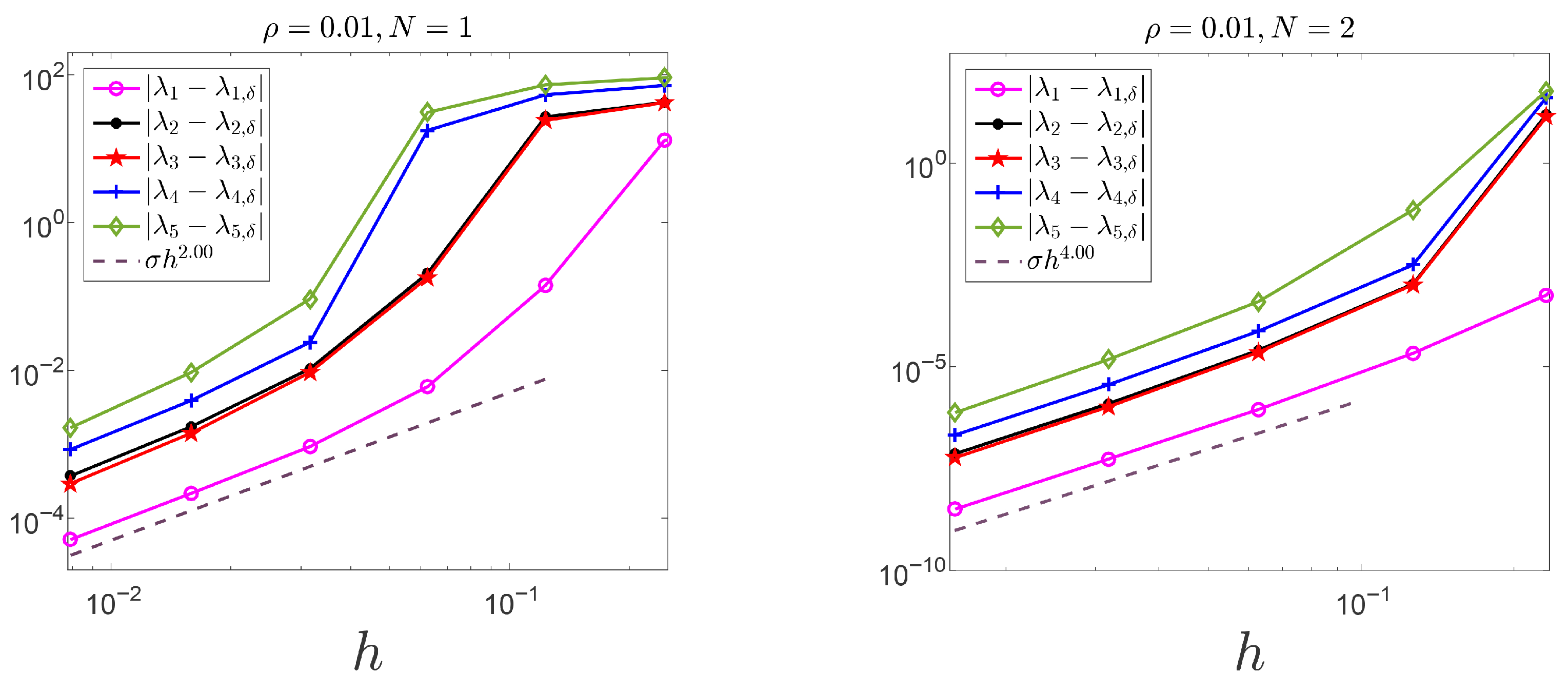
Moreover, for $\rho =0$, $n=N-2$ and $m=N$, Table 12 presents the corresponding errors ${\lambda }_i-{\lambda }_{i,\delta },i=1,2,\dots ,5$, and convergence rates obtained by the h-version method with $N=3,4$. As observed from the table, all errors are negative. Therefore, as the mesh size h decreases, ${\lambda }_{i,\delta }$ converge to ${\lambda }_i$ from above at the expected convergence rates. The convergence behaviors are further illustrated in the middle and right panels of Figure 9, where the absolute errors $|{\lambda }_i-{\lambda }_{i,\delta }|,i=1,2,\dots ,5$ are plotted versus h in log–log scale for $N=3$ and $N=4$, respectively.

Table 12. Errors ${\lambda }_i-{\lambda }_{i,\delta }$ ($i=1,2,\dots ,5$) and convergence orders vs. h for $\rho =0$, $n=N-2$, $m=N$ on quadrilateral meshes of $\mathsf{\Omega }={[-1,1]}^2\setminus {[0,1]}^2$ with $N=3$ (top) and $N=4$ (bottom).

h	${\mathit{\lambda }}_1-{\mathit{\lambda }}_{1,\mathit{\delta }}$	Order	${\mathit{\lambda }}_2-{\mathit{\lambda }}_{2,\mathit{\delta }}$	Order	${\mathit{\lambda }}_3-{\mathit{\lambda }}_{3,\mathit{\delta }}$	Order	${\mathit{\lambda }}_4-{\mathit{\lambda }}_{4,\mathit{\delta }}$	Order	${\mathit{\lambda }}_5-{\mathit{\lambda }}_{5,\mathit{\delta }}$	Order
0.659	−0.687	–	−1.075	–	−1.690	–	−4.481	–	−4.886	–
0.382	−0.246	1.880	−0.403	1.797	−0.562	2.017	−1.593	1.894	−1.885	1.745
0.219	−0.085	1.923	−0.125	2.102	−0.176	2.088	−0.495	2.104	−0.653	1.907
0.118	−0.027	1.922	−0.035	2.066	−0.049	2.105	−0.134	2.138	−0.187	2.039
0.062	−0.009	1.700	−0.010	2.010	−0.013	2.014	−0.035	2.035	−0.054	1.911
0.031	−0.003	1.465	−0.002	1.998	−0.003	2.007	−0.009	2.009	−0.016	1.772
0.016	−0.001	1.657	−6.228 × 10−4	1.980	−8.513 × 10−4	1.972	−0.002	1.979	−0.005	1.815
$\mathit{h}$	${\mathit{\lambda }}_{\mathbf{1}}-{\mathit{\lambda }}_{\mathbf{1},\mathit{\delta }}$	order	${\mathit{\lambda }}_{\mathbf{2}}-{\mathit{\lambda }}_{\mathbf{2},\mathit{\delta }}$	order	${\mathit{\lambda }}_{\mathbf{3}}-{\mathit{\lambda }}_{\mathbf{3},\mathit{\delta }}$	order	${\mathit{\lambda }}_{\mathbf{4}}-{\mathit{\lambda }}_{\mathbf{4},\mathit{\delta }}$	order	${\mathit{\lambda }}_{\mathbf{5}}-{\mathit{\lambda }}_{\mathbf{5},\mathit{\delta }}$	order
0.627	−0.013	–	−0.039	–	−0.038	–	−0.164	–	−0.205	–
0.391	−0.004	2.476	−0.005	4.326	−0.005	4.265	−0.026	3.893	−0.037	3.620
0.213	−0.001	1.728	−5.065 × 10−4	3.791	−4.789 × 10−4	3.909	−0.002	3.906	−0.006	3.003
0.119	−6.279 × 10−4	1.360	−5.553 × 10−5	3.767	−3.678 × 10−5	4.373	−1.902 × 10−4	4.352	−0.002	2.114
0.061	−2.519 × 10−4	1.367	−6.396 × 10−6	3.234	−2.502 × 10−6	4.022	−1.437 × 10−5	3.865	−6.297 × 10−4	1.517
0.031	−1.066 × 10−4	1.287	−9.013 × 10−7	2.935	−1.647 × 10−7	4.074	−1.140 × 10−6	3.795	−2.613 × 10−4	1.317
0.016	−3.740 × 10−5	1.537	−1.396 × 10−7	2.735	−1.041 × 10−8	4.049	−1.054 × 10−7	3.491	−9.142 × 10−5	1.540

5. Conclusions

This paper focuses on the investigation of the upper- and lower-bound approximations of numerical eigenvalues for the Laplacian eigenvalue problem using weak Galerkin spectral element methods on arbitrary convex quadrilateral meshes. The Piola transformation is adopted to construct the approximation space of weak gradients on each convex quadrilateral element, while a one-to-one mapping is used to establish the approximation space of weak functions. A well-posed weak Galerkin approximation scheme is established based on Galerkin approximation spaces with diverse choices of polynomial degrees. Building on this, we investigate the upper- and lower-bound approximations of numerical eigenvalues on arbitrary convex quadrilateral meshes of the square and L-shaped domains. Numerical experiments show that by suitably matching polynomial degrees in the approximation spaces and parameters in the approximation scheme, the numerical eigenvalues by the h- and p-version methods can not only achieve the optimal orders of convergence, but also exhibit upper/lower-bound approximations.

In fact, the definition of discrete weak gradients relies on the construction of the approximation space for weak gradients. Therefore, we may also construct the approximation space for weak gradients using other transformations, and further investigate how different weak gradient approximation spaces influence computational accuracy and the upper/lower bounds of numerical eigenvalues.

References

- Wang, J.P.; Ye, X. A weak Galerkin finite element method for second-order elliptic problems. J. Comput. Appl. Math. 2013, 241, 103–115. [Google Scholar] [CrossRef] [Scilit]
- Wang, J.P.; Ye, X. A weak Galerkin mixed finite element method for second order elliptic problems. Math. Comput. 2014, 83, 2101–2126. [Google Scholar] [CrossRef] [Scilit]
- Wang, J.P.; Wang, R.S.; Zhai, Q.L.; Zhang, R. A systematic study on weak Galerkin finite element methods for second order elliptic problems. J. Sci. Comput. 2018, 74, 1369–1396. [Google Scholar] [CrossRef] [Scilit]
- Mu, L.; Wang, J.P.; Ye, X. A weak Galerkin finite element method with polynomial reduction. J. Comput. Appl. Math. 2015, 285, 45–58. [Google Scholar] [CrossRef] [Scilit]
- Harris, A.; Harris, S. Superconvergence of weak Galerkin finite element approximation for second order elliptic problems by L2-projections. Appl. Math. Comput. 2014, 227, 610–621. [Google Scholar] [CrossRef] [Scilit]
- Cao, W.X.; Wang, C.M.; Wang, J.P. An Lp-primal-dual weak Galerkin method for convection-diffusion equations. J. Comput. Appl. Math. 2023, 419, 114698. [Google Scholar] [CrossRef] [Scilit]
- Li, D.; Wang, C.M.; Wang, J.P.; Ye, X. Generalized weak Galerkin finite element methods for second order elliptic problems. J. Comput. Appl. Math. 2024, 445, 115833. [Google Scholar] [CrossRef] [Scilit]
- Zhai, Q.L.; Xie, H.H.; Zhang, R.; Zhang, Z.M. The weak Galerkin method for elliptic eigenvalue problems. Commun. Comput. Phys. 2019, 26, 160–191. [Google Scholar] [CrossRef] [Scilit]
- Liang, Q.G.; Xu, X.J.; Yuan, L.Y. A weak Galerkin finite element method can compute both upper and lower eigenvalue bounds. J. Sci. Comput. 2022, 93, 19. [Google Scholar] [CrossRef] [Scilit]
- Zhai, Q.L.; Zhang, R. Lower and upper bounds of Laplacian eigenvalue problem by weak Galerkin method on triangular meshes. Discret. Cont. Dyn. B 2019, 24, 403–413. [Google Scholar] [CrossRef] [Scilit]
- Chen, Y.L.; Zhang, T. A weak Galerkin finite element method for Burgers’ equation. J. Comput. Appl. Math. 2019, 348, 103–119. [Google Scholar] [CrossRef] [Scilit]
- Yang, L.; Zhai, Q.L.; Zhang, R. The weak Galerkin finite element method for Stokes interface problems with curved interface. Appl. Numer. Math. 2025, 208, 98–122. [Google Scholar] [CrossRef] [Scilit]
- Chen, G.; Feng, M.F.; Xie, X.P. Robust globally divergence-free weak Galerkin methods for Stokes equations. J. Comput. Math. 2016, 34, 549–572. [Google Scholar] [CrossRef] [Scilit]
- Mu, L.; Wang, J.P.; Ye, X.; Zhang, S.Y. A weak Galerkin finite element method for the Maxwell equations. J. Sci. Comput. 2015, 65, 363–386. [Google Scholar] [CrossRef] [Scilit]
- Toprakseven, S.; Dinibutun, S. A weak Galerkin finite element method for parabolic singularly perturbed convection-diffusion equations on layer-adapted meshes. Electron. Res. Arch. 2024, 32, 5033–5066. [Google Scholar] [CrossRef] [Scilit]
- Pan, J.J.; Li, H.Y. A penalized weak Galerkin spectral element method for second order elliptic equations. J. Comput. Appl. Math. 2021, 386, 113228. [Google Scholar] [CrossRef] [Scilit]
- Pan, J.J.; Li, H.Y. Weak Galerkin spectral element methods for elliptic eigenvalue problems: Lower bound approximation and superconvergence. Appl. Numer. Math. 2025, 218, 182–200. [Google Scholar] [CrossRef] [Scilit]
- Pan, J.J.; Shang, G.L. The optimal convergence of a modified weak Galerkin spectral element method for second order elliptic equations. Comput. Appl. Math. 2025, 44, 254. [Google Scholar] [CrossRef] [Scilit]
- Cancès, E.; Dusson, G.; Maday, Y.; Stamm, B.; Vohralík, M. Guaranteed and robust a posteriori bounds for Laplace eigenvalues and eigenvectors: Conforming approximations. SIAM J. Numer. Anal. 2017, 55, 2228–2254. [Google Scholar] [CrossRef] [Scilit]
- Carstensen, C.; Zhai, Q.L.; Zhang, R. A skeletal finite element method can compute lower eigenvalue bounds. SIAM J. Numer. Anal. 2020, 58, 109–124. [Google Scholar] [CrossRef] [Scilit]
- Carstensen, C.; Puttkammer, S. Adaptive guaranteed lower eigenvalue bounds with optimal convergence rates. Numer. Math. 2024, 156, 1–38. [Google Scholar] [CrossRef] [Scilit]
- Carstensen, C.; Gräßle, B.; Pirch, E. Comparison of guaranteed lower eigenvalue bounds with three skeletal schemes. Comput. Method Appl. M. 2025, 433, 117477. [Google Scholar] [CrossRef] [Scilit]
- Pan, J.J.; Li, H.Y. Weak Galerkin quadrilateral spectral element methods for second order elliptic equations. J. Numer. Methods Comput. Appl. 2021, 42, 303–322. [Google Scholar]
- Monk, P. Finite Element Methods for Maxwell’s Equations; Oxford University Press: Oxford, UK, 2003. [Google Scholar]
- Babuška, I.; Osborn, J. Eigenvalue problems. In Handbook of Numerical Analysis, Vol. II: Finite Element Method (Part 1); Ciarlet, P.G., Lions, J.L., Eds.; North-Holland: Amsterdam, The Netherlands, 1991; pp. 641–787. [Google Scholar]
- Boffi, D. Finite element approximation of eigenvalue problems. Acta Numer. 2010, 19, 1–120. [Google Scholar] [CrossRef] [Scilit]
- Babuška, I.; Guo, B.Q. Direct and inverse approximation theorems for the p-version of the finite element method in the framework of weighted Besov spaces. Part I: Approximability of functions in the weighted Besov spaces. SIAM J. Numer. Anal. 2002, 39, 1512–1538. [Google Scholar] [CrossRef] [Scilit]
- Amore, P.; Boyd, J.P.; Fernández, F.M.; Rösler, B. High order eigenvalues for the Helmholtz equation in complicated non-tensor domains through Richardson extrapolation of second order finite differences. J. Comput. Phys. 2016, 312, 252–271. [Google Scholar] [CrossRef] [Scilit]
Disclaimer/Publisher’s Note: The statements, opinions and data contained in all publications are solely those of the individual author(s) and contributor(s) and not of MDPI and/or the editor(s). MDPI and/or the editor(s) disclaim responsibility for any injury to people or property resulting from any ideas, methods, instructions or products referred to in the content. |
© 2026 by the authors. Licensee MDPI, Basel, Switzerland. This article is an open access article distributed under the terms and conditions of the Creative Commons Attribution (CC BY) license.