


Abstract
The Energy-Efficient Hybrid Flow Shop Scheduling Problem poses a significant multi-objective optimization challenge, necessitating the simultaneous minimization of conflicting objectives: Total Tardiness, Total Energy Cost, and Carbon Trading Cost. The Non-dominated Sorting Genetic Algorithm II (NSGA-II) is a classic algorithm in the field of multi-objective optimization. However, this algorithm frequently lacks the adaptive capability required to navigate high-dimensional solution spaces, often trapping the search in local optima, particularly when constrained by practical energy states of heterogeneous machines. To address these complexities, this study proposes a hybrid algorithm, named QGN, integrating Q-learning, the Grey Wolf Optimizer (GWO), and the NSGA-II. Specifically, QGN algorithm integrates NSGA-II for robust diversity maintenance with GWO for high-precision intensification. Unlike static hybrid methods, QGN employs a Q-learning agent as an adaptive controller to dynamically balance global exploration and local refinement, providing a theoretically grounded response to the rugged search landscape created by machine heterogeneity. Comprehensive experimental validation across diverse production scenarios confirms that QGN significantly outperforms baselines, including NSGA-II, Jaya, and Multi-Objective Evolutionary Algorithm based on Decomposition (MOEA/D), as well as the state-of-the-art Q-learning- and GVNS-driven NSGA-II (QVNS) algorithm, in terms of both convergence and diversity. The results indicate that the proposed algorithm yields superior solution dominance, generates a substantially larger set of non-dominated solutions, and maintains a more uniform distribution along the Pareto front.
Keywords:
hybrid flow shop scheduling; reinforcement learning; adaptive operator selection; NSGA-II; multi-objective optimization MSC:
65K05; 68W50; 90C59
1. Introduction
The rise of Industry 4.0 has fundamentally reshaped the manufacturing industry. Modern production systems now balance traditional efficiency targets with urgent sustainability goals [1]. This shift is driven by global pressure to mitigate climate change and strictly control industrial carbon emissions [2]. Consequently, manufacturing enterprises are moving away from purely time-based scheduling toward Energy-Efficient Scheduling (EES) [3]. This approach treats energy consumption not merely as a fixed cost but as a variable that can be optimized through intelligent decision-making [4].
In discrete manufacturing industries such as electronics and semiconductors, the Hybrid Flow Shop (HFS) [5] remains a dominant production layout. HFS environments are characterized by multiple processing stages where at least one stage contains parallel machines [6]. Scheduling in this environment involves complex sub-problems: sequencing jobs across stages and assigning specific tasks to parallel machines. This complexity makes the HFS scheduling problem (HFSP) [7] a distinct NP-hard combinatorial challenge where finding an optimal solution requires exponential time as problem size increases.
Traditional research on HFSP largely focuses on minimizing the makespan [8]. However, as manufacturing paradigms shift towards sustainability, the pursuit of Green Manufacturing requires a multi-objective perspective [9]. The Energy-Efficient Hybrid Flow Shop Scheduling Problem (EEHFSP) [10] seeks to optimize conflicting objectives simultaneously: minimizing total tardiness (TT) to ensure service levels, while reducing Total Energy Cost (TEC) and Carbon Trading Cost (CTC) to meet environmental regulations. This simultaneous optimization creates a complex and high-dimensional solution space where improving one objective often degrades others, making the identification of an optimal trade-off exceptionally difficult. Although converting these criteria into a single economic indicator via convolution is a common simplification, it obscures intrinsic operational conflicts and restricts the exploration of high-dimensional trade-offs.
Beyond these objective conflicts, a critical gap in the existing EEHFSP literature is the oversimplification of machine characteristics. Many studies assume parallel machines at the same stage are identical in speed and power [11]. In realistic industrial environments, factory floors often contain unrelated parallel machines with heterogeneous performance profiles due to differing models, ages, or wear states [12]. Furthermore, machines consume energy differently across various states, such as processing, idle, setup, and shutdown [13]. Ignoring this machine heterogeneity leads to theoretical models that fail to reflect actual shop floor energy dynamics, resulting in schedules that are unimplementable in practice [14]. Incorporating these realistic constraints significantly increases the problem’s computational complexity, rendering simple heuristic adjustments insufficient.
Solving high-dimensional, multi-objective EEHFSP instances poses significant methodological difficulties. Exact methods like Mixed-Integer Linear Programming are computationally prohibitive for large-scale industrial applications [15]. Consequently, metaheuristics such as the Genetic Algorithm (GA) and Particle Swarm Optimization (PSO) have become the standard solvers [16]. The NSGA-II is particularly favored for its effectiveness in multi-objective optimization [17]. However, relying on a single static search logic often proves insufficient when addressing specific, highly constrained multi-objective problems. Traditional metaheuristics often suffer from premature convergence and lack the adaptability required to navigate the rugged landscapes of complex energy scheduling problems [18]. Specifically, NSGA-II relies on fixed genetic operators that cannot adapt to the changing landscape of the optimization process, often causing the population to stagnate in local optima when facing the heterogeneous energy constraints identified above.
To mitigate the aforementioned shortcomings, the integration of Machine Learning (ML) into metaheuristics has emerged as a powerful research direction [19]. Specifically, Reinforcement Learning (RL) [20] offers a robust mechanism for online algorithm control. By modeling the optimizer as an agent that learns from its search history, RL can dynamically adjust search strategies, such as Adaptive Operator Selection (AOS) [21], to suit the current optimization state. This allows the algorithm to autonomously balance global exploration and local exploitation, significantly enhancing search efficiency without relying on static, manually tuned parameters [22]. Recent surveys indicate that hybridizing RL with evolutionary computation (ERL) [23] is a promising pathway for solving complex sequential decision-making and optimization tasks.
To surmount the limitations of conventional metaheuristics in handling the multi-objective EEHFSP, this study presents algorithmic framework named QGN. Unlike existing hybrid approaches that rely on static parameter settings or fixed operator probabilities, which often fail to adapt to the rugged search landscapes of heterogeneous machine environments, our approach introduces a dynamic control mechanism. While NSGA-II serves as a robust engine for maintaining a well-distributed Pareto front, strictly relying on its stochastic genetic variation limits the algorithm’s ability to locate high-precision optima in complex local regions. To address this specific deficiency where traditional methods suffer from premature convergence, the proposed framework embeds the GWO as a “point-wise” intensifier. This mechanism leverages the leadership of elite wolves to guide the population toward higher-quality solution regions, effectively complementing the global diversity maintained by NSGA-II with the local precision of swarm intelligence. Furthermore, by integrating a Q-learning agent, the QGN framework resolves the rigidity of manual parameter tuning found in previous works, enabling autonomous adaptation to the optimization state. The main contributions of this paper are as follows:
- This framework is constructed by embedding the exploration mechanisms of GWO into the NSGA-II structure. This parallel dual-path mechanism effectively mitigates the trade-off between global search and local exploitation, preventing the premature convergence often observed in conventional methods.
- Within this architecture, an intelligent decision module governed by Q-learning is developed to dynamically regulate genetic operators and search parameters. By perceiving real-time population states, this mechanism overcomes the rigidity of fixed evolutionary strategies through data-driven decision-making.
- Finally, the efficacy of the proposed approach is substantiated through extensive comparative experiments and ablation studies. Results confirm its superior convergence and diversity in simultaneously optimizing total tardiness, energy consumption, and carbon trading costs against standard baselines.
The article is organized to provide a logical progression from theoretical foundations to empirical analysis. Section 2 synthesizes related work to identify research gaps, while Section 3 outlines preliminary algorithmic concepts. Section 4 mathematically formulates the EEHFSP, detailing objective functions and constraints. The architecture of the QGN algorithm is elaborated in Section 5. Subsequently, Section 6 presents the experimental design and analyzes the comparative results. The study concludes in Section 7 with a summary of the work and future outlook.
2. Related Work
The EEHFSP involves complex trade-offs between time-based efficiency and environmental sustainability. Recent methodologies have shifted from static mathematical programming to adaptive, learning-driven optimization frameworks capable of handling multi-objective conflicts in dynamic manufacturing environments.
2.1. Optimization Objectives in EEHFSP
Modern scheduling models must simultaneously address production efficiency and energy consumption constraints, such as time-of-use electricity tariffs and carbon emissions. Zhang et al. [24] proposed a decomposition-based evolutionary algorithm for hybrid flow shops, demonstrating that breaking down complex energy objectives into sub-problems effectively balances makespan and total energy cost. While decomposition effectively handles static trade-offs, dynamic production environments introduce further complexities. Wang et al. [25] argued that static scheduling fails to capture real-time energy fluctuations in low-carbon environments, necessitating game-theoretic approaches to handle multi-time period constraints. Catanzaro et al. [26] provided a comprehensive survey on job scheduling under Time-of-Use energy tariffs, establishing that dynamic electricity pricing is a fundamental objective in modern sustainable manufacturing.
To meet stringent environmental regulations, optimization objectives have expanded beyond simple energy costs. Wu et al. [27] introduced specific energy-saving measures (ESM) into flexible job shop scheduling, validating that explicit energy objectives reduce consumption without severely degrading production time. To explicitly address machine energy states, Lee et al. [28] investigated idle time control and capacity adjustments under dynamic electricity pricing, laying the theoretical groundwork for the shutdown/standby mechanisms used in contemporary energy-saving strategies. Furthermore, Jiang et al. [29] highlighted that carbon emission constraints must be treated as distinct optimization objectives rather than secondary constraints to ensure compliance with industrial standards. Moreover, the scope of energy consumption in modern factories extends beyond processing machines to include auxiliary logistics. In distributed manufacturing contexts, Liu et al. [30] integrated crane transportation constraints into green scheduling, establishing that auxiliary resources significantly impact the total energy footprint. Ghorbanzadeh et al. [31] expanded the scope of energy-aware flow shop scheduling by incorporating renewable energy constraints and setup times, highlighting the necessity of multi-dimensional environmental objectives.
Despite these advancements, the existing literature rarely addresses the simultaneous optimization of Total Tardiness, Total Energy Cost, and Carbon Trading Cost within a unified framework. Most current models oversimplify the manufacturing environment by assuming identical parallel machines, thereby failing to capture the economic pressure of carbon quotas in realistic heterogeneous machine environments. This study bridges this gap by formulating a comprehensive multi-objective model that explicitly accounts for machine heterogeneity and complex carbon trading constraints.
2.2. Heuristic and Evolutionary Algorithms
Metaheuristics such as NSGA-II and GWO have become standard solvers for scheduling problems due to their effectiveness. NSGA-II is favored for its multi-objective capabilities, while Swarm Intelligence algorithms like GWO offer strong local exploitation. For example, Lu et al. [32] proposed a multi-objective cellular grey wolf optimizer for the hybrid flow shop scheduling problem, demonstrating the potential of GWO in handling complex manufacturing constraints. While metaheuristics are the standard for NP-hard scheduling problems, conventional algorithms often struggle with high-dimensional solution spaces and premature convergence. However, relying solely on standard metaheuristics often proves insufficient for large-scale instances. Shao et al. [33] utilized a multi-objective evolutionary algorithm with multiple neighborhood searches, yet noted that fixed operator selection often leads to stagnation in local optima. Similarly, Zuo et al. [34] applied a multi-population artificial bee colony algorithm to improve diversity, but found parameter adaptability to be a bottleneck when scaling to larger problem instances. Penn et al. [35] systematically analyzed the computational complexity of scheduling under TOU tariffs, demonstrating the indispensable role of advanced heuristic approaches over exact methods when dealing with highly volatile energy cost objectives.
Swarm intelligence algorithms, such as the GWO, offer strong local exploitation but lack inherent mechanisms for global exploration in discrete spaces. Tao et al. [36] employed a discrete imperialist competitive algorithm for resource-constrained flow shops, finding that static assimilation strategies limit the discovery of novel solutions. Recent efforts focus on algorithm-specific enhancements. For instance, Li et al. [37] developed an improved Jaya algorithm that incorporates transportation and setup times, effectively reducing makespan in flexible environments. However, Gu et al. [38] observed that even improved cuckoo search algorithms require hybrid mechanisms to balance the exploration-exploitation trade-off effectively in multi-objective energy-efficient scenarios. Recently, Li et al. [39] designed an Improved NSGA-II (INSGA-II) combined with the IDNEH heuristic to address the energy-efficient distributed blocking flow shop scheduling problem (EEDBFSP), aiming to minimize makespan and total energy consumption under blocking constraints.
Although specific enhancements have improved solution quality, traditional metaheuristics still predominantly rely on fixed operators and static assimilation strategies. They lack the online adaptability required to navigate the rugged landscapes of the multi-objective EEHFSP, often leading to premature convergence. Unlike these static approaches, the proposed QGN algorithm introduces a dynamic dual-path mechanism that leverages swarm intelligence for intensification while retaining genetic diversity, ensuring a more robust balance between exploration and exploitation.
2.3. Hybrid Evolutionary Reinforcement Learning
RL addresses the rigidity of metaheuristics by enabling agents to learn optimal policies through interaction with the production environment. Ni et al. [40] applied Proximal Policy Optimization (PPO) to large-scale hybrid flow shops, demonstrating that learning-based methods significantly outperform rule-based heuristics in handling high-dimensional state spaces. Gil et al. [41] further utilized Deep Reinforcement Learning (DRL) for material scheduling, verifying that agents can autonomously adapt to dynamic constraints without prior domain knowledge.
The adaptability of RL allows for robust decision-making under uncertainty. Liu et al. [42] combined agent-based simulation with RL to manage multi-skilled worker constraints, showing superior robustness against fatigue factors compared to traditional solvers. Zhang et al. [43] extended this by applying meta-reinforcement learning to address learning and forgetting effects, proving that adaptive mechanisms effectively mitigate processing time uncertainty. Additionally, Zhao et al. [44] introduced a heterogeneous graph neural network combined with DRL, capturing topological dependencies between machines and jobs better than standard vector-based state representations. Lin et al. [45] specifically addressed reentrant hybrid flow shops using DRL, confirming that learning agents can optimize stocker placement and scheduling simultaneously.
RL agents can learn to adjust search strategies dynamically based on population feedback. For instance, Peize Li et al. [46] developed a method combining Q-learning with a GVNS-driven NSGA-II, where RL is used to guide the local search process for energy-efficient scheduling. Internationally, Momenikorbekandi et al. [47] successfully applied advanced Q-learning models to dynamically optimize complex job shop schedules, demonstrating its efficacy in managing production variations. Integrating Evolutionary Algorithms (EAs) with RL, termed ERL, combines global search capabilities with rapid decision-making. Cai et al. [48] integrated Q-learning with a shuffled frog-leaping algorithm, where the RL agent dynamically selects search strategies based on population feedback, significantly improving convergence. Similarly, Wang et al. [49] employed a cooperative memetic algorithm with a learning-based agent, demonstrating enhanced performance in distributed scheduling tasks by allowing agents to share knowledge.
This hybridization extends to complex multi-objective problems. Jia et al. [50] proposed a Q-learning-driven multi-population memetic algorithm for distributed assembly flow shops, utilizing RL to adjust preventive maintenance schedules dynamically. Xi and Lei [51] combined Q-learning with teaching-learning-based optimization, effectively handling fuzzy processing times in two-stage hybrid flow shops. In terms of operator selection, Li et al. [52] demonstrated that double Deep Q-Networks (DQN) can co-evolve with heuristic operators to solve distributed heterogeneous scheduling, validating the synergy between learning and evolution. Similarly, Zhang et al. [53] proposed a co-evolutionary algorithm driven by a Double Deep Q-Network (DDQN) for the dynamic energy-efficient hybrid flow shop scheduling problem with transportation constraints, utilizing the agent to autonomously select optimal local search operators. Cui et al. [54] confirmed that RL-guided genetic algorithms outperform static counterparts in energy-aware production by learning optimal parameter configurations online. Furthermore, Deng et al. [55] utilized RL to estimate distribution algorithms for fuzzy distributed scheduling, balancing on-time delivery with energy costs. In a similar vein, Zhou et al. [56] developed a multi-objective reinforcement learning-based memetic algorithm for dynamic hybrid flow shop scheduling with energy storage systems, where Q-learning is employed to autonomously select the most suitable local search operators based on the evolutionary state. Wang et al. [57] explored independent double DQN for multi-agent scheduling, providing a framework for decentralized decision-making in batch processing. Finally, Qin et al. [58] utilized Q-learning to control the iterated greedy algorithm in blocking flow shops, while Zhao et al. [59] applied cooperative water wave optimization with RL, both supporting the conclusion that dynamic control of algorithmic components yields superior solution quality in energy-efficient scheduling.
While existing hybrid approaches have successfully utilized Q-learning for operator selection, they predominantly rely on a single search logic, effectively only tuning the parameters of one base algorithm. They often lack a synergistic framework that actively combines distinct search paradigms. The QGN algorithm proposed in this study addresses this limitation by implementing a dual-path mechanism. By utilizing the Q-learning agent to dynamically arbitrate between the vector-based exploration of GWO and the genetic evolution of NSGA-II, our approach achieves a theoretically superior equilibrium between diversity and convergence compared to single-logic hybrids.
3. Preliminary
3.1. NSGA-II
The NSGA-II proposed by Deb et al. [17] is a classic evolutionary algorithm for multi-objective optimization, widely applied in engineering optimization and scheduling. Its core principle simulates biological evolution, utilizing non-dominated sorting and crowding distance calculation to screen a uniformly distributed, well-converged Pareto optimal solution set from the population, thereby balancing multi-objective conflicts and approximating the true Pareto frontier.
NSGA-II stratifies the population via non-dominated sorting: an individual “dominates” another if it performs no worse across all objectives and outperforms in at least one. The process involves counting (number of individuals dominating the current individual) and (set of individuals dominated by the current individual) for each individual, classifying those with into the first non-dominated layer (), and repeating the process for remaining individuals after removing each layer. This method prioritizes superior multi-objective trade-off performance, with an optimized time complexity of (where M is the number of objectives and N is the population size).
To maintain population diversity, NSGA-II introduces the crowding distance metric, which quantifies the sparsity of individuals within their frontier layer. For each non-dominated layer, boundary individuals (with maximum or minimum objective values) are assigned infinite crowding distance to ensure retention; intermediate individuals’ crowding distance is calculated as:
where denotes the j-th objective function, and are the j-th objective values of adjacent individuals in the sorted list, and are the maximum and minimum values of the j-th objective in the current layer. A larger crowding distance indicates a sparser surrounding solution space, enhancing the diversity of the Pareto frontier.
NSGA-II’s selection strategy combines elitism preservation and tournament selection. The elitism preservation mechanism merges the parent population () and offspring population () into a mixed population (size ), performs non-dominated sorting, sequentially selects individuals from higher layers, and retains those with higher crowding distances if a layer exceeds the target population size (N), thus preserving high-quality solutions. Tournament selection randomly selects individuals, comparing their dominance relationships and crowding distances to select superior parents, guiding the population’s evolutionary direction.
3.2. GWO
The GWO proposed by Mirjalili et al. [60] is a swarm intelligence optimization algorithm widely used in function optimization and engineering design, characterized by a simple structure and strong exploration capability. Its core concept simulates the social hierarchy and predation mechanism of grey wolf packs, realizing global optimal solution search through group collaboration.
GWO adopts a strict social hierarchy of grey wolves: -wolves represent the current optimal solution and make hunting decisions; -wolves (suboptimal solutions) assist -wolves in strategy adjustment; -wolves execute specific tasks following upper-level wolves; and -wolves follow the guidance of , , and -wolves to maintain population coordination. This hierarchy guides the population toward high-quality solution regions.
A key parameter of GWO is the convergence factor a, which decreases linearly from 2 to 0 with the number of iterations. A larger a (close to 2) in the early iteration stage enhances global exploration, while a smaller a (close to 0) in the later stage strengthens local exploitation, effectively balancing exploration and exploitation capabilities.
The position update of GWO relies on two core formulas: the encircling prey formula and the weighted average of guiding wolves’ positions. The encircling prey is calculated as:
where is the current individual position, is the position of , , or -wolf, and ( are random vectors). The absolute value of A regulates exploration intensity ( for global exploration, for local exploitation), and C introduces random disturbances to avoid local optima. Based on the positions of , , and -wolves, the new individual position is generated by weighted average:
where , , and are positions guided by , , and -wolves, respectively, ensuring inheritance of high-quality genes and expansion of exploration scope.
3.3. Q-Learning
Q-learning, proposed by Watkins and Dayan [61], is a model-free RL algorithm that does not require prior knowledge of the environmental model, widely applied in dynamic scheduling, path planning, and intelligent control. Its core idea is to enable an agent to learn the state-action value function (Q-function) through continuous interaction with the environment, thereby optimizing decision-making strategies.
In the Q-learning framework, the environment’s current condition is defined as a “state” (s), and the agent’s executable operations are “actions” (a). The Q-function quantifies the expected long-term reward of performing action a in state s, with a higher value indicating a more optimal action. The core of Q-learning lies in the Q-value update mechanism, which follows the temporal difference (TD) learning rule:
where (learning rate, typically 0.1–0.5) controls the update amplitude to avoid noise-induced oscillations, (discount factor, typically 0.8–0.95) weights the importance of future rewards, r is the immediate reward feedback from the environment, and denotes the maximum expected reward of the optimal action in the new state .
To balance exploration and exploitation, Q-learning adopts the -greedy strategy. The agent selects the action with the highest current Q-value (exploitation) with probability () and randomly selects an action (exploration) with probability , avoiding premature strategy solidification and local optima.
The integration of these three methodologies is theoretically justified by the complementary nature of their search behaviors. NSGA-II provides the global exploration framework necessary for the combinatorial part of EEHFSP, while GWO provides a more concentrated search effort essential for optimizing conflicting energy-efficiency objectives. By embedding these into a reinforcement learning structure, the Q-learning agent overcomes the rigidity of static algorithm configurations. It autonomously selects the most effective operator based on the current population status, thereby actively adapting to the specific optimization landscape of the EEHFSP.
4. Problem Formulation
The production system of the HFSP comprises s processing stages (), where each stage is equipped with m identical parallel machines. The set of machines in stage k is denoted as , and the i-th machine in stage k is referred to as . The set of jobs to be scheduled is ; each job j must pass through all stages sequentially following a fixed process route, and the operation (i.e., the operation of job j in stage k) can be assigned to any machine in that stage for processing.
The benchmark processing time of operation is ; if assigned to machine i in stage k, the actual processing time is adjusted based on the machine’s operating parameters. Each job j has a specified due date ; if the total completion time of job j (i.e., completion time at the final stage) exceeds , a tardiness time is incurred.
The core goal of scheduling is to optimize three objectives simultaneously: first, minimize the TT to ensure orders are delivered on time; second, reduce the TEC by leveraging TOU electricity pricing and machine shutdown strategies to cut down energy expenses; third, lower the CTC by controlling carbon emissions through carbon allowances and carbon prices. Meanwhile, the scheduling decision must comply with constraints such as fixed job process routes and machine resource allocation, ultimately generating a Pareto optimal scheduling scheme.
To align with real-world manufacturing scenarios and simplify model complexity, several assumptions are established. For production processes, job processing cannot be interrupted, and each machine can only handle one job at a time. Jobs follow a fixed process route without skipping or repeating any stages, and all jobs become available for scheduling at time 0 with no release delays.
In terms of machine states, machines operate in four distinct modes—processing, standby, restart, and shutdown—each with unique energy consumption characteristics. The processing state has the highest energy consumption, calculated as , where is the speed-power conversion coefficient and is the benchmark processing power of stage k. The standby state consumes less power, quantified as , while the restart state—which only occurs when a machine restarts after being shut down—uses power equal to and lasts for a fixed duration . The shutdown state has zero energy consumption and is activated only when the machine’s idle time exceeds the “break-even time” —a critical threshold where the energy consumed during restart equals that of keeping the machine on standby.
For time and energy-related factors, electricity pricing follows a TOU mechanism, with representing the electricity price at time t and significant differences between peak, flat, and off-peak periods. Carbon emissions originate solely from machine energy consumption, with a fixed carbon emission factor . The carbon trading system adopts a “baseline quota system”: if emissions exceed the carbon allowance EA, costs are incurred at the carbon price , while no revenue is generated for emissions below the allowance.
Regarding scheduling rules, job transportation time, machine failures, and maintenance time are not considered. No priority constraints are imposed on jobs, so the processing order of jobs on the same machine can be flexibly adjusted. Additionally, machine restart cannot be interrupted, and the machine must immediately enter either the processing or standby state once the restart process is complete.
The notation involved in the mathematical model are defined in Table 1.
Table 1.
The notation.
The mathematical model for the EEHFSP, encompassing the optimization objectives and the necessary operational constraints, is formulated as follows:
The mathematical formulation above details the optimization goals and physical constraints of the scheduling problem. Equations (6)–(8) define the three minimization objectives. Specifically, Equation (6) calculates the TT to ensure timely delivery. Equation (7) computes the TEC by integrating the power consumption across different machine states with the TOU electricity tariffs. Equation (8) determines the CTC under a baseline quota system, where costs are incurred only when the actual emissions exceed the pre-assigned allowance (). While tardiness and carbon emissions can theoretically be estimated economically and convoluted into a unified cost function, they are maintained as independent objectives in this model. A single scalarized objective relies heavily on predefined economic weights that are highly volatile in real-world markets. By evaluating them separately, the model preserves a multidimensional trade-off space, ensuring that potentially high-quality solutions with exceptional performance in one specific dimension are not prematurely discarded during the optimization process.
Regarding energy dynamics and machine states, Equation (9) aggregates the total energy consumption () derived from processing, standby, and restart activities. This is complemented by Equation (21), which enforces an energy-saving shutdown strategy triggered when a machine’s idle time surpasses the break-even threshold (). The logical consistency between machine states, processing speeds, and job assignments is maintained by Equations (13)–(15).
The feasibility of the scheduling scheme is governed by the remaining constraints. Equations (10)–(12) and Equation (22) ensure resource validity, stipulating that each machine processes only one job at a time, every job follows a continuous route, and decision variables remain binary. Finally, temporal logic is strictly enforced through Equations (16)–(20). These constraints calculate cumulative completion times, guarantee that jobs proceed sequentially across stages without violation, and prevent overlapping operations on the same machine using a large positive integer B.
5. Methods
5.1. Framework of the QGN Algorithm
The QGN algorithm establishes a hierarchical closed-loop framework in Figure 1 that integrates reinforcement learning with dual optimization strategies to enhance search efficiency. Functioning as the high-level controller, a Q-learning agent regulates the optimization trajectory by analyzing real-time population states, thereby dynamically balancing exploration and exploitation intensities throughout the iterative process. Guided by historical value estimates from the Q-table, the system selectively activates distinct operational pathways. One branch executes crossover and mutation operators to achieve fine-grained local refinement, while the parallel branch utilizes GWO-based position updates to facilitate coarse-grained global search and mitigate premature convergence.
Figure 1.
Framework diagram of QGN algorithm.
Following the generation of candidate solutions, the framework consolidates offspring from these divergent paths into a unified pool. A selection mechanism based on non-dominated sorting and crowding distance calculations is then employed to filter high-quality individuals for the subsequent generation. The optimization cycle concludes by quantifying performance improvements across objectives into reward signals. These signals are backpropagated to update the decision policy, enabling the agent to iteratively refine its operator selection strategy according to specific problem states.
5.2. NSGA-II Base Module
The NSGA-II base module serves as the core multi-objective optimization framework of the QGN algorithm. It undertakes the tasks of population sorting, screening, and elitism preservation, providing a high-quality initial population foundation for GWO-based exploration and Q-learning-driven decision-making. Its design focuses on three key steps, including non-dominated sorting, crowding distance calculation, and elite selection, to ensure both the convergence of multi-objective optimization and the diversity of the solution set.
5.2.1. Encoding and Decoding
This study employs a permutation-based encoding scheme to solve the hybrid flow shop scheduling problem. A single integer sequence containing all job indices represents the processing priority. This streamlined structure eliminates the need for complex machine allocation variables and effectively reduces the search space.
The decoding procedure transforms this job sequence into a concrete schedule using a list scheduling rule. In the first stage, the algorithm processes jobs strictly according to the initial order of sequence . The scheduler iterates through all available machines in the current stage and selects the specific machine that allows the earliest completion time for the assigned job. For every subsequent processing stage, the algorithm first reorders the sequence in non-decreasing order based on the completion times from the previous stage. This dynamic sorting mechanism ensures that earlier arriving jobs receive priority for processing resources. Once the sequence is updated, the scheduler assigns each job to the machine that minimizes its completion time in the current stage. This greedy strategy applies iteratively across all stages until the entire schedule is generated. The specific process is shown in Algorithm 1.
| Algorithm 1 Decoding Procedure |
|
5.2.2. Initialization
The initialization process generates the starting population by combining heuristic guidance with stochastic diversity. The algorithm first employs an improved NEH heuristic to construct high-quality seed solutions tailored to the three optimization objectives. It calculates the total processing time for every job and sorts the entire job set in descending order to form a priority list. For each objective, the constructor selects the first two jobs from this list to generate an initial partial sequence that minimizes the specific target value. The algorithm then iterates through the remaining jobs in the sorted list one by one. In each step, the scheduler inserts the current job into the position within the existing sequence that yields the most favorable objective value. These three heuristic-driven solutions serve as elite seeds to guide the initial search. The algorithm subsequently fills the remainder of the population by generating random job permutations until the set cardinality reaches the specified limit. This hybrid strategy ensures the algorithm begins with strong candidates while maintaining sufficient genetic diversity. The specific process is shown in Algorithm 2.
| Algorithm 2 Initialization Procedure |
|
5.2.3. Genetic Operations
Genetic operations are essential for fostering population diversity and guiding the convergence toward optimal solutions. For crossover, three adopted strategies are employed, all illustrated in Figure 2. Partially Mapped Crossover (PMX) swaps subsequences between parent individuals, with a mapping mechanism preserving the relative order of remaining elements to avoid redundancy or omission. Two-Point Order Crossover (2p-OXO) exchanges segments between two randomly designated crossover points, while retaining the integrity of non-crossover regions to balance genetic inheritance and exploratory potential. Uniform Crossover (UX) enables element-wise recombination, with each position inherited from either parent with equal probability to support fine-grained solution refinement.
Figure 2.
Schematics of Crossover and Mutation Operations.
For mutation, complementary strategies introduce targeted perturbations. Swap Mutation exchanges values at two randomly selected positions, introducing local adjustments to escape local optima. Insertion Mutation relocates a randomly chosen element to another position within the sequence, modifying structural arrangements to explore novel solution spaces. Inversion Mutation reverses the order of elements in a randomly selected subsequence, further expanding the search scope and enhancing population diversity.
5.3. GWO-Enhanced Exploration Strategy
This module incorporates the vector-based search capabilities of the Grey Wolf Optimizer to alleviate the premature convergence often encountered in standard NSGA-II. By embedding swarm intelligence into the evolutionary process, the algorithm establishes a dynamic equilibrium between genetic variation and directional exploration.
5.3.1. Dual-Path Offspring Generation Mechanism
Conventional NSGA-II relies exclusively on crossover and mutation operators, which may limit the exploration of the solution space in high-dimensional scheduling problems. The QGN algorithm addresses this by implementing a parallel dual-path generation strategy, as illustrated in Figure 3. The process begins with the extraction of the top N individuals from the parent population via tournament selection to construct a high-quality elite set, . This elite set functions as the common precursor for two simultaneous evolutionary trajectories. In the first path, the GWO position update mechanism operates on the elites to generate a set of exploratory offspring, denoted as W. Concurrently, the second path applies genetic crossover and mutation operators to the same elite set to produce an evolutionary offspring set, O. These two distinct sets are subsequently amalgamated into a temporary population with a size of . To determine the final offspring population for the succeeding generation, the algorithm applies a hierarchical screening criterion: solutions in are first stratified into Pareto fronts via fast non-dominated sorting, and individuals are recruited layer by layer. When the inclusion of a specific front exceeds the population limit N, individuals within that critical layer are prioritized based on their crowding distance. This dual-path mechanism ensures that the population benefits from both the broad search scope of swarm intelligence and the stochastic diversity of genetic operations.
Figure 3.
Flowchart of QGN algorithm.
5.3.2. Adaptive Parameter Control Scheme
The convergence factor a in GWO governs the transition intensity from global exploration to local exploitation. Relying on the static linear decay characteristic of the original GWO restricts the algorithm’s adaptability to the rugged landscapes of energy-efficient scheduling. To enhance robustness, a three-tier control scheme is formulated. A linear decrement strategy serves as the baseline, , providing a fundamental guarantee of convergence stability throughout the iterations. Superimposed on this baseline is a dynamic adjustment mechanism driven by the Q-Learning agent, which modulates a in response to the real-time optimization state, such as fluctuations in the Pareto frontier ratio. For instance, detection of a decrease in population diversity triggers an upward adjustment of a to amplify exploration. Furthermore, to prevent parameter divergence, boundary constraints restrict a within the feasible interval , complemented by a soft constraint mechanism that imposes reward penalties on actions driving a out of bounds. This hierarchical control ensures the algorithm can autonomously shift its search focus according to the specific needs of the optimization phase.
5.3.3. Pareto-Driven Position Update Strategy
Unlike traditional sequential hybrids, the proposed dual-path mechanism allows the population to evolve through two distinct yet interactive trajectories: the genetic path preserves the inheritance of structural traits through crossover and mutation, while the GWO path facilitates directional movement based on social dominance. These paths do not function in isolation; rather, they share a common elite pool and are subject to a unified Pareto-based selection criterion. This synergy ensures that the superior convergence speed of the GWO path and the broad exploratory reach of the NSGA-II path reinforce each other, creating a combined search effect that is theoretically more robust than either method used independently. While the position update logic references the standard mathematical models of GWO defined in Section 3.2, its implementation within the QGN framework exhibits distinct fusion characteristics tailored for multi-objective optimization. Unlike the original GWO, where leadership roles are determined solely by single-objective fitness values, the hierarchy of , , and wolves in this hybrid architecture is driven by the Pareto dominance criteria of NSGA-II. Specifically, the leaders are identified not by a scalar cost, but by their rank in the non-dominated sorting and their crowding distance within the set. These high-quality elites, representing the current best approximation of the Pareto front, guide the remaining individuals to update their positions in the continuous vector space. This mechanism effectively transforms the standard GWO update into a directed “super-mutation” operator. By allowing the swarm intelligence component to be guided by Pareto-optimal elites filtered through NSGA-II, the algorithm achieves a synergy where GWO enhances the exploration of the decision space while NSGA-II ensures convergence towards a diverse and optimal trade-off front. This multi-leader guidance mechanism substantiates the choice of GWO over traditional single-trajectory heuristics. By directly mapping the , and leadership roles to the Pareto dominance criteria rather than a scalar cost, GWO structurally aligns with the multi-objective nature of the EEHFSP. It allows multiple high-quality elites representing diverse trade-offs to simultaneously pull the population out of local optima, an effect that standard discrete neighborhood operators struggle to replicate.
5.4. Q-Learning-Based Adaptive Control
To navigate the trade-offs inherent in the multi-objective EEHFSP, this module functions as a high-level decision controller within the QGN framework, as illustrated in Figure 1. By establishing a closed loop of “state perception, strategy execution, and feedback evaluation,” the algorithm autonomously governs the optimization trajectory, shifting focus from global exploration to local exploitation based on real-time population dynamics. This adaptive mechanism ensures that the interaction between NSGA-II and GWO is not a simple combination but a strategic synergy optimized to maximize the convergence pressure toward the true Pareto frontier.
5.4.1. State-Action Space Construction
Accurate perception of the optimization environment is the prerequisite for intelligent decision-making. Rather than relying solely on iteration counts, a multidimensional state vector S is constructed to encapsulate the comprehensive status of the population:
where denotes the iteration progress; represents the Pareto frontier ratio indicating convergence level; reflects the solution distribution uniformity; F aggregates the current performance across TT, TEC, and CTC objectives relative to historical optima; and a is the GWO exploration parameter. Based on this perceived state, the agent selects an operation from the discrete action space , which serves as a repository of the algorithmic operators defined in the preceding sections. Specifically, the action set is categorized into three strategic groups: genetic crossover operators (: PMX, : 2p-OXO, : UX) to facilitate gene exchange; mutation operators (: Swap, : Insertion, : Inversion) to induce stochastic perturbations; and GWO parameter controls (: Increase a, : Decrease a, : Maintain a) to regulate swarm behavior. This mapping enables the agent to dynamically prioritize operators, such as favoring – to escape local optima during stagnation or selecting to enhance convergence precision in later stages. Furthermore, the mathematical formulation of GWO provides an optimal and highly responsive control interface for the reinforcement learning agent. Dynamically modulating a single continuous convergence parameter a offers a streamlined and robust action space.
5.4.2. Multi-Objective Dynamic Reward
To effectively guide the agent toward the Pareto front, a dynamic reward function is formulated that transcends simple objective aggregation. The raw reward is derived from the relative improvements in the three objectives generated by the executed action:
Here, represents the relative improvement rate for objective j. To mitigate the bias caused by different magnitudes of these objectives, a normalization process maps the improvements to a unified scale:
Crucially, a dynamic weighting scheme is introduced where weights are inversely proportional to the optimization ranking of each objective:
This mechanism compels the agent to focus on the “weakest” objectives, ensuring balanced optimization across all conflicting goals. Furthermore, to align the learning signal with the evolutionary lifecycle, a stage-dependent modulation is applied to the reward, resulting in the final adjusted reward :
where acts as a time-variant factor that amplifies rewards for exploration-oriented actions (e.g., GWO adjustments) in the early phases while incentivizing precise objective improvements in the latter phases.
5.4.3. Policy Update and Execution Flow
The core of the control strategy lies in the iterative update of the Q-table, which maps state-action pairs to expected long-term rewards. Utilizing the feedback calculated from the multi-objective reward mechanism, the agent updates its knowledge base following the Temporal Difference error:
The execution flow of the QGN algorithm follows the logic depicted in Figure 3. In each generation, the agent first perceives the current state S and selects an action using an -greedy policy to balance exploration and exploitation. Depending on whether the selected action belongs to the genetic set (–) or the GWO set (–), the algorithm branches into either genetic evolution or GWO-based exploration to generate offspring. Following population merging and screening, the adjusted reward is computed to update the Q-table. This batch update mechanism stabilizes the learning process by averaging out the stochastic noise inherent in individual evolutionary steps, allowing the algorithm to evolve a robust control policy tailored to the specific landscape of the scheduling instance. The specific process is shown in Algorithm 3.
| Algorithm 3 QGN Algorithm |
|
5.5. Power-Down Strategy
To visually demonstrate the proposed energy-saving mechanism, a comparative Gantt chart is presented in Figure 4. In this illustration, the gray dashed blocks represent the standby state where the machine remains idle between two consecutive jobs, whereas the cut-off blocks indicate the machine’s shutdown and subsequent restart phases. By converting long idle periods into shutdown states, the strategy aims to reduce electricity consumption without affecting the completion time of subsequent tasks. The core decision of whether to shut down a machine or keep it in standby mode depends on specific time thresholds. If the idle interval is insufficient to cover the restart cost, the machine remains in standby to ensure efficiency. This dynamic adjustment allows the system to minimize energy waste intelligently.
Figure 4.
The effect of the power down strategy. In the Gantt charts, the distinct colors represent different jobs, and the numbers inside the blocks denote their corresponding job IDs.
The inter-arrival time between two consecutive jobs (the q-th job and the -th job) on a machine , denoted as , is computed as:
where C represents the completion time, p is the processing time, and v is the speed of the machine. The break-even time for shutting down a machine, , is defined as:
where is the reset time, represents the energy consumption during reset, and denotes the standby power.
A machine is powered down if . Otherwise, it remains in standby mode, as the energy consumed during the idle state is lower than the reset cost. Without this strategy, machines remain in a standby state during long gaps between tasks, leading to significant energy waste. In contrast, when the idle time exceeds the break-even threshold, the machine state is successfully converted to shutdown and reset, thereby effectively minimizing the total energy cost.
6. Experiments and Results
6.1. Parameter Configuration
To comprehensively verify the adaptability of the QGN algorithm to different production scenarios, three categories of 9 test cases are designed, covering low-volume and high-mix, medium-volume and standardized, and high-volume and large-scale scenarios. Each test case is denoted in the format “number of jobs–number of stages–number of machines per stage” (abbreviated as n-s-m). For example, “20-5-4” represents a case with 20 jobs, 5 processing stages, and 4 machines in each stage.
Core parameters related to scheduling and energy calculation are configured based on industrial practice and academic standards. The benchmark processing time of job j at stage k follows a uniform distribution with the unit of hour. The processing speed of uniform parallel machines is preset to three discrete levels of 0.7, 1.0, and 1.3, which are dimensionless and relative to the base speed. The speed-power conversion coefficient matches the machine speed, taking dimensionless values of 0.5, 1.0, and 1.6. For the machine power parameters at stage k, the benchmark processing power follows watts; the standby power is calculated as watts; the restart power equals watts; and the restart duration is fixed at 1.2 h.
To ensure the realism of the simulation, the experiment adopts the 2024 industrial TOU electricity pricing policy of Zhejiang Province, as shown in Table 2. Environmental and scheduling parameters related to carbon emissions and job delivery are configured as follows: Specifically, the average carbon price is 72 CNY per ton of CO2, and the carbon emission coefficient per unit of energy is set to 0.21 tons of CO2 per MWh. The carbon quota is calculated as with the unit of tons of CO2, where n is the number of jobs, s is the number of stages, and setting the coefficient to 1.2 can create a moderately strict carbon constraint. The job due date () [62] is determined by the formula:
where P denotes the lower bound of the maximum makespan, acts as the tardiness factor, and is the due date factor, denotes a uniform distribution in the interval .
Table 2.
2024 Industrial TOU Electricity Pricing Policy of Zhejiang Province.
Universal basic parameters are consistently configured for all algorithms to ensure fair comparison. The population size is set to 120, and the maximum number of iterations is specified as 250. The termination criterion for all algorithms is set to the maximum number of iterations. The crossover probability is 0.8 while the mutation probability is 0.25. For Q-learning parameters, the learning rate , the discount factor , and the -greedy probability . The GWO parameter baseline follows a linear decrement rule: , where g represents the current iteration and T denotes the total number of iterations.
To comprehensively evaluate the QGN algorithm’s performance, four representative algorithms representing distinct multi-objective optimization paradigms are selected for comparison, with parameters strictly set according to their original studies to ensure benchmark consistency. Specifically, QGN is compared against the classical NSGA-II [17], the improved Jaya [63], the improved MOEA/D [64] and the recent state-of-the-art QVNS algorithm [46].
Three metrics are selected to evaluate algorithm performance from three dimensions: convergence, diversity, and computational efficiency, all of which comply with international academic standards for multi-objective optimization. The Coverage Metric (CM) measures the dominance relationship between two solution sets, with the formula
its value range is [0, 1], and a value closer to 1 indicates stronger dominance of solution set A over B. The Number of Pareto Solutions (NPS) reflects the quantitative diversity of solutions, referring to the number of non-dominated solutions finally generated by the algorithm, and a larger NPS indicates wider coverage of the objective space. The Spacing Metric (SM) evaluates the uniformity of solution distribution on the Pareto frontier, with the formula
where is the normalized distance between solution i and its nearest neighboring solution, is the average of all , and a smaller SM indicates more uniform solution distribution.
6.2. Comparative Experiments
The CM results in Table 3 demonstrate that the QGN algorithm achieves strong solution dominance across the test instances. When we compare QGN with classic algorithms like NSGA-II, Improved Jaya, and MOEA/D, the CM values for QGN consistently stay above 0.8. In many cases, this value reaches 1.0. In contrast, the reverse coverage values are almost always 0, which means the solutions from QGN fully dominate the solutions from the other algorithms. Even against the advanced QVNS algorithm, QGN maintains a clear advantage with a hit rate of 12 out of 18. This performance proves that QGN has a significant advantage in convergence. The algorithm can stably approach the true Pareto front, even in large-scale complex instances like 50-5-6.
Table 3.
CM Results.
Table 4 presents the NPS results, which further confirms the advantages of QGN. The algorithm obtains the highest number of non-dominated solutions in 12 out of 18 instances, and its average NPS is significantly higher than that of the comparative algorithms. In small and medium-scale instances, the NPS of QGN is often much larger than the NPS of the Jaya algorithm. When the problem scale expands to 50 jobs and 5 stages, QGN continues to maintain a rich set of solutions, while the NPS of other algorithms declines noticeably. For example, in instance 50-5-6, QGN finds an average of 46 solutions, significantly surpassing the 24 solutions found by QVNS. These results indicate that the dual-path search mechanism in QGN effectively expands the coverage of the solution space and avoids the loss of diversity caused by premature convergence.
Table 4.
NPS Results.
Regarding the distribution of solutions, the SM results in Table 5 shows that the Pareto solutions from QGN are distributed more uniformly. The algorithm achieves the best hit rate of 11 out of 18, and its average SM value is the lowest in most instances. QGN also maintains a smaller standard deviation, which indicates low dispersion. In contrast, the SM values for the Jaya algorithm and MOEA/D are generally higher, which suggests that their solutions tend to cluster together. Notably, while the state-of-the-art QVNS achieves excellent convergence, its SM values are often slightly higher than QGN’s in complex instances. This phenomenon occurs because the GVNS operator intensifies search around specific local optima, causing solutions to cluster tightly together rather than spreading uniformly. In contrast, QGN utilizes the GWO-based vector updates to guide the population toward diverse regions while relying on the crowding distance mechanism of NSGA-II to maintain spacing. This dual mechanism ensures that QGN generates the most structurally balanced Pareto fronts.
Table 5.
SM Results.
The statistical stability of the algorithm is visually corroborated by the SM boxplot in Figure 5. The boxplot for QGN is positioned at the lowest point on the vertical axis, which confirms its superior average uniformity. More importantly, the height of the box for QGN is the narrowest among all the algorithms. This narrow shape indicates minimal variance across independent runs. On the other hand, Improved Jaya and MOEA/D show larger medians and wider dispersion, which reflects instability in their optimization processes. The tight distribution of QGN confirms that the adaptive control mechanism successfully reduces stochastic volatility and ensures the consistent generation of high-quality scheduling schemes.
Figure 5.
The boxplot of SM results.
6.3. Ablation Experiments
To isolate the specific contributions of Q-learning, the GWO, and the Dynamic Reward Mechanism, we evaluated three distinct variants against the full QGN framework across diverse production scales. These variants included a configuration without Reinforcement Learning (Q-1), one excluding GWO (Q-2), and another substituting dynamic rewards with fixed weights (Q-3). The dominance analysis in Table 6 demonstrates that the complete QGN algorithm consistently outperforms these simplified versions. The Q-2 variant suffers the most significant degradation, with QGN dominating approximately 91% of its solutions in the large-scale instance. This sharp decline confirms that GWO’s vector-based search is indispensable for escaping local optima. Similarly, the Q-1 variant trails behind with a lower coverage metric, proving that the RL-driven adaptive strategy offers superior search efficiency compared to random operator selection.
Table 6.
CM Results of Ablation Experiments.
Further evidence from Table 7 and Table 8 highlights the impact of these modules on solution diversity and uniformity. QGN identifies the highest number of non-dominated solutions, finding 54 in the largest test case, whereas the GWO-free Q-2 variant drops to 32 due to premature convergence. Meanwhile, the Q-3 variant specifically exposes the necessity of the balancing mechanism. The reliance on fixed weights causes the Spacing Metric to deteriorate significantly, as the population clusters around specific objectives without the compensatory effect of dynamic rewards. These findings collectively establish that GWO secures the baseline solution quality, the RL agent maximizes search efficiency, and the Dynamic Reward mechanism ensures a balanced trade-off among conflicting objectives.
Table 7.
NPS Results of Ablation Experiments.
Table 8.
SM Results of Ablation Experiments.
7. Conclusions
This study addresses the Energy-Efficient Hybrid Flow Shop Scheduling Problem, aiming to optimize the conflicting objectives of total tardiness, energy costs, and carbon trading costs simultaneously. To effectively navigate the complex trade-offs between global exploration and local exploitation, we developed a hybrid metaheuristic algorithm termed QGN. This approach synergizes the global exploration capability of the Grey Wolf Optimizer with the evolutionary structure of NSGA-II, while embedding a Q-learning module to function as a high-level decision controller. By establishing a closed-loop mechanism of state perception and feedback, the algorithm adaptively regulates genetic operators and search parameters in response to real-time population dynamics, thereby overcoming the rigidity inherent in static evolutionary strategies.
Empirical validation across diverse production scales confirms that QGN significantly outperforms standard baselines, including NSGA-II, Jaya, and MOEA/D. Moreover, the results demonstrate that QGN maintains a clear competitive advantage over the advanced QVNS algorithm. Specifically, the experimental results demonstrate that the proposed algorithm achieves superior solution dominance, covering a broader region of the objective space compared to comparative methods. The algorithm also maintains a more uniform distribution along the Pareto front, effectively mitigating the clustering issues often observed in high-dimensional optimization. Furthermore, ablation studies verify that the integration of adaptive learning and swarm-based exploration is critical for sustaining population diversity and preventing premature convergence, particularly in complex, large-scale scheduling scenarios.
While the QGN algorithm demonstrates superior performance in balancing convergence and diversity for the EEHFSP, certain limitations within the current framework merit discussion. First, regarding computational complexity, the integration of the Q-learning agent and the dual-path search mechanism introduces a marginal increase in computational overhead compared to simple heuristics. Although this additional cost is justified by the significant improvement in solution quality, it implies that the algorithm may require optimization for ultra-large-scale real-time scheduling scenarios. Second, the current model assumes a deterministic production environment. While the algorithm effectively manages the complexities of heterogeneous energy consumption, it does not yet account for dynamic stochastic events such as sudden machine breakdowns or urgent order insertions during the execution phase. These aspects represent promising directions for future research to further enhance the algorithm’s robustness in uncertain industrial settings.
Future research will extend this framework to dynamic manufacturing environments characterized by uncertainties, including stochastic machine failures and urgent order insertions. Additionally, investigations into parallel computing strategies or lightweight network architectures are planned to further enhance computational efficiency for ultra-large-scale scheduling scenarios.
Author Contributions
Y.L. conducted all experiments, prepared all figures, and wrote and revised the manuscript. T.S., X.Y. and J.X. reviewed the manuscript and provided valuable feedback for revision. All authors have read and agreed to the published version of the manuscript.
Funding
This work was supported by the Zhejiang Provincial Natural Science Foundation of China under Grant No. LY22F020019, Public-welfare Technology Application Research of Zhejiang Province in China under Grant LGG22F020032, the Zhejiang Science and Technology Plan Project under Grant No. 2022C01045, and the National Natural Science Foundation of China under Grants (No. 61101111 and 62132014).
Data Availability Statement
Data are contained within the article.
Conflicts of Interest
The authors declare that they have no known competing financial interests or personal relationships that could have appeared to influence the work reported in this paper.
References
- Xu, L.D.; Xu, E.L.; Li, L. Industry 4.0: State of the art and future trends. Int. J. Prod. Res. 2018, 56, 2941–2962. [Google Scholar] [CrossRef] [Scilit]
- Duflou, J.R.; Sutherland, J.W.; Dornfeld, D.; Herrmann, C.; Jeswiet, J.; Kara, S.; Hauschild, M.; Kellens, K. Towards energy and resource efficient manufacturing: A processes and systems approach. CIRP Ann. 2012, 61, 587–609. [Google Scholar] [CrossRef] [Scilit]
- Gahm, C.; Denz, F.; Dirr, M.; Tuma, A. Energy-efficient scheduling in manufacturing companies: A review and research framework. Eur. J. Oper. Res. 2016, 248, 744–757. [Google Scholar] [CrossRef] [Scilit]
- Biel, K.; Glock, C.H. Systematic literature review of decision support models for energy-efficient production planning. Comput. Ind. Eng. 2016, 101, 243–259. [Google Scholar] [CrossRef] [Scilit]
- Ruiz, R.; Vázquez-Rodríguez, J.A. The hybrid flow shop scheduling problem. Eur. J. Oper. Res. 2010, 205, 1–18. [Google Scholar] [CrossRef] [Scilit]
- Ribas, I.; Leisten, R.; Framiñan, J.M. Review and classification of hybrid flow shop scheduling problems from a production system and a solutions procedure perspective. Comput. Oper. Res. 2010, 37, 1439–1454. [Google Scholar] [CrossRef] [Scilit]
- Pinedo, M.L. Scheduling; Springer: New York, NY, USA, 2012; Volume 29. [Google Scholar]
- Komaki, G.; Sheikh, S.; Malakooti, B. Flow shop scheduling problems with assembly operations: A review and new trends. Int. J. Prod. Res. 2019, 57, 2926–2955. [Google Scholar] [CrossRef] [Scilit]
- Li, M.; Wang, G.G. A review of green shop scheduling problem. Inf. Sci. 2022, 589, 478–496. [Google Scholar] [CrossRef] [Scilit]
- Zhang, R.; Chiong, R. Solving the energy-efficient job shop scheduling problem: A multi-objective genetic algorithm with enhanced local search for minimizing the total weighted tardiness and total energy consumption. J. Clean. Prod. 2016, 112, 3361–3375. [Google Scholar] [CrossRef] [Scilit]
- Lee, T.S.; Loong, Y.T. A review of scheduling problem and resolution methods in flexible flow shop. Int. J. Ind. Eng. Comput. 2019, 10, 67–88. [Google Scholar] [CrossRef] [Scilit]
- Jungwattanakit, J.; Reodecha, M.; Chaovalitwongse, P.; Werner, F. Algorithms for flexible flow shop problems with unrelated parallel machines, setup times, and dual criteria. Int. J. Adv. Manuf. Technol. 2008, 37, 354–370. [Google Scholar] [CrossRef] [Scilit]
- Mouzon, G.; Yildirim, M.B.; Twomey, J. Operational methods for minimization of energy consumption of manufacturing equipment. Int. J. Prod. Res. 2007, 45, 4247–4271. [Google Scholar] [CrossRef] [Scilit]
- Gao, K.; Huang, Y.; Sadollah, A.; Wang, L. A review of energy-efficient scheduling in intelligent production systems. Complex Intell. Syst. 2020, 6, 237–249. [Google Scholar] [CrossRef] [Scilit]
- Meng, L.; Zhang, C.; Shao, X.; Ren, Y.; Ren, C. Mathematical modelling and optimisation of energy-conscious hybrid flow shop scheduling problem with unrelated parallel machines. Int. J. Prod. Res. 2019, 57, 1119–1145. [Google Scholar] [CrossRef] [Scilit]
- Amjad, M.K.; Butt, S.I.; Kousar, R.; Ahmad, R.; Agha, M.H.; Faping, Z.; Anjum, N.; Asgher, U. Recent research trends in genetic algorithm based flexible job shop scheduling problems. Math. Probl. Eng. 2018, 2018, 9270802. [Google Scholar] [CrossRef] [Scilit]
- Deb, K.; Pratap, A.; Agarwal, S.; Meyarivan, T. A fast and elitist multiobjective genetic algorithm: NSGA-II. IEEE Trans. Evol. Comput. 2002, 6, 182–197. [Google Scholar] [CrossRef] [Scilit]
- Karimi-Mamaghan, M.; Mohammadi, M.; Meyer, P.; Karimi-Mamaghan, A.M.; Talbi, E.G. Machine learning at the service of meta-heuristics for solving combinatorial optimization problems: A state-of-the-art. Eur. J. Oper. Res. 2022, 296, 393–422. [Google Scholar] [CrossRef] [Scilit]
- Bengio, Y.; Lodi, A.; Prouvost, A. Machine learning for combinatorial optimization: A methodological tour d’horizon. Eur. J. Oper. Res. 2021, 290, 405–421. [Google Scholar] [CrossRef] [Scilit]
- Sutton, R.S.; Barto, A.G. Reinforcement Learning: An Introduction; MIT Press: Cambridge, MA, USA, 1998; Volume 1. [Google Scholar]
- Fialho, Á. Adaptive Operator Selection for Optimization. Ph.D. Thesis, Université Paris Sud-Paris XI, Paris, France, 2010. [Google Scholar]
- Aleti, A.; Moser, I. A systematic literature review of adaptive parameter control methods for evolutionary algorithms. ACM Comput. Surv. (CSUR) 2016, 49, 1–35. [Google Scholar] [CrossRef] [Scilit]
- Li, P.; Hao, J.; Tang, H.; Fu, X.; Zhen, Y.; Tang, K. Bridging evolutionary algorithms and reinforcement learning: A comprehensive survey on hybrid algorithms. IEEE Trans. Evol. Comput. 2024, 29, 1707–1728. [Google Scholar] [CrossRef] [Scilit]
- Zhang, B.; Pan, Q.K.; Gao, L.; Li, X.Y.; Meng, L.L.; Peng, K.K. A multiobjective evolutionary algorithm based on decomposition for hybrid flowshop green scheduling problem. Comput. Ind. Eng. 2019, 136, 325–344. [Google Scholar] [CrossRef] [Scilit]
- Wang, J.; Yang, J.; Zhang, Y.; Ren, S.; Liu, Y. Infinitely repeated game based real-time scheduling for low-carbon flexible job shop considering multi-time periods. J. Clean. Prod. 2020, 247, 119093. [Google Scholar] [CrossRef] [Scilit]
- Catanzaro, D.; Pesenti, R.; Ronco, R. Job scheduling under time-of-use energy tariffs for sustainable manufacturing: A survey. Eur. J. Oper. Res. 2023, 308, 1091–1109. [Google Scholar] [CrossRef] [Scilit]
- Wu, X.; Sun, Y. A green scheduling algorithm for flexible job shop with energy-saving measures. J. Clean. Prod. 2018, 172, 3249–3264. [Google Scholar] [CrossRef] [Scilit]
- Lee, S.; Issabakhsh, M.; Jeon, H.W.; Hwang, S.W.; Do Chung, B. Idle time and capacity control for a single machine scheduling problem with dynamic electricity pricing. Oper. Manag. Res. 2020, 13, 197–217. [Google Scholar] [CrossRef] [Scilit]
- Jiang, T.; Deng, G. Optimizing the low-carbon flexible job shop scheduling problem considering energy consumption. IEEE Access 2018, 6, 46346–46355. [Google Scholar] [CrossRef] [Scilit]
- Liu, Z.; Guo, S.; Wang, L. Integrated green scheduling optimization of flexible job shop and crane transportation considering comprehensive energy consumption. J. Clean. Prod. 2019, 211, 765–786. [Google Scholar] [CrossRef] [Scilit]
- Ghorbanzadeh, M.; Ranjbar, M. Energy-aware production scheduling in the flow shop environment under sequence-dependent setup times, group scheduling and renewable energy constraints. Eur. J. Oper. Res. 2023, 307, 519–537. [Google Scholar] [CrossRef] [Scilit]
- Lu, C.; Gao, L.; Pan, Q.; Li, X.; Zheng, J. A multi-objective cellular grey wolf optimizer for hybrid flowshop scheduling problem considering noise pollution. Appl. Soft Comput. 2019, 75, 728–749. [Google Scholar] [CrossRef] [Scilit]
- Shao, W.; Shao, Z.; Pi, D. Multi-objective evolutionary algorithm based on multiple neighborhoods local search for multi-objective distributed hybrid flow shop scheduling problem. Expert Syst. Appl. 2021, 183, 115453. [Google Scholar] [CrossRef] [Scilit]
- Zuo, Y.; Fan, Z.; Zou, T.; Wang, P. A novel multi-population artificial bee colony algorithm for energy-efficient hybrid flow shop scheduling problem. Symmetry 2021, 13, 2421. [Google Scholar] [CrossRef] [Scilit]
- Penn, M.; Raviv, T. Complexity and algorithms for min cost and max profit scheduling under time-of-use electricity tariffs. J. Sched. 2021, 24, 83–102. [Google Scholar] [CrossRef] [Scilit]
- Tao, X.r.; Li, J.q.; Huang, T.h.; Duan, P. Discrete imperialist competitive algorithm for the resource-constrained hybrid flowshop problem with energy consumption. Complex Intell. Syst. 2021, 7, 311–326. [Google Scholar] [CrossRef] [Scilit]
- Li, J.q.; Deng, J.w.; Li, C.y.; Han, Y.y.; Tian, J.; Zhang, B.; Wang, C.g. An improved Jaya algorithm for solving the flexible job shop scheduling problem with transportation and setup times. Knowl.-Based Syst. 2020, 200, 106032. [Google Scholar] [CrossRef] [Scilit]
- Gu, W.; Li, Z.; Dai, M.; Yuan, M. An energy-efficient multi-objective permutation flow shop scheduling problem using an improved hybrid cuckoo search algorithm. Adv. Mech. Eng. 2021, 13, 16878140211023603. [Google Scholar] [CrossRef] [Scilit]
- Li, H.; Zhou, Y.; Luo, Q. Improved NSGA-II for the energy-efficient distributed blocking flow shop scheduling problem. Res. Sq. 2025. [Google Scholar] [CrossRef] [Scilit]
- Ni, F.; Hao, J.; Lu, J.; Tong, X.; Yuan, M.; Duan, J.; Ma, Y.; He, K. A multi-graph attributed reinforcement learning based optimization algorithm for large-scale hybrid flow shop scheduling problem. In Proceedings of the 27th ACM SIGKDD Conference on Knowledge Discovery & Data Mining, Virtual, 14–18 August 2021; pp. 3441–3451. [Google Scholar]
- Gil, C.B.; Lee, J.H. Deep reinforcement learning approach for material scheduling considering high-dimensional environment of hybrid flow-shop problem. Appl. Sci. 2022, 12, 9332. [Google Scholar] [CrossRef] [Scilit]
- Liu, Y.; Shen, W.; Zhang, C.; Sun, X. Agent-based simulation and optimization of hybrid flow shop considering multi-skilled workers and fatigue factors. Robot. Comput.-Integr. Manuf. 2023, 80, 102478. [Google Scholar] [CrossRef] [Scilit]
- Zhang, Z.; Shao, Z.; Shao, W.; Chen, J.; Pi, D. MRLM: A meta-reinforcement learning-based metaheuristic for hybrid flow-shop scheduling problem with learning and forgetting effects. Swarm Evol. Comput. 2024, 85, 101479. [Google Scholar] [CrossRef] [Scilit]
- Zhao, Y.; Luo, X.; Zhang, Y. The application of heterogeneous graph neural network and deep reinforcement learning in hybrid flow shop scheduling problem. Comput. Ind. Eng. 2024, 187, 109802. [Google Scholar] [CrossRef] [Scilit]
- Lin, C.C.; Peng, Y.C.; Chang, Y.S.; Chang, C.H. Reentrant hybrid flow shop scheduling with stockers in automated material handling systems using deep reinforcement learning. Comput. Ind. Eng. 2024, 189, 109995. [Google Scholar] [CrossRef] [Scilit]
- Li, P.; Xue, Q.; Zhang, Z.; Chen, J.; Zhou, D. Multi-objective energy-efficient hybrid flow shop scheduling using Q-learning and GVNS driven NSGA-II. Comput. Oper. Res. 2023, 159, 106360. [Google Scholar] [CrossRef] [Scilit]
- Momenikorbekandi, A.; Abbod, M. Intelligent scheduling based on reinforcement learning approaches: Applying advanced Q-learning and state–action–reward–state–action reinforcement learning models for the optimisation of job shop scheduling problems. Electronics 2023, 12, 4752. [Google Scholar] [CrossRef] [Scilit]
- Cai, J.; Lei, D.; Wang, J.; Wang, L. A novel shuffled frog-leaping algorithm with reinforcement learning for distributed assembly hybrid flow shop scheduling. Int. J. Prod. Res. 2023, 61, 1233–1251. [Google Scholar] [CrossRef] [Scilit]
- Wang, J.J.; Wang, L. A cooperative memetic algorithm with learning-based agent for energy-aware distributed hybrid flow-shop scheduling. IEEE Trans. Evol. Comput. 2021, 26, 461–475. [Google Scholar] [CrossRef] [Scilit]
- Jia, Y.; Yan, Q.; Wang, H. Q-learning driven multi-population memetic algorithm for distributed three-stage assembly hybrid flow shop scheduling with flexible preventive maintenance. Expert Syst. Appl. 2023, 232, 120837. [Google Scholar] [CrossRef] [Scilit]
- Xi, B.; Lei, D. Q-learning-based teaching-learning optimization for distributed two-stage hybrid flow shop scheduling with fuzzy processing time. Complex Syst. Model. Simul. 2022, 2, 113–129. [Google Scholar] [CrossRef] [Scilit]
- Li, R.; Gong, W.; Wang, L.; Lu, C.; Pan, Z.; Zhuang, X. Double DQN-based coevolution for green distributed heterogeneous hybrid flowshop scheduling with multiple priorities of jobs. IEEE Trans. Autom. Sci. Eng. 2023, 21, 6550–6562. [Google Scholar] [CrossRef] [Scilit]
- Zhang, Q.; Si, H.; Qin, J.; Duan, J.; Zhou, Y.; Shi, H.; Nie, L. Double Deep Q-Network-Based Solution to a Dynamic, Energy-Efficient Hybrid Flow Shop Scheduling System with the Transport Process. Systems 2025, 13, 170. [Google Scholar] [CrossRef] [Scilit]
- Cui, W.; Yuan, B. A hybrid genetic algorithm based on reinforcement learning for the energy-aware production scheduling in the photovoltaic glass industry. Comput. Oper. Res. 2024, 163, 106521. [Google Scholar] [CrossRef] [Scilit]
- Deng, L.; Di, Y.; Wang, L. A reinforcement-learning-based 3-D estimation of distribution algorithm for fuzzy distributed hybrid flow-shop scheduling considering on-time-delivery. IEEE Trans. Cybern. 2023, 54, 1024–1036. [Google Scholar] [CrossRef] [Scilit] [PubMed]
- Wang, C.; Yao, Y.; Li, W.; Li, X. A multi-population co-evolutionary algorithm for solving energy-efficient hybrid flow shop scheduling problem. Expert Syst. Appl. 2026, 297, 129536. [Google Scholar] [CrossRef] [Scilit]
- Wang, M.; Zhang, J.; Zhang, P.; Cui, L.; Zhang, G. Independent double DQN-based multi-agent reinforcement learning approach for online two-stage hybrid flow shop scheduling with batch machines. J. Manuf. Syst. 2022, 65, 694–708. [Google Scholar] [CrossRef] [Scilit]
- Qin, H.; Wang, Y.; Han, Y.; Chen, Q.; Li, J. Adapting a reinforcement learning method for the distributed blocking hybrid flow shop scheduling problem. In Proceedings of the 2021 5th Asian Conference on Artificial Intelligence Technology (ACAIT), Haikou, China, 29–31 October 2021; IEEE: Piscataway, NJ, USA, 2021; pp. 751–757. [Google Scholar]
- Zhao, F.; Zhang, L.; Cao, J.; Tang, J. A cooperative water wave optimization algorithm with reinforcement learning for the distributed assembly no-idle flowshop scheduling problem. Comput. Ind. Eng. 2021, 153, 107082. [Google Scholar] [CrossRef] [Scilit]
- Mirjalili, S.; Mirjalili, S.M.; Lewis, A. Grey wolf optimizer. Adv. Eng. Softw. 2014, 69, 46–61. [Google Scholar] [CrossRef] [Scilit]
- Watkins, C.J.; Dayan, P. Q-learning. Mach. Learn. 1992, 8, 279–292. [Google Scholar] [CrossRef] [Scilit]
- Ding, J.Y.; Song, S.; Wu, C. Carbon-efficient scheduling of flow shops by multi-objective optimization. Eur. J. Oper. Res. 2016, 248, 758–771. [Google Scholar] [CrossRef] [Scilit]
- Pan, Y.; Gao, K.; Li, Z.; Wu, N. Solving biobjective distributed flow-shop scheduling problems with lot-streaming using an improved Jaya algorithm. IEEE Trans. Cybern. 2022, 53, 3818–3828. [Google Scholar] [CrossRef] [Scilit]
- Wang, G.; Li, X.; Gao, L.; Li, P. Energy-efficient distributed heterogeneous welding flow shop scheduling problem using a modified MOEA/D. Swarm Evol. Comput. 2021, 62, 100858. [Google Scholar] [CrossRef] [Scilit]
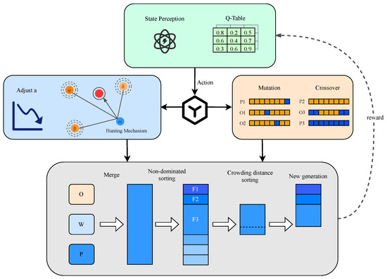
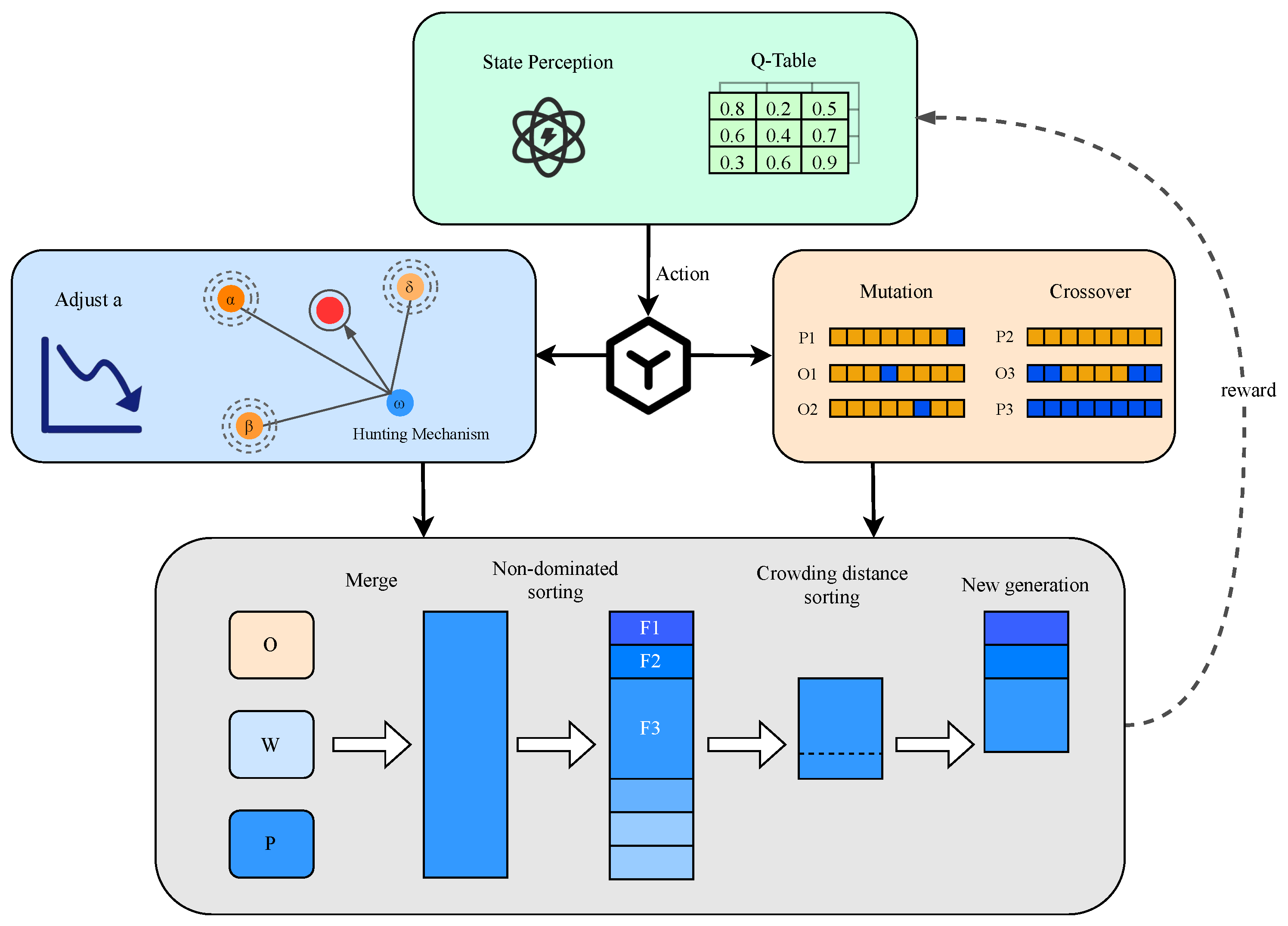
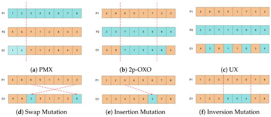
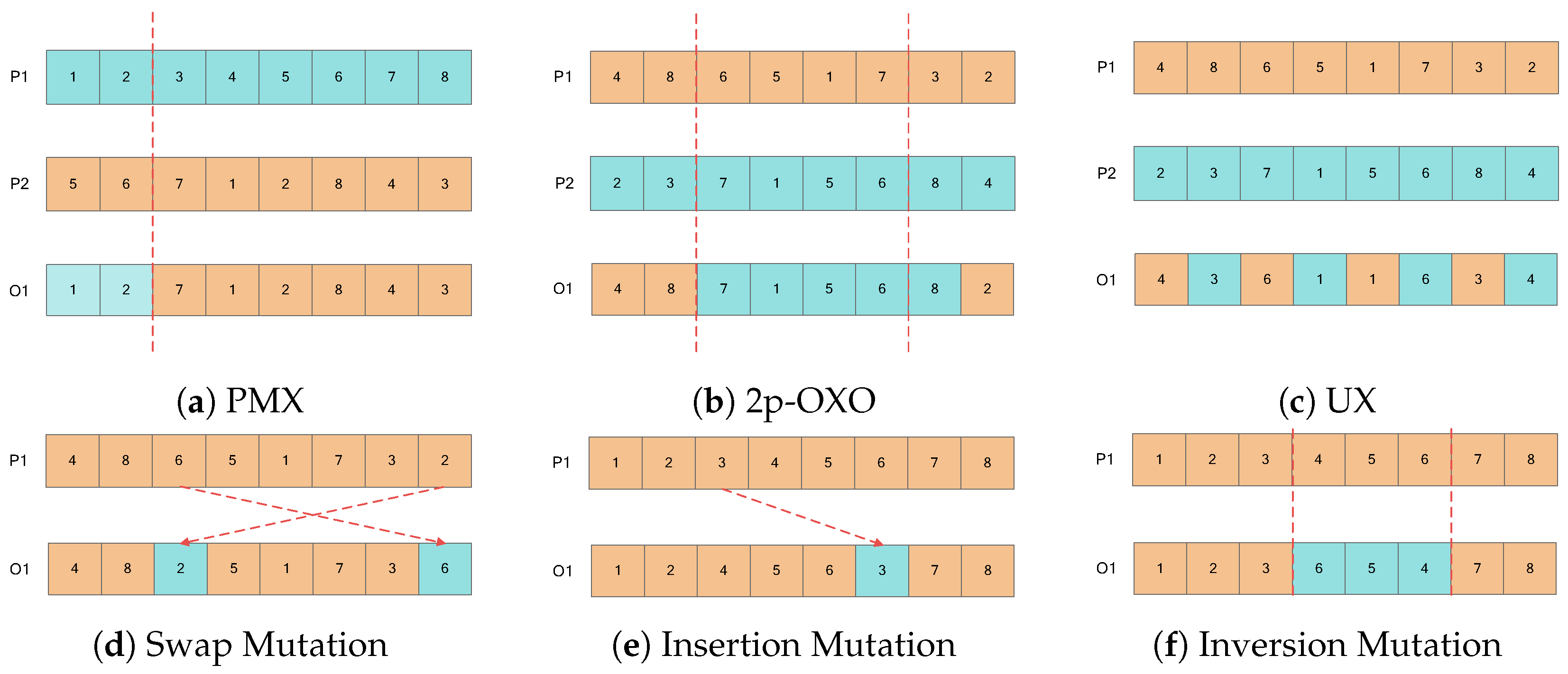
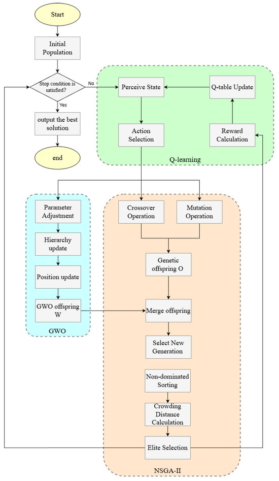
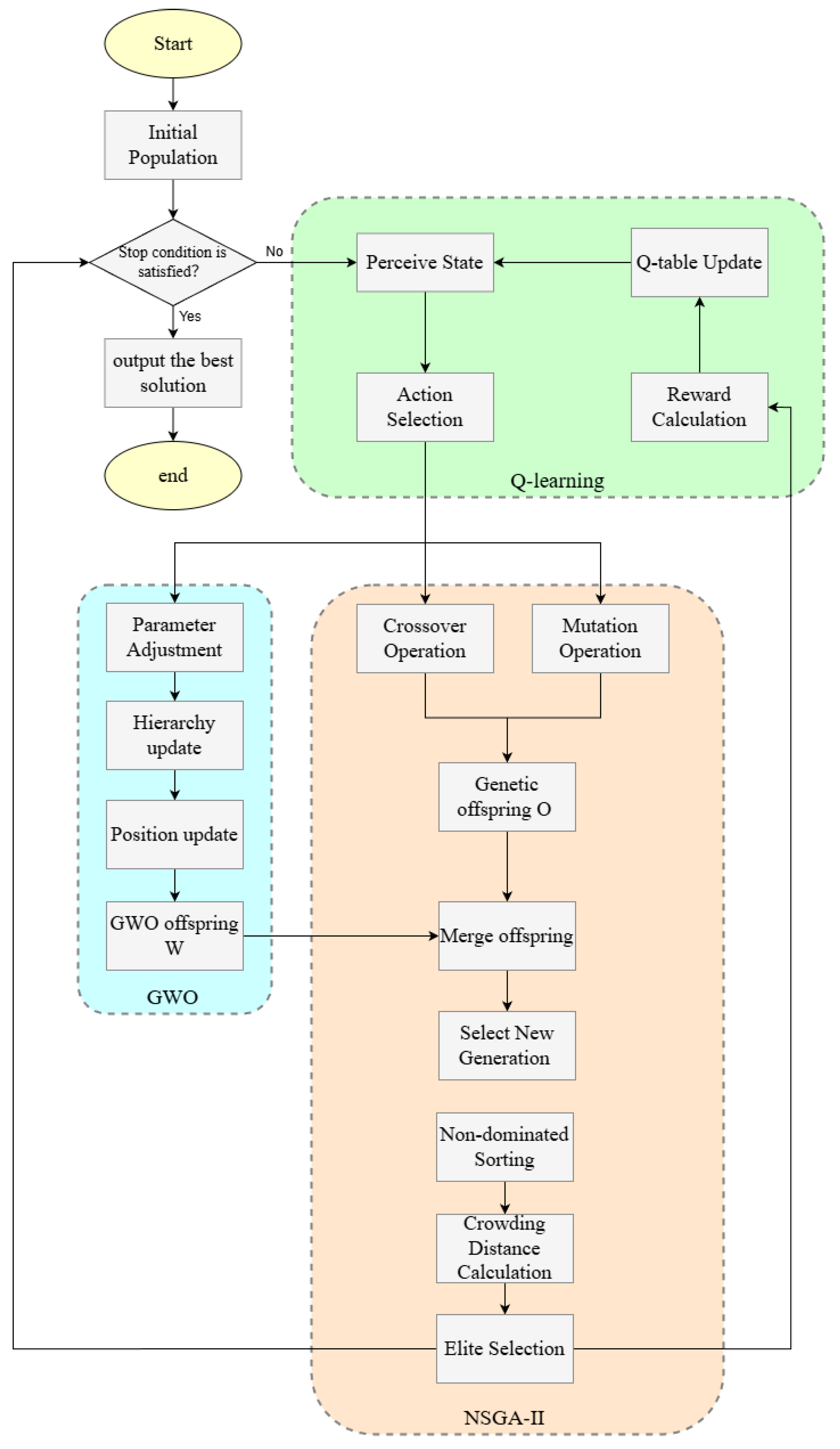
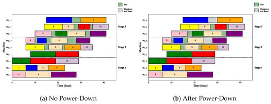
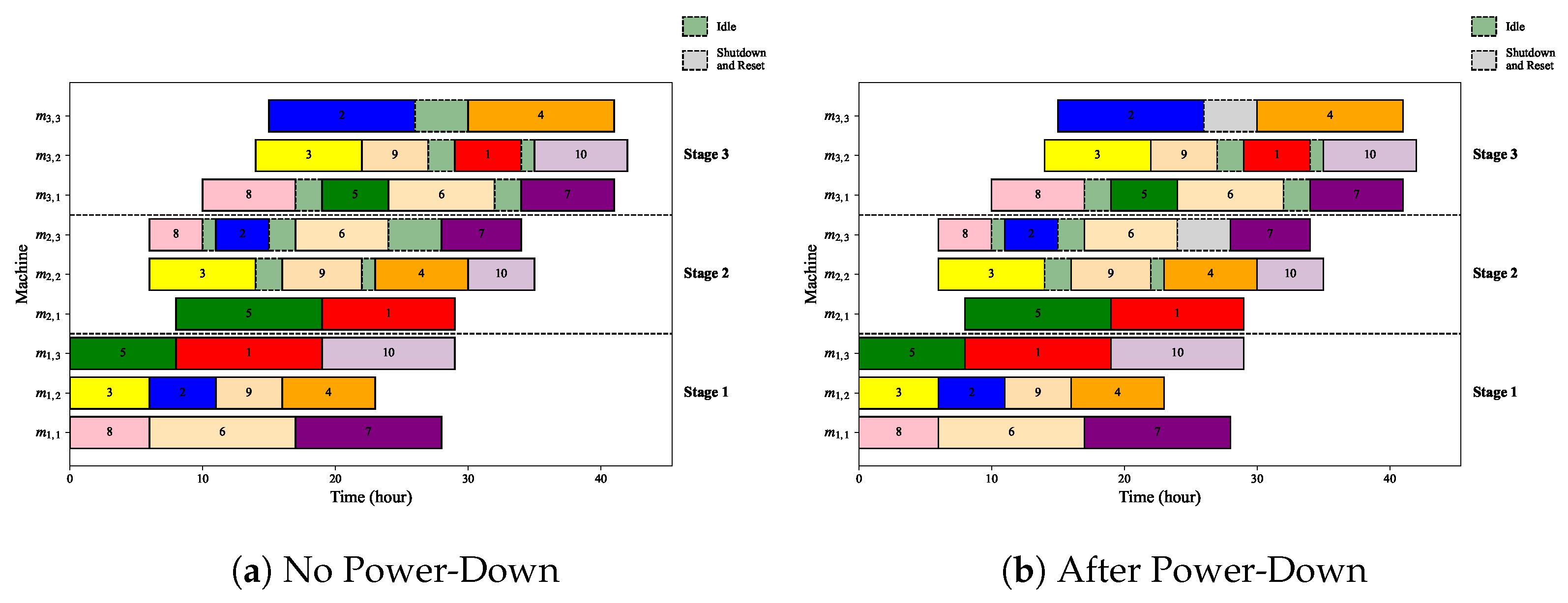
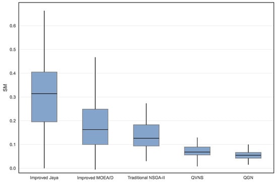
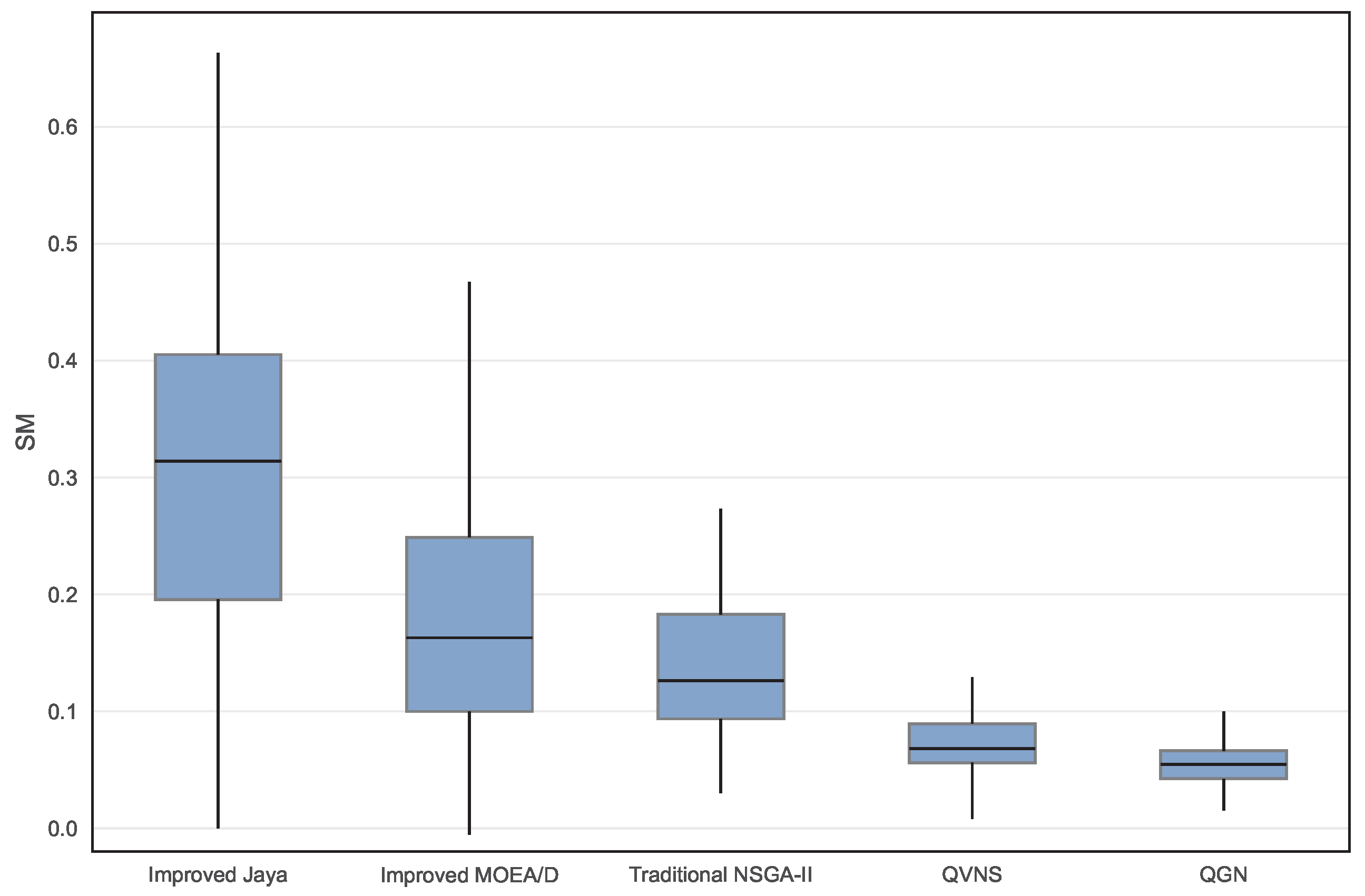

Disclaimer/Publisher’s Note: The statements, opinions and data contained in all publications are solely those of the individual author(s) and contributor(s) and not of MDPI and/or the editor(s). MDPI and/or the editor(s) disclaim responsibility for any injury to people or property resulting from any ideas, methods, instructions or products referred to in the content. |
© 2026 by the authors. Licensee MDPI, Basel, Switzerland. This article is an open access article distributed under the terms and conditions of the Creative Commons Attribution (CC BY) license.