Distributed Stochastic Extremum Seeking for Optimal Resource Allocation over Networks with Time Delays

Abstract

This paper investigates optimal resource allocation in multi-agent networks subject to simultaneous measurement and communication delays. We propose a distributed stochastic extremum seeking (SES) algorithm for connected undirected graphs with heterogeneous constant communication delays. The algorithm uses only delayed pointwise measurements of the local objective values; neither gradient nor Hessian information is fed to the controller. It combines a proportional–integral (PI) consensus protocol, which enforces the supply–demand balance, with a one-stage sequential predictor that compensates for the measurement delays. The convergence analysis is developed for local objectives of quadratic type; this restriction, which is required by the stochastic-averaging argument, is stated explicitly and discussed. Using stochastic averaging theory and Lyapunov–Krasovskii functionals for delay systems, we prove that, for every finite initial history, the estimates converge almost surely to an arbitrarily small neighborhood of the optimum for every fixed tolerance, and we derive an explicit admissible range for the constant communication delays together with a sequential procedure for selecting the design parameters. Two case studies, namely a three-generator microgrid and a six-generator microgrid, are used to illustrate the theoretical results.

1. Introduction

Optimal resource allocation, that is, minimizing the sum of local objectives subject to a coupling constraint, plays a fundamental role in power systems [1], transportation [2], communication networks [3], and supply chain management [4]. In large-scale networks, centralized methods that rely on a single decision maker suffer from drawbacks such as high computational complexity, communication overhead, privacy issues, and single-point failure [5]. Consequently, distributed algorithms, in which each agent keeps a local decision and a local objective and coordinates through limited communication, have therefore been studied extensively (see the survey [6]).

For problems with only equality constraints, existing techniques include interior-point [7], continuous-time designs for balanced digraphs [8], Laplacian eigenvector estimation for unbalanced graphs [9,10], passivity-based approaches for time-varying digraphs [11] and saddle-point/consensus [12]. When both equality and local constraints are present, techniques employ nonsmooth penalties [13,14], projections [9,15,16,17,18], or Lagrange multipliers [19], solved via subgradient [9,13,15], gradient [16], deterministic extremum seeking [14], or primal-dual [19] methods. Most works consider undirected or balanced networks; [18] addresses unbalanced digraphs, and extensions handle time-varying constraints [20] and coupled inequalities [21]. However, these works assume instantaneous, perfect communication. Delays are ubiquitous and can destabilize the system.

Only a few studies incorporate delays: a discrete-time method with homogeneous constant delays [22], an empirical analysis [23], gradient-based methods for heterogeneous constant delays [24] and bounded time-varying delays [25], and a primal-dual stochastic gradient method for heterogeneous time-varying delays on digraphs [26]. Among them, [24,25,26] provide rigorous delay bounds, but they all require gradient information. This requirement becomes restrictive when the objectives are unknown or gradients are costly to obtain [27]. The gradient can instead be estimated from function measurements and exploration signals, which is the principle of extremum seeking (ES); but the classical deterministic scheme relies on phase-aligned periodic dithers [28], and delayed communication destroys that alignment.

Stochastic extremum seeking (SES) removes this difficulty by replacing the periodic dithers with ergodic stochastic exploration, which requires neither orthogonality nor phase coordination and tolerates noisy, delay-affected channels [29,30,31]. The existing SES results for delayed systems, however, do not cover the present setting: those of [30,31] concern a single plant, with no network, no consensus mechanism, and no coupled balance constraint, and the companion work [32] enforces a consensus constraint $x_1=\cdots =x_N$ rather than a supply–demand balance. Consequently, to date, no delay-aware, gradient-free distributed allocation scheme with an explicit admissible delay bound has been available for this setting. Table 1 compares the present scheme with the closest alternatives along five axes: whether gradient information is required; whether measurement delay is modeled; whether communication delay is modeled; whether a heterogeneous delay profile is admitted; and whether an explicit admissible delay bound is provided.

Table 1. Comparison with closely related distributed resource-allocation and extremum-seeking schemes.

Scheme	Gradient Required	Measurement Delay	Communication Delay	Heterogeneous Delays	Explicit Delay Bound
[24]	Yes	No	Yes (constant)	Yes	Yes
[25]	Yes	No	Yes (time-varying)	Yes	Yes
[26]	Yes	No	Yes (time-varying, digraph)	Yes	Yes
[14,15] (deterministic ES)	No	No	No	No	No
[30,31] (SES, single plant)	No	Yes (single plant)	No	Yes	Yes
[32] (companion work)	No	Yes	Yes	Yes	Yes (consensus constraint)
This paper	No	Yes	Yes (constant)	Yes	Yes (balance constraint)

This paper treats two delay channels jointly. The first is the measurement delay, which arises in the sensing and actuation path of an agent: the local cost is evaluated from a signal, such as a meter reading, a price feed, or a state estimate, that reaches the controller only after a processing lag. In an economic-dispatch setting, for instance, the marginal cost of a generator is computed from a state estimate obtained from measurements that may be several hundred milliseconds old [24]. The second is the communication delay, which arises in the network path from a sending agent to a receiving agent, where the exchange of dual variables over a communication link incurs a propagation and queueing delay; in wide-area microgrid control, this delay is on the order of hundreds of milliseconds and is heterogeneous across links. The two channels have different physical origins and different effects on the closed loop, and neither can be absorbed into the other, so both are retained. They also call for different treatments because correlating the delayed objective value with the current exploration phase biases the gradient estimate; it is therefore compensated actively by a one-stage sequential predictor that reconstructs the current demodulated value. The communication delay instead acts on the consensus dynamics, reducing the stability margin of the loop; it is accommodated rather than compensated, by deriving an admissible upper bound on its magnitude within which convergence is guaranteed. The two treatments are complementary rather than interchangeable: compensating the measurement delay alone still leaves the consensus dynamics subject to the communication delay, while the bound alone does not remove the bias of the gradient estimate.

The main contributions of this paper are fourfold. First, we propose a distributed SES algorithm that handles measurement and heterogeneous constant communication delays simultaneously, under a supply–demand balance constraint, using only delayed measurements of the local objective functions; neither gradient nor Hessian information is fed to the controller. Second, the algorithm embeds a proportional–integral (PI) consensus mechanism whose integral channel enforces the global supply–demand balance, and the equilibrium analysis identifies the PI-consensus equilibria with the Karush–Kuhn–Tucker (KKT) points of the allocation problem (Lemma 1). Third, we derive an explicit admissible delay bound for constant communication delays from four scalar inequalities (Theorem 1), together with a sequential procedure for selecting the design parameters (Section 3.2). Fourth, the analysis rests on a Lyapunov–Krasovskii construction for the resulting multi-delay averaged system (Appendix A), used together with a stochastic averaging theorem for multiple delays whose hypotheses are verified for the present problem (Appendix B). In the delay-free limit, the scheme reduces to the known distributed ES/PI-consensus designs [14,15], and no novelty is claimed for that special case; relative to [32], the balance constraint enforced by the PI loop, whose integrator acts as the KKT multiplier, alters the equilibrium analysis (Lemma 1 rather than a consensus manifold) and adds a further block to the Lyapunov analysis.

The remainder of this paper is organized as follows. Section 2 formulates the problem and states the standing assumptions. Section 3 presents the proposed algorithm and its convergence analysis. Section 4 reports simulation results, and Section 5 concludes with limitations and future directions.

2. Preliminaries and Problem Formulation

2.1. Notations and Graph Theory

${\parallel A\parallel }_2$ denotes the spectral norm of matrix A, and $\parallel x\parallel$ denotes the Euclidean norm of vector x. $I_n$ is the $n\times n$ identity matrix; ${\mathbf{1}}_n$, ${\mathbf{0}}_n$ are the n-dimensional vectors of ones and zeros, respectively. ${\lambda }_{\max }\left(A\right)$ and ${\lambda }_{\min }\left(A\right)$ denote the largest and smallest eigenvalues of a square matrix A. $A\otimes B$ is the Kronecker product. For a ${\mathcal{C}}^1$ function $g{:}^n\to$, $\nabla g$ is its gradient. Throughout, a function of a vector argument, such as $\sin (·)$, is applied componentwise.

For $\tau >0$, let ${𝒞}_n^{\tau }:=\mathcal{C}([-\tau ,0],{\mathbb{R}}^n)$ denote the Banach space of continuous functions mapping $[-\tau ,0]$ to ${\mathbb{R}}^n$, equipped with the norm $\parallel \phi \parallel ={\sup }_{\theta \in [-\tau ,0]}\left|\phi \left(\theta \right)\right|$. The prescribed history function of agent i is written ${\phi }_i\in C_n^{{\tau }^{*}}$, with ${\tau }^{*}$ the maximum delay introduced in Section 3.1. This notation resolves the subscript–superscript pair: ${𝒞}_n^{\tau }$ is the space of ${\mathbb{R}}^n$-valued continuous functions on an interval of length $\tau$.

The communication topology of an N-agent network is an undirected graph $\mathcal{G}=(\mathcal{V},\mathcal{E})$ with $\mathcal{V}=\{1,\dots ,N\}$. The adjacency matrix $A=\left[a_{ij}\right]\in {\mathbb{R}}^{N\times N}$ is symmetric and satisfies $a_{ij}=a_{ji}>0$ if and only if $(j,i)\in \mathcal{E}$, and $a_{ii}=0$ (no self-loops). The neighbor set of agent i is ${\mathcal{N}}_i=\{j\mid (j,i)\in \mathcal{E}\}$. The Laplacian matrix $\mathcal{L}=\left[l_{ij}\right]{\in }^{N\times N}$ is defined by $l_{ii}={\sum }_{j\ne i}{a}_{ij}$ and $l_{ij}=-a_{ij}$ for $i\ne j$. If $\mathcal{G}$ is connected, $\mathcal{L}$ is symmetric positive semidefinite with a simple zero eigenvalue and associated eigenvector ${\mathbf{1}}_N$; a systematic treatment of consensus dynamics built on this spectrum is given in [33]. Its eigenvalues satisfy

$$0={\lambda }_1<{\lambda }_2\le \cdots \le {\lambda }_N.$$

(1)

We emphasize that, whenever a quantity is denoted ${\lambda }_2$ in this paper, it denotes the smallest positive eigenvalue of the Laplacian.

2.2. Resource Allocation Problem Description

Each agent $i\in \mathcal{V}$ has a local objective $f_i:{\mathbb{R}}^n\to \mathbb{R}$ that is not available in explicit form and can only obtain its measurements. The agents cooperatively solve

$$\begin{array}{cc}\hfill \underset{\mathbf{x}\in {\mathbb{R}}^{nN}}{\min }f\left(\mathbf{x}\right)& ={\displaystyle \sum _{i=1}^N}{f}_i\left(x_i\right),\mathrm{s}.\mathrm{t}.{\displaystyle \sum _{i=1}^N}{x}_i={\displaystyle \sum _{i=1}^N}{d}_i,\hfill \end{array}$$

(2)

where $\mathbf{x}=\mathrm{col}(x_1,\dots ,x_N)\in {\mathbb{R}}^{nN}$ with the supply $x_i\in {\mathbb{R}}^n$ and the known demand $d_i\in {\mathbb{R}}^n$ of agent i; the equality constraint ensures global supply–demand balance.

Assumption 1. 

Problem (2) is feasible: there exists $x=\mathrm{col}(x_1,\dots ,x_N)\in {\mathbb{R}}^{nN}$ with ${\sum }_i{x}_i={\sum }_i{d}_i$, and the infimum in (2) is finite.

Assumption 2. 

Each $f_i$ is twice continuously differentiable and ${\mathsf{\ell }}_i$-strongly convex with ${\mathsf{\ell }}_i$ > 0.

No Slater-type strict-feasibility condition is imposed. Since the only constraint in (2) is an affine equality constraint, the constraint qualification holds automatically whenever the feasible set is nonempty, so such a condition would be vacuous here. The essential requirement is feasibility together with finiteness of the optimal value, which is what Assumption 1 asserts. Under Assumptions 1 and 2, Problem (2) admits a unique optimal solution ${\mathbf{x}}^{*}=\mathrm{col}(x_1^{*},\dots ,x_N^{*})$. By the first-order optimality condition, there exists $\overline{\lambda }\in {\mathbb{R}}^n$ such that $\nabla f_i\left(x_i^{*}\right)=\overline{\lambda }$ for all $i\in \mathcal{V}$ and ${\sum }_i{x}_i^{*}={\sum }_i{d}_i$.

Time delays are inherent in practical communication and measurement processes. Let ${\tau }_{c_{ij}}>0$ be the constant communication delay from agent j to agent i, $j\in {\mathcal{N}}_i$, and ${\tau }_{m_i}>0$ be the measurement delay of agent i, known to agent i. Hence, agent i only receives delayed neighbor information and its own delayed measurements, with respective delays ${\tau }_{c_{ij}}$ and ${\tau }_{m_i}$.

Assumption 3. 

The undirected graph $\mathcal{G}$ is connected, and ${\tau }_{c_{ij}}={\tau }_{c_{ji}}>0$ for every $(j,i)\in \mathcal{E}$.

Remark 1. 

Assumption 3 imposes two restrictions: connectivity of the undirected graph, and symmetric constant delays ${\tau }_{c_{ij}}={\tau }_{c_{ji}}$ on every edge, which corresponds to a bidirectional physical link with identical propagation delays in both directions. Both are standard in undirected consensus problems [24]. They are also genuine limitations of the present analysis, and we state them explicitly. (i) The symmetry ${\tau }_{c_{ij}}={\tau }_{c_{ji}}$ is used in the decomposition ${\sum }_{p=1}^{N_0}{\mathcal{L}}^{\left(p\right)}=\mathcal{L}$ with symmetric ${\mathcal{L}}^{\left(p\right)}$, and therefore in the spectral argument of the convergence analysis in Section 3.2. Asymmetric delays destroy this symmetry and require substantially different tools. (ii) The delay bound of Theorem 1 is derived for constant delays. Time-varying delays would require the Lyapunov–Krasovskii functional to be augmented by terms that bound the delay derivative, and the resulting admissible bound is generally smaller and depends on the delay rate. (iii) The Laplacian enters the delay bound through the quantities ${\lambda }_2$ and ${\parallel \mathcal{L}\parallel }_2$ in the coefficient ${\varsigma }_3$ of Theorem 1; the dependence on network connectivity is discussed in Section 3.2. Extensions to directed, switching, or disconnected topologies, and to asymmetric, time-varying, or stochastic delays, are identified as future work.

The first-order necessary condition for problem (2) is recalled as follows.

Lemma 1. 

Let each $f_i$ be $C^1$ and convex, let the feasible set of (2) be nonempty, and let $x_i^{*}{\in }^n$, $i\in \mathcal{V}$, be a minimizer of (2). Then, there exists $\overline{\lambda }{\in }^n$ such that

$$-\nabla f_i\left(x_i^{*}\right)+\overline{\lambda }=0,\sum _{i\in \mathcal{V}}{x}_i^{*}=\sum _{i\in \mathcal{V}}{d}_i,$$

(3)

holds for all $i\in \mathcal{V}$. Conversely, any feasible $x_i^{*}\in {\mathbb{R}}^n$, $i\in \mathcal{V}$, and $\overline{\lambda }\in {\mathbb{R}}^n$ satisfying (3) give a global optimum.

Proof. 

The feasible set $\{x:{\sum }_i{x}_i={\sum }_i{d}_i\}$ is an affine subspace, hence convex; by Assumption 1 it is nonempty. Since all equality constraints are affine, the KKT constraint qualification holds automatically ([34], Section 5.5.3), so the KKT conditions are necessary for optimality; under convexity of the $f_i$ they are also sufficient ([34], Section 5.5.3). With the Lagrangian $L(x,\overline{\lambda })={\sum }_i{f}_i\left(x_i\right)+{\overline{\lambda }}^T\left({\sum }_i{d}_i-{\sum }_i{x}_i\right)$, one has ${\nabla }_{x_i}L=\nabla f_i\left(x_i\right)-\overline{\lambda }$, and the stationarity and feasibility conditions of the KKT system reduce to (3). Both directions follow. □

3. Algorithm Design and Convergence Analysis

Consensus-based coupling terms enforce the supply–demand balance, and stochastic extremum seeking approximates local gradients, removing the need for explicit gradient information.

3.1. Algorithm Design

Let the maximum measurement and communication delays be

$$\begin{array}{c}\hfill {\tau }_m^{*}=\underset{i\in \mathcal{V}}{\max }\left\{{\tau }_{m_i}\right\},{\tau }_c^{*}=\underset{(i,j)\in \mathcal{E}}{\max }\left\{{\tau }_{c_{ij}}\right\},\end{array}$$

and let the maximum delay be ${\tau }^{*}=\max \{{\tau }_m,{\tau }_c\}$. Let the delayed objective be ${\tilde{f}}_i\left(t\right)=f_i\left(x_i(t-{\tau }_{m_i})\right)$. For agent i and $t\ge 0$, the proposed distributed stochastic extremum seeking algorithm is

$$\begin{array}{cc}\hfill x_i\left(t\right)& ={\widehat{x}}_i\left(t\right)+b_i\sin \left({\eta }_i(t+{\tau }_{m_i})\right),\hfill \end{array}$$

(4)

$$\begin{array}{cc}\hfill {\dot{\widehat{x}}}_i\left(t\right)& =\alpha \left\{-{\xi }_i\left(t\right)+{\mu }_i\left(t\right)\right\},\hfill \end{array}$$

(5)

$$\begin{array}{cc}\hfill {\dot{\xi }}_i\left(t\right)& =\alpha N_i\left(t\right){\tilde{f}}_i\left(t\right)\left\{-{\xi }_i\left(t\right)+{\mu }_i\left(t\right)\}+\beta \{M_i\left(t\right){\tilde{f}}_i\left(t\right)-{\xi }_i(t-{\tau }_{m_i})\right\},\hfill \end{array}$$

(6)

$$\begin{array}{cc}\hfill {\dot{\mu }}_i\left(t\right)& =-\gamma \sum _{j\in {\mathcal{N}}_i}{a}_{ij}\left({\mu }_i(t-{\tau }_{c_{ij}})-{\mu }_j(t-{\tau }_{c_{ij}})\right)-\alpha z_i\left(t\right)+\alpha \left(d_i-{\widehat{x}}_i\left(t\right)\right),\hfill \end{array}$$

(7)

$$\begin{array}{cc}\hfill {\dot{z}}_i\left(t\right)& =\gamma \sum _{j\in {\mathcal{N}}_i}{a}_{ij}\left({\mu }_i(t-{\tau }_{c_{ij}})-{\mu }_j(t-{\tau }_{c_{ij}})\right),\hfill \end{array}$$

(8)

where ${\widehat{x}}_i\left(t\right)$ is the estimate of the optimal allocation $x_i^{*}$; $b_i=(b_{i1},\dots ,$$b_{in})$ is the exploration amplitude matrix; $\alpha ,\beta ,\gamma >0$ are design parameters; ${\xi }_i\left(t\right)$ compensates the measurement delay ${\tau }_{m_i}$ (a one-stage sequential predictor); and ${\mu }_i\left(t\right)$, $z_i\left(t\right)$ are the proportional–integral (PI) consensus terms, with $z_i\left(t\right)$ integrating the consensus error. The sine function in (4) is understood componentwise for vector arguments, i.e., $\sin \left({\eta }_i(t+{\tau }_{m_i})\right)=(\sin \left({\eta }_{i1}(t+{\tau }_{m_i})\right),\dots ,\sin \left({\eta }_{in}(t+{\tau }_{m_i})\right))$. The stochastic exploration signal ${\eta }_i\left(t\right)=({\eta }_{i1}\left(t\right),\dots ,{\eta }_{in}\left(t\right))$ has independent components evolving according to the process

$$\begin{array}{c}\hfill \epsilon \mathrm{d}{\eta }_{ij}\left(t\right)=-{\eta }_{ij}\left(t\right)\mathrm{d}t+\sqrt{\epsilon }{q}_{ij}\mathrm{d}{W}_{ij}\left(t\right),\end{array}$$

(9)

in which $\epsilon \in (0,{\epsilon }_0)$ controls the exploration timescale, $q_{ij}>0$ scales the noise intensity, and $W_{ij}\left(t\right)$ are mutually independent standard Wiener processes. In (6), $N_i\left(t\right)={\left[N_i^{jk}\left(t\right)\right]}_{j,k=1}^n\in {\mathbb{R}}^{n\times n}$ and $M_i\left(t\right)\in {\mathbb{R}}^n$ are given by

$$\begin{array}{cc}\hfill M_i\left(t\right)& ={\left[{\displaystyle \frac{\sin \left({\eta }_{i1}\left(t\right)\right)}{b_{i1}{G}_0\left(q_{i1}\right)}},{\displaystyle \frac{\sin \left({\eta }_{i2}\left(t\right)\right)}{b_{i2}{G}_0\left(q_{i2}\right)}},\dots ,{\displaystyle \frac{\sin \left({\eta }_{iN}\left(t\right)\right)}{b_{in}{G}_0\left(q_{in}\right)}}\right]}^T,\hfill \\ \hfill N_i^{jk}\left(t\right)& =\left\{\begin{array}{cc}{\displaystyle \frac{4({\sin }^2\left({\eta }_{ij}\left(t\right)\right)-G_0\left(q_{ij}\right))}{b_{ij}^2{G}_0^2\left(\sqrt{2}{q}_{ij}\right)}},& j=k,\\ {\displaystyle \frac{\sin \left({\eta }_{ij}\left(t\right)\right)\sin \left({\eta }_{ik}\left(t\right)\right)}{b_{ij}{b}_{ik}{G}_0\left(q_{ij}\right)G_0\left(q_{ik}\right)}},& j\ne k,\end{array}\right.\hfill \end{array}$$

with $G_0\left(q_{ij}\right)={\displaystyle \frac{1}{2}}(1-\exp \{-q_{ij}^2\})$.

The initial conditions for algorithm (4)–(8) are prescribed as follows. For all $t\in [-{\tau }^{*},0]$, ${\widehat{x}}_i\left(t\right)={\widehat{x}}_i\left(0\right)=x_i\left(0\right)$, where ${\widehat{x}}_i\left(0\right)\in {\mathbb{R}}^n$ denotes the initial estimate of agent i. ${\xi }_i\left(t\right)$=${\phi }_i\in {𝒞}_n^{{\tau }^{*}}$ is the prescribed initial function of the predictor; ${\mu }_i(·)\in {𝒞}_n^{{\tau }^{*}}$ is chosen as the constant extension and ${\mu }_i\left(t\right)={\mu }_i\left(0\right)$ on $[-{\tau }^{*},0]$. The initial values ${\mu }_i\left(0\right),z_i\left(0\right)\in {\mathbb{R}}^n$ are assumed to be finite.

Equation (4) applies the exploration signal at the shifted argument $t+{\tau }_{m_i}$. Because the plant state and the plant noise do not enter the generation of ${\eta }_i$, this shift requires no future plant increments and is realizable causally. To make the construction explicit, enlarge the probability space so that $\left\{W_{ij}\right\}$ is a two-sided Wiener process defined for $t\in \mathbb{R}$, independent of the Wiener processes driving any other stochastic component of the plant, and let ${\mathcal{F}}_t^{\eta }=\sigma \{W_{ij}\left(s\right):s\le t,i\in \mathcal{V},j\in \{1,\dots ,n\}\}$ be the filtration it generates; then ${\eta }_{ij}$ defined by (9) from the stationary law is stationary and ergodic, and ${\eta }_{ij}(t+{\tau }_{m_i})$ is measurable with respect to ${\mathcal{F}}_{t+{\tau }_{m_i}}^{\eta }$. In an implementation the simulator of (9) runs on a fast clock advanced by ${\tau }_{m_i}$ ahead of the plant clock, so the value fed to (4) at time t is the value the plant-independent simulator has already produced for $t+{\tau }_{m_i}$; since ${\tau }_{m_i}$ is finite and known, this advance is realized by buffering a horizon of length ${\tau }_{m_i}$ of the simulated path, or equivalently by prescribing a realization of the ergodic exploration path over the whole control horizon in advance. In either case, the shifted signal is a prescribed, ergodic, exogenous input, so the hypotheses required by the averaging argument, namely ergodicity and independence from the initial state, are preserved. The shift makes the delayed measurement ${\tilde{f}}_i\left(t\right)=f_i({\widehat{x}}_i(t-{\tau }_{m_i})+b_i\sin \left({\eta }_i\left(t\right)\right))$ correlate with the current exploration phase appearing in $M_i\left(t\right)$ and $N_i\left(t\right)$; at the level of the slow system it cancels against the measurement delay, so no future increment of the state enters the averaged dynamics (Appendix B.3.2).

To make the measurement-delay compensation explicit, the predictor ${\xi }_i$ in (5) and (6) is interpreted as follows. Absent delay, the averaged extremum-seeking loop updates the estimate along the demodulated gradient; the demodulated quantity available at time t is built, however, from the measurement ${\tilde{f}}_i\left(t\right)=f_i\left(x_i(t-{\tau }_{m_i})\right)$, that is, from the state at the earlier time $t-{\tau }_{m_i}$. Using it directly in (5) would act on a stale gradient, with a bias of order ${\tau }_{m_i}$ times the gradient’s rate of change. The predictor ${\xi }_i$ instead stores a running model-driven estimate of $\alpha (-{\xi }_i+{\mu }_i)$ and drives it toward the delayed measurement through the term $-{\xi }_i(t-{\tau }_{m_i})$ in (6); a single prediction step over the known, constant horizon ${\tau }_{m_i}$ suffices, which is why it is called one-stage. In the averaged error system, this mechanism appears as the error variable $\zeta =H{\widehat{\mathbf{x}}}^a+c-{\xi }^a$, which evolves as a benign delayed linear filter $\dot{\zeta }\left(t\right)=-\beta \zeta (t-{\tau }_m)$: the measurement-delay error decays to zero instead of corrupting the gradient estimate, the decay being guaranteed by the measurement-delay condition of Theorem 1.

The PI consensus plays two distinct roles. The proportional channel $\gamma {\sum }_{j\in {\mathcal{N}}_i}{a}_{ij}({\mu }_i-{\mu }_j)$ in (7) and (8) is the standard consensus coupling on the dual variables, driving ${\mu }_i$ toward agreement across the network, whereas the integral channel $z_i$ is what enforces the balance constraint. Summing (8) over i and using ${\mathbf{1}}_N^T\mathcal{L}=0$ gives ${\sum }_i{\dot{z}}_i\left(t\right)=0$, so ${\sum }_i{z}_i\left(t\right)={\sum }_i{z}_i\left(0\right)$; with the initialization ${\sum }_i{z}_i\left(0\right)=0$ this propagates for all time. At equilibrium, it yields ${\mathbf{z}}_{eq}=d-{\mathbf{x}}^{*}$ and then ${\sum }_i{x}_{eq,i}={\sum }_i{d}_i$, i.e., exact supply–demand balance: the integral term drives the total mismatch to zero, while the proportional term governs the transient agreement of the multipliers. Without the integral channel, the equilibrium would enforce only consensus of the multipliers and could not satisfy the resource balance. The equilibrium ${\mu }_{eq}={\mathbf{1}}_N\otimes \overline{\lambda }$ identifies $\mu$ with the Lagrange multiplier of (2), so the PI loop simultaneously recovers the KKT multiplier and enforces feasibility.

The exploration is stochastic rather than deterministic. Deterministic extremum seeking employs periodic sinusoids whose orthogonality is needed to decouple the gradient estimates for the n inputs of each agent and across the network, and this requires exact phase synchronization; communication and measurement delays destroy that alignment and make coordinated orthogonal dither scheduling impractical in large networks. Stochastic exploration (9) is ergodic and needs neither orthogonality nor phase coordination, with its gradient and Hessian estimates following from ergodic correlations [29,30,31]. Three considerations govern the choice of its parameters. (i) Timescale separation: $\epsilon$ sets the ratio of the exploration timescale to the allocation timescale and is chosen so that the correlation time $O\left(\epsilon \right)$ is at least an order of magnitude shorter than the slowest closed-loop mode, the residual bias of the averaged system being of order $O\left(\epsilon \right)$. (ii) Noise intensity: $q_{ij}$ controls the excursion amplitude; the demodulation gains are normalized by $G_0\left(q_{ij}\right)=\frac{1}{2}(1-e^{-q_{ij}^2})$, the stationary mean of ${\sin }^2\left({\eta }_{ij}\right)$, which makes the gradient estimate consistent for any $q_{ij}>0$, so $q_{ij}$ is a conditioning rather than a tuning parameter. A sufficiently small $q_{ij}$ inflates the demodulation gain, while a sufficiently large one saturates the sinusoid and wastes excitation energy. (iii) Amplitude trade-off: larger $b_{ij}$ improve the gradient signal-to-noise ratio but enlarge the ultimate neighborhood of the optimum, since the dither-induced residual of $\mathbf{x}\left(t\right)$ around ${\mathbf{x}}^{*}$ is of order $\parallel b\parallel$ (Remark 3); the amplitudes are therefore chosen as the smallest values giving an acceptable gradient estimate, a standard bias–variance compromise [28].

3.2. Convergence Analysis

For any twice continuously differentiable and strongly convex function $f_i\left(x\right)$, the Hessian matrix at the optimum $x^{*}$ is positive definite. Performing a second-order Taylor expansion of $f_i\left(x\right)$ around $x_i^{*}$ therefore yields a quadratic approximation. Hence, we adopt the following assumption.

Assumption 4. 

Each local objective function $f_i$ in (2) is quadratic:

$$f_i\left(x_i\right)={\displaystyle \frac{1}{2}}{x}_i^T{H}_i{x}_i+c_i^T{x}_i+s_i,i\in \mathcal{V},$$

(10)

with positive definite $H_i=H_i^T{\in }^{n\times n}$.

Remark 2. 

Assumption 2 is a problem-level requirement, since strong convexity ensures uniqueness of the optimum; Assumption 4 is the working hypothesis for the convergence analysis and is a real restriction. Under Assumption 4, the gradient is $\nabla f_i\left(x_i\right)=H_i{x}_i+c_i$, so the gradient is determined by the parameters $H_i$ and $c_i$. This is why the design is not described here as “gradient-free” in an absolute sense: what the algorithm avoids is the need for gradient measurements and for analytic knowledge of the gradient map. It uses only delayed pointwise values of $f_i$, and the coefficients $H_i,c_i$ need not be known to the controller, as the demodulation in (6) estimates the gradient from these measurements alone. The restriction to Assumption 4 is nevertheless genuine, and it is imposed by the analysis rather than by the algorithm. Operationally, the algorithm is model-free: it consumes only delayed pointwise values of $f_i$ and would run unchanged for a nonquadratic objective, the quadratic hypothesis being required by the proof rather than by the controller. The setting is relevant when the marginal-cost parameters $H_i,c_i$ are unknown a priori; if they were known, problem (2) would reduce to a linear system solvable without learning.

We specify the scope of the claim as follows. A general twice continuously differentiable strongly convex $f_i$ lies outside the present analysis. Take $f_i\left(x_i\right)=\frac{1}{2}\parallel x_i{\parallel }^2+a{\parallel x_i\parallel }^4$ with $a>0$: it is smooth, strongly convex and minimized at the origin, yet the Taylor remainder about a point $x_i$ is $a\parallel x_i{\parallel }^4$, which does not become $O(\parallel b{\parallel }^3)$ as $\parallel b\parallel \to 0$ for fixed nonzero $x_i$. The higher-order terms therefore cannot be absorbed merely by shrinking the exploration amplitude. Concluding that they are harmless would require a local invariance argument showing that the trajectories remain in an $O(\parallel b\parallel )$ neighborhood of the optimum, together with uniform regularity and perturbation estimates for the averaged system; $C^2$ regularity alone does not yield a cubic remainder. No such argument is pursued here, and the Abstract, Theorem 1 and the Conclusion are accordingly restricted to quadratic objectives. Extending Theorem 1 to general strongly convex objectives, either by a rigorous two-time-scale perturbation analysis or by a different Lyapunov construction, is left open. The restriction enters at a single point: the averaging argument of ([32], Theorem 4.7) requires the origin of the averaged system to be locally exponentially stable, and we establish this through the linear averaged error dynamics (37)–(40), which Assumption 4 makes available. Appendix B.5 locates that step.

We next identify the class of nonquadratic objectives to which the analysis could be extended, although no such extension is developed here. Two routes are natural. The first is a vanishing-amplitude scheme, in which the exploration amplitude is decayed rather than held fixed, so that the fixed-amplitude residual that obstructs the argument above could be made to vanish asymptotically, at the price of a slower transient. The second is a higher-order perturbation analysis, in which the averaged error system is analyzed without discarding the higher-order terms of $f_i$ that the quadratic model drops, accompanied by a local invariance argument showing that the averaged trajectories remain in a neighborhood where the quadratic model is accurate. Either route, if carried through, could cover twice continuously differentiable strongly convex objectives with a bounded third derivative. Neither is pursued here; the two routes indicate where the quadratic restriction might be relaxed.

The global well-posedness of the closed loop on the whole half-line, which is Assumption A2 of the averaging framework of Appendix B, is not needed for the conclusion, and it is therefore not imposed as an additional hypothesis of Theorem 1. The framework enters the proof only through its comparison estimate, and that estimate is used on an interval stopped at the first exit of the trajectory from the finite bound of the averaged solution. On every fixed compact interval, the stopped comparison is available for all sufficiently small $\epsilon$, and this is all that (15) requires, because (15) is a statement about the limit $\epsilon \to 0$ and not about any single value of $\epsilon$. The verification is given in Appendix B.3.4.

Theorem 1. 

Under Assumptions 1–4, if $\alpha ,\beta ,\gamma >0$, ${\tau }_c^{*}$, and ${\tau }_m^{*}$ satisfy

$$\begin{array}{cc}\hfill {\varsigma }_1& >0,\hfill \end{array}$$

(11)

$$\begin{array}{cc}\hfill {\varsigma }_2& >0,\hfill \end{array}$$

(12)

$$\begin{array}{cc}\hfill \rho -{\varsigma }_3{\tau }_c^{*2}& >0,\hfill \end{array}$$

(13)

$$\begin{array}{cc}\hfill 1-2\iota N{\beta }^2{\tau }_m^{*2}& >0,\hfill \end{array}$$

(14)

where $H=\mathrm{diag}\left\{H_1,\dots ,H_N\right\}$ and

$$\begin{array}{cc}\hfill {\varsigma }_1& ={\displaystyle \frac{1}{2}}\kappa \left\{\alpha (\kappa +1){\lambda }_{\min }\left(H\right)-\alpha \left(3+{2\parallel H\parallel }_2^2\right)-{\displaystyle \frac{3}{\kappa {\lambda }_2}}\gamma {(\kappa +2)}^2-{\displaystyle \frac{8\rho }{\kappa }}\left({\alpha }^2+{\gamma }^2{\parallel \mathcal{L}\parallel }_2^2\right)\right\},\hfill \\ \hfill {\varsigma }_2& ={\displaystyle \frac{1}{2}}\alpha \kappa -{\displaystyle \frac{1}{2}}{\alpha }^3\kappa (\kappa +1)\left({\parallel H\parallel }_2+1\right)-{\displaystyle \frac{5{\alpha }^4{(\kappa +1)}^4}{4{\kappa }^2}}\gamma -4{\alpha }^2\rho ,\hfill \\ \hfill {\varsigma }_3& ={\displaystyle \frac{\kappa N_0^2{\parallel \mathcal{L}\parallel }_2^2}{2{\lambda }_2^2}}\left\{\alpha {(1-\alpha )}^2{(\kappa +1)}^2+{\lambda }_2^2\gamma \left({\lambda }_2\kappa +2\kappa +2\right)\right\},\hfill \end{array}$$

with $\rho >0$, $\iota >2$, $\kappa >\max \{1,(3+{2\parallel H\parallel }_2^2)/{\lambda }_{\min }\left(H\right)-1\}$; $N_0$ is the number of distinct communication delays. Then there exist $\varpi ,\nu >0$ such that for any initial conditions with $|\widehat{\mathbf{x}}\left(0\right)-{\mathbf{x}}^{*}|<\infty$, $|{\mu }_i\left(0\right)|<\infty$, ${\phi }_i\in {𝒞}_n^{{\tau }^{*}}$, $z_i\left(0\right)\in {\mathbb{R}}^n$ satisfying ${\sum }_{i=1}^N{z}_i\left(0\right)=0$, and any $\delta >0$,

$$\begin{array}{cc}\hfill \underset{\epsilon \to 0}{\lim }\inf \left\{t\ge 0:∥\widehat{\mathbf{x}}\left(t\right)-{\mathbf{x}}^{*}∥>\varpi \psi \left(0\right)\exp \{-\nu t\}+\delta \right\}& =+\infty ,a.s.\hfill \end{array}$$

(15)

where $\widehat{\mathbf{x}}\left(t\right)=\mathrm{col}({\widehat{x}}_1\left(t\right),\dots ,{\widehat{x}}_N\left(t\right))$, $\mathbf{z}\left(0\right)=\mathrm{col}(z_1\left(0\right),\dots ,$$z_N\left(0\right)$, $\phi =\mathrm{col}({\phi }_1,\dots ,{\phi }_N)$, $c=\mathrm{col}(c_1,\dots ,c_N)$, and

$$\begin{array}{cc}\hfill \psi \left(0\right)& =∥\widehat{\mathbf{x}}\left(0\right)-{\mathbf{x}}^{*}∥+\left.∥\mathbf{z}\left(0\right)-(d-{\mathbf{x}}^{*})\right|+{\displaystyle \sum _{i=1}^N}∥{\mu }_i\left(0\right)-{\displaystyle \sum _{i=1}^N}(H_i{x}_i^{*}+c_i)∥\hfill \\ \hfill & +\underset{t\in [-{\tau }^{*},0]}{\sup }∥H{\widehat{\mathbf{x}}}^a\left(t\right)+c-\phi \left(t\right)∥.\hfill \end{array}$$

The quantifier in (15) is global in the initial history, which deserves comment because the general averaging theorem is not. Theorem A2 is stated for $\parallel X_0\parallel <r$, the radius on which the averaged Lyapunov function is defined. For the present loop, no such radius is needed. The averaged error system (37)–(40) is linear, so exponential stability of its origin is global: the estimate (64) holds with the same rate for every initial history, and the constants relating the functional V to the norm are uniform in the initial history. The comparison estimate of Appendix B.3.4 is available, in turn, for every fixed initial history and every fixed compact interval. Combining the two gives (15) for every finite initial history; the argument is given in Appendix B.1. The convergence is pointwise in the initial history and not uniform over it, because the threshold on $\epsilon$ depends on $X_0$ and on the realization.

Statement (15) is a practical convergence result. For each fixed $\delta >0$, as $\epsilon \to 0$ the estimate $\widehat{x}\left(t\right)$ eventually enters the envelope $\omega \psi \left(0\right)e^{-\nu t}+\delta$ and remains there almost surely. This is convergence to an arbitrarily small neighborhood of the optimum, not exponential convergence to ${\mathbf{x}}^{*}$ itself. Accordingly, (15) is stated directly, without recourse to the term “weak exponential convergence”: the transient decays exponentially with rate $\nu$, and the ultimate bound is $\delta$, together with the dither-induced residual discussed in Remark 3.

Proof of Theorem 1. 

Define ${\chi }_{ij}\left(t\right)={\eta }_{ij}\left(\epsilon t\right)$ and $B_{ij}\left(t\right)={\displaystyle \frac{1}{\sqrt{\epsilon }}}{W}_{ij}\left(\epsilon t\right)$. Because $\mathrm{d}{W}_{ij}\left(\epsilon t\right)=\sqrt{\epsilon }\mathrm{d}{B}_{ij}\left(t\right)$ for a standard Wiener process $B_{ij}$, the rescaled Wiener process is $B_{ij}\left(t\right)={\epsilon }^{-1/2}{W}_{ij}\left(\epsilon t\right)$. Substituting ${\eta }_{ij}\left(t\right)={\chi }_{ij}(t/\epsilon )$ into (9) then gives

$$\begin{array}{c}\hfill \mathrm{d}{\chi }_{ij}\left(t\right)=-{\chi }_{ij}\left(t\right)\mathrm{d}t+q_{ij}\mathrm{d}{B}_{ij}\left(t\right),\end{array}$$

so that $\{{\chi }_{ij}\left(t\right),t\ge 0\}$ is an Ornstein–Uhlenbeck (OU) process on the unit timescale with invariant distribution

$$\begin{array}{c}\hfill {\mu }_{ij}\left(\mathrm{d}\nu \right)={\displaystyle \frac{1}{\sqrt{\pi }{q}_{ij}}}\exp \{-{\nu }^2/q_{ij}^2\}\mathrm{d}\nu .\end{array}$$

This distribution is consistent with the normalization of the mean-reversion rate in (9): the stationary variance is $q_{ij}^2/2$, and hence ${\int }_{\mathbb{R}}\cos \left(2x\right)\mu \left(\mathrm{d}x\right)=e^{-q_{ij}^2}$ (x is a parameter), which is the relation underlying $G_0\left(q_{ij}\right)=\frac{1}{2}(1-e^{-q_{ij}^2})$. Furthermore, the processes $\{{\chi }_{ij}\left(t\right),t\ge 0\}$, for $i\in \mathcal{V}$ and $j\in \{1,\dots ,n\}$, are ergodic and mutually independent. Using the definition of the averaged system in [32], the averaged system corresponding to (4)–(8) is obtained as

$$\begin{array}{cc}\hfill {\dot{\widehat{x}}}_i^{\mathit{a}}\left(t\right)& =\alpha \left\{-{\xi }_i^{\mathit{a}}\left(t\right)+{\mu }^{\mathit{a}}\left(t\right)\right\},\hfill \end{array}$$

(16)

$$\begin{array}{cc}\hfill {\dot{\xi }}_i^{\mathit{a}}\left(t\right)& =\alpha H_i\left\{-{\xi }_i^{\mathit{a}}\left(t\right)+{\mu }^{\mathit{a}}\left(t\right)\right\}+\beta \left\{H_i{\widehat{x}}_i^{\mathit{a}}(t-{\tau }_{m_i})+c_i-{\xi }_i^{\mathit{a}}(t-{\tau }_{m_i})\right\},\hfill \end{array}$$

(17)

$$\begin{array}{cc}\hfill {\dot{\mu }}_i^{\mathit{a}}\left(t\right)& =-\gamma \sum _{j\in {\mathcal{N}}_i}{a}_{ij}\left({\mu }_i^{\mathit{a}}(t-{\tau }_{c_{ij}})-{\mu }_j^{\mathit{a}}(t-{\tau }_{c_{ij}})\right)-\alpha z_i^{\mathit{a}}\left(t\right)+\alpha \left(d_i-{\widehat{x}}_i^{\mathit{a}}\left(t\right)\right),\hfill \end{array}$$

(18)

$$\begin{array}{cc}\hfill {\dot{z}}_i^{\mathit{a}}\left(t\right)& =\gamma \sum _{j\in {\mathcal{N}}_i}{a}_{ij}\left({\mu }_i^{\mathit{a}}(t-{\tau }_{c_{ij}})-{\mu }_j^{\mathit{a}}(t-{\tau }_{c_{ij}})\right).\hfill \end{array}$$

(19)

Define the following vectors

$$\begin{array}{cc}\hfill {\widehat{\mathbf{x}}}^{\mathit{a}}\left(t\right)& =\mathrm{col}\left({\widehat{x}}_1^{\mathit{a}}\left(t\right),\cdots ,{\widehat{x}}_N^{\mathit{a}}\left(t\right)\right),\hfill \\ \hfill {\widehat{\mathbf{x}}}^{\mathit{a}}\left(t-{\tau }_m\right)& =\mathrm{col}\left({\widehat{x}}_1^{\mathit{a}}(t-{\tau }_{m_1}),\cdots ,{\widehat{x}}_N^{\mathit{a}}(t-{\tau }_{m_N})\right),\hfill \\ \hfill {\xi }^{\mathit{a}}\left(t\right)& =\mathrm{col}\left({\xi }_1^{\mathit{a}}\left(t\right),\cdots ,{\xi }_N^{\mathit{a}}\left(t\right)\right),\hfill \\ \hfill {\xi }^{\mathit{a}}\left(t-{\tau }_m\right)& =\mathrm{col}\left({\xi }_1^{\mathit{a}}(t-{\tau }_{m_1}),\cdots ,{\xi }_N^{\mathit{a}}(t-{\tau }_{m_N})\right),\hfill \\ \hfill {\mu }^{\mathit{a}}\left(t\right)& =\mathrm{col}\left({\mu }_1^{\mathit{a}}\left(t\right),\cdots ,{\mu }_N^{\mathit{a}}\left(t\right)\right),\hfill \\ \hfill {\mu }^{\mathit{a}}\left(t-{\tau }_p\right)& =\mathrm{col}\left({\mu }_1^{\mathit{a}}\left(t-{\tau }_p\right),\cdots ,{\mu }_N^{\mathit{a}}\left(t-{\tau }_p\right)\right),\hfill \\ \hfill {\mathbf{z}}^{\mathit{a}}\left(t\right)& =\mathrm{col}\left(z_1^{\mathit{a}}\left(t\right),\cdots ,z_N^{\mathit{a}}\left(t\right)\right),\hfill \end{array}$$

and

$$\begin{array}{c}\hfill l_{ij}^{\left(p\right)}=\left\{\begin{array}{cc}-a_{ij},& i\ne j,{\tau }_p={\tau }_{c_{ij}},\hfill \\ 0,& i\ne j,{\tau }_p\ne {\tau }_{c_{ij}},\hfill \\ -\sum _{j\in {\mathcal{N}}_i}{l}_{ij}^{\left(p\right)},& i=j,\hfill \end{array}\right.\end{array}$$

where $p\in \{1,\cdots ,N_0\}$. The matrix ${\mathcal{L}}^{\left(p\right)}={\left(l_{ij}^{\left(p\right)}\right)}_{N\times N}$ is positive semi-definite and satisfies ${\sum }_{p=1}^{N_0}{\mathcal{L}}^{\left(p\right)}=\mathcal{L}$. Then, (16)–(19) can be written in compact form as

$$\begin{array}{cc}\hfill {\dot{\widehat{\mathbf{x}}}}^{\mathit{a}}\left(t\right)& =\alpha \left\{-{\xi }^{\mathit{a}}\left(t\right)+{\mu }^{\mathit{a}}\left(t\right)\right\},\hfill \end{array}$$

(20)

$$\begin{array}{cc}\hfill {\dot{\xi }}^{\mathit{a}}\left(t\right)& =\alpha H\left\{-{\xi }^{\mathit{a}}\left(t\right)+{\mu }^{\mathit{a}}\left(t\right)\right\}+\beta \left\{H{\widehat{\mathbf{x}}}^{\mathit{a}}\left(t-{\tau }_m\right)+c-{\xi }^{\mathit{a}}\left(t-{\tau }_m\right)\right\},\hfill \end{array}$$

(21)

$$\begin{array}{cc}\hfill {\dot{\mu }}^{\mathit{a}}\left(t\right)& =-\gamma {\displaystyle \sum _{p=1}^{N_0}}\left({\mathcal{L}}^{\left(p\right)}\otimes I_n\right){\mu }^{\mathit{a}}\left(t-{\tau }_p\right)-\alpha {\mathbf{z}}^{\mathit{a}}\left(t\right)+\alpha \left(d-{\widehat{\mathbf{x}}}^{\mathit{a}}\left(t\right)\right),\hfill \end{array}$$

(22)

$$\begin{array}{cc}\hfill {\dot{\mathbf{z}}}^{\mathit{a}}\left(t\right)& =\gamma {\displaystyle \sum _{p=1}^{N_0}}\left({\mathcal{L}}^{\left(p\right)}\otimes I_n\right){\mu }^{\mathit{a}}\left(t-{\tau }_p\right),\hfill \end{array}$$

(23)

where $d=\mathrm{col}\left(d_1,\cdots ,d_N\right)$. To analyze the stability of the average system (20)–(23), we define the error variable $\zeta \left(t\right)=H{\widehat{\mathbf{x}}}^{\mathit{a}}\left(t\right)+c-{\xi }^{\mathit{a}}\left(t\right)$. It evolves according to

$$\begin{array}{c}\hfill \dot{\zeta }\left(t\right)=-\beta \zeta \left(t-{\tau }_m\right),\end{array}$$

(24)

with $\zeta \left(t-{\tau }_m\right)=\mathrm{col}\left({\zeta }_1(t-{\tau }_{m_1}),\cdots ,{\zeta }_N(t-{\tau }_{m_N})\right)$. From (21) and (24), the dynamics of ${\xi }^{\mathit{a}}$ satisfy

$$\begin{array}{cc}\hfill {\dot{\xi }}^{\mathit{a}}\left(t\right)& =\alpha H\left\{-\left\{H{\widehat{\mathbf{x}}}^{\mathit{a}}\left(t\right)+c\right\}+{\mu }^{\mathit{a}}\left(t\right)+\zeta \left(t\right)\right\}+\beta \zeta \left(t-{\tau }_m\right).\hfill \end{array}$$

(25)

Equation (25) shows that the evolution of ${\xi }^{\mathit{a}}$ depends entirely on ${\widehat{\mathbf{x}}}^{\mathit{a}}$, ${\mu }^{\mathit{a}}$, ${\mathbf{z}}^{\mathit{a}}$ and $\zeta$ alone, so the asymptotic behavior of these four variables determines that of ${\xi }^{\mathit{a}}$. From (16)–(19), they satisfy

$$\begin{array}{cc}\hfill {\dot{\widehat{\mathbf{x}}}}^{\mathit{a}}\left(t\right)& =\alpha \left\{-\left(H{\widehat{\mathbf{x}}}^{\mathit{a}}\left(t\right)+c\right)+{\mu }^{\mathit{a}}\left(t\right)+\zeta \left(t\right)\right\},\hfill \end{array}$$

(26)

$$\begin{array}{cc}\hfill {\dot{\mu }}^{\mathit{a}}\left(t\right)& =-\gamma {\displaystyle \sum _{p=1}^{N_0}}\left({\mathcal{L}}^{\left(p\right)}\otimes I_n\right){\mu }^{\mathit{a}}\left(t-{\tau }_p\right)-\alpha {\mathbf{z}}^{\mathit{a}}\left(t\right)+\alpha \left(d-{\widehat{\mathbf{x}}}^{\mathit{a}}\left(t\right)\right),\hfill \end{array}$$

(27)

$$\begin{array}{cc}\hfill {\dot{\mathbf{z}}}^{\mathit{a}}\left(t\right)& =\gamma {\displaystyle \sum _{p=1}^{N_0}}\left({\mathcal{L}}^{\left(p\right)}\otimes I_n\right){\mu }^{\mathit{a}}\left(t-{\tau }_p\right),\hfill \end{array}$$

(28)

$$\begin{array}{cc}\hfill \dot{\zeta }\left(t\right)& =-\beta \zeta \left(t-{\tau }_m\right).\hfill \end{array}$$

(29)

We first analyze the stability of system (26)–(29), and then apply the stochastic averaging theorem (see Theorem 4.7 in [32]), restated as Theorem A2 in Appendix B) to obtain the property of the solution to system (4)–(8). The assumptions of that theorem are verified one by one for the present multiple-delay system in Appendix B, which covers the heterogeneous delays, the prescribed history functions, the stochastic probing signals, the causal handling of the shifted exploration signal, and the delayed measurements of the present problem, and records the chain by which the exponential stability of (26)–(29), established in the remainder of this section, yields (15).

Let $\mathrm{col}({\widehat{\mathbf{x}}}_{\mathit{eq}}^{\mathit{a}},{\mu }_{\mathit{eq}}^{\mathit{a}},{\mathbf{z}}_{\mathit{eq}}^{\mathit{a}},{\zeta }_{\mathit{eq}})$ denote the equilibrium point of system (26)–(29), where ${\widehat{\mathbf{x}}}_{\mathit{eq}}^{\mathit{a}}=\mathrm{col}({\widehat{x}}_{\mathit{eq},\mathit{1}}^{\mathit{a}}$, ⋯, ${\widehat{x}}_{\mathit{eq},\mathit{N}}^{\mathit{a}})$, ${\mu }_{\mathit{eq}}^{\mathit{a}}=\mathrm{col}({\mu }_{\mathit{eq},\mathit{1}}^{\mathit{a}},\cdots ,{\mu }_{\mathit{eq},\mathit{N}}^{\mathit{a}})$, ${\mathbf{z}}_{\mathit{eq}}^{\mathit{a}}=\mathrm{col}(z_{\mathit{eq},\mathit{1}}^{\mathit{a}},\cdots ,z_{\mathit{eq},\mathit{N}}^{\mathit{a}})$, and ${\zeta }_{\mathit{eq}}=\mathrm{col}({\zeta }_{\mathit{eq},\mathit{1}}$, ⋯, ${\zeta }_{\mathit{eq},\mathit{N}})$. From (26)–(29), it satisfies

$$\begin{array}{cc}\hfill -\left(H{\widehat{\mathbf{x}}}_{\mathit{eq}}^{\mathit{a}}+c\right)+{\mu }_{\mathit{eq}}^{\mathit{a}}& =0,\hfill \end{array}$$

(30)

$$\begin{array}{cc}\hfill -{\mathbf{z}}_{\mathit{eq}}^{\mathit{a}}+\left(d-{\widehat{\mathbf{x}}}_{\mathit{eq}}^{\mathit{a}}\right)& =0,\hfill \end{array}$$

(31)

$$\begin{array}{cc}\hfill \gamma {\displaystyle \sum _{p=1}^{N_0}}\left({\mathcal{L}}^{\left(p\right)}\otimes I_n\right){\mu }_{\mathit{eq}}^{\mathit{a}}& =0⟺\left(\mathcal{L}\otimes I_n\right){\mu }_{\mathit{eq}}^{\mathit{a}}=0,\hfill \end{array}$$

(32)

$$\begin{array}{cc}\hfill {\zeta }_{\mathit{eq}}& =0.\hfill \end{array}$$

(33)

Multiplying (31) on the left by ${({\mathbf{1}}_N\otimes I_n)}^T$ yields

$$\begin{array}{c}\hfill -\sum _{i\in \mathcal{V}}{z}_{\mathit{eq},\mathit{i}}^{\mathit{a}}+\sum _{i\in \mathcal{V}}{d}_i-\sum _{i\in \mathcal{V}}{\widehat{x}}_{\mathit{eq},\mathit{i}}^{\mathit{a}}=0.\end{array}$$

(34)

Similarly, multiplying (28) on the left by ${\left({\mathbf{1}}_N\otimes I_n\right)}^T$ and using ${\mathbf{1}}_N^T{\mathcal{L}}^{\left(p\right)}=0$, $p\in \{1,\cdots ,N_0\}$, we obtain ${\sum }_{i=1}^N{\dot{z}}_i^{\mathit{a}}\left(t\right)=0$. Then, using $z_i^{\mathit{a}}\left(0\right)=z_i\left(0\right)$ and ${\sum }_{i=1}^N{z}_i\left(0\right)=0$, we have ${\sum }_{i=1}^N{z}_i^{\mathit{a}}\left(t\right)={\sum }_{i=1}^N{z}_i^{\mathit{a}}\left(0\right)=0$, which implies ${\sum }_{i=1}^N{z}_{\mathit{eq},i}^{\mathit{a}}=0$. Substituting this into (34) yields

$$\begin{array}{c}\hfill \sum _{i\in \mathcal{V}}{d}_i-\sum _{i\in \mathcal{V}}{\widehat{x}}_{\mathit{eq},\mathit{i}}^{\mathit{a}}=0.\end{array}$$

(35)

Moreover, under Assumption 3, from (32), we know that there exists a vector $\theta \in {\mathbb{R}}^n$ such that ${\mu }_{\mathit{eq}}^{\mathit{a}}={\mathbf{1}}_N\otimes \theta$. Substituting this into (30) yields $-(H{\widehat{\mathbf{x}}}_{\mathit{eq}}^{\mathit{a}}+c)+{\mathbf{1}}_N\otimes \theta =0$, which implies

$$\begin{array}{cc}\hfill -\left(H_i{\widehat{x}}_{\mathit{eq},\mathit{i}}^{\mathit{a}}+c_i\right)+\theta & =0.\hfill \end{array}$$

(36)

From (35) and (36), relation (3) holds with $x_i^{*}={\widehat{x}}_{\mathit{eq},\mathit{i}}^{\mathit{a}}$, $i\in \mathcal{V}$, and $\overline{\lambda }=\theta$. Lemma 1 then shows that ${\widehat{\mathbf{x}}}_{\mathit{eq}}^{\mathit{a}}$ is the global optimal solution of problem (2). With (30) and (31), we also obtain ${\mu }_{\mathit{eq}}^{\mathit{a}}={\mathbf{1}}_N\otimes {\mu }^{*}$, where ${\mu }^{*}=H_i{x}_i^{*}+c_i$ is independent of i, and ${\mathbf{z}}_{\mathit{eq}}^{\mathit{a}}=d-{\mathbf{x}}^{*}$. To verify the stability of the equilibrium point $\mathrm{col}({\widehat{\mathbf{x}}}_{\mathit{eq}}^{\mathit{a}},{\mu }_{\mathit{eq}}^{\mathit{a}},{\mathbf{z}}_{\mathit{eq}}^{\mathit{a}},{\zeta }_{\mathit{eq}})$ of system (26)–(29), we define the following error variables

$$\begin{array}{cc}\hfill {\tilde{\mathbf{x}}}^{\mathit{a}}\left(t\right)& ={\widehat{\mathbf{x}}}^{\mathit{a}}\left(t\right)-{\widehat{\mathbf{x}}}_{\mathit{eq}}^{\mathit{a}},{\tilde{\mu }}^{\mathit{a}}\left(t\right)={\mu }^{\mathit{a}}\left(t\right)-{\mu }_{\mathit{eq}}^{\mathit{a}},{\tilde{\mathbf{z}}}^{\mathit{a}}\left(t\right)={\mathbf{z}}^{\mathit{a}}\left(t\right)-{\mathbf{z}}_{\mathit{eq}}^{\mathit{a}},\hfill \end{array}$$

and then the error system of system (26)–(29) is

$$\begin{array}{cc}\hfill {\dot{\tilde{\mathbf{x}}}}^{\mathit{a}}\left(t\right)& =\alpha \left\{-H{\tilde{\mathbf{x}}}^{\mathit{a}}\left(t\right)+{\tilde{\mu }}^{\mathit{a}}\left(t\right)+\zeta \left(t\right)\right\},\hfill \end{array}$$

(37)

$$\begin{array}{cc}\hfill {\dot{\tilde{\mu }}}^{\mathit{a}}\left(t\right)& =-\gamma {\displaystyle \sum _{p=1}^{N_0}}\left({\mathcal{L}}^{\left(p\right)}\otimes I_n\right){\tilde{\mu }}^{\mathit{a}}\left(t-{\tau }_p\right)-\alpha {\tilde{\mathbf{z}}}^{\mathit{a}}\left(t\right)-\alpha {\tilde{\mathbf{x}}}^{\mathit{a}}\left(t\right),\hfill \end{array}$$

(38)

$$\begin{array}{cc}\hfill {\dot{\tilde{\mathbf{z}}}}^{\mathit{a}}\left(t\right)& =\gamma {\displaystyle \sum _{p=1}^{N_0}}\left({\mathcal{L}}^{\left(p\right)}\otimes I_n\right){\tilde{\mu }}^{\mathit{a}}\left(t-{\tau }_p\right),\hfill \end{array}$$

(39)

$$\begin{array}{cc}\hfill \dot{\zeta }\left(t\right)& =-\beta \zeta \left(t-{\tau }_m\right).\hfill \end{array}$$

(40)

The delayed argument in (40) is the measurement delay ${\tau }_m$. This is forced by the structure of (24) and (29) and is preserved by the transformation (49) and (50): every delay in the $\zeta$-dynamics is a measurement delay.

Under Assumption 3, there exists a matrix $R\in {\mathbb{R}}^{N\times (N-1)}$ satisfying

$$\begin{array}{c}\hfill {\mathbf{1}}_N^{T}R=0,R^{T}R=I_{N-1},R{R}^T=I_N-{\displaystyle \frac{1}{N}}{\mathbf{1}}_N{\mathbf{1}}_N^T,\end{array}$$

(41)

such that $R^T\mathcal{L}R=\mathrm{\Lambda }$, where $\mathrm{\Lambda }$ is the diagonal matrix consisting of all positive eigenvalues of $\mathcal{L}$. Introduce the following transformations

$$\begin{array}{c}\hfill {\tilde{\mathbf{x}}}^{♯}\left(t\right)=\left({\overline{R}}^T\otimes I_n\right){\tilde{\mathbf{x}}}^{\mathit{a}}\left(t\right),{\tilde{\mu }}^{♯}\left(t\right)=\left({\overline{R}}^T\otimes I_n\right){\tilde{\mu }}^{\mathit{a}}\left(t\right),{\tilde{\mathbf{z}}}^{♯}\left(t\right)=\left({\overline{R}}^T\otimes I_n\right){\tilde{\mathbf{z}}}^{\mathit{a}}\left(t\right),{\zeta }^{♯}\left(t\right)=\left({\overline{R}}^T\otimes I_n\right)\zeta \left(t\right),\end{array}$$

(42)

where $\overline{R}=\left[{\displaystyle \frac{{\mathbf{1}}_N}{\sqrt{N}}}R\right]$. Then, system (37)–(40) can be rewritten as

$$\begin{array}{cc}\hfill {\dot{\tilde{\mathbf{x}}}}_1^{♯}\left(t\right)& =\alpha \left\{-\left({\displaystyle \frac{{\mathbf{1}}_N^T}{\sqrt{N}}}\otimes I_n\right)H{\tilde{\mathbf{x}}}^{\mathit{a}}\left(t\right)+{\tilde{\mu }}_1^{♯}\left(t\right)+{\zeta }_1^{♯}\left(t\right)\right\},\hfill \end{array}$$

(43)

$$\begin{array}{cc}\hfill {\dot{\tilde{\mathbf{x}}}}_2^{♯}\left(t\right)& =\alpha \left\{-\left(R^T\otimes I_n\right)H{\tilde{\mathbf{x}}}^{\mathit{a}}\left(t\right)+{\tilde{\mu }}_2^{♯}\left(t\right)+{\zeta }_2^{♯}\left(t\right)\right\},\hfill \end{array}$$

(44)

$$\begin{array}{cc}\hfill {\dot{\tilde{\mu }}}_1^{♯}\left(t\right)& =-\alpha {\tilde{\mathbf{x}}}_1^{♯}\left(t\right),\hfill \end{array}$$

(45)

$$\begin{array}{cc}\hfill {\dot{\tilde{\mu }}}_2^{♯}\left(t\right)& =-\gamma {\displaystyle \sum _{p=1}^{N_0}}\left(R^T{\mathcal{L}}^{\left(p\right)}R\otimes I_n\right){\tilde{\mu }}_2^{♯}\left(t-{\tau }_p\right)-\alpha {\tilde{\mathbf{z}}}_2^{♯}\left(t\right)-\alpha {\tilde{\mathbf{x}}}_2^{♯}\left(t\right),\hfill \end{array}$$

(46)

$$\begin{array}{cc}\hfill {\dot{\tilde{\mathbf{z}}}}_1^{♯}\left(t\right)& =0,\hfill \end{array}$$

(47)

$$\begin{array}{cc}\hfill {\dot{\tilde{\mathbf{z}}}}_2^{♯}\left(t\right)& =\gamma {\displaystyle \sum _{p=1}^{N_0}}\left(R^T{\mathcal{L}}^{\left(p\right)}R\otimes I_n\right){\tilde{\mu }}_2^{♯}\left(t-{\tau }_p\right),\hfill \end{array}$$

(48)

$$\begin{array}{cc}\hfill {\dot{\zeta }}_1^{♯}\left(t\right)& =-\beta {\zeta }_1^{♯}\left(t-{\tau }_m\right),\hfill \end{array}$$

(49)

$$\begin{array}{cc}\hfill {\dot{\zeta }}_2^{♯}\left(t\right)& =-\beta {\zeta }_2^{♯}\left(t-{\tau }_m\right).\hfill \end{array}$$

(50)

Note that, in view of ${\mathbf{1}}_N^T{\mathcal{L}}^{\left(p\right)}=0$ and ${\sum }_{i=1}^N{z}_i\left(0\right)=0$, it holds that ${\tilde{\mathbf{z}}}_1^{♯}\left(t\right)\equiv 0$, and hence ${\tilde{\mathbf{z}}}^{\mathit{a}T}\left(t\right){\tilde{\mathbf{z}}}^{\mathit{a}}\left(t\right)={\tilde{\mathbf{z}}}_2^{♯T}\left(t\right){\tilde{\mathbf{z}}}_2^{♯}\left(t\right)$.

We now construct the Lyapunov–Krasovskii functional. The guiding principle is to combine four ingredients: (i) a mismatch term penalizing ${\tilde{\mathbf{x}}}^{♯}-{\tilde{\mu }}^{♯}$, which is the averaged counterpart of the demodulated gradient error and whose derivative produces the negative terms in H; (ii) quadratic terms in the consensus coordinates ${\tilde{\mu }}^{♯}$ and the integrator ${\tilde{\mathbf{z}}}^{♯}$, whose derivative produces the Laplacian-weighted quadratic form; (iii) a term in the measurement-delay error $\zeta$, whose derivative produces the delayed negative term $-{\beta \parallel \zeta \parallel }^2$; and (iv) a term involving ${\mathrm{\Lambda }}^{-1}\otimes I_n$, which converts the cross term ${\left({\tilde{\mathbf{z}}}_2^{♯}\right)}^T({\mathrm{\Lambda }}^{-1}\otimes I_n){\tilde{\mu }}_2^{♯}$ into a sign-definite contribution. The numerical weights $\frac{1}{2}\kappa$, $\frac{1}{2}{\kappa }^2$, $\frac{\kappa (\kappa -1)}{2}$ and the remaining coefficients are then chosen so that the mixed terms produced by Young’s inequality can be dominated by the negative terms, with $\kappa$ acting as the weight of the mismatch term; this is the reason for the constraint $\kappa >\max \{1,(3+{2\parallel H\parallel }_2^2)/{\lambda }_{\min }\left(H\right)-1\}$, which quantifies the requirement that the negative term in H dominate the Laplacian-induced cross terms. Accordingly, we first construct

$$\begin{array}{cc}\hfill V_1\left(t\right)& ={\displaystyle \frac{1}{2}}\kappa {\left|{\tilde{\mathbf{x}}}_1^{♯}\left(t\right)-{\tilde{\mu }}_1^{♯}\left(t\right)\right|}^2+{\displaystyle \frac{1}{2}}\kappa {\left|{\tilde{\mathbf{x}}}_2^{♯}\left(t\right)-{\tilde{\mu }}_2^{♯}\left(t\right)\right|}^2+{\displaystyle \frac{1}{2}}{\kappa }^2{\left|{\tilde{\mathbf{x}}}_1^{♯}\left(t\right)\right|}^2+{\displaystyle \frac{1}{2}}{\kappa }^2{\left|{\tilde{\mu }}_1^{♯}\left(t\right)\right|}^2\hfill \\ \hfill & +{\displaystyle \frac{1}{2}}\kappa {\left|{\tilde{\mu }}_2^{♯}\left(t\right)+{\tilde{\mathbf{z}}}_2^{♯}\left(t\right)\right|}^2+{\displaystyle \frac{1}{2}}{\left|\kappa {\tilde{\mathbf{x}}}_2^{♯}\left(t\right)+\alpha (\kappa +1){\tilde{\mathbf{z}}}_2^{♯}\left(t\right)\right|}^2+{\displaystyle \frac{1}{2}}\kappa (\kappa -1){\left|{\tilde{\mu }}_2^{♯}\left(t\right)\right|}^2\hfill \\ \hfill & +{\displaystyle \frac{1}{2\gamma }}\alpha (1-\alpha )\kappa (\kappa +1){\tilde{\mathbf{z}}}_2^{♯T}\left(t\right)\left({\mathrm{\Lambda }}^{-1}\otimes I_n\right){\tilde{\mathbf{z}}}_2^{♯}\left(t\right).\hfill \end{array}$$

(51)

The role of each group is as stated above; in particular, the first two terms are the mismatch terms of ingredient (i), the third to seventh terms are the consensus terms of ingredient (ii), and the last term is ingredient (iv). Then, using ${\tilde{\mathbf{x}}}^{♯T}\left(t\right){\tilde{\mathbf{x}}}^{♯}\left(t\right)={\tilde{\mathbf{x}}}^{\mathit{a}\mathit{T}}\left(t\right){\tilde{\mathbf{x}}}^{\mathit{a}}\left(t\right)$, ${\tilde{\mu }}^{♯T}\left(t\right){\tilde{\mu }}^{♯}\left(t\right)={\tilde{\mu }}^{\mathit{a}\mathit{T}}\left(t\right){\tilde{\mu }}^{\mathit{a}}\left(t\right)$, ${\tilde{\mathbf{z}}}^{♯T}\left(t\right){\tilde{\mathbf{z}}}^{♯}\left(t\right)={\tilde{\mathbf{z}}}^{\mathit{a}\mathit{T}}\left(t\right){\tilde{\mathbf{z}}}^{\mathit{a}}\left(t\right)$, ${\zeta }^{♯T}\left(t\right){\zeta }^{♯}\left(t\right)={\zeta }^T\left(t\right)\zeta \left(t\right)$ and ${\tilde{\mu }}_2^{♯}\left(t-{\tau }_p\right)={\tilde{\mu }}_2^{♯}\left(t\right)-{\int }_{t-{\tau }_p}^t{\dot{\tilde{\mu }}}_2^{♯}\left(s\right)\mathrm{d}s$, the derivative of $V_1\left(t\right)$ along the trajectory of system (43)–(48) is

$$\begin{array}{cc}\hfill {\dot{V}}_1\left(t\right)& =-\alpha \kappa (\kappa +1){\tilde{\mathbf{x}}}^{\mathit{a}\mathit{T}}\left(t\right)H{\tilde{\mathbf{x}}}^{\mathit{a}}\left(t\right)+\alpha \kappa {\tilde{\mathbf{x}}}^{\mathit{a}\mathit{T}}\left(t\right){\tilde{\mathbf{x}}}^{\mathit{a}}\left(t\right)-\alpha \kappa {\tilde{\mu }}^{\mathit{a}\mathit{T}}\left(t\right){\tilde{\mu }}^{\mathit{a}}\left(t\right)-\alpha \kappa {\tilde{\mathbf{z}}}_2^{♯T}\left(t\right){\tilde{\mathbf{z}}}_2^{♯}\left(t\right)\hfill \\ \hfill & -\alpha \kappa {\tilde{\mathbf{x}}}^{\mathit{a}\mathit{T}}\left(t\right)H{\tilde{\mu }}^{\mathit{a}}\left(t\right)+\alpha \kappa (\kappa +1){\tilde{\mathbf{x}}}^{\mathit{a}\mathit{T}}\left(t\right)\zeta \left(t\right)-\alpha \kappa {\tilde{\mu }}^{\mathit{a}\mathit{T}}\left(t\right)\zeta \left(t\right)\hfill \\ \hfill & -{\alpha }^2\kappa (\kappa +1){\tilde{\mathbf{z}}}_2^{♯T}\left(t\right)\left(R^T\otimes I_n\right)H{\tilde{\mathbf{x}}}^{\mathit{a}}\left(t\right)+{\alpha }^2\kappa (\kappa +1){\tilde{\mathbf{z}}}_2^{♯T}\left(t\right){\zeta }_2^{♯}\left(t\right)\hfill \\ \hfill & +\gamma \kappa (\kappa +2){\tilde{\mathbf{x}}}_2^{♯T}\left(t\right)\left({\mathrm{\Lambda }}^{-1}\otimes I_n\right){\tilde{\mu }}_2^{♯}\left(t\right)-\gamma {\kappa }^2{\tilde{\mu }}_2^{♯T}\left(t\right)\left({\mathrm{\Lambda }}^{-1}\otimes I_n\right){\tilde{\mu }}_2^{♯}\left(t\right)\hfill \\ \hfill & +{\alpha }^2{(\kappa +1)}^2\gamma {\tilde{\mathbf{z}}}_2^{♯T}\left(t\right)\left({\mathrm{\Lambda }}^{-1}\otimes I_n\right){\tilde{\mu }}_2^{♯}\left(t\right)\hfill \\ \hfill & +\left\{-\gamma \kappa {\tilde{\mu }}_2^{♯T}\left(t\right)+\gamma \kappa (\kappa +2){\tilde{\mathbf{x}}}_2^{♯T}\left(t\right)+{\alpha }^2{(\kappa +1)}^2\gamma {\tilde{\mathbf{z}}}_2^{♯T}\left(t\right)\right\}{\displaystyle \sum _{p=1}^{N_0}}{\Delta }_{{\tilde{\mu }}_2^{♯}}^{\left(p\right)}\hfill \\ \hfill & +\alpha (1-\alpha )\kappa (\kappa +1){\tilde{\mathbf{z}}}_2^{♯T}\left(t\right)\left({\mathrm{\Lambda }}^{-1}\otimes I_n\right){\displaystyle \sum _{p=1}^{N_0}}{\Delta }_{{\tilde{\mu }}_2^{♯}}^{\left(p\right)}.\hfill \end{array}$$

(52)

where ${\Delta }_{{\tilde{\mu }}_2^{♯}}^{\left(p\right)}:=\left(R^T{\mathcal{L}}^{\left(p\right)}R\otimes I_n\right){\int }_{t-{\tau }_p}^t{\dot{\tilde{\mu }}}_2^{♯}\left(s\right)\mathrm{d}s$. Using Young’s inequality, we obtain

$$\begin{array}{cc}\hfill {\dot{V}}_1\left(t\right)& \le -{\displaystyle \frac{1}{2}}\kappa \left\{\alpha (\kappa +1){\lambda }_{\min }\left(H\right)-\alpha \left(3+{2\parallel H\parallel }_2^2\right)-{\displaystyle \frac{2}{\kappa {\lambda }_2}}\gamma {(\kappa +2)}^2\right\}{\tilde{\mathbf{x}}}^{\mathit{a}\mathit{T}}\left(t\right){\tilde{\mathbf{x}}}^{\mathit{a}}\left(t\right)\hfill \\ \hfill & -{\displaystyle \frac{1}{2}}\alpha \kappa {\tilde{\mu }}^{\mathit{a}\mathit{T}}\left(t\right){\tilde{\mu }}^{\mathit{a}}\left(t\right)-{\displaystyle \frac{1}{2}}\gamma {\kappa }^2{\tilde{\mu }}_2^{♯T}\left(t\right)\left({\mathrm{\Lambda }}^{-1}\otimes I_n\right){\tilde{\mu }}_2^{♯}\left(t\right)\hfill \\ \hfill & -\left\{\alpha \kappa -{\displaystyle \frac{1}{2}}{\alpha }^3\kappa (\kappa +1)\left({\parallel H\parallel }_2+1\right)-{\displaystyle \frac{{\alpha }^4{(\kappa +1)}^4}{{\kappa }^2}}\gamma \right\}{\tilde{\mathbf{z}}}_2^{♯T}\left(t\right){\tilde{\mathbf{z}}}_2^{♯}\left(t\right)\hfill \\ \hfill & +{\displaystyle \frac{1}{2}}\alpha \kappa \left\{{\kappa }^2+3\kappa +4\right\}{\zeta }^T\left(t\right)\zeta \left(t\right)\hfill \\ \hfill & +\left\{-\gamma \kappa {\tilde{\mu }}_2^{♯T}\left(t\right)+\gamma \kappa (\kappa +2){\tilde{\mathbf{x}}}_2^{♯T}\left(t\right)+{\alpha }^2{(\kappa +1)}^2\gamma {\tilde{\mathbf{z}}}_2^{♯T}\left(t\right)\right\}{\displaystyle \sum _{p=1}^{N_0}}{\Delta }_{{\tilde{\mu }}_2^{♯}}^{\left(p\right)}\hfill \\ \hfill & +\alpha (1-\alpha )\kappa (\kappa +1){\tilde{\mathbf{z}}}_2^{♯T}\left(t\right)\left({\mathrm{\Lambda }}^{-1}\otimes I_n\right){\displaystyle \sum _{p=1}^{N_0}}{\Delta }_{{\tilde{\mu }}_2^{♯}}^{\left(p\right)}.\hfill \end{array}$$

(53)

The transition from (52) to (53) uses Young’s inequality termwise: each mixed product $a^{T}b$ is bounded by ${\displaystyle \frac{1}{2\delta }}{\parallel a\parallel }^2+{\displaystyle \frac{\delta }{2}}{\parallel b\parallel }^2$ with $\delta$ chosen so that the resulting quadratic terms in ${\tilde{\mathbf{x}}}^a$, ${\tilde{\mu }}^a$, ${\tilde{\mathbf{z}}}_2^{♯}$ and $\zeta$ carry the stated coefficients; the coefficients $3+{2\parallel H\parallel }_2^2$ and $2/{\lambda }_2$ collect, respectively, the contributions of the ${\tilde{\mathbf{x}}}^{aT}{\tilde{\mu }}^a$ cross term and of the ${\tilde{\mathbf{z}}}_2^{♯T}(R^T\otimes I_n)H{\tilde{\mathbf{x}}}^a$ cross term after using $\parallel R^T{\parallel }_2\le 1$ and $\parallel {\mathrm{\Lambda }}^{-1}{\parallel }_2\le 1/{\lambda }_2$. Appendix A records the individual steps.

Now, we bound the mixed terms in (53). By the Cauchy–Buniakowsky–Schwarz and Jensen’s inequalities, we obtain

$$\begin{array}{c}\hfill {\left({\displaystyle \sum _{p=1}^{N_0}}{\Delta }_{{\tilde{\mu }}_2^{♯}}^{\left(p\right)}\right)}^T\left({\displaystyle \sum _{p=1}^{N_0}}{\Delta }_{{\tilde{\mu }}_2^{♯}}^{\left(p\right)}\right)\le N_0^2{\parallel \mathcal{L}\parallel }_2^2{\tau }_c^{*}{\int }_{t-{\tau }_c^{*}}^t{\dot{\tilde{\mu }}}_2^{♯T}\left(s\right){\dot{\tilde{\mu }}}_2^{♯}\left(s\right)\mathrm{d}s.\end{array}$$

(54)

Applying Young’s inequality together with (54) to (53), we get

$$\begin{array}{cc}\hfill {\dot{V}}_1\left(t\right)& \le -{\displaystyle \frac{1}{2}}\kappa \left\{\alpha (\kappa +1){\lambda }_{\min }\left(H\right)-\alpha \left(3+{2\parallel H\parallel }_2^2\right)-{\displaystyle \frac{3}{\kappa {\lambda }_2}}\gamma {(\kappa +2)}^2\right\}{\tilde{\mathbf{x}}}^{\mathit{a}\mathit{T}}\left(t\right){\tilde{\mathbf{x}}}^{\mathit{a}}\left(t\right)\hfill \\ \hfill & -{\displaystyle \frac{1}{4}}\alpha \kappa {\tilde{\mu }}^{\mathit{a}\mathit{T}}\left(t\right){\tilde{\mu }}^{\mathit{a}}\left(t\right)-{\displaystyle \frac{1}{2}}\gamma {\kappa }^2{\tilde{\mu }}_2^{♯T}\left(t\right)\left({\mathrm{\Lambda }}^{-1}\otimes I_n\right){\tilde{\mu }}_2^{♯}\left(t\right)\hfill \\ \hfill & -\left\{{\displaystyle \frac{1}{2}}\alpha \kappa -{\displaystyle \frac{1}{2}}{\alpha }^3\kappa (\kappa +1)\left({\parallel H\parallel }_2+1\right)-{\displaystyle \frac{5{\alpha }^4{(\kappa +1)}^4}{4{\kappa }^2}}\gamma \right\}{\tilde{\mathbf{z}}}_2^{♯T}\left(t\right){\tilde{\mathbf{z}}}_2^{♯}\left(t\right)\hfill \\ \hfill & +{\displaystyle \frac{1}{2}}\alpha \kappa \left\{{\kappa }^2+3\kappa +4\right\}{\zeta }^T\left(t\right)\zeta \left(t\right)+{\displaystyle \frac{\kappa N_0^2{\parallel \mathcal{L}\parallel }_2^2{\tau }_c^{*}}{2{\lambda }_2^2}}\{\alpha {(1-\alpha )}^2{(\kappa +1)}^2\hfill \\ \hfill & +{\lambda }_2^2\gamma \left({\lambda }_2\kappa +2\kappa +2\right)\}{\int }_{t-{\tau }_c^{*}}^t{\dot{\tilde{\mu }}}_2^{♯T}\left(s\right){\dot{\tilde{\mu }}}_2^{♯}\left(s\right)\mathrm{d}s.\hfill \end{array}$$

(55)

To handle the nonnegative term ${\int }_{t-{\tau }_c^{*}}^t{\dot{\tilde{\mu }}}_2^{♯T}\left(s\right){\dot{\tilde{\mu }}}_2^{♯}\left(s\right)\mathrm{d}s$ in (55), we construct

$$\begin{array}{c}\hfill V_1^{\tilde{\mu }}\left(t\right)={\int }_{t-{\tau }_c^{*}}^t{\int }_s^t{\dot{\tilde{\mu }}}_2^{♯T}\left(u\right){\dot{\tilde{\mu }}}_2^{♯}\left(u\right)\mathrm{d}u\mathrm{d}s,\end{array}$$

and its derivative is

$$\begin{array}{c}\hfill {\dot{V}}_1^{\tilde{\mu }}\left(t\right)=-{\int }_{t-{\tau }_c^{*}}^t{\dot{\tilde{\mu }}}_2^{♯T}\left(s\right){\dot{\tilde{\mu }}}_2^{♯}\left(s\right)\mathrm{d}s+{\tau }_c^{*}{\dot{\tilde{\mu }}}_2^{♯T}\left(t\right){\dot{\tilde{\mu }}}_2^{♯}\left(t\right).\end{array}$$

From (46), it can be verified that ${\dot{\tilde{\mu }}}_2^{♯T}\left(t\right){\dot{\tilde{\mu }}}_2^{♯}\left(t\right)$ satisfies

$$\begin{array}{cc}\hfill {\dot{\tilde{\mu }}}_2^{♯T}\left(t\right){\dot{\tilde{\mu }}}_2^{♯}\left(t\right)& \le 4\left({\alpha }^2+{\gamma }^2{\parallel \mathcal{L}\parallel }_2^2\right){\tilde{\mathbf{x}}}^{\mathit{a}\mathit{T}}\left(t\right){\tilde{\mathbf{x}}}^{\mathit{a}}\left(t\right)+4{\alpha }^2{\tilde{\mathbf{z}}}_2^{♯T}\left(t\right){\tilde{\mathbf{z}}}_2^{♯}\left(t\right)\hfill \\ \hfill & +4N_0^2{\gamma }^2{\parallel \mathcal{L}\parallel }_2^2{\tau }_c^{*}{\int }_{t-{\tau }_c^{*}}^t{\dot{\tilde{\mu }}}_2^{♯T}\left(s\right){\dot{\tilde{\mu }}}_2^{♯}\left(s\right)\mathrm{d}s.\hfill \end{array}$$

Thus, we obtain

$$\begin{array}{cc}\hfill {\dot{V}}_1^{\tilde{\mu }}\left(t\right)& \le -{\int }_{t-{\tau }_c^{*}}^t{\dot{\tilde{\mu }}}_2^{♯T}\left(s\right){\dot{\tilde{\mu }}}_2^{♯}\left(s\right)\mathrm{d}s+{\tau }_c^{*}\{4{\alpha }^2{\tilde{\mathbf{z}}}_2^{♯T}\left(t\right){\tilde{\mathbf{z}}}_2^{♯}\left(t\right)+4\left({\alpha }^2+{\gamma }^2{\parallel \mathcal{L}\parallel }_2^2\right){\tilde{\mathbf{x}}}^{\mathit{a}\mathit{T}}\left(t\right){\tilde{\mathbf{x}}}^{\mathit{a}}\left(t\right)\hfill \\ \hfill & +4N_0^2{\gamma }^2{\parallel \mathcal{L}\parallel }_2^2{\tau }_c^{*}{\int }_{t-{\tau }_c^{*}}^t{\dot{\tilde{\mu }}}_2^{♯T}\left(s\right){\dot{\tilde{\mu }}}_2^{♯}\left(s\right)\mathrm{d}s\}.\hfill \end{array}$$

(56)

Subsequently, we construct

$$\begin{array}{c}\hfill V_1^{♯}\left(t\right)=V_1\left(t\right)+{\displaystyle \frac{\rho }{{\tau }_c^{*}}}{V}_1^{\tilde{\mu }}\left(t\right).\end{array}$$

(57)

Using (55) and (56), the derivative of $V_1^{♯}\left(t\right)$ satisfies

$$\begin{array}{cc}\hfill {\dot{V}}_1^{♯}\left(t\right)& \le -{\varsigma }_1{\tilde{\mathbf{x}}}^{\mathit{a}\mathit{T}}\left(t\right){\tilde{\mathbf{x}}}^{\mathit{a}}\left(t\right)-{\displaystyle \frac{1}{4}}\alpha \kappa {\tilde{\mu }}^{\mathit{a}\mathit{T}}\left(t\right){\tilde{\mu }}^{\mathit{a}}\left(t\right)-{\displaystyle \frac{1}{2}}\gamma {\kappa }^2{\tilde{\mu }}_2^{♯T}\left(t\right)\left({\mathrm{\Lambda }}^{-1}\otimes I_n\right){\tilde{\mu }}_2^{♯}\left(t\right)\hfill \\ \hfill & -{\varsigma }_2{\tilde{\mathbf{z}}}_2^{♯T}\left(t\right){\tilde{\mathbf{z}}}_2^{♯}\left(t\right)+{\varsigma }_4{\zeta }^T\left(t\right)\zeta \left(t\right)-{\displaystyle \frac{1}{{\tau }_c^{*}}}\left\{\rho -{\varsigma }_3{\tau }_c^{*2}\right\}{\int }_{t-{\tau }_c^{*}}^t{\dot{\tilde{\mu }}}_2^{♯T}\left(s\right){\dot{\tilde{\mu }}}_2^{♯}\left(s\right)\mathrm{d}s,\hfill \end{array}$$

(58)

where ${\varsigma }_4={\displaystyle \frac{1}{2}}\alpha \kappa \left\{{\kappa }^2+3\kappa +4\right\}$, and ${\varsigma }_1,{\varsigma }_2,{\varsigma }_3$ are as defined in Theorem 1. The passage from (55)–(58) is where the auxiliary functionals $V_1^{\tilde{\mu }}$ and the weight $\rho /{\tau }_c^{*}$ enter: the first condition (11), ${\varsigma }_1>0$, is what makes the coefficient of ${\tilde{\mathbf{x}}}^{\mathit{a}\mathit{T}}{\tilde{\mathbf{x}}}^{\mathit{a}}$ negative after the $4\rho ({\alpha }^2+{\gamma }^2\parallel \mathcal{L}{\parallel }_2^2)$ contribution of (56) is absorbed; the second condition (12), ${\varsigma }_2>0$, makes the coefficient of ${\tilde{\mathbf{z}}}_2^{♯T}{\tilde{\mathbf{z}}}_2^{♯}$ negative after the $4\rho {\alpha }^2$ contribution is absorbed; and the third condition (13), $\rho -{\xi }_3{\tau }_c^{*2}>0$, makes the coefficient of the integral term negative. In this sense, (11)–(13) are the conditions that render each block of (58) sign-definite.

To handle the nonnegative term ${\varsigma }_4{\zeta }^T\left(t\right)\zeta \left(t\right)$ in (58), for $\iota >2$, when the design parameter $\beta$ satisfies (14), we construct

$$\begin{array}{c}\hfill V_2\left(t\right)={\displaystyle \frac{\iota }{2\beta (1-2\iota N{\beta }^2{\tau }_m^{*2})}}{\varsigma }_4{\zeta }^T\left(t\right)\zeta \left(t\right).\end{array}$$

(59)

Then, we obtain

$$\begin{array}{cc}\hfill {\dot{V}}_2\left(t\right)& \le -\beta V_2\left(t\right)+2N{\beta }^3{\tau }_m^{*}{\int }_{t-2{\tau }_m^{*}}^t{V}_2\left(s\right)\mathrm{d}s.\hfill \end{array}$$

(60)

To deal with the nonnegative term ${\int }_{t-2{\tau }_m^{*}}^t{V}_2\left(s\right)\mathrm{d}s$, we construct

$$\begin{array}{c}\hfill V_2^{♯}\left(t\right)=\iota N{\beta }^3{\tau }_m^{*}{\int }_{t-2{\tau }_m^{*}}^t{\int }_{\tau }^t{V}_2\left(s\right)\mathrm{d}s\mathrm{d}\tau .\end{array}$$

It can be verified that $V_2^{♯}\left(t\right)$ satisfies

$$\begin{array}{c}\hfill V_2^{♯}\left(t\right)\le 2\iota N{\beta }^3{\tau }_m^{*2}{\int }_{t-2{\tau }_m^{*}}^t{V}_2\left(s\right)\mathrm{d}s,\end{array}$$

(61)

and its derivative satisfies

$$\begin{array}{cc}\hfill {\dot{V}}_2^{♯}\left(t\right)& =-\iota N{\beta }^3{\tau }_m^{*}{\int }_{t-2{\tau }_m^{*}}^t{V}_2\left(s\right)\mathrm{d}s+2\iota N{\beta }^3{\tau }_m^{*2}{V}_2\left(t\right).\hfill \end{array}$$

(62)

Define $V_2^{♯♯}\left(t\right)=V_2\left(t\right)+V_2^{♯}\left(t\right)$. From (60)–(62), we obtain

$$\begin{array}{cc}\hfill {\dot{V}}_2^{♯♯}\left(t\right)& \le -\beta (1-2\iota N{\beta }^2{\tau }_m^{*2})V_2\left(t\right)-{\displaystyle \frac{\iota -2}{2\iota {\tau }_m^{*}}}{V}_2^{♯}\left(t\right),\hfill \end{array}$$

(63)

Finally, we construct the Lyapunov functional

$$\begin{array}{c}\hfill V\left(t\right)=V_1^{♯}\left(t\right)+V_2^{♯♯}\left(t\right).\end{array}$$

Then, using (58) and (63), its derivative along the trajectory of system (43)–(50) satisfies

$$\begin{array}{cc}\hfill \dot{V}\left(t\right)& \le -{\varsigma }_1{\tilde{\mathbf{x}}}^{\mathit{a}\mathit{T}}\left(t\right){\tilde{\mathbf{x}}}^{\mathit{a}}\left(t\right)-{\displaystyle \frac{1}{4}}\alpha \kappa {\tilde{\mu }}^{\mathit{a}\mathit{T}}\left(t\right){\tilde{\mu }}^{\mathit{a}}\left(t\right)-{\displaystyle \frac{1}{2}}\gamma {\kappa }^2{\tilde{\mu }}_2^{♯T}\left(t\right)\left({\mathrm{\Lambda }}^{-1}\otimes I_n\right){\tilde{\mu }}_2^{♯}\left(t\right)\hfill \\ \hfill & -{\varsigma }_2{\tilde{\mathbf{z}}}_2^{♯T}\left(t\right){\tilde{\mathbf{z}}}_2^{♯}\left(t\right)-\left(1-{\displaystyle \frac{2}{\iota }}\right)\beta \left(1-2\iota N{\beta }^2{\tau }_m^{*2}\right)V_2\left(t\right)-{\displaystyle \frac{\iota -2}{2\iota {\tau }_m^{*}}}{V}_2^{♯}\left(t\right)\hfill \\ \hfill & -{\displaystyle \frac{1}{{\tau }_c^{*}}}\left\{\rho -{\varsigma }_3{\tau }_c^{*2}\right\}{\int }_{t-{\tau }_c^{*}}^t{\dot{\tilde{\mu }}}_2^{♯T}\left(s\right){\dot{\tilde{\mu }}}_2^{♯}\left(s\right)\mathrm{d}s.\hfill \end{array}$$

(64)

Note that if the design parameters $\alpha ,\gamma ,{\rho }_1,{\rho }_2$ and the maximum communication delay ${\tau }_c^{*}$ satisfy (11)–(13), then from (64), we have

$$\begin{array}{cc}\hfill \dot{V}\left(t\right)& \le -\min \{{\upsilon }_1,{\upsilon }_2\}V\left(t\right),\hfill \end{array}$$

where ${\upsilon }_1=\min \left\{{\displaystyle \frac{{\varsigma }_1}{{\lambda }_V}},{\displaystyle \frac{\alpha \kappa }{4{\lambda }_V}},{\displaystyle \frac{{\varsigma }_2}{{\lambda }_V}},{\displaystyle \frac{1}{\rho {\tau }_c^{*}}}\left(\rho -{\varsigma }_3{\tau }_c^{*2}\right)\right\}$, ${\upsilon }_2=\min \left\{\left(1-{\displaystyle \frac{2}{\iota }}\right)\beta \left(1-2\iota N{\beta }^2{\tau }_m^{*2}\right),{\displaystyle \frac{\iota -2}{2\iota {\tau }_m^{*}}}\right\}$, and ${\lambda }_V$ is the largest eigenvalue of the coefficient matrix of $V_1\left(t\right)$ in (51). Consequently, $V\left(t\right)\le V\left(0\right)\exp \{-\upsilon t\}$, so the origin is an exponentially stable (43)–(50). Equivalently, $\mathrm{col}({\widehat{\mathbf{x}}}_{\mathit{eq}}^{\mathit{a}},{\mu }_{\mathit{eq}}^{\mathit{a}},{\mathbf{z}}_{\mathit{eq}}^{\mathit{a}},{\zeta }_{\mathit{eq}})$ is an exponentially stable equilibrium of (26)–(29). Theorem 4.7 of [32], restated as Theorem A2 in Appendix B with its hypotheses verified in Appendix B.3, applies: its requirement of local exponential stability is the estimate just obtained, so the convergence result (15) follows. The proof is completed. □

Remark 3. 

From (4) and (15), we have

$$\begin{array}{c}\hfill \underset{\epsilon \to 0}{\lim }\inf \left\{t\ge 0:\parallel \mathbf{x}\left(t\right)-{\mathbf{x}}^{*}\parallel >\varpi \psi \left(0\right)\exp \left\{-\nu t\right\}+\delta +O\left(b\right)\right\}=+\infty ,a.s.,\end{array}$$

where $b=\sqrt{{\sum }_{i=1}^N{\sum }_{j=1}^n{b}_{ij}^2}$. Thus, as $\epsilon \to 0$, the agents’ states converge almost surely to an arbitrarily small neighborhood of the optimal solution. The achievable neighborhood is bounded below by the dither-induced residual of order b: larger perturbation amplitudes $b_{ij}$ enlarge the residual, whereas better initial estimates (smaller $\psi \left(0\right)$) accelerate the transient. This bias–variance trade-off is the reason for choosing the smallest admissible amplitudes in Section 3.1.

The conditions of Theorem 1 can also be read as an explicit design procedure. Choose $\kappa$, $\alpha$, $\gamma$ and $\rho$ in sequence: the inequalities (65)–(67) that follow are a sufficient design recipe obtained by solving (11)–(14) for one parameter at a time with the $O\left(\rho \right)$ terms discarded; they are not equivalent to (11)–(14), which remain the exact conditions of Theorem 1 and are the ones verified directly in Section 4. The bounds are meant to hold whenever a strictly positive margin is available.

Fix $\kappa$ satisfying $\kappa >\max \{1,(3+{2\parallel H\parallel }_2^2)/{\lambda }_{\min }\left(H\right)-1\}$; this allows the negative term in H in ${\varsigma }_1$ to dominate the Laplacian-induced cross terms. Condition (12) then requires

$$\begin{array}{c}\hfill 0<\alpha <\sqrt{{\displaystyle \frac{1}{(\kappa +1)(\parallel H{\parallel }_2+1)}}}.\end{array}$$

(65)

Given such $\alpha$, positivity of ${\varsigma }_1$ and ${\varsigma }_2$ (with $\rho \to 0$, the relevant limit because $\rho$ is chosen afterwards) requires

$$\begin{array}{c}\hfill 0<\gamma <\min \left\{{\displaystyle \frac{{\lambda }_2\kappa \alpha [(\kappa +1){\lambda }_{\min }{\left(H\right)-(3+2\parallel H\parallel }_2^2\left)\right]}{3{(\kappa +2)}^2}},{\displaystyle \frac{2{\kappa }^3[1-{\alpha }^2{\kappa (\parallel H\parallel }_2+1\left)\right]}{5{\alpha }^3{(\kappa +1)}^4}}\right\}.\end{array}$$

(66)

With $\alpha$ and $\gamma$ chosen according to (65) and (66), $\rho >0$ must satisfy

$$\begin{array}{c}\hfill \rho <\min \{{\rho }_1,{\rho }_2\},\end{array}$$

(67)

where ${\rho }_1$ and ${\rho }_2$ are the bounds obtained by solving ${\varsigma }_1>0$ and ${\varsigma }_2>0$ for $\rho$, namely

$$\begin{array}{cc}\hfill {\rho }_1& ={\displaystyle \frac{\kappa \left\{\alpha {\lambda }_2\left[(\kappa +1){\lambda }_{\min }{\left(H\right)-(3+2\parallel H\parallel }_2^2)\right]-\frac{3}{\kappa }\gamma {(\kappa +2)}^2\right\}}{8{\lambda }_2({\alpha }^2+{\gamma }^2{\parallel \mathcal{L}\parallel }_2^2)}},\hfill \\ \hfill {\rho }_2& ={\displaystyle \frac{2{\kappa }^3\left[1-{\alpha }^2{(\kappa +1)(\parallel H\parallel }_2+1)\right]-5{\alpha }^3\gamma {(\kappa +1)}^4}{16\alpha {\kappa }^2}}.\hfill \end{array}$$

Once $\alpha$, $\gamma$, and $\rho$ are fixed, ${\varsigma }_3$ is determined, yielding the admissible communication delay bound

$$\begin{array}{c}\hfill {\tau }_c^{*}<\sqrt{{\displaystyle \frac{\rho }{{\varsigma }_3}}}.\end{array}$$

(68)

The structure of the bound deserves two comments. The factor ${\lambda }_2^2$ in the denominator of ${\varsigma }_3$ and the factor ${\parallel \mathcal{L}\parallel }_2^2$ in its numerator show that better network connectivity, i.e., a larger ${\lambda }_2$, enlarges the admissible delay, whereas a larger spectral norm of the Laplacian, which grows with the number of agents and with the edge weights, reduces it. The dependence on ${\lambda }_2$ gives quantitative form to the familiar fact that connectivity improves the delay margin of consensus dynamics, and the factor $N_0^2$ reflects the accumulation of the $N_0$ distinct heterogeneous delays. In addition, (68) is monotone increasing in $\rho$, while $\rho$ is bounded above by (67), so the largest admissible delay is attained as $\rho \to \min \{{\rho }_1,{\rho }_2\}$.

The formulas (65)–(67) are obtained directly from (11)–(14) by solving each inequality for the parameter of interest, and they have been checked numerically for the parameter set of Section 4. In particular, the bound on $\gamma$ carries the factor ${\lambda }_2$ in its denominator required by ${\varsigma }_1>0$, and neither (66) nor ${\rho }_1$ involves ${\lambda }_1$: because ${\lambda }_1=0$ by (1), such a factor would be inadmissible and would force $\gamma <0$.

4. Simulations

We validated algorithm (4)–(8) on two networks under time delays: a three-generator microgrid in Section 4.1 and a six-generator microgrid in Section 4.2.

4.1. Three-Generator Microgrid

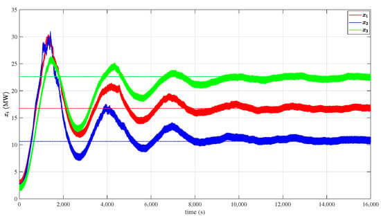
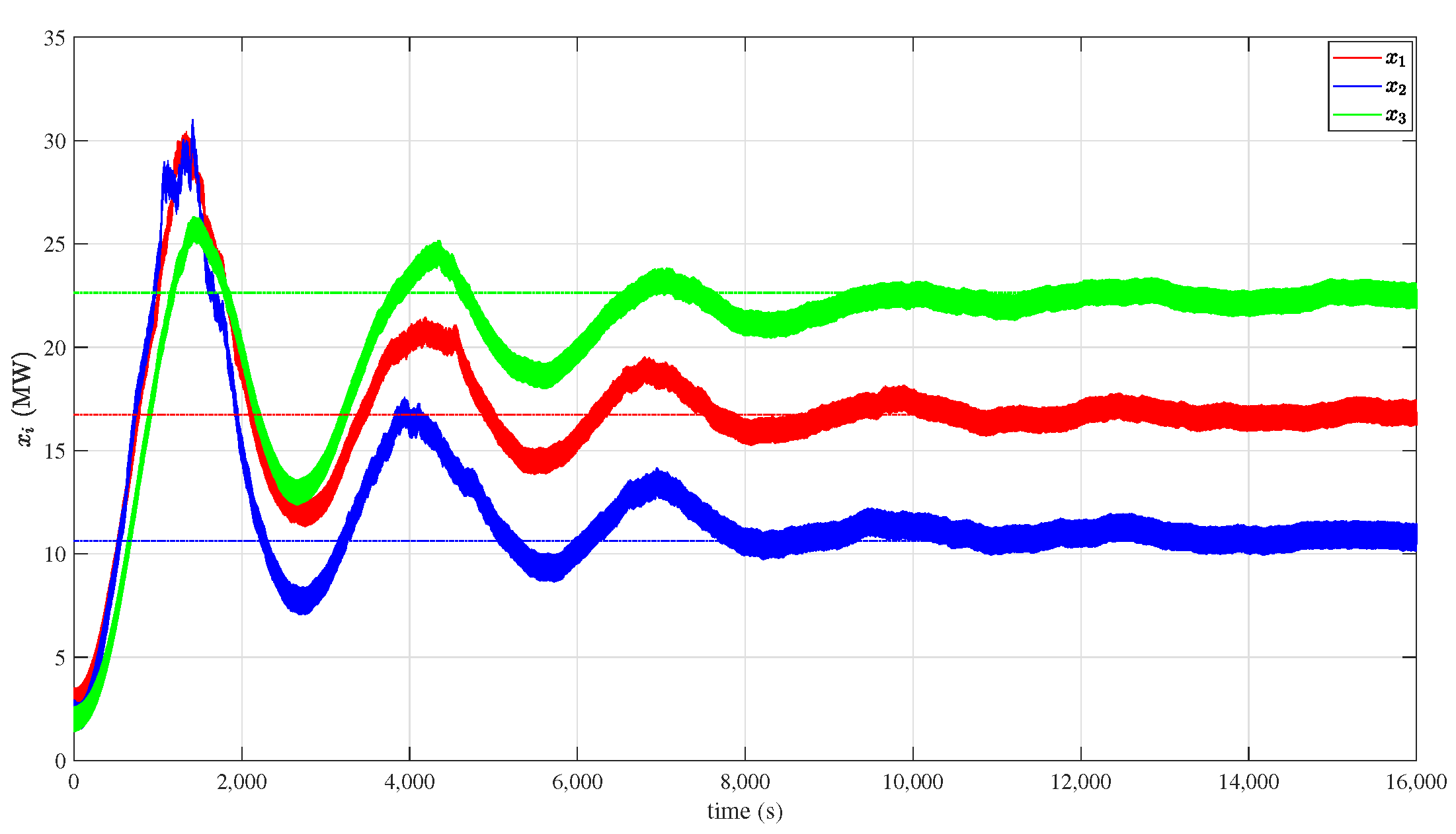
The first example is a three-generator microgrid under time delays. The cost function of generator i is $f_i\left(x_i\right)=h_i{x}_i^2+c_i{x}_i+s_i$, where the power output $x_i$ is measured in megawatts (MW) and $h_i>0$. In the quadratic form (10), $f_i\left(x_i\right)=\frac{1}{2}{x}_i^T{H}_i{x}_i+c_i^T{x}_i+s_i$, the gradient is $H_i{x}_i+c_i$, so this cost corresponds to the analysis matrix $H_i=2h_i$: the numerical coefficients enter the conditions of Theorem 1 through $H_i=2h_i$, not through $h_i$. The coefficient values are $h_1=0.088$, $h_2=0.0858$, $h_3=0.0902$, $c_1=1.22$, $c_2=2.34$, $c_3=0.0800$, and $s_1=s_2=s_3=0$, so that ${\lambda }_{\min }\left(H\right)=0.1716$ and ${\parallel H\parallel }_2=0.1804$. The total demand is 50 MW, with individual demands $d_1=20$ MW, $d_2=25$ MW, and $d_3=5$ MW. Solving (2) through the KKT conditions of Lemma 1 gives the optimal power outputs

$$x_1^{*}=16.7289\mathrm{MW},x_2^{*}=10.6310\mathrm{MW},x_3^{*}=22.6401\mathrm{MW},$$

(69)

at which the marginal costs $2h_i{x}_i^{*}+c_i$ are all equal to the multiplier $\overline{\lambda }=4.164$, as verified directly from the KKT conditions; ${\sum }_i{x}_i^{*}=50$ MW.

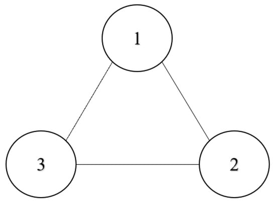
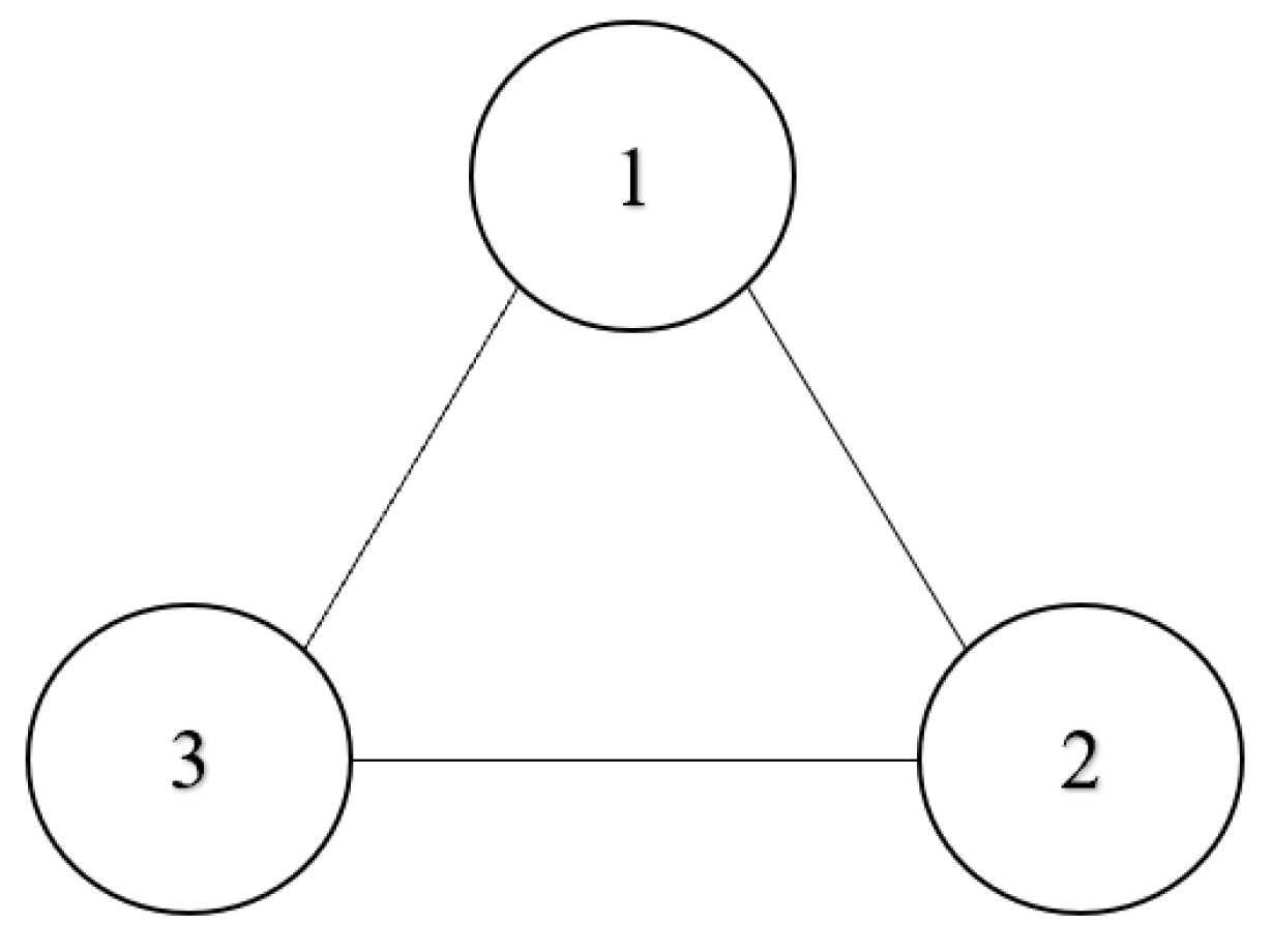
The connected undirected communication graph is shown in Figure 1; the weights are $a_{ij}=1$ on every edge. This graph is the complete graph $K_3$, for which ${\lambda }_2={\lambda }_N=3$ and ${\parallel \mathcal{L}\parallel }_2=3$.

Figure 1. Communication topology of the three-generator microgrid. The graph is the complete graph $K_3$ on the vertex set $\mathcal{V}=\{1,2,3\}$ with unit edge weights $a_{ij}=1$, so that $\mathcal{L}$ has eigenvalues ${\lambda }_1=0$ and ${\lambda }_2={\lambda }_3=3$, and ${\parallel \mathcal{L}\parallel }_2=3$. Edge $(i,j)$ carries the symmetric constant communication delays ${\tau }_{c_{12}}={\tau }_{c_{21}}=0.5$ s ${\tau }_{c_{13}}={\tau }_{c_{31}}=0.1$ s and ${\tau }_{c_{23}}={\tau }_{c_{32}}=0.4$ s, giving $N_0=3$ distinct delay values and ${\tau }_c^{*}=0.5$ s.

Measurement delays are $m_1=0.5$ s, $m_2=0.4$ s, $m_3=0.3$ s. Following Theorem 1, we set $\epsilon =0.006$, $q_1=39.5341$, $q_2=27.9152$, $q_3=49.8621$, $\alpha =0.0022$, $\beta =0.2$, $\gamma =0.0000011609$, $b_1=0.6$, $b_2=0.65$, $b_3=0.6$. The analysis parameters of Theorem 1 are $\kappa =72$, $\iota =3$ and $\rho =1.4\times {10}^3$. These are not controller gains, since the controller is fully specified by $(\alpha ,\beta ,\gamma ,b_i,q_{ij},\epsilon )$ together with the delays, but they are needed to evaluate the conditions (11)–(14) and the bound (68), and they are reported for that reason. Heterogeneous communication delays are $c_{12}=c_{21}=0.5$ s, $c_{13}=c_{31}=0.1$ s, $c_{23}=c_{32}=0.4$ s, so that $N_0=3$ distinct delays occur and ${\tau }_c^{*}=0.5$ s. The initial conditions are ${\widehat{x}}_1\left(0\right)=2.92$, ${\widehat{x}}_2\left(0\right)=2.289$, ${\widehat{x}}_3\left(0\right)=1.991$; ${\xi }_1\left(0\right)={\xi }_2\left(0\right)={\xi }_3\left(0\right)=0$, with the constant history $x_i\left(t\right)=0$ on $[-{\tau }^{*},0]$ (that is, ${\phi }_i$ in the notation of Section 3.1); ${\mu }_1\left(0\right)={\mu }_2\left(0\right)={\mu }_3\left(0\right)$, extended constantly on $[-{\tau }^{*},0]$; and $z_1\left(0\right)=z_2\left(0\right)=z_3\left(0\right)=0$.

With these values, the four conditions of Theorem 1 evaluate as follows. For $H=\mathrm{diag}(2h_1,2h_2,2h_3)$ we have ${\lambda }_{\min }\left(H\right)=0.1716$, ${\parallel H\parallel }_2=0.1804$ and ${\parallel H\parallel }_2^2=3.25\times {10}^{-2}$, so the required lower bound on $\kappa$ is ${(3+2\parallel H\parallel }_2^2)/{\lambda }_{\min }\left(H\right)-1=16.86$, which $\kappa =72$ satisfies. Condition (65) requires $\alpha <0.108$, satisfied by $\alpha =0.0022$. Condition (66) requires $\gamma <3.80\times {10}^{-6}$, satisfied by $\gamma =1.16\times {10}^{-6}$. The $\rho$-bounds (67) evaluate to ${\rho }_1=2.69\times {10}^4$ and ${\rho }_2=4.09\times {10}^3$, so that $\rho =1.4\times {10}^3$ satisfies (67). The resulting ${\varsigma }_1=0.493$, ${\varsigma }_2=5.21\times {10}^{-2}$ and ${\varsigma }_3=3.78\times {10}^3$ are all positive, and (14) gives $1-2\iota N{\beta }^2{\tau }_m^{*2}=0.82>0$. Condition (13) then requires ${\tau }_c^{*}<\sqrt{\rho /{\xi }_3}=0.61$ s, and condition (14) requires $\beta {\tau }_m^{*}<1/\sqrt{2\iota N}=0.236$, satisfied by $\beta {\tau }_m^{*}=0.1$. All simulated communication delays ($\le 0.5$ s) therefore lie within the theoretically admissible range.

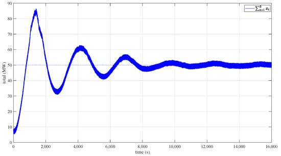
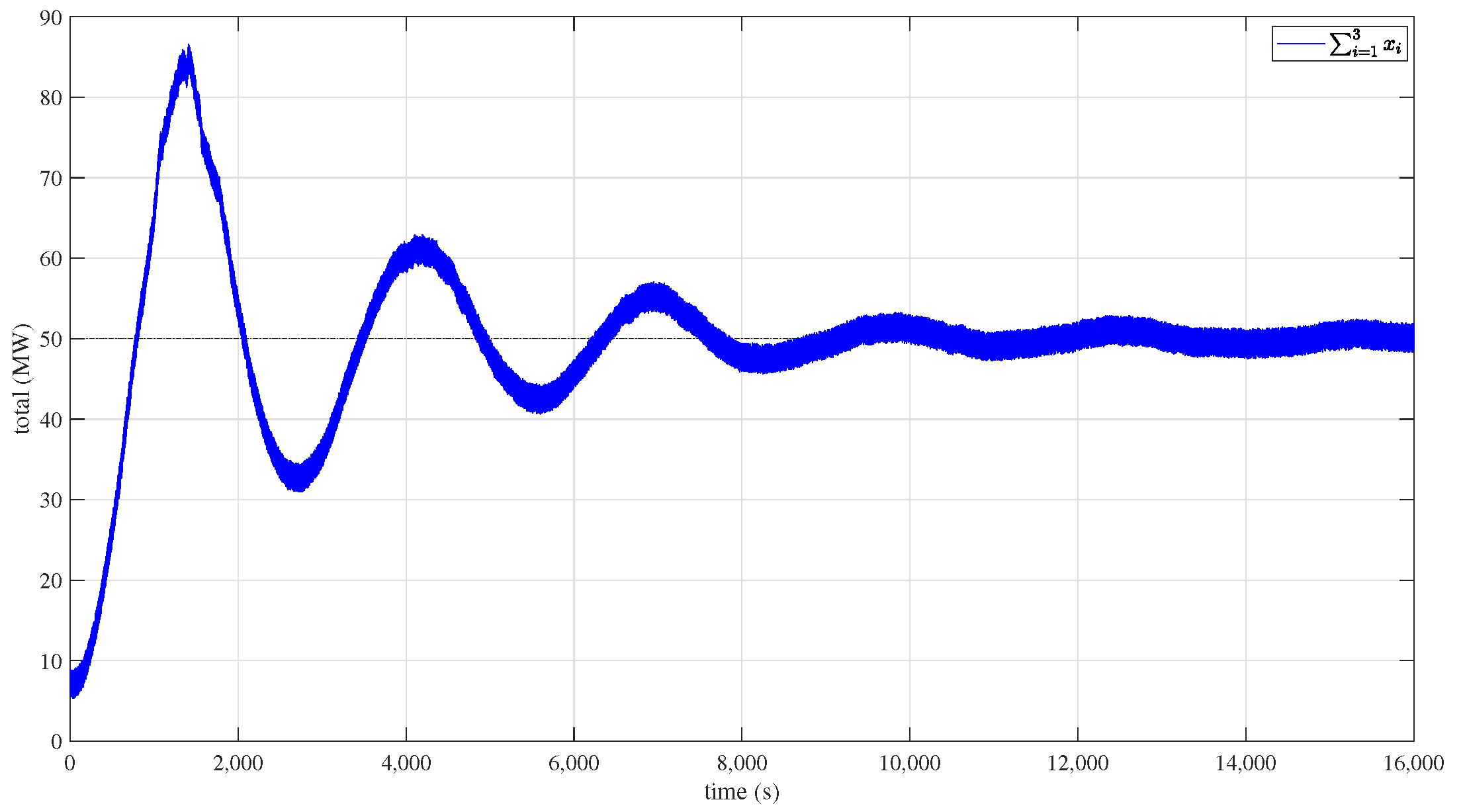
As shown in Figure 2 and Figure 3, the generator outputs converge to a small neighborhood of the optimal allocation (69), and the resource-constraint mismatch ${\sum }_i{x}_i\left(t\right)-{\sum }_i{d}_i$ converges to a small neighborhood of zero, in agreement with Theorem 1. In Figure 2, the dashed horizontal lines mark the optimal allocation (69) and the dash-dotted line marks the initial value; the estimates ${\widehat{x}}_i$ settle within a few percent of the optimal values after approximately $1.2\times {10}^4$ s, while the applied outputs $x_i$ exhibit the dither-induced residual of amplitude $b_i$ predicted by Remark 3. In Figure 3, the dashed line marks the total demand ${\sum }_i{d}_i=50$ MW; the total output, which starts from ${\sum }_i{\widehat{x}}_i\left(0\right)=7.2$ MW, settles in a neighborhood of 50 MW with a residual of the same order as the individual dithers.

Figure 2. Power outputs versus time, $t\in [0,1.6\times {10}^4]$ s. Abscissa: time t (s); ordinate: power (MW). Solid curves, drawn in black, are the applied generator outputs $x_1\left(t\right),x_2\left(t\right),x_3\left(t\right)$ of (4); dashed horizontal lines mark the optimal allocation $x_1^{*}=16.7289$ MW, $x_2^{*}=10.6310$ MW, $x_3^{*}=22.6401$ MW of (69); the dash-dotted line marks the initial estimate ${\widehat{x}}_1\left(0\right)=2.92$ MW. The estimates settle within a few percent of the dashed lines after approximately $1.2\times {10}^4$ s, with a dither-induced residual of amplitude $b_i$ ($0.6$, $0.65$, $0.6$ MW) consistent with Remark 3.

Figure 3. Total power output ${\sum }_i{x}_i\left(t\right)$ versus time, $t\in [0,1.6\times {10}^4]$ s. Abscissa: time t (s); ordinate: total power (MW). The dashed line marks the total demand ${\sum }_i{d}_i=50$ MW. The trajectory starts from ${\sum }_i{\widehat{x}}_i\left(0\right)=7.2$ MW and settles in a neighborhood of 50 MW, so that the supply–demand balance ${\sum }_i{x}_i\left(t\right)={\sum }_i{d}_i$ enforced by the integral channel of the PI consensus (Section 3.1) is satisfied up to the dither-induced residual.

4.2. Six-Generator Microgrid

The second example is a larger network of $N=6$ generators. The communication graph is the complete graph $K_6$ with unit edge weights, for which ${\lambda }_2={\lambda }_6=6$ and ${\parallel \mathcal{L}\parallel }_2=6$; it has 15 edges. Communication delays take the three values $0.1$, $0.2$ and $0.3$ s, assigned to five edges each, so that $N_0=3$ distinct delays occur and ${\tau }_c^{*}=0.3$ s. The measurement delays are ${\tau }_{m_1}=0.1$, ${\tau }_{m_2}=0.2$, ${\tau }_{m_3}=0.15$, ${\tau }_{m_4}=0.25$, ${\tau }_{m_5}=0.2$ and ${\tau }_{m_6}=0.3$ s, so that ${\tau }_m^{*}=0.3$ s.

The local costs are quadratic, $f_i\left(x_i\right)=h_i{x}_i^2+c_i{x}_i$, with $h_1=0.20$, $h_2=0.22$, $h_3=0.24$, $h_4=0.21$, $h_5=0.23$ and $h_6=0.25$, so that $H=\mathrm{diag}(0.40,0.44,0.48,0.42,0.46,0.50)$, and $c_1=2$, $c_2=4$, $c_3=1$, $c_4=5$, $c_5=3$, $c_6=2$, with $s_i=0$. The demands are $d_1=15$, $d_2=12$, $d_3=18$, $d_4=10$, $d_5=14$, $d_6=11$ MW, so the total demand is 80 MW. The KKT conditions of Lemma 1 give the optimal allocation

$$\begin{array}{cc}\hfill x_1^{*}& =17.1090\mathrm{MW},x_2^{*}=11.0082\mathrm{MW},x_3^{*}=16.3408\mathrm{MW},\hfill \\ \hfill x_4^{*}& =9.1514\mathrm{MW},x_5^{*}=12.7035\mathrm{MW},x_6^{*}=13.6872\mathrm{MW},\hfill \end{array}$$

(70)

at which the marginal costs $H_i{x}_i^{*}+c_i$ are all equal to $\overline{\lambda }=8.8436$.

The initial estimate is $\widehat{x}\left(0\right)=(3,2,4,2,3,2)$ MW, with ${\xi }_i\left(0\right)={\mu }_i\left(0\right)=z_i\left(0\right)=0$ and constant histories on $[-{\tau }^{*},0]$. The design parameters are $\alpha =0.004$, $\beta =0.2$, $\gamma =3.5\times {10}^{-5}$, $\epsilon =0.006$, $q=(30,35,28,40,32,36)$ and $b=(0.55,0.60,0.50,0.60,0.55,0.50)$ MW, while the analysis parameters are $\kappa =72$, $\iota =3$ and $\rho =1.4\times {10}^3$. The differential Equations (5)–(8) are integrated by the forward Euler scheme with step $2\times {10}^{-3}$ s, and the process (9) is sampled exactly from its transition law at the same step; the horizon is $2.4\times {10}^4$ s.

With $H=\mathrm{diag}(0.40,\dots ,0.50)$ we have ${\lambda }_{\min }\left(H\right)=0.40$ and ${\parallel H\parallel }_2=0.50$. The required lower bound on $\kappa$ is ${(3+2\parallel H\parallel }_2^2)/{\lambda }_{\min }\left(H\right)-1=7.75$, satisfied by $\kappa =72$. Condition (65) requires $\alpha <9.56\times {10}^{-2}$, satisfied by $\alpha =0.004$. Condition (66) requires $\gamma <3.76\times {10}^{-5}$, satisfied by $\gamma =3.5\times {10}^{-5}$. The bounds (67) evaluate to ${\rho }_1=3.92\times {10}^3$ and ${\rho }_2=2.25\times {10}^3$, so that $\rho =1.4\times {10}^3$ is admissible. The resulting ${\varsigma }_1=0.161$, ${\varsigma }_2=5.42\times {10}^{-2}$ and ${\varsigma }_3=7.11\times {10}^3$ are positive, and condition (13) requires ${\tau }_c^{*}<\sqrt{\rho /{\xi }_3}=0.444$ s, which holds for ${\tau }_c^{*}=0.3$ s. Condition (14) gives $1-2\iota N{\beta }^2{\tau }_m^{*2}=0.870>0$. All conditions of Theorem 1 are therefore satisfied; Table 2 collects the numerical values.

Table 2. Verification of the design conditions of Theorem 1 for the six-generator network of Section 4.2. The Requirement and Value entries are computed analytically from (11)–(14) and (65)–(68); they are not obtained by re-simulating the plant. The spectral quantities that enter the computation are ${\lambda }_{\min }\left(H\right)=0.40$, ${\parallel H\parallel }_2=0.50$, ${\lambda }_2=6$, ${\parallel \mathcal{L}\parallel }_2=6$ and $N_0=3$.

Quantity	Requirement	Value	Satisfied
$\kappa$	>$7.75$	72	Yes
$\alpha$	<$9.56\times {10}^{-2}$	$4.0\times {10}^{-3}$	Yes
$\gamma$	<$3.76\times {10}^{-5}$	$3.5\times {10}^{-5}$	Yes
$\rho$	<$2.25\times {10}^3$	$1.4\times {10}^3$	Yes
${\varsigma }_1,{\varsigma }_2$	>0	$0.161,5.42\times {10}^{-2}$	Yes
Equation (13), i.e., ${\tau }_c^{*}$	<$0.444$ s	$0.3$ s	Yes
Equation (14)	$1-2\iota N{\beta }^2{\tau }_m^{*2}>0$	$0.87$	Yes

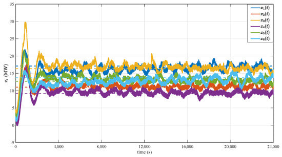
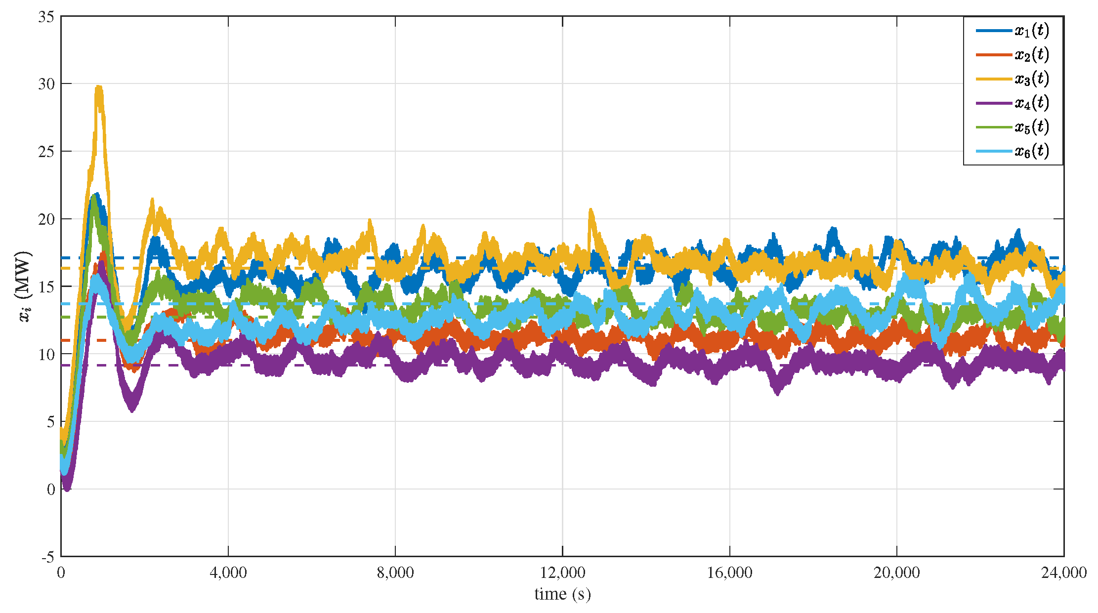
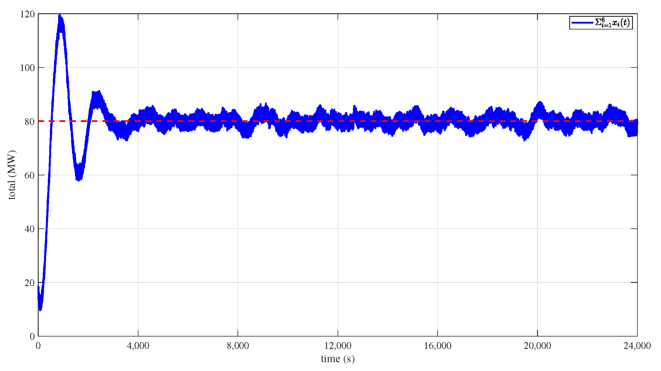
Figure 4 and Figure 5 show the resulting trajectories. After a transient of about 14,000 s, the generator outputs enter a neighborhood of the optimal allocation (70). Over the final 2400 s, the time-averaged applied outputs are $(16.68,11.31,16.27,9.34,12.91,13.65)$ MW, with a mean absolute deviation of $0.21$ MW ($0.26\%$ of the total demand) and a maximum deviation of $0.43$ MW. The total output settles around the demand 80 MW; its time-averaged absolute mismatch over the same window is $1.5$ MW, while the instantaneous excursions are of the order of a few megawatts, as expected from the six independent dithers and the residual fluctuations predicted by Remark 3. These results are consistent with Theorem 1 and show that the scheme remains effective when the network size is doubled and a heterogeneous delay profile with three distinct values is used.

Figure 4. Generator outputs versus time for the six-generator network, $t\in [0,$ 24,000] s. Abscissa: time t (s); ordinate: power (MW). Solid curves are the applied outputs $x_1\left(t\right),\dots ,x_6\left(t\right)$ of (4); dashed horizontal lines mark the optimal allocation (70). The estimates settle within a few tenths of a megawatt of the dashed lines after about $1.4\times {10}^4$ s, with the dither-induced residual of amplitude $b_i$ predicted by Remark 3.

Figure 5. Total power output ${\sum }_i{x}_i\left(t\right)$ versus time for the six-generator network, $t\in [0$, 24,000] s. Abscissa: time t (s); ordinate: total power (MW). The dashed line marks the total demand ${\sum }_i{d}_i=80$ MW. The total output settles in a neighborhood of the demand, with instantaneous fluctuations induced by the six dithers.

The numerical study covers two complete networks, the three-generator $K_3$ and the six-generator $K_6$, and therefore includes a larger network than the first example. The study remains illustrative rather than comprehensive: both networks are complete, the delay profiles are fixed, and no delay-free baseline or comparison with gradient-based schemes is reported. The title and formulation refer to allocation over networks on a general connected undirected graph, whereas the empirical evidence is restricted to two complete graphs; this gap is acknowledged. A systematic delay-sensitivity study, non-complete topologies, delay profiles approaching the bound (68), and a comparison against the gradient-based schemes of [24,25,26] are left for future work and are noted in the Conclusion. Table 2 and Table 3 report analytical verifications of the design conditions rather than re-runs of the plant simulation, because the analysis parameters $\kappa ,\iota ,\rho$ do not enter the controller and therefore leave the trajectories unchanged; the trajectories depend only on $(\alpha ,\beta ,\gamma ,b_i,q_{ij},\epsilon )$ and the delays.

Table 3. Verification of the design conditions of Theorem 1 for the parameters of Section 4. The Requirement and Value entries are computed analytically from the closed-form expressions (11)–(14) and (65)–(68); they are not obtained by re-simulating the plant. The spectral quantities that enter the computation are ${\lambda }_{\min }\left(H\right)=0.1716$, ${\parallel H\parallel }_2=0.1804$, ${\lambda }_2=3$ and ${\parallel \mathcal{L}\parallel }_2=3$, the last two because the communication graph is the complete graph $K_3$.

Quantity	Requirement	Value	Satisfied
$\kappa$	>$16.86$	72	Yes
$\alpha$	<$0.108$	$2.2\times {10}^{-3}$	Yes
$\gamma$	<$3.80\times {10}^{-6}$	$1.16\times {10}^{-6}$	Yes
$\rho$	<$\min \{2.69\times {10}^4,4.09\times {10}^3\}$	$1.4\times {10}^3$	Yes
${\varsigma }_1,{\varsigma }_2$	>0	$0.493,5.21\times {10}^{-2}$	Yes
Equation (13), i.e., ${\tau }_c^{*}$	<$0.61$ s	$0.5$ s	Yes
Equation (14)	$1-2\iota N{\beta }^2{\tau }_m^{*2}>0$	$0.82$	Yes

5. Conclusions

The optimal resource allocation problem over a connected undirected graph subject to measurement delays and heterogeneous constant communication delays was investigated. A distributed stochastic extremum seeking algorithm was proposed, which integrates the stochastic perturbation-based gradient estimation with a proportional–integral consensus protocol and relies solely on delayed local measurements of the individual objective functions. Under the quadratic-objective assumption of Section 3.2 (Assumption 4), stochastic averaging and Lyapunov stability theory were employed to demonstrate that the closed-loop trajectories converge almost surely, as the exploration timescale parameter vanishes, to an arbitrarily small neighborhood of the optimal allocation, in the practical sense. An explicit admissible range for the constant communication delays was derived, together with a sequential procedure for selecting the design parameters.

The following limitations delimit the scope of the present contribution.

Quadratic objectives. The convergence guarantee of Theorem 1 holds for the class of quadratic local objectives (Assumption 4). An extension to general strongly convex objectives via a Taylor-remainder argument is not available, as Remark 2 shows; it would require a rigorous two-time-scale perturbation analysis and remains open. Constant, symmetric delays. The delay bound (68) is derived for constant communication delays with ${\tau }_{c_{ij}}={\tau }_{c_{ji}}$ on an undirected, fixed graph (Assumption 3); see Remark 1. Averaging theorem. The final averaging step uses Theorem 4.7 of [32]. The framework, its four hypotheses and the three conclusions drawn from them are stated in Appendix B.1, verified one by one for the present multiple-delay system in Appendix B.3, and assembled into the chain that yields (15) in Appendix B.4, but the theorem itself is not reproved here (Appendix B.1). The quadratic restriction is inherited at this step, and its location is identified in Appendix B.5. Numerical scope. The numerical study reports two scenarios, a three-generator microgrid and a six-generator microgrid, together with analytical verifications of the design conditions (Table 2 and Table 3), rather than a systematic delay-sensitivity study. Both networks are complete graphs, so the empirical support for the theory remains illustrative rather than comprehensive; a delay-free baseline, non-complete topologies, and delay profiles near the bound (68) are the natural next experiments and are listed below.

The proposed framework is restricted to connected, undirected, fixed graphs with constant, symmetric delays known a priori. Extensions to directed and time-varying topologies, to time-varying and asymmetric delays, to asynchronous communication and non-complete or switching networks, to systematic numerical comparisons with gradient-based delay-aware schemes, and to an input-to-state stability (ISS) analysis under persistent disturbances are left as open directions.

Appendix A.1. Origin of the Functional (51)

The error system (43)–(48) has three structurally different blocks. The first block, (43)–(45), is the “matched” pair $({\tilde{\mathbf{x}}}_1^{♯},{\tilde{\mu }}_1^{♯})$ along the consensus direction, whose dynamics are free of the Laplacian and of the communication delay; this is why $V_1$ contains the terms $\frac{1}{2}\kappa {|{\tilde{\mathbf{x}}}_1^{♯}-{\tilde{\mu }}_1^{♯}|}^2$, $\frac{1}{2}{\kappa }^2{\left|{\tilde{\mathbf{x}}}_1^{♯}\right|}^2$ and $\frac{1}{2}{\kappa }^2{\left|{\tilde{\mu }}_1^{♯}\right|}^2$, with the large weight $\kappa$ on the mismatch term. The second block, (46)–(48), is the disagreement pair $({\tilde{\mu }}_2^{♯},{\tilde{\mathbf{z}}}_2^{♯})$ coupled through the delay-weighted operators $R^T{\mathcal{L}}^{\left(p\right)}R$; the corresponding terms in $V_1$ are grouped as $\frac{1}{2}\kappa {|{\tilde{\mu }}_2^{♯}+{\tilde{\mathbf{z}}}_2^{♯}|}^2$, $\frac{1}{2}\alpha \kappa (\kappa +1){\left|{\tilde{\mathbf{z}}}_2^{♯}\right|}^2$ and $\frac{1}{2}\kappa (\kappa -1){\left|{\tilde{\mu }}_2^{♯}\right|}^2$, whose weights are chosen so that the Laplacian-weighted quadratic form produced by differentiating (46)–(48) is negative definite. The third block, (49) and (50), is the measurement-delay error $\zeta$, which is handled separately by $V_2$ in (59) because its dynamics $\dot{\zeta }=-\beta \zeta (t-{\tau }_m)$ involve a different delay channel. Finally, the term $\frac{1}{2\gamma }\alpha (1-\alpha )\kappa (\kappa +1){\tilde{\mathbf{z}}}_2^{♯T}({\mathrm{\Lambda }}^{-1}\otimes I_n){\tilde{\mathbf{z}}}_2^{♯}$ uses the existence of ${\mathrm{\Lambda }}^{-1}$ (the positive Laplacian eigenvalues are bounded away from zero) to convert the ${\tilde{\mathbf{z}}}_2^{♯T}{\tilde{\mu }}_2^{♯}$ cross term arising from (46)–(48) into a negative contribution; this is where the smallest positive eigenvalue ${\lambda }_2$ enters the analysis, through $\parallel {\mathrm{\Lambda }}^{-1}{\parallel }_2\le 1/{\lambda }_2$.

Appendix A.2. Differentiation and the Delay-Induced Terms

Differentiating $V_1$ along (43)–(48) and replacing ${\tilde{\mu }}_2^{♯}(t-{\tau }_p)$ by ${\tilde{\mu }}_2^{♯}\left(t\right)-{\int }_{t-{\tau }_p}^t{\dot{\tilde{\mu }}}_2^{♯}\left(s\right)\mathrm{d}s$ produces (52), in which the delay enters only through the terms ${\Delta }_{{\tilde{\mu }}_2^{♯}}^{\left(p\right)}$. This is the standard Krasovskii step: the delayed state is written as the current state minus an integral of the derivative, so that the delay dependence is isolated in integral terms that can be bounded.

Appendix A.3. Term-by-Term Young’s Inequality: The Passage from (52) to (53)

Write $Q={\mathrm{\Lambda }}^{-1}\otimes I_n\succ 0$, so that ${\parallel Q\parallel }_2=1/{\lambda }_2$, and recall $\parallel R^T\otimes I_n{\parallel }_2\le 1$, whence $\parallel {\tilde{\mathbf{x}}}_2^{♯}\parallel \le \parallel {\tilde{\mathbf{x}}}^a\parallel$ and ${\tilde{\mathbf{x}}}_2^{♯T}Q{\tilde{\mathbf{x}}}_2^{♯}\le {\lambda }_2^{-1}{\parallel {\tilde{\mathbf{x}}}^a\parallel }^2$. Each mixed product in (52) is bounded with Young’s inequality in the form $a^{T}b\le {\rho \parallel a\parallel }^2+{\parallel b\parallel }^2/\left(4\rho \right)$, $\rho >0$, applied to the splitting indicated; the free parameter $\rho$ is fixed by the coefficient that the bound is required to produce. One obtains the seven termwise estimates

$$\begin{array}{cc}\hfill -\alpha \kappa {\tilde{\mathbf{x}}}^{aT}H{\tilde{\mu }}^a& \le {\alpha \kappa \parallel H\parallel }_2^2{\tilde{\mathbf{x}}}^{aT}{\tilde{\mathbf{x}}}^a+{\displaystyle \frac{\alpha \kappa }{4}}{\tilde{\mu }}^{aT}{\tilde{\mu }}^a,\hfill \end{array}$$

(A1)

$$\begin{array}{cc}\hfill -{\alpha }^2\kappa (\kappa +1){\tilde{\mathbf{z}}}_2^{♯T}\left(R^T\otimes I_n\right)H{\tilde{\mathbf{x}}}^a& \le {\displaystyle \frac{\alpha \kappa (\kappa +1)}{2}}{\tilde{\mathbf{x}}}^{aT}H{\tilde{\mathbf{x}}}^a+{\displaystyle \frac{{\alpha }^3\kappa (\kappa +1){\parallel H\parallel }_2}{2}}{\tilde{\mathbf{z}}}_2^{♯T}{\tilde{\mathbf{z}}}_2^{♯},\hfill \end{array}$$

(A2)

$$\begin{array}{cc}\hfill \alpha \kappa (\kappa +1){\tilde{\mathbf{x}}}^{aT}\zeta & \le {\displaystyle \frac{\alpha \kappa }{2}}{\tilde{\mathbf{x}}}^{aT}{\tilde{\mathbf{x}}}^a+{\displaystyle \frac{\alpha \kappa {(\kappa +1)}^2}{2}}{\zeta }^T\zeta ,\hfill \end{array}$$

(A3)

$$\begin{array}{cc}\hfill -\alpha \kappa {\tilde{\mu }}^{aT}\zeta & \le {\displaystyle \frac{\alpha \kappa }{4}}{\tilde{\mu }}^{aT}{\tilde{\mu }}^a+\alpha \kappa {\zeta }^T\zeta ,\hfill \end{array}$$

(A4)

$$\begin{array}{cc}\hfill {\alpha }^2\kappa (\kappa +1){\tilde{\mathbf{z}}}_2^{♯T}{\zeta }_2^{♯}& \le {\displaystyle \frac{{\alpha }^3\kappa (\kappa +1)}{2}}{\tilde{\mathbf{z}}}_2^{♯T}{\tilde{\mathbf{z}}}_2^{♯}+{\displaystyle \frac{\alpha \kappa (\kappa +1)}{2}}{\zeta }_2^{♯T}{\zeta }_2^{♯},\hfill \end{array}$$

(A5)

$$\begin{array}{cc}\hfill \gamma \kappa (\kappa +2){\tilde{\mathbf{x}}}_2^{♯T}Q{\tilde{\mu }}_2^{♯}& \le \gamma {(\kappa +2)}^2{\tilde{\mathbf{x}}}_2^{♯T}Q{\tilde{\mathbf{x}}}_2^{♯}+{\displaystyle \frac{\gamma {\kappa }^2}{4}}{\tilde{\mu }}_2^{♯T}Q{\tilde{\mu }}_2^{♯},\hfill \end{array}$$

(A6)

$$\begin{array}{cc}\hfill {\alpha }^2{(\kappa +1)}^2\gamma {\tilde{\mathbf{z}}}_2^{♯T}Q{\tilde{\mu }}_2^{♯}& \le {\displaystyle \frac{{\alpha }^4{(\kappa +1)}^4}{{\kappa }^2}}\gamma {\tilde{\mathbf{z}}}_2^{♯T}{\tilde{\mathbf{z}}}_2^{♯}+{\displaystyle \frac{\gamma {\kappa }^2}{4}}{\tilde{\mu }}_2^{♯T}Q{\tilde{\mu }}_2^{♯}.\hfill \end{array}$$

(A7)

Adding (A1)–(A7) to the base terms of (52) and using ${\tilde{\mathbf{x}}}^{aT}H{\tilde{\mathbf{x}}}^a\ge {\lambda }_{\min }\left(H\right){\parallel {\tilde{\mathbf{x}}}^a\parallel }^2$, ${\zeta }_2^{♯T}{\zeta }_2^{♯}\le {\zeta }^T\zeta$ and ${\tilde{\mathbf{x}}}_2^{♯T}Q{\tilde{\mathbf{x}}}_2^{♯}\le {\lambda }_2^{-1}{\parallel {\tilde{\mathbf{x}}}^a\parallel }^2$ produces (53). Concretely, the half-weighted terms combine as follows: the two quantities $\frac{1}{2}\kappa (\kappa +1){\tilde{\mathbf{x}}}^{aT}H{\tilde{\mathbf{x}}}^a$ from (A2) and $\alpha \kappa (\kappa +1){\tilde{\mathbf{x}}}^{aT}H{\tilde{\mathbf{x}}}^a$ from the base term of (52) give the negative H-term $-\frac{1}{2}\kappa \alpha (\kappa +1){\tilde{\mathbf{x}}}^{aT}H{\tilde{\mathbf{x}}}^a$; the three positive ${\tilde{\mathbf{x}}}^{aT}{\tilde{\mathbf{x}}}^a$ contributions ${\alpha \kappa \parallel H\parallel }_2^2$ from (A1), $\frac{1}{2}\alpha \kappa$ from (A3) and $\alpha \kappa$ from the base term collect into $\frac{1}{2}{\kappa \alpha (3+2\parallel H\parallel }_2^2)$; and the term $\gamma {(\kappa +2)}^2{\tilde{\mathbf{x}}}_2^{♯T}Q{\tilde{\mathbf{x}}}_2^{♯}$ from (A6) contributes, through the relation ${\tilde{\mathbf{x}}}_2^{♯T}Q{\tilde{\mathbf{x}}}_2^{♯}\le {\lambda }_2^{-1}{\parallel {\tilde{\mathbf{x}}}^a\parallel }^2$, the Laplacian term $-\frac{1}{2}\kappa \left(-2/\left(\kappa {\lambda }_2\right)\gamma {(\kappa +2)}^2\right)$ recorded in the brace of (53). In the same way the two $\frac{\alpha \kappa }{4}$ contributions to ${\tilde{\mu }}^{aT}{\tilde{\mu }}^a$ combine with the base term $-\alpha \kappa$ to give $-\frac{1}{2}\alpha \kappa$, and the ${\tilde{\mathbf{z}}}_2^{♯}$ coefficients of (A2), (A5) and (A7) reorganize into the bracket of (53).

Appendix A.4. The Integral Terms: The Passage from (53) to (55)

Let $S={\sum }_{p=1}^{N_0}{\Delta }_{{\tilde{\mu }}_2^{♯}}^{\left(p\right)}$ and $J={\int }_{t-{\tau }_c^{*}}^t{\tilde{\mu }}_2^{♯T}\left(s\right){\tilde{\mu }}_2^{♯}\left(s\right)\mathrm{d}s$. Inequality (54)—obtained from the Cauchy–Schwarz inequality applied to S, together with $\parallel {\mathcal{L}}^{\left(p\right)}{\parallel }_2\le {\parallel \mathcal{L}\parallel }_2$ and Jensen’s inequality applied to the resulting $N_0$-fold sum of integrals over intervals of length ${\tau }_p\le {\tau }_c^{*}$—reads $S^{T}S\le N_0^2{\parallel \mathcal{L}\parallel }_2^2{\tau }_c^{*}J$. Applying the same Young inequality to the four S-dependent products in (53) yields

$$\begin{array}{cc}\hfill -\gamma \kappa {\tilde{\mu }}_2^{♯T}S& \le {\displaystyle \frac{\gamma \kappa }{4}}{\tilde{\mu }}_2^{♯T}{\tilde{\mu }}_2^{♯}+\gamma \kappa N_0^2{\parallel \mathcal{L}\parallel }_2^2{\tau }_c^{*}J,\hfill \end{array}$$

(A8)

$$\begin{array}{cc}\hfill \gamma \kappa (\kappa +2){\tilde{\mathbf{x}}}_2^{♯T}S& \le {\displaystyle \frac{\gamma {(\kappa +2)}^2}{2{\lambda }_2}}{\tilde{\mathbf{x}}}_2^{♯T}{\tilde{\mathbf{x}}}_2^{♯}+{\displaystyle \frac{\gamma {\kappa }^2{\lambda }_2}{2}}{N}_0^2{\parallel \mathcal{L}\parallel }_2^2{\tau }_c^{*}J,\hfill \end{array}$$

(A9)

$$\begin{array}{cc}\hfill {\alpha }^2{(\kappa +1)}^2\gamma {\tilde{\mathbf{z}}}_2^{♯T}S& \le {\displaystyle \frac{{\alpha }^4{(\kappa +1)}^4}{4{\kappa }^2}}\gamma {\tilde{\mathbf{z}}}_2^{♯T}{\tilde{\mathbf{z}}}_2^{♯}+\gamma {\kappa }^2{N}_0^2{\parallel \mathcal{L}\parallel }_2^2{\tau }_c^{*}J,\hfill \end{array}$$

(A10)

$$\begin{array}{cc}\hfill \alpha (1-\alpha )\kappa (\kappa +1){\tilde{\mathbf{z}}}_2^{♯T}QS& \le {\displaystyle \frac{\alpha \kappa }{2}}{\tilde{\mathbf{z}}}_2^{♯T}{\tilde{\mathbf{z}}}_2^{♯}+{\displaystyle \frac{\alpha {(1-\alpha )}^2\kappa {(\kappa +1)}^2}{2{\lambda }_2^2}}{N}_0^2{\parallel \mathcal{L}\parallel }_2^2{\tau }_c^{*}J.\hfill \end{array}$$

(A11)

Substituting (A8)–(A11) into (53) and collecting coefficients yields (55). The $\tilde{\mu }$-type contributions combine as follows: the term $\frac{\gamma \kappa }{4}{\tilde{\mu }}_2^{♯T}{\tilde{\mu }}_2^{♯}$ of (A8), bounded by $\frac{\gamma \kappa }{4}{\tilde{\mu }}^{aT}{\tilde{\mu }}^a$, adds to the base coefficient $-\frac{1}{2}\alpha \kappa$ to give $-(\frac{1}{2}\alpha -\frac{1}{4}\gamma )\kappa$ for ${\tilde{\mu }}^{aT}{\tilde{\mu }}^a$; the two quantities $\frac{\gamma {\kappa }^2}{4}{\tilde{\mu }}_2^{♯T}Q{\tilde{\mu }}_2^{♯}$ from (A6) to (A7) add to the base term $-\gamma {\kappa }^2$ to give $-\frac{1}{2}\gamma {\kappa }^2$; and the two quantities $\frac{\alpha \kappa }{2}{\tilde{\mathbf{z}}}_2^{♯T}{\tilde{\mathbf{z}}}_2^{♯}$ and $\frac{{\alpha }^4{(\kappa +1)}^4}{4{\kappa }^2}\gamma {\tilde{\mathbf{z}}}_2^{♯T}{\tilde{\mathbf{z}}}_2^{♯}$ from (A10) to (A11) add to the ${\tilde{\mathbf{z}}}_2^{♯}$ bracket carried from (53), producing the coefficient displayed in (55). The integral coefficient is

$$\begin{array}{c}\hfill \gamma \kappa \left(1+\kappa +{\displaystyle \frac{\kappa {\lambda }_2}{2}}\right)+{\displaystyle \frac{\alpha {(1-\alpha )}^2\kappa {(\kappa +1)}^2}{2{\lambda }_2^2}},\end{array}$$

which, multiplied by $N_0^2{\parallel \mathcal{L}\parallel }_2^2$, is exactly ${\varsigma }_3$ in Theorem 1; the factor ${\lambda }_2^2$ in the second term reflects the two factors $\parallel {\mathrm{\Lambda }}^{-1}{\parallel }_2=1/{\lambda }_2$ entering (A11).

Appendix A.5. Handling the Residual Integral and the ζ Term

The residual nonnegative integral in (55) is compensated by $V_1^{\tilde{\mu }}$ with weight $\rho /{\tau }_c^{*}$ as in (57), which is what produces conditions (11)–(13); explicitly, the terms $4\rho ({\alpha }^2+{\gamma }^2\parallel \mathcal{L}{\parallel }_2^2)$ and $4\rho {\alpha }^2$ obtained from (56) are subtracted from the coefficients of ${\tilde{\mathbf{x}}}^{aT}{\tilde{\mathbf{x}}}^a$ and ${\tilde{\mathbf{z}}}_2^{♯T}{\tilde{\mathbf{z}}}_2^{♯}$, giving ${\varsigma }_1$ and ${\varsigma }_2$. The residual nonnegative term ${\xi }_4{\zeta }^T\zeta$ is handled by $V_2$ in (59): the factor $\iota$ and the condition (14) ensure that ${\dot{V}}_2$ in (60) has a sufficiently negative leading coefficient to dominate the delayed term, and $V_2^{♯}$ is the Krasovskii functional that absorbs ${\int }_{t-2{\tau }_m^{*}}^t{V}_2\left(s\right)\mathrm{d}s$, mirroring the role of $V_1^{\tilde{\mu }}$ for the communication-delay channel. Conditions (11)–(14) thus arise from the two distinct delay channels, and this separation is why the measurement and communication delays can be tuned independently through $\rho$ and $\beta$ respectively.

Appendix B.1. The Averaging Framework of [32]

The final step of the proof of Theorem 1 uses the stochastic averaging theorem of our companion paper ([32], Theorem 4.7), which generalizes the single-delay result of [35] to multiple delays and reduces to the delay-free result of [29] when all delays vanish; the single-delay result rests in turn on the classical small-parameter averaging theory of Khasminskii [36]. The relation to [36] is as follows. Khasminskii averages the single-scale perturbation of $\dot{x}=\epsilon F(x,t,\omega )$ under a Lipschitz condition in the state that is required to hold for all t and almost every $\omega$, hence globally, and under a law-of-large-numbers hypothesis; his averaged equation is ordinary, and his conclusion is convergence in the mean, uniformly on a compact time interval. The framework stated here differs in three connected respects: its averaged field (A14) is evaluated along the delayed arguments $X(t-h_0),\dots ,X(t-h_l)$ and the comparison in Lemma A1 is made on the delay system (A12) and (A13) rather than on an ODE; the Lipschitz condition of Assumption A1 is local, holding on balls of radius c, not global; and the convergence is almost sure, obtained from stationarity and ergodicity through Birkhoff’s theorem rather than in the mean. The first two differences bear on existence: in the classical setting, the global Lipschitz condition makes the existence and uniqueness of the solution of the original equation on the whole half-line immediate, whereas with a local condition and delayed arguments this is not immediate for (A12) and (A13) and is established in Appendix B.3.4. The framework’s single-delay specialization is the result of [35], and its delay-free specialization is the Khasminskii-type averaging of [36], as developed for extremum seeking in [29]. Because that theorem is central to the argument, this appendix states it together with its assumptions and verifies them here, so that the reliance on [32] is explicit rather than implicit and no claim of proof independent of [32] is made: Specifically, Appendix B.1 states the framework, Appendix B.2 records which hypothesis each conclusion rests on, Appendix B.3 verifies every hypothesis for system (4)–(8), Appendix B.4 assembles the chain that produces (15), and Appendix B.5 isolates the step at which the quadratic restriction of Assumption 4 enters the argument.

Numbering. The equations reproduced from [32] are numbered (A12)–(A17) so that they cannot be confused with the equations of this paper.

Consider the nonlinear delay system with stochastic perturbation

$$\begin{array}{cc}\hfill {\displaystyle \frac{\mathrm{d}X\left(t\right)}{\mathrm{d}t}}& =f\left(X(t-h_0),X(t-h_1),\dots ,X(t-h_l),Y(t/\epsilon )\right),t>0,\hfill \end{array}$$

(A12)

$$\begin{array}{cc}\hfill X\left(t\right)& =X_0\left(t\right),\forall t\in [-h,0],\hfill \end{array}$$

(A13)

where $0=h_0<h_1\le \cdots \le h_l=h$ are constant time delays ($h_0=0$ accounts for the undelayed terms), l is a positive integer, $\left\{Y\right(t),t\ge 0\}$ is a time-homogeneous continuous-time Markov process defined on a complete probability space, taking values in $S_Y\subset {\mathbb{R}}^m$, $X_0\in {𝒞}_n^h$ is a deterministic continuous history, and $\epsilon \in (0,{\epsilon }_0)$ with ${\epsilon }_0>0$ fixed.

The framework rests on four assumptions.

Assumption A1 

([32], Assumption 4.1). $f(x_0,\dots ,x_l,y)$ is a continuous function of $(x_0,\dots ,x_l,y)$; for every fixed $(x_0,\dots ,x_l)$ the map $y\mapsto f(x_0,\dots ,x_l,y)$ is bounded; and for every $c>0$, there exists $L_c>0$ such that, for all $x_i,{\tilde{x}}_i\in {\mathbb{R}}^n$ and all $y\in S_Y$ with $\max \{\parallel x_0\parallel ,\parallel {\tilde{x}}_0\parallel ,\dots ,\parallel x_l\parallel ,\parallel {\tilde{x}}_l\parallel \}$$\le c$,

$$\begin{array}{c}\hfill \parallel f(x_0,\dots ,x_l,y)-f({\tilde{x}}_0,\dots ,{\tilde{x}}_l,y)\parallel \le L_c{\displaystyle \sum _{i=0}^l}\parallel x_i-{\tilde{x}}_i\parallel .\end{array}$$

Assumption A2 

([32], Assumption 4.2). For every history, $X_0\in {𝒞}_n^h$ and every perturbation path $\left\{Y\right(t),t\ge 0\}$, System (A12) and (A13) has a unique solution on $[-h,+\infty )$ almost surely.

Assumption A3 

([32], Assumption 4.3). $\left\{Y\right(t),t\ge 0\}$ is a stationary ergodic process with invariant distribution μ.

Assumption A4 

([32], [Assumption 4.4). System (A14) and (A15) has a solution on $[-h,+\infty )$.

Under these assumptions, the following three results hold; they are the results used in the present paper.

The averaged system associated with (A12) and (A13) is defined by

$$\begin{array}{cc}\hfill {\displaystyle \frac{\mathrm{d}\overline{X}\left(t\right)}{\mathrm{d}t}}& =\overline{f}\left(\overline{X}(t-h_0),\overline{X}(t-h_1),\dots ,\overline{X}(t-h_l)\right),t>0,\hfill \end{array}$$

(A14)

$$\begin{array}{cc}\hfill \overline{X}\left(t\right)& =X_0\left(t\right),\forall t\in [-h,0],\hfill \end{array}$$

(A15)

with the averaged vector field

$$\begin{array}{c}\hfill \overline{f}(x_0,\dots ,x_l)={\int }_{S_Y}f(x_0,\dots ,x_l,y)\mu \left(\mathrm{d}y\right).\end{array}$$

Lemma A1 

([32], Lemma 4.5). Let Assumptions A1–A4 hold. Then, for every $T>0$,

$$\begin{array}{c}\hfill \underset{\epsilon \to 0}{\lim }\underset{t\in [-h,T]}{\sup }\parallel X\left(t\right)-\overline{X}\left(t\right)\parallel =0,a.s.\end{array}$$

(A16)

Theorem A1 

([32], Theorem 4.6). Let Assumptions A1–A4 hold. Then, for every $\delta >0$,

$$\begin{array}{c}\hfill \underset{\epsilon \to 0}{\lim }\inf \left\{t\ge -h:\parallel X\left(t\right)-\overline{X}\left(t\right)\parallel >\delta \right\}=+\infty ,a.s.\end{array}$$

Theorem A2 

([32], Theorem 4.7). Let Assumptions A1–A4 hold. If the origin is a locally exponentially stable equilibrium point of the averaged system (A14) and (A15), then the solution of (A12) and (A13) is weakly exponentially convergent, that is, there exist $r>0$, $\mu >0$ and $\nu >0$ such that for every initial history $X_0\in \{\phi \in {𝒞}_n^h:\parallel \phi \parallel <r\}$ and every $\delta >0$,

$$\begin{array}{c}\hfill \underset{\epsilon \to 0}{\lim }\inf \left\{t\ge -h:\parallel X\left(t\right)\parallel >\mu \parallel X_0\parallel \exp \{-\nu t\}+\delta \right\}=+\infty ,a.s.\end{array}$$

(A17)

As ([32], Remark 3) explains, the adverb “weakly” in Theorem A2 records two features of (A17): the statement is asymptotic in $\epsilon$, and it is expressed through the first exit time from a set, so that it asserts convergence to a $\delta$-neighborhood of the origin rather than to the origin itself. This is the reading adopted in (15) and Remark 3, and it is why this paper does not read (15) as exponential convergence to the optimum: the qualifier is [32]’s, and (A17) is a practical convergence statement.

The logical division between the two results deserves comment, because it determines the quantifier of (15). Theorem A1 is an approximation statement and carries no stability assertion of its own: it says that the solution of the original system follows that of the averaged system, uniformly on every compact interval (A16) and, in first-exit form, over arbitrarily long ones. Theorem A2 adds the stability of the averaged system. Its hypothesis is the local exponential stability of the averaged origin, its conclusion is (A17), and the restriction to $\parallel X_0\parallel <r$ is inherited from the neighborhood on which the averaged Lyapunov function is defined, not from the approximation step, which is available for every initial history.

Two qualifications bear on the quantifier of (15). First, the conclusion is the weak one of (A17): it places the trajectory in a $\delta$-neighborhood of the origin at the averaged rate, and it asserts no rate for $\parallel X\left(t\right)\parallel$ itself, since the $\delta$-term cannot be removed at fixed $\epsilon$.

Second, the transfer can be made global in the initial history, and for the present problem it is. The averaged error system (37)–(40) is linear, so its exponential stability is global: the estimate (64) holds with the same rate for every initial history, and the constants relating V to the norm are uniform. There are therefore $\overline{\mu },\nu >0$ with $\parallel \overline{X}\left(t\right)\parallel \le \overline{\mu }\parallel X_0\parallel e^{-\nu t}$ for all $t\ge -{\tau }^{*}$ and every $X_0$. Fix $X_0$ and $T>0$. By Appendix B.3.4, for every sufficiently small $\epsilon$, the stopped comparison holds with $M={\sup }_{t\in [-{\tau }^{*},T]}\left|\overline{X}\left(t\right)\right|+1$, and M is bounded uniformly in T because $\overline{X}$ decays. Since ${\psi }_T\left(\epsilon \right)\to 0$ almost surely, for every $\delta >0$ and every sufficiently small $\epsilon$, the solution satisfies $\parallel X\left(t\right)\parallel \le \overline{\mu }\parallel X_0\parallel e^{-\nu t}+\delta$ on $[-{\tau }^{*},T]$. As $T>0$ is arbitrary and (15) is a limit statement in $\epsilon$, this yields (15) for every finite $X_0$; since $\parallel X_0\parallel$ and $\psi \left(0\right)$ are equivalent with constants independent of the initial history (A15), the envelope can be written as in (15). The convergence is pointwise in the initial history and not uniform over it, because the threshold on $\epsilon$ depends on $X_0$ and on the realization.

Appendix B.2. Which Assumption Yields Which Conclusion

The logical role of each assumption is as follows, and the verification in Appendix B.3 follows this order.

Assumption A1 is what makes the argument work at all: it gives the local Lipschitz property of f needed for the comparison estimates, and, since $\overline{f}$ averages f over y and is therefore locally Lipschitz itself, it makes the averaged field $\overline{f}$ locally Lipschitz as required in the proof of Lemma A1. Its boundedness-in-y clause is what allows the increment $f(·,y)-\overline{f}(·)$ to be bounded by an $O\left(\epsilon \right)$-type quantity along the fast motion. Assumption A2 makes the solution of the original system well-defined on the whole half-line, so that the stopping-time argument used in the proof of Lemma A1 can be terminated. Assumption A3 is what gives the invariant measure $\mu$ and licenses the ergodic average that replaces the fast oscillation by its mean; it is the hypothesis under which $\overline{f}$ is the correct limit field. Assumption A4 makes the averaged solution $\overline{X}$ well defined on the whole half-line, which is needed both for the comparison in Lemma A1 and for the stability statement in Theorem A2.

Appendix B.3. Verification of Assumptions A1–A4 for System (4)–(8)

Appendix B.3.1. Reduction of (4)–(8) to the Form (A12) and (A13)

Take as slow state

$$\begin{array}{c}\hfill X=\mathrm{col}(\widehat{x},\xi ,\mu ,z)\in {\mathbb{R}}^{4nN},\widehat{x}=\mathrm{col}({\widehat{x}}_1,\dots ,{\widehat{x}}_N),\mathrm{etc}.,\end{array}$$

and let the delay list be $h_0=0$ together with the distinct positive values appearing in $\{{\tau }_{m_1},\dots ,{\tau }_{m_N}\}\cup \{{\tau }_1,\dots ,{\tau }_{N_0}\}$, arranged in nondecreasing order. Then, $l\le N+N_0$ and $h={\tau }^{*}=\max \{{\tau }_m^{*},{\tau }_c^{*}\}$, so the delay structure of (A12) with $h_0=0$ matches the delay structure of (4)–(8): the undelayed terms are those of (5) and the $\alpha$-terms of (7) and (8), and each delayed term of (6)–(8) is of the form $X(t-h_i)$. The prescribed history is $X_0\left(t\right)=(\widehat{x}\left(0\right),\phi \left(t\right),\mu \mathrm{extended}\mathrm{constantly},z\left(0\right))$ for $t\in [-{\tau }^{*},0]$, i.e., the data specified in Section 3.1; the same history is used in the averaged system (A14) and (A15), which is required by the theorem.

Appendix B.3.2. The Fast Signal

The slow state is $X=\mathrm{col}(\widehat{x},\xi ,\mu ,z)$; the applied output x of (4) is not a state of the slow system but is recovered from $\widehat{x}$ and the exploration signal. Writing ${\eta }_{ij}\left(t\right)={\chi }_{ij}(t/\epsilon )$, with ${\chi }_{ij}$ as produced by the rescaling at the beginning of the proof of Theorem 1, the right-hand side of the slow system (5)–(8) depends on the fast signal only through the current phase: through the bounded functions

$$\begin{array}{c}\hfill \sin \left({\chi }_{ij}(t/\epsilon )\right),{\sin }^2\left({\chi }_{ij}(t/\epsilon )\right),\end{array}$$

appearing in the demodulation factors $M_i\left(t\right)$, $N_i\left(t\right)$ of (6), and through the delayed measurement. Evaluating (4) at the delayed time $t-{\tau }_{m_i}$ gives $x_i(t-{\tau }_{m_i})={\widehat{x}}_i(t-{\tau }_{m_i})+b_i\sin \left({\eta }_i(t-{\tau }_{m_i}+{\tau }_{m_i})\right)={\widehat{x}}_i(t-{\tau }_{m_i})+b_i\sin \left({\eta }_i\left(t\right)\right)$, so the forward shift of $t+{\tau }_{m_i}$ in (4) cancels against the measurement delay and the delayed measurement

$$\begin{array}{c}\hfill {\tilde{f}}_i\left(t\right)=f_i\left({\widehat{x}}_i(t-{\tau }_{m_i})+b_i\sin \left({\eta }_i\left(t\right)\right)\right)\end{array}$$

depends on the current phase ${\eta }_i\left(t\right)={\chi }_i(t/\epsilon )$ only. Thus, the fast signal required by the averaging theorem is simply the current exploration phase

$$\begin{array}{c}\hfill Y\left(t\right)=\mathrm{col}{\left({\chi }_{ij}\left(t\right)\right)}_{i\in \mathcal{V},j\in \{1,\dots ,n\}},\end{array}$$

(A18)

which is stationary and ergodic; no augmented or forward-shifted signal is needed, and no future increment enters the averaged system. This is the sense in which the causal construction given in Section 3.1 makes Assumptions A1–A3 verifiable: it realizes the applied signal (4) without future state, while the shift itself is absorbed by the measurement delay at the level of the slow system.

Appendix B.3.3. Verification of Assumption A1

Continuity in all arguments is immediate: the right-hand sides of (4)–(8) are polynomials in the slow state, composed with the continuous functions $\sin (·)$ and ${\sin }^2(·)$ of the fast signal. Boundedness in y holds because the fast signal enters only through the bounded factors

$$\begin{array}{c}\hfill \left|{\displaystyle \frac{\sin \left({\chi }_{ij}\right)}{b_{ij}{G}_0\left(q_{ij}\right)}}\right|\le {\displaystyle \frac{1}{b_{ij}{G}_0\left(q_{ij}\right)}},\left|{\displaystyle \frac{4\left({\sin }^2\left({\chi }_{ij}\right)-G_0\left(q_{ij}\right)\right)}{b_{ij}^2{G}_0^2\left(\sqrt{2}{q}_{ij}\right)}}\right|\le {\displaystyle \frac{4}{b_{ij}^2{G}_0^2\left(\sqrt{2}{q}_{ij}\right)}},\left|{\displaystyle \frac{\sin \left({\chi }_{ij}\right)\sin \left({\chi }_{ik}\right)}{b_{ij}{b}_{ik}{G}_0\left(q_{ij}\right)G_0\left(q_{ik}\right)}}\right|\le {\displaystyle \frac{1}{b_{ij}{b}_{ik}{G}_0\left(q_{ij}\right)G_0\left(q_{ik}\right)}},\end{array}$$

all of which are finite for every admissible parameter choice; note that the delayed measurement ${\tilde{f}}_i\left(t\right)=f_i({\widehat{x}}_i(t-{\tau }_{m_i})+b_i\sin \left({\eta }_i\left(t\right)\right))$ depends on y only through the bounded factor $\sin \left({\eta }_i\left(t\right)\right)$, so it introduces no unbounded y-dependence beyond the state growth already accounted for by $L_c$. For the local Lipschitz property, we must bound the state dependence. Each right-hand side of (4)–(8) is a sum of terms of the form (bounded-in-y factor) × (polynomial of degree at most two in the state arguments): the term $N_i\left(t\right){\tilde{f}}_i\left(t\right)\{-{\xi }_i\left(t\right)+{\mu }_i\left(t\right)\}$ in (6) is the product of a bounded-in-y factor, a quadratic function of the delayed state through ${\tilde{f}}_i$, and a linear function of the current state; the remaining terms are affine in the state. On the set ${\max }_i\left\{\right|x_i|,|{\tilde{x}}_i\left|\right\}\le c$, such a product is Lipschitz in the state with a constant proportional to c times the y-bound, so a suitable $L_c$ exists, of the form

$$\begin{array}{c}\hfill L_c=C_1\alpha (1+c)+C_2\beta (1+c){\displaystyle \frac{1+{\parallel H\parallel }_2}{{\min }_{ij}\left\{b_{ij}^2{G}_0^2\left(\sqrt{2}{q}_{ij}\right)\right\}}}+C_3\gamma {\parallel \mathcal{L}\parallel }_2,\end{array}$$

with constants $C_1,C_2,C_3$ independent of y, of c and of $\epsilon$. Two features of this bound deserve comment. The constant $L_c$ is independent of $\epsilon$, as Assumption A1 requires, because the fast signal enters only through the bounded factors above and not through its own time derivative. It does depend on the design parameters $b_{ij},q_{ij}$ and grows as the exploration amplitudes decrease; this is no obstruction, since Assumption A1 asks only that a finite constant exist for each c, and all statements here concern a fixed parameter set. Since $\overline{f}$ is obtained by integrating f against $\mu$, and the moments of $\mu$ are finite, $\overline{f}$ is again a polynomial in the state arguments and hence locally Lipschitz, which is the property used inside the proof of Lemma A1.

Appendix B.3.4. Verification of Assumption A2

In the classical averaging theorem of Khasminskii [36], the existence and uniqueness of the solution of the perturbed equation is an immediate consequence of the hypotheses, because the Lipschitz condition there is global in the state. Here, Assumption A1 is only local, so the corresponding statement cannot be read off in the same way, and what the comparison below provides is a statement about a fixed finite interval rather than about the half-line. By the local Lipschitz property established in Appendix B.3.3, the right-hand side of the slow system (5)–(8) is locally Lipschitz in the state, delayed arguments included, and depends on the fast signal only through bounded factors. Standard local existence and uniqueness theory for retarded functional differential equations therefore gives, for every initial history and every realization of the perturbation path, a unique continuous solution on a maximal interval $[-{\tau }^{*},t_e)$, where $t_e\in (0,+\infty ]$ is the explosion time.

Let $\overline{X}$ be the solution of the averaged system (16)–(19); by Assumption A4, verified in Appendix B.3.6, $\overline{X}$ exists on $[-{\tau }^{*},+\infty )$. Fix $T>0$ and set

$$\begin{array}{c}\hfill M^{\prime }:=\underset{t\in [-{\tau }^{*},T]}{\sup }\parallel \overline{X}\left(t\right)\parallel ,M:=M^{\prime }+1,\end{array}$$

both finite because $[-{\tau }^{*},T]$ is compact, and $\overline{X}$ is continuous. Define the stopping time $\sigma :=\inf \{t\ge -{\tau }^{*}:\parallel X\left(t\right)\parallel >M\}$, with $\inf ⌀=+\infty$. Since X is continuous and $\parallel X\left(t\right)\parallel =\parallel \overline{X}\left(t\right)\parallel \le M^{\prime }<M$ on $[-{\tau }^{*},0]$, where the two systems share the prescribed history, a finite $\sigma$ is the first instant at which $\parallel X\parallel$ reaches M; at that instant, the trajectory is still finite, so X is defined on $[-{\tau }^{*},\sigma )$, and a finite $\sigma$ lies below $t_e$.

On $[0,\sigma \wedge T]$, every delayed argument $X(s-h_i)$ with $s\le t$ lies in the ball of radius M, so the Lipschitz constant $L_M$ of Assumption A1 applies and

$$\begin{array}{c}\hfill \parallel X\left(t\right)-\overline{X}\left(t\right)\parallel \le L_M(l+1){\int }_{-{\tau }^{*}}^t\parallel X\left(s\right)-\overline{X}\left(s\right)\parallel \mathrm{d}s+\psi \left(\epsilon \right),t\in [0,\sigma \wedge T],\end{array}$$

where

$$\begin{array}{c}\hfill \psi \left(\epsilon \right):=\underset{t\in [-{\tau }^{*},T]}{\sup }\parallel {\int }_{-{\tau }^{*}}^t\left\{f\left(\overline{X}(s-h_0),\dots ,\overline{X}(s-h_l),Y(s/\epsilon )\right)-\overline{f}\left(\overline{X}(s-h_0),\dots ,\overline{X}(s-h_l)\right)\right\}\mathrm{d}s\parallel .\end{array}$$

This is the comparison estimate used in the proof of Lemma A1, taken on the stopped interval; its fluctuation term $\psi$ is evaluated on the averaged trajectory alone and involves X nowhere. Gronwall’s inequality gives

$$\begin{array}{c}\hfill \underset{t\in [-{\tau }^{*},\sigma \wedge T]}{\sup }\parallel X\left(t\right)-\overline{X}\left(t\right)\parallel \le \psi \left(\epsilon \right)e^{L_M(l+1)T}.\end{array}$$

By Assumption A3 and the ergodic theorem, in the form used in [32], ${\lim }_{\epsilon \to 0}\psi \left(\epsilon \right)=0$ almost surely. Hence,

$$\begin{array}{c}\hfill \underset{\epsilon \to 0}{\mathrm{lim\; sup}}\underset{t\in [-{\tau }^{*},T]}{\sup }\parallel X\left(t\right)\parallel \le M^{\prime }<Ma.s.,\end{array}$$

so for almost every $\omega$, there is ${\epsilon }_0\left(\omega \right)>0$ with $\sigma >T$ whenever $\epsilon \in (0,{\epsilon }_0\left(\omega \right))$. A finite $\sigma$ lies below $t_e$, while $\sigma =+\infty$ forces $t_e=+\infty$, since the trajectory then stays bounded; either way $t_e>T$. As $T>0$ is arbitrary, $t_e=+\infty$ almost surely and (4)–(8) has a unique solution on $[-{\tau }^{*},+\infty )$. This is Assumption A2 for the present system, obtained here from Assumptions A1, A3 and A4.

Appendix B.3.5. Verification of Assumption A3

By the rescaling performed at the beginning of the proof of Theorem 1, each ${\chi }_{ij}$ is a stationary OU process with invariant distribution ${\mu }_{ij}\left(\mathrm{d}\upsilon \right)={\left(\sqrt{\pi }{q}_{ij}\right)}^{-1}\exp \{-{\upsilon }^2/q_{ij}^2\}\mathrm{d}\upsilon$ and stationary variance $q_{ij}^2/2$; stationary OU processes are ergodic, the families $\left\{{\chi }_{ij}\right\}$ are mutually independent, and by the construction given in Section 3.1, they are independent of the initial condition and of the plant noise. The fast signal $Y\left(t\right)=\mathrm{col}\left({\chi }_{ij}\left(t\right)\right)$ defined in Appendix B.3.2 is therefore stationary and ergodic, with invariant law $\mu ={⨂}_{i,j}{\mu }_{ij}$. The ergodic averages that define $\overline{f}$ are then the moments

$$\begin{array}{cc}\hfill & \mathrm{Ave}\left[\sin \left({\chi }_{ij}\right)\right]={\int }_{\mathbb{R}}\sin \left(x\right){\mu }_{ij}\mathrm{d}x=0,\mathrm{Ave}\left[{\sin }^2\left({\chi }_{ij}\right)\right]={\int }_{\mathbb{R}}{\sin }^2\left(x\right){\mu }_{ij}\mathrm{d}x=\frac{1}{2}\left(1-e^{-q_{ij}^2}\right)=G_0\left(q_{ij}\right),\hfill \\ \hfill & \mathrm{Ave}\left[\sin \left({\chi }_{ij}\right)\cos \left({\chi }_{ij}\right)\right]={\int }_{\mathbb{R}}\sin \left(x\right)\cos \left(x\right){\mu }_{ij}\mathrm{d}x=0,\mathrm{Ave}\left[\cos \left(2{\chi }_{ij}\right)\right]={\int }_{\mathbb{R}}\cos \left(2x\right){\mu }_{ij}\mathrm{d}x=e^{-q_{ij}^2},\hfill \end{array}$$

the cross terms vanish because the coordinates of ${\eta }_i$ are independent OU processes. Substituting these moments into (A14) yields the averaged system (16)–(19) of this paper; the last identity is the one that converts the Hessian demodulation $N_i\left(t\right)$ into the term $\alpha H_i\{-{\xi }_i^a+{\mu }_i^a\}$ of (17). This completes the identification required by Assumption A3.

Appendix B.3.6. Verification of Assumption A4 and the Discretization Point

The averaged system (16)–(19) is a linear retarded functional differential system with constant coefficients and constant delays, driven by the same prescribed history on $[-{\tau }^{*},0]$; by the standard existence theory for linear retarded equations, its solution exists and is unique on $[-{\tau }^{*},+\infty )$, so Assumption A4 holds. Moreover, this same averaged system is what Appendix A analyzes: the estimate (64) shows that its origin is globally exponentially stable, with the explicit rates ${\upsilon }_1,{\upsilon }_2$ given there. Consequently, the hypothesis of Theorem A2, namely local exponential stability of the origin of (A14) and (A15), is not merely assumed here but established. Finally, the multiple-delay case enters the proof of Lemma A1 through the discretization: because the delays $h_0,\dots ,h_l$ have no common uniform step, [32] discretizes using a modulus of continuity of the averaged solution rather than the fixed grid $h/n$ available in the single-delay case. The required modulus of continuity exists here because the averaged solution is Lipschitz on compact time intervals, its right-hand side being bounded on bounded state sets. This is the only nontrivial difference from the single-delay setting.

Appendix B.4. The Chain That Yields (15)

The verification above is assembled as follows.

• Assumptions A1–A4 hold for system (4)–(8), with X the slow state and Y the ergodic exploration signal of Appendix B.3.
• By Lemma A1, the solution of (4)–(8) tracks the solution of the averaged system (16)–(19) uniformly on every compact time interval, almost surely, as $\epsilon \to 0$ (A16).
• By Appendix A, the origin of the averaged error system (26)–(29), equivalently (37)–(40), is globally exponentially stable, with $V\left(t\right)\le V\left(0\right)\exp \{-\upsilon t\}$ and $\upsilon =\min \{{\upsilon }_1,{\upsilon }_2\}$ as in (64). Taking X to be the error state, the origin of that averaged error system is the locally exponentially stable equilibrium required by Theorem A2.
• Theorem A2 then yields (A17) for the error coordinates, with $\mu$ and $\nu$ as in the theorem and with $\parallel X_0\parallel$ the norm of the initial history of the error state. That norm is equivalent to $\psi \left(0\right)$. By Section 3.1, the first three blocks of the error state ($\widehat{\mathbf{x}}-{\widehat{\mathbf{x}}}^{*}$, $\mu -{\mu }_{eq}$, $\mathbf{z}-{\mathbf{z}}_{eq}$) are constant on $[-{\tau }^{*},0]$, while the fourth is $\zeta \left(t\right)=H{\widehat{\mathbf{x}}}^a\left(0\right)+c-\phi \left(t\right)$; hence, $\parallel X_0\parallel$, the supremum norm of the concatenated initial history, satisfies $c_1^{\prime }\mathrm{\Psi }\le \parallel X_0\parallel \le c_2^{\prime }\mathrm{\Psi }$, where $\mathrm{\Psi }=\parallel \widehat{\mathbf{x}}\left(0\right)-{\mathbf{x}}^{*}\parallel +\parallel \mathbf{z}\left(0\right)-(d-{\mathbf{x}}^{*})\parallel +{\max }_i\parallel {\mu }_i\left(0\right)-(H_i{x}_i^{*}+c_i)\parallel +{\sup }_{t\in [-{\tau }^{*},0]}\parallel H{\widehat{\mathbf{x}}}^a\left(t\right)+c-\phi \left(t\right)\parallel$, and $c_1^{\prime },c_2^{\prime }$ depend only on N and n, by the equivalence of the 2-norm and the sum-norm on a finite-dimensional space. Since ${\max }_i|·|\le {\sum }_i|·|\le N{\max }_i|·|$, the same estimate holds with $\mathrm{\Psi }$ replaced by $\psi \left(0\right)$; the resulting upper constant is absorbed into $\omega$. Hence, (A17) reads

  $$\begin{array}{c}\hfill \underset{\epsilon \to 0}{\lim }\inf \left\{t\ge 0:\parallel \widehat{\mathbf{x}}\left(t\right)-{\mathbf{x}}^{*}\parallel >\omega \psi \left(0\right)\exp \{-\nu t\}+\delta \right\}=+\infty \mathrm{a}.\mathrm{s}.,\end{array}$$

  which is (15) with $\omega =\mu$. This is the sense in which the final step of the proof depends on [32] (Appendix B.1).

Appendix B.5. Where the Quadratic Restriction Enters

The assumption of Theorem A2 that this paper has to supply is local exponential stability of the origin of the averaged system. In the present setting that stability is established in Appendix A, through the Lyapunov–Krasovskii functional (51)–(64). Two properties of that construction depend on Assumption 4: the form of the averaged error dynamics, and the positivity of the coefficients of (51). The functional is built on the linear averaged error dynamics (37)–(40), which is obtained by canceling the constant and linear terms in the error coordinates; this cancellation is available because $f_i$ is quadratic, so that the averaged dynamics is affine. For a general twice continuously differentiable strongly convex $f_i$, the averaged error system retains the higher-order terms of $f_i$, and (37)–(40) is then only the local linearization about the optimum: the estimate (64) applies to the linearized system, not to the nonlinear averaged system, and local exponential stability of the latter requires in addition that the averaged trajectories enter and remain in a neighborhood on which the quadratic model is an adequate approximation. The remaining requirement is that the two-sided bound $V\ge {\lambda }_V{\parallel ·\parallel }^2$ used above holds, where ${\lambda }_V$ is the smallest eigenvalue of the coefficient matrix of $V_1\left(t\right)$ in (51); this needs the coefficients of (51) to be positive, and it is a statement about the quadratic functional, not about the objective.

This is the gap exposed by the counterexample of Remark 2. Our companion paper ([32], Remark 8) addresses the nonquadratic case by asserting that any twice continuously differentiable convex $f_i$ can be locally approximated by a quadratic function at the optimum, so that the local exponential convergence result of ([32], Theorem 5.2) applies; that reasoning supplies the local quadratic model but does not establish invariance of the region in which the model is accurate, and it is therefore not taken as a proof here. Consistently with this, [32] establishes its convergence result under its Assumption A1 (quadratic objectives) and reports the nonquadratic case only through a numerical simulation, in which a nonquadratic objective is used, and convergence is observed. The convergence guarantee of this paper is therefore stated under Assumption 4 and no more, and its extension to general strongly convex objectives remains open, as noted in Remark 2 and in Section 4.

References

- Qiu, F.; Wang, J.H.; Chen, C.; Tong, J.C. Optimal black start resource allocation. IEEE Trans. Power Syst. 2016, 31, 2493–2494. [Google Scholar] [CrossRef] [Scilit]
- Jiang, X.M.; Li, K.F.; Jiang, H.B.; Zhu, N.; Tong, X. A bandwidth-link resources cooperative allocation strategy of data communication in intelligent transportation systems. IEEE Trans. Intell. Transp. Syst. 2019, 16, 234–249. [Google Scholar]
- Reyes, R.R.; Bauschert, T. Adaptive and state-dependent online resource allocation in dynamic optical networks. J. Opt. Commun. Netw. 2017, 9, B64–B77. [Google Scholar] [CrossRef] [Scilit]
- Wang, B.; Fei, Q.; Wu, Q. Distributed time-varying resource allocation optimization based on finite-time consensus approach. IEEE Control Syst. Lett. 2021, 5, 599–604. [Google Scholar] [CrossRef] [Scilit]
- Ibaraki, T.; Katoh, N. Resource Allocation Problems: Algorithmic Approaches; MIT Press: Cambridge, MA, USA, 1988. [Google Scholar]
- Yang, T.; Yi, X.; Wu, J.; Yuan, Y.; Wu, D.; Meng, Z.; Hong, Y.; Wang, H.; Lin, Z.; Johansson, K.H. A survey of distributed optimization. Annu. Rev. Control 2019, 47, 278–305. [Google Scholar] [CrossRef] [Scilit]
- Li, C.J.; Yu, X.H.; Huang, T.W.; He, X. Distributed optimal consensus over resource allocation network and its application to dynamical economic dispatch. IEEE Trans. Neural Netw. Learn. Syst. 2018, 29, 2407–2418. [Google Scholar] [CrossRef] [Scilit]
- Kia, S.S. Distributed optimal in-network resource allocation algorithm design via a control theoretic approach. Syst. Control Lett. 2017, 107, 49–57. [Google Scholar] [CrossRef] [Scilit]
- Zhu, Y.N.; Ren, W.; Yu, W.W.; Wen, G.H. Distributed resource allocation over directed graphs via continuous-time algorithms. IEEE Trans. Syst. Man Cybern. Syst. 2021, 51, 1097–1106. [Google Scholar] [CrossRef] [Scilit]
- Zhao, Z.L.; Ding, J.L.; Zhang, J.X. Distributed optimal coordination of microgrid systems over unbalanced digraph. In Proceedings of the International Conference on Cyber-Energy Systems and Intelligent Energy (ICCSEIE), Shenyang, China, 14–15 January 2023; pp. 1–6. [Google Scholar]
- Su, L.L.; Li, M.M.; Gupta, V.; Chesi, G. Distributed resource allocation over time-varying balanced digraphs with discrete-time communication. IEEE Trans. Control Netw. Syst. 2022, 9, 487–499. [Google Scholar] [CrossRef] [Scilit]
- Bai, L.; Ye, M.J.; Sun, C.; Hu, G.Q. Distributed economic dispatch control via saddle point dynamics and consensus algorithms. IEEE Trans. Control Syst. Technol. 2019, 27, 898–905. [Google Scholar] [CrossRef] [Scilit]
- Cherukuri, A.; Cortés, J. Initialization-free distributed coordination for economic dispatch under varying loads and generator commitment. Automatica 2016, 74, 183–193. [Google Scholar] [CrossRef] [Scilit]
- Wang, D.; Chen, M.F.; Wang, W. Distributed extremum seeking for optimal resource allocation and its application to economic dispatch in smart grids. IEEE Trans. Neural Netw. Learn. Syst. 2019, 30, 3161–3171. [Google Scholar] [CrossRef] [Scilit]
- Li, K.X.; Liu, Q.S.; Yang, S.F.; Cao, J.D.; Lu, G.P. Cooperative optimization of dual multiagent system for optimal resource allocation. IEEE Trans. Syst. Man Cybern. Syst. 2020, 50, 4676–4687. [Google Scholar] [CrossRef] [Scilit]
- Yi, P.; Hong, Y.G.; Liu, F. Initialization-free distributed algorithms for optimal resource allocation with feasibility constraints and application to economic dispatch of power systems. Automatica 2016, 74, 259–269. [Google Scholar] [CrossRef] [Scilit]
- Deng, Z.H.; Liang, S.; Hong, Y.G. Distributed continuous-time algorithms for resource allocation problems over weight-balanced digraphs. IEEE Trans. Cybern. 2018, 48, 3116–3125. [Google Scholar] [CrossRef] [Scilit]
- Lian, M.K.; Guo, Z.Y.; Wen, S.W.; Huang, T.W. Distributed adaptive algorithm for resource allocation problem over weight-unbalanced graphs. IEEE Trans. Netw. Sci. Eng. 2024, 11, 416–426. [Google Scholar] [CrossRef] [Scilit]
- Lu, K.H.; Xu, H.; Zheng, Y.S. Distributed resource allocation via multi-agent systems under time-varying networks. Automatica 2022, 136, 110059. [Google Scholar] [CrossRef] [Scilit]
- Wang, B.; Sun, S.; Ren, W. Distributed time-varying quadratic optimal resource allocation subject to nonidentical time-varying Hessians with application to multiquadrotor hose transportation. IEEE Trans. Syst. Man Cybern. Syst. 2022, 52, 6109–6119. [Google Scholar] [CrossRef] [Scilit]
- Chen, G.; Li, Z.Y. Distributed optimal resource allocation over strongly connected digraphs: A surplus-based approach. Automatica 2021, 125, 109459. [Google Scholar] [CrossRef] [Scilit]
- Doostmohammadian, M. Distributed energy resource management: All-time resource-demand feasibility, delay-tolerance, nonlinearity, and beyond. IEEE Control Syst. Lett. 2023, 7, 3423–3428. [Google Scholar] [CrossRef] [Scilit]
- Yang, T.; Wu, D.; Sun, Y.N.; Lian, J.M. Impacts of time delays on distributed algorithms for economic dispatch. In Proceedings of the 2015 IEEE Power and Energy Society General Meeting (PESGM), Denver, CO, USA, 26–30 July 2015; pp. 1–5. [Google Scholar]
- Chen, G.; Zhao, Z.Y. Delay effects on consensus-based distributed economic dispatch algorithm in microgrid. IEEE Trans. Power Syst. 2018, 33, 602–612. [Google Scholar] [CrossRef] [Scilit]
- Wang, X.-F.; Hong, Y.G.; Sun, X.-M.; Liu, K.-Z. Distributed optimization for resource allocation problems under large delays. IEEE Trans. Ind. Electron. 2019, 66, 9448–9457. [Google Scholar] [CrossRef] [Scilit]
- Zhang, H.; Li, H.Q.; Zhu, Y.F.; Wang, Z.; Xia, D.W. A distributed stochastic gradient algorithm for economic dispatch over directed network with communication delays. Int. J. Electr. Power Energy Syst. 2019, 110, 759–771. [Google Scholar] [CrossRef] [Scilit]
- Wang, D.; Zhu, D.; Ou, Z.; Lu, J. A distributed buffering drift-plus-penalty algorithm for coupling constrained optimization. IEEE Control Syst. Lett. 2023, 7, 3944–3949. [Google Scholar] [CrossRef] [Scilit]
- Krstić, M.; Wang, H.-H. Stability of extremum seeking feedback for general nonlinear dynamic systems. Automatica 2000, 36, 595–601. [Google Scholar] [CrossRef] [Scilit]
- Liu, S.-J.; Krstić, M. Stochastic averaging in continuous time and its applications to extremum seeking. IEEE Trans. Autom. Control 2010, 55, 2235–2250. [Google Scholar] [CrossRef] [Scilit]
- Silva, P.C.S.; Pellanda, P.C.; Oliveira, T.R. Gradient-based stochastic extremum seeking for multivariable systems with distinct input delays. IEEE Trans. Autom. Control 2026, 71, 5549–5556. [Google Scholar] [CrossRef] [Scilit]
- Silva, P.C.S.; Pellanda, P.C.; Oliveira, T.R. Multivariable stochastic Newton-based extremum seeking with delays. Int. J. Dyn. Control 2025, 13, 196. [Google Scholar] [CrossRef] [Scilit]
- Zhang, P.-P.; Liu, S.-J. Distributed optimization with measurement and communication delays via stochastic extremum seeking. J. Sichuan Univ. (Nat. Sci. Ed.) 2025, 62, 309–324. [Google Scholar]
- Li, Z.; Duan, Z. Cooperative Control of Multi-Agent Systems: A Consensus Region Approach; CRC Press: London, UK, 2017. [Google Scholar]
- Boyd, S.; Vandenberghe, L. Convex Optimization; Cambridge University Press: Cambridge, UK, 2004. [Google Scholar]
- Zhang, P.-P.; Yang, L.-Y.; Liu, S.-J. Distributed stochastic source seeking and formation control based on delayed measurements. Sci. China Inf. Sci. 2025, 68, 132208. [Google Scholar] [CrossRef] [Scilit]
- Khasminskii, R.Z. On stochastic processes defined by differential equations with a small parameter. Theory Probab. Appl. 1966, 11, 211–228. [Google Scholar] [CrossRef] [Scilit]
Disclaimer/Publisher’s Note: The statements, opinions and data contained in all publications are solely those of the individual author(s) and contributor(s) and not of MDPI and/or the editor(s). MDPI and/or the editor(s) disclaim responsibility for any injury to people or property resulting from any ideas, methods, instructions or products referred to in the content. |
© 2026 by the authors. Licensee MDPI, Basel, Switzerland. This article is an open access article distributed under the terms and conditions of the Creative Commons Attribution (CC BY) license.