A Degenerate Clausenian ₃F₂(1) Summation and Its Arithmetic Specialization

Abstract

Clausen’s series ₃F₂$(a,b,c;d,e;1)$, a generalized hypergeometric series with three numerator and two denominator parameters taken at unit argument, has classical closed forms when its denominator parameters exceed two of its numerator parameters by integers. These closed forms contain gamma or beta factors that become infinite when the remaining numerator parameter a equals 1, so that the sum at $a=1$ cannot be read off from them, although the series converges there. We give an explicit finite formula for ₃F₂$(1,b,c;b+1+m,c+1+r;1)$, where m and r are non-negative integers, as a combination of digamma values with coefficients that are rational functions of b and c. For the integer values of $b-c$ at which this formula breaks down we prove a companion formula containing trigamma values. Together the formulas cover the non-terminating domain $b,c\in \mathbb{C}\setminus {\mathbb{Z}}_{\le 0}$. We also show that the same expression is the limit, as $a\to 1$, of the formula of Shpot and Srivastava. As an application, we study a two-parameter family of such series indexed by integers $n\ge 2$ and $p\ge 1$. Each member of the family equals a rational number plus a non-zero rational multiple of $\pi \cot (\pi /n)$; hence, its sum is rational for $n=2$ and transcendental for every $n\ge 3$. Explicit formulas are given for $p=1,2,3$, the limit $n\to \infty$ is determined, and all results are confirmed by high-precision computation.

1. Introduction

This section is written so that the main results can be read without the technical sections. Section 1.1 recalls the series under study and shows, on the simplest example, why the classical formulas fail at the numerator parameter $a=1$. Section 1.2 states the two main results, including Theorem 1, in final form. Section 1.3 places them in the literature, Section 1.4 says precisely what is new, and Section 1.5 fixes the notation used afterwards.

1.1. The Series and the Difficulty at Unit Numerator Parameter

This subsection introduces the series and illustrates, on its simplest member, the difficulty that the paper resolves.

For $u,v\in {\mathbb{N}}_0$, complex numbers $a_1,\dots ,a_u$ and $b_1,\dots ,b_v$ with no $b_j$ a non-positive integer, the generalized hypergeometric series is

$${}_{u}F_v\left(\begin{array}{c}{a}_1,\dots ,a_u\\ b_1,\dots ,b_v\end{array};z\right)={\displaystyle \sum _{k=0}^{\infty }}{\displaystyle \frac{{\left(a_1\right)}_k\cdots {\left(a_u\right)}_k}{{\left(b_1\right)}_k\cdots {\left(b_v\right)}_k}}{\displaystyle \frac{z^k}{k!}},$$

(1)

where ${\left(a\right)}_k=a(a+1)\cdots (a+k-1)$, ${\left(a\right)}_0=1$, is the Pochhammer symbol. The case $u=3$, $v=2$, $z=1$ is Clausen’s series ${}_{3}F_2(a,b,c;d,e;1)$, with arbitrary lower parameters d and e; it converges absolutely when $\mathrm{Re}(d+e-a-b-c)>0$ ([1], §16.2). When each denominator parameter exceeds one of the numerator parameters by a positive integer, so that the lower parameters are $b+1+m$ and $c+1+r$ with $m,r\in {\mathbb{N}}_0$, the quotients ${\left(b\right)}_k/{\left(b+1+m\right)}_k$ and ${\left(c\right)}_k/{\left(c+1+r\right)}_k$ are rational functions of k, and the series can be summed in finite terms. We write this two-shift family in the normal form used by Shpot and Srivastava [2],

$${}_{3}F_2\left(\begin{array}{c}a,b,c\\ b+1+m,c+1+r\end{array};1\right),m,r\in {\mathbb{N}}_0.$$

(2)

The known closed forms of (2), recalled in Section 1.3, contain factors such as $\Gamma (1-a)$ or the beta function

$$B(1-a,b)=\Gamma (1-a)\Gamma \left(b\right)/\Gamma (1-a+b),$$

which are infinite at $a=1$. The simplest case $m=r=0$ shows what happens. Since

$${\displaystyle \frac{b}{b+k}}·{\displaystyle \frac{c}{c+k}}={\displaystyle \frac{bc}{c-b}}\left({\displaystyle \frac{1}{b+k}}-{\displaystyle \frac{1}{c+k}}\right)$$

and

$$\sum _{k\ge 0}{\displaystyle \frac{{\left(a\right)}_k}{k!}}{\displaystyle \frac{1}{b+k}}={\int }_0^1{t}^{b-1}{(1-t)}^{-a}dt=B(b,1-a),$$

one finds, for $\mathrm{Re}\left(a\right)<1$, $\mathrm{Re}\left(b\right),\mathrm{Re}\left(c\right)>0$ and $b\ne c$,

$${}_{3}F_2\left(a,b,c;b+1,c+1;1\right)={\displaystyle \frac{bc}{c-b}}\left[B(1-a,b)-B(1-a,c)\right].$$

(3)

At $a=1$, the left-hand side is still a convergent series, its terms being $bc/\left[\right(b+k\left)\right(c+k\left)\right]$, but both beta values on the right are infinite, and the right-hand side becomes the indeterminate expression $\infty -\infty$. The value must therefore be obtained by a limit. Writing $a=1-\delta$ and using

$$B(\delta ,b)={\delta }^{-1}-\gamma -\psi \left(b\right)+\mathcal{O}\left(\delta \right),$$

where $\psi ={\Gamma }^{\prime }/\Gamma$ is the digamma function and $\gamma$ is Euler’s constant, the singular parts cancel and one obtains the classical evaluation [3,4]

$${}_{3}F_2\left(1,b,c;b+1,c+1;1\right)={\displaystyle \frac{bc\left[\psi \left(c\right)-\psi \left(b\right)\right]}{c-b}}.$$

(4)

For general m and r, every available closed form of (2) behaves in the same way at $a=1$, and the limiting argument becomes laborious. Shpot and Srivastava point this out explicitly ([2], Remark 3): the singular terms cancel in pairs, and a finite limit as $a\to 1$ could be obtained by treating each such case separately, which they do not carry out. The present paper supplies the missing value in explicit form.

1.2. Main Results

This subsection states the results in a form that can be used without reading the proofs, which occupy Section 2, Section 3, Section 4 and Section 5.

The mechanism behind the first result is simple. When $a=1$, the factor ${\left(1\right)}_k=k!$ cancels the factorial in (1), and the k-th term of (2) becomes the constant ${\left(b\right)}_{m+1}{\left(c\right)}_{r+1}$ times the rational function

$$G\left(k\right)={\displaystyle \frac{1}{{\left(b+k\right)}_{m+1}{\left(c+k\right)}_{r+1}}}$$

of the summation index k (Lemma 1). We call G the kernel of the series. Its poles, that is, the values of k at which its denominator vanishes, are $k=-b-j$$(0\le j\le m)$ and $k=-c-i$ $(0\le i\le r)$. When these $m+r+2$ points are distinct, G is a sum of simple fractions $A_j/(k+b+j)$ and $B_i/(k+c+i)$, and each fraction contributes one digamma value to the sum of the series; the coefficients $A_j,B_i$ below are exactly these partial-fraction coefficients. Two poles coincide precisely when $b-c$ belongs to the set of $m+r+1$ consecutive integers

$$I_{m,r}=\{-m,-m+1,\dots ,r-1,r\}\subset \mathbb{Z}.$$

(5)

For $m=r=0$ there are two poles, $-b$ and $-c$, which are distinct as long as $b\ne c$, and the theorem below reduces to (4).

Theorem 1

(Evaluation at the degenerate value $a=1$). Let $m,r\in {\mathbb{N}}_0$ and let $b,c\in \mathbb{C}\setminus {\mathbb{Z}}_{\le 0}$ satisfy

$$b-c\notin I_{m,r}=\{-m,\dots ,r\},$$

(6)

which is the necessary and sufficient condition for the kernel

$$G\left(k\right)={\left[{\left(b+k\right)}_{m+1}{\left(c+k\right)}_{r+1}\right]}^{-1}$$

(7)

to have only simple poles. Then

$$\begin{array}{cc}\hfill {}_{3}F_2\left(\begin{array}{c}1,b,c\\ b+1+m,c+1+r\end{array};1\right)=-{\left(b\right)}_{m+1}{\left(c\right)}_{r+1}[& {\displaystyle \sum _{j=0}^m}{\displaystyle \frac{{(-1)}^j\psi (b+j)}{j!(m-j)!{\left(c-b-j\right)}_{r+1}}}\hfill \\ \hfill +& {\displaystyle \sum _{i=0}^r}{\displaystyle \frac{{(-1)}^i\psi (c+i)}{i!(r-i)!{\left(b-c-i\right)}_{m+1}}}].\hfill \end{array}$$

(8)

Moreover, the coefficients satisfy the cancellation identity

$${\displaystyle \sum _{j=0}^m}{\displaystyle \frac{{(-1)}^j}{j!(m-j)!{\left(c-b-j\right)}_{r+1}}}+{\displaystyle \sum _{i=0}^r}{\displaystyle \frac{{(-1)}^i}{i!(r-i)!{\left(b-c-i\right)}_{m+1}}}=0.$$

(9)

The proof is given in Section 2, where (9) is also obtained independently from the Chu–Vandermonde formula (Remark 1). When $b-c\in I_{m,r}$, two poles of G merge into a double pole; Theorem 2 in Section 2.2 gives the value in that case, with one trigamma value ${\psi }^{\prime }$ for each merged pair. Theorems 1 and 2 together evaluate (2) at $a=1$ for all $b,c\in \mathbb{C}\setminus {\mathbb{Z}}_{\le 0}$, and Proposition 1 shows that (8) is exactly the limit as $a\to 1$ of the formula of Shpot and Srivastava.

The second result concerns a two-parameter family of such series. For integers $n\ge 2$ and $p\ge 1$, put

$$\beta ={\displaystyle \frac{n-2}{n}}=1-{\displaystyle \frac{2}{n}},\alpha ={\displaystyle \frac{np+n-1}{n}}=p+1-{\displaystyle \frac{1}{n}},$$

(10)

and consider

$$F(n,p)={}_{3}F_2\left(1-\alpha ,1,1+\alpha ;1+\alpha -\beta ,\alpha +2;1\right).$$

(11)

The two lower–upper parameter differences are

$$(1+\alpha -\beta )-(1-\alpha )=2\alpha -\beta =2p+1$$

and $(\alpha +2)-(1+\alpha )=1$, so (11) is the member of (2) with

$$a=1,b=1-\alpha ,c=1+\alpha ,m=2p,r=0.$$

(12)

Theorem 1, therefore, expresses $F(n,p)$ through $2p+2$ digamma values. Their arguments are rational numbers with the common denominator n, and all of them are congruent to ${\displaystyle \frac{1}{n}}$ or to $1-{\displaystyle \frac{1}{n}}$ modulo 1; we refer to the set of parameters (10) as an arithmetic lattice for this reason. On this lattice, almost all of the digamma values cancel in pairs, and Theorem 6 and Corollary 3 show that

$$F(n,p)=R(n,p)+C(n,p)\pi \cot \left({\displaystyle \frac{\pi }{n}}\right),R(n,p),C(n,p)\in \mathbb{Q},C(n,p)\ne 0,$$

(13)

with R and C given explicitly. For instance, for $p=1$ and $n=3$,

$${}_{3}F_2\left(-\frac{2}{3},1,\frac{8}{3};\frac{7}{3},\frac{11}{3};1\right)={\displaystyle \frac{68}{75}}-{\displaystyle \frac{8\pi }{105\sqrt{3}}}=0.7684724293916786\dots$$

(14)

Since $\pi$ is transcendental and $\cot (\pi /n)$ is a non-zero algebraic number for $n\ge 3$, the value $F(n,p)$ is transcendental for every $n\ge 3$; for $n=2$, the cotangent vanishes and $F(2,p)$ is rational.

1.3. Relation to Known Summation Formulas

This subsection recalls the closed forms available for (2), explains why none of them can be used at $a=1$, and mentions related recent work.

Series of the form (2) belong to the Karlsson–Minton circle of ideas, which begins with Minton [5] and Karlsson [6] for positive integral parameter differences, with alternative proofs by Srivastava [7], and has been extended in many directions [8,9,10,11]. The negative-difference situation of (2) was opened by Karlsson [12] and developed for the Clausenian case by Milgram [13], Miller and Paris [14], and Shpot and Srivastava [2]; Karp and Prilepkina [15] computed degenerate limits of the Miller–Paris transformations, and further explicit formulas and transformations for particular ${}_{3}F_2\left(1\right)$ and ${}_{4}F_3\left(1\right)$ families continue to appear [16,17,18,19].

Karlsson’s reduction ([12], Equation (6)), specialised to $z=1$ as in ([2], Equation (7)), expresses (2) as a double finite sum of beta values $B(1-a,c+j)$ and $B(1-a,b+i)$. Karlsson states his formula for $\left|\arg \right(1-z\left)\right|<\pi$; at $z=1$, each of its lower-order functions becomes a ${}_{2}F_1$ with parametric excess $1-a$, so the passage to $z=1$ requires $\mathrm{Re}\left(a\right)<1$. His hypotheses, stated after ([12], Equation (7)), are that $b\ne c$ and that a positive integer difference $b-c$ (respectively, $c-b$) exceeds r (respectively, m); together, they amount exactly to $b-c\notin I_{m,r}$, which is hypothesis (6) of Theorem 1, and, correspondingly, the denominators $b-c+i-j$ and $c-b+j-i$ $(0\le i\le m,0\le j\le r)$ of ([2], Equation (7)) vanish exactly when $b-c\in I_{m,r}$, (the second product in Karlsson’s coefficient ([12], Equation (7)), printed over $\mu \ne 1$, runs over $\mu \ne i$, as Shpot and Srivastava note ([2], footnote 3)); the Milgram and Miller–Paris evaluations [13,14] carry a prefactor $\Gamma (1-a)$; and the symmetric two-term formulas ([2], Equation (31) and (32)) combine $B(1-a,b)$ and $B(1-a,c)$ with terminating ${}_{3}F_2\left(1\right)$ series, of which (3) is the case $m=r=0$. Each of these formulas therefore contains a factor that is infinite at $a=1$, and at $a=1$ reduces to a difference of infinite terms. Shpot and Srivastava state this explicitly in their Remark 3: the restriction $a\ne 1$ imposed by the beta functions does not shrink the region of validity, yet each such dangerous case must be treated separately by a limiting argument, which they do not carry out. The degenerate Miller–Paris transformations of [15] resolve a different degeneracy—a free lower parameter exceeding a free upper parameter by a positive integer—and do not cover $a=1$ either. One special case has been treated by a limit. Paris [20] let $a\to 1$ in a summation formula of Miller and Paris [14] and obtained a closed digamma form for ${}_{3}F_2(1,1,c;e,m+2;1)$, that is, for $b=1$, with the lower parameter e free. Where the two families meet ($b=1$, $e=c+1+r$), his formula and (8) agree; we checked this numerically. The limiting argument that Shpot and Srivastava propose in their Remark 3 is modelled on two earlier papers [21,22]. Rao, Vanden Berghe and Krattenthaler [21] proved an example from Ramanujan’s first Notebook and derived a summation theorem for ${}_{3}F_2(x,b,b;b+1,b+1+N;1)$, $N\in {\mathbb{N}}_0$, with a general numerator parameter x, and Milgram [22] commented on that paper and gave a further ${}_{3}F_2\left(1\right)$ evaluation. At $x=1$, that series is the confluent member $c=b$, $m=0$, $r=N$ of (2), that is, the case $d=b-c=0$, $J=\left\{0\right\}$ of Theorem 2 below. Their closed form, however, carries the factor $\Gamma (1-x)$ while its remaining factor vanishes at $x=1$, so that there it takes the indeterminate form $0·\infty$; Theorem 2 gives the value at $x=1$ directly. Table 1 summarizes the situation.

Table 1. Closed forms available for ${}_{3}F_2\left(a,b,c;b+1+m,c+1+r;1\right)$ and their status at $a=1$. A no in the last column does not mean that the series fails to exist at $a=1$. For the first three rows, it means that the right-hand side of the formula becomes the indeterminate expression $\infty -\infty$ there; for the fourth, that the formula concerns a different degeneracy and does not apply. The fifth row covers the case $b=1$ only. The sixth concerns the confluent case $c=b$, $m=0$, with a free numerator parameter x in place of a; its formula becomes $0·\infty$ at $x=1$. Equation numbers refer to the cited sources.

Source	Form of the Closed Expression; Behaviour at $\mathit{a}=1$	Usable at $\mathit{a}=1$?
Karlsson ([12], Equation (6)), at $z=1$	double finite sum of $B(1-a,b+i)$, $B(1-a,c+j)$; beta factors infinite	no
Milgram [13]; Miller–Paris ([14], Equations (1.6) and (3.1))	$\Gamma (1-a)$ times a partial ${}_{2}F_1$ sum (Equation (1.6)) or a terminating ${}_{3}F_2$ (Equation (3.1)), case $r=0$; $\Gamma (1-a)$ infinite	no
Shpot–Srivastava ([2], Equations (31) and (32))	$B(1-a,b)$, $B(1-a,c)$ with terminating ${}_{3}F_2$; beta factors infinite, limit $a\to 1$ not carried out (their Remark 3)	no
Karp–Prilepkina [15]	degenerate Miller–Paris transformations; a different degeneracy, not applicable at $a=1$	no
Paris [20]	limit $a\to 1$ of a Miller–Paris formula; digamma form for ${}_{3}F_2(1,1,c;e,m+2;1)$ only	$b=1$ only
Rao–Vanden Berghe–Krattenthaler  [21]	summation of 3F2$(x,b,b;b+1,b+1+N;1)$ (confluent case $c=b$, $m=0$); factor $\Gamma (1-x)$, form $0·\infty$ at $x=1$	no
Theorem 1	finite digamma combination; needs $b,c\notin {\mathbb{Z}}_{\le 0}$, $b-c\notin I_{m,r}$	yes
Theorem 2	digamma + trigamma combination; needs $b,c\notin {\mathbb{Z}}_{\le 0}$, $b-c\in \mathbb{Z}$	yes
Theorem 3	${}_{q+1}F_q\left(1\right)$ analogue with q shifts; pairwise separated poles	yes
Theorem 6	rational + rational $\times \pi \cot (\pi /n)$ on the lattice (10)	yes

Interest in these reductions is not purely formal. Shpot and Srivastava [2] were motivated by field-theoretic computations at m-axial Lifshitz points, where ${}_{3}F_2$ functions of the shape (2) occur as expansion coefficients; ${}_{3}F_2\left(1\right)$ and ${}_{4}F_3\left(1\right)$ at unit argument also encode Clebsch–Gordan and Racah coefficients [19], and closed forms containing digamma values arise in the summation of physically relevant series [23]. Hypergeometric functions of one and several variables also continue to be developed together with their applications to fractional calculus. Srivastava and Yuldashova [24] introduced Mittag–Leffler-type functions associated with the Lauricella functions of three variables and derived their convergence regions, Euler-type integral representations, Laplace transforms and connections with Riemann–Liouville fractional operators, and Ata [25] applied a generalized Laplace transform to the Appell function $F_3$ in order to solve a Caputo fractional differential equation with an Appell-type forcing term. Closed forms at unit argument of one-variable series such as ${}_{3}F_2\left(1\right)$ are basic ingredients of this circle of ideas; evaluations of this kind were used, for instance, to compute specific fractional integrals in [26].

The present paper continues earlier work of the first author. In [26] non-degenerate subfamilies of ${}_{3}F_2\left(1\right)$ were evaluated and applied to fractional integrals; in [27] a half-integer family with negative integral parameter differences was evaluated through odd harmonic sums. The present evaluation and that of [27] are two arithmetic specializations of one mechanism: once the poles of the kernel are confined to a lattice with fixed denominator, the digamma values collapse, and which elementary quantity survives is decided by that denominator—odd harmonic sums for denominator 2, through

$$\psi (s+{\displaystyle \frac{1}{2}})-\psi ({\displaystyle \frac{1}{2}})=2\sum _{j\le s}{(2j-1)}^{-1},$$

and a single cotangent for a general denominator n, through

$$\psi (1-{\displaystyle \frac{1}{n}})-\psi ({\displaystyle \frac{1}{n}})=\pi \cot ({\displaystyle \frac{\pi }{n}}).$$

1.4. What Is New

The proof of Theorem 1—partial fractions of a rational function of the summation index, followed by summation with the digamma function—is classical, and we do not claim it as new. It is the mechanism of Abramov’s and Gosper’s algorithms [28,29,30]; individual instances such as (4) are tabulated [3,4,23]; and digamma closed forms can also be produced by differentiating gamma-valued summation theorems with respect to a parameter [31]. We have not found (8) for the two-parameter family (2) in these sources, nor among the consequences of Thomae’s transformations [([32], Ch. 3), ([1], §16.4)], but we cannot exclude that an equivalent form is recorded elsewhere. Our claims are therefore the following.

(N1)

Availability at $a=1$. Formulas (8) and (32) give (2) at $a=1$ for all $m,r\in {\mathbb{N}}_0$ and all $b,c\in \mathbb{C}\setminus {\mathbb{Z}}_{\le 0}$, where each of the first three formulas of Table 1 becomes indeterminate, the fourth does not apply, the fifth covers only $b=1$, and the sixth, which concerns the confluent case $c=b$, $m=0$, is again indeterminate at the unit numerator parameter.

(N2)

Explicit regularization. Proposition 1 computes the finite part of ([2], Equation (31)) at $a=1$ term by term, carrying out the limit left open in ([2], Remark 3).

(N3)

Arithmetic specialization (the principal contribution). Theorem 6 and Corollary 3 determine the arithmetic nature of the two-parameter family (11), with explicit rational R and C. This part depends on the arithmetic of the pole set, not merely on the partial fractions.

1.5. Plan, Notation and Standard Identities

This subsection gives the plan of the paper, collects the notation in Table 2, and lists the four standard identities used in the proofs.

Table 2. Principal parameters, symbols and functions. Equation, section and statement numbers refer to this article.

Symbol	Meaning	Defined in
The general family at $a=1$
$a,b,c$; $m,r$	numerator parameters; $m+1$ and $r+1$ are the integral parameter differences	(2)
$I_{m,r}$	the integers $-m,\dots ,r$; $b-c\in I_{m,r}$ iff two poles of G coincide	(5)
$G\left(k\right)$	kernel: the rational function of k summed at $a=1$	(7)
$A_j$, $B_i$	partial-fraction coefficients at simple poles	(23)
d, J; $Q_j$, $P_j$	$d=b-c\in \mathbb{Z}$, indices of merged poles; coefficients at double poles	(30), (31)
$\Phi \left(a\right)$, $\delta$	Shpot–Srivastava formula; $\delta =1-a$	(26)
The lattice family
n, p; $\alpha$, $\beta$	lattice integers; $\alpha =p+1-{\displaystyle \frac{1}{n}}$, $\beta =1-{\displaystyle \frac{2}{n}}$	(10)
$F(n,p)$, $t_k$	the series (11); its k-th term	(11), (45)
$U_k$, $K_{n,p}$	lattice kernel; its normalizing constant	(42), (43)
$a_i$ ($0\le i\le 2p+1$)	residues of $U_k$	(47), (48)
$M(n,p)$, $T_n$	rational part of ${\sum }_k{U}_k$; telescoping constant ${\displaystyle \frac{\pi }{n}}\cot \left({\displaystyle \frac{\pi }{n}}\right)$	(50), (54)
$R(n,p)$, $C(n,p)$	rational part and cotangent coefficient of $F(n,p)$	(58)
$L_p$, $c_p$	${\lim }_{n\to \infty }F(n,p)$; coefficient of $n^{-1}$	(62), (63)
$A(n,p)$	leading constant of $t_k$	(64)
$\kappa (n,p)$	condition estimate of the closed form	(A5)
Functions and constants
$\Gamma$, B, ${\left(a\right)}_k$	gamma and beta functions; Pochhammer symbol	Section 1.5
${}_{u}F_v$	generalized hypergeometric series	(1)
$\psi$, ${\psi }^{\prime }$, ${\psi }^{\left(t\right)}$	digamma, trigamma and polygamma functions	(17), Section 2.2
$h_s$, $\gamma$	harmonic numbers; Euler’s constant	Section 2.2, (3)

Section 2 is independent of the lattice and proves the evaluation at $a=1$, including Theorem 1; Section 3 and Section 4 carry out the arithmetic specialization; Section 5 draws the consequences; Section 6 reports the numerical verification and the rate of convergence of the defining series; and Section 7 concludes. Appendix A contains the boundary reindexing used in Section 4, and Appendix B collects the computational material (evaluation cost, conditioning, and the comparison with the limiting route $a\to 1$).

We write $\mathbb{N}=\{1,2,\dots \}$, ${\mathbb{N}}_0=\mathbb{N}\cup \left\{0\right\}$, ${\mathbb{Z}}_{\le 0}=\{0,-1,-2,\dots \}$, and $\mathbb{Q}$, $\mathbb{C}$ for the rationals and the complex numbers; $\mathrm{Re}\left(z\right)$ is the real part of z and i the imaginary unit. Because p and q are reserved for the lattice integer (10) and for the number of parameter differences, the generic hypergeometric series is written ${}_{u}F_v$, as in (1). Empty sums are 0 and empty products are 1. Landau symbols are standard, with $f=\mathcal{O}\left(g\right)$ an upper bound only and $f=\Theta \left(g\right)$ the two-sided statement; the distinction matters in Theorem 7.

The gamma function, the beta function $B(x,y)=\Gamma \left(x\right)\Gamma \left(y\right)/\Gamma (x+y)$ and the Pochhammer symbol are used in their standard meaning [([1], §5.2), ([33], Ch. 1)], with ${\left(1\right)}_k=k!$; see [32,34,35,36,37] for the classical theory of (1) and [38] for the finer behaviour of ${}_{3}F_2$ at unit argument. Every evaluation below is an identity between the convergent defining series (1) and a finite expression, on the parameter domain written into the hypothesis of the statement concerned; no analytic continuation in the parameters is used. Both sides of each evaluation are analytic in the parameters wherever they are defined, so the identities persist on any connected set containing the stated domain on which both sides remain analytic; we do not pursue that extension.

A ${}_{v+1}F_v$ series at $z=1$ converges absolutely when the parametric excess has positive real part ([1], §16.2); for (11), that excess is

$$\left[(1+\alpha -\beta )+(\alpha +2)\right]-\left[(1-\alpha )+1+(1+\alpha )\right]=2\alpha -\beta =2p+1>0.$$

(15)

Since $1-\alpha =(1-np)/n$ is never a non-positive integer for $n\ge 2$, the series (11) does not terminate.

Four identities are used repeatedly. The shift identity

$${\displaystyle \frac{{\left(a\right)}_k}{{\left(a+m\right)}_k}}={\displaystyle \frac{{\left(a\right)}_m}{{\left(a+k\right)}_m}}(k,m\in {\mathbb{N}}_0),$$

(16)

valid whenever no denominator vanishes, follows by writing ${\left(a\right)}_{k+m}$ both as ${\left(a\right)}_k{\left(a+k\right)}_m$ and as ${\left(a\right)}_m{\left(a+m\right)}_k$. The digamma function $\psi ={\Gamma }^{\prime }/\Gamma$ satisfies ([1], §5.5, §5.11)

$$\begin{array}{c}{\displaystyle \sum _{k=0}^N}{\displaystyle \frac{1}{k+q}}=\psi (N+q+1)-\psi \left(q\right),\psi (N+q)=\log \left(N\right)+\mathcal{O}\left(N^{-1}\right),\end{array}$$

(17)

$$\begin{array}{c}\psi (1-z)-\psi \left(z\right)=\pi \cot \left(\pi z\right).\end{array}$$

(18)

The Euler-type reduction

$${}_{3}F_2(a,b,c;d,e;1)={\displaystyle \frac{\Gamma \left(e\right)}{\Gamma \left(c\right)\Gamma (e-c)}}{\int }_0^1{t}^{c-1}{(1-t)}^{e-c-1}{}_{2}F_1(a,b;d;t)dt,$$

(19)

valid for $\mathrm{Re}\left(e\right)>\mathrm{Re}\left(c\right)>0$ when the series on the left converges absolutely, that is, when $\mathrm{Re}(d+e-a-b-c)>0$, follows by expanding ${}_{2}F_1$ and integrating termwise ([1], §16.5); in the one instance used below (Proposition 2), the termwise integration is justified directly. Finally, the gamma-ratio asymptotic

$${\displaystyle \frac{\Gamma (k+a)}{\Gamma (k+b)}}\sim k^{a-b}(k\to \infty )$$

(20)

holds for fixed $a,b\in \mathbb{C}$ ([1], Equation 5.11.12), and is used below only in that situation. Wherever the parameters vary with n—in Proposition 7 and Theorem 7—the estimates are obtained instead from the explicit bounds of Lemma 4, which are uniform in n.

Table 2 lists the principal symbols, with the place where each is defined. The arithmetic content of the main results is carried by the digamma and trigamma functions and, after the collapse on the lattice, by a single cotangent value.

2. Degenerate Summation at a = 1

This section is independent of the lattice (10). Its purpose is to supply, in explicit form, the value at $a=1$ that the first three formulas of Table 1 return only as an indeterminate expression. We first reduce the series to a sum of the kernel G (Lemma 1) and prove Theorem 1, stated in Section 1.2. Section 2.1 recovers the same value as the limit $a\to 1$ of the formula of Shpot and Srivastava, Section 2.2 treats the case of merged poles, and Section 2.3 records the extension to ${}_{q+1}F_q\left(1\right)$.

Lemma 1

(Reduction to a rational series). Let $m,r\in {\mathbb{N}}_0$ and let $b,c\in \mathbb{C}$ be such that none of $b,c,b+1+m,c+1+r$ is a non-positive integer. Then

$${}_{3}F_2\left(\begin{array}{c}1,b,c\\ b+1+m,c+1+r\end{array};1\right)={\left(b\right)}_{m+1}{\left(c\right)}_{r+1}{\displaystyle \sum _{k=0}^{\infty }}{\displaystyle \frac{1}{{\left(b+k\right)}_{m+1}{\left(c+k\right)}_{r+1}}},$$

(21)

and the series on the right converges absolutely.

Proof. 

By (1) and ${\left(1\right)}_k=k!$, the k-th term of the ${}_{3}F_2$ equals

$${\displaystyle \frac{{\left(1\right)}_k{\left(b\right)}_k{\left(c\right)}_k}{{\left(b+1+m\right)}_k{\left(c+1+r\right)}_{k}k!}}={\displaystyle \frac{{\left(b\right)}_k}{{\left(b+(m+1)\right)}_k}}·{\displaystyle \frac{{\left(c\right)}_k}{{\left(c+(r+1)\right)}_k}}.$$

Applying (16) to each factor, with shifts $m+1$ and $r+1$, turns this into

$${\displaystyle \frac{{\left(b\right)}_{m+1}}{{\left(b+k\right)}_{m+1}}}·{\displaystyle \frac{{\left(c\right)}_{r+1}}{{\left(c+k\right)}_{r+1}}},$$

which is (21). The summand is a rational function of k of degree $-(m+r+2)$ with $m+r+2\ge 2$, so the series converges absolutely.   □

Proof of Theorem 1.

The denominator of G has the $m+r+2$ zeros $k=-b-j$$(0\le j\le m)$ and $k=-c-i$$(0\le i\le r)$. Within each group the zeros are distinct. A zero of the first group coincides with one of the second precisely when $b+j=c+i$, that is, when $b-c=i-j$; as $(i,j)$ ranges over $\{0,\dots ,r\}\times \{0,\dots ,m\}$ the difference $i-j$ ranges exactly over $I_{m,r}$. Hypothesis (6) therefore holds if and only if all $m+r+2$ poles are simple, in which case

$$G\left(k\right)={\displaystyle \sum _{j=0}^m}{\displaystyle \frac{A_j}{k+b+j}}+{\displaystyle \sum _{i=0}^r}{\displaystyle \frac{B_i}{k+c+i}}.$$

(22)

Multiplying (22) by $k+b+j$ and letting $k\to -b-j$, the surviving factors of the first Pochhammer give

$$\prod _{l\ne j}(l-j)={(-1)}^{j}j!(m-j)!$$

and those of the second give

$${\displaystyle \prod _{i=0}^r}(c-b-j+i)={\left(c-b-j\right)}_{r+1},$$

whence

$$A_j={\displaystyle \frac{{(-1)}^j}{j!(m-j)!{\left(c-b-j\right)}_{r+1}}},B_i={\displaystyle \frac{{(-1)}^i}{i!(r-i)!{\left(b-c-i\right)}_{m+1}}},$$

(23)

the second by the same computation with $(b,m)$ and $(c,r)$ interchanged.

Clearing denominators in (22) gives a polynomial identity whose left-hand side is the constant 1, while the right-hand side has degree $m+r+1$ with leading coefficient ${\sum }_j{A}_j+{\sum }_i{B}_i$; comparing the coefficient of $k^{m+r+1}$ yields (9).

Summing (22) over $0\le k\le N$ and using the first identity of (17),

$$\begin{array}{cc}\hfill {\displaystyle \sum _{k=0}^N}G\left(k\right)& =\left[{\displaystyle \sum _{j=0}^m}{A}_j\psi (N+b+j+1)+{\displaystyle \sum _{i=0}^r}{B}_i\psi (N+c+i+1)\right]\hfill \\ \hfill & -\left[{\displaystyle \sum _{j=0}^m}{A}_j\psi (b+j)+{\displaystyle \sum _{i=0}^r}{B}_i\psi (c+i)\right].\hfill \end{array}$$

By the second identity of (17) the first bracket equals

$$(\sum _j{A}_j+\sum _i{B}_i)\log \left(N\right)+\mathcal{O}\left(N^{-1}\right),$$

which tends to 0 by (9). Letting $N\to \infty$ and inserting the result into Lemma 1 gives (8).   □

Remark 1

(A direct proof of (9) by the Chu–Vandermonde formula). Each of the two sums in (9) is a terminating ${}_{2}F_1$ series at unit argument, so it can be evaluated on its own by the Chu–Vandermonde formula

$${}_{2}F_1(-m,\mu ;\nu ;1)={\left(\nu -\mu \right)}_m/{\left(\nu \right)}_m$$

(Refs. [1], Equation 15.4.24) and ([33], §2.2). Put $x=c-b$. By Lemma 2 below,

$$1/{\left(x-j\right)}_{r+1}={\left(-x-r\right)}_j/\left[{\left(x\right)}_{r+1}{\left(1-x\right)}_j\right],$$

and ${(-1)}^j/\left[j!(m-j)!\right]={\left(-m\right)}_j/(m!j!)$. Hence the first sum in (9) equals

$${\displaystyle \frac{{}_{2}F_1(-m,-x-r;1-x;1)}{m!{\left(x\right)}_{r+1}}}={\displaystyle \frac{{\left(1+r\right)}_m}{m!{\left(x\right)}_{r+1}{\left(1-x\right)}_m}}={\displaystyle \frac{(m+r)!}{m!r!x{\left(1+x\right)}_r{\left(1-x\right)}_m}},$$

where ${\left(x\right)}_{r+1}=x{\left(1+x\right)}_r$ was used in the last step. Interchanging $(b,m)$ with $(c,r)$, that is, replacing x by $-x$, shows that the second sum equals

$$-(m+r)!/\left[m!r!x{\left(1-x\right)}_m{\left(1+x\right)}_r\right].$$

The two sums are therefore opposite, which proves (9) and gives each of them in closed form. All denominators are non-zero exactly under (6). The same computation reappears in the proof of Proposition 1, where it makes the pole in δ cancel.

Remark 2

(Scope of the hypothesis). Condition (6) is necessary and sufficient for the poles of G to be simple; it is not necessary for (2) to admit a finite evaluation at $a=1$. When $b-c\in I_{m,r}$, poles merge, (22) acquires second-order terms, and the evaluation involves trigamma values; that confluent case is genuinely different and is treated separately in Section 2.2. The hypothesis is strictly weaker than $b-c\notin \mathbb{Z}$: an integer difference is harmless as long as it lies outside $I_{m,r}$, and this occurs in the present paper. For the family (11) one has $b-c=-2\alpha =-(2p+2)+{\displaystyle \frac{2}{n}}$. At $n=2$ this is $-(2p+1)\in \mathbb{Z}$, while $I_{2p,0}=\{-2p,\dots ,0\}$, so (6) holds; for $n\ge 3$, the difference is not an integer at all. The assumption $b,c\notin {\mathbb{Z}}_{\le 0}$ guarantees that every $\psi (b+j)$ and $\psi (c+i)$ is finite and that no lower parameter is a non-positive integer: if $b+1+m=-s$ with $s\in {\mathbb{N}}_0$, then $b=-(s+1+m)\in {\mathbb{Z}}_{\le 0}$, and similarly for $c+1+r$. Hence the hypotheses of Lemma 1 hold whenever $b,c\notin {\mathbb{Z}}_{\le 0}$, and the domains of Lemma 1 and Theorems 1 and 2 are consistent.

Example 1

(Approach to a confluent value). Take $m=r=0$ and $c=b+\epsilon$ with $b>0$ and $\epsilon \ne 0$ small, so that $b-c=-\epsilon$ approaches the excluded value $0\in I_{0,0}$. By (4),

$${}_{3}F_2\left(1,b,b+\epsilon ;b+1,b+1+\epsilon ;1\right)={\displaystyle \frac{b(b+\epsilon )\left[\psi (b+\epsilon )-\psi \left(b\right)\right]}{\epsilon }}.$$

Each of the two digamma terms of (8) separately behaves like ${\epsilon }^{-1}$, so the right-hand side of (8) is not defined at $\epsilon =0$; but the quotient above is a difference quotient and converges, giving

$$\underset{\epsilon \to 0}{\lim }{}_{3}F_2\left(1,b,b+\epsilon ;b+1,b+1+\epsilon ;1\right)=b^2{\psi }^{\prime }\left(b\right)={}_{3}F_2\left(1,b,b;b+1,b+1;1\right),$$

the last equality being immediate from (21) and

$${\psi }^{\prime }\left(b\right)=\sum _{k\ge 0}{(b+k)}^{-2}.$$

This illustrates the general situation: on the confluent locus the ${}_{3}F_2$ itself remains perfectly well defined, the simple-pole formula does not, and the value is a trigamma rather than a digamma expression—which is why the confluent case requires a separate treatment: the series is continuous in c, so the right-hand side of (8) does have a limit as $b-c$ approaches $I_{m,r}$, but the limit is not obtained by substitution, and computing it produces the trigamma values recorded in closed form by Theorem 2. At $b=\frac{3}{2}$ the common value is

$$\frac{9}{4}{\psi }^{\prime }\left(\frac{3}{2}\right)=2.1033049512\dots ;$$

this is the case $m=r=0$, $b-c=0$ of Theorem 2 below.

Corollary 1

(One-sided case $r=0$). For $m\in {\mathbb{N}}_0$ and $b,c\in \mathbb{C}\setminus {\mathbb{Z}}_{\le 0}$ with $b-c\notin I_{m,0}=\{-m,\dots ,0\}$,

$${}_{3}F_2\left(\begin{array}{c}1,b,c\\ b+1+m,c+1\end{array};1\right)=-c{\left(b\right)}_{m+1}\left[{\displaystyle \sum _{j=0}^m}{\displaystyle \frac{{(-1)}^j\psi (b+j)}{j!(m-j)!(c-b-j)}}+{\displaystyle \frac{\psi \left(c\right)}{{\left(b-c\right)}_{m+1}}}\right].$$

(24)

In particular, $m=0$ gives (4).

Proof. 

Put $r=0$ in (8) and use ${\left(c\right)}_1=c$ and ${\left(c-b-j\right)}_1=c-b-j$; for $m=0$ the bracket is $\psi \left(b\right)/(c-b)+\psi \left(c\right)/(b-c)$.   □

2.1. The Finite Part of the Shpot–Srivastava Formula

The next proposition computes the limit $a\to 1$ of ([2], Equation (31)) directly, by expanding both terminating factors to first order in $\delta =1-a$ and collecting the finite part. It does not appeal to Theorem 1, nor to continuity of the ${}_{3}F_2$ in a; the agreement of the two computations is therefore a genuine check on (8) and identifies it as the regularization of the classical formula. The elementary identity of the following lemma is what makes the two expressions coincide.

Lemma 2.

For $x\in \mathbb{C}$, $j,r\in {\mathbb{N}}_0$,

$${\left(-x-r\right)}_j{\left(x-j\right)}_{r+1}={\left(x\right)}_{r+1}{\left(1-x\right)}_j.$$

(25)

Proof. 

Both sides are polynomials in x, so it suffices to verify the identity for x outside the poles of the gamma functions used. There

$${\left(-x-r\right)}_j={\displaystyle \prod _{l=0}^{j-1}}(-x-r+l)={(-1)}^j{\displaystyle \prod _{s=r-j+1}^r}(x+s)={(-1)}^j{\displaystyle \frac{\Gamma (x+r+1)}{\Gamma (x+r-j+1)}},$$

$${\left(x-j\right)}_{r+1}={\displaystyle \frac{\Gamma (x-j+r+1)}{\Gamma (x-j)}},{\left(x\right)}_{r+1}={\displaystyle \frac{\Gamma (x+r+1)}{\Gamma \left(x\right)}},{\left(1-x\right)}_j={(-1)}^j{\displaystyle \frac{\Gamma \left(x\right)}{\Gamma (x-j)}}.$$

Both sides equal ${(-1)}^j\Gamma (x+r+1)/\Gamma (x-j)$.   □

Proposition 1

(Explicit regularization at $a=1$). Let $m,r,b,c$ be as in Theorem 1 and let $\Phi \left(a\right)$ denote the right-hand side of ([2], Equation (31)) for the family (2),

$$\begin{array}{cc}\hfill \Phi \left(a\right)={\left(b\right)}_{m+1}{\left(c\right)}_{r+1}[& {\displaystyle \frac{B(1-a,b)}{{\left(c-b\right)}_{r+1}m!}}{}_{3}F_2\left(-m,b,b-c-r;1+b-a,1+b-c;1\right)\hfill \\ \hfill & +{\displaystyle \frac{B(1-a,c)}{{\left(b-c\right)}_{m+1}r!}}{}_{3}F_2\left(-r,c,c-b-m;1+c-a,1+c-b;1\right)].\hfill \end{array}$$

(26)

Write $\delta =1-a$. Then, as $\delta \to 0$,

$$\Phi (1-\delta )={\left(b\right)}_{m+1}{\left(c\right)}_{r+1}\left[{\displaystyle \frac{{\Lambda }_{-1}}{\delta }}+\Lambda +\mathcal{O}\left(\delta \right)\right],{\Lambda }_{-1}=0,$$

(27)

and the finite part is

$$\Lambda =-{\displaystyle \sum _{j=0}^m}{\lambda }_j\psi (b+j)-{\displaystyle \sum _{i=0}^r}{\mu }_i\psi (c+i),{\lambda }_j={\displaystyle \frac{{\left(-m\right)}_j{\left(b-c-r\right)}_j}{m!j!{\left(1+b-c\right)}_j{\left(c-b\right)}_{r+1}}},$$

(28)

with ${\mu }_i$ obtained from ${\lambda }_i$ by interchanging $(b,m)$ and $(c,r)$. Furthermore

$${\lambda }_j={\displaystyle \frac{{(-1)}^j}{j!(m-j)!{\left(c-b-j\right)}_{r+1}}},{\mu }_i={\displaystyle \frac{{(-1)}^i}{i!(r-i)!{\left(b-c-i\right)}_{m+1}}},$$

(29)

so that ${\lim }_{a\to 1}\Phi \left(a\right)$ equals the right-hand side of (8).

Proof. 

Set $\delta =1-a$, so that $1+b-a=b+\delta$ and $1+c-a=c+\delta$. Hypothesis (6) guarantees that ${\left(c-b\right)}_{r+1}$, ${\left(b-c\right)}_{m+1}$, ${\left(1+b-c\right)}_j$$(0\le j\le m)$ and ${\left(1+c-b\right)}_i$$(0\le i\le r)$ are all non-zero: the first vanishes only if $b-c\in \{0,\dots ,r\}$, the second only if $b-c\in \{-m,\dots ,0\}$, the third only if $b-c\in \{-1,\dots ,-j\}$ and the fourth only if $b-c\in \{1,\dots ,i\}$, and each of these sets is contained in $I_{m,r}$.

Expansion of the first bracketed term. Its terminating factor is

$${}_{3}F_2\left(-m,b,b-c-r;b+\delta ,1+b-c;1\right)={\displaystyle \sum _{j=0}^m}{\displaystyle \frac{{\left(-m\right)}_j{\left(b-c-r\right)}_j}{{\left(1+b-c\right)}_{j}j!}}·{\displaystyle \frac{{\left(b\right)}_j}{{\left(b+\delta \right)}_j}}.$$

Since

$${\left(b\right)}_j/{\left(b+\delta \right)}_j={\displaystyle \prod _{l=0}^{j-1}}(b+l)/(b+l+\delta )=1-\delta \left[\psi (b+j)-\psi \left(b\right)\right]+\mathcal{O}\left({\delta }^2\right),$$

the factor equals $G_1-\delta G_1^{\prime }+\mathcal{O}\left({\delta }^2\right)$ with

$$G_1={\displaystyle \sum _{j=0}^m}{g}_j,G_1^{\prime }={\displaystyle \sum _{j=0}^m}{g}_j\left[\psi (b+j)-\psi \left(b\right)\right],g_j={\displaystyle \frac{{\left(-m\right)}_j{\left(b-c-r\right)}_j}{{\left(1+b-c\right)}_{j}j!}}.$$

Moreover

$$\begin{array}{cc}\hfill B(\delta ,b)={\displaystyle \frac{\Gamma \left(\delta \right)\Gamma \left(b\right)}{\Gamma (b+\delta )}}& =\left[{\delta }^{-1}-\gamma +\mathcal{O}\left(\delta \right)\right]\left[1-\delta \psi \left(b\right)+\mathcal{O}\left({\delta }^2\right)\right]\hfill \\ \hfill & ={\delta }^{-1}-\gamma -\psi \left(b\right)+\mathcal{O}\left(\delta \right),\hfill \end{array}$$

where $\gamma$ is the Euler–Mascheroni constant. Hence the first bracketed term of (26) equals

$$\begin{array}{cc}\hfill & {\displaystyle \frac{1}{{\left(c-b\right)}_{r+1}m!}}\left[{\displaystyle \frac{G_1}{\delta }}+\left(-\gamma -\psi \left(b\right)\right)G_1-G_1^{\prime }\right]+\mathcal{O}\left(\delta \right)\hfill \\ \hfill & ={\displaystyle \frac{1}{{\left(c-b\right)}_{r+1}m!}}\left[{\displaystyle \frac{G_1}{\delta }}-\gamma G_1-{\displaystyle \sum _{j=0}^m}{g}_j\psi (b+j)\right]+\mathcal{O}\left(\delta \right),\hfill \end{array}$$

because

$$\psi \left(b\right)G_1+G_1^{\prime }=\sum _j{g}_j\psi (b+j).$$

The second bracketed term is obtained by interchanging $(b,m)$ with $(c,r)$.

The pole cancels. By the Chu–Vandermonde formula (the terminating case of Gauss’s summation theorem; see Remark 1), $G_1$ is the value at $\delta =0$ of the terminating series, namely

$${}_{2}F_1(-m,b-c-r;1+b-c;1)=(m+r)!/\left[r!{\left(1+b-c\right)}_m\right],$$

and symmetrically

$$G_2=(m+r)!/\left[m!{\left(1+c-b\right)}_r\right].$$

Using ${\left(b-c\right)}_{m+1}=(b-c){\left(1+b-c\right)}_m$ and ${\left(c-b\right)}_{r+1}=(c-b){\left(1+c-b\right)}_r$,

$${\Lambda }_{-1}={\displaystyle \frac{G_1}{{\left(c-b\right)}_{r+1}m!}}+{\displaystyle \frac{G_2}{{\left(b-c\right)}_{m+1}r!}}={\displaystyle \frac{(m+r)!}{m!r!{\left(1+b-c\right)}_m{\left(1+c-b\right)}_r}}\left[{\displaystyle \frac{1}{c-b}}+{\displaystyle \frac{1}{b-c}}\right]=0,$$

which also makes the two $\gamma$-terms cancel. What remains is (27) with $\Lambda$ as in (28), where ${\lambda }_j=g_j/\left[{\left(c-b\right)}_{r+1}m!\right]$.

Identification of the coefficients. Write $x=c-b$. Since ${\left(-m\right)}_j={(-1)}^{j}m!/(m-j)!$,

$${\lambda }_j={\displaystyle \frac{{(-1)}^j}{j!(m-j)!}}·{\displaystyle \frac{{\left(-x-r\right)}_j}{{\left(x\right)}_{r+1}{\left(1-x\right)}_j}},$$

and Lemma 2 gives

$${\left(-x-r\right)}_j/\left[{\left(x\right)}_{r+1}{\left(1-x\right)}_j\right]=1/{\left(x-j\right)}_{r+1}=1/{\left(c-b-j\right)}_{r+1},$$

which is the first formula in (29); the second follows by symmetry. Comparing (28) with (8) completes the proof.   □

Remark 3.

Proposition 1 is a computation of the finite part, not an argument by continuity: it is an algebraic statement about the expression Φ, and by itself it identifies (8) as the finite part of ([2], Equation (31)) at $a=1$. Combined with continuity it gives more. By (16), the k-th term of (2) is

$${\displaystyle \frac{{\left(a\right)}_k}{k!}}·{\displaystyle \frac{{\left(b\right)}_{m+1}}{{\left(b+k\right)}_{m+1}}}·{\displaystyle \frac{{\left(c\right)}_{r+1}}{{\left(c+k\right)}_{r+1}}},$$

whose modulus is at most a constant multiple of $k^{a-1}·k^{-m-1}·k^{-r-1}\le k^{-3/2-m-r}$, uniformly for real $a\in [\frac{1}{2},\frac{3}{2}]$; the series is therefore continuous in a there by dominated convergence, and its value at $a=1$ is ${\lim }_{a\to 1}$ of its value at $a\ne 1$. Shpot and Srivastava establish ([2], Equation (31)) for $\mathrm{Re}(2-a+m+r)>0$, apart from the values of a at which one of the beta factors is singular ([2], Remark 3); since $b,c\notin {\mathbb{Z}}_{\le 0}$, for real a near 1, the only such value is $a=1$. Hence, for real $a\ne 1$ near 1, the value of the series is $\Phi \left(a\right)$, and Proposition 1 then yields (8) a second time, by a route that does not use the partial-fraction argument of Lemma 1. The two computations are independent and agree.

2.2. The Confluent Case: A Trigamma Evaluation

Theorem 1 leaves open the integer differences $b-c\in I_{m,r}$, at which poles of G merge. We treat them here; the special case $c=b$, $m=0$ was summed earlier for a general first numerator parameter [21,22], by a formula that is indeterminate when that parameter equals 1 (see Section 1.3). Two features make the case tractable. First, the poles of G fall into only two groups, so a coincidence involves exactly one index from each group and every pole has multiplicity at most 2: no pole of order three or higher can occur for ${}_{3}F_2$. Second, a double pole contributes a second-order partial fraction, and 

$$\sum _{k\ge 0}{(k+\varrho )}^{-2}={\psi }^{\prime }\left(\varrho \right),$$

so exactly one trigamma value appears for each merged pair.

Write $h_s={\sum }_{t=1}^s{t}^{-1}$ for the harmonic numbers, with $h_0=0$.

How to read Theorem 2. Put $d=b-c$, an integer. A pole $-(b+j)$ of the first group meets the pole $-(c+j+d)$ of the second group whenever both indices exist, that is, when $0\le j\le m$ and $0\le j+d\le r$; the set J below lists these j. Every pole outside the merged pairs is still simple and contributes a digamma term with the same coefficient $A_j$ or $B_i$ as in Theorem 1. Each merged pair becomes a double pole, which contributes a trigamma term $Q_j{\psi }^{\prime }(b+j)$ and a correcting digamma term $P_j\psi (b+j)$. In the simplest case $m=r=0$, $c=b$, one has $J=\left\{0\right\}$, $Q_0=1$, $P_0=0$ and no simple poles at all, and the theorem gives ${}_{3}F_2(1,b,b;b+1,b+1;1)=b^2{\psi }^{\prime }\left(b\right)$, in agreement with Example 1.

Theorem 2

(Evaluation at $a=1$ with merged poles). Let $m,r\in {\mathbb{N}}_0$ and let $b,c\in \mathbb{C}\setminus {\mathbb{Z}}_{\le 0}$ satisfy $b-c=d\in \mathbb{Z}$. Put

$$J=\left\{j\in \mathbb{Z}:\max (0,-d)\le j\le \min (m,r-d)\right\},J+d=\{j+d:j\in J\},$$

(30)

so that $J\ne Ø$ precisely when $d\in I_{m,r}$, and $J=Ø$ otherwise. For $j\in J$ set

$$Q_j={\displaystyle \frac{{(-1)}^d}{j!(m-j)!(j+d)!(r-j-d)!}},P_j=-Q_j\left[h_{m-j}-h_j+h_{r-j-d}-h_{j+d}\right],$$

(31)

and for $j\notin J$, $i\notin J+d$ let $A_j$ and $B_i$ be as in (23), whose denominators are then non-zero. Then

$$\begin{array}{cc}\hfill {}_{3}F_2\left(\begin{array}{c}1,b,c\\ b+1+m,c+1+r\end{array};1\right)={\left(b\right)}_{m+1}{\left(c\right)}_{r+1}[& \sum _{j\in J}{Q}_j{\psi }^{\prime }(b+j)-\sum _{j\in J}{P}_j\psi (b+j)\hfill \\ \hfill & -\sum _{j\notin J}{A}_j\psi (b+j)-\sum _{i\notin J+d}{B}_i\psi (c+i)],\hfill \end{array}$$

(32)

and the coefficients satisfy

$$\sum _{j\notin J}{A}_j+\sum _{i\notin J+d}{B}_i+\sum _{j\in J}{P}_j=0.$$

(33)

When $J=Ø$, the two sums over J are empty and (32) reduces to (8). Together, Theorems 1 and 2, therefore, evaluate ${}_{3}F_2\left(1,b,c;b+1+m,c+1+r;1\right)$ for all $b,c\in \mathbb{C}\setminus {\mathbb{Z}}_{\le 0}$.

Proof. 

By Lemma 1, it suffices to evaluate ${\sum }_{k\ge 0}G\left(k\right)$ with G as in (7). The zeros of its denominator are $k=-(b+j)$ for $0\le j\le m$ and $k=-(c+i)$ for $0\le i\le r$; within each group, they are distinct, and one from each group coincides exactly when $b+j=c+i$, that is, when $i=j+d$. The two constraints $0\le j\le m$ and $0\le j+d\le r$ hold precisely for $j\in J$, so the double poles are the points $k=-(b+j)$ with $j\in J$ and all remaining poles are simple. Every pole, therefore, has multiplicity 1 or 2, and 

$$G\left(k\right)=\sum _{j\notin J}{\displaystyle \frac{A_j}{k+b+j}}+\sum _{i\notin J+d}{\displaystyle \frac{B_i}{k+c+i}}+\sum _{j\in J}\left[{\displaystyle \frac{P_j}{k+b+j}}+{\displaystyle \frac{Q_j}{{(k+b+j)}^2}}\right].$$

(34)

Simple coefficients. For $j\notin J$ the computation in the proof of Theorem 1 applies verbatim and gives $A_j$ as in (23); its denominator

$${\left(c-b-j\right)}_{r+1}={\displaystyle \prod _{i=0}^r}(i-d-j)$$

vanishes only when $j+d\in \{0,\dots ,r\}$, that is, only for $j\in J$, so it is non-zero here. The same argument with $(b,m)$ and $(c,r)$ interchanged gives $B_i$ for $i\notin J+d$.

Double coefficients. Fix $j\in J$, put $j^{\prime }=j+d$ and $w=k+b+j$. Then $b+k+l=w+l-j$ and $c+k+i=w+i-j^{\prime }$, so

$${\left(b+k\right)}_{m+1}=w\prod _{l\ne j}(w+l-j),{\left(c+k\right)}_{r+1}=w\prod _{i\ne j^{\prime }}(w+i-j^{\prime }),$$

the products running over $0\le l\le m$ and $0\le i\le r$, respectively. Hence $G=w^{-2}H\left(w\right)$ with

$$H\left(w\right)={\left[\prod _{l\ne j}(w+l-j)\prod _{i\ne j^{\prime }}(w+i-j^{\prime })\right]}^{-1},$$

which is holomorphic and non-zero at $w=0$; consequently $Q_j=H\left(0\right)$ and $P_j=H^{\prime }\left(0\right)$. Since

$$\prod _{l\ne j}(l-j)={(-1)}^{j}j!(m-j)!$$

and

$$\prod _{i\ne j^{\prime }}(i-j^{\prime })={(-1)}^{j^{\prime }}{j}^{\prime }!(r-j^{\prime })!,$$

and ${(-1)}^{j+j^{\prime }}={(-1)}^{2j+d}={(-1)}^d$, we obtain the stated $Q_j$. Logarithmic differentiation gives

$${\displaystyle \frac{H^{\prime }\left(0\right)}{H\left(0\right)}}=-\sum _{l\ne j}{\displaystyle \frac{1}{l-j}}-\sum _{i\ne j^{\prime }}{\displaystyle \frac{1}{i-j^{\prime }}},\sum _{l\ne j}{\displaystyle \frac{1}{l-j}}={\displaystyle \sum _{t=1}^{m-j}}{\displaystyle \frac{1}{t}}-{\displaystyle \sum _{t=1}^j}{\displaystyle \frac{1}{t}}=h_{m-j}-h_j,$$

and likewise

$$\sum _{i\ne j^{\prime }}{(i-j^{\prime })}^{-1}=h_{r-j^{\prime }}-h_{j^{\prime }},$$

which is the stated $P_j$.

Summation. Clearing denominators in (34) gives a polynomial identity whose left side is the constant 1 and whose right side has degree $m+r+1$ with leading coefficient

$$\sum _{j\notin J}{A}_j+\sum _{i\notin J+d}{B}_i+\sum _{j\in J}{P}_j;$$

comparing the coefficient of $k^{m+r+1}$ yields (33). Now sum (34) over $0\le k\le N$. The first-order terms are treated by (17) exactly as in Theorem 1: the $\log \left(N\right)$ contributions cancel by (33), the remainder is $\mathcal{O}\left(N^{-1}\right)$, and what survives is

$$-\sum _{j\notin J}{A}_j\psi (b+j)-\sum _{i\notin J+d}{B}_i\psi (c+i)-\sum _{j\in J}{P}_j\psi (b+j).$$

The second-order terms converge absolutely and

$$\sum _{k\ge 0}{(k+b+j)}^{-2}={\psi }^{\prime }(b+j)$$

(Ref. [1], Equation (5.15.1)), the argument $b+j$ not being a non-positive integer because b is not. Inserting the result into Lemma 1 gives (32).

Finally, if $J=Ø$, then no pole is double, (34) is (22), and (32) becomes (8).   □

Example 2

(A hand-checkable confluent case). Take $m=1$, $r=0$ and $c=b$, so that $d=0$, $J=\left\{0\right\}$ and $J+d=\left\{0\right\}$. Then $Q_0=1$ and $P_0=-\left[h_1-h_0+h_0-h_0\right]=-1$; the only simple coefficient is $A_1=(-1)/\left[1!0!(c-b-1)\right]=1$, and (33) reads $A_1+P_0=0$. Formula (32) gives

$${}_{3}F_2\left(1,b,b;b+2,b+1;1\right)=b^2(b+1)\left[{\psi }^{\prime }\left(b\right)-{\displaystyle \frac{1}{b}}\right].$$

This is confirmed directly: by (21), the left side is

$$b^2(b+1)\sum _{k\ge 0}{\left[{(b+k)}^2(b+k+1)\right]}^{-1},$$

and

$${\displaystyle \frac{1}{x^2(x+1)}}={\displaystyle \frac{1}{x^2}}-{\displaystyle \frac{1}{x(x+1)}}$$

splits the sum into ${\psi }^{\prime }\left(b\right)$ and a telescoping series of value $1/b$.

Remark 4

(Scope of Theorem 2). Formula (32) and the identity (33) were verified numerically at 50 digits for every $d\in I_{m,r}$ with

$$(m,r)\in \left\{\right(0,0),(1,0),(0,1),(2,1),(1,3),(3,2),(4,4\left)\right\},$$

at real and at complex b. The trigamma terms cannot be dispensed with: by (31), every $Q_j$ with $j\in J$ is non-zero and all of them carry the same sign ${(-1)}^d$, so no cancellation among them is possible and ${\sum }_{j\in J}{Q}_j\ne 0$; since ${\psi }^{\prime }(b+j)$ differs from ${\psi }^{\prime }\left(b\right)$ by a rational function of b, the coefficient of ${\psi }^{\prime }\left(b\right)$ in (32) is exactly ${\sum }_{j\in J}{Q}_j$, hence, non-zero. This also explains why (8) does not keep its digamma form on the confluent locus: its limit there exists, but it contains ${\psi }^{\prime }\left(b\right)$, as Example 1 illustrates in the simplest case.

Remark 5

(The excluded parameters, and why they need no theorem). Theorems 1 and 2 together evaluate (2) at $a=1$ for every $b,c\in \mathbb{C}\setminus {\mathbb{Z}}_{\le 0}$, which is the domain on which the series is non-terminating in b and in c. The excluded parameters are not a gap in the analysis but a different regime, and they are disposed of directly. Suppose $b=-\ell$ with $\ell \in {\mathbb{N}}_0$ (the discussion for c is identical, with r in place of m). Then ${\left(b\right)}_k=0$ for $k>\ell$, so the series terminates at $k=\ell$; and the lower parameter $b+1+m=m+1-\ell$ is a non-positive integer exactly when $m\le \ell -1$, in which case the denominator ${\left(b+1+m\right)}_k$ vanishes at $k=\ell -m\le \ell$, that is, at or before the terminating index, and the series is undefined. For $m\ge \ell$ it is a polynomial identity: the value is the finite sum

$${\displaystyle \sum _{k=0}^{\ell }}{\left(-\ell \right)}_k{\left(c\right)}_k{\left[{\left(m+1-\ell \right)}_k{\left(c+1+r\right)}_k\right]}^{-1}$$

of $\ell +1$ terms, which requires no evaluation theorem. Note also that Lemma 1 genuinely fails there: for $b=-\ell$ and $m\ge \ell$, the prefactor ${\left(b\right)}_{m+1}$ vanishes while the rational kernel (7) has a pole at $k=0$, so the reduction to a rational series—on which both theorems rest—is unavailable. Restricting to $b,c\notin {\mathbb{Z}}_{\le 0}$ is therefore the right hypothesis, not a convenience.

2.3. The ${}_{q+1}F_q$ Analogue

The same partial-fraction argument extends directly to q integral parameter differences.

Theorem 3

(Evaluation at unit numerator parameter, ${}_{q+1}F_q\left(1\right)$). Let $q\ge 1$, let $m_1,\dots ,m_q\in {\mathbb{N}}_0$ with

$$q+{\displaystyle \sum _{j=1}^q}{m}_j\ge 2,$$

(35)

and let $b_1,\dots ,b_q\in \mathbb{C}\setminus {\mathbb{Z}}_{\le 0}$ satisfy the pairwise pole-separation condition

$$b_i-b_j\notin \{-m_i,\dots ,m_j\}(i\ne j),$$

(36)

which is necessary and sufficient for the associated rational kernel

$$G\left(k\right)=\prod _j{\left(b_j+k\right)}_{m_j+1}^{-1}$$

to have only simple poles. Then

$${}_{q+1}F_q\left(\begin{array}{c}1,b_1,\dots ,b_q\\ b_1+1+m_1,\dots ,b_q+1+m_q\end{array};1\right)=-{\displaystyle \prod _{j=1}^q}{\left(b_j\right)}_{m_j+1}{\displaystyle \sum _{j=1}^q}{\displaystyle \sum _{l=0}^{m_j}}{A}_{j,l}\psi (b_j+l),$$

(37)

where

$$A_{j,l}={\displaystyle \frac{{(-1)}^l}{l!(m_j-l)!}}\prod _{\begin{array}{c}1\le i\le q\\ i\ne j\end{array}}{\displaystyle \frac{1}{{\left(b_i-b_j-l\right)}_{m_i+1}}},\mathit{and}{\displaystyle \sum _{j=1}^q}{\displaystyle \sum _{l=0}^{m_j}}{A}_{j,l}=0.$$

(38)

Proof. 

As in Lemma 1, the unit numerator parameter cancels $k!$ and (16), applied to each quotient ${\left(b_j\right)}_k/{\left(b_j+(m_j+1)\right)}_k$, gives

$${}_{q+1}F_q=\prod _j{\left(b_j\right)}_{m_j+1}\sum _{k\ge 0}G\left(k\right)$$

with G as in the statement. The denominator of G has the $q+{\sum }_j{m}_j$ zeros $k=-b_j-l$, $1\le j\le q$, $0\le l\le m_j$. Within a fixed j these are distinct, and for $i\ne j$ the zeros $-b_j-l$ and $-b_i-l^{\prime }$ coincide if and only if $b_i-b_j=l-l^{\prime }$, the set of attainable values of $l-l^{\prime }$ ($0\le l\le m_j$, $0\le l^{\prime }\le m_i$) being exactly $\{-m_i,\dots ,m_j\}$; so (36) holds if and only if all poles are simple, in which case

$$G\left(k\right)=\sum _{j,l}{A}_{j,l}{(k+b_j+l)}^{-1}.$$

Multiplying by $k+b_j+l$ and letting $k\to -b_j-l$, the surviving factors of the j-th Pochhammer give

$$\prod _{l^{\prime }\ne l}(l^{\prime }-l)={(-1)}^{l}l!(m_j-l)!$$

and the i-th $(i\ne j)$ gives ${\left(b_i-b_j-l\right)}_{m_i+1}$, which is (38). Clearing denominators and comparing the coefficient of $k^{q-1+{\sum }_j{m}_j}$ yields ${\sum }_{j,l}{A}_{j,l}=0$. Condition (35) makes G a rational function of degree $-(q+{\sum }_j{m}_j)\le -2$, and hence, summable; summing over $0\le k\le N$ with (17), the $\log \left(N\right)$ terms cancel by ${\sum }_{j,l}{A}_{j,l}=0$ and the remainder is $\mathcal{O}\left(N^{-1}\right)$, giving (37) in the limit.   □

Remark 6.

For $q=2$ and $(b_1,b_2,m_1,m_2)=(b,c,m,r)$, Theorem 3 is Theorem 1. For $q=1$, the product over $i\ne j$ in (38) is empty and, hence, equal to 1, and for $m_1=m\ge 1$, one obtains

$${}_{2}F_1(1,b;b+1+m;1)=-{\left(b\right)}_{m+1}{\displaystyle \sum _{l=0}^m}{\displaystyle \frac{{(-1)}^l}{l!(m-l)!}}\psi (b+l)={\displaystyle \frac{b+m}{m}},$$

the last value following from Gauss’s summation theorem; hypothesis (35) excludes the divergent case $q=1$, $m_1=0$. Hypothesis (36) cannot be removed as easily as in Theorem 2: for $q\ge 3$, a pole may be shared by up to q of the groups, so its order can reach q and the evaluation then involves polygamma functions ${\psi }^{\left(t\right)}$ with $t\le q-1$ rather than the trigamma function alone. Whether the digamma values in (37) collapse to elementary quantities depends on the arithmetic of the $b_j$: if all poles lie at rational points with common denominator n, Gauss’s digamma theorem ([1], Equation (5.4.19)) places the value in the linear span of 1, the numbers $\pi \cot (\pi j/n)$ and the logarithms $\log (2-2\cos (2\pi j/n\left)\right)$, $1\le j<n$, with coefficients in the real cyclotomic field $\mathbb{Q}\left(\cos \right(2\pi /n\left)\right)$ rather than in $\mathbb{Q}$ (the constants γ and $\log \left(n\right)$ of that theorem cancel because the coefficients $A_{j,l}$ sum to zero), but which of these survive in a given family is a separate question, settled for (11) in Section 4.

Applying Corollary 1 with the identification (12) already evaluates (11) in digamma form. The rest of the paper shows that on the lattice (10) those digamma values collapse, leaving a single cotangent.

3. Arithmetic Specialization and the Rational Kernel

This section turns from the general family to the lattice family $F(n,p)$ of (11). We first write $F(n,p)$ as a single numerical series (Proposition 2), then explain why the value $\beta =1-2/n$ is forced (Proposition 3), and finally express the summand through a rational function of k, the lattice kernel $U_k$, whose poles and residues are studied in Section 4.

Proposition 2

(Reduction to a numerical series). Let $\alpha ,\beta \in \mathbb{R}$ satisfy $\alpha >0$, $1+\alpha -\beta >0$ and $2\alpha -\beta >0$. Then

$${}_{3}F_2\left(1-\alpha ,1,1+\alpha ;1+\alpha -\beta ,\alpha +2;1\right)=(\alpha +1)\underset{S}{\underbrace{\sum _{k=0}^{\infty }{\displaystyle \frac{{\left(1-\alpha \right)}_k}{{\left(1+\alpha -\beta \right)}_k}}{\displaystyle \frac{1}{k+\alpha +1}}}},$$

(39)

the series S being absolutely convergent.

Proof. 

Absolute convergence. Since $1+\alpha -\beta >0$, no denominator vanishes, and for $k\ge 1$

$$\left|{\displaystyle \frac{{\left(1-\alpha \right)}_k}{{\left(1+\alpha -\beta \right)}_k}}\right|=\left|{\displaystyle \frac{\Gamma (1+\alpha -\beta )}{\Gamma (1-\alpha )}}\right|·\left|{\displaystyle \frac{\Gamma (k+1-\alpha )}{\Gamma (k+1+\alpha -\beta )}}\right|$$

whenever $1-\alpha \notin {\mathbb{Z}}_{\le 0}$, the excluded case being the terminating one in which all but finitely many terms vanish. The parameters $1-\alpha$ and $1+\alpha -\beta$ are fixed here, so (20) applies and gives

$$\left|{\displaystyle \frac{\Gamma (k+1-\alpha )}{\Gamma (k+1+\alpha -\beta )}}\right|=\mathcal{O}\left(k^{-(2\alpha -\beta )}\right)(k\to \infty ),$$

when

$$\left|{\displaystyle \frac{{\left(1-\alpha \right)}_k}{{\left(1+\alpha -\beta \right)}_k}}\right|{\displaystyle \frac{1}{k+\alpha +1}}=\mathcal{O}\left(k^{-(2\alpha -\beta +1)}\right),$$

(40)

which is summable because $2\alpha -\beta >0$. Thus

$$\sum _k\left|{\left(1-\alpha \right)}_k/{\left(1+\alpha -\beta \right)}_k\right|{(k+\alpha +1)}^{-1}<\infty .$$

The identity. Apply (19) with $a=1-\alpha$, $b=1$, $c=\alpha +1$, $d=1+\alpha -\beta$, $e=\alpha +2$; the hypotheses $\mathrm{Re}\left(e\right)>\mathrm{Re}\left(c\right)>0$ hold since $\alpha >0$, and $d+e-a-b-c=2\alpha -\beta >0$. The prefactor is

$$\Gamma (\alpha +2)/[\Gamma (\alpha +1)\Gamma (1\left)\right]=\alpha +1$$

and the exponent of $(1-t)$ is $e-c-1=0$. Because $b=1$ and ${\left(1\right)}_k=k!$,

$${}_{2}F_1(1-\alpha ,1;1+\alpha -\beta ;t)={\displaystyle \sum _{k=0}^{\infty }}{\displaystyle \frac{{\left(1-\alpha \right)}_k}{{\left(1+\alpha -\beta \right)}_k}}{t}^k(0\le t<1),$$

so that

$${}_{3}F_2=(\alpha +1){\int }_0^1{t}^{\alpha }{\displaystyle \sum _{k=0}^{\infty }}{\displaystyle \frac{{\left(1-\alpha \right)}_k}{{\left(1+\alpha -\beta \right)}_k}}{t}^{k}dt.$$

Since $t^{k+\alpha }\ge 0$ on $[0,1]$, Tonelli’s theorem gives

$${\displaystyle \sum _{k=0}^{\infty }}{\int }_0^1\left|{\displaystyle \frac{{\left(1-\alpha \right)}_k}{{\left(1+\alpha -\beta \right)}_k}}\right|t^{k+\alpha }dt={\displaystyle \sum _{k=0}^{\infty }}\left|{\displaystyle \frac{{\left(1-\alpha \right)}_k}{{\left(1+\alpha -\beta \right)}_k}}\right|{\displaystyle \frac{1}{k+\alpha +1}}<\infty$$

by the first part, so Fubini’s theorem permits the interchange of summation and integration, and 

$${\int }_0^1{t}^{k+\alpha }dt={(k+\alpha +1)}^{-1}$$

yields (39).   □

Proposition 3

(Uniqueness of $\beta$ under the integral-shift condition). Fix $\alpha =p+1-{\displaystyle \frac{1}{n}}$. The condition that the first lower Pochhammer parameter be exactly $2p+1$ steps beyond the first upper one,

$$1+\alpha -\beta =(1-\alpha )+(2p+1),$$

(41)

holds if and only if $\beta =1-{\displaystyle \frac{2}{n}}$.

Proof. 

Condition (41) is equivalent to $2\alpha -\beta =2p+1$, that is, to 

$$\beta =2\alpha -(2p+1)=2(p+1-{\displaystyle \frac{1}{n}})-(2p+1)=1-{\displaystyle \frac{2}{n}};$$

conversely this value gives $2\alpha -\beta =2p+1$.   □

Thus, among the parameter choices satisfying (41), the value $\beta =1-2/n$ is forced: it is the unique $\beta$ making the Pochhammer quotient in (39) a rational function of k of degree $-(2p+1)$, which is what the kernel method below requires. This is a uniqueness statement under a prescribed cancellation requirement, not an optimality statement about lattices in general. What is special about (10) is not the existence of S—Proposition 2 is valid far beyond the lattice—but the combination of (41) with the fact that $\alpha$ and $\beta$ have the common denominator n, which confines the poles of the resulting kernel to two congruence classes and produces the single cotangent of Theorem 6.

The Kernel

On the lattice, the quotient of Pochhammer symbols in (39) is a rational function of k. This subsection writes it explicitly and records exact bounds for the terms of $F(n,p)$ that are uniform in n. For integers $n\ge 2$ and $p\ge 1$ define

$$U_k={\displaystyle \frac{1}{{\displaystyle \left[{\displaystyle \prod _{i=0}^{2p}}\left(1+n(k-p+i)\right)\right](nk+np+2n-1)}}},k\ge 0,$$

(42)

and

$$K_{n,p}={\displaystyle \prod _{i=0}^{2p}}\left(1-n(p-i)\right)={\displaystyle \prod _{s=-p}^p}(1+ns)={\displaystyle \prod _{s=1}^p}\left(1-n^2{s}^2\right)\ne 0.$$

(43)

Lemma 3

(Kernel form of the summand). For all integers $n\ge 2$, $p\ge 1$ and every $k\in {\mathbb{N}}_0$,

$${\displaystyle \frac{{\left(1-\alpha \right)}_k}{{\left(1+\alpha -\beta \right)}_k}}={\displaystyle \frac{K_{n,p}}{{\displaystyle {\displaystyle \prod _{i=0}^{2p}}\left(1+n(k-p+i)\right)}}},\mathit{and}S=n{K}_{n,p}{\displaystyle \sum _{k=0}^{\infty }}{U}_k.$$

(44)

Proof. 

From (10), $1-\alpha ={\displaystyle \frac{1-np}{n}}$ and

$$1+\alpha -\beta ={\displaystyle \frac{1+n(p+1)}{n}}.$$

By (41), $1+\alpha -\beta =(1-\alpha )+(2p+1)$, so (16), applied with $1-\alpha$ in place of a and the shift $2p+1$, gives

$${\left(1-\alpha \right)}_k/{\left(1+\alpha -\beta \right)}_k={\left(1-\alpha \right)}_{2p+1}/{\left(k+1-\alpha \right)}_{2p+1}.$$

Multiplying the $2p+1$ factors of numerator and denominator by n,

$${\left(1-\alpha \right)}_{2p+1}=n^{-(2p+1)}{K}_{n,p},{\left(k+1-\alpha \right)}_{2p+1}=n^{-(2p+1)}{\displaystyle \prod _{i=0}^{2p}}\left(1+n(k-p+i)\right),$$

which is the first identity; the argument is uniform in k and requires no separate treatment for $k\le 2p$. Finally

$$k+\alpha +1={\displaystyle \frac{nk+np+2n-1}{n}},$$

so

$${\displaystyle \frac{1}{k+\alpha +1}}={\displaystyle \frac{n}{nk+np+2n-1}},$$

and (42) gives $S=n{K}_{n,p}{\sum }_k{U}_k$.   □

The same shift identity yields an exact expression for the terms of (11) itself, with bounds that are uniform in n. This is used in Proposition 7 and Theorem 7, where the parameters vary with n and the fixed-parameter asymptotic $\Gamma (k+a)/\Gamma (k+b)\sim k^{a-b}$ is not available.

Lemma 4

(Exact terms and uniform bounds). Let $n\ge 2$ and $p\ge 1$ be integers, let $\alpha ,\beta$ be as in (10), write $u=1/n\in (0,\frac{1}{2}]$, and let $t_k$ denote the k-th term of the series (11). Then

$$t_k={\displaystyle \frac{(\alpha +1){\left(1-\alpha \right)}_{2p+1}}{{\left(k+1-\alpha \right)}_{2p+1}(k+\alpha +1)}}={\displaystyle \frac{{\displaystyle (\alpha +1){\displaystyle \prod _{s=-p}^p}(s+u)}}{{\displaystyle (k+\alpha +1){\displaystyle \prod _{s=k-p}^{k+p}}(s+u)}}},k\in {\mathbb{N}}_0.$$

(45)

Moreover, uniformly in $n\ge 2$,

(i) 

$t_0=1$ and $|t_k|\le {\left(\frac{2p+1}{2p+2}\right)}^k\le 1$ for $1\le k\le 2p$;

(ii) 

$|t_k{|\le (p+2)(2p+1)}^{2p+1}{k}^{-(2p+2)}$ for $k\ge 2p+1$.

Proof. 

By (1) and ${\left(1\right)}_k=k!$,

$$t_k={\displaystyle \frac{{\left(1-\alpha \right)}_k}{{\left(1+\alpha -\beta \right)}_k}}·{\displaystyle \frac{{\left(1+\alpha \right)}_k}{{\left(\alpha +2\right)}_k}}.$$

The first quotient equals

$${\left(1-\alpha \right)}_{2p+1}/{\left(k+1-\alpha \right)}_{2p+1}$$

by (16) and (41), and the second equals $(\alpha +1)/(k+\alpha +1)$ by the same identity with shift 1. Since $1-\alpha =u-p$, one has

$${\left(1-\alpha \right)}_{2p+1}={\displaystyle \prod _{i=0}^{2p}}(u-p+i)={\displaystyle \prod _{s=-p}^p}(s+u)$$

and

$${\left(k+1-\alpha \right)}_{2p+1}={\displaystyle \prod _{s=k-p}^{k+p}}(s+u),$$

which is (45).

For the bounds, note first that $0<\alpha +1<k+\alpha +1$, so the prefactor $(\alpha +1)/(k+\alpha +1)$ is at most 1, with equality only at $k=0$; moreover, at $k=0$, the two products coincide, so $t_0=1$.

(i). Let $1\le k\le 2p$. The index ranges $[-p,p]$ and $[k-p,k+p]$ overlap in $[k-p,p]$, and cancelling the common factors gives

$${\displaystyle \frac{{\prod }_{s=-p}^p(s+u)}{{\prod }_{s=k-p}^{k+p}(s+u)}}={\displaystyle \frac{{\prod }_{s=-p}^{k-p-1}(s+u)}{{\prod }_{s=p+1}^{k+p}(s+u)}}.$$

Both products have k factors. In the numerator $-p\le s\le k-p-1\le p-1$, so $|s+u|\le p+u\le p+\frac{1}{2}$; in the denominator, $s\ge p+1$, so $s+u>p+1$. Hence the quotient is at most

$${\left({\displaystyle \frac{p+1/2}{p+1}}\right)}^k={\left({\displaystyle \frac{2p+1}{2p+2}}\right)}^k,$$

and (i) follows.

(ii). Let $k\ge 2p+1$. Then $k-p\ge p+1$, so the two index ranges are disjoint and every factor of the denominator satisfies $s+u>k-p\ge k/2$, while every factor of the numerator satisfies $|s+u|\le p+\frac{1}{2}$. With $\alpha +1\le p+2$ and $k+\alpha +1>k$ this gives

$$|t_k|\le {\displaystyle \frac{(p+2){(p+\frac{1}{2})}^{2p+1}}{k{(k/2)}^{2p+1}}}={\displaystyle \frac{(p+2){(2p+1)}^{2p+1}}{k^{2p+2}}}.$$

   □

Remark 7

(Plan of the computation). The next section carries out a single chain of reductions: the integral shift (41) produces the rational kernel $U_k$; partial fractions produce its residues $a_i$; summation of the partial fractions produces a finite combination of digamma values; and the reflection formula (18) reduces that combination to

$${\displaystyle \frac{\pi }{n}}\cot \left({\displaystyle \frac{\pi }{n}}\right).$$

The only nontrivial simplification is the last: the lattice confines the digamma arguments to two congruence classes modulo 1, so all but one difference telescopes. The reindexing that isolates the surviving pair is routine and is deferred to Appendix A.

4. Residue Evaluation and Cotangent Reduction

This section evaluates ${\sum }_{k\ge 0}{U}_k$. Lemma 5 locates the poles of $U_k$ and shows that they fall into two classes modulo 1; Proposition 4 computes the residues; Section 4.1 recombines the partial sums, which diverge individually; and Section 4.2 assembles the closed form of $F(n,p)$.

Lemma 5

(Pole structure). Let $n\ge 2$ and $p\ge 1$ be integers. The denominator of $U_k$, regarded as a polynomial in k, has exactly $2p+2$ zeros, all simple, namely the regular poles

$$k=p-i-\frac{1}{n}(0\le i\le 2p)$$

and the extra pole $k=-(p+2)+\frac{1}{n}$. Modulo 1 the regular poles are congruent to $-{\displaystyle \frac{1}{n}}$ and the extra pole to $+{\displaystyle \frac{1}{n}}$; equivalently, the integers $nk$ at which the corresponding denominator factors vanish lie in the residue classes $-1$ and $+1$ modulo n. None of the poles lies in ${\mathbb{N}}_0$, and $U_k=\mathcal{O}\left(k^{-2p-2}\right)$ as $k\to \infty$, so ${\sum }_{k\ge 0}{U}_k$ converges absolutely before any partial-fraction manipulation.

Proof. 

A regular factor vanishes if and only if $1+n(k-p+i)=0$, i.e., $k=p-i-1/n$, which is never an integer since $n\ge 2$; the $2p+1$ values are distinct because they differ by integers. The extra factor vanishes if and only if $k=-(p+2)+1/n\notin {\mathbb{N}}_0$. A regular and the extra pole coincide if and only if $p-i-{\displaystyle \frac{1}{n}}=-(p+2)+{\displaystyle \frac{1}{n}}$, i.e., $i=2p+2-{\displaystyle \frac{2}{n}}$, which is an integer only when $n\mid 2$; for $n=2$, it gives $i=2p+1>2p$, outside the admissible range. Hence all $2p+2$ poles are simple and distinct for every $n\ge 2$. The congruence statements are immediate:

$$n(p-i-{\displaystyle \frac{1}{n}})=n(p-i)-1\equiv -1$$

and

$$n(-(p+2)+{\displaystyle \frac{1}{n}})=-n(p+2)+1\equiv 1$$

modulo n. The decay estimate follows from (42), the denominator being a polynomial of degree $2p+2$ in k.   □

Because the poles are simple, $U_k$ admits the partial-fraction decomposition

$$U_k={\displaystyle \sum _{i=0}^{2p}}{\displaystyle \frac{a_i}{1+n(k-p+i)}}+{\displaystyle \frac{a_{2p+1}}{nk+np+2n-1}}.$$

(46)

Proposition 4

(Residue coefficients). For $0\le i\le 2p$,

$$a_i={\displaystyle \frac{{(-1)}^i}{n^{2p}i!(2p-i)!\left[(2np+2n-2)-ni\right]}},$$

(47)

while

$$a_{2p+1}={\displaystyle \frac{-1}{{\displaystyle {\displaystyle \prod _{j=0}^{2p}}\left[(2np+2n-2)-nj\right]}}}.$$

(48)

All denominators are non-zero, and 

$${\displaystyle \sum _{i=0}^{2p+1}}{a}_i=0,\mathit{equivalently}{\displaystyle \sum _{i=0}^{2p}}{a}_i=-a_{2p+1}.$$

(49)

Proof. 

Non-vanishing. $(2np+2n-2)-nj=n(2p+2-j)-2$ vanishes only if $n(2p+2-j)=2$; for $0\le j\le 2p$, one has $2p+2-j\ge 2$, so the left side is at least $2n\ge 4$.

The coefficients $a_i$. Multiply (46) by $1+n(k-p+i)$ and evaluate at its root, where $1+n(k-p)=-ni$. The remaining regular factors become

$$\prod _{\begin{array}{c}0\le j\le 2p\\ j\ne i\end{array}}\left(1+n(k-p+j)\right)=\prod _{j\ne i}n(j-i)=n^{2p}\prod _{j\ne i}(j-i)=n^{2p}{(-1)}^{i}i!(2p-i)!,$$

since the indices $j<i$ contribute ${(-1)}^{i}i!$ and the indices $j>i$ contribute $(2p-i)!$. The extra factor evaluates, using $nk=np-1-ni$, to $(np-1-ni)+np+2n-1=(2np+2n-2)-ni$. Dividing gives (47).

The coefficient $a_{2p+1}$. Multiplying (46) by $nk+np+2n-1$ and evaluating at its root, where $1+n(k-p)=-(2np+2n-2)$, the regular factors give

$${\displaystyle \prod _{j=0}^{2p}}\left(nj-(2np+2n-2)\right)={(-1)}^{2p+1}{\displaystyle \prod _{j=0}^{2p}}\left((2np+2n-2)-nj\right),$$

and ${(-1)}^{2p+1}=-1$ yields (48).

Relation (49). Clearing denominators in (46) produces a polynomial identity whose left side is the constant 1 and whose right side has degree $2p+1$ with leading coefficient $n^{2p+1}{\sum }_{i=0}^{2p+1}{a}_i$; comparing the coefficient of $k^{2p+1}$ gives (49).   □

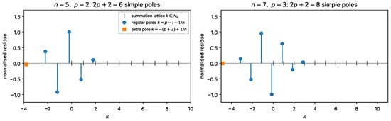
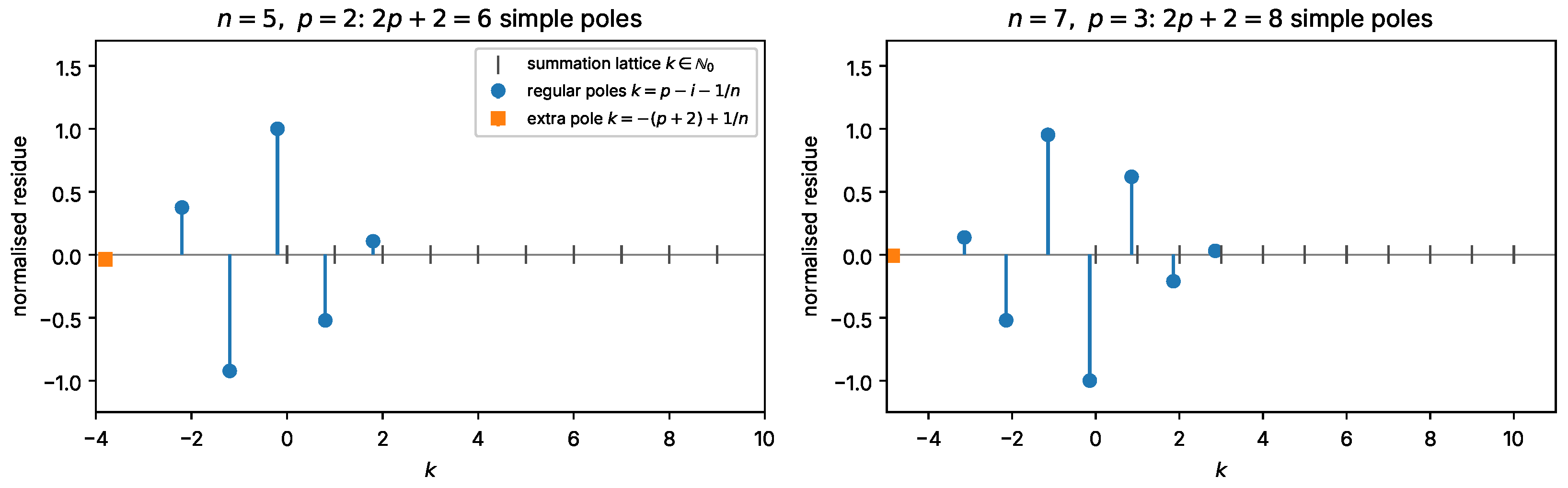
Figure 1 shows the poles of $U_k$ and the normalised residues for $(n,p)=(5,2)$ and $(7,3)$, and Table 3 lists the exact residues for $(n,p)=(5,2)$. Both display the alternating signs of the $a_i$ and the cancellation (49).

Figure 1. Pole–residue structure of the rational kernel (42). The $2p+1$ regular poles $k=p-i-1/n$ are congruent to $-1/n$ modulo 1 and the extra pole $k=-(p+2)+1/n$ to $+1/n$; equivalently, the integers $nk$ at which the denominator factors vanish lie in the residue classes $-1$ and $+1$ modulo n. All poles are simple and none meets the summation lattice $k\in {\mathbb{N}}_0$ (tick marks). Residues are normalised by their largest modulus. The alternating signs, together with the cancellation ${\sum }_i{a}_i=0$ of Proposition 4, are what makes the divergent inner sums arising from (46) combine into a convergent whole (Appendix A).

Table 3. Exact residues (47) and (48) for $(n,p)=(5,2)$, where $K_{5,2}=2376$ and $M(5,2)={\displaystyle \frac{67}{5080320}}$. The six values sum to zero, as required by (49), so the table can be checked by hand.

	${\mathit{a}}_0$	${\mathit{a}}_1$	${\mathit{a}}_2$	${\mathit{a}}_3$	${\mathit{a}}_4$	${\mathit{a}}_5$
value	${\displaystyle \frac{1}{420000}}$	$-{\displaystyle \frac{1}{86250}}$	${\displaystyle \frac{1}{45000}}$	$-{\displaystyle \frac{1}{48750}}$	${\displaystyle \frac{1}{120000}}$	$-{\displaystyle \frac{1}{1205568}}$
pole k	$2-\frac{1}{5}$	$1-\frac{1}{5}$	$-\frac{1}{5}$	$-1-\frac{1}{5}$	$-2-\frac{1}{5}$	$-4+\frac{1}{5}$

4.1. Partial Sums and the Telescoping Constant

The inner sums produced by (46) diverge individually and must be recombined before the limit is taken. We state the outcome; the reindexing is elementary and is carried out in Appendix A.

Definition 1

(Elementary part). For integers $n\ge 2$ and $p\ge 1$ set

$$M(n,p)=-{\displaystyle \sum _{i=p}^{2p}}{a}_i{\displaystyle \sum _{t=0}^{i-p-1}}{\displaystyle \frac{1}{1+nt}}+{\displaystyle \sum _{i=0}^{p-1}}{a}_i{\displaystyle \sum _{t=1}^{p-i}}{\displaystyle \frac{1}{1-nt}}-a_{2p+1}{\displaystyle \sum _{t=0}^p}{\displaystyle \frac{1}{(n-1)+nt}},$$

(50)

with $a_i=a_i(n,p)$ given by (47)–(48); empty sums are 0, so that the index $i=p$ of the first sum contributes nothing. Thus $M(n,p)$ is an explicit rational number.

Definition 2

(Telescoping sums). For $s\in {\mathbb{N}}_0$ and $n\ge 2$ put

$$T_s^{\left(n\right)}={\displaystyle \sum _{k=0}^s}\left({\displaystyle \frac{1}{1+nk}}-{\displaystyle \frac{1}{(n-1)+nk}}\right),T_n=\underset{s\to \infty }{\lim }{T}_s^{\left(n\right)},$$

(51)

the limit existing because the summand is $\mathcal{O}\left(k^{-2}\right)$.

Proposition 5

(Partial-sum decomposition). Let $n\ge 2$, $p\ge 1$, $N\ge 2p$, and $S_N={\sum }_{k=0}^N{U}_k$. Then

$$S_N=M(n,p)-a_{2p+1}{T}_{N-p-1}^{\left(n\right)}+E_N,$$

(52)

where the boundary remainder satisfies

$$|E_N|\le {\displaystyle \frac{(2p+1){\sum }_{i=0}^{2p}\left|a_i\right|}{1+n(N-p)}}+{\displaystyle \frac{(2p+2)|a_{2p+1}|}{n(N-p)+(n-1)}}\underset{N\to \infty }{\to }0.$$

(53)

Proof. 

See Appendix A.   □

Theorem 4

(Closed form of the telescoping constant). For every integer $n\ge 2$,

$$T_n={\int }_0^1{\displaystyle \frac{1-x^{n-2}}{1-x^n}}dx={\displaystyle \frac{1}{n}}\left[\psi \left(\frac{n-1}{n}\right)-\psi \left(\frac{1}{n}\right)\right]={\displaystyle \frac{\pi }{n}}\cot \left({\displaystyle \frac{\pi }{n}}\right).$$

(54)

In particular, $T_2=0$ and

$$T_3={\displaystyle \frac{\pi }{3}}\cot \left({\displaystyle \frac{\pi }{3}}\right)={\displaystyle \frac{\pi }{3\sqrt{3}}}.$$

Proof. 

For $c>0$ and $k\in {\mathbb{N}}_0$, one has

$${\displaystyle \frac{1}{c+nk}}={\int }_0^1{x}^{c-1+nk}dx;$$

with $c=1$ and $c=n-1$, this gives

$${\displaystyle \frac{1}{1+nk}}-{\displaystyle \frac{1}{(n-1)+nk}}={\int }_0^1{x}^{nk}\left(1-x^{n-2}\right)dx.$$

Summing over $k\ge 0$ and interchanging by monotone convergence on $[0,1)$, where ${\sum }_k{x}^{nk}={(1-x^n)}^{-1}$ and $1-x^{n-2}\ge 0$, gives the integral formula. Writing

$$T_n={\displaystyle \frac{1}{n}}\sum _{k\ge 0}\left[{(k+\frac{1}{n})}^{-1}-{(k+\frac{n-1}{n})}^{-1}\right]$$

and using

$$\sum _{k\ge 0}\left[{(k+q)}^{-1}-{(k+q^{\prime })}^{-1}\right]=\psi \left(q^{\prime }\right)-\psi \left(q\right)$$

gives the second expression, and the reflection formula (18) with $z=1/n$, together with ${\displaystyle \frac{n-1}{n}}=1-{\displaystyle \frac{1}{n}}$, gives the third.   □

Remark 8

(Elementary check at $n=3$). For $n=3$, the integrand is

$${\displaystyle \frac{1-x}{1-x^3}}={\displaystyle \frac{1}{x^2+x+1}}$$

and

$$T_3={\int }_0^1{\displaystyle \frac{dx}{{\left(x+\frac{1}{2}\right)}^2+{\left(\frac{\sqrt{3}}{2}\right)}^2}}={\displaystyle \frac{2}{\sqrt{3}}}{\left[\arctan \left({\displaystyle \frac{2x+1}{\sqrt{3}}}\right)\right]}_0^1={\displaystyle \frac{2}{\sqrt{3}}}\left({\displaystyle \frac{\pi }{3}}-{\displaystyle \frac{\pi }{6}}\right)={\displaystyle \frac{\pi }{3\sqrt{3}}},$$

in agreement with (54).

4.2. The Master Evaluation

Combining the partial-sum decomposition with the closed form of $T_n$ gives the value of ${\sum }_k{U}_k$, and hence of $F(n,p)$.

Theorem 5

(Master evaluation). For all integers $n\ge 2$ and $p\ge 1$,

$${\displaystyle \sum _{k=0}^{\infty }}{U}_k=M(n,p)-a_{2p+1}{T}_n=M(n,p)-a_{2p+1}{\displaystyle \frac{\pi }{n}}\cot \left({\displaystyle \frac{\pi }{n}}\right).$$

(55)

Proof. 

By Proposition 5, $S_N=M(n,p)-a_{2p+1}{T}_{N-p-1}^{\left(n\right)}+E_N$ with $E_N\to 0$. Letting $N\to \infty$ and using

$$T_{N-p-1}^{\left(n\right)}\to T_n={\displaystyle \frac{\pi }{n}}\cot \left({\displaystyle \frac{\pi }{n}}\right)$$

(Definition 2 and Theorem 4) gives (55); absolute convergence of ${\sum }_k{U}_k$ is Lemma 5.   □

Theorem 6

(Main closed form). Let $n\ge 2$ and $p\ge 1$ be integers and let $\alpha ,\beta$ be given by (10). Then

$$\begin{array}{cc}\hfill F(n,p)& ={}_{3}F_2\left(1-\alpha ,1,1+\alpha ;1+\alpha -\beta ,\alpha +2;1\right)\hfill \\ \hfill & =(\alpha +1)n{K}_{n,p}\left[M(n,p)-a_{2p+1}{\displaystyle \frac{\pi }{n}}\cot \left({\displaystyle \frac{\pi }{n}}\right)\right],\hfill \end{array}$$

(56)

with $K_{n,p}$, $M(n,p)$ and $a_{2p+1}$ given by (43), (50) and (48).

Proof. 

By Lemma 3, $S=n{K}_{n,p}{\sum }_{k\ge 0}{U}_k$; insert (55) and apply Proposition 2, whose hypotheses hold since $\alpha =p+1-{\displaystyle \frac{1}{n}}>0$, $1+\alpha -\beta >0$ and $2\alpha -\beta =2p+1>0$.   □

Corollary 2

(Digamma form). Under the hypotheses of Theorem 6,

$$F(n,p)=-(\alpha +1)K_{n,p}\left[{\displaystyle \sum _{i=0}^{2p}}{a}_i\psi \left(i-p+{\displaystyle \frac{1}{n}}\right)+a_{2p+1}\psi \left(p+2-{\displaystyle \frac{1}{n}}\right)\right].$$

(57)

Proof. 

Write ${\varrho }_i=i-p+{\displaystyle \frac{1}{n}}$ and ${\varrho }_{*}=p+2-{\displaystyle \frac{1}{n}}$, none of which is a non-positive integer by Lemma 5. Then

$$U_k={\displaystyle \frac{1}{n}}\left[\sum _i{\displaystyle \frac{a_i}{k+{\varrho }_i}}+{\displaystyle \frac{a_{2p+1}}{k+{\varrho }_{*}}}\right],$$

and summing with (17) exactly as in the proof of Theorem 1—the $\log \left(N\right)$ terms cancelling by (49)—gives

$$\sum _{k\ge 0}{U}_k=-{\displaystyle \frac{1}{n}}\left[\sum _i{a}_i\psi \left({\varrho }_i\right)+a_{2p+1}\psi \left({\varrho }_{*}\right)\right].$$

Multiplying by $(\alpha +1)n{K}_{n,p}$ gives (57). Equivalently, (57) is Corollary 1 under the identification (12), whose hypothesis (6) holds for every $n\ge 2$ by Remark 2.   □

Remark 9

(Two routes, one result). Corollary 2 follows both from Theorem 1 and from the kernel analysis of this section; the two derivations are logically independent, and their agreement checks the bookkeeping of Appendix A. The elementary form (56) is the sharper statement: it exhibits the value as a rational number plus a rational multiple of $\pi \cot (\pi /n)$, which (57) does not make visible. The reason the collapse occurs is recorded in Lemma 5: modulo 1 the arguments ${\varrho }_i$ are all congruent to ${\displaystyle \frac{1}{n}}$ and ${\varrho }_{*}$ to $1-{\displaystyle \frac{1}{n}}$, so the differences $\psi \left({\varrho }_i\right)-\psi \left({\varrho }_{i^{\prime }}\right)$ telescope into finite rational sums and only the single reflection pair $\psi (1-{\displaystyle \frac{1}{n}})-\psi \left({\displaystyle \frac{1}{n}}\right)$ survives.

5. Consequences: Transcendence, Special Cases and Limit

This section draws the consequences of Theorem 6: the arithmetic nature of $F(n,p)$, explicit formulas for small p, the endpoint $n=2$, and the limit $n\to \infty$ together with its rate. Throughout what follows, $R(n,p)$ and $C(n,p)$ denote the two rational numbers defined in (59) below—the Rational Part and the cotangent coefficient of $F(n,p)$—and no other meaning is attached to these symbols.

Corollary 3

(Arithmetic nature of the values). For integers $n\ge 2$, $p\ge 1$ there exist $R(n,p),C(n,p)\in \mathbb{Q}$ with $C(n,p)\ne 0$ such that

$$F(n,p)=R(n,p)+C(n,p)\pi \cot \left({\displaystyle \frac{\pi }{n}}\right),$$

(58)

where

$$R(n,p)=(\alpha +1)n{K}_{n,p}M(n,p),C(n,p)=-(\alpha +1)K_{n,p}{a}_{2p+1}.$$

(59)

Consequently, $F(n,p)$ is transcendental for every $n\ge 3$ and rational for $n=2$.

Proof. 

Rationality of R and C is clear from (43), (47), (48) and (50) and $\alpha +1=p+2-{\displaystyle \frac{1}{n}}\in \mathbb{Q}$, and for $C\ne 0$ because $\alpha +1$, $K_{n,p}$ and $a_{2p+1}$ are all non-zero: indeed $\alpha +1>0$; each factor $1-n^2{s}^2$ of $K_{n,p}$ in (43) satisfies $1-n^2{s}^2\le -3$, so that $\mathrm{sign}{K}_{n,p}={(-1)}^p$; and each factor $(2np+2n-2)-nj$ of the denominator in (48) is at least $2n-2\ge 2$ (proof of Proposition 4), so that $a_{2p+1}<0$. Hence $\mathrm{sign}C(n,p)={(-1)}^p$ for all integers $n\ge 2$, $p\ge 1$, in agreement with Table 4.

Table 4. The rational data of (58) for $p=1,2,3$, so that $F(n,p)=R(n,p)+C(n,p)\pi \cot (\pi /n)$. Each entry is a rational function of n in lowest terms; all were checked against direct summation of the defining ${}_{3}F_2\left(1\right)$ at high precision for $2\le n\le 20$, and derived symbolically from (59).

p	$\mathit{R}(\mathit{n},\mathit{p})$ and $\mathit{C}(\mathit{n},\mathit{p})$
1	$R={\displaystyle \frac{(n+1)(3n-1)\left(4n^2-7n+2\right)}{4n(n-1){(2n-1)}^2}}$,   $C=-{\displaystyle \frac{(n+1)(3n-1)}{4n(2n-1)(3n-2)}}$
2	$R={\displaystyle \frac{(2n+1)(4n-1)\left(15n^3-31n^2+22n-4\right)}{12n(n-1)(2n-1){(3n-1)}^2}}$
	$C={\displaystyle \frac{(n+1)(2n+1)(4n-1)}{8n(3n-2)(3n-1)(5n-2)}}$
3	$R={\displaystyle \frac{(3n+1)(5n-1)\left(432n^4-922n^3+673n^2-227n+26\right)}{120n(n-1)(2n-1)(3n-1){(4n-1)}^2}}$
	$C=-{\displaystyle \frac{(n+1)(2n+1)(3n+1)(5n-1)}{16n(3n-2)(4n-1)(5n-2)(7n-2)}}$

Let $n\ge 3$ and put $\zeta =e^{2\pi i/n}$, an algebraic number since ${\zeta }^n=1$, with $\zeta \ne 1$. From 

$$\cot \left(\theta \right)=i(e^{2i\theta }+1)/(e^{2i\theta }-1)$$

with $\theta =\pi /n$,

$$\cot \left({\displaystyle \frac{\pi }{n}}\right)=i{\displaystyle \frac{\zeta +1}{\zeta -1}},$$

(60)

so $\cot (\pi /n)$ is algebraic; and $0<\pi /n\le \pi /3<\pi /2$ gives $\cot (\pi /n)>0$, so it is a non-zero algebraic number. By Lindemann’s theorem ([39], Ch. 1) the number $\pi$ is transcendental, hence, so is $C\cot (\pi /n)·\pi$, a non-zero algebraic multiple of $\pi$; and adding the rational number R preserves transcendence. (Only the transcendence of $\pi$ is used; the full strength of the Lindemann–Weierstrass theorem is not needed.) For $n=2$ one has $\cot (\pi /2)=0$, so $F(2,p)=R(2,p)\in \mathbb{Q}$.   □

5.1. Closed Forms for Small p

For fixed p the quantities $R(n,p)$ and $C(n,p)$ of (59) are rational functions of n, which can be obtained by evaluating (59) symbolically; Table 4 records them for $p=1,2,3$, and Example 3 writes out the case $p=1$.

Example 3

(The case $p=1$). For $p=1$ one has $\alpha =2-{\displaystyle \frac{1}{n}}$, $\beta =1-{\displaystyle \frac{2}{n}}$ and

$$\begin{array}{cc}\hfill {}_{3}F_2\left(\frac{1}{n}-1,1,3-\frac{1}{n};2+\frac{1}{n},4-\frac{1}{n};1\right)& ={\displaystyle \frac{(n+1)(3n-1)(4n^2-7n+2)}{4n(n-1){(2n-1)}^2}}\hfill \\ \hfill & -{\displaystyle \frac{(n+1)(3n-1)}{4n(2n-1)(3n-2)}}\pi \cot \left({\displaystyle \frac{\pi }{n}}\right).\hfill \end{array}$$

At $n=3$, this reads

$$\begin{array}{cc}\hfill {}_{3}F_2\left(-\frac{2}{3},1,\frac{8}{3};\frac{7}{3},\frac{11}{3};1\right)& ={\displaystyle \frac{68}{75}}-{\displaystyle \frac{8}{105}}\pi \cot \left({\displaystyle \frac{\pi }{3}}\right)={\displaystyle \frac{68}{75}}-{\displaystyle \frac{8\pi }{105\sqrt{3}}}\hfill \\ \hfill & =0.768472429391678639954\dots ,\hfill \end{array}$$

and at $n=4$ since $\cot (\pi /4)=1$,

$${\displaystyle \frac{1045}{1176}}-{\displaystyle \frac{11}{224}}\pi =0.734330802938086258910\dots$$

5.2. The Endpoint $n=2$

At $n=2$, the cotangent term vanishes and the series reduces to a Gauss series, which gives an independent check of the closed form.

Proposition 6

(Gauss-summable endpoint). For $n=2$, one has $\beta =0$, $\alpha =p+{\displaystyle \frac{1}{2}}$, the ${}_{3}F_2$ collapses to a Gauss function, and 

$$F(2,p)={}_{2}F_1\left(1-\alpha ,1;\alpha +2;1\right)={\displaystyle \frac{\alpha +1}{2\alpha }}={\displaystyle \frac{2p+3}{2(2p+1)}}\in \mathbb{Q},$$

(61)

in agreement with Theorem 6 and Corollary 3, because $T_2={\displaystyle \frac{\pi }{2}}\cot \left({\displaystyle \frac{\pi }{2}}\right)=0$.

Proof. 

At $n=2$, the first lower parameter is $1+\alpha -\beta =1+\alpha$, which cancels the upper parameter $1+\alpha$; the series reduces to ${}_{2}F_1(1-\alpha ,1;\alpha +2;1)$, summed by Gauss’s theorem as

$$\Gamma (\alpha +2)\Gamma \left(2\alpha \right)/[\Gamma (2\alpha +1)\Gamma (\alpha +1)]={\displaystyle \frac{\alpha +1}{2\alpha }}.$$

On the other hand, $T_2=0$ by Theorem 4, so (56) returns the rational number $2(\alpha +1)K_{2,p}M(2,p)$. Since Theorem 6 holds at $n=2$, this number equals (61); no computation is needed for this conclusion, and exact arithmetic for $1\le p\le 12$ confirms it independently (Section 6).   □

This endpoint is a useful independent check: it is the only member of the family for which a classical summation theorem applies directly, and the general formula reproduces it with the transcendental term switched off.

5.3. The Limit $n\to \infty$

We now let $n\to \infty$ with p fixed; the lattice parameters then tend to integers and the series becomes terminating.

Proposition 7

(Terminating limit). For each fixed $p\ge 1$,

$$\underset{n\to \infty }{\lim }F(n,p)={}_{3}F_2\left(-p,1,p+2;p+1,p+3;1\right),$$

(62)

a terminating series with rational value.

Proof. 

As $n\to \infty$ we have $\alpha \to p+1$ and $\beta \to 1$, so for each fixed k the k-th term $t_k=t_k\left(n\right)$ of (11) converges to the k-th term of the right-hand side of (62); since ${\left(1-\alpha \right)}_k\to {\left(-p\right)}_k=0$ for $k>p$, only the indices $k\le p$ survive in the limit.

The passage to the limit term by term is justified by dominated convergence with respect to counting measure, using the explicit dominating sequence supplied by Lemma 4: put

$${\omega }_k=\left\{\begin{array}{cc}1,\hfill & 0\le k\le 2p,\hfill \\ (p+2){(2p+1)}^{2p+1}{k}^{-(2p+2)},\hfill & k\ge 2p+1.\hfill \end{array}\right.$$

By parts (i) and (ii) of that lemma, $|t_k\left(n\right)|\le {\omega }_k$ for every $k\in {\mathbb{N}}_0$ and every integer $n\ge 2$, the bound being uniform in n; ${\sum }_k{\omega }_k<\infty$ because $2p+2\ge 4$. Hence

$$\underset{n\to \infty }{\lim }\sum _k{t}_k\left(n\right)=\sum _k\underset{n\to \infty }{\lim }{t}_k\left(n\right),$$

which is (62).   □

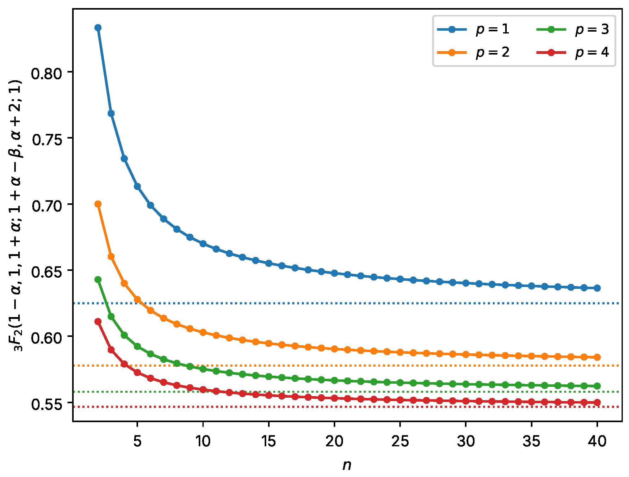
The limits for the first few p are listed in Table 5. The transcendental term does not disappear in the limit: since

$${\displaystyle \frac{\pi }{n}}\cot \left({\displaystyle \frac{\pi }{n}}\right)\to 1$$

and

$$C(n,p)\pi \cot \left({\displaystyle \frac{\pi }{n}}\right)=nC(n,p)·{\displaystyle \frac{\pi }{n}}\cot \left({\displaystyle \frac{\pi }{n}}\right)$$

with $nC(n,p)$ tending to a non-zero rational limit, it is the balance between the two parts of (58) that produces the rational value. For $p=1$, for instance, $R(n,1)\to {\displaystyle \frac{3}{4}}$ and $nC(n,1)\to -{\displaystyle \frac{1}{8}}$, reproducing ${\displaystyle \frac{3}{4}}-{\displaystyle \frac{1}{8}}={\displaystyle \frac{5}{8}}$.

Table 5. The limits $L_p$ of (62), computed from the terminating series, and the coefficients $c_p$ of the $n^{-1}$ term in Proposition 8, so that $F(n,p)=L_p+c_p/n+\mathcal{O}\left(n^{-2}\right)$. The limits were confirmed numerically from Theorem 6 at $n={10}^5$, and the coefficients by checking that $\left(F(n,p)-L_p\right)n/c_p\to 1$.

p	1	2	3	v4	5	6
$L_p$	${\displaystyle \frac{5}{8}}$	${\displaystyle \frac{26}{45}}$	${\displaystyle \frac{125}{224}}$	${\displaystyle \frac{41}{75}}$	${\displaystyle \frac{427}{792}}$	${\displaystyle \frac{340}{637}}$
$c_p$	${\displaystyle \frac{11}{24}}$	${\displaystyle \frac{19}{75}}$	${\displaystyle \frac{2029}{11760}}$	${\displaystyle \frac{34421}{264600}}$	${\displaystyle \frac{6857377}{65862720}}$	${\displaystyle \frac{46888187}{541080540}}$
decimal $L_p$	$0.6250$	$0.5778$	$0.5580$	$0.5467$	$0.5391$	$0.5338$

The same decomposition fixes the rate at which the limit is approached.

Proposition 8

(Rate of approach). Fix $p\ge 1$ and let $L_p$ denote the limit (62). Then $R(n,p)$ and $C(n,p)$ are rational functions of n, the function $nC(n,p)$ is bounded, and

$$F(n,p)=\left[R(n,p)+nC(n,p)\right]+\mathcal{O}\left(n^{-2}\right)=L_p+{\displaystyle \frac{c_p}{n}}+\mathcal{O}\left(n^{-2}\right)(n\to \infty ),$$

(63)

where $c_p\in \mathbb{Q}$ is the coefficient of $n^{-1}$ in the expansion of $R(n,p)+nC(n,p)$ at $n=\infty$. In particular the approach is $\mathcal{O}\left(n^{-1}\right)$, and $\Theta \left(n^{-1}\right)$ whenever $c_p\ne 0$; for $p=1,\dots ,6$,

$$c_p={\displaystyle \frac{11}{24}},{\displaystyle \frac{19}{75}},{\displaystyle \frac{2029}{11760}},{\displaystyle \frac{34421}{264600}},{\displaystyle \frac{6857377}{65862720}},{\displaystyle \frac{46888187}{541080540}}$$

(Table 5), all positive, so that for these p, $F(n,p)>L_p$ for all sufficiently large n. (Direct evaluation shows that in fact $F(n,p)>L_p$ for $2\le n\le 400$, $1\le p\le 6$.)

Proof. 

By (43), (47), (48) and (50), each of $a_i$, $K_{n,p}$ and $M(n,p)$ is a finite sum of products of rational functions of n; hence, so are R and C in (58). Moreover

$$|K_{n,p}|={\displaystyle \prod _{s=1}^p}(n^2{s}^2-1)=\Theta \left(n^{2p}\right)$$

and

$$|a_{2p+1}|={\displaystyle \prod _{j=0}^{2p}}{\left(n(2p+2-j)-2\right)}^{-1}=\Theta \left(n^{-(2p+1)}\right),$$

while $\alpha +1=\Theta \left(1\right)$, so $C(n,p)=\Theta \left(n^{-1}\right)$ and $nC(n,p)$ is bounded.

Put $g\left(x\right)=x\cot \left(x\right)$, which is analytic at $x=0$ with $g\left(0\right)=1$ and

$$g\left(x\right)=1-{\displaystyle \frac{x^2}{3}}+\mathcal{O}\left(x^4\right).$$

Since

$$C\pi \cot \left({\displaystyle \frac{\pi }{n}}\right)=nC·g\left({\displaystyle \frac{\pi }{n}}\right),$$

$$F(n,p)=R+nC+nC\left[g\left({\displaystyle \frac{\pi }{n}}\right)-1\right]=R+nC+\mathcal{O}\left(n^{-2}\right),$$

the error term because $nC$ is bounded and $g(\pi /n)-1=\mathcal{O}\left(n^{-2}\right)$. The function $R+nC$ is a rational function of n, so it admits an asymptotic expansion in powers of $n^{-1}$ at $n=\infty$; its limit is $L_p$ by Proposition 7 and the display above, which gives (63). The listed values of $c_p$ are obtained by expanding $R+nC$ symbolically.   □

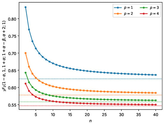
Figure 2 shows the convergence. The curves are visibly monotone in n; we have not proved monotonicity and state it only as an observation, whereas the limits and the $\Theta \left(n^{-1}\right)$ rate that the figure also displays are Propositions 7 and 8.

Figure 2. The value $F(n,p)$ of (11) as a function of n for $p=1,2,3,4$, evaluated from Theorem 6. The dotted lines are the terminating limits $L_p$ of Proposition 7; the gap $F(n,p)-L_p$ decays like $c_p/n$ with $c_p>0$ by Proposition 8; over the plotted range each curve lies above its limit, as checked directly. The leftmost point of each curve is the rational Gauss-summable value (61) at $n=2$; every other point is transcendental by Corollary 3. The apparent monotonicity in n is an observation, not a proved statement.

6. Numerical Verification

The computations reported in this section complement the proofs; they do not replace any of them. Every result of Section 2, Section 3, Section 4 and Section 5 is proved analytically, and no step of any proof uses a numerical value. The computations serve three purposes: they guard against slips of sign and index in the long finite sums, which a proof read on paper can easily miss; they illustrate the statements in concrete cases; and they quantify the practical advantage of the closed form over direct summation of the series. A failed check would point to an error in a specific proof, whereas a successful check is evidence of correct bookkeeping, not a substitute for the argument. All computations were carried out in Python 3.13.16 with mpmath at 60 decimal digits and, for every rational quantity, in exact rational arithmetic; the scripts are listed under Supplementary Materials. An independent computational implementation was used to cross-check the reported numerical values; the scope of these checks is described in Section 6.2.

6.1. Agreement with Independent Evaluations

Table 6 compares four separately implemented evaluation routes: the defining ${}_{3}F_2\left(1\right)$ summed directly; the elementary form (56); the digamma form (57); and the general formula (8) specialised through (12). Formula (8) was in addition checked at 200 randomly drawn non-lattice parameter pairs $(b,c)$, real and complex, with $0\le m,r\le 8$; at the three structurally distinct configurations $m=r=0$, $(m,r)=(1,0)$ and a genuinely two-sided case $(m,r)=(3,2)$; and, for Theorem 3, at $q=1,2,3,4$.

Table 6. High-precision verification. Column $F(n,p)$ gives the value of (11) to 25 significant digits; the last three columns give the relative deviation from direct summation of the elementary form (56), the digamma form (57) and the general formula (8), at 60-digit working precision.

n	p	$\mathit{F}(\mathit{n},\mathit{p})$	Elementary	Digamma	General
3	1	$0.7684724293916786399547369$	0	$2.0·{10}^{-61}$	$2.0·{10}^{-61}$
3	2	$0.6602726383652399514260708$	$1.2·{10}^{-61}$	$1.2·{10}^{-61}$	$1.2·{10}^{-61}$
3	5	$0.5737200102292949433004084$	0	$1.4·{10}^{-61}$	0
4	1	$0.7343308029380862589105292$	$1.1·{10}^{-61}$	0	0
4	3	$0.6008172967641788405688512$	0	$1.3·{10}^{-61}$	$1.3·{10}^{-61}$
5	2	$0.6277493973793652413900444$	$1.2·{10}^{-61}$	$3.7·{10}^{-61}$	$1.2·{10}^{-61}$
5	6	$0.5510588668193711767374259$	0	$1.4·{10}^{-61}$	0
6	4	$0.5682836484453750531969945$	0	$1.4·{10}^{-61}$	$1.4·{10}^{-61}$
7	1	$0.6887515889040630341267620$	0	0	$1.1·{10}^{-61}$
7	8	$0.5357521231047342341754585$	0	0	$1.5·{10}^{-61}$
9	3	$0.5771376225501132163511481$	0	$1.3·{10}^{-61}$	$2.7·{10}^{-61}$
10	5	$0.5495418961432266180384789$	$1.4·{10}^{-61}$	$5.7·{10}^{-61}$	$1.4·{10}^{-61}$
12	2	$0.5987691806126100337611815$	0	$3.9·{10}^{-61}$	0
15	7	$0.5346287791432531910637358$	$1.5·{10}^{-61}$	$5.8·{10}^{-61}$	$1.5·{10}^{-61}$
20	10	$0.5244218526860830436503490$	0	$8.9·{10}^{-61}$	$1.5·{10}^{-61}$

The four routes share the parameter conventions and the basic Pochhammer routine, which are therefore not tested by Table 6; they do not share the mathematics under test. Direct summation uses only (1); the digamma form uses the residues of Proposition 4 but not $T_n$; the elementary form uses the residues, the reindexing of Appendix A and Theorem 4; and (8) uses none of the lattice machinery. A disagreement would therefore localise an error. Two exact identities are worth running before any floating-point comparison, since they either hold or fail outright: the residues must satisfy ${\sum }_{i=0}^{2p+1}{a}_i=0$, and at $n=2$ the closed form must return the rational number (61) with no cotangent contribution.

6.2. Independent Computational Cross-Checks

An implementation developed separately from the primary verification scripts was used to cross-check the formulas and numerical values. Theorems 1, 2 and 3 were checked against direct summation at random real and complex parameters (relative deviations below ${10}^{-20}$ at 30-digit working precision, the limit being the accuracy of the series acceleration); the closed forms of Remark 1 and the cancellation identities (9) and (33) were confirmed; Proposition 1 was confirmed by evaluating (26) at $a=1-{10}^{-30}$ in 80-digit arithmetic, where the two terms cancel to about 30 digits and their sum differs from (8) by a relative amount below ${10}^{-30}$, that is, of the order of $\delta$, as (27) predicts; Table 4 and the values $L_p$, $c_p$ of Table 5 were re-derived symbolically; the endpoint (61) was confirmed in exact arithmetic for $1\le p\le 12$; and all fifteen rows of Table 6 were reproduced. The independent computations provide cross-checks of symbolic reductions, special cases and the accuracy of the numerical evaluation routes. Numerical agreement complements, but does not replace, the analytical proofs.

6.3. Rate of Convergence of the Defining Series

The exact expression (45) permits a sharp determination of the truncation error, not merely an upper bound.

Theorem 7

(Truncation rate). Fix integers $n\ge 2$, $p\ge 1$ and put

$$A(n,p)=(\alpha +1){\left(1-\alpha \right)}_{2p+1}=(\alpha +1){\displaystyle \frac{K_{n,p}}{n^{2p+1}}}\ne 0.$$

(64)

With $t_k$ the terms of (11):

(i) 

$t_k\sim A(n,p)k^{-(2p+2)}$ as $k\to \infty$;

(ii) 

$\mathrm{sign}{t}_k=\mathrm{sign}A(n,p)={(-1)}^p$ for every $k\ge p$;

(iii) 

as $N\to \infty$,

$$\sum _{k>N}{t}_k\sim {\displaystyle \frac{A(n,p)}{2p+1}}{N}^{-(2p+1)},\mathit{so}\mathit{that}\left|\sum _{k>N}{t}_k\right|=\Theta \left(N^{-(2p+1)}\right).$$

The constants implicit in ∼ and Θ depend on n and p, which are fixed throughout. Consequently, attaining relative accuracy ε by direct summation (the partial sums of the defining series, without acceleration) requires $\Theta \left({\epsilon }^{-1/(2p+1)}\right)$ terms.

Proof. 

(i) By (45),

$$t_k=A(n,p)/\left[{\left(k+1-\alpha \right)}_{2p+1}(k+\alpha +1)\right],$$

and the denominator is a monic polynomial in k of degree $2p+2$; hence $k^{2p+2}{t}_k\to A(n,p)$. That $A(n,p)\ne 0$ follows from $K_{n,p}\ne 0$ in (43).

(ii) Write $u=1/n\in (0,\frac{1}{2}]$. For $k\ge p$ every factor of ${\prod }_{s=k-p}^{k+p}(s+u)$ satisfies $s+u\ge u>0$, and $k+\alpha +1>0$, so by (45) the sign of $t_k$ is that of ${\prod }_{s=-p}^p(s+u)$. Exactly the p factors with $s=-1,\dots ,-p$ are negative, because $0<u<1$; hence that sign is ${(-1)}^p$, which is also the sign of $A(n,p)$.

(iii) All the estimates of this part are stated for the modulus of the tail; the sign is restored at the end from (ii). Note first that, by (ii), the terms $t_k$ with $k\ge p$ all have the sign of A, so for $N\ge p$

$$\left|\sum _{k>N}{t}_k\right|=\sum _{k>N}\left|t_k\right|.$$

(65)

Let $\epsilon \in (0,1)$. By (i) there is $k_{\epsilon }\ge p$ with

$$(1-\epsilon )\left|A\right|k^{-(2p+2)}\le |t_k|\le (1+\epsilon )|A|k^{-(2p+2)}(k\ge k_{\epsilon }),$$

so that, summing over $k>N$ and using (65), for $N\ge k_{\epsilon }$

$$(1-\epsilon )\left|A\right|\sum _{k>N}{k}^{-(2p+2)}\le \left|\sum _{k>N}{t}_k\right|\le (1+\epsilon )\left|A\right|\sum _{k>N}{k}^{-(2p+2)}.$$

All three members are non-negative, as they must be.

Comparison with ${\int }_N^{\infty }{x}^{-(2p+2)}dx$ on each unit interval gives

$${\displaystyle \frac{N^{-(2p+1)}}{2p+1}}-{\displaystyle \frac{1}{N^{2p+2}}}\le \sum _{k>N}{k}^{-(2p+2)}\le {\displaystyle \frac{N^{-(2p+1)}}{2p+1}},$$

so

$$\sum _{k>N}{k}^{-(2p+2)}\sim N^{-(2p+1)}/(2p+1).$$

Applying lim sup and lim inf to the modulus therefore yields

$$\underset{N\to \infty }{\mathrm{lim\; sup}}{N}^{2p+1}\left|\sum _{k>N}{t}_k\right|\le {\displaystyle \frac{(1+\epsilon )\left|A\right|}{2p+1}},\underset{N\to \infty }{\mathrm{lim\; inf}}{N}^{2p+1}\left|\sum _{k>N}{t}_k\right|\ge {\displaystyle \frac{(1-\epsilon )\left|A\right|}{2p+1}},$$

for every $\epsilon \in (0,1)$; letting $\epsilon \to 0$ gives

$$\left|\sum _{k>N}{t}_k\right|\sim {\displaystyle \frac{\left|A\right(n,p\left)\right|}{2p+1}}{N}^{-(2p+1)}.$$

(66)

Finally, by (ii), the tail carries the sign of $A(n,p)$ for $N\ge p$, so (66) may be de-absolutised:

$$\sum _{k>N}{t}_k\sim {\displaystyle \frac{A(n,p)}{2p+1}}{N}^{-(2p+1)},$$

which is the assertion. The last statement of the theorem follows because $F(n,p)$ is a fixed non-zero number, so relative and absolute truncation errors have the same order.   □

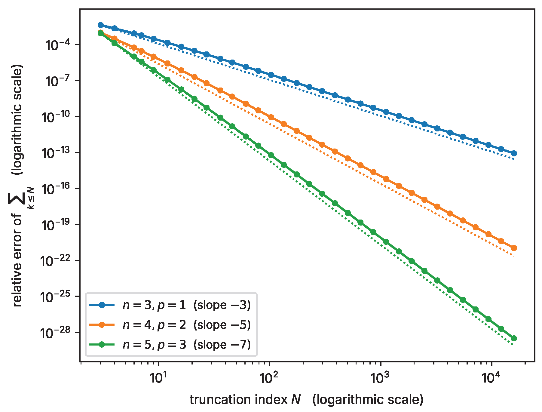
The exponent $2p+2$ in (i) is one more than the parametric excess (15), the extra power coming from the factor $(\alpha +1)/(k+\alpha +1)$ in (45). For small p the cost of direct summation is prohibitive: reaching relative error ${10}^{-15}$ requires summation up to the index N = 69,980 (that is, 69,981 terms) at $(n,p)=(3,1)$ and up to $N=1050$ (1051 terms) at $(3,2)$, whereas Theorem 6 needs $\mathcal{O}\left(p\right)$ operations (Appendix B). Figure 3 measures the truncation error directly and confirms the exponent: the slopes $-3,-5,-7$ of the reference lines are the values $-(2p+1)$ for $p=1,2,3$ predicted by part (iii) of Theorem 7.

Figure 3. Relative error of the truncated series ${\sum }_{k\le N}{t}_k$ for (11), measured against the closed form (56). Both axes are logarithmic: the horizontal axis carries the truncation index N (the partial sum has $N+1$ terms) on a base-10 logarithmic scale and the vertical axis the relative error on the same scale, so that a power law $N^{-\theta }$ appears as a straight line of slope $-\theta$ and the slope can be read off directly. By Theorem 7 the terms decay as $k^{-(2p+2)}$ with a non-zero leading constant and constant sign, so the truncation error decays as $N^{-(2p+1)}$; the dotted reference lines have the corresponding slopes $-3,-5,-7$ for $p=1,2,3$. The closed form is exact at every N by construction, so the plot measures the cost of avoiding it.

6.4. Cost, Conditioning and the Limiting Route

Three computational aspects of the closed form are treated in Appendix B, so as not to interrupt the main line of the paper. In brief: Algorithm A1 evaluates $R(n,p)$, $C(n,p)$ and $F(n,p)$ in $\mathcal{O}\left(p\right)$ arithmetic operations (Proposition A1); the closed form is well conditioned in the tested range, at most about $1.3$ decimal digits being lost to cancellation for $p\le 40$; and the limiting route $a\to 1$ through the formulas of Table 1 cannot deliver more than about half of the working precision, whereas (56) returns R and C exactly.

7. Conclusions

We have obtained a finite digamma evaluation of the unit-numerator family ${}_{3}F_2\left(1,b,c;b+1+m,c+1+r;1\right)$, valid whenever the associated rational kernel has simple poles, that is, whenever $b-c\notin I_{m,r}$ (Theorem 1), and a companion evaluation on the complementary locus, where the poles merge in pairs and one trigamma value appears for each merged pair (Theorem 2); the two together cover all $b,c\in \mathbb{C}\setminus {\mathbb{Z}}_{\le 0}$. Theorem 3 records the ${}_{q+1}F_q\left(1\right)$ analogue under the corresponding pairwise pole-separation condition. Proposition 1 computes the finite part of the Shpot–Srivastava formula at $a=1$ directly from its expansion in $\delta =1-a$ and recovers the same expression, so the formula is identified as the regularization of ([2], Equation (31)), carrying out the limiting analysis left open in ([2], Remark 3).

On the lattice $\alpha =p+1-1/n$, $\beta =1-2/n$ the $2p+2$ poles of the kernel are congruent to $\pm 1/n$ modulo 1; all but one of the digamma differences then telescope into finite rational sums and the surviving pair is resolved by the reflection formula, so that the value is a rational number plus a rational multiple of $\pi \cot (\pi /n)$ (Theorem 6). The cotangent coefficient is non-zero, which makes $F(n,p)$ transcendental for every $n\ge 3$, while $n=2$ reduces to Gauss’s summation theorem and a rational value (Corollary 3, Proposition 6). Explicit rational functions of n are recorded for $p=1,2,3$, and the limit $n\to \infty$ is a terminating ${}_{3}F_2$.

Of these results, the arithmetic specialization is the principal contribution; the evaluation at $a=1$ supplies the tool that makes it available in closed form, and the numerical work of Section 6 and Appendix B confirms and quantifies, but does not replace, the proofs.

Two directions remain open. The first is arithmetic rather than analytic: on a lattice meeting the confluent locus, Theorem 2 delivers trigamma values at rational arguments, and the analogue of the collapse proved here would require knowing which combinations of such values are elementary—a question of a different nature from the digamma case, where the reflection formula settles it. The second is the general ${}_{q+1}F_q\left(1\right)$ setting: Theorem 3 evaluates it under pairwise pole separation, but poles of order up to q can occur when that hypothesis fails (Remark 6), and characterising which lattices there admit a collapse as complete as the one obtained here is open.

Appendix B.1. Evaluation Cost

Appendix B.1.1. Computational Model

We count arithmetic operations $(+,-,\times ,÷)$ on numbers held in a fixed working precision, each at unit cost, and treat one evaluation of $\pi \cot (\pi /n)$ as $\mathcal{O}\left(1\right)$. The statement below is therefore an operation count for floating-point evaluation; it is not a bit-complexity statement, and we return to that point at the end of the subsection.

The prefix sums of the algorithm are denoted ${\Sigma }_s^{\pm }$, to avoid confusion with the coefficients $P_j$, $Q_j$ of Theorem 2. Read literally, (50) contains nested finite sums totalling $\Theta \left(p^2\right)$ terms, and (47) and (48) contain factorials and a product of $2p+1$ factors. Algorithm A1 removes the nesting by updating the residues by a two-term recurrence and accumulating the inner sums once as prefix sums.

Algorithm A1 Evaluation of $R(n,p)$, $C(n,p)$ and $F(n,p)$

1: $D\leftarrow 2np+2n-2$;   $\alpha \leftarrow p+1-1/n$   2: $a_0\leftarrow {\left[n^{2p}\left(2p\right)!D\right]}^{-1}$      ▹$n^{2p}$ and $\left(2p\right)!$ by running products: $\mathcal{O}\left(p\right)$   3: for $i=0,\dots ,2p-1$ do   4:      $a_{i+1}\leftarrow -a_i·{\displaystyle \frac{2p-i}{i+1}}·{\displaystyle \frac{D-ni}{D-n(i+1)}}$                   ▹ from (47)   5: end for   6: $\mathrm{\Pi }\leftarrow 1$; for $j=0,\dots ,2p$ do $\mathrm{\Pi }\leftarrow \mathrm{\Pi }(D-nj)$;   $a_{2p+1}\leftarrow -1/\mathrm{\Pi }$   7: ${\Sigma }_0^{+}\leftarrow 0$; for $s=0,\dots ,p-1$ do ${\Sigma }_{s+1}^{+}\leftarrow {\Sigma }_s^{+}+{(1+ns)}^{-1}$      ▹${\Sigma }_s^{+}={\sum }_{t=0}^{s-1}{(1+nt)}^{-1}$   8: ${\Sigma }_0^{-}\leftarrow 0$; for $s=1,\dots ,p$ do ${\Sigma }_s^{-}\leftarrow {\Sigma }_{s-1}^{-}+{(1-ns)}^{-1}$   9: $W\leftarrow 0$; for$t=0,\dots ,p$ do $W\leftarrow W+{\left((n-1)+nt\right)}^{-1}$ 10: $M\leftarrow -{\sum }_{i=p}^{2p}{a}_i{\Sigma }_{i-p}^{+}+{\sum }_{i=0}^{p-1}{a}_i{\Sigma }_{p-i}^{-}-a_{2p+1}W$                   ▹ (50) 11: $K\leftarrow 1$; for $s=1,\dots ,p$ do $K\leftarrow K(1-n^2{s}^2)$ 12: $R\leftarrow (\alpha +1)nKM$;   $C\leftarrow -(\alpha +1)K{a}_{2p+1}$ 13: return R, C, and $F=R+C\pi \cot (\pi /n)$

Proposition A1.

In the model above, Algorithm A1 evaluates $R(n,p)$, $C(n,p)$ and $F(n,p)$ in $\mathcal{O}\left(p\right)$ arithmetic operations and $\mathcal{O}\left(p\right)$ storage.

Proof. 

Every loop of Algorithm A1 runs $\mathcal{O}\left(p\right)$ times and performs $\mathcal{O}\left(1\right)$ operations per iteration; the two accumulation sums in line 10 have $p+1$ and p terms, and each summand $a_i{\Sigma }_{i-p}^{+}$ or $a_i{\Sigma }_{p-i}^{-}$ costs one multiplication because the prefix sums ${\Sigma }_s^{\pm }$ were computed once in lines 7–8. Correctness of the recurrence in line 4 is immediate from (47):

$$a_{i+1}/a_i=-{\displaystyle \frac{2p-i}{i+1}}·{\displaystyle \frac{D-ni}{D-n(i+1)}},$$

all denominators being non-zero by Proposition 4. The arrays a, ${\Sigma }^{+}$, ${\Sigma }^{-}$ have $\mathcal{O}\left(p\right)$ entries. □

Direct summation without acceleration, by contrast, needs $\Theta \left({\epsilon }^{-1/(2p+1)}\right)$ terms by Theorem 7, each costing $\mathcal{O}\left(1\right)$ operations through the ratio recurrence for hypergeometric terms; Table S1 of the supplementary archive lists the truncation index needed for a relative error of ${10}^{-15}$, together with $\kappa (n,p)$ of Appendix B.2.

Appendix B.1.2. Bit Complexity

Proposition A1 is not a bit-complexity statement. In exact rational arithmetic the integers occurring in Algorithm A1—$\left(2p\right)!$, $n^{2p}$, ${\prod }_j(D-nj)$ and $K_{n,p}$—have $\Theta \left(p\log \left(np\right)\right)$ bits, and the rational numerators and denominators of $M(n,p)$ grow accordingly. The exact cost is therefore $\mathcal{O}\left(p\right)$ arithmetic operations on operands of $\mathcal{O}\left(p\log \right(np\left)\right)$ bits, that is $\mathcal{O}\left(p\mathsf{M}\left(p\log \right(np\left)\right)\right)$ bit operations, where $\mathsf{M}(\ell )$ denotes the cost of multiplying two ℓ-bit integers. In fixed-precision floating-point arithmetic the operand size is constant and the count is $\mathcal{O}\left(p\right)$ as stated.

Appendix B.2. Conditioning

The residues (47) alternate in sign and $K_{n,p}$ grows rapidly in p, so the numerical behaviour of (56) deserves comment. The relevant quantity is not the size of $K_{n,p}$—it enters multiplicatively and only consumes exponent range—but the cancellation inside the bracket. Writing that bracket as a sum ${\sum }_{\ell }{\tau }_{\ell }$ of the $p(p+1)+p+2$ elementary terms obtained by expanding (50) and appending

$$-a_{2p+1}{\displaystyle \frac{\pi }{n}}\cot \left({\displaystyle \frac{\pi }{n}}\right),$$

define

$$\kappa (n,p)={\displaystyle \frac{{\sum }_{\ell }\left|{\tau }_{\ell }\right|}{\left|{\sum }_{\ell }{\tau }_{\ell }\right|}}\ge 1.$$

(A5)

Here $\kappa$ is a rule-of-thumb condition estimate for the bracket regarded as a sum of given terms, the usual heuristic being that summation in t-digit arithmetic then returns about $t-{\log }_{10}\left(\kappa \right)$ correct digits. It is not a forward error analysis: it ignores the rounding committed in forming the residues, products, prefix sums and cotangent, and says nothing about the backward stability of Algorithm A1. What follows therefore concerns the conditioning of the expression, measured in exact arithmetic; no backward error bound for the algorithm is claimed.

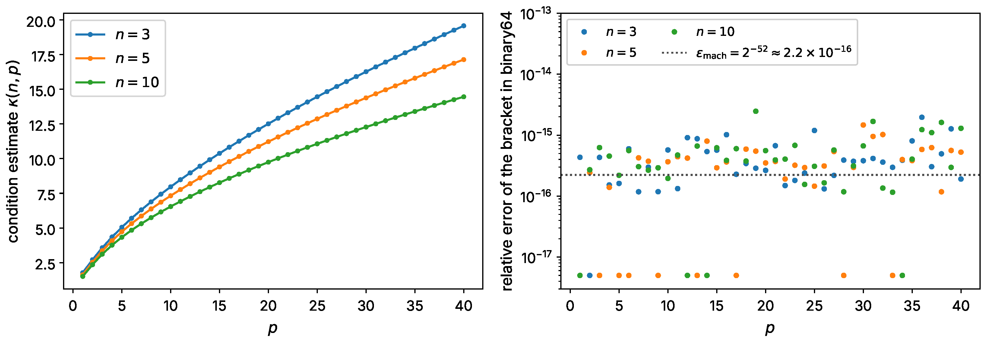
The summation order used in our implementation is the one written in Algorithm A1: recursive (sequential) accumulation in increasing i, with no compensated or pairwise summation, in IEEE-754 binary64 [40], whose unit round-off is $\mathsf{u}=2^{-53}$ (the symbol $\mathsf{u}$ is used here to avoid confusion with $u=1/n$ in Lemma 4). We computed $\kappa (n,p)$ in exact rational arithmetic (the cotangent term in high-precision arithmetic) for $n\in \{3,5,10\}$ and $1\le p\le 40$, and for all $2\le n\le 20$ with $1\le p\le 12$. Over these ranges $\kappa$ increases slowly with p and decreases with n (Figure A1, left), the observed maxima being

$$\underset{\begin{array}{c}2\le n\le 20\\ 1\le p\le 5\end{array}}{\max }\kappa (n,p)=5.08,\underset{\begin{array}{c}2\le n\le 20\\ 1\le p\le 12\end{array}}{\max }\kappa (n,p)=9.12,\underset{\begin{array}{c}n\in \{3,5,10\}\\ 1\le p\le 40\end{array}}{\max }\kappa (n,p)=19.58,$$

each attained at the smallest n and largest p of the corresponding range, so that at most about $1.3$ decimal digits are lost anywhere in the tested range. Evaluating the bracket in binary64 over the same range and comparing with the exact rational value gave relative errors not exceeding $2.5\times {10}^{-15}$, that is, at most about $22\mathsf{u}$; the median is $3.5\times {10}^{-16}$ for $n\in \{3,5,10\}$, $1\le p\le 40$, the range shown in Figure A1, right, and $1.8\times {10}^{-16}$ for $2\le n\le 20$, $1\le p\le 12$. These are empirical observations about the tested implementation, parameter ranges and platform; no uniform bound on $\kappa (n,p)$ over all $(n,p)$ is proved, and none is claimed. The observed growth is compatible with $\kappa =\mathcal{O}\left(\log \right(p\left)\right)$, which we record only as an observation.

Figure A1. (Left): the condition estimate (A5) for the bracket of (56), computed in exact rational arithmetic, stays below 20 for $p\le 40$ at $n=3,5,10$. (Right): relative error of the same bracket evaluated in IEEE-754 binary64 by the summation order of Algorithm A1, measured against the exact rational value; the dotted line marks ${\epsilon }_{\mathrm{mach}}=2^{-52}\approx 2.2\times {10}^{-16}$, and points on the bottom row indicate agreement below $5\times {10}^{-18}$. Both panels report the tested parameter ranges only; neither is a forward error analysis, and no behaviour outside these ranges is claimed.

Figure A1. (Left): the condition estimate (A5) for the bracket of (56), computed in exact rational arithmetic, stays below 20 for $p\le 40$ at $n=3,5,10$. (Right): relative error of the same bracket evaluated in IEEE-754 binary64 by the summation order of Algorithm A1, measured against the exact rational value; the dotted line marks ${\epsilon }_{\mathrm{mach}}=2^{-52}\approx 2.2\times {10}^{-16}$, and points on the bottom row indicate agreement below $5\times {10}^{-18}$. Both panels report the tested parameter ranges only; neither is a forward error analysis, and no behaviour outside these ranges is claimed.

Appendix B.3. Comparison with the Limiting Route

None of the first three formulas of Table 1 returns a number at $a=1$, so a side-by-side comparison of values is impossible; the only comparison those formulas permit is to evaluate at $a=1-\delta$ and let $\delta \to 0$. Doing this for $(n,p)=(3,1)$ with the two terms ${\Phi }_1,{\Phi }_2$ of (26) confirms Proposition 1 in three ways: the two terms grow like ${\delta }^{-1}$ while their sum stays bounded; the error of the sum decreases like $\delta$; and the digits lost to cancellation,

$${\log }_{10}\left(\underset{i}{\max }|{\Phi }_i|/|{\Phi }_1+{\Phi }_2|\right),$$

grow like ${\log }_{10}\left({\delta }^{-1}\right)$. At $\delta ={10}^{-6}$, for instance, the two terms are $\mp 7.6\times {10}^4$ while their sum is $0.768472676\dots$, in error by $2.5\times {10}^{-7}$, with $5.0$ digits lost; the full computation over $\delta ={10}^{-2},\dots ,{10}^{-12}$ is given in Table S2 of the supplementary archive.

The third observation limits what the limiting route can achieve. In t-digit arithmetic the truncation error is of order $\delta$ while cancellation inflates the round-off error to order ${10}^{-t}{\delta }^{-1}$, so the total error is of order

$$\max \left(\delta ,{10}^{-t}{\delta }^{-1}\right),$$

(A6)

smallest when $\delta \approx {10}^{-t/2}$: about $t/2$ correct digits, however $\delta$ is chosen. Optimising $\delta$ over the decades ${10}^{-1},\dots ,{10}^{-t}$ gave about 8, 13–14 and 20–21 correct digits in binary64 ($t\approx 16$), at $t=25$ and at $t=40$, for both $(n,p)=(3,1)$ and $(5,2)$. The first decimal of these figures depends on how the beta values and the terminating ${}_{3}F_2$ factors are evaluated (two independent implementations differ by up to half a digit), but the half-precision barrier (A6) does not. Theorem 6 is not subject to this restriction: it returns R and C as exact rationals, so the only inexact steps are the evaluation of $\pi \cot (\pi /n)$ and the final multiplication and addition.

References

- Olver, F.W.J.; Olde Daalhuis, A.B.; Lozier, D.W.; Schneider, B.I.; Boisvert, R.F.; Clark, C.W.; Miller, B.R.; Saunders, B.V.; Cohl, H.S.; McClain, M.A. (Eds.) NIST Digital Library of Mathematical Functions; National Institute of Standards and Technology: Gaithersburg, MD, USA, 2026. Available online: https://dlmf.nist.gov/ (accessed on 12 October 2026).
- Shpot, M.A.; Srivastava, H.M. The Clausenian hypergeometric function 3F2 with unit argument and negative integral parameter differences. Appl. Math. Comput. 2015, 259, 819–827. [Google Scholar] [CrossRef] [Scilit]
- Hansen, E.R. A Table of Series and Products; Prentice-Hall: Englewood Cliffs, NJ, USA, 1975. [Google Scholar]
- Prudnikov, A.P.; Brychkov, Y.A.; Marichev, O.I. Integrals and Series, Vol. 1: Elementary Functions; Gordon and Breach: New York, NY, USA, 1986. [Google Scholar]
- Minton, B.M. Generalized hypergeometric function of unit argument. J. Math. Phys. 1970, 11, 1375–1376. [Google Scholar] [CrossRef] [Scilit]
- Karlsson, P.W. Hypergeometric functions with integral parameter differences. J. Math. Phys. 1971, 12, 270–271. [Google Scholar] [CrossRef] [Scilit]
- Srivastava, H.M. Generalized hypergeometric functions with integral parameter differences. Indag. Math. (Proc.) 1973, 76, 38–40. [Google Scholar] [CrossRef] [Scilit]
- Miller, A.R.; Srivastava, H.M. Karlsson–Minton summation theorems for the generalized hypergeometric series of unit argument. Integral Transform. Spec. Funct. 2010, 21, 603–612. [Google Scholar] [CrossRef] [Scilit]
- Miller, A.R.; Paris, R.B. Transformation formulas for the generalized hypergeometric function with integral parameter differences. Rocky Mt. J. Math. 2013, 43, 291–327. [Google Scholar] [CrossRef] [Scilit]
- Kim, Y.S.; Rathie, A.K.; Paris, R.B. An alternative proof of the extended Saalschütz summation theorem for the r+3Fr+2(1) series with applications. Math. Methods Appl. Sci. 2015, 38, 4891–4900. [Google Scholar] [CrossRef] [Scilit][Green Version]
- Karp, D.B.; Prilepkina, E.G. Extensions of Karlsson–Minton summation theorem and some consequences of the first Miller–Paris transformation. Integral Transform. Spec. Funct. 2018, 29, 955–970. [Google Scholar] [CrossRef] [Scilit]
- Karlsson, P.W. Reduction of hypergeometric functions with integral parameter differences. Indag. Math. (Proc.) 1974, 77, 195–198. [Google Scholar] [CrossRef] [Scilit]
- Milgram, M.S. On hypergeometric 3F2(1)—A review. arXiv 2010, arXiv:1011.4546. [Google Scholar]
- Miller, A.R.; Paris, R.B. Clausen’s series 3F2(1) with integral parameter differences and transformations of the hypergeometric function 2F2(x). Integral Transform. Spec. Funct. 2012, 23, 21–33. [Google Scholar] [CrossRef] [Scilit]
- Karp, D.B.; Prilepkina, E.G. Degenerate Miller–Paris transformations. Results Math. 2019, 74, 94. [Google Scholar] [CrossRef] [Scilit]
- Karp, D.B.; Prilepkina, E.G. Transformations of the hypergeometric 4F3 with one unit shift: A group theoretic study. Mathematics 2020, 8, 1966. [Google Scholar] [CrossRef] [Scilit]
- Chen, K.-W. Explicit formulas for some infinite 3F2(1)-series. Axioms 2021, 10, 125. [Google Scholar] [CrossRef] [Scilit]
- Chen, K.-W. Clausen’s series 3F2(1) with integral parameter differences. Symmetry 2021, 13, 1783. [Google Scholar] [CrossRef] [Scilit]
- Karp, D.B.; Prilepkina, E.G. Hypergeometric 4F3(1) with integral parameter differences. Lobachevskii J. Math. 2022, 43, 2472–2489. [Google Scholar] [CrossRef] [Scilit]
- Paris, R.B. A summation formula for a 3F2(1) hypergeometric series. arXiv 2018, arXiv:1803.03012. [Google Scholar] [CrossRef] [Scilit]
- Srinivasa Rao, K.; Vanden Berghe, G.; Krattenthaler, C. An entry of Ramanujan on hypergeometric series in his Notebooks. J. Comput. Appl. Math. 2005, 173, 239–246. [Google Scholar] [CrossRef][Green Version]
- Milgram, M. Comment on a paper of Rao et al., an entry of Ramanujan and a new 3F2(1). J. Comput. Appl. Math. 2007, 201, 1–2. [Google Scholar] [CrossRef] [Scilit][Green Version]
- Cvijović, D. Closed-form summations of certain hypergeometric-type series containing the digamma function. J. Phys. A Math. Theor. 2008, 41, 455205. [Google Scholar] [CrossRef] [Scilit]
- Srivastava, H.M.; Yuldashova, H.A. A class of generalized Mittag-Leffler-type functions associated with the Lauricella functions of three variables. Filomat 2024, 38, 7355–7375. [Google Scholar] [CrossRef] [Scilit]
- Ata, E. Generalized Laplace transform approach to modelling a Caputo fractional differential equation involving the Appell function F3. J. Math. Sci. Model. 2026, 9, 183–190. [Google Scholar] [CrossRef] [Scilit]
- Zaidi, A.; Almuthaybiri, S. Explicit evaluations of subfamilies of the hypergeometric function 3F2(1) along with specific fractional integrals. AIMS Math. 2025, 10, 5731–5761. [Google Scholar] [CrossRef] [Scilit]
- Zaidi, A. An explicit closed form for a half-integer 3F2(1) family with negative integral parameter differences, via odd harmonic sums. Axioms 2026, 15, 664. [Google Scholar] [CrossRef] [Scilit]
- Abramov, S.A. On the summation of rational functions. USSR Comput. Math. Math. Phys. 1971, 11, 324–330. [Google Scholar] [CrossRef] [Scilit]
- Gosper, R.W., Jr. Decision procedure for indefinite hypergeometric summation. Proc. Natl. Acad. Sci. USA 1978, 75, 40–42. [Google Scholar] [CrossRef] [Scilit]
- Petkovšek, M.; Wilf, H.S.; Zeilberger, D. A = B; A K Peters: Wellesley, MA, USA, 1996. [Google Scholar]
- Ancarani, L.U.; Gasaneo, G. Derivatives of any order of the hypergeometric function pFq(a1, …, ap; b1, …, bq; z) with respect to the parameters ai and bi. J. Phys. A Math. Theor. 2010, 43, 085210. [Google Scholar] [CrossRef] [Scilit]
- Bailey, W.N. Cambridge Tracts in Mathematics and Mathematical Physics; Generalized Hypergeometric Series; Cambridge University Press: Cambridge, UK, 1935; Volume 32. [Google Scholar]
- Andrews, G.E.; Askey, R.; Roy, R. Special Functions. In Encyclopedia of Mathematics and Its Applications; Cambridge University Press: Cambridge, UK, 1999; Volume 71. [Google Scholar]
- Rainville, E.D. Special Functions; Macmillan: New York, NY, USA, 1960. [Google Scholar]
- Slater, L.J. Generalized Hypergeometric Functions; Cambridge University Press: Cambridge, UK, 1966. [Google Scholar]
- Luke, Y.L. The Special Functions and Their Approximations; Academic Press: New York, NY, USA, 1969; Volume I. [Google Scholar]
- Srivastava, H.M.; Karlsson, P.W. Multiple Gaussian Hypergeometric Series; Ellis Horwood: Chichester, UK, 1985. [Google Scholar]
- Bühring, W. The behavior at unit argument of the hypergeometric function 3F2. SIAM J. Math. Anal. 1987, 18, 1227–1234. [Google Scholar] [CrossRef] [Scilit]
- Baker, A. Transcendental Number Theory; Cambridge University Press: Cambridge, UK, 1975. [Google Scholar]
- IEEE Std 754-2019; IEEE Standard for Floating-Point Arithmetic. IEEE: New York, NY, USA, 2019. [Google Scholar] [CrossRef] [Scilit]
Disclaimer/Publisher’s Note: The statements, opinions and data contained in all publications are solely those of the individual author(s) and contributor(s) and not of MDPI and/or the editor(s). MDPI and/or the editor(s) disclaim responsibility for any injury to people or property resulting from any ideas, methods, instructions or products referred to in the content. |
© 2026 by the authors. Licensee MDPI, Basel, Switzerland. This article is an open access article distributed under the terms and conditions of the Creative Commons Attribution (CC BY) license.