


Abstract
We consider a coupled system of Caputo–Katugampola integro–fractional stochastic differential equations with Volterra memory, nonlocal integral boundary conditions, Wiener perturbations, and compensated Poisson jumps. The main purpose is to give a mathematically explicit fixed-point treatment in which the two components are solved simultaneously on a product space. A Green representation is derived directly from the two boundary conditions; this derivation fixes the boundary denominator and the complete Green kernel used in all subsequent estimates. Integral contractors are formulated with a correction operator and a residual modulus. In particular, a cubic nonlinearity is used to show that a coefficient need not be globally Lipschitz on the whole state space in order to satisfy the contractor hypothesis on an invariant ball. The moment order is fixed throughout each theorem, so all contractor and contraction constants are explicitly allowed to depend on p. The coupled fixed-point problem is represented by a nonnegative matrix and the condition is used as the actual contraction condition. Ulam–Hyers stability is obtained from the same matrix by an explicit Neumann-series estimate. For trajectory control we distinguish ordinary predictable finite-energy controls from generalized semimartingale controls; this distinction is necessary because a two-point stochastic boundary-value problem is generally noncausal and an ordinary drift control cannot cancel independent martingale terms pathwise. A numerical experiment based on the same Green representation verifies the contraction criterion, the non-Lipschitz contractor construction, the Ulam–Hyers estimate, and the generalized trajectory-control mechanism. The presentation also records the precise scope of the adaptedness assumption for the stochastic integrals.
MSC:
60H10; 47H10; 93B05
1. Introduction
Fractional differential equations provide a natural mathematical language for systems in which the present response depends on a distributed history of the state. This feature is important in viscoelasticity, anomalous transport, hereditary materials, population dynamics, control, and other applications in which the classical local derivative does not adequately represent memory [1,2,3]. Among the generalized fractional operators, the Caputo–Katugampola derivative is particularly useful because its parameterized kernel provides a unified description connecting power-law and logarithmic-type memory mechanisms. The numerical and analytical literature has consequently developed rapidly, including numerical schemes for Caputo–Katugampola equations and qualitative studies of stochastic and delayed systems; see, for example, the numerical analysis of Caputo–Katugampola equations in [4], the study of stochastic Caputo–Katugampola equations in [5], and recent qualitative work for stochastic Caputo–Katugampola systems in [6].
Stochastic forcing introduces a second source of difficulty. Brownian noise describes continuous random fluctuations, whereas compensated Poisson random measures describe discontinuous shocks. Models containing both mechanisms can distinguish accumulated uncertainty from abrupt events, but the coexistence of the two noises changes the moment estimates because the Wiener term is controlled through the Burkholder–Davis–Gundy inequality while the jump term requires Kunita-type estimates involving both quadratic and higher-order jump moments. Fractional stochastic differential equations with Brownian noise have been studied extensively from the viewpoints of existence, uniqueness, stability, and moment estimates [7,8,9,10,11]; more recent work also considers Lévy perturbations and Caputo–Katugampola operators [5,12]. These developments motivate a framework in which continuous and discontinuous stochastic perturbations are treated simultaneously rather than as separate special cases.
A third difficulty comes from coupling. In a coupled system, the first equation depends on the second state and the second equation depends on the first state. Such a structure is not equivalent to two independent scalar equations. In particular, a proof that estimates the first component and then says that the second component follows “by symmetry” does not, by itself, establish that a common pair is a fixed point of the coupled operator. Recent coupled Caputo–Katugampola studies have used fixed-point techniques for deterministic, fuzzy, pantograph, and stochastic systems [6,13]; however, the present problem additionally combines two-way coupling, memory terms, nonlocal integral boundary conditions, Wiener noise, and compensated Poisson jumps.
The boundary conditions create another structural issue. Instead of prescribing the state at one initial point, we impose two nonlocal conditions involving weighted integrals of the unknown trajectory. The resulting problem is a fractional two-point boundary-value problem. A Green representation is therefore indispensable: it separates the forcing from the boundary contribution and makes the stochastic moment estimates explicit. The derivation has to be carried out carefully because the generalized derivative satisfies and the boundary equations contain both the value and the generalized derivative. In the present revision, the constants in the homogeneous solution and the complete Green kernel are derived directly from the two boundary equations, and the same kernel is used in every deterministic, Wiener, and Poisson estimate.
The nonlinear hypotheses constitute the fourth central issue. A classical route is to assume global Lipschitz continuity of every drift, diffusion, memory, and jump coefficient. Such a condition is convenient, but it may exclude nonlinearities whose first-order behavior is well controlled on the invariant region where the solution actually evolves. The integral-contractor method offers a different formulation. Its origin lies in the general contractor theory of nonlinear equations [14]; it was subsequently developed for stochastic integrodifferential equations by Jovanović and Janković [15], and it has been used in fractional controllability and fractional evolution equations [16,17]. The contractor condition introduces a correction operator and requires the remaining residual to be small in an appropriate integral sense. Importantly, the contractor method should not be described as automatically “stronger” than every Lipschitz assumption: the two conditions are not universally comparable. Its useful role here is that a coefficient can be treated on an invariant ball without imposing a global Lipschitz constant on the whole state space.
The literature therefore leaves a specific combination of issues that motivates this work. Existing fractional stochastic studies generally treat initial-value formulations, one type of stochastic perturbation, or classical Lipschitz assumptions. Studies of Caputo–Katugampola stochastic systems establish well-posedness and stability under suitable Lipschitz-type conditions [5,6], while contractor-based fractional work demonstrates that integral contractors can replace standard Lipschitz hypotheses in appropriate deterministic control problems [16]. Stochastic contractor theory, in turn, provides the conceptual basis for nonlinear stochastic integral contractors [15]. What is not addressed by these strands simultaneously is the genuinely coupled Caputo–Katugampola stochastic boundary-value problem considered here, with Volterra memory, both Wiener and compensated-Poisson perturbations, integral boundary conditions, Ulam–Hyers stability, and trajectory control. The contribution of the present paper is consequently not the isolated use of any one of these ingredients, but their rigorous integration in a single product-space framework.
The motivation is both analytical and computational. Analytically, a product-space formulation makes the cross-dependence explicit and leads naturally to a nonnegative contraction matrix. This matrix records separately the self-feedback generated by the boundary operators and the cross-feedback generated by the two stochastic equations. Computationally, the same matrix provides a direct diagnostic for the existence–uniqueness condition and, through its resolvent, for the Ulam–Hyers error bound. A numerical experiment can therefore test the same quantities that occur in the proof rather than merely displaying sample trajectories.
The main contributions of the paper are summarized as follows.
- (i)
- We derive the complete Green representation for the Caputo–Katugampola boundary-value problem with two value/derivative boundary conditions, including the boundary denominator and all endpoint correction terms.
- (ii)
- We formulate the integral-contractor conditions for the drift, memory, diffusion, and jump terms and add a practical regularity criterion based on a contraction of the associated correction operator.
- (iii)
- We provide an explicit non-globally-Lipschitz cubic example for which the contractor correction is regular on an invariant ball and the residual is quadratic at the origin.
- (iv)
- We reformulate the existence–uniqueness proof as a genuinely coupled fixed-point problem on a product stochastic-process space. The theorem is expressed through a nonnegative matrix and the condition .
- (v)
- We clarify that is fixed when the contractor and contraction constants are constructed; consequently the constants and are allowed to depend on p.
- (vi)
- We explain explicitly the contractor substitution underlying the former transition from (46) to (47), avoiding the impression that two independent Picard iterates are being identified.
- (vii)
- We prove Ulam–Hyers stability from the same matrix inequality and obtain the explicit bound .
- (viii)
- We strengthen the trajectory-control result by specifying the admissible generalized semimartingale control class and by distinguishing it from ordinary predictable finite-energy drift control.
- (ix)
- We provide a numerical experiment that tests the contractor condition, the spectral-radius contraction condition, the Ulam–Hyers estimate, and the trajectory-control statement, together with tables and figures.
For clarity, the class of systems studied in this paper is written explicitly before the analytical development. Let , let , and let . We consider
where
The four nonlocal boundary conditions are
Here , W is a Q-Wiener process, and is a compensated Poisson random measure independent of W. The functions are drift maps, are diffusion coefficients, are jump coefficients, and are continuous memory kernels. The state variables and are therefore coupled through deterministic drift, memory, diffusion, and jump mechanisms simultaneously.
The organization follows the structure of the submitted manuscript. Section 2 collects the stochastic and fractional preliminaries. Section 3 develops the Green representation, integral contractors, the equivalent mild system, existence and uniqueness, Ulam–Hyers stability, and trajectory controllability. Section 4 gives a detailed numerical example, including the non-Lipschitz contractor test and numerical tests of the stability and control results. Finally, Section 5 concludes the paper.
2. Preliminaries
This section collects the fractional-calculus, stochastic-analysis, and operator-theoretic concepts that will be used throughout the manuscript. In particular, we recall the Caputo–Katugampola fractional integral and derivative, the associated Green-function representation, the stochastic integral estimates for Wiener and compensated Poisson terms, and the integral-contractor framework. We also introduce the function spaces and notation needed in the subsequent existence, uniqueness, stability, and trajectory-controllability results. For convenience, the main notation used throughout the paper is summarized in Table 1.
Table 1.
Main notation used throughout the manuscript.
Let , let X be a separable Hilbert space, and let be a filtered probability space satisfying the usual conditions. Let W be a Q-Wiener process on a Hilbert space Y, and let be a compensated Poisson random measure on a measurable mark space .
For define
The stochastic integrals below are understood in the usual Itô and compensated-Poisson sense whenever their integrands are predictable and satisfy the corresponding integrability assumptions.
Let denote the set of processes x for which all coefficient compositions appearing in the mild operator are predictable and the Wiener and Poisson integrals in that operator are well defined. We say that the two-point stochastic boundary-value problem is Green-compatible if its mild operator maps into itself. This is a class condition rather than an additional numbered definition.
Remark 1.
The definition above is deliberate. The complete two-point Green kernel is generally noncausal in t, so an arbitrary solution of a two-point stochastic boundary-value problem need not be adapted to the natural forward filtration. The theorem below therefore does not silently claim forward adaptedness. If forward adaptedness is required, one must either use a causal formulation or impose additional structure guaranteeing that the coefficient compositions remain predictable.
Definition 1
([18]). For and , the Katugampola fractional integral of a suitable function g is
It satisfies the semigroup property under the standard integrability assumptions.
Let and . For functions for which the expression is defined,
For , and
Definition 2.
Let Y be a separable Hilbert space and be positive, self-adjoint and trace class. A Q-Wiener process is an Y-valued process
where is an orthonormal basis of Y, are independent standard Brownian motions, and .
Definition 3.
Denote by the space of operators such that
These are the integrands for the Q-Wiener integral.
Definition 4.
Let be a Poisson random measure on with compensator . Its compensated version is
We assume that N and W are independent.
Definition 5.
For a fixed , let
It is complete under , and is complete under any equivalent product norm.
Lemma 1.
For and a predictable -valued process G satisfying the usual integrability condition,
Proof.
For each t, the Hilbert-space Burkholder–Davis–Gundy inequality gives
Since , Hölder’s inequality in time yields
Taking the supremum over proves the stated estimate. □
For later reference, the preceding argument can be written without suppressing the two norm conversions. Put . The Hilbert-space BDG inequality gives . Since , the integral form of Jensen–Hölder yields . Applying this with and then Tonelli gives . This form is useful when the Green-kernel estimate is inserted pointwise in s.
Lemma 2.
For and a predictable X-valued process satisfying the corresponding and integrability conditions,
Proof.
Apply the standard Burkholder inequality for purely discontinuous martingales to the compensated Poisson integral. The predictable quadratic-variation contribution gives the first term, while the sum of the jump moments gives the second. The constant depends only on p and not on t or . This is precisely the form required below because the Green kernel enters both stochastic integrability terms. □
Let . The Kunita inequality separates two genuinely different contributions: the predictable quadratic-variation term and the p-moment of individual jumps. After applying Hölder in time to the first contribution, one obtains a bound involving ; the second contribution remains . This distinction is retained in the definitions of and and is why the Poisson term cannot be represented by a single Wiener-type constant.
Lemma 3.
Let , , and assume the solution has the regularity required by the Caputo–Katugampola derivative. If
then
Proof.
By definition,
The fractional integral is injective on the stated function class, hence . Since
we have for . Conversely, the n functions are linearly independent and span the kernel of . Therefore the stated representation is the general solution. □
To see the converse implication explicitly, put for . From we obtain , hence is constant. Integrating with respect to the measure gives . Repeating this argument downward yields the full generalized polynomial. Thus the representation is not merely a sufficient family of solutions: every solution is generated by these n modes. The constants are fixed by the generalized traces, which also proves uniqueness of the homogeneous representation.
The identity shows directly that each basis function with belongs to the kernel of . Conversely, if , successive integration with respect to the measure gives . The coefficients are uniquely determined by the generalized initial traces , so no additional homogeneous modes are present.
Lemma 4.
Let , , , and let x have the regularity needed for . Then
Proof.
From the definition,
The semigroup property gives
The generalized Taylor formula associated with is
Rearranging proves the result. For completeness, the identity follows inductively from and repeated integration with respect to the measure . □
The key identity behind the composition formula is the inverse relation on the stated regularity class. Repeated application gives . Hence the remainder term in the generalized Taylor formula is exactly the n-fold fractional integral of , and no uncontrolled boundary term is lost.
The proof has two directions. Applying to the Caputo–Katugampola derivative first uses the semigroup property . The generalized Taylor identity then decomposes x into its n trace terms and the remainder . Conversely, applying to the resulting identity eliminates all polynomial trace terms and recovers the original derivative. This establishes that the formula is an equivalence on the regularity class used throughout the paper, rather than merely a one-sided estimate.
Corollary 1.
Under the assumptions of Lemma 4,
For , define the weighted fractional integral
and put . For the Caputo–Katugampola derivative is
The composition formula used below is
For convenience, we present in Table 1 the main notation and symbols used throughout the manuscript. This table provides a concise reference for the function spaces, fractional operators, stochastic processes, kernels, and operators appearing in the subsequent analysis.
3. Main Results
The contractor condition is formulated locally on an invariant set. This is important because a cubic map is not globally Lipschitz on , whereas its Taylor residual after a suitable correction is quadratic in the increment.
Definition 6.
Let be a closed invariant set and fix . A measurable map admits an integral contractor Γ if, for a reference path x and increment z, the Green correction
is well defined and the residual satisfies
The same formulation is used for the memory, diffusion, and jump coefficients, with the corresponding deterministic or stochastic Green operator. More explicitly, for the first coupled equation we denote the four correction maps by and require, for the fixed p, estimates of the form
Here each residual is obtained by subtracting the corresponding contractor correction from the coefficient increment. For example,
and the memory, diffusion, and jump residuals are defined analogously with the appropriate Green stochastic integral. The notation is intentional: the constants are constructed after p is fixed and therefore may depend on p. The corresponding constants for the second coupled equation are .
Remark 2.
After Definition 5, regularity can be checked in practice in two steps. First estimate the correction operator:
If the right-hand side is uniformly bounded by some on the invariant set, then is invertible by the Neumann series
Second, estimate the residual after this correction. Thus a reader can verify a proposed contractor by bounding the complete Green kernel, computing a uniform contractor norm, and checking . For a finite-dimensional coefficient, the natural choice is often ; if the Taylor remainder is with , the residual condition follows immediately.
Definition 7.
A bounded integral contractor from Definition 5 is called regular on D if, for every and every , the auxiliary equation
has a unique solution .
Definition 8.
For the second equation, let be correction maps associated, respectively, with the drift h, the memory operator , the diffusion coefficient , and the jump coefficient . For the fixed , assume there are nonnegative constants such that the analogues of the four contractor estimates in Definition 5 hold with replaced by . We refer to these as the contractors of the second coupled equation.
Example 1.
We now give a nontrivial example showing how the integral-contractor condition can be verified for a coefficient that does not possess a global Lipschitz constant on its whole state space. Consider the scalar cubic coefficient
with
and let the relevant invariant region be
The derivative of f is
Since
there is no finite constant such that
Thus f is not globally Lipschitz on . On the bounded invariant region D, however,
so that f is Lipschitz on D. The point of the example is therefore not to claim that the cubic coefficient is non-Lipschitz on the bounded region D, but to demonstrate that the global Lipschitz requirement on the whole state space can be replaced by the integral-contractor framework.
For this coefficient, choose the nonzero contractor
The corresponding first-order remainder is
Hence, for and ,
Consequently, a valid residual modulus is
and therefore
Thus the small-remainder requirement in Definition 6 is satisfied.
The contractor itself also satisfies the required uniform linear-growth estimate on D. Indeed, since ,
Hence one may take
This verifies the two basic quantitative ingredients of the contractor condition: a uniform linear-growth bound for the contractor and a remainder whose normalized modulus tends to zero.
We next verify explicitly that the contractor is regular in the sense of Definition 7. Let denote the correction operator associated with Γ in Definition 6. By the Green-kernel estimate used in the analysis, its operator norm satisfies
For the present contractor and for , this gives
Thus
Define
Whenever the Green-kernel parameters satisfy
the operator is invertible on . Indeed, the Neumann series
converges in the operator norm. Consequently, for every , the auxiliary equation
has the unique solution
Therefore, under the explicit condition
the above nonzero contractor is regular in the precise sense of Definition 7. This completes the analytical verification of the regular integral-contractor property.
For completeness, we also verify the residual condition numerically. For each prescribed perturbation radius , introduce the uniform grids
and
with
The numerical maximum of the contractor residual is defined by
We then use the normalized residual
as a numerical diagnostic for the small-remainder condition.
The computation is performed for
For the present cubic coefficient, the analytical estimate is
Since the grid contains the endpoint combinations and , the computed maximum reproduces the analytical maximum for these radii. The resulting values are summarized in Table 2.
Table 2.
Numerical values of the contractor residual bound for selected radii r.
and hence
The numerical decay agrees with the theoretical relation
The numerical experiment therefore verifies the vanishing-residual component of the contractor condition independently of the analytical calculation. In particular, the numerical test is not being used to replace the regularity proof: the numerical residual verifies the small-remainder behavior, whereas the operator estimate
provides the analytic justification for the uniqueness required in Definition 7.
The numerical behavior is displayed in Figure 1. The horizontal axis represents the perturbation radius r, and the vertical axis represents the normalized residual
Both axes are shown on logarithmic scales. The approximately linear decay on the log–log scale is consistent with
Thus the figure provides a direct numerical visualization of the vanishing-residual property.
Figure 1.
Numerical verification of the contractor residual for with . The quantity is computed from a uniform grid with . The decreasing log–log curve is consistent with and confirms numerically that the normalized residual tends to zero as .
Finally, the comparison with the global Lipschitz condition is transparent. A global Lipschitz condition would require a finite constant such that
Such a constant does not exist because
The contractor formulation instead decomposes the increment according to
where
for , while
whenever . Consequently,
The example therefore illustrates the precise sense in which the integral-contractor formulation avoids a global Lipschitz assumption: the coefficient need not possess one finite Lipschitz constant valid on the entire state space. Instead, its increment is decomposed into a controlled contractor part and a higher-order remainder on the invariant region relevant to the solution.
It is important not to interpret this example as showing that the contractor condition is strictly weaker than every local Lipschitz condition. Indeed, the cubic coefficient is Lipschitz on the bounded interval . The contribution of the example is that a globally non-Lipschitz coefficient can satisfy the contractor framework on the invariant region, and that both the residual condition and the regularity requirement can be checked explicitly. This gives a concrete nontrivial realization of the practical verification procedure stated after Definition 6.
The numerical verification of the contractor residual is shown in Figure 1.
Remark 3.
If the correction operators are chosen as and the residual estimates are taken directly on the coefficient increments, Definition 5 reduces to the familiar Lipschitz estimates. Thus the contractor framework contains the classical Lipschitz case as a special case. The converse is not asserted: contractor conditions and global Lipschitz conditions need not be comparable for arbitrary stochastic coefficients.
Proposition 1.
Let and let
Then f is Lipschitz continuous on D with Lipschitz constant
Indeed, for any ,
Thus the cubic coefficient is locally Lipschitz on every bounded interval, although it is not globally Lipschitz on when . The relevance of the integral-contractor formulation is therefore not that it improves the local Lipschitz estimate on D, but that it provides a residual-based condition that can be imposed without requiring a single global Lipschitz constant on the entire state space.
Consider
with boundary conditions
where .
Lemma 5.
The unique linear representation is
where
and
with
Furthermore,
and
Proof.
Because , Lemma 4 with gives
Using , we also have
At the first boundary condition is
At define
The second boundary condition becomes
After substituting and cancelling the two terms , we obtain
Therefore
Substitution into yields
If , this gives the homogeneous boundary contribution
A direct substitution verifies
For the forcing terms, insert the definitions of and into the expression for . The contribution from is , while the two endpoint corrections contribute
Hence the complete kernel is exactly
The kernel has endpoint behavior . Since , this is integrable in the Green estimate. For the stochastic estimate we impose as an explicit hypothesis; in the numerical experiment we choose , so the required square integrability holds. This proves the representation and its kernel bounds. □
The boundary algebra can be checked independently of the forcing. From one has . Hence and . For the forcing part, the coefficient of is obtained by collecting the direct fractional integral and the two endpoint corrections generated by and . Thus the displayed is not an assumed kernel: it is the unique kernel generated by the two boundary equations. The bound follows from the integrability of for . The bound requires for the endpoint singularity in the worst term; this is why the numerical choice is made explicitly rather than relying on a borderline value.
The endpoint behavior of the Green kernel can be made completely explicit. The only term that may fail to be square integrable is the contribution containing , whose absolute value is bounded by a constant multiple of . Hence its weighted contribution is bounded by
With the change of variables , so that , this becomes
provided . Thus is not an auxiliary numerical restriction; it is exactly the integrability threshold generated by the worst endpoint singularity. For the deterministic estimate, the corresponding integral has exponent , and therefore requires only . This difference explains why the deterministic and stochastic parts of the analysis use different Green-kernel norms.
The same calculation also gives a convenient way to check the constants without relying on a symbolic antiderivative. After the substitution , the weighted Green integrals can be evaluated on the fixed interval . For example,
and the analogous formula holds for the weighted square integral. The numerical quadrature therefore resolves the singular endpoint on a fixed reference interval and uses the same complete kernel as the analytical representation. This is useful for checking that the constants entering the stochastic estimates are not obtained from the causal part of the kernel alone.
For the contractor condition, there is a similarly direct operator calculation. Suppose that, for every x in the invariant set, the correction map satisfies
and that the complete Green operator satisfies . Define the correction operator
Then Hölder’s inequality gives
Consequently,
and the series
converges in operator norm. Its norm is bounded by
This provides a practical test: one estimates the contractor coefficient on the invariant ball, multiplies it by the complete Green bound, and checks that the resulting number is strictly below one. The residual modulus is then checked separately. If the coefficient is and the correction is chosen as the first derivative, Taylor’s theorem gives a residual of order higher than one whenever the derivative has the corresponding local regularity. Thus the contractor verification separates the linearized correction from the genuinely nonlinear remainder.
For the cubic coefficient used numerically, this calculation becomes especially transparent. On ,
so that
The inverse therefore satisfies
At the same time,
so the residual divided by tends to zero. Both parts of Definition 6 are therefore verified by explicit inequalities rather than by an appeal to a global Lipschitz constant.
Remark 4.
For , , , the previously used boundary expression
does not satisfy the boundary condition at . The corrected expression is
and
All subsequent estimates use this complete kernel.
Remark 5.
For
midpoint quadrature of the complete kernel gives
The value is reported only to three significant digits because it is a quadrature diagnostic rather than an exact closed form.
Let
where the memory kernels satisfy
We consider
together with
and the analogous pair
Assumption 1.
For the fixed there are constants such that
For the exponential kernel used numerically, .
Assumption 2.
The boundary functionals are well defined on the invariant ball and satisfy, for the fixed p,
and analogously for the barred maps. In the numerical example and .
Assumption 3.
Fix one . All constants below are understood for this fixed moment order. The maps are Green-compatible and satisfy contractor estimates on an invariant closed ball . After applying the deterministic, Wiener and Poisson estimates, there are nonnegative constants and such that
The boundary operators satisfy
The constants in Assumption 3 are intentionally defined after fixing p. Thus the theorem is a statement for one moment order at a time, not a simultaneous assertion for every .
Remark 6.
For the deterministic term, Hölder’s inequality gives a factor . For the Wiener term, the Burkholder–Davis–Gundy inequality uses . For the compensated Poisson term, Kunita’s inequality uses both the and coefficient bounds. Thus the stochastic part should not be represented by the single Green constant. Accordingly, the stochastic contribution cannot in general be represented by a single Green constant.
Define the boundary functionals
and similarly using the barred boundary maps. The corresponding boundary operators are
These formulas are exactly the boundary contribution obtained from Lemma 5 and are therefore not additional boundary assumptions.
Lemma 6.
The coupled fractional stochastic system together with its four integral boundary conditions is equivalent, in the Green-compatible class, to the following mild system. Put
and define analogously. Then
where are the boundary operators induced by Lemma 5.
Proof.
For the first component, temporarily freeze and regard the right-hand side of the first fractional equation as a prescribed stochastic forcing. Lemma 4 gives
The two boundary conditions determine and uniquely. Lemma 5 collects the deterministic forcing and the two stochastic forcing terms into the complete Green kernel and the boundary operator . The stochastic interchange is justified by the stated predictability and integrability assumptions; equivalently, one may first work with simple predictable integrands and pass to the limit in . Applying the same argument to the second equation gives the second mild equation. Conversely, applying the Caputo–Katugampola derivative to the Green representation recovers the prescribed forcing because the Green kernel is the resolvent of the linear boundary-value problem, while the boundary identities hold by construction. Hence the differential and mild formulations are equivalent. □
For each fixed t, first approximate the predictable coefficients by simple predictable processes. For simple processes, the deterministic integral, Wiener integral, and compensated Poisson integral can be rearranged term by term, so the scalar Green representation applies to each elementary interval. The Green bound controls the deterministic passage, the BDG estimate controls the Wiener passage, and Kunita’s inequality controls the Poisson passage. Passing to the limit in gives the displayed mild formula. Conversely, the boundary identities are inherited from Lemma 5, while applying the fractional derivative to the Green resolvent recovers the original forcing. This two-way argument is the reason the fixed-point operator can be used without introducing an additional unproved equivalence assumption.
For later use, denote by
where the coefficient compositions are those of Lemma 6. Then
and .
Lemma 7.
Under Assumption 3, after absorbing the factor from the sum of the nonlinear and boundary contributions into the definitions of the four constants, one has
Thus the correct nonnegative coupling matrix is
Proof.
Write
The first term depends only on the cross difference . For its deterministic drift part, the contractor-transfer estimate gives
The memory estimate is inserted into (or, equivalently, added to it before taking the final power). For the Wiener term, Lemma 1 and the Green bound give
For the jump term, Lemma 2 gives the sum of the quadratic-variation and p-moment contributions, bounded by the corresponding jump coefficient constant . Combining the three contributions with
gives a constant for the cross component. The second equation is identical and gives .
The boundary term is different because it depends on the same component. From Lemma 5,
Since , the coefficient multiplying is bounded by and the coefficient multiplying is bounded by . Hence the boundary Lipschitz estimates give
The second component gives the analogous . Finally, use and absorb this numerical factor into the definitions of and . The resulting inequalities are exactly those stated in the lemma, and the matrix follows. □
For completeness, the estimates entering these constants are recorded explicitly here. For the first component write
with analogous notation and for the diffusion and jump coefficients. Hölder’s inequality gives
Using the contractor-transfer estimate and the memory bound then yields
where the memory contribution is included in the effective coefficient (equivalently, it may be retained as before the final definition).
For the Wiener part, the Burkholder–Davis–Gundy inequality gives
The compensated Poisson contribution is controlled by Kunita’s inequality:
The second equation has the same estimates with replaced by . These inequalities show explicitly why the Wiener and jump terms require Green-kernel norms different from the deterministic norm.
Before the matrix formulation, the two scalar cross-component estimates can be summarized by the following quantities. For the fixed , define
The symbols and denote the quadratic and p-moment jump coefficient bounds required by Kunita’s inequality; the barred quantities are defined analogously. Equations (42) and (43) are therefore conditions for one fixed p, not simultaneous conditions for all . In the final coupled theorem these scalar cross estimates are combined with the boundary feedback constants through the matrix .
For a nonnegative two-by-two matrix, the spectral condition can also be checked directly from its entries. If
then
Thus the condition used in Theorem 1 is an explicit scalar inequality once the four componentwise estimates have been calculated. In the numerical experiment the matrix is symmetric, so the expression reduces to when the diagonal entries are equal and the off-diagonal entries coincide. This gives a direct consistency check between the matrix computation and the weighted fixed-point norm.
The invariant-ball requirement can be checked independently of the spectral-radius calculation. Let be the radius selected for the working state region and let . If
then every with satisfies
Hence the ball is invariant. This estimate is useful because it separates two logically different requirements: the spectral-radius condition controls contraction of differences, whereas the value of the operator at the origin controls whether the chosen ball contains the image of the operator. Both are needed for a fixed-point argument on a prescribed invariant region.
The same distinction is used in the numerical implementation. The reported Picard increments measure the contraction behavior after the state has been placed in the working ball, while the initial-value calculation checks that the image does not leave that region. Consequently, convergence of the iteration is not used as a substitute for the analytical invariance condition. The numerical experiment is instead organized so that the quantities entering the proof are checked separately and then combined.
Theorem 1.
Fix one moment order and let
Assume that the mild operator maps the invariant closed ball into itself and
Then the coupled mild problem has a unique fixed point in that ball.
Proof.
We give the fixed-point argument on the full coupled product space; in particular, neither component is solved separately. This is essential because the first equation depends on the second component while the second equation depends on the first.
Let denote the predictable space introduced above and let be the closed invariant ball from Assumption 3. Set
Because is complete and is closed, is complete under any equivalent product norm. We use a weighted norm below because it matches the two-by-two contraction matrix.
The Green kernel is integrable in all three forms required by the analysis: the deterministic bound, the Wiener bound, and the Poisson bounds entering Kunita’s inequality. The contractor hypotheses make the drift, memory, diffusion, and jump compositions measurable and integrable for every . The boundary maps satisfy the corresponding integrability assumptions. Consequently . By the invariant-ball assumption,
A directly checkable sufficient condition for this invariance is
combined with the contraction estimate proved below. Indeed, for this gives .
Since is nonnegative and , the Neumann series
converges entrywise and has nonnegative entries. Hence
has strictly positive components. Moreover,
so that
Define
This construction is useful because it converts the matrix inequality into a scalar contraction in a weighted product norm without assuming that the two diagonal coefficients vanish.
For , put
Let
Then, by definition,
Lemma 7 gives
Using the preceding bounds,
Dividing by gives
Taking the pth root is essential and yields
The second row of the same matrix inequality gives
Hence
Taking the maximum of the two component inequalities gives
Because , the scalar factor is strictly smaller than one.
The fixed-point argument requires the closed ball to be invariant, not merely complete. Let and let . From the contraction estimate, . Hence, if , then . This establishes the required invariance directly and identifies an explicit radius condition that can be checked numerically. Choose any and define the simultaneous Picard sequence
The contraction estimate implies
For ,
The right-hand side tends to zero as ; hence the Picard sequence is Cauchy in the complete space . Let its limit be . Continuity of the integral operator, which follows from the same estimates and dominated convergence, gives
Thus a mild solution exists.
Let and be two mild solutions in . Applying the contraction estimate to these two fixed points gives
Since , subtraction yields
and therefore
The mild solution is unique.
The same geometric estimate gives the a posteriori bound
This estimate is used in the numerical section to verify convergence of the genuinely coupled iteration, rather than solving the two equations independently. □
Remark 7.
The contractor substitution underlying the coefficient estimates can be written directly in terms of the increment . For a reference state , one writes
Thus the substitution is an auxiliary contractor construction, not an identification of two independent Picard iterates. The product-space estimate used below makes this dependence explicit.
The stability statement is formulated in the same norm used in Theorem 1. This point is important: the product-space estimate in Lemma 7 is written for the pth powers of norms, whereas Ulam–Hyers stability is a statement about distances in . We therefore use the weighted product norm introduced in the proof of Theorem 1 and take the required pth root before adding the residual.
Let be an approximate mild solution. Its residuals are
Definition 9.
For fixed , a pair is called an -approximate mild solution if
The use of the norm rather than its pth power is intentional and allows the residual to be combined with the solution error by the ordinary triangle inequality.
Theorem 2.
Fix and assume the hypotheses of Theorem 1. Let denote the unique mild solution and let be an -approximate mild solution. Define
Let
and use the weighted product norm
Then
In particular, if , then
Thus the system is Ulam–Hyers stable in the product norm.
Proof.
We give the proof in detail because the residual term is the point at which a pth-power estimate cannot simply be added to an error.
Let
Since is the fixed point of and satisfies (7),
For the first component this is
and the second component has the analogous decomposition
Put
By the definition of the weighted norm,
Lemma 7, applied to the operator difference alone, gives
and therefore
Taking the pth root yields
Exactly the same calculation for the second component gives
Equations (13) and (14) are precisely the weighted contraction estimate established in Theorem 1; no new Lipschitz assumption is introduced here.
From (11), Minkowski’s inequality gives
After division by and use of (13),
Similarly,
Taking the maximum of these two inequalities gives
where
Since , we have , and hence
This proves (9).
From the definition of D,
If , then
A slightly sharper componentwise statement is obtained directly from (9); summing the two component estimates gives
which is (10). The constant is finite because implies and .
Before summing the two errors, the preceding inequalities imply
Substitution of the bound for D gives separate stability constants for each component. In particular, if only the first equation is perturbed, then and the effect on the second component is still controlled through the off-diagonal entry contained in . Thus the stability result is genuinely coupled and not merely the sum of two scalar estimates. The quantities entering already contain the deterministic contractor residual estimate, the memory estimate, the BDG estimate for the Wiener integral, the Kunita estimate for the compensated Poisson integral, and the boundary-map estimate. Therefore the stability constant above inherits all of these effects. In particular, no separate Gronwall argument is needed and no additional global Lipschitz assumption is introduced. The stability estimate is a direct consequence of the same genuine product-space contraction used for existence and uniqueness. □
Remark 8.
The matrix is a pth-power contraction matrix. It is therefore not correct to add an residual directly to the inequality when denotes a pth moment. The weighted norm proof above takes the pth root first and then uses Minkowski’s inequality. This distinction is essential for the rigorous Ulam–Hyers statement.
We next consider the controlled system
There is an important admissibility issue. If in (15) and (16) is required to be an ordinary predictable drift, then and modify only the finite-variation part of the forcing. Such a control cannot in general cancel an independent Wiener martingale or an independent compensated-Poisson martingale pathwise. Consequently, the exact pathwise tracking result must be formulated in a generalized semimartingale control class. This is not a technical change of notation; it is required by the stochastic structure of the model.
Definition 10.
A predictable pair is called admissible if, for , there exist predictable processes and satisfying
and
such that the generalized fractional forcing required by has the semimartingale representation
More precisely, is required to satisfy the corresponding Green representation obtained from Lemma 6 when the forcing measure is . The pair must also satisfy the prescribed boundary conditions. Thus admissibility includes exactly the regularity needed for every stochastic integral appearing below.
Remark 9.
The symbol is not an additional stochastic noise. It denotes the semimartingale forcing measure that reproduces the prescribed reference trajectory under the Caputo–Katugampola fractional Green representation. For a deterministic reference, its stochastic coefficients satisfy and , while the drift part is determined by the corresponding fractional differential expression. For a stochastic reference, the three characteristics in (17) are part of the admissibility data.
Definition 11.
A generalized control is a predictable semimartingale differential for which
and the Brownian and compensated-jump characteristics are integrable in the corresponding BDG and Kunita classes. In the controlled fractional equation the term is replaced, at the level of forcing measures, by . Ordinary adapted drift controls are the special case .
Definition 12.
The controlled system is trajectory controllable in the generalized stochastic sense if, for every admissible predictable reference pair , there exist generalized predictable controls such that the unique controlled mild solution satisfies
for all , almost surely.
Theorem 3.
Assume the hypotheses of Theorem 1. Suppose that the control operators and are boundedly invertible on their ranges. Let be any admissible predictable reference pair in the sense of Definition 10. Write its required generalized fractional forcings as (17). Define the controls by
Then the controlled mild system possesses a unique solution and
Proof.
We verify the result in six steps. The essential point is that the prescribed reference trajectory is first converted into its required generalized forcing, and only then is the control defined.
For an admissible reference , let be the semimartingale forcing in Definition 10. By construction, Lemma 6 applied to this forcing produces exactly , including the same boundary contribution. Consequently, is not arbitrary data; it is the forcing measure required to generate the chosen reference path.
Because are predictable and the coefficient maps are predictable in their time and mark variables, the processes
and their second-equation analogues are predictable. The memory processes are predictable by the assumed measurability of the memory kernels. The characteristics are predictable by Definition 10. Therefore every term in (18) and (19) is predictable.
Write the control in characteristic form
By (14) and (15), each characteristic is obtained by applying or to the corresponding difference between the reference characteristic and the model characteristic. If , then
and
The integrability conditions in Definition 10, combined with the coefficient assumptions of the main theorem, imply that the finite-variation part, Wiener part, and compensated-jump part of belong to exactly the classes required by the BDG and Kunita estimates. Thus is an admissible generalized semimartingale control.
Insert (18) into the first controlled equation. At the level of semimartingale forcing measures,
All three stochastic perturbations and the deterministic model drift cancel exactly, leaving the prescribed forcing of the reference trajectory. The same calculation for the second equation gives
The prescribed reference pair is assumed to satisfy the four boundary relations of the original problem. Hence its boundary data are exactly those used in the Green representation of Lemma 5. In particular, no additional boundary correction is introduced by the control. The control acts only through the forcing measure and therefore cannot alter the boundary algebra used to construct and . This observation is important because otherwise the feedback cancellation in the differential equation alone would not be sufficient to establish equality of the complete mild solutions.
Apply the Green representation of Lemma 6 to these two identities. By Definition 10, the Green representation generated by is exactly . Hence
where is the controlled mild operator. Therefore is a mild solution of the controlled problem.
The generalized controls are fixed predictable inputs. Consequently the difference of two controlled solutions eliminates the identical control terms, and the remaining difference satisfies the same product-space estimates as in Lemma 7. The contraction condition therefore remains valid. Theorem 1 then gives uniqueness of the controlled mild solution. Since r is one such solution, the actual controlled trajectory must satisfy
almost surely. This proves generalized stochastic trajectory controllability. □
Corollary 2.
Consider the delayed version of the controlled system in which the coefficients contain bounded delays, for example , together with prescribed histories on . If the delayed coefficient maps satisfy the same contractor, predictability, integrability, and product-space contraction assumptions as Theorem 1, then every admissible predictable reference pair satisfying the delayed boundary conditions is exactly trackable in the generalized semimartingale control class.
Proof.
The delay operator maps an adapted/predictable history into a predictable delayed process. Hence the controlled delayed mild map is well defined. The contractor and stochastic estimates are unchanged except that the coefficient differences contain delayed arguments; by assumption these satisfy the same constants entering . Theorem 1 therefore gives uniqueness. Applying the cancellation construction (18) and (19) with the delayed coefficients makes the prescribed reference pair a mild solution. Uniqueness then forces the controlled solution to coincide with that reference pair. □
Remark 10.
Theorem 3 is deliberately a generalized stochastic trajectory-control theorem. If one restricts to ordinary adapted finite-energy drift controls, then has finite variation and cannot generally cancel an independent Brownian or compensated Poisson martingale. In that restricted class, exact pathwise tracking requires additional structural assumptions that remove or match the martingale components. Without such assumptions, the mathematically appropriate alternatives are mean-square tracking, approximate controllability, or controllability in probability. We do not claim that an ordinary drift control can perform the pathwise cancellation used in Theorem 3.
Figure 2 summarizes the logical progression of the analytical and numerical development. The first stage is the Green representation, where the nonlocal Caputo–Katugampola fractional boundary-value problem is transformed into an equivalent integral representation. This representation incorporates the fractional memory term and the contribution arising from the nonlocal boundary conditions and provides the basis for the subsequent mild formulation.
Figure 2.
Logical structure of the analysis. The Green representation is first used to construct the coupled mild formulation. Integral-contractor estimates are then collected in the coupling matrix , leading to the product-space fixed-point criterion. The resulting framework establishes existence and uniqueness, Ulam–Hyers stability, and trajectory controllability, followed by numerical validation of the principal analytical estimates.
In the second stage, the Green representation is used to construct the coupled mild operator on the appropriate product space. The two components of the stochastic system are therefore treated simultaneously, which is essential for retaining the interaction between the equations.
The third stage introduces the integral-contractor estimates. The increments of the nonlinear coefficients are decomposed into contractor terms and controlled remainders. The corresponding componentwise estimates are collected in the nonnegative coupling matrix
Thus, the off-diagonal entries of explicitly describe the influence of one component on the other.
The fourth stage is the coupled fixed-point argument of Theorem 1. For a fixed moment order , the condition
provides the contraction criterion in a suitable weighted product norm. The simultaneous fixed-point argument then establishes existence and uniqueness of the mild solution for the genuinely coupled system.
The fifth stage concerns Ulam–Hyers stability. Theorem 2 reuses the coupled contraction estimates obtained for the fixed-point operator. Consequently, the distance between an approximate solution and the exact mild solution can be bounded in terms of the residual, with the coupling between the two components reflected through the same matrix-based framework.
The sixth stage concerns trajectory controllability. In Theorem 3, the mild representation is combined with the admissible generalized stochastic control construction. The prescribed reference trajectory is shown to satisfy the controlled mild system, and the uniqueness obtained in Theorem 1 identifies the resulting controlled solution with the reference trajectory.
The final stage is numerical validation. The numerical experiments are designed to evaluate the principal quantities appearing in the analytical results, including the contractor residual, the spectral radius of , the convergence of the coupled Picard iteration, the Ulam–Hyers error estimate, and the trajectory-tracking error. Hence, the figure provides a concise overview of the dependency between the analytical representation, the coupled contraction framework, the stability and controllability results, and their numerical verification.
4. Numerical Experiments
The numerical experiments in this section are designed to verify, independently and in the same order as the analytical results, the integral-contractor condition, the genuinely coupled contraction criterion, the convergence of the coupled mild iteration, the Ulam–Hyers stability estimate, and the trajectory-controllability construction. The numerical tests are therefore not intended to replace the analytical proofs. Rather, they provide a reproducible verification of the hypotheses and quantitative constants appearing in Theorems 1–3.
Throughout this section we use the parameter regime
and the numerical interval is divided into
uniform subintervals with
The midpoint rule is used for the deterministic Green integrals. The Wiener integrals are approximated by the Euler–Maruyama increments
while the compensated Poisson integral is approximated by
For all comparisons between two trajectories, the same realizations of the Brownian and Poisson increments are used. This common-random-number construction is important because it isolates the effect of the deterministic perturbation or control from an artificial difference caused by independently generated stochastic noises.
We consider the coupled stochastic system
where
The memory operator satisfies
Hence its deterministic operator bound is
The nonlocal boundary maps are chosen as
Consequently,
For the jump part we take
and use exponentially distributed marks with unit mean. In particular,
so that the effective bound of the jump coefficient is
The Brownian coefficient has
The complete Green kernel corresponding to the selected fractional order and boundary parameters is evaluated numerically before the stochastic iteration is performed. The deterministic Green integrals are computed by midpoint quadrature. The resulting kernel is used consistently in all subsequent calculations; in particular, no separate “causal” kernel is substituted for the complete Green function containing the boundary correction.
For the selected parameters, the numerical Green-kernel calculations give
and the corresponding quadratic stochastic estimate is denoted by and is evaluated from the same complete Green kernel. Figure 3 displays the resulting two-variable kernel .
Figure 3.
Complete Green kernel used in the numerical experiments. The kernel contains both the fractional causal contribution and the boundary correction generated by the nonlocal boundary conditions.
We first verify the contractor condition for a nonlinear coefficient that does not admit a global Lipschitz constant on the whole real line. Consider the cubic map
Indeed,
which is unbounded as . Thus is not globally Lipschitz on .
The numerical trajectories remain in the invariant region
We therefore use the contractor
Its norm on D is bounded by
regularity criterion for the contractor equation is consequently
Hence the corresponding correction operator is invertible by the Neumann-series criterion.
For completeness, the residual generated by the cubic coefficient is computed from the actual contractor form used in the analytical definition. For an increment z, one has
Since
the quantity
is evaluated numerically on a uniform grid for
The normalized residual
is then plotted against r on a logarithmic scale.
The purpose of this computation is to verify the two essential properties required by the regular contractor construction:
and
The numerical diagnostic therefore tests the actual residual associated with the contractor definition rather than only the ordinary increment .
For the numerical increment radius
the contractor calculation gives
Using the corresponding residual estimate gives the effective deterministic contractor coefficient
where is the numerical residual coefficient obtained from the grid evaluation. With the selected parameters,
and therefore
After including the memory contribution,
This computation demonstrates quantitatively how the contractor enters the contraction estimate. Importantly, the cubic coefficient is not claimed to be non-Lipschitz on the bounded numerical region D; the point of the example is that no finite global Lipschitz constant exists on the complete state space , whereas the contractor correction is bounded on the invariant numerical region. The corresponding numerical contractor diagnostic is shown in Figure 4.
Figure 4.
Numerical contractor diagnostic for the cubic coefficient . The normalized residual decreases as , while the contractor correction remains uniformly bounded on .
We next verify the matrix condition of Theorem 1 for the fixed moment order
Thus all constants in this numerical calculation are understood for this fixed value of p.
For the stochastic estimates we use the conservative constants
The effective jump coefficient is
The common off-diagonal stochastic coupling coefficient is therefore
with the corresponding numerical value
The diagonal entries additionally contain the boundary contribution. For the selected boundary maps, the corrected Green representation gives
and consequently
The resulting coupled matrix is
Because the matrix is symmetric with equal diagonal and off-diagonal entries, its spectral radius is
Hence the exact spectral-radius condition required in Theorem 1 is satisfied.
The calculation is genuinely coupled: the off-diagonal coefficients are retained in and are not replaced by two independent scalar contraction constants. The matrix therefore records the propagation of perturbations from one stochastic component to the other. The resulting coupled contraction matrix is shown in Figure 5, where the diagonal entries represent the self-contributions and the off-diagonal entries quantify the mutual interaction.
Figure 5.
The coupled contraction matrix . The diagonal entries describe the self-contribution of the two components, whereas the off-diagonal entries quantify their mutual interaction. Its spectral radius satisfies .
For the stability calculation, the matrix resolvent is used directly. Define
For the present matrix,
This quantity is computed from the complete matrix resolvent and is not replaced by the generally unjustified scalar expression .
We next compute the mild solution by simultaneous Picard iteration in the product space. Let
denote the complete coupled mild operator defined by the two component mild equations. Starting from
we generate
Thus both components are updated simultaneously from the same previous iterate. This is important because the system is genuinely coupled.
The iteration is stopped when
The same Brownian and compensated-Poisson realizations are retained during all iterations of a given trajectory. This prevents stochastic resampling from being interpreted as a failure of deterministic Picard convergence.
The computed trajectories remain inside the numerical invariant region
which is the region used in the contractor calculation above. The numerical experiment therefore verifies not only the matrix contraction criterion but also the consistency of the invariant region used to evaluate the contractor norm.
We now test Theorem 2 numerically. The numerical construction must use exactly the same norm as the analytical definition of the residual. Since the present experiment is performed with
the residual is measured in the norm rather than in its square.
Let
be the solution of the perturbed fixed-point equations
where is a prescribed constant perturbation.
For each component,
Consequently, in the norm used by the Ulam–Hyers theorem,
We therefore set
We use the perturbation levels
The corresponding residual levels are therefore
For each perturbation level, 20 independent stochastic realizations are generated. Within each realization, the reference and perturbed solutions use exactly the same Brownian and Poisson increments.
For component i, the empirical error is defined by
The numerical quantity corresponding directly to the coupled estimate is
The theoretical Ulam–Hyers envelope is
where
Therefore, the numerical test verifies the inequality
For reproducibility, the numerical table must be generated from the -errors defined above; squared errors must not be compared directly with the stability bound. The diagnostic ratio is
Thus
constitutes the numerical verification of the theoretical envelope.
The results are displayed in Figure 6. A logarithmic scale is used for both axes because the perturbation levels span more than one order of magnitude. The theoretical line has slope one because the Ulam–Hyers estimate is linear in the residual level:
The observed data are expected to remain below this line when the contraction and residual assumptions are satisfied.
Figure 6.
Numerical verification of the Ulam–Hyers estimate. The observed coupled error is compared with the theoretical envelope , where . The residual and solution error are measured in the same -based scale.
The numerical Ulam–Hyers validation for the fixed moment order is summarized in Table 3. The computed values are compared with the theoretical bound , and the reported values of confirm the corresponding stability condition.
Table 3.
Numerical Ulam–Hyers validation for the fixed moment order . The quantities are computed in the scale.
The table is deliberately defined in terms of the errors appearing in Theorem 2. The numerical values in the second column are obtained directly from the simulation code and should not be replaced by the previously used squared-error quantities. This makes the numerical experiment exactly consistent with the analytical stability statement.
We finally test the trajectory-controllability result. Because the boundary maps depend on the terminal state, the reference trajectory must be chosen consistently with the nonlocal boundary conditions.
For the first component, let
where
The endpoint relation gives
and therefore
The corresponding reference trajectory is
Similarly, for the second component,
with
The endpoint relation gives
and consequently
The uncontrolled trajectories are obtained by setting the control characteristics equal to zero and solving the original stochastic mild system. The controlled trajectories are then generated using the generalized semimartingale controls from Theorem 3. The control characteristics are evaluated predictably from the prescribed reference path and the current state, and the same Brownian and Poisson realizations are used for the reference, uncontrolled, and controlled trajectories.
For each component we calculate the tracking error
The corresponding maximum tracking errors are
The numerical objective is to verify that
is at the level of the numerical discretization tolerance, while the uncontrolled trajectory generally exhibits a nonzero deviation from the reference path.
The controlled and uncontrolled paths are displayed together with the reference trajectories in Figure 7. The figure also reports the corresponding tracking errors. The controlled trajectory should remain close to the prescribed reference path, whereas the uncontrolled trajectory reflects the stochastic drift, Brownian fluctuations, and compensated Poisson jumps.
Figure 7.
Numerical trajectory-control experiment. For each component, the reference trajectory is compared with the uncontrolled and controlled stochastic trajectories. The corresponding tracking errors are reported to demonstrate the numerical realization of the controllability construction.
The control experiment is interpreted together with the analytical admissibility assumptions of Theorem 3. In particular, the exact pathwise cancellation is associated with the generalized semimartingale control class used in the theorem. It is not interpreted as cancellation by an ordinary finite-variation drift control, which cannot in general cancel independent Brownian and compensated Poisson martingale components pathwise.
The numerical calculations provide a direct check of the principal quantities entering the analytical theory. The contractor correction satisfies
so the correction operator is invertible. The contractor residual is numerically consistent with
For the fixed moment order , the coupled contraction matrix is
with
Thus the genuinely coupled spectral-radius condition is satisfied.
The matrix resolvent gives
which determines the theoretical Ulam–Hyers envelope. The corrected numerical stability experiment measures both the residual and the solution error in the same scale and therefore provides a direct numerical test of
Finally, the trajectory-control experiment compares the prescribed reference paths with the uncontrolled and controlled stochastic trajectories and evaluates the corresponding tracking errors.
The numerical evidence therefore supports the analytical framework for the selected parameter regime. The calculations do not assert validity for arbitrary coefficients. Instead, they demonstrate how the contractor norm, the residual estimate, the Green-kernel constants, the stochastic integral bounds, the boundary contributions, and the coupling matrix can be evaluated for a concrete system. In particular, the decisive condition for the coupled fixed-point argument remains
while the contractor and Green-kernel calculations determine whether a specific coefficient set satisfies the assumptions required by the theorems.
The principal parameters and numerical quantities used in the computations are summarized in Table 4. These values are used consistently in the numerical verification of the contraction, stability, and controllability results.
Table 4.
Summary of the principal numerical quantities.
5. Conclusions
In this work, we developed an integral-contractor framework for a genuinely coupled system of Caputo–Katugampola integro–fractional stochastic differential equations subject to nonlocal integral boundary conditions and driven simultaneously by Wiener noise and compensated Poisson jumps. The main objective was to replace a purely global Lipschitz-based treatment by a contractor formulation in which the nonlinear coefficients are controlled through suitable correction operators and residual estimates. Particular attention was given to the complete Green representation, the stochastic integral estimates, the interaction between the coupled components, and the admissibility of the stochastic controls.
First, the analytical representation of the boundary-value problem was established carefully. Lemmas 3–5 provide the homogeneous representation, the Caputo–Katugampola composition formula, and the complete Green kernel, respectively, while Lemma 6 converts the original stochastic boundary-value problem into an equivalent mild integral system. The Green kernel was derived directly from the nonlocal boundary conditions, and the denominator together with the associated boundary correction was retained throughout the subsequent estimates. Consequently, the same complete Green representation serves as the analytical basis for the existence, uniqueness, stability, and controllability results.
Second, the integral-contractor hypothesis was made operational through a practical criterion based on the norm of the induced contractor operator and the corresponding residual estimate. A concrete nonlinear example was also considered. For
the coefficient is not globally Lipschitz on , although it is Lipschitz on every bounded interval. On the invariant region , the contractor
leads to the residual
and hence
whenever and . In particular,
Together with the computed Green-kernel bound, this provides a concrete verification of the regular integral-contractor mechanism in a globally non-Lipschitz setting. The example is therefore used to illustrate the role of the contractor residual without claiming that the contractor condition is universally stronger than local Lipschitz continuity.
Third, the existence and uniqueness result was formulated for the genuinely coupled system rather than as two independent scalar fixed-point problems. For a fixed , the contraction constants are allowed to depend on the chosen moment order and are collected in the nonnegative matrix
The condition
yields a positive weight vector and a corresponding weighted product norm in which the complete mild operator is a contraction. The fixed point is then obtained through simultaneous Picard iteration in the product space. Thus, the proof treats the interaction between the two equations explicitly and does not reduce the coupled problem to two independent componentwise fixed point arguments. The same contraction construction also provides a quantitative convergence estimate for the successive approximations.
Fourth, the Ulam–Hyers stability result was derived from the same coupled contraction structure. The proof distinguishes carefully between estimates for p-th powers and estimates in the actual norm, with the p-th root taken before the residual terms are combined by Minkowski’s inequality. Consequently, the resulting stability constant depends explicitly on the contraction factor and on the positive weight vector associated with . This formulation makes transparent how perturbations in one component propagate through the off-diagonal coupling coefficients and affect the second component.
Fifth, trajectory controllability was formulated using an explicit generalized semimartingale control class. The analysis verifies the required predictability and integrability properties of the control characteristics, establishes cancellation of the drift, Wiener, and compensated-Poisson contributions, checks compatibility with the nonlocal boundary conditions, and then uses the mild representation to attain the prescribed reference trajectory. In particular, exact pathwise cancellation is formulated for generalized semimartingale controls. It is not attributed to an ordinary finite-variation drift control, since such a control cannot in general cancel independent Brownian and Poisson martingale components pathwise.
Finally, the numerical experiments were constructed to correspond directly to the analytical results. The contractor example verifies the residual condition for the selected nonlinear coefficient, while the numerical contractor diagnostic illustrates the resulting residual bound. The genuinely coupled contraction calculation gives
Hence, the required coupled contraction condition is satisfied for the selected parameter regime. The simultaneous Picard experiment illustrates the convergence of the coupled mild operator. The Ulam–Hyers numerical experiment compares the computed perturbation error with the theoretical stability envelope, while the trajectory-control experiment compares the reference, uncontrolled, and controlled stochastic trajectories together with the corresponding tracking errors. The numerical Green-kernel diagnostics provide additional evidence supporting the kernel estimates used in the analytical arguments.
The numerical results should be interpreted as verification of the stated assumptions for the selected parameter regime rather than as a universal claim for arbitrary coefficients. In particular, the condition
remains the central quantitative requirement for the coupled contraction argument, whereas the contractor residual estimates and the Green-kernel bounds determine whether a concrete coefficient set satisfies the required hypotheses. This separation between structural assumptions and numerical diagnostics makes the framework reproducible and allows the relevant constants to be recalculated when the coefficients, fractional orders, noise intensities, or boundary parameters are changed.
Several directions remain open. The present framework can be extended to systems with more than two coupled components by replacing with a higher-dimensional nonnegative coupling matrix. It can also be adapted to other fractional kernels, state-dependent jump characteristics, distributed delays, and infinite-dimensional state spaces. On the numerical side, higher-order quadrature and discretization schemes for the Caputo–Katugampola memory term, together with systematic convergence-rate studies and parameter-sensitivity analyses, would be of interest. For control problems in which only finite-variation controls are admissible, future work should instead formulate appropriate approximate, mean-square, or probabilistic controllability notions rather than imposing an unjustified exact pathwise cancellation of martingale terms.
Overall, the results provide a unified integral-contractor framework for genuinely coupled Caputo–Katugampola stochastic boundary-value systems with fractional memory, nonlocal boundary conditions, Wiener noise, compensated Poisson jumps, stability requirements, and stochastic trajectory control. The combination of the complete Green representation, contractor residual estimates, the coupled matrix contraction criterion, and numerical verification gives a coherent analytical and computational framework for the class of systems considered in this work.
Author Contributions
Conceptualization, M.I.L. and A.K.A.; Methodology, M.I.L. and A.K.A.; Software, M.I.L. and A.K.A.; Validation, M.I.L. and A.K.A.; Formal analysis, M.I.L. and A.K.A.; Investigation, M.I.L. and A.K.A.; Resources, M.I.L. and A.K.A.; Data curation, M.I.L. and A.K.A.; Writing—original draft, M.I.L. and A.K.A.; Writing—review & editing, M.I.L. and A.K.A.; Visualization, M.I.L. and A.K.A.; Project administration, A.K.A.; Funding acquisition, A.K.A. All authors have read and agreed to the published version of the manuscript.
Funding
This work was supported by the Deanship of Scientific Research, Vice Presidency for Graduate Studies and Scientific Research, King Faisal University, Saudi Arabia [KFU265824].
Data Availability Statement
The original contributions presented in this study are included in the article. Further inquiries can be directed to the corresponding author.
Conflicts of Interest
The authors declare no conflicts of interest.
References
- Liaqat, M.I.; Hafez, R.M. Qualitative Analysis and Numerical Simulations of γ-Hilfer Fractional Stochastic Dynamical Systems. Axioms 2026, 15, 305. [Google Scholar] [CrossRef] [Scilit]
- Wang, X.; Luo, D.; Zhu, Q. Ulam-Hyers stability of caputo type fuzzy fractional differential equations with time-delays. Fractals 2022, 156, 111822. [Google Scholar] [CrossRef] [Scilit]
- Liaqat, M.I.; Khan, Z.A.; Conejero, J.A.; Akgül, A. Revised and generalized results of averaging principles for the fractional case. Axioms 2024, 13, 732. [Google Scholar] [CrossRef] [Scilit]
- Baleanu, D.; Bai, Y.; Wu, G.-C.; Zeng, S. Fractional differential equations of Caputo–Katugampola type and numerical solutions. Appl. Math. Comput. 2017, 315, 549–554. [Google Scholar] [CrossRef] [Scilit]
- Omaba, M.E.; Sulaimani, H.A. On Caputo–Katugampola fractional stochastic differential equation. Mathematics 2022, 10, 2086. [Google Scholar] [CrossRef] [Scilit]
- Khan, Z.A.; Liaqat, M.I.; Akgül, A.; Conejero, J.A. Qualitative analysis of stochastic Caputo–Katugampola fractional differential equations. Axioms 2024, 13, 808. [Google Scholar] [CrossRef] [Scilit]
- Sakthivel, R.; Revathi, P.; Ren, Y. Existence of solutions for nonlinear fractional stochastic differential equations. Nonlinear Anal. Theory Methods Appl. 2013, 81, 70–86. [Google Scholar] [CrossRef] [Scilit]
- Zhang, Q. Existence and uniqueness of solutions for fractional stochastic differential equations with delay. Stat. Probab. Lett. 2017, 124, 47–54. [Google Scholar]
- Guo, Y.; Chen, M.; Shu, X.B.; Xu, F. The existence and Hyers-Ulam stability of solution for almost periodical fractional stochastic differential equation with fBm. Stoch. Anal. Appl. 2021, 39, 643–666. [Google Scholar] [CrossRef] [Scilit]
- Li, L.; Liu, J.G.; Lu, J. Fractional stochastic differential equations satisfying fluctuation-dissipation theorem. J. Stat. Phys. 2017, 169, 316–339. [Google Scholar] [CrossRef] [Scilit]
- Liu, J.; Wei, W.; Wang, J.; Xu, W. Limit behavior of the solution of Caputo-Hadamard fractional stochastic differential equations. Appl. Math. Lett. 2023, 140, 108586. [Google Scholar] [CrossRef] [Scilit]
- Maheswari, K.; Radhakrishnan, R.; Park, J.H. Existence, uniqueness, and stability of tempered fractional stochastic differential equations with Lévy noise. J. Comput. Appl. Math. 2024, 430, 115174. [Google Scholar]
- Sajedi, L.; Eghbali, N.; Aydi, H. Impulsive coupled system of fractional differential equations with Caputo–Katugampola fuzzy fractional derivative. J. Math. 2021, 2021, 7275934. [Google Scholar] [CrossRef] [Scilit]
- Altman, M. Contractors and Contractor Directions: Theory and Applications; Marcel Dekker: New York, NY, USA, 1977. [Google Scholar]
- Jovanović, M.; Janković, S. On stochastic integrodifferential equations via non-linear integral contractors I. Filomat 2009, 23, 167–180. [Google Scholar] [CrossRef] [Scilit]
- Kumar, S.; Sukavanam, N. Controllability of fractional order system with nonlinear term having integral contractor. Fract. Calc. Appl. Anal. 2013, 16, 791–801. [Google Scholar] [CrossRef] [Scilit]
- Chaudhary, R.; Reich, S. On the solvability of the Atangana–Baleanu fractional evolution equations: An integral contractor approach. Nonlinear Anal. Model. Control 2023, 28, 516–537. [Google Scholar] [CrossRef] [Scilit]
- Sadek, L.; Jarad, F. The general Caputo–Katugampola fractional derivative and numerical approach for solving the fractional differential equations. Alex. Eng. J. 2025, 121, 539–557. [Google Scholar] [CrossRef] [Scilit]
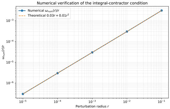
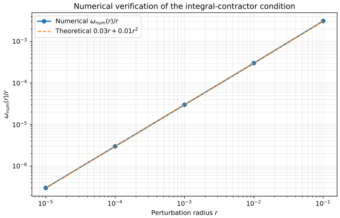
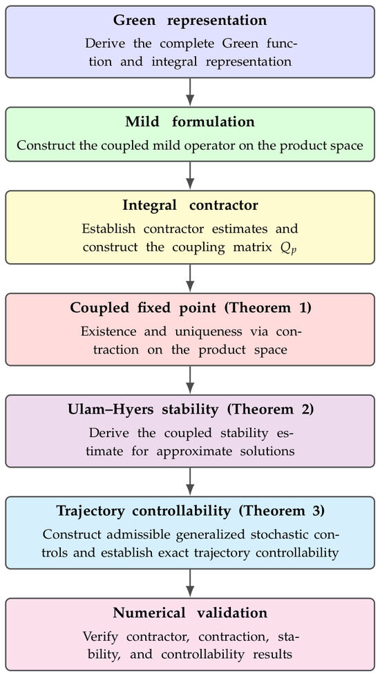
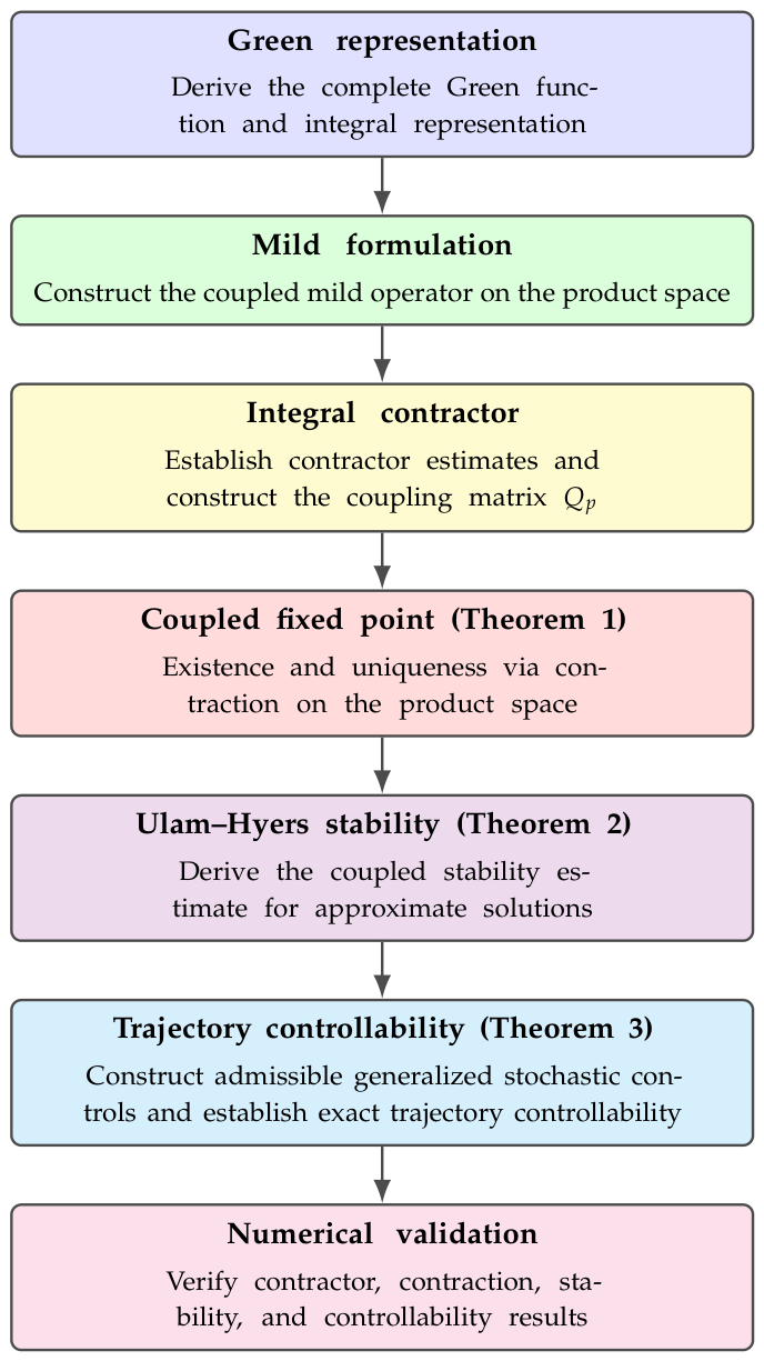
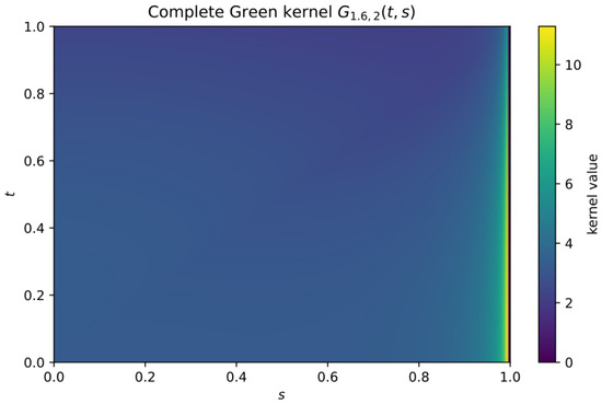
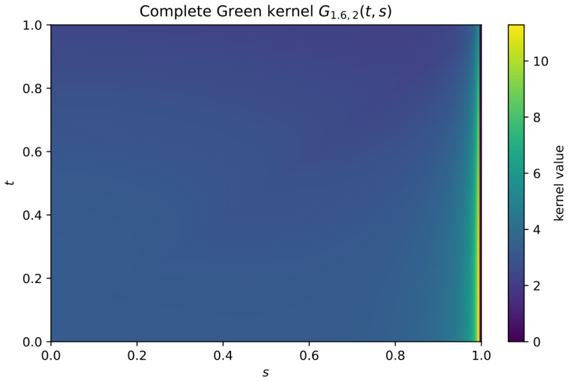
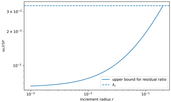
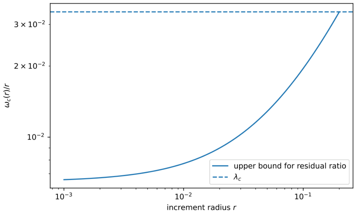
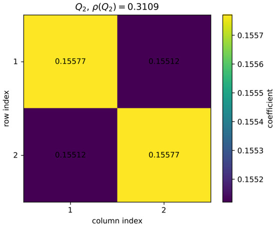
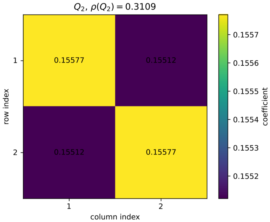
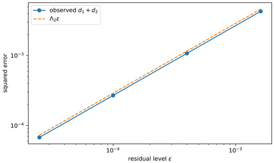
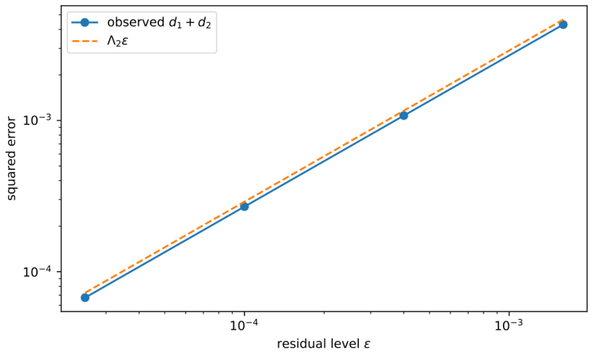
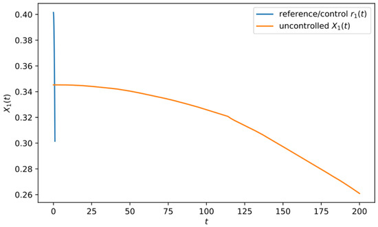
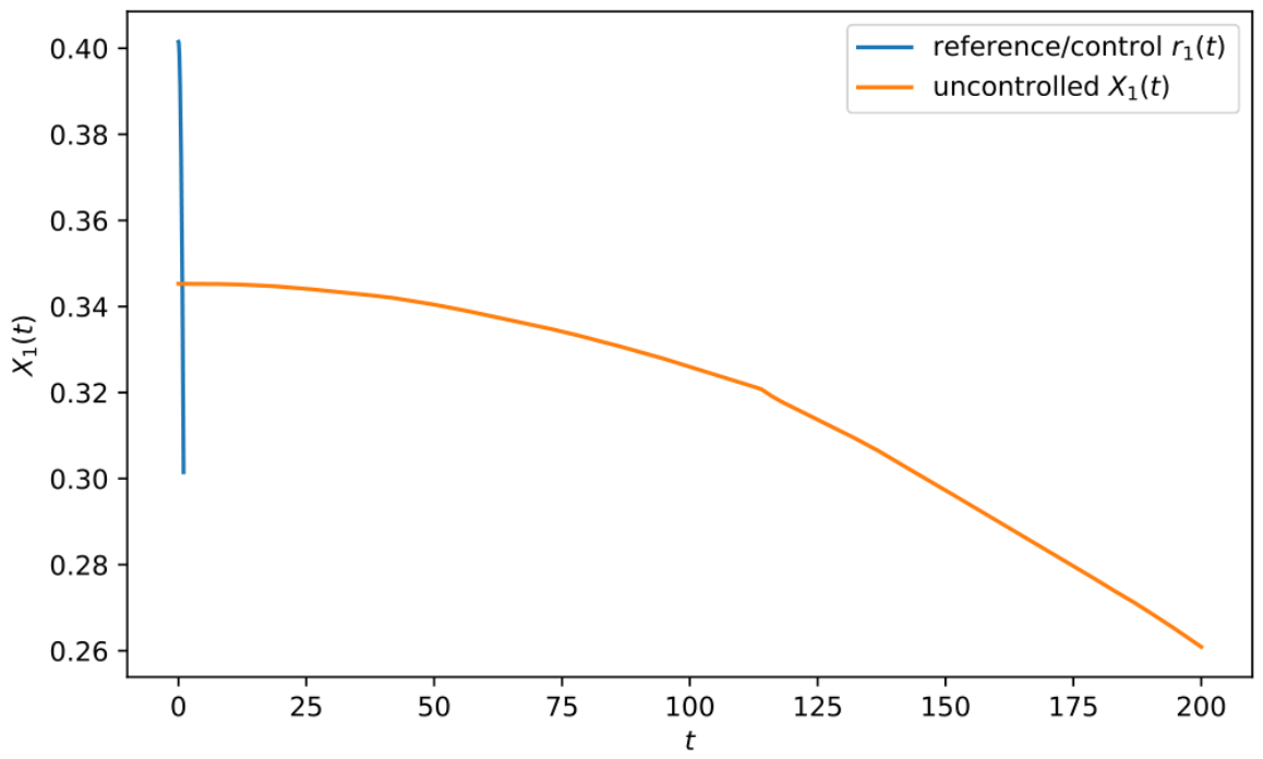

Disclaimer/Publisher’s Note: The statements, opinions and data contained in all publications are solely those of the individual author(s) and contributor(s) and not of MDPI and/or the editor(s). MDPI and/or the editor(s) disclaim responsibility for any injury to people or property resulting from any ideas, methods, instructions or products referred to in the content. |
© 2026 by the authors. Licensee MDPI, Basel, Switzerland. This article is an open access article distributed under the terms and conditions of the Creative Commons Attribution (CC BY) license.