


Abstract
We introduce a combinatorial p-th geodesic curvature flow for ideal circle patterns in spherical background geometry, where . We prove that, for any initial data, the flow has a unique solution for all time. Moreover, prescribed total geodesic curvatures can be realized by a spherical ideal circle pattern if and only if the solution of the flow converges for some initial data, or equivalently, for any initial data. In the realizable case, the solution converges in finite time for , exponentially fast for , and at an algebraic rate for . For a constrained flow preserving the sum of the logarithmic curvatures, we characterize convergence to a uniformly shifted target and show that the preserved sum determines the limiting metric. Finally, we characterize the admissible targets by positive edge allocations and obtain a vertexwise sufficient condition for existence.
Keywords:
combinatorial p-th geodesic curvature flow; ideal circle pattern; spherical background geometry; constrained flow MSC:
52C26; 51M10; 53E99
1. Introduction
1.1. Background
Circle packings and circle patterns are closely related to discrete conformal geometry and to the geometry of polyhedra. The classical results of Koebe, Andreev, and Thurston give existence and rigidity theorems for circle packings; see [1,2,3]. Variational methods for circle patterns were developed by Colin de Verdière and by Bobenko–Springborn [4,5]. We also refer to [6,7,8] for related results.
Motivated by Hamilton’s Ricci flow [9], Chow and Luo [10] introduced the combinatorial Ricci flow for circle packing metrics on triangulated surfaces. Since then, combinatorial Ricci and Calabi flows have been studied in several discrete conformal settings; see, for example, [11,12]. In particular, Lin and Zhang introduced the combinatorial p-th Calabi flow [13] and the combinatorial p-th Ricci flow [14] on triangulated surfaces. Feng, Lin, and Zhang further studied combinatorial p-th Calabi flows for discrete conformal factors [15]. These works provide the basic nonlinear p-flow framework for the flow considered in the present paper. For ideal circle patterns in Euclidean and hyperbolic background geometries, Ge–Hua–Zhou [16] proved that the convergence of the combinatorial Ricci flow is equivalent to the existence of a circle pattern with the prescribed curvature.
In spherical background geometry, prescribing the cone angles does not in general give a rigidity theorem, because of the action of Möbius transformations. Nie [17] showed that existence and rigidity are recovered by prescribing the total geodesic curvature of each circle. His proof is based on a strictly convex variational functional. Using this functional, Ge–Hua–Zhou [18] introduced a combinatorial geodesic curvature flow and characterized its convergence. Further developments concerning spherical Calabi flows and degenerate targets can be found in [19,20,21], and the infinite case is treated in [22]. Related results for generalized hyperbolic circle patterns are contained in [23,24,25,26,27].
The character approach gives local conditions for the existence of circle packings. Ge and Lin introduced the character of Thurston’s circle packings in hyperbolic background geometry and obtained vertexwise criteria for their existence [28]. Li, Lin, and Shen subsequently developed the character of ideal circle patterns and derived criteria which can be checked at individual vertices [29].
In this paper, we consider a combinatorial p-th geodesic curvature flow in spherical background geometry for every . When , it is the flow studied by Ge–Hua–Zhou. We prove that the flow has a unique solution for all time for any initial metric. The prescribed total geodesic curvature is realizable if and only if the solution converges for some initial metric, or equivalently, for every initial metric. In the realizable case, the convergence is in finite time for , exponential for , and algebraic for . The uniqueness argument for uses the sign properties of the Jacobian of the curvature map, since the vector field is not locally Lipschitz at an equilibrium.
We also consider a constrained flow which preserves . Its limiting curvature is in general of the form . Finally, we give a characterization of the admissible data and derive a vertexwise sufficient condition for existence.
1.2. Spherical Ideal Circle Patterns
Let be a finite simple graph giving a closed cell decomposition of a closed surface S, with vertex set V, edge set E, and face set F. Thus G has no loops and no multiple edges, so an unordered pair determines at most one edge; this is the setting of all the statements below. Every vertex is assumed to be incident to an edge. We write for an edge with endpoints and for adjacency. The domain E of the angle assignment is this same edge set. We follow the vertex-indexed convention of Ge–Hua–Zhou; it is dual to Nie’s face-indexed convention.
Write . After fixing an ordering of V, we identify the space of real functions on V with :
The latter set is the open positive orthant of , not a vector subspace. We use bold symbols for vectors, such as and , and subscripts for their scalar components. All vectors are column vectors. The symbols denote vertex indices and e denotes an edge; these are not vector quantities. The matrix J will denote the Jacobian of the curvature map, and will denote a scalar potential.
Choose for each . For , take two spherical disks of radii whose overlap is a bigon of interior angle at each corner. Joining the disk centers to the two corners gives a spherical quadrilateral. Glue these quadrilaterals along their radial sides according to the cell decomposition. The resulting cone surface carries disks with boundary circles ; the construction is the dual form of Proposition 6 of [17].
Here, ideal means that the complement of the open disks consists of the finitely many intersection points corresponding to faces of G: there are no open interstices. It does not refer to points at infinity or to a limiting value of the radii. Cone singularities are allowed at these intersection points and at the vertices corresponding to the disk centers. The non-obtuse range is the class covered by the circle-pattern construction and rigidity theorem used here. It ensures that the overlap bigons have disjoint interiors; zero angles would give degenerate bigons.
Let be the cone angle at the vertex corresponding to in this vertex-indexed decomposition. The length of is
Since the geodesic curvature of is , its total geodesic curvature is
Given , the prescribed total geodesic curvature problem is to find radii such that
For , let
Define
Nie proved the following existence and rigidity theorem (Theorem 1 of [17]).
Theorem 1.
Let . There exists a spherical ideal circle pattern with combinatorial data and total geodesic curvature if and only if . If it exists, the pattern is unique up to isotopy.
To study the prescribed problem by a flow, we use the coordinate
The map is a diffeomorphism from onto , and
1.3. Main Results
With , let . For , let
We consider the system
Theorem 2.
Let and .
- (a)
- (b)
- The following statements are equivalent:
- (c)
- Suppose that the equivalent conditions in (b) hold, and let be the unique vector satisfying . Then, for every initial value,
- (i)
- converges to exponentially if ;
- (ii)
- if ;
- (iii)
- If , there exists such that for all .
We next consider the constrained system
For , set
Theorem 3.
for a unique . If and , then if and only if .
Let and . For every , Equation (7) has a unique solution for all and preserves . Moreover, the following statements are equivalent:
- (i)
- ;
- (ii)
- There are and such that ;
- (iii)
- The solution converges for every initial value in ;
- (iv)
- The solution converges for some initial value in .
- If these conditions hold, the limit is the unique vector in satisfying
For each edge , write . Choose positive numbers and satisfying
For such a choice, put
Theorem 4.
For , the following statements are equivalent:
- (i)
- ;
- (ii)
In particular, the symmetric choice gives the sufficient condition
The edge-weight condition in Theorem 4 is equivalent to Nie’s admissibility inequalities; the allocation argument behind it goes back to Proposition 4 of [5] and Proposition 13 of [17]. Here it is used to pass between the admissibility inequalities and the vertexwise condition (10). The symmetric condition (11) depends only on the edges adjacent to a single vertex; it is sufficient but is not necessary in general.
2. Preliminaries
2.1. The Variational Functional
We first recall the variational properties of the total geodesic curvature. For an edge , let be the length of the arc of in the corresponding bigon and set
Then
For finite , the radii lie in , so both boundary arcs of each bigon have positive length and positive geodesic curvature. Thus . The bigon is a nondegenerate disk without cone points and has area . With its positively oriented boundary, each corner has exterior turning angle . Gauss–Bonnet therefore gives
or equivalently
Since and , this yields . Summing over the nonempty collection of edges incident to i proves
The upper bound depends only on the fixed edge angles. No lower bound for or for is used, so it remains a uniform bound along sequences approaching either endpoint. The strict inequalities are asserted for finite ; at a degenerate limiting configuration, equality may occur.
For each , the one-form
is closed. Let be a primitive of . The Hessian of is positive definite. Moreover,
and the same inequalities hold after interchanging i and j; see Lemma 9 of [17] and Lemma 2.1 of [18].
Set
Then
The matrix is symmetric and positive definite. Its off-diagonal entries are nonpositive, and its row sums are positive:
Indeed, when i and j are joined by an edge and is zero otherwise, while
For , define
It follows that
A continuous function on , or on an affine subspace of , is called proper if each of its sublevel sets is compact. The following facts are due to Nie (Proposition 13 of [17]); they are also recalled in Theorem 3.2 of [18].
Proposition 1.
The function is smooth and strictly convex on , with gradient and positive definite Hessian J. It is proper on if and only if . Its critical points are precisely the vectors satisfying . For admissible , its unique minimum is attained at this vector.
Theorem 1 characterizes geometric realizability. Proposition 1 gives the corresponding variational criterion and supplies the compact sublevel sets used in the convergence proof.
2.2. The Geodesic Curvature Flows
Definition 1.
Let and . The combinatorial p-th geodesic curvature flow with prescribed total geodesic curvature is
whereis defined in (5).
By (4), the equivalent radius form is
In the geodesic-curvature variable , it becomes
When , Equations (25) and (26) reduce to the prescribed geodesic curvature flow considered in [18,21]. In particular, the existence criterion and exponential convergence in this case recover the nondegenerate spherical result of [18]. The degenerate targets allowed in [21] lie outside the nondegenerate radius range considered here.
The p-th Calabi flows in [13,15] use a discrete p-Laplacian acting on curvature differences along edges of a triangulation. For admissible target curvatures, Liu, Li, and Qi [20] prove global existence and convergence of a spherical p-th Calabi flow for total geodesic curvatures. Their evolution contains the discrete p-Laplacian and the curvature-dependent term in Equation (4) of [20]. In (24), instead acts separately on the components of , giving the dissipation . Theorem 2 establishes uniqueness for and the three convergence regimes, while Theorem 3 characterizes the shifted equilibrium selected by the constrained flow.
The constrained flow (7) is
Its equivalent forms in the variables and are
2.3. Spherical Characters
We use the character notation of [29]. For , define
Thus is determined by the weighted edges adjacent to i.
For each edge , choose such that
For this choice of edge weights, write
at each vertex i. For the symmetric choice , it reduces to .
3. Proof of Theorem 2
3.1. Long-Time Existence and Uniqueness
For , the function is not locally Lipschitz at the origin. Thus uniqueness does not follow directly from the usual local existence theorem. The sign of the curvature Jacobian in (20) gives the required comparison principle.
Lemma 1
(Finite maxima and comparison). Let be functions on a time interval and set . Then h is locally Lipschitz, and its upper right Dini derivative satisfies
If a locally Lipschitz function h satisfies and whenever , then throughout the interval.
Proof.
On every compact time interval the derivatives of the finitely many are bounded, so their maximum is Lipschitz. At a fixed time, the indices that do not attain the maximum have a positive gap and cannot maximize for sufficiently small positive increments. For the remaining indices, the expansions are uniform over this finite set. Taking their maximum proves (36).
For the comparison statement, suppose that on a nonempty connected component of its positivity set, and let a be the left endpoint. Continuity and give . On each compact subinterval of this component, h is absolutely continuous and almost everywhere, so h is nonincreasing there. Letting the left endpoint of the subinterval tend to a gives , a contradiction. If throughout the interval, apply the comparison statement to for any initial time a. It follows that whenever , so h is nonincreasing. □
Lemma 2.
Proof.
Let and be two solutions and set . By the mean value formula,
The off-diagonal entries of are nonpositive and all its row sums are positive. If , then
and the second inequality is strict when , because the row sums of are positive. Since is strictly increasing, the flow equation gives at every maximum index, with strict inequality if . Although the vector field need not be locally Lipschitz, its solutions are because the vector field is continuous. Lemma 1 therefore applies to and gives whenever . As , its comparison statement yields . Interchanging and gives . Hence .
For the constrained flow, summing the equations shows . Put
If , then the maximum of is positive and its minimum is negative. By (38), at every maximum index; in the same way, at every minimum index. Hence
at a maximum index, and the reverse inequality holds at a minimum index. If , then the difference of the two flow equations is . Write and . Since is a finite maximum of functions, Lemma 1 gives the explicit formula
whenever . The common term has canceled. The comparison statement of Lemma 1, together with and , now gives . Together with , this yields . □
Lemma 3.
Proof.
The total geodesic curvature is a smooth function of . Since is continuous for , the flow has a local solution for every initial value. Lemma 2 gives its uniqueness.
It remains to prove that the solution cannot escape to infinity in finite time. By (15),
Hence is bounded by a constant depending only on p, , and . The solution stays in a bounded set on every finite time interval and therefore extends to all . □
3.2. Convergence and Convergence Rates
We shall use the following estimate for the prescribed curvature potential.
Lemma 4.
Suppose that and let be determined by . Let be a compact convex set containing , and assume that
for some . Then, for ,
where and the constant used in all rate estimates is
Proof.
Write . Since the Hessian of is J, the lower bound for J gives
On the other hand, the equivalence of the finite-dimensional norms gives
For , this is . For , Hölder’s inequality gives , which yields the stated factor after taking the p-th power. Combining these estimates proves (39). □
Lemma 5.
Proof.
By Proposition 1, the strictly convex potential is proper and has a unique critical point . Along the flow, (27) gives
Thus the trajectory lies in the compact sublevel set
The set Q is convex. Since is positive definite and depends continuously on , there is a constant such that
Set
By Lemma 4 and (27),
In particular, . The same lower bound for J gives
and hence . □
Lemma 6.
Proof.
Since , the potential has a finite limit. Integrating (27) gives
By continuity, the integrand converges to . This limit must be zero, for otherwise (45) would fail. Thus . Theorem 1 now implies . □
Lemma 3 proves Theorem 2(a). Theorem 1, together with Lemmas 5 and 6, proves the equivalence in Theorem 2(b). We next make the rates precise.
Lemma 7.
- (a)
- If , then
- (b)
- If , thenand consequently .
- (c)
- If , then for all , where
The same qualitative rates hold for .
Proof.
If , then and uniqueness in Lemma 2 gives the constant solution. In part (b), the displayed expression is used when ; when , the bound is simply . Suppose . For , (43) gives . If , division by and integration give (47). If and Y remained positive beyond the time in (48), the same calculation would give
a contradiction. Hence for some finite T. Since is strictly convex, . The constant curve solves the same autonomous equation with initial value at . The shifted curve has that initial value as well. Lemma 2 therefore gives for all , including when . No local Lipschitz assumption at the equilibrium is needed.
□
This completes the proof of Theorem 2.
4. Proof of Theorem 3
We first establish global well-posedness, the preserved quantity, and the energy identity for the constrained flow defined in (29).
Proposition 2.
For every and every initial value, the constrained flow (29) has a unique solution for all . Along this solution,
Moreover,
where
The dissipation vanishes if and only if .
Proof.
From the definition of , we have
Thus is nonempty precisely when the left endpoint in (52) is strictly smaller than the right endpoint. In particular, whenever .
Proof of Theorem 3.
The first assertion follows from Proposition 2. We prove the equivalence of (i)–(iv).
Suppose first that . Choose and put . Then . For we have
By Proposition 1, is proper on . It follows from (53) that is proper on . Since its Hessian is positive definite, its restriction to has a unique minimum, denoted by . At this point the derivative of vanishes in every direction tangent to . Therefore, all the numbers are equal, and
for some . Since the left-hand side is the curvature of a spherical ideal circle pattern, Theorem 1 shows that . This proves (i)⇒(ii). The reverse implication follows immediately from Theorem 1.
Let now be a solution with . By (50) and the properness just proved, the whole trajectory is contained in the compact set
Moreover,
The velocity of the solution is bounded, and is uniformly continuous on . Hence (55) implies
Every limit point of therefore satisfies . Thus is a critical point of the restriction of to , and consequently . It follows that the whole solution converges to . We have proved (i)⇒(iii), and (iii)⇒(iv) is clear.
Conversely, suppose that a solution in converges to . Integrating (50) and using the convergence of show that . Hence for some . This proves (iv)⇒(ii).
The strict convexity of on gives the uniqueness of . Equation (54) then gives the uniqueness of . Finally, assume that and let . If , then the invariance of gives . Conversely, if , then is the unique minimum of on , so every solution in this hyperplane converges to . □
We finally describe the dependence of the constant on . For , let be the unique vector realizing . Differentiating gives
Consequently, is the unique multiplier for which . In particular, both and are independent of p; the exponent changes the trajectory and its rate but not the constrained limit.
The constrained flow above is different from the usual normalization in Euclidean background geometry. Indeed, summing the bigon Gauss–Bonnet identity (14) over all edges gives
which varies with . Hence, even when , the term does not vanish in general. In Euclidean background geometry, the constant direction comes from scaling, and the total combinatorial curvature is fixed by the Gauss–Bonnet formula. In spherical background geometry, however, is positive definite. Thus the additional term in (29) imposes a genuine constraint and changes the prescribed-curvature problem.
5. Proof of Theorem 4
We first record the edge-weight lemma needed in the proof. It is the finite-graph form of the allocation argument used in Proposition 4 of [5] and Proposition 13 of [17].
Lemma 8.
Let for and let for . Suppose that
Then there are numbers , one for each end i of an edge e, such that
Proof.
For , set
Every is nonempty because there are no isolated vertices. There are finitely many such sets, so we may take
Then for every edge and
Set and choose a finite number . Form a directed network with source s, sink t, one node for each edge e, and one node for each vertex i. Give capacity , each of and capacity B when , and capacity .
We check every source–sink cut. If a cut crosses an arc of capacity B, its capacity exceeds D. Otherwise, let X be the set of vertex nodes on the sink side. Each edge node incident to X must also be on the sink side since placing it on the source side would cross an arc of capacity B. The cut therefore has capacity at least
For , the first sum already equals D; for nonempty X, the inequality follows from (61). Conversely, the cut immediately before the sink has capacity D. The max-flow min-cut theorem [30] thus gives a flow of value D for this finite network with real capacities.
All arcs are saturated, because their capacities sum to D. Let be the flow on . Conservation at the vertex nodes and edge nodes gives, respectively,
This proves (60). □
Proof of Theorem 4.
We first prove (ii)⇒(i). Suppose that positive numbers satisfying (8) and (10) are given. For any nonempty , we have
To justify the edge count, let consist of edges with both endpoints in X and of edges with exactly one endpoint in X. Then and
Each internal edge contributes exactly , and each boundary edge contributes less than because its other weight is positive. The first inequality above is strict even when is empty, since X is nonempty and the vertex inequalities are strict. Hence .
We next prove (i)⇒(ii). Apply Lemma 8 with and . For , write and . We then have
Define
The unused capacity is positive on every edge. Adding half to each end makes both weights strictly positive and gives . At vertex i,
The final inequality is strict because every vertex is incident to at least one edge with positive unused capacity. This establishes (i)⇒(ii).
The admissibility inequality for a single vertex also gives the following obstruction.
Proposition 3.
If there exists such that
then no spherical ideal circle pattern realizes , and no solution of (24) converges in .
Proof.
For , the admissibility inequality reads
Corollary 1.
Let . If
then there is a unique spherical ideal circle pattern satisfying . It is obtained by the p-th flow for every .
Proof.
The assumption gives for every , so the conclusion follows from Theorem 4. □
Example 1.
The symmetric character condition is sufficient but not necessary. Consider the triangle graph with on each of its three edges. The character is at every vertex. The target
does not satisfy the symmetric character condition at the first vertex. Nevertheless, every singleton inequality is bounded by , every two-vertex inequality by , and the total sum is . Hence . By Theorem 4, there are nonsymmetric edge weights for which at every vertex.
6. Numerical Illustration
On a three-cycle, we compare the distance to equilibrium for and examine the shifted equilibrium of the constrained flow.
6.1. The Numerical Setting
Let G be the three-cycle with and
For , the local total geodesic curvature is computed from
Here is the length of the corresponding circle arc. The convention is . In (66), , and for all finite . Thus the selected angle is the first-quadrant value , including when . This is the half-angle of the sector at vertex i.
We take and set
and use in the three unconstrained computations. The Dormand–Prince explicit Runge–Kutta method of order 8(5,3) (DOP853) is used with relative tolerance and absolute tolerance . The intervals for are , , and , respectively. For , the computation is stopped at the first downward crossing of . The script reproduce_numerics.py (File S1), recorded output (File S2), and execution instructions (File S3) are provided in the Supplementary Materials. The reported run uses Python 3.13.5, NumPy 2.1.3, SciPy 1.15.3, and Matplotlib 3.10.0. For the decay fits, we sample the dense output at 501 equally spaced times on when , and at 501 geometrically spaced times on when . The constrained diagnostics use 1001 equally spaced times on .
A centered finite-difference approximation with step to has symmetry error , minimum eigenvalue , largest off-diagonal entry , and minimum row sum . These values agree with the properties in (20).
6.2. Numerical Results
- The case .
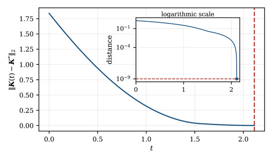
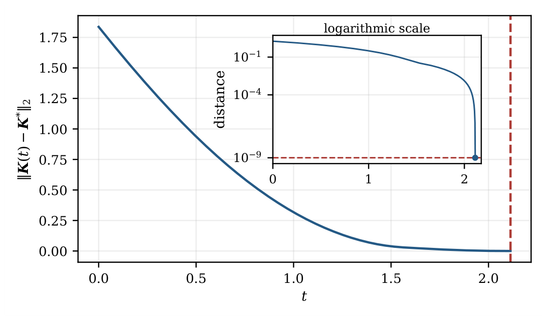
The distance first crosses at ; this time is marked by the vertical dashed line in Figure 1. The inset shows the same trajectory on a logarithmic vertical scale; the dot marks the computed endpoint, and the horizontal dashed line indicates the threshold. The rapid decrease is consistent with the finite-time convergence in Theorem 2(c)(iii). Reaching a fixed numerical tolerance is not, by itself, a proof of exact stabilization.
Figure 1.
Evolution of for . The blue curves show the Euclidean distance between the logarithmic geodesic-curvature vector and its equilibrium . The red vertical dashed line marks the first crossing of . The inset uses a logarithmic vertical scale; its red horizontal dashed line marks this threshold, and the blue dot marks the computed endpoint.
Near , subtraction in is affected by floating-point cancellation. For , a residual perturbation of size produces a velocity of order , and is unbounded at zero. An adaptive explicit solver may therefore take very small steps or show small oscillations about equilibrium instead of returning an exactly constant vector. With the stopping distance fixed at , tightening the integrator tolerances from to and then to gives event times that agree to six decimal places under all three tolerance settings. Repeating the computation with stopping distances and gives event times and , respectively, compared with at ; these values show the dependence on the stopping threshold. The target is evaluated as in full working precision; the rounded values in (67) are for display only.
For , the theoretical estimate (48) reads
Numerical quadrature gives , and denotes the first exact arrival time. Evaluating requires a certified lower bound for the smallest eigenvalue of J on the entire sublevel set (41). The value computed at characterizes the Hessian only at that point.
- The case .
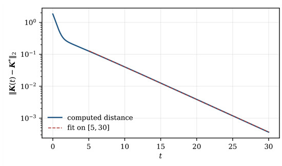
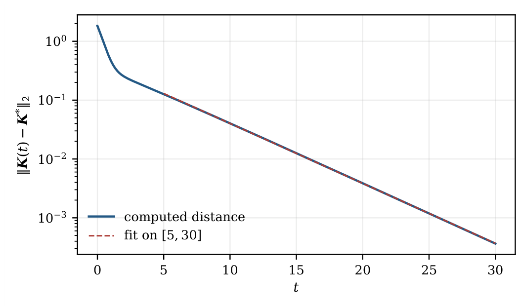
Figure 2 shows the computed distance as a solid curve on a semilogarithmic scale. Regressing on t over the finite window gives slope with coefficient of determination ; the dashed curve shows this fit. The nearly linear profile agrees with the exponential convergence in Theorem 2(c)(i). Moving the left end of the window to 10 or to 15 changes the slope to or to , so the fitted value reflects the window as well as the trajectory.
Figure 2.
Semilogarithmic plot of for .
- The case .
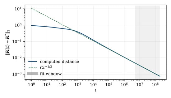
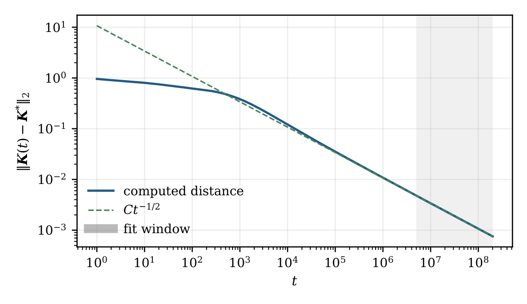
In Figure 3, both axes are logarithmic. The solid curve shows the computed distance, and the dashed reference curve is normalized to this distance at . The shaded region marks the fitting window. Over the finite window , the fitted log–log slope is with , close to , in agreement with the algebraic decay in Theorem 2(c)(ii). Moving the left end of the window to or to changes the slope to or to .
Figure 3.
Log–log plot of for .
- The constrained flow with .
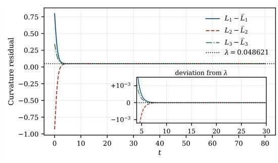
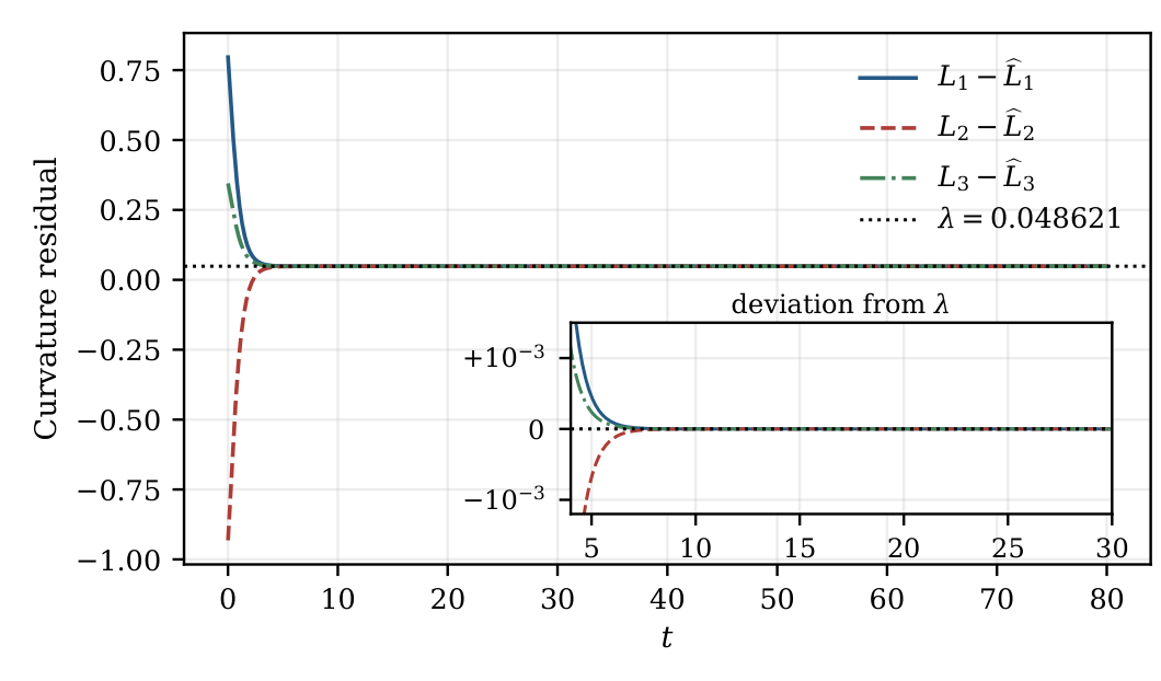
Take , so that while ; the two metrics lie in different invariant hyperplanes. At the 1001 sampled times , , the maximum absolute deviation of from its initial value was approximately , at the level of floating-point round-off. Figure 4 shows that the three residuals converge to the common value , whereas . The horizontal dotted line marks the common shift, and the inset shows the componentwise deviations from it on a scale of . Thus the limit satisfies , rather than , as stated in Theorem 3.
Figure 4.
Curvature residuals for the constrained flow with . The curves show for ; the dotted line marks the common shift . The inset shows deviations from . Coincidence of the curves near the limit reflects convergence to this common value.
The numerical values discussed above are summarized in Table 1.
Table 1.
Summary of the numerical results.
Supplementary Materials
The following supporting information can be downloaded at https://www.mdpi.com/article/10.3390/axioms15100718/s1, File S1: reproduce_numerics.py, numerical reproduction code; File S2: numerical_results.json, recorded numerical output; File S3: README_numerics.txt, execution instructions.
Funding
This research received no external funding.
Institutional Review Board Statement
Not applicable.
Informed Consent Statement
Not applicable.
Data Availability Statement
The original contributions presented in this study are included in the article and its Supplementary Materials. No external datasets were used. The numerical results in Section 6 can be reproduced using File S1; the recorded output is provided in File S2. Further inquiries can be directed to the corresponding author.
Conflicts of Interest
The author declares no conflicts of interest.
References
- Koebe, P. Kontaktprobleme der konformen Abbildung. Ber. Verh. Sächs. Akad. Wiss. Leipz. Math.-Phys. Kl. 1936, 88, 141–164. [Google Scholar]
- Andreev, E.M. On convex polyhedra in Lobachevskii spaces. Math. USSR-Sb. 1970, 10, 413–440. [Google Scholar] [CrossRef] [Scilit]
- Thurston, W.P. The Geometry and Topology of Three-Manifolds; Collected Works; American Mathematical Society: Providence, RI, USA, 2022; Volume 4. [Google Scholar]
- Colin de Verdière, Y. Un principe variationnel pour les empilements de cercles. Invent. Math. 1991, 104, 655–669. [Google Scholar] [CrossRef] [Scilit]
- Bobenko, A.I.; Springborn, B.A. Variational principles for circle patterns and Koebe’s theorem. Trans. Am. Math. Soc. 2004, 356, 659–689. [Google Scholar] [CrossRef] [Scilit]
- Rivin, I. Euclidean structures on simplicial surfaces and hyperbolic volume. Ann. Math. 1994, 139, 553–580. [Google Scholar] [CrossRef] [Scilit] [PubMed][Green Version]
- Stephenson, K. Introduction to Circle Packing: The Theory of Discrete Analytic Functions; Cambridge University Press: Cambridge, UK, 2005. [Google Scholar]
- Rodin, B.; Sullivan, D. The convergence of circle packings to the Riemann mapping. J. Differ. Geom. 1987, 26, 349–360. [Google Scholar] [CrossRef] [Scilit]
- Hamilton, R.S. Three-manifolds with positive Ricci curvature. J. Differ. Geom. 1982, 17, 255–306. [Google Scholar] [CrossRef] [Scilit]
- Chow, B.; Luo, F. Combinatorial Ricci flows on surfaces. J. Differ. Geom. 2003, 63, 97–129. [Google Scholar] [CrossRef] [Scilit]
- Ge, H. Combinatorial Calabi flows on surfaces. Trans. Am. Math. Soc. 2018, 370, 1377–1391. [Google Scholar] [CrossRef] [Scilit]
- Ge, H.; Hua, B. On combinatorial Calabi flow with hyperbolic circle patterns. Adv. Math. 2018, 333, 523–538. [Google Scholar] [CrossRef] [Scilit]
- Lin, A.; Zhang, X. Combinatorial p-th Calabi flows on surfaces. Adv. Math. 2019, 346, 1067–1090. [Google Scholar] [CrossRef] [Scilit]
- Lin, A.; Zhang, X. Combinatorial p-th Ricci flows on surfaces. Nonlinear Anal. 2021, 211, 112417. [Google Scholar] [CrossRef] [Scilit]
- Feng, K.; Lin, A.; Zhang, X. Combinatorial p-th Calabi flows for discrete conformal factors on surfaces. J. Geom. Anal. 2020, 30, 3979–3994. [Google Scholar] [CrossRef] [Scilit]
- Ge, H.; Hua, B.; Zhou, Z. Combinatorial Ricci flows for ideal circle patterns. Adv. Math. 2021, 383, 107698. [Google Scholar] [CrossRef] [Scilit]
- Nie, X. On circle patterns and spherical conical metrics. Proc. Am. Math. Soc. 2024, 152, 843–853. [Google Scholar] [CrossRef] [Scilit]
- Ge, H.; Hua, B.; Zhou, P. A combinatorial curvature flow in spherical background geometry. J. Funct. Anal. 2024, 286, 110335. [Google Scholar] [CrossRef] [Scilit]
- Lei, Z.; Zhou, P. Combinatorial Calabi flows for ideal circle patterns in spherical background geometry. J. Differ. Equ. 2025, 427, 676–688. [Google Scholar] [CrossRef] [Scilit]
- Liu, B.; Li, L.; Qi, Y. Combinatorial p-th Calabi flows for total geodesic curvatures in spherical background geometry. Adv. Nonlinear Anal. 2025, 14, 20250067. [Google Scholar] [CrossRef] [Scilit]
- Hu, G.; Lei, Z.; Sun, Y.; Zhou, P. The convergence of prescribed combinatorial Ricci flows for total geodesic curvatures in spherical background geometry. arXiv 2024, arXiv:2404.05982. [Google Scholar]
- Li, C.; Lu, Y.; Yu, H. Infinite combinatorial Ricci flow in spherical background geometry. arXiv 2025, arXiv:2505.05925. [Google Scholar]
- Ge, H.; Hua, B.; Zhou, Z. Circle patterns on surfaces of finite topological type. Am. J. Math. 2021, 143, 1397–1430. [Google Scholar] [CrossRef] [Scilit]
- Ba, T.; Hu, G.; Sun, Y. Circle packings and hyperbolic surfaces of finite type. Calc. Var. Partial. Differ. Equ. 2025, 64, 262. [Google Scholar] [CrossRef] [Scilit]
- Ba, T.; Zheng, C. Combinatorial curvature flows for generalized hyperbolic circle packings on surfaces. Nonlinear Anal. 2025, 255, 113773. [Google Scholar] [CrossRef] [Scilit]
- Hu, G.; Qi, Y.; Sun, Y.; Zhou, P. Hyperbolic circle packings and total geodesic curvatures on surfaces with boundary. Nonlinear Anal. 2025, 253, 113735. [Google Scholar] [CrossRef] [Scilit]
- Hu, G.; Lei, Z.; Qi, Y.; Zhou, P. Combinatorial p-th Calabi flows for total geodesic curvatures in hyperbolic background geometry. J. Geom. Anal. 2025, 35, 18. [Google Scholar] [CrossRef] [Scilit]
- Ge, H.; Lin, A. The character of Thurston’s circle packings. Sci. China Math. 2024, 67, 1623–1640. [Google Scholar] [CrossRef] [Scilit]
- Li, C.; Lin, A.; Shen, L. The character of ideal circle patterns. arXiv 2026, arXiv:2602.19748. [Google Scholar]
- Ford, L.R., Jr.; Fulkerson, D.R. Maximal flow through a network. Can. J. Math. 1956, 8, 399–404. [Google Scholar] [CrossRef] [Scilit]

Disclaimer/Publisher’s Note: The statements, opinions and data contained in all publications are solely those of the individual author(s) and contributor(s) and not of MDPI and/or the editor(s). MDPI and/or the editor(s) disclaim responsibility for any injury to people or property resulting from any ideas, methods, instructions or products referred to in the content. |
© 2026 by the author. Licensee MDPI, Basel, Switzerland. This article is an open access article distributed under the terms and conditions of the Creative Commons Attribution (CC BY) license.