On the Spectral Analysis of Diamond-α Sturm–Liouville Problems on Uniform Time Scales

Abstract

This paper investigates a Sturm–Liouville problem formulated in terms of the diamond-$\alpha$ derivative on a uniform time scale. The proposed setting combines the delta and nabla components within a unified spectral framework. A key feature of this framework is the explicit identification of the defect structure arising from diamond-$\alpha$ integration by parts, which distinguishes the resulting spectral theory from its classical continuous counterpart. Under appropriate regularity and uniqueness assumptions, a conditional linear-dependence criterion is established for solutions corresponding to the same eigenvalue, whereas eigenfunctions associated with distinct eigenvalues satisfy an orthogonality relation under a suitable compatibility condition. A generalized Green identity is derived, and the resulting remainder term is shown to define a skew-symmetric defect form. Moreover, an explicit estimate for this term is obtained, yielding $R_{\alpha }(u,v)=O\left(\nu \right)$ as the graininess $\nu$ tends to zero under uniform boundedness assumptions. When the boundary form vanishes and the spectral gap remains uniformly separated from zero, this estimate further implies asymptotic orthogonality of eigenfunctions associated with distinct eigenvalues in the dense-limit regime. A generalized integral identity for the eigenfunctions is also established. The classical continuous structure is recovered when $\mathbb{T}=\mathbb{R}$, while the defect term vanishes in the dense-limit regime under the stated boundedness assumptions.

1. Introduction

Time scale calculus, initiated by Hilger in 1988 [1], provides a unified framework for studying differential and difference equations within the same mathematical setting. The delta derivative ($\Delta$) and the nabla derivative (∇) provide two complementary approaches to differentiation on time scales, corresponding to the forward and backward dynamic calculi, respectively [2,3,4,5,6]. Further developments in the fundamental calculus on time scales, including integration theory and applications to various mathematical models, can be found in [7,8,9].

A significant extension of these ideas is the diamond-$\alpha$ derivative introduced by Sheng et al. [10]. The diamond-$\alpha$ operator combines the forward and backward dynamic differentiation mechanisms through the weighting parameter $\alpha$. In particular, $\alpha =1$ recovers the delta derivative ($\Delta$), while the endpoint $\alpha =0$ formally corresponds to the nabla derivative (∇). Throughout the present work, however, we restrict our analysis to $\alpha \in (0,1]$; hence, the nabla endpoint is mentioned only as a formal limiting case. On the continuous time scale $\mathbb{T}=\mathbb{R}$, both notions reduce to the ordinary derivative. Subsequent studies have developed the diamond-$\alpha$ framework in several directions. Rogers and Sheng [11] investigated fundamental properties of the diamond dynamic derivative, while diamond-$\alpha$ dynamic equations and related analytical properties were further studied in [12,13,14]. Integral formulations, mean value results, and polynomial-series representations associated with the diamond-$\alpha$ calculus were developed in [15,16,17]. More recent extensions include combined measure and integration theories [18,19], diamond-$\alpha$ Hardy–Copson and Grüss-type inequalities [20,21,22], as well as stability properties of discrete diamond-$\alpha$ operators [23,24].

Spectral problems on time scales have been investigated from several complementary perspectives. Amster et al. [25] studied detailed eigenvalue asymptotics, while Huseyinov and Bairamov [26] considered eigenfunction expansions for second-order dynamic equations. Guseinov [27] investigated self-adjoint boundary-value problems and symmetric Green’s functions, whereas Rynne [28] developed an $L_2$ framework for boundary-value problems on time scales. Related qualitative results for difference equations, particularly oscillation properties, were obtained in [29].

Sturm–Liouville spectral theory on time scales has been developed in several directions. Agarwal et al. [30] considered Sturm–Liouville eigenvalue problems on time scales, whereas Guseinov [31] studied the corresponding eigenfunction expansions. Spectral problems involving parameter-dependent conditions were investigated for discrete Sturm–Liouville equations in [32], for Sturm–Liouville operators on time scales in [33], and for dissipative Sturm–Liouville operators on bounded time scales in [34]. Related spectral developments include diffusion equations on time scales [35], eigenparameter-dependent quantum difference equations [36], and Dirac systems on time scales [37].

The Sturm–Liouville equation plays a fundamental role in mathematical physics and arises naturally in the spectral analysis of many differential models [38]. This motivates the study of its diamond-$\alpha$ counterpart on uniform time scales. In contrast to formulations based solely on delta or nabla differentiation, the present problem incorporates both operators through the diamond-$\alpha$ derivative. More recently, diamond-type dynamic operators have also been employed in the spectral analysis of Dirac-type systems on time scales [39]. The purpose of this work is therefore to investigate the resulting spectral structure and to determine which fundamental properties of Sturm–Liouville theory are preserved in this combined setting.

An essential feature of the present formulation is that the diamond-$\alpha$ operator does not simply replace one dynamic derivative with another. Instead, it combines the forward and backward differentiation mechanisms through a weighting parameter. As a consequence, some arguments familiar from classical Sturm–Liouville theory cannot be transferred directly to the diamond-$\alpha$ setting. In particular, integration by parts generates additional terms that influence the corresponding Green identity and, consequently, the orthogonality analysis. This makes it necessary to explicitly identify the assumptions under which the fundamental spectral properties remain valid.

Another point of interest is the relation between the combined time scale formulation and the classical continuous problem. A satisfactory extension should preserve the characteristic features of the continuous Sturm–Liouville equation as the underlying time scale becomes dense. For this reason, special attention is devoted to the case $\mathbb{T}=\mathbb{R}$. This reduction provides a useful consistency check for the proposed framework and clarifies the role of the additional terms that arise specifically in the diamond-$\alpha$ setting.

The specific novelty of the present work lies in identifying the structural consequences of combining the delta and nabla dynamics within a Sturm–Liouville spectral framework. In the purely delta or purely nabla formulations, the corresponding one-sided calculus determines the associated integration-by-parts and Green-type structures. In the diamond-$\alpha$ setting considered here, however, the simultaneous presence of the two dynamic directions generates additional shifted contributions that cannot, in general, be reduced to the classical boundary term.

Accordingly, the contribution of this study is not merely to replace a delta or nabla derivative with a weighted diamond-$\alpha$ derivative. The analysis isolates an explicit defect form $R_{\alpha }$, establishes its skew-symmetry and dependence on graininess, and shows how this term modifies the usual Green identity, symmetry, and orthogonality mechanisms. In particular, exact orthogonality is formulated through a combined boundary–defect compatibility condition, while asymptotic orthogonality is obtained under the stated boundedness and uniform spectral-gap assumptions in the dense-limit regime. The special balanced case $\alpha =1/2$ is also shown not to eliminate the defect in general.

Motivated by these observations, the present study focuses on the spectral structure generated by the diamond-$\alpha$ operator on a uniform time scale. Rather than assuming that the classical spectral properties are automatically preserved, we explicitly identify the additional uniqueness and compatibility requirements needed for the analysis.

• Comparison with Existing Literature. Classical spectral problems on time scales have been studied mainly within delta- or nabla-based frameworks, including self-adjoint boundary-value problems and Sturm–Liouville eigenvalue problems [27,28,30,31,33,34]. The diamond-$\alpha$ derivative, introduced as a weighted combination of the delta and nabla derivatives in [10], provides a different structure by simultaneously incorporating forward and backward dynamic components. Diamond-type operators have also been considered more recently in the spectral analysis of Dirac systems on time scales [39]. In contrast to the one-sided Sturm–Liouville formulations described above, the present framework shows that the interaction between the delta and nabla components generates additional shift-dependent terms in the integration-by-parts structure, giving rise to the defect form $R_{\alpha }$. Consequently, the Green identity, symmetry mechanism, and orthogonality relation involve additional compatibility requirements. The present study focuses specifically on these structural effects and their dependence on the graininess parameter, including the dense-limit estimate $R_{\alpha }=O\left(\nu \right)$ under the stated boundedness assumptions.

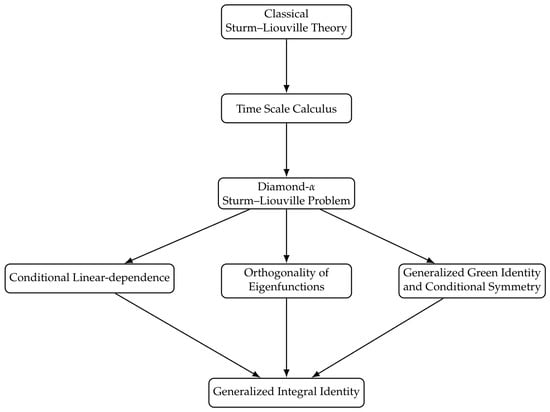
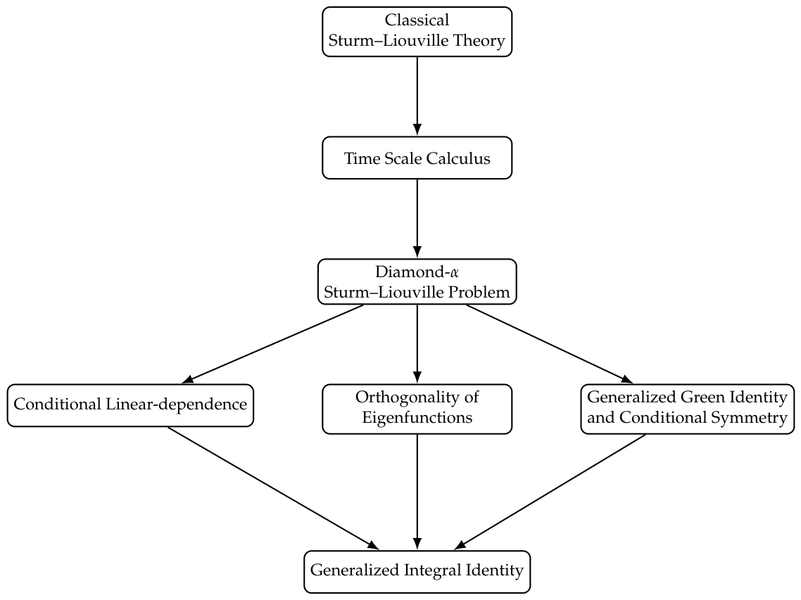
• Contributions of this Paper. The main novelty of the present work lies not merely in replacing the classical derivative with the diamond-$\alpha$ operator, but also in identifying the additional defect structure generated by the interaction of the delta and nabla components and determining its consequences for Green-type identities, symmetry, and orthogonality. The following is a summary of the paper’s key contributions (as shown in Figure 1):
  

  Figure 1. Schematic overview of the proposed diamond-$\alpha$ Sturm–Liouville framework and its main theoretical results. Source: Authors’ own elaboration.
  • A diamond-$\alpha$ Sturm–Liouville problem is formulated on a uniform time scale.
  • A conditional linear-dependence criterion is established for solutions associated with the same eigenvalue, while orthogonality of eigenfunctions corresponding to distinct eigenvalues is obtained under an appropriate compatibility condition.
  • A generalized Green identity is derived, and the associated remainder term is characterized as a skew-symmetric defect form. Furthermore, an explicit estimate for this term is established, showing that

    $$R_{\alpha }(u,v)=O\left(\nu \right)$$

    in the dense-limit regime, provided the relevant norms remain uniformly bounded. When the boundary form vanishes and the spectral gap remains uniformly separated from zero, this estimate also yields asymptotic orthogonality of eigenfunctions corresponding to distinct eigenvalues.
  • A generalized integral identity associated with the eigenfunctions is derived, incorporating the additional remainder term generated by diamond-$\alpha$ integration by parts.

2. Preliminaries on Diamond-$\mathit{\alpha }$ Calculus

This section recalls the basic concepts of diamond-$\alpha$ calculus required for the subsequent spectral analysis. Throughout this paper, $\mathbb{T}$ denotes a uniform time scale, and the standard notation of time scale calculus is adopted. Only those definitions and properties that are directly used in the formulation and analysis of the diamond-$\alpha$ Sturm–Liouville problem are included.

Definition 1

([2]). For a time scale $\mathbb{T}$ and $t\in \mathbb{T}$, set

$$\sigma \left(t\right)=inf\{s\in \mathbb{T}:s>t\},\rho \left(t\right)=sup\{s\in \mathbb{T}:s<t\}.$$

These mappings describe the forward and backward jumps, respectively. As usual, ${\mathbb{T}}^{\kappa }$ denotes $\mathbb{T}$ with a left-scattered maximum removed, if such a point exists, whereas ${\mathbb{T}}_{\kappa }$ is obtained by removing a right-scattered minimum, if such a point exists.

For completeness, we recall the delta and nabla derivatives [2]. A function $h:\mathbb{T}\to \mathbb{R}$ is delta differentiable at $t\in {\mathbb{T}}^{\kappa }$ if there exists a number $h^{\Delta }\left(t\right)$ such that, for every $\epsilon >0$, there exists a neighborhood U of t satisfying

$$\left|h\left(\sigma \left(t\right)\right)-h\left(s\right)-h^{\Delta }\left(t\right)(\sigma \left(t\right)-s)\right|\le \epsilon |\sigma \left(t\right)-s|,s\in U.$$

Similarly, h is nabla differentiable at $t\in {\mathbb{T}}_{\kappa }$ if there exists a number $h^{\nabla }\left(t\right)$ such that, for every $\epsilon >0$, there exists a neighborhood V of t satisfying

$$\left|h\left(\rho \left(t\right)\right)-h\left(s\right)-h^{\nabla }\left(t\right)(\rho \left(t\right)-s)\right|\le \epsilon |\rho \left(t\right)-s|,s\in V.$$

Here, $h^{\Delta }\left(t\right)$ and $h^{\nabla }\left(t\right)$ denote the delta derivative and the nabla derivative of h at t, respectively.

Theorem 1

([10]). Let $\alpha \in (0,1]$. If h admits both delta and nabla derivatives on ${\mathbb{T}}_{\kappa }^{\kappa }$, then its diamond-α derivative exists and satisfies

$$h^{{\diamond }_{\alpha }}\left(s\right)=\alpha h^{\Delta }\left(s\right)+(1-\alpha )h^{\nabla }\left(s\right),s\in {\mathbb{T}}_{\kappa }^{\kappa }.$$

Here, ${\mu }_t=\sigma \left(t\right)-t$ and ${\nu }_t=t-\rho \left(t\right)$ denote the forward and backward graininess functions, respectively [2].

Lemma 1

([11]). Every diamond-α differentiable function is continuous at each point at which its diamond-α derivative exists.

We also use the standard regressivity notation of time scale calculus [2]. Thus,

$$\mathcal{R}=\{p:1+{\mu }_{t,t}p\left(t\right)\ne 0\},{\mathcal{R}}_{\nu }=\{p:1-{\nu }_{t,t}p\left(t\right)\ne 0\},$$

on their corresponding time scale domains.

Lemma 2

([10]). Let $h_1,h_2:\mathbb{T}\to \mathbb{R}$ be ${\diamond }_{\alpha }$ differentiable. The ${\diamond }_{\alpha }$ derivative is linear, and its product rule is given by

$${\left(h_1{h}_2\right)}^{{\diamond }_{\alpha }}=h_1^{{\diamond }_{\alpha }}{h}_2+\alpha h_1^{\sigma }{h}_2^{\Delta }+(1-\alpha )h_1^{\rho }{h}_2^{\nabla }.$$

Here, $h_1^{\rho }\left(t\right)=h_1\left(\rho \left(t\right)\right)$ and $h_1^{\sigma }\left(t\right)=h_1\left(\sigma \left(t\right)\right)$ denote the backward and forward shifts of $h_1$, respectively [2].

Lemma 3

([10]). Let $\alpha \in (0,1]$ and let $h:\mathbb{T}\to \mathbb{R}$ be integrable in both the delta and nabla senses. The ${\diamond }_{\alpha }$ integral of h over ${[a,b]}_{\mathbb{T}}$ is given by the following weighted combination

$${\int }_a^{b}h\left(l\right){\diamond }_{\alpha }l=\alpha {\int }_a^{b}h\left(l\right)\Delta l+(1-\alpha ){\int }_a^{b}h\left(l\right)\nabla l.$$

Definition 2.

Let $y_1$ and $y_2$ be ${\diamond }_{\alpha }$ differentiable functions on $\mathbb{T}$. The diamond-α Wronskian associated with $y_1$ and $y_2$ is defined by

$$W_{{\diamond }_{\alpha }}(y_1,y_2):=y_1{y}_2^{{\diamond }_{\alpha }}-y_2{y}_1^{{\diamond }_{\alpha }}.$$

For any function f defined on $\mathbb{T}$, we use the standard shift notation

$$f^{\sigma }\left(t\right):=f\left(\sigma \left(t\right)\right),f^{\rho }\left(t\right):=f\left(\rho \left(t\right)\right).$$

Accordingly,

$$W_{{\diamond }_{\alpha }}^{\sigma }(u,v)\left(t\right):=W_{{\diamond }_{\alpha }}(u,v)\left(\sigma \left(t\right)\right),W_{{\diamond }_{\alpha }}^{\rho }(u,v)\left(t\right):=W_{{\diamond }_{\alpha }}(u,v)\left(\rho \left(t\right)\right).$$

The same convention applies to shifted derivatives; for example,

$${\left(u^{{\diamond }_{\alpha }}\right)}^{\sigma }\left(t\right)=u^{{\diamond }_{\alpha }}\left(\sigma \left(t\right)\right),{\left(u^{{\diamond }_{\alpha }}\right)}^{\rho }\left(t\right)=u^{{\diamond }_{\alpha }}\left(\rho \left(t\right)\right).$$

3. Spectral Analysis of Diamond-$\mathit{\alpha }$ Sturm–Liouville Problems

In this section, we formulate the ${\diamond }_{\alpha }$ Sturm–Liouville problem on a uniform time scale and investigate its principal spectral properties. In particular, we establish a conditional linear-dependence criterion and an orthogonality result, derive a Green-type identity, and obtain a generalized integral identity associated with the eigenfunctions. Consider

$$\begin{array}{ccc}\hfill L_{{\diamond }_{\alpha }}y=-y^{{\diamond }_{\alpha }{\diamond }_{\alpha }}\left(t\right)+p\left(t\right)y\left(t\right)& =& \lambda y\left(t\right),t\in {\mathbb{T}}^{*},\hfill \end{array}$$

(1)

$$\begin{array}{ccc}\hfill y^{{\diamond }_{\alpha }}\left(t_0\right)& =& y_0,\hfill \end{array}$$

(2)

$$\begin{array}{ccc}\hfill \alpha \beta y^{{\diamond }_{\alpha }}\left(\rho \left(t_0\right)\right)& =& \alpha \beta y_0,\hfill \end{array}$$

(3)

where $\beta =1-\alpha$, ${\mathbb{T}}^{*}=\mathbb{T}\setminus \{min\mathbb{T},max\mathbb{T}\}$, $t_0\in {\mathbb{T}}^{*}$, $y_0\in \mathbb{R}$, $p\in \mathcal{R}\cap {\mathcal{R}}_{\nu }$, and $\alpha \in (0,1]$.

Throughout Section 3, unless otherwise stated, we assume that $\mathbb{T}$ is a regular uniform time scale, that $\alpha \in (0,1]$, and that

$$p\in \mathcal{R}\cap {\mathcal{R}}_{\nu }.$$

We further assume that all functions under consideration possess the delta, nabla, and diamond-$\alpha$ derivatives required for the corresponding results and that all products and expressions appearing in the relevant diamond-$\alpha$ integrals are integrable on the intervals considered. Any additional regularity, uniqueness, boundedness, or compatibility assumptions required for a particular result are stated explicitly therein.

For clarity, we specify the operator-theoretic framework adopted throughout the paper. Let

$$L_{{\diamond }_{\alpha }}y=-y^{{\diamond }_{\alpha }{\diamond }_{\alpha }}+p\left(t\right)y$$

be defined on the associated real weighted space

$$L_{{\diamond }_{\alpha }}^2[a,b],{⟨u,v⟩}_{{\diamond }_{\alpha }}={\int }_a^{b}u\left(t\right)v\left(t\right){\diamond }_{\alpha }t.$$

The admissible domain is defined by

$${\mathcal{D}}_{max}\left(L_{{\diamond }_{\alpha }}\right)=\left\{y\in L_{{\diamond }_{\alpha }}^2[a,b]:y,y^{{\diamond }_{\alpha }},y^{{\diamond }_{\alpha }{\diamond }_{\alpha }}\mathrm{exist},\mathrm{and}{L}_{{\diamond }_{\alpha }}y\in L_{{\diamond }_{\alpha }}^2[a,b]\right\}.$$

(4)

The prescribed conditions (2) and (3) are not incorporated into the linear operator domain in (4). Instead, they define the admissible solution class

$${\mathcal{A}}_{y_0}=\left\{y\in {\mathcal{D}}_{max}\left(L_{{\diamond }_{\alpha }}\right):y^{{\diamond }_{\alpha }}\left(t_0\right)=y_0,\alpha \beta y^{{\diamond }_{\alpha }}\left(\rho \left(t_0\right)\right)=\alpha \beta y_0\right\}.$$

When $y_0\ne 0$, the set ${\mathcal{A}}_{y_0}$ need not be a linear space and is therefore not treated as the domain of a linear operator. The differential expression

$$L_{{\diamond }_{\alpha }}y=-y^{{\diamond }_{\alpha }{\diamond }_{\alpha }}+p\left(t\right)y$$

is considered on the linear maximal domain ${\mathcal{D}}_{max}\left(L_{{\diamond }_{\alpha }}\right)$, whereas the prescribed conditions (2) and (3) are imposed separately on solutions of the specific problem (1)–(3).

It should be emphasized that conditions (2) and (3) are prescribed conditions of the present diamond-$\alpha$ formulation and do not, in general, constitute a pair of classical separated Sturm–Liouville boundary conditions. Accordingly, within the prescribed-data formulation considered in this paper, we define a real parameter $\lambda$ as an admissible spectral value whenever there exists a nonzero function

$$y\in {\mathcal{A}}_{y_0}$$

satisfying

$$L_{{\diamond }_{\alpha }}y=\lambda y.$$

The corresponding function y is referred to as an admissible eigenfunction in the terminology of the present work. This terminology is used only within the stated regularity, existence, uniqueness, and compatibility assumptions and should not be interpreted as asserting that (1)–(3) define a classical linear self-adjoint Sturm–Liouville eigenvalue problem. For brevity, in the subsequent statements the terms “eigenvalue” and “eigenfunction” refer to an admissible spectral value and its corresponding admissible eigenfunction, respectively, in the sense specified above.

• Spectral existence assumption. Throughout the spectral analysis below, we assume that the admissible problem (1)–(3) possesses at least one nontrivial solution for at least one real value of the spectral parameter $\lambda$. More generally, whenever eigenfunctions corresponding to one or more eigenvalues are considered, the existence of the corresponding eigenpairs $(\lambda ,y)$ is assumed.

The purpose of the present work is not to establish a general existence theory for the spectrum of the diamond-$\alpha$ problem, but rather to investigate the structural properties of admissible eigenpairs when they exist. In particular, the results concerning linear dependence, orthogonality, the generalized Green identity, and asymptotic orthogonality are conditional upon the existence of the eigenpairs involved. Establishing sufficient conditions for the existence, discreteness, and completeness of the spectrum requires a separate operator-theoretic analysis and is left for future investigation.

The conditions (2) and (3) are regarded as prescribed data associated with the present diamond-$\alpha$ formulation. Since they do not, in general, constitute a standard pair of separated Sturm–Liouville boundary conditions, the spectral statements established below are understood only under the uniqueness and compatibility assumptions explicitly stated in the corresponding results. In particular, uniqueness of the corresponding initial-value problem is imposed as an additional hypothesis whenever it is required and is not inferred from (2) and (3).

Lemma 4

([39]). Let $h:\mathbb{T}\to \mathbb{R}$ be ${\diamond }_{\alpha }$ integrable for every ξ in ${\mathbb{T}}_{\kappa }^{\kappa }$ and $\alpha \in (0,1],a,b\in {\mathbb{T}}^{*}.$ Then the following identity holds:

$${\displaystyle \underset{a}{\overset{b}{\int }}}{h}^{{\diamond }_{\alpha }}\left(\xi \right){\diamond }_{\alpha }\xi ={\kappa }_{\alpha }h\left(\xi \right){\mid }_a^b+\alpha \beta \left(h\left(\rho \right(\xi \left)\right)+h\left(\sigma \right(\xi )\right){\mid }_a^b,$$

where ${\kappa }_{\alpha }={\alpha }^2+{\beta }^2$.

Lemma 5

([39]). Let $a,b\in {\mathbb{T}}^{*}$ and let $h_1,h_2:\mathbb{T}\to \mathbb{R}$ be both delta and nabla differentiable, with all terms appearing below diamond-α integrable on $[a,b]$. Let $\alpha \in (0,1]$. Then the following diamond-α integration-by-parts formula holds:

$$\begin{array}{ccc}\hfill {\displaystyle \underset{a}{\overset{b}{\int }}}{h}_1^{{\diamond }_{\alpha }}\left(\xi \right)h_2\left(\xi \right){\diamond }_{\alpha }\xi & =& {\kappa }_{\alpha }\left(h_1{h}_2\right)\left(\xi \right){\mid }_a^b+\alpha \beta \left[{\left(h_1{h}_2\right)}^{\rho }\left(\xi \right)+{\left(h_1{h}_2\right)}^{\sigma }\left(\xi \right)\right]{\mid }_a^b\hfill \\ & & +\beta {\displaystyle \underset{a}{\overset{b}{\int }}}{h}_2^{\nabla }\left(\xi \right)\left[h_1^{\sigma }\left(\xi \right)-h_1^{\rho }\left(\xi \right)\right]{\diamond }_{\alpha }\xi -{\displaystyle \underset{a}{\overset{b}{\int }}}{h}_1^{\sigma }\left(\xi \right)h_2^{{\diamond }_{\alpha }\left(\xi \right)}{\diamond }_{\alpha }\xi .\hfill \end{array}$$

This identity will be used as the integration-by-parts formula for the diamond-$\alpha$ operator in the subsequent spectral arguments.

We now investigate the spectral properties of the operator $L_{{\diamond }_{\alpha }}$ within the framework of the problem (1)–(3). We first establish a conditional linear-dependence criterion for solutions corresponding to the same eigenvalue. For this purpose, we assume that the associated diamond-$\alpha$ initial-value problem is uniquely solvable at each admissible initial point $t_i\in {\mathbb{T}}^{*}$ with initial data of the form

$$y\left(t_i\right)=c_0,y^{{\diamond }_{\alpha }}\left(t_i\right)=c_1.$$

This uniqueness property is imposed as an additional hypothesis and is not derived from conditions (2) and (3).

Theorem 2.

Let $y_1$ and $y_2$ be two solutions corresponding to the same eigenvalue λ. Assume that the uniqueness property stated above holds. If 

$$W_{{\diamond }_{\alpha }}(y_1,y_2)\left(t_i\right)=0,$$

then $y_1$ and $y_2$ are linearly dependent.

Proof. 

By Definition 2,

$$W_{{\diamond }_{\alpha }}(y_1,y_2)\left(t_i\right)=y_1\left(t_i\right)y_2^{{\diamond }_{\alpha }}\left(t_i\right)-y_2\left(t_i\right)y_1^{{\diamond }_{\alpha }}\left(t_i\right).$$

Hence, the assumption

$$W_{{\diamond }_{\alpha }}(y_1,y_2)\left(t_i\right)=0$$

is equivalent to

$$det\left(\begin{array}{cc}{y}_1\left(t_i\right)& y_2\left(t_i\right)\\ y_1^{{\diamond }_{\alpha }}\left(t_i\right)& y_2^{{\diamond }_{\alpha }}\left(t_i\right)\end{array}\right)=0.$$

Therefore, the vectors

$$\left(y_1\left(t_i\right),y_1^{{\diamond }_{\alpha }}\left(t_i\right)\right)\mathrm{and}\left(y_2\left(t_i\right),y_2^{{\diamond }_{\alpha }}\left(t_i\right)\right)$$

are linearly dependent. Consequently, there exist constants $c_1,c_2\in \mathbb{R}$, not both equal to zero, such that

$$c_1{y}_1\left(t_i\right)+c_2{y}_2\left(t_i\right)=0,$$

and

$$c_1{y}_1^{{\diamond }_{\alpha }}\left(t_i\right)+c_2{y}_2^{{\diamond }_{\alpha }}\left(t_i\right)=0.$$

Set

$$z=c_1{y}_1+c_2{y}_2.$$

Since $y_1$ and $y_2$ correspond to the same eigenvalue and $L_{{\diamond }_{\alpha }}$ is linear,

$$L_{{\diamond }_{\alpha }}z=\lambda z.$$

Moreover,

$$z\left(t_i\right)=z^{{\diamond }_{\alpha }}\left(t_i\right)=0.$$

By the assumed uniqueness of the associated diamond-$\alpha$ initial-value problem, it follows that $z\equiv 0$. Hence,

$$c_1{y}_1+c_2{y}_2=0,$$

and therefore $y_1$ and $y_2$ are linearly dependent.    □

Remark 1.

Theorem 2 provides a conditional linear-dependence criterion. More precisely, under the stated uniqueness assumption, if two solutions $y_1$ and $y_2$ correspond to the same eigenvalue and satisfy

$$W_{{\diamond }_{\alpha }}(y_1,y_2)\left(t_i\right)=0,$$

then $y_1$ and $y_2$ are linearly dependent. Thus, no unconditional linear-dependence statement is asserted; the conclusion holds precisely under the hypotheses stated in Theorem 2.

We next examine eigenfunctions associated with distinct eigenvalues.

To formulate their orthogonality relation, we first introduce the diamond-$\alpha$ inner product and the associated boundary form.

The diamond-$\alpha$ inner product on $L_{{\diamond }_{\alpha }}^2[a,b]$ is defined by

$${⟨u,v⟩}_{{\diamond }_{\alpha }}={\int }_a^{b}u\left(t\right)v\left(t\right){\diamond }_{\alpha }t.$$

By Lemma 3,

$${⟨u,u⟩}_{{\diamond }_{\alpha }}=\alpha {\int }_a^b{\left|u\left(t\right)\right|}^2\Delta t+(1-\alpha ){\int }_a^b{\left|u\left(t\right)\right|}^2\nabla t\ge 0.$$

Hence, the diamond-$\alpha$ pairing is positive semidefinite. After the usual identification of functions that agree almost everywhere with respect to the corresponding weighted measure, it defines the norm

$${\parallel u\parallel }_{{\diamond }_{\alpha }}={\left({\int }_a^b{\left|u\left(t\right)\right|}^2{\diamond }_{\alpha }t\right)}^{1/2}.$$

Accordingly, $L_{{\diamond }_{\alpha }}^2[a,b]$ is understood as the associated weighted $L^2$ space, on which the Cauchy–Schwarz inequality holds with respect to the induced inner product.

To express the Lagrange identity in integral form, we introduce the boundary form arising from the diamond-$\alpha$ integration-by-parts formula in Lemma 5.

For sufficiently regular functions u and v, define the diamond-$\alpha$ boundary form by

$$\begin{array}{cc}\hfill {\mathcal{B}}_{{\diamond }_{\alpha }}(u,v){|}_a^b& :={\kappa }_{\alpha }{W}_{{\diamond }_{\alpha }}(u,\overline{v}){|}_a^b+\alpha \beta \left[W_{{\diamond }_{\alpha }}{(u,\overline{v})}^{\rho }+W_{{\diamond }_{\alpha }}{(u,\overline{v})}^{\sigma }\right]{|}_a^b.\hfill \end{array}$$

The prescribed conditions (2) and (3) should be distinguished from the endpoint conditions appearing in the boundary form above. In particular, conditions (2) and (3), which are imposed at the prescribed point $t_0$ and its backward shift, do not in general imply

$$B_{{\diamond }_{\alpha }}(u,v){|}_a^b=0.$$

Therefore, the vanishing of the boundary form is not assumed to follow automatically from (2) and (3).

More generally, the exact orthogonality result requires the combined condition

$$B_{{\diamond }_{\alpha }}(u,v){|}_a^b+R_{\alpha }(u,v)=0.$$

Thus, the prescribed data (2) and (3) and the endpoint compatibility conditions associated with the generalized Green identity play distinct roles in the present formulation.

Theorem 3

(Generalized Green Identity). Let u and v be sufficiently regular functions on a regular uniform time scale $\mathbb{T}$. Then

$${⟨L_{{\diamond }_{\alpha }}u,v⟩}_{{\diamond }_{\alpha }}-{⟨u,L_{{\diamond }_{\alpha }}v⟩}_{{\diamond }_{\alpha }}=B_{{\diamond }_{\alpha }}(u,v){|}_a^b+{\mathcal{R}}_{\alpha }(u,v),$$

where

$$\begin{array}{cc}\hfill B_{{\diamond }_{\alpha }}(u,v){|}_a^b=& {\kappa }_{\alpha }{W}_{{\diamond }_{\alpha }}(u,v){|}_a^b+\alpha \beta \left[W_{{\diamond }_{\alpha }}^{\rho }(u,v)+W_{{\diamond }_{\alpha }}^{\sigma }(u,v)\right]{|}_a^b,\hfill \end{array}$$

and

$$\begin{array}{cc}\hfill {\mathcal{R}}_{\alpha }(u,v)=& \beta {\int }_a^b\left\{u^{\nabla }\left[{\left(v^{{\diamond }_{\alpha }}\right)}^{\sigma }-{\left(v^{{\diamond }_{\alpha }}\right)}^{\rho }\right]-v^{\nabla }\left[{\left(u^{{\diamond }_{\alpha }}\right)}^{\sigma }-{\left(u^{{\diamond }_{\alpha }}\right)}^{\rho }\right]\right\}{\diamond }_{\alpha }t\hfill \\ & +{\int }_a^b\left[{\left(u^{{\diamond }_{\alpha }}\right)}^{\sigma }{v}^{{\diamond }_{\alpha }}-{\left(v^{{\diamond }_{\alpha }}\right)}^{\sigma }{u}^{{\diamond }_{\alpha }}\right]{\diamond }_{\alpha }t.\hfill \end{array}$$

Proof. 

Since

$$L_{{\diamond }_{\alpha }}u=-u^{{\diamond }_{\alpha }{\diamond }_{\alpha }}+p\left(t\right)u$$

and

$$L_{{\diamond }_{\alpha }}v=-v^{{\diamond }_{\alpha }{\diamond }_{\alpha }}+p\left(t\right)v,$$

we have

$$\begin{array}{cc}& {⟨L_{{\diamond }_{\alpha }}u,v⟩}_{{\diamond }_{\alpha }}-{⟨u,L_{{\diamond }_{\alpha }}v⟩}_{{\diamond }_{\alpha }}\hfill \\ & ={\int }_a^b\left[u{v}^{{\diamond }_{\alpha }{\diamond }_{\alpha }}-v{u}^{{\diamond }_{\alpha }{\diamond }_{\alpha }}\right]{\diamond }_{\alpha }t.\hfill \end{array}$$

Applying Lemma 5 to

$${\int }_a^b{v}^{{\diamond }_{\alpha }{\diamond }_{\alpha }}\left(t\right)u\left(t\right){\diamond }_{\alpha }t,$$

with

$$h_1=v^{{\diamond }_{\alpha }},h_2=u,$$

gives

$$\begin{array}{cc}\hfill {\int }_a^b{v}^{{\diamond }_{\alpha }{\diamond }_{\alpha }}u{\diamond }_{\alpha }t=& {\kappa }_{\alpha }u{v}^{{\diamond }_{\alpha }}{|}_a^b+\alpha \beta \left[{\left(u{v}^{{\diamond }_{\alpha }}\right)}^{\rho }+{\left(u{v}^{{\diamond }_{\alpha }}\right)}^{\sigma }\right]{|}_a^b\hfill \\ & +\beta {\int }_a^b{u}^{\nabla }\left[{\left(v^{{\diamond }_{\alpha }}\right)}^{\sigma }-{\left(v^{{\diamond }_{\alpha }}\right)}^{\rho }\right]{\diamond }_{\alpha }t\hfill \\ & -{\int }_a^b{\left(v^{{\diamond }_{\alpha }}\right)}^{\sigma }{u}^{{\diamond }_{\alpha }}{\diamond }_{\alpha }t.\hfill \end{array}$$

Similarly, applying Lemma 5 with

$$h_1=u^{{\diamond }_{\alpha }},h_2=v,$$

yields

$$\begin{array}{cc}\hfill {\int }_a^b{u}^{{\diamond }_{\alpha }{\diamond }_{\alpha }}v{\diamond }_{\alpha }t=& {\kappa }_{\alpha }v{u}^{{\diamond }_{\alpha }}{|}_a^b+\alpha \beta \left[{\left(v{u}^{{\diamond }_{\alpha }}\right)}^{\rho }+{\left(v{u}^{{\diamond }_{\alpha }}\right)}^{\sigma }\right]{|}_a^b\hfill \\ & +\beta {\int }_a^b{v}^{\nabla }\left[{\left(u^{{\diamond }_{\alpha }}\right)}^{\sigma }-{\left(u^{{\diamond }_{\alpha }}\right)}^{\rho }\right]{\diamond }_{\alpha }t-{\int }_a^b{\left(u^{{\diamond }_{\alpha }}\right)}^{\sigma }{v}^{{\diamond }_{\alpha }}{\diamond }_{\alpha }t.\hfill \end{array}$$

Here the shifted terms arise directly from the diamond-$\alpha$ integration-by-parts formula in Lemma 5. More precisely, the terms ${\left(v^{{\diamond }_{\alpha }}\right)}^{\sigma }$ and ${\left(v^{{\diamond }_{\alpha }}\right)}^{\rho }$ result from applying that formula with $h_1=v^{{\diamond }_{\alpha }}$ and $h_2=u$, whereas ${\left(u^{{\diamond }_{\alpha }}\right)}^{\sigma }$ and ${\left(u^{{\diamond }_{\alpha }}\right)}^{\rho }$ arise from the corresponding application with $h_1=u^{{\diamond }_{\alpha }}$ and $h_2=v$. The boundary contributions obtained from the two applications are combined using

$$W_{{\diamond }_{\alpha }}(u,v)=u{v}^{{\diamond }_{\alpha }}-v{u}^{{\diamond }_{\alpha }}.$$

In particular,

$$u{v}^{{\diamond }_{\alpha }}-v{u}^{{\diamond }_{\alpha }}=W_{{\diamond }_{\alpha }}(u,v),$$

and the same relation applied after the $\rho$- and $\sigma$-shifts produces

$$W_{{\diamond }_{\alpha }}^{\rho }(u,v)\mathrm{and}{W}_{{\diamond }_{\alpha }}^{\sigma }(u,v),$$

respectively. The remaining integral terms do not cancel and are collected into the defect form $R_{\alpha }(u,v)$.

Therefore, subtracting the two integration-by-parts identities and collecting separately the boundary and integral contributions gives

$$\begin{array}{cc}& {⟨L_{{\diamond }_{\alpha }}u,v⟩}_{{\diamond }_{\alpha }}-{⟨u,L_{{\diamond }_{\alpha }}v⟩}_{{\diamond }_{\alpha }}\hfill \\ & ={\kappa }_{\alpha }{W}_{{\diamond }_{\alpha }}(u,v){|}_a^b+\alpha \beta \left[W_{{\diamond }_{\alpha }}^{\rho }(u,v)+W_{{\diamond }_{\alpha }}^{\sigma }(u,v)\right]{|}_a^b+R_{\alpha }(u,v).\hfill \end{array}$$

By the definition of the boundary form, this is precisely

$${⟨L_{{\diamond }_{\alpha }}u,v⟩}_{{\diamond }_{\alpha }}-{⟨u,L_{{\diamond }_{\alpha }}v⟩}_{{\diamond }_{\alpha }}=B_{{\diamond }_{\alpha }}(u,v){|}_a^b+R_{\alpha }(u,v).$$

This completes the proof.    □

Proposition 1.

Let u and v be sufficiently regular functions on a regular uniform time scale $\mathbb{T}$. Then the remainder form appearing in the generalized Green identity satisfies

$$R_{\alpha }(v,u)=-R_{\alpha }(u,v).$$

In particular,

$$R_{\alpha }(u,u)=0.$$

Proof. 

By definition,

$$\begin{array}{cc}\hfill R_{\alpha }(u,v)=& \beta {\int }_a^b\{u^{\nabla }\left[{\left(v^{{\diamond }_{\alpha }}\right)}^{\sigma }-{\left(v^{{\diamond }_{\alpha }}\right)}^{\rho }\right]\hfill \\ & -v^{\nabla }\left[{\left(u^{{\diamond }_{\alpha }}\right)}^{\sigma }-{\left(u^{{\diamond }_{\alpha }}\right)}^{\rho }\right]\}{\diamond }_{\alpha }t\hfill \\ & +{\int }_a^b\left[{\left(u^{{\diamond }_{\alpha }}\right)}^{\sigma }{v}^{{\diamond }_{\alpha }}-{\left(v^{{\diamond }_{\alpha }}\right)}^{\sigma }{u}^{{\diamond }_{\alpha }}\right]{\diamond }_{\alpha }t.\hfill \end{array}$$

Interchanging u and v reverses the sign of each integrand. Consequently,

$$R_{\alpha }(v,u)=-R_{\alpha }(u,v).$$

Taking $v=u$ gives immediately

$$R_{\alpha }(u,u)=0.$$

   □

Remark 2.

The preceding proposition shows that $R_{\alpha }$ is a skew-symmetric bilinear defect term. Hence, the additional contribution generated by diamond-α integration by parts does not affect the diagonal energy relation, since $R_{\alpha }(u,u)=0$, but it may influence mixed pairings of distinct functions. Therefore, $R_{\alpha }$ measures the departure of the diamond-α operator from the classical symmetric Green structure at the level of mixed inner products.

• Interpretation of the defect form. From the viewpoint of the Green identity, the defect form therefore measures the departure of the mixed diamond-$\alpha$ structure from the classical situation in which the difference

  $${⟨L_{{\diamond }_{\alpha }}u,v⟩}_{{\diamond }_{\alpha }}-{⟨u,L_{{\diamond }_{\alpha }}v⟩}_{{\diamond }_{\alpha }}$$

  is determined solely by endpoint terms. Its skew-symmetry is consistent with this interpretation. Moreover, on a uniform time scale the estimate $R_{\alpha }(u,v)=O\left(\nu \right)$, under the assumptions of Proposition 2, shows that this additional forward–backward interaction becomes small in the dense-limit regime.

Proposition 2.

Let $\mathbb{T}$ be a regular uniform time scale with constant graininess ν, and let u and v be sufficiently regular functions such that all the terms below belong to $L_{{\diamond }_{\alpha }}^2[a,b]$. Then

$$\begin{array}{cc}\hfill |R_{\alpha }(u,v)|\le \nu \{& \beta \parallel u^{\nabla }{\parallel }_{{\diamond }_{\alpha }}\left(\parallel {\left(v^{{\diamond }_{\alpha }}\right)}^{\Delta }{\parallel }_{{\diamond }_{\alpha }}+{\parallel {\left(v^{{\diamond }_{\alpha }}\right)}^{\nabla }\parallel }_{{\diamond }_{\alpha }}\right)\hfill \\ & +\beta \parallel v^{\nabla }{\parallel }_{{\diamond }_{\alpha }}\left(\parallel {\left(u^{{\diamond }_{\alpha }}\right)}^{\Delta }{\parallel }_{{\diamond }_{\alpha }}+{\parallel {\left(u^{{\diamond }_{\alpha }}\right)}^{\nabla }\parallel }_{{\diamond }_{\alpha }}\right)\hfill \\ & +\parallel {\left(u^{{\diamond }_{\alpha }}\right)}^{\Delta }{\parallel }_{{\diamond }_{\alpha }}{\parallel v^{{\diamond }_{\alpha }}\parallel }_{{\diamond }_{\alpha }}\hfill \\ & +\parallel {\left(v^{{\diamond }_{\alpha }}\right)}^{\Delta }{\parallel }_{{\diamond }_{\alpha }}{\parallel u^{{\diamond }_{\alpha }}\parallel }_{{\diamond }_{\alpha }}\},\hfill \end{array}$$

at all points where the corresponding delta and nabla shifts and derivatives are defined.

Proof. 

On a regular uniform time scale with constant graininess $\nu$, we have

$$g^{\sigma }-g^{\rho }=\nu (g^{\Delta }+g^{\nabla })$$

and

$$g^{\sigma }-g=\nu g^{\Delta }.$$

Therefore,

$$\begin{array}{cc}& {\left(u^{{\diamond }_{\alpha }}\right)}^{\sigma }{v}^{{\diamond }_{\alpha }}-{\left(v^{{\diamond }_{\alpha }}\right)}^{\sigma }{u}^{{\diamond }_{\alpha }}\hfill \\ & =\left[{\left(u^{{\diamond }_{\alpha }}\right)}^{\sigma }-u^{{\diamond }_{\alpha }}\right]v^{{\diamond }_{\alpha }}-\left[{\left(v^{{\diamond }_{\alpha }}\right)}^{\sigma }-v^{{\diamond }_{\alpha }}\right]u^{{\diamond }_{\alpha }}\hfill \\ & =\nu \left[{\left(u^{{\diamond }_{\alpha }}\right)}^{\Delta }{v}^{{\diamond }_{\alpha }}-{\left(v^{{\diamond }_{\alpha }}\right)}^{\Delta }{u}^{{\diamond }_{\alpha }}\right].\hfill \end{array}$$

Hence, the remainder term can be written as

$$\begin{array}{cc}\hfill R_{\alpha }(u,v)=& \beta \nu {\int }_a^b\{u^{\nabla }\left[{\left(v^{{\diamond }_{\alpha }}\right)}^{\Delta }+{\left(v^{{\diamond }_{\alpha }}\right)}^{\nabla }\right]\hfill \\ & -v^{\nabla }\left[{\left(u^{{\diamond }_{\alpha }}\right)}^{\Delta }+{\left(u^{{\diamond }_{\alpha }}\right)}^{\nabla }\right]\}{\diamond }_{\alpha }t\hfill \\ & +\nu {\int }_a^b\left[{\left(u^{{\diamond }_{\alpha }}\right)}^{\Delta }{v}^{{\diamond }_{\alpha }}-{\left(v^{{\diamond }_{\alpha }}\right)}^{\Delta }{u}^{{\diamond }_{\alpha }}\right]{\diamond }_{\alpha }t.\hfill \end{array}$$

Applying the triangle inequality and the Cauchy–Schwarz inequality with respect to the diamond-$\alpha$ inner product gives the stated estimate.    □

Corollary 1.

Consider a family of regular uniform time scales whose constant graininess satisfies $\nu \to 0$. Assume that the norms on the right-hand side of Proposition 2 remain uniformly bounded. Then

$$R_{\alpha }(u,v)=O\left(\nu \right),\nu \to 0.$$

More precisely, there exists a constant $C>0$, independent of ν for all sufficiently small ν, such that

$$|R_{\alpha }(u,v)|\le C\nu .$$

The constant C may depend on the fixed parameter α, the interval $[a,b]$, and the uniform bounds assumed for the functions and derivatives appearing in Proposition 2, but it does not depend on the graininess ν.

Consequently,

$$R_{\alpha }(u,v)⟶0$$

as the uniform time scale approaches the dense limit.

Proof. 

The conclusion follows directly from Proposition 2, since its right-hand side is proportional to $\nu$ and all remaining norm terms are uniformly bounded.    □

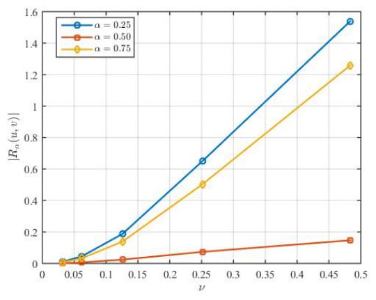
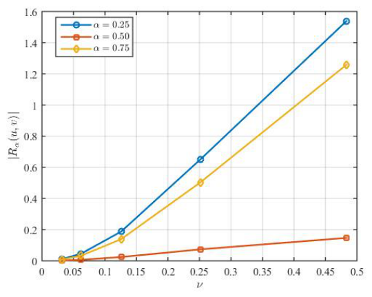
To illustrate the dense-limit behavior stated in Corollary 1, the defect term $R_{\alpha }(u,v)$ was evaluated numerically on the interval $[0,2\pi ]$ using a sequence of uniform time scales. The representative smooth functions were chosen as

$$u\left(t\right)=e^{0.1t}sint,v\left(t\right)=cos\left(2t\right)+0.2sin\left(0.5t\right),$$

with $\alpha =0.25,0.50,$ and $0.75$. The target graininess values were

$$\nu =0.50,0.25,0.125,0.0625,0.03125.$$

For each target value, the number of subintervals was chosen as

$$N=round\left({\displaystyle \frac{2\pi }{\nu }}\right),$$

and the actual uniform graininess used in the computation was $\nu =2\pi /N$.

The delta and nabla derivatives were approximated by the forward and backward difference quotients, respectively, and the diamond-$\alpha$ derivative was then computed from

$$f^{{\diamond }_{\alpha }}=\alpha f^{\Delta }+(1-\alpha )f^{\nabla }.$$

The defect term was evaluated directly from its definition in Theorem 3. The corresponding diamond-$\alpha$ integral was computed as the weighted combination of the discrete delta and nabla sums according to Lemma 3. The resulting values of $|R_{\alpha }(u,v)|$ are displayed on logarithmic axes in Figure 2.

Figure 2. Numerical decay of the diamond-$\alpha$ defect term $|R_{\alpha }(u,v)|$ as the actual uniform graininess $\nu$ decreases on $[0,2\pi ]$, for $u\left(t\right)=e^{0.1t}sint$, $v\left(t\right)=cos\left(2t\right)+0.2sin\left(0.5t\right)$, and $\alpha =0.25,0.50,$ and $0.75$. Both axes are shown on logarithmic scales.

As the graininess decreases, the magnitude of the defect term tends to zero for all considered values of $\alpha$. This numerical behavior is consistent with the dense-limit estimate established in Corollary 1.

In contrast to the classical Sturm–Liouville setting, the diamond-$\alpha$ integration-by-parts formula produces an additional remainder term. Therefore, the vanishing of the boundary form alone is not sufficient in general to ensure orthogonality. This motivates the compatibility condition used in the following theorem.

Theorem 4

(Conditional orthogonality). Let ${\varphi }_1$ and ${\varphi }_2$ be eigenfunctions corresponding to distinct eigenvalues ${\lambda }_1$ and ${\lambda }_2$ of the diamond-α Sturm–Liouville problem. Assume that

$$B_{{\diamond }_{\alpha }}({\varphi }_1,{\varphi }_2){|}_a^b+{\mathcal{R}}_{\alpha }({\varphi }_1,{\varphi }_2)=0.$$

Then ${\varphi }_1$ and ${\varphi }_2$ are orthogonal with respect to the diamond-α inner product, that is,

$${⟨{\varphi }_1,{\varphi }_2⟩}_{{\diamond }_{\alpha }}=0.$$

Proof. 

Since

$$L_{{\diamond }_{\alpha }}{\varphi }_1={\lambda }_1{\varphi }_1,L_{{\diamond }_{\alpha }}{\varphi }_2={\lambda }_2{\varphi }_2,$$

the generalized Green identity gives

$${⟨L_{{\diamond }_{\alpha }}{\varphi }_1,{\varphi }_2⟩}_{{\diamond }_{\alpha }}-{⟨{\varphi }_1,L_{{\diamond }_{\alpha }}{\varphi }_2⟩}_{{\diamond }_{\alpha }}=B_{{\diamond }_{\alpha }}({\varphi }_1,{\varphi }_2){|}_a^b+{\mathcal{R}}_{\alpha }({\varphi }_1,{\varphi }_2).$$

Therefore,

$$({\lambda }_1-{\lambda }_2){⟨{\varphi }_1,{\varphi }_2⟩}_{{\diamond }_{\alpha }}=B_{{\diamond }_{\alpha }}({\varphi }_1,{\varphi }_2){|}_a^b+{\mathcal{R}}_{\alpha }({\varphi }_1,{\varphi }_2).$$

By assumption,

$$B_{{\diamond }_{\alpha }}({\varphi }_1,{\varphi }_2){|}_a^b+{\mathcal{R}}_{\alpha }({\varphi }_1,{\varphi }_2)=0.$$

Since ${\lambda }_1\ne {\lambda }_2$, it follows that

$${⟨{\varphi }_1,{\varphi }_2⟩}_{{\diamond }_{\alpha }}=0.$$

Hence, ${\varphi }_1$ and ${\varphi }_2$ are orthogonal.    □

It is important to emphasize that the preceding orthogonality result is conditional. In contrast to the classical self-adjoint Sturm–Liouville setting, the vanishing of the boundary form alone does not generally imply orthogonality in the present diamond-$\alpha$ framework. The additional defect term $R_{\alpha }({\varphi }_1,{\varphi }_2)$ generated by diamond-$\alpha$ integration by parts must also be taken into account. Thus, exact orthogonality holds only when the combined compatibility condition

$$B_{{\diamond }_{\alpha }}({\varphi }_1,{\varphi }_2){|}_a^b+R_{\alpha }({\varphi }_1,{\varphi }_2)=0$$

is satisfied.

Corollary 2.

Let ${\varphi }_1$ and ${\varphi }_2$ be eigenfunctions corresponding to distinct eigenvalues ${\lambda }_1$ and ${\lambda }_2$. If 

$$B_{{\diamond }_{\alpha }}({\varphi }_1,{\varphi }_2){|}_a^b=0$$

and

$$R_{\alpha }({\varphi }_1,{\varphi }_2)=0,$$

then

$${⟨{\varphi }_1,{\varphi }_2⟩}_{{\diamond }_{\alpha }}=0.$$

Proof. 

Under the stated assumptions,

$$B_{{\diamond }_{\alpha }}({\varphi }_1,{\varphi }_2){|}_a^b+R_{\alpha }({\varphi }_1,{\varphi }_2)=0.$$

Hence, the compatibility condition of Theorem 4 is satisfied, and the conclusion follows directly from that theorem.    □

Proposition 3

(Asymptotic orthogonality). Let $\left\{{\mathbb{T}}_{\nu }\right\}$ be a family of regular uniform time scales with constant graininess $\nu \to 0$. For each ν, let ${\varphi }_{1,\nu }$ and ${\varphi }_{2,\nu }$ be eigenfunctions corresponding to distinct eigenvalues ${\lambda }_{1,\nu }$ and ${\lambda }_{2,\nu }$, respectively. Assume that

$$B_{{\diamond }_{\alpha }}({\varphi }_{1,\nu },{\varphi }_{2,\nu }){|}_a^b=0.$$

Then

$$\left|{⟨{\varphi }_{1,\nu },{\varphi }_{2,\nu }⟩}_{{\diamond }_{\alpha }}\right|={\displaystyle \frac{|R_{\alpha }({\varphi }_{1,\nu },{\varphi }_{2,\nu })|}{|{\lambda }_{1,\nu }-{\lambda }_{2,\nu }|}}.$$

If, in addition, the norms appearing in Proposition 2 remain uniformly bounded with respect to ν and there exists a constant $\delta >0$, independent of ν, such that

$$|{\lambda }_{1,\nu }-{\lambda }_{2,\nu }| \ge \delta$$

for all sufficiently small ν, then

$${⟨{\varphi }_{1,\nu },{\varphi }_{2,\nu }⟩}_{{\diamond }_{\alpha }}=O\left(\nu \right),\nu \to 0.$$

Thus, the corresponding eigenfunction families are asymptotically orthogonal in the dense-limit regime.

Proof. 

Applying the generalized Green identity to ${\varphi }_{1,\nu }$ and ${\varphi }_{2,\nu }$ gives

$$({\lambda }_{1,\nu }-{\lambda }_{2,\nu }){⟨{\varphi }_{1,\nu },{\varphi }_{2,\nu }⟩}_{{\diamond }_{\alpha }}=B_{{\diamond }_{\alpha }}({\varphi }_{1,\nu },{\varphi }_{2,\nu }){|}_a^b+R_{\alpha }({\varphi }_{1,\nu },{\varphi }_{2,\nu }).$$

Since the boundary form vanishes,

$$({\lambda }_{1,\nu }-{\lambda }_{2,\nu }){⟨{\varphi }_{1,\nu },{\varphi }_{2,\nu }⟩}_{{\diamond }_{\alpha }}=R_{\alpha }({\varphi }_{1,\nu },{\varphi }_{2,\nu }).$$

As ${\lambda }_{1,\nu }\ne {\lambda }_{2,\nu }$, it follows that

$$\left|{⟨{\varphi }_{1,\nu },{\varphi }_{2,\nu }⟩}_{{\diamond }_{\alpha }}\right|={\displaystyle \frac{|R_{\alpha }({\varphi }_{1,\nu },{\varphi }_{2,\nu })|}{|{\lambda }_{1,\nu }-{\lambda }_{2,\nu }|}}.$$

By Proposition 2, under the stated uniform boundedness assumptions,

$$R_{\alpha }({\varphi }_{1,\nu },{\varphi }_{2,\nu })=O\left(\nu \right).$$

If the spectral gap is uniformly bounded away from zero, the desired estimate

$${⟨{\varphi }_{1,\nu },{\varphi }_{2,\nu }⟩}_{{\diamond }_{\alpha }}=O\left(\nu \right)$$

follows.    □

The implied constant in this $O\left(\nu \right)$ estimate is independent of $\nu$, but may depend on the fixed parameter $\alpha$, the uniform norm bounds in Proposition 2, and the reciprocal spectral-gap bound ${\delta }^{-1}$. Here the subscripts $\nu$ emphasize that both the eigenvalues and the eigenfunctions may vary with the underlying uniform time scale. The uniform spectral-gap assumption is not asserted to hold automatically; it is an additional hypothesis required to prevent the denominator $|{\lambda }_{1,\nu }-{\lambda }_{2,\nu }|$ from approaching zero as $\nu \to 0$. Without this assumption, the estimate $R_{\alpha }=O\left(\nu \right)$ alone does not imply asymptotic orthogonality.

Remark 3.

The preceding result provides a quantitative counterpart of the classical orthogonality property. Exact orthogonality requires the compatibility condition in Theorem 4. However, when the boundary form vanishes, the defect from orthogonality is controlled by $R_{\alpha }$ and is therefore of order $O\left(\nu \right)$ under the assumptions of Proposition 2 and a uniform spectral-gap condition. In the dense limit, this defect disappears and the classical orthogonality structure is recovered.

Corollary 3.

If

$${\mathcal{R}}_{\alpha }(u,v)=0,$$

then

$${⟨L_{{\diamond }_{\alpha }}u,v⟩}_{{\diamond }_{\alpha }}-{⟨u,L_{{\diamond }_{\alpha }}v⟩}_{{\diamond }_{\alpha }}=B_{{\diamond }_{\alpha }}(u,v){|}_a^b.$$

In particular, if 

$$R_{\alpha }(u,v)=0\mathrm{and}{B}_{{\diamond }_{\alpha }}(u,v){|}_a^b=0$$

for all $u,v$ in a linear realization

$${\mathcal{D}}_{\mathrm{sym}}\subseteq {\mathcal{D}}_{max}\left(L_{{\diamond }_{\alpha }}\right),$$

then $L_{{\diamond }_{\alpha }}$ is symmetric on ${\mathcal{D}}_{\mathrm{sym}}$ with respect to the diamond-α inner product.

• Formal symmetry, symmetry, and self-adjointness. The generalized Green identity allows us to distinguish the relevant operator-theoretic notions in the present setting. Formally, the differential expression

  $${\ell }_{{\diamond }_{\alpha }}\left[y\right]=-y^{{\diamond }_{\alpha }{\diamond }_{\alpha }}+p\left(t\right)y$$

has the classical Sturm–Liouville form. However, in the diamond-$\alpha$ setting, integration by parts yields

$${⟨L_{{\diamond }_{\alpha }}u,v⟩}_{{\diamond }_{\alpha }}-{⟨u,L_{{\diamond }_{\alpha }}v⟩}_{{\diamond }_{\alpha }}=B_{{\diamond }_{\alpha }}(u,v){|}_a^b+R_{\alpha }(u,v).$$

Consequently, formal symmetry in the sense of the differential expression alone does not imply symmetry of the associated operator.

The operator $L_{{\diamond }_{\alpha }}$ is symmetric on a linear realization

$${\mathcal{D}}_{\mathrm{sym}}\subseteq {\mathcal{D}}_{max}\left(L_{{\diamond }_{\alpha }}\right)$$

provided that

$$B_{{\diamond }_{\alpha }}(u,v){|}_a^b+R_{\alpha }(u,v)=0$$

for every $u,v\in {\mathcal{D}}_{\mathrm{sym}}$. A sufficient, but stronger, condition is

$$B_{{\diamond }_{\alpha }}(u,v){|}_a^b=0,R_{\alpha }(u,v)=0,$$

for all $u,v\in {\mathcal{D}}_{\mathrm{sym}}$.

Self-adjointness is a stronger property and would additionally require a specific densely defined linear realization together with the domain equality

$$\mathcal{D}\left(L_{{\diamond }_{\alpha }}\right)=\mathcal{D}\left(L_{{\diamond }_{\alpha }}^{*}\right).$$

Such a realization is not developed in the present work. Therefore, no general self-adjointness claim is made here. Establishing self-adjoint realizations requires a separate analysis of homogeneous boundary conditions and the corresponding operator domains.

Remark 4.

Throughout the present analysis, the spectral problem is considered in the real-valued setting. Accordingly, both eigenvalues and eigenfunctions are taken to be real, and the orthogonality result of Theorem 4 is interpreted within this framework.

We next recall the diamond-$\alpha$ trigonometric identities required for the generalized integral identity.

Lemma 6

([16]). Let $t,t_0\in \mathbb{T}$, $k\left(t\right)=k$ and $1-{\nu }^2{k}^2\ne 0.$ Then,

$$\begin{array}{ccc}\hfill {sin}_k^{{\diamond }_{\alpha }}(t,t_0)& =& {\displaystyle \frac{k}{1+{\nu }^2{k}^2}}\left(\left(1+\alpha {\nu }^2{k}^2\left){cos}_k\right(t,t_0\right)+\beta \nu k{sin}_k(t,t_0)\right),\hfill \\ \hfill {cos}_k^{{\diamond }_{\alpha }}(t,t_0)& =& -{\displaystyle \frac{k}{1+{\nu }^2{k}^2}}\left(\left(1+\alpha {\nu }^2{k}^2\left){sin}_k\right(t,t_0\right)-\beta \nu k{cos}_k(t,t_0)\right),\hfill \end{array}$$

for all $t\in {\mathbb{T}}_{\kappa }^{\kappa },{\nu }_{t,t}=\nu .$

We now derive a generalized integral identity associated with the eigenfunctions of the diamond-$\alpha$ Sturm–Liouville problem. The resulting formula incorporates the boundary, potential, and spectral contributions together with the additional remainder term arising from diamond-$\alpha$ integration by parts.

Lemma 7.

Let $\mathbb{T}$ be a regular uniform time scale and let ν denote its constant graininess. Let $k\in \mathbb{R}$ be constant. For fixed $t\in \mathbb{T}$, the following identities hold with respect to the second variable ω:

$$\begin{array}{cc}\hfill {\left({sin}_k(t,\omega )\right)}_{\omega }^{{\diamond }_{\alpha }}=& -{\displaystyle \frac{k}{1+{\nu }^2{k}^2}}\left[\left(1+\beta {\nu }^2{k}^2\right){cos}_k(t,\omega )+\alpha \nu k{sin}_k(t,\omega )\right],\hfill \\ \hfill {\left({cos}_k(t,\omega )\right)}_{\omega }^{{\diamond }_{\alpha }}=& {\displaystyle \frac{k}{1+{\nu }^2{k}^2}}\left[\left(1+\beta {\nu }^2{k}^2\right){sin}_k(t,\omega )-\alpha \nu k{cos}_k(t,\omega )\right].\hfill \end{array}$$

Proof. 

For fixed t, the delta and nabla derivatives with respect to the second variable $\omega$ satisfy

$$\begin{array}{cc}\hfill {\left({sin}_k(t,\omega )\right)}_{\omega }^{\Delta }& =-{\displaystyle \frac{k}{1+{\nu }^2{k}^2}}\left[{cos}_k(t,\omega )+\nu k{sin}_k(t,\omega )\right],\hfill \\ \hfill {\left({sin}_k(t,\omega )\right)}_{\omega }^{\nabla }& =-k{cos}_k(t,\omega ),\hfill \end{array}$$

and

$$\begin{array}{cc}\hfill {\left({cos}_k(t,\omega )\right)}_{\omega }^{\Delta }& ={\displaystyle \frac{k}{1+{\nu }^2{k}^2}}\left[{sin}_k(t,\omega )-\nu k{cos}_k(t,\omega )\right],\hfill \\ \hfill {\left({cos}_k(t,\omega )\right)}_{\omega }^{\nabla }& =k{sin}_k(t,\omega ).\hfill \end{array}$$

Using

$$f^{{\diamond }_{\alpha }}=\alpha f^{\Delta }+(1-\alpha )f^{\nabla },$$

we obtain

$$\begin{array}{cc}\hfill {\left({sin}_k(t,\omega )\right)}_{\omega }^{{\diamond }_{\alpha }}=& -{\displaystyle \frac{k}{1+{\nu }^2{k}^2}}\left[\left(1+\beta {\nu }^2{k}^2\right){cos}_k(t,\omega )+\alpha \nu k{sin}_k(t,\omega )\right],\hfill \end{array}$$

and

$$\begin{array}{cc}\hfill {\left({cos}_k(t,\omega )\right)}_{\omega }^{{\diamond }_{\alpha }}=& {\displaystyle \frac{k}{1+{\nu }^2{k}^2}}\left[\left(1+\beta {\nu }^2{k}^2\right){sin}_k(t,\omega )-\alpha \nu k{cos}_k(t,\omega )\right].\hfill \end{array}$$

   □

Theorem 5

(Generalized integral identity). Let $\mathbb{T}$ be a regular uniform time scale and let ϕ be an eigenfunction of the diamond-α Sturm–Liouville problem (1)–(3) corresponding to $\lambda ={\eta }^2$, where $\eta \ne 0$. Assume that ϕ is sufficiently regular so that all $\Delta ,\nabla$, and ${\diamond }_{\alpha }$ derivatives and integrals used below are well defined. Then, for $t,t_0\in \mathbb{T}$,

$$\begin{array}{cc}\hfill {\displaystyle \frac{1}{{\eta }^2}}{\int }_{t_0}^{t}p\left(\omega \right)\varphi \left(\omega \right){sin}_{\eta }(t,\omega ){\diamond }_{\alpha }\omega =& {\displaystyle \frac{1}{{\eta }^2}}{\mathcal{J}}_{\alpha }{\left[{\varphi }^{{\diamond }_{\alpha }},{sin}_{\eta }(t,\omega )\right]}_{t_0}^t\hfill \\ & -{\displaystyle \frac{1}{{\eta }^2}}{\int }_{t_0}^t{\left({\varphi }^{{\diamond }_{\alpha }}\right)}^{\sigma }\left(\omega \right){\left({sin}_{\eta }(t,\omega )\right)}_{\omega }^{{\diamond }_{\alpha }}{\diamond }_{\alpha }\omega \hfill \\ & +{\int }_{t_0}^t\varphi \left(\omega \right){sin}_{\eta }(t,\omega ){\diamond }_{\alpha }\omega \hfill \\ & +{\displaystyle \frac{1}{{\eta }^2}}{\mathcal{R}}_{\alpha ,\eta }\left[\varphi \right]\left(t\right),\hfill \end{array}$$

where

$$\begin{array}{cc}\hfill {\mathcal{J}}_{\alpha }{[f_1,f_2]}_{t_0}^t=& {\kappa }_{\alpha }{\left[f_1\left(\omega \right)f_2\left(\omega \right)\right]}_{t_0}^t+\alpha \beta {\left[{\left(f_1{f}_2\right)}^{\rho }\left(\omega \right)+{\left(f_1{f}_2\right)}^{\sigma }\left(\omega \right)\right]}_{t_0}^t,\hfill \end{array}$$

and the remainder term is

$$\begin{array}{|c|}\hline \begin{array}{cc}\hfill {\mathcal{R}}_{\alpha ,\eta }\left[\varphi \right]\left(t\right)=& \beta {\int }_{t_0}^t{\left({sin}_{\eta }(t,\omega )\right)}^{\nabla }\left[{\left({\varphi }^{{\diamond }_{\alpha }}\right)}^{\sigma }\left(\omega \right)-{\left({\varphi }^{{\diamond }_{\alpha }}\right)}^{\rho }\left(\omega \right)\right]{\diamond }_{\alpha }\omega .\hfill \end{array}\\ \hline\end{array}$$

Proof. 

From (1) with $\lambda ={\eta }^2$, where $\eta \ne 0$, we have

$${\varphi }^{{\diamond }_{\alpha }{\diamond }_{\alpha }}\left(\omega \right)=p\left(\omega \right)\varphi \left(\omega \right)-{\eta }^2\varphi \left(\omega \right).$$

Hence,

$$\begin{array}{cc}\hfill {\displaystyle \frac{1}{{\eta }^2}}{\int }_{t_0}^{t}p\left(\omega \right)\varphi \left(\omega \right){sin}_{\eta }(t,\omega ){\diamond }_{\alpha }\omega =& {\displaystyle \frac{1}{{\eta }^2}}{\int }_{t_0}^t{\varphi }^{{\diamond }_{\alpha }{\diamond }_{\alpha }}\left(\omega \right){sin}_{\eta }(t,\omega ){\diamond }_{\alpha }\omega \hfill \\ & +{\int }_{t_0}^t\varphi \left(\omega \right){sin}_{\eta }(t,\omega ){\diamond }_{\alpha }\omega .\hfill \end{array}$$

Applying Lemma 5 with

$$h_1\left(\omega \right)={\varphi }^{{\diamond }_{\alpha }}\left(\omega \right),h_2\left(\omega \right)={sin}_{\eta }(t,\omega ),$$

gives

$$\begin{array}{cc}\hfill {\int }_{t_0}^t{\varphi }^{{\diamond }_{\alpha }{\diamond }_{\alpha }}\left(\omega \right){sin}_{\eta }(t,\omega ){\diamond }_{\alpha }\omega =& {\mathcal{J}}_{\alpha }{\left[{\varphi }^{{\diamond }_{\alpha }},{sin}_{\eta }(t,\omega )\right]}_{t_0}^t\hfill \\ & -{\int }_{t_0}^t{\left({\varphi }^{{\diamond }_{\alpha }}\right)}^{\sigma }\left(\omega \right){\left({sin}_{\eta }(t,\omega )\right)}_{\omega }^{{\diamond }_{\alpha }}{\diamond }_{\alpha }\omega \hfill \\ & +{\mathcal{R}}_{\alpha ,\eta }\left[\varphi \right]\left(t\right).\hfill \end{array}$$

Using Lemma 7, the diamond-$\alpha$ derivative of the kernel in the integral term can be written explicitly as

$${\left({sin}_{\eta }(t,\omega )\right)}_{\omega }^{{\diamond }_{\alpha }}=-{\displaystyle \frac{\eta }{1+{\nu }^2{\eta }^2}}\left[(1+\beta {\nu }^2{\eta }^2){cos}_{\eta }(t,\omega )+\alpha \nu \eta {sin}_{\eta }(t,\omega )\right].$$

Hence, the integral identity may equivalently be expressed entirely in terms of the diamond-$\alpha$ sine and cosine kernels.

Substitution into the preceding relation yields the stated integral identity and completes the proof.    □

Corollary 4.

For $\alpha =1$, the identity in Theorem 5 reduces to its delta counterpart. If, in addition, $\mathbb{T}=\mathbb{R}$, the remainder term vanishes and the resulting identity is consistent with the classical Sturm–Liouville formulation.

Lemma 8.

Let $\alpha ={\displaystyle \frac{1}{2}}$. Then the remainder term in Theorem 5 takes the form

$$R_{{\displaystyle \frac{1}{2}},\eta }\left[\varphi \right]\left(t\right)={\displaystyle \frac{1}{2}}{\int }_{t_0}^t{\left({sin}_{\eta }(t,s)\right)}^{\nabla }\left[{\left({\varphi }^{{\diamond }_{1/2}}\right)}^{\sigma }\left(s\right)-{\left({\varphi }^{{\diamond }_{1/2}}\right)}^{\rho }\left(s\right)\right]{\diamond }_{1/2}s.$$

On a regular uniform time scale, this can equivalently be written as

$$R_{{\displaystyle \frac{1}{2}},\eta }\left[\varphi \right]\left(t\right)=\nu {\int }_{t_0}^t{\left({sin}_{\eta }(t,s)\right)}^{\nabla }\left(p\left(s\right)-{\eta }^2\right)\varphi \left(s\right){\diamond }_{1/2}s.$$

Consequently, the choice $\alpha ={\displaystyle \frac{1}{2}}$ does not, in general, eliminate the remainder term.

Proof. 

Setting $\alpha ={\displaystyle \frac{1}{2}}$ in the remainder term of Theorem 5 gives

$$R_{{\displaystyle \frac{1}{2}},\eta }\left[\varphi \right]\left(t\right)={\displaystyle \frac{1}{2}}{\int }_{t_0}^t{\left({sin}_{\eta }(t,s)\right)}^{\nabla }\left[{\left({\varphi }^{{\diamond }_{1/2}}\right)}^{\sigma }\left(s\right)-{\left({\varphi }^{{\diamond }_{1/2}}\right)}^{\rho }\left(s\right)\right]{\diamond }_{1/2}s.$$

On a regular uniform time scale with constant graininess $\nu$, one has

$$g^{\sigma }\left(s\right)-g^{\rho }\left(s\right)=\nu \left(g^{\Delta }\left(s\right)+g^{\nabla }\left(s\right)\right)=2\nu g^{{\diamond }_{1/2}}\left(s\right).$$

Taking

$$g\left(s\right)={\varphi }^{{\diamond }_{1/2}}\left(s\right),$$

we obtain

$${\left({\varphi }^{{\diamond }_{1/2}}\right)}^{\sigma }\left(s\right)-{\left({\varphi }^{{\diamond }_{1/2}}\right)}^{\rho }\left(s\right)=2\nu {\varphi }^{{\diamond }_{1/2}{\diamond }_{1/2}}\left(s\right).$$

Using the eigenvalue equation

$${\varphi }^{{\diamond }_{1/2}{\diamond }_{1/2}}\left(s\right)=\left(p\left(s\right)-{\eta }^2\right)\varphi \left(s\right),$$

it follows that

$${\left({\varphi }^{{\diamond }_{1/2}}\right)}^{\sigma }\left(s\right)-{\left({\varphi }^{{\diamond }_{1/2}}\right)}^{\rho }\left(s\right)=2\nu \left(p\left(s\right)-{\eta }^2\right)\varphi \left(s\right).$$

Substituting this relation into the expression for $R_{{\displaystyle \frac{1}{2}},\eta }\left[\varphi \right]\left(t\right)$ yields

$$R_{{\displaystyle \frac{1}{2}},\eta }\left[\varphi \right]\left(t\right)=\nu {\int }_{t_0}^t{\left({sin}_{\eta }(t,s)\right)}^{\nabla }\left(p\left(s\right)-{\eta }^2\right)\varphi \left(s\right){\diamond }_{1/2}s,$$

which proves the stated identity.    □

The reason for the persistence of the remainder at $\alpha ={\displaystyle \frac{1}{2}}$ is that equal weighting of the delta and nabla derivatives does not eliminate the shift asymmetry inherent in the time scale calculus. Indeed, on a regular uniform time scale,

$$g^{\sigma }-g^{\rho }=\nu (g^{\Delta }+g^{\nabla })=2\nu g^{{\diamond }_{1/2}},$$

which is generally nonzero whenever $\nu >0$. Therefore, although $\alpha ={\displaystyle \frac{1}{2}}$ balances the forward and backward derivative components, the shifted quantities evaluated at $\sigma \left(t\right)$ and $\rho \left(t\right)$ remain distinct.

Consequently, the symmetric weighting of the two dynamic derivatives should not be confused with symmetry of the resulting Green structure. The additional contribution disappears only under further structural conditions or in the dense-limit regime as $\nu \to 0$ under the assumptions stated above.

The identity obtained above separates the potential contribution from the terms generated by diamond-$\alpha$ integration by parts. In particular, the boundary contribution and the remainder term make explicit the additional structure introduced by the combined delta–nabla operator.

The following example considers the dense time scale $\mathbb{T}=\mathbb{R}$ as a special case of the proposed diamond-$\alpha$ Sturm–Liouville problem.

Example 1.

Consider the diamond-α Sturm–Liouville problem

$$-{\varphi }^{{\diamond }_{\alpha }{\diamond }_{\alpha }}\left(t\right)+p\left(t\right)\varphi \left(t\right)={\eta }^2\varphi \left(t\right),t\in {\mathbb{T}}^{*},$$

together with the prescribed conditions (2) and (3).

Let $\mathbb{T}=\mathbb{R}$. Then the ${\diamond }_{\alpha }$ derivative reduces to the ordinary derivative. In particular, for $0<\alpha <1$, conditions (2) and (3) both reduce to

$${\varphi }^{\prime }\left(t_0\right)={\varphi }_0.$$

Thus, in the continuous limit these two prescribed conditions are not independent. The differential equation itself becomes

$$-{\varphi }^{″}\left(t\right)+p\left(t\right)\varphi \left(t\right)={\eta }^2\varphi \left(t\right).$$

For a prescribed value $\varphi \left(t_0\right)$, the corresponding continuous solution admits the classical Volterra representation

$$\varphi \left(t\right)=\varphi \left(t_0\right)cos\eta (t-t_0)+{\displaystyle \frac{{\varphi }_0}{\eta }}sin\eta (t-t_0)+{\displaystyle \frac{1}{\eta }}{\int }_{t_0}^{t}p\left(s\right)\varphi \left(s\right)sin\eta (t-s)ds.$$

Thus, the continuous problem recovers the classical Volterra representation. The factor $1/\eta$ arises from the normalization of the variation-of-constants kernel

$${\displaystyle \frac{sin\eta (t-s)}{\eta }},$$

associated with the fundamental solutions of $y^{″}+{\eta }^{2}y=0$. Hence, the resulting formula is consistent with the generalized integral identity established in Theorem 5.

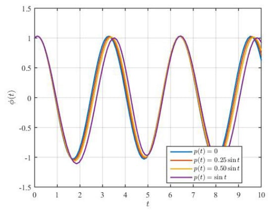
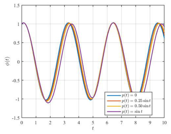
To complement the continuous-limit representation in Example 1, we illustrate the influence of the potential function $p\left(t\right)$ on the solution profile. For the fixed initial data $\varphi \left(0\right)=1$, ${\varphi }^{\prime }\left(0\right)=0.5$, and the spectral parameter $\eta =2$, the problem is considered for $p\left(t\right)=0$, $0.25sint$, $0.50sint$, and $sint$. For the numerical computation, the continuous problem was solved on the interval $[0,10]$ by rewriting the second-order equation as the first-order system

$${\varphi }^{\prime }=z,z^{\prime }=\left(p\left(t\right)-{\eta }^2\right)\varphi .$$

The resulting initial-value problem was integrated using the MATLAB ode45 solver with its default adaptive step-size and error-control settings. The corresponding solutions are shown in Figure 3.

Figure 3. Continuous-limit solutions $\varphi \left(t\right)$ on $[0,10]$ computed using the MATLAB ode45 solver for $\varphi \left(0\right)=1$, ${\varphi }^{\prime }\left(0\right)=0.5$, $\eta =2$, and $p\left(t\right)=Asint$ with $A=0,0.25,0.50,$ and 1.

Figure 3 shows that the potential term modifies both the amplitude and the oscillatory behavior of the solution, whereas the zero-potential case provides the corresponding free reference solution. This numerical comparison is consistent with the potential-dependent Volterra representation obtained in Example 1.

4. Discussion of the Diamond-$\mathit{\alpha }$ Spectral Structure

The results obtained in the preceding section reveal several differences between the diamond-$\alpha$ formulation and the classical Sturm–Liouville framework. The most significant distinction arises from the simultaneous presence of the forward and backward dynamic components. Unlike the purely delta or purely nabla settings, the combined operator produces additional terms when integration by parts is applied. These contributions appear explicitly in the generalized Green identity through the remainder term $R_{\alpha }$.

The main structural differences between the classical and time scale formulations are summarized in Table 1.

Table 1. Structural comparison of the spectral formulations.

Framework	Derivative Structure	Diamond-$\mathit{\alpha }$ Defect	Orthogonality Condition
Continuous	${\displaystyle \frac{d}{dt}}$	Absent	Boundary term vanishes
Delta	$\Delta$	N/A	Delta formulation
Nabla	∇	N/A	Nabla formulation
Diamond-$\alpha$	$\alpha \Delta +(1-\alpha )\nabla$	$R_{\alpha }$	$B_{{\diamond }_{\alpha }}+R_{\alpha }=0$

• Numerical scope and limitations. The numerical experiments presented above are designed to illustrate the graininess dependence of the defect structure established analytically in Section 3. Direct numerical computation of eigenvalues and eigenfunctions for varying $\alpha$ and $\nu$ would require a specific homogeneous endpoint realization of the diamond-$\alpha$ spectral expression. In particular, on a uniform time scale the iterated diamond-$\alpha$ derivative involves shifted values extending beyond the standard three-point stencil, so that additional endpoint closure conditions are required for a discrete matrix eigenvalue problem.

Since the prescribed conditions (2) and (3) considered in the present work do not provide such a homogeneous endpoint realization, we do not introduce additional artificial boundary conditions solely for numerical spectral computation. The present numerical analysis is therefore restricted to quantities directly supported by the analytical framework, in particular the behavior of the defect term as the graininess decreases. A systematic numerical study of the eigenvalue and eigenfunction dependence on $\alpha$ and $\nu$, under appropriately specified homogeneous endpoint realizations, is left for future work.

• Influence of the Weighting Parameter $\mathit{\alpha }$ on the Spectral Structure

The parameter $\alpha$ plays a structural role in the diamond-$\alpha$ spectral problem, since it determines the relative contribution of the forward and backward dynamic components. This dependence becomes particularly visible in the generalized Green identity. Two coefficients occurring in the boundary contribution are

$${\kappa }_{\alpha }=1-2\alpha +2{\alpha }^2$$

and

$$\beta \alpha =\alpha (1-\alpha ).$$

Their behavior provides additional information about the interaction between the delta and nabla parts of the operator.

The coefficient $\beta \alpha$ attains its maximum value $1/4$ at $\alpha =1/2$ and tends to zero as $\alpha \to 0^{+}$ or $\alpha \to 1$. In contrast, ${\kappa }_{\alpha }$ attains its minimum value $1/2$ at $\alpha =1/2$ and approaches unity as $\alpha \to 0^{+}$ or $\alpha \to 1$. Thus, the balanced choice $\alpha =1/2$ gives the strongest contribution of the mixed boundary component measured by $\alpha (1-\alpha )$, whereas the coefficient multiplying the principal Wronskian contribution becomes smallest.

This observation distinguishes the intermediate diamond-$\alpha$ regime from the limiting one-sided cases. As $\alpha$ approaches 1, the delta component becomes dominant and the mixed coefficient $\alpha (1-\alpha )$ tends to zero. Formally, the analogous behavior occurs toward the nabla endpoint when $\alpha$ approaches 0. For interior values of $\alpha$, however, both differentiation directions participate in the spectral structure, and their interaction is reflected in the additional terms appearing in the Green-type relation.

The symmetric value $\alpha =1/2$ is therefore of particular interest, but it should not be interpreted as a case in which all additional diamond contributions disappear. Indeed, the special-case analysis given above shows that the remainder term may remain nonzero even when the forward and backward components receive equal weights. Hence, balancing the two dynamic directions does not automatically restore the classical Sturm–Liouville structure.

These observations indicate that $\alpha$ acts as more than a simple interpolation parameter. Its value changes the relative weighting of the terms entering the boundary and remainder contributions and therefore affects the conditions under which symmetry and orthogonality can be established. This parameter-dependent structure provides a natural motivation for further investigating the variation of eigenvalues and eigenfunctions with respect to $\alpha$.

This observation has direct consequences for the spectral properties of the problem. In the classical continuous setting, the vanishing of the boundary form is sufficient to obtain the usual orthogonality relation for eigenfunctions corresponding to distinct eigenvalues. In the diamond-$\alpha$ framework, however, the remainder contribution must also be taken into account. Consequently, orthogonality is obtained under a compatibility condition involving both the boundary term and $R_{\alpha }$. This indicates that the combined forward–backward structure modifies the mechanism by which symmetry and orthogonality are established.

The parameter $\alpha$ also provides a natural connection between different dynamic regimes. At $\alpha =1$, the diamond-$\alpha$ operator reduces to the delta operator, whereas the limiting regime $\alpha \to 0^{+}$ formally approaches the nabla setting. Intermediate values of $\alpha$ incorporate both directions of differentiation and may therefore be interpreted as describing a continuous transition between the two dynamic structures. From the spectral point of view, this transition is reflected in the additional terms present in the Green identity and the associated integral relations.

At the level of the diamond-$\alpha$ differential expression and the coefficients appearing in the generalized Green identity, the dependence on $\alpha$ is continuous. Indeed,

$$f^{{\diamond }_{\alpha }}=\alpha f^{\Delta }+(1-\alpha )f^{\nabla },$$

while

$${\kappa }_{\alpha }={\alpha }^2+{(1-\alpha )}^2,\alpha (1-\alpha ),$$

are continuous functions of $\alpha$. Hence, for functions for which both the delta and nabla derivatives exist, the formal diamond-$\alpha$ structure varies continuously with the weighting parameter. In particular, $\alpha =1$ yields the delta formulation, whereas the limit $\alpha \to 0^{+}$ approaches the corresponding nabla formulation.

This continuity statement concerns the differential expression and the coefficients entering the Green-type identities. It should not be interpreted as establishing continuity of individual eigenvalues or eigenfunctions with respect to $\alpha$. Such spectral continuity would require additional assumptions and a separate perturbation analysis, which is beyond the scope of the present work.

The dense time scale limit provides an important consistency check. When $\mathbb{T}=\mathbb{R}$, the forward and backward jump operators coincide with the identity mapping and the additional remainder terms disappear. More generally, Proposition 2 and Corollary 1 provide a quantitative description of this transition. For a family of regular uniform time scales with graininess $\nu \to 0$, and provided that the relevant norms remain uniformly bounded, the defect term satisfies

$$R_{\alpha }(u,v)=O\left(\nu \right).$$

Thus, under the stated assumptions, the magnitude of the remainder term is bounded by a quantity of order $\nu$. Consequently, the generalized Green structure approaches its dense counterpart as the mesh becomes finer. This provides a quantitative connection between the diamond-$\alpha$ formulation on uniform time scales and the classical continuous Sturm–Liouville setting.

This dense-limit behavior also has a direct spectral consequence. If the boundary form vanishes for eigenfunctions ${\varphi }_1$ and ${\varphi }_2$ corresponding to distinct eigenvalues, Proposition 3 gives

$$\left|{⟨{\varphi }_1,{\varphi }_2⟩}_{{\diamond }_{\alpha }}\right|={\displaystyle \frac{|R_{\alpha }({\varphi }_1,{\varphi }_2)|}{|{\lambda }_1-{\lambda }_2|}}.$$

Hence, under the uniform boundedness assumptions of Proposition 2 and a spectral gap uniformly separated from zero,

$${⟨{\varphi }_1,{\varphi }_2⟩}_{{\diamond }_{\alpha }}=O\left(\nu \right).$$

Thus, although exact orthogonality on a non-dense time scale requires the compatibility condition of Theorem 4, eigenfunctions associated with uniformly separated distinct eigenvalues become asymptotically orthogonal as the graininess tends to zero, provided the boundary contribution vanishes.

These observations suggest that the diamond-$\alpha$ formulation should not be regarded merely as a formal combination of the delta and nabla theories. Instead, the interaction between the two dynamic components generates a distinct spectral structure whose properties depend on the underlying time scale, the weighting parameter, and the compatibility conditions imposed on the associated functions.

• Role of the uniform time scale assumption. The restriction to regular uniform time scales is essential for some of the quantitative conclusions obtained in this work. In particular, the constant-graininess relations used to estimate the shift differences are required in the derivation of the $O\left(\nu \right)$ bound for the defect term and, consequently, in the dense-limit asymptotic orthogonality result. The corresponding simplifications in the balanced case $\alpha =1/2$ also make explicit use of the uniform shift structure.

By contrast, several algebraic features of the diamond-$\alpha$ calculus, including its representation as a weighted combination of delta and nabla derivatives and the associated integration-by-parts mechanism, suggest that analogous Green-type identities may be formulated on broader classes of regular time scales. On a nonuniform time scale, however, the constant parameter $\nu$ must be replaced by the local forward and backward graininess functions, and the defect estimates would require additional control of these quantities. Therefore, the present results are stated only for the uniform setting, and no general extension to arbitrary regular time scales is claimed here.

5. Conclusions

In this study, a Sturm–Liouville problem involving the diamond-$\alpha$ derivative has been investigated on regular uniform time scales. The analysis shows how the simultaneous contribution of the delta and nabla operators can be incorporated into the spectral structure through the diamond-$\alpha$ framework.

The main spectral features of the problem have been investigated. In particular, a conditional linear-dependence result has been obtained for solutions associated with the same eigenvalue under the stated uniqueness assumption, while orthogonality of eigenfunctions corresponding to distinct eigenvalues has been established under an appropriate compatibility condition involving the boundary form and the remainder term. A generalized Green identity has also been derived, yielding symmetry on a linear realization of the operator whenever both the remainder term and the associated boundary form vanish for all functions in its domain.

The remainder term arising from diamond-$\alpha$ integration by parts has been characterized as a skew-symmetric defect form and quantitatively estimated. For families of regular uniform time scales with graininess $\nu \to 0$, the estimate $R_{\alpha }(u,v)=O\left(\nu \right)$ holds under the stated uniform boundedness assumptions. When the boundary form vanishes and the spectral gap remains uniformly separated from zero, this estimate yields asymptotic orthogonality in the dense-limit regime. A generalized integral identity has also been obtained, explicitly retaining the additional contribution generated by the diamond-$\alpha$ structure.

These results show that the direct diamond-$\alpha$ formulation possesses a spectral structure that differs from that of the classical continuous setting through the defect term $R_{\alpha }$. The present analysis is restricted to regular uniform time scales and relies on the stated uniqueness and compatibility assumptions. Extensions to more general time scales and boundary conditions, as well as eigenvalue asymptotics, completeness, inverse spectral problems, and numerical approximation, constitute natural directions for future research.

References

- Hilger, S. Ein Maßkettenkalkül mit Anwendung auf Zentrumsmannigfaltigkeiten. Ph.D. Thesis, Universität Würzburg, Würzburg, Germany, 1988. [Google Scholar]
- Bohner, M.; Peterson, A. Dynamic Equations on Time Scales, an Introduction with Applications; Birkhäuser: Boston, MA, USA, 2001. [Google Scholar]
- Bohner, M.; Peterson, A. Advances in Dynamic Equations on Time Scales; Birkhäuser: Boston, MA, USA, 2003. [Google Scholar]
- Bohner, M.; Georgiev, S. Multivariable Dynamic Calculus on Time Scales; Springer: Cham, Switzerland, 2016. [Google Scholar]
- Guseinov, G.S.; Kaymakcalan, B. Basics of Riemann Δ and ∇ integration on time scales. J. Differ. Equ. Appl. 2002, 8, 1001–1017. [Google Scholar] [CrossRef] [Scilit]
- Caputo, M.C. Time scales: From nabla calculus to delta calculus and vice versa via duality. Int. J. Differ. Equ. 2010, 5, 25–40. [Google Scholar]
- Atici, F.M.; Biles, D.C.; Lebedinsky, A. An application of time scales to economics. Math. Comput. Model. 2006, 43, 718–726. [Google Scholar] [CrossRef] [Scilit]
- Guseinov, G.S. Integration on time scales. J. Math. Anal. Appl. 2003, 285, 107–127. [Google Scholar] [CrossRef] [Scilit]
- Agarwal, R.P.; Bohner, M. Basic calculus on time scales and some of its applications. Results Math. 1999, 35, 3–22. [Google Scholar] [CrossRef] [Scilit]
- Sheng, Q.; Fadag, M.; Henderson, J.; Davis, J.M. An exploration of combined dynamic derivatives on time scales and their applications. Nonlinear Anal. Real World Appl. 2006, 7, 395–413. [Google Scholar] [CrossRef] [Scilit]
- Rogers, J.W., Jr.; Sheng, Q. Notes on the diamond dynamic derivative on time scales. J. Math. Anal. Appl. 2007, 326, 228–241. [Google Scholar] [CrossRef] [Scilit]
- Celik, O.F.; Yantır, A. Diamond-α Dynamic Equations on Time Scales. Master’s Thesis, Yaşar University, Bornova, Türkiye, 2016. [Google Scholar]
- Atasever, N. On Diamond Alpha Dynamic Equations and Inequalities. Master’s Thesis, Georgia Southern University, Statesboro, GA, USA, 2011. [Google Scholar]
- Mozyrska, D.; Torres, D.F.M. A study of diamond alpha dynamic equations on regular time scales. Afr. Diaspora J. Math. 2009, 8, 35–47. [Google Scholar]
- Malinowska, A.B.; Torres, D.F.M. On the diamond alpha Riemann integral and mean value theorems on time scales. Dyn. Syst. Appl. 2009, 18, 469–482. [Google Scholar]
- Mozyrska, D.; Torres, D.F. Diamond-alpha polynomial series on time scales. arXiv 2008, arXiv:0805.0274. [Google Scholar]
- Brito da Cruz, A.M.; Martins, N.; Torres, D.F. The diamond integral on time scales. Bull. Malays. Math. Sci. Soc. 2015, 38, 1453–1462. [Google Scholar] [CrossRef] [Scilit]
- Wang, C.; Agarwal, R.P. ⋄α— Measurability and Combined Measure Theory on Time Scales. In Combined Measure and Shift Invariance Theory of Time Scales and Applications; Springer International Publishing: Cham, Switzerland, 2022; pp. 117–195. [Google Scholar]
- Qin, G.; Wang, C. Lebesgue–Stieltjes combined ⋄α- measure and integral on time scales. Rev. Real. Acad. Cienc. Exactas Fis. Nat.-A Mat. 2021, 115, 50. [Google Scholar] [CrossRef] [Scilit]
- Kayar, Z.; Kaymakçalan, B. Applications of the novel diamond alpha Hardy–Copson type dynamic inequalities to half linear difference equations. J. Differ. Equ. Appl. 2022, 28, 457–484. [Google Scholar] [CrossRef] [Scilit]
- Kayar, Z.; Kaymakcalan, B. Extensions of Diamond alpha Hardy-Copson type dynamic inequalities and their applications to oscillation theory. Dyn. Syst. Appl. 2021, 30, 1180–1210. [Google Scholar] [CrossRef] [Scilit]
- Bohner, M.; Matthews, T.; Tuna, A. Diamond-alpha Grüss type inequalities on time scales. Int. J. Dyn. Syst. Differ. Equ. 2011, 3, 234–247. [Google Scholar] [CrossRef] [Scilit]
- Anderson, D.R. The discrete diamond-alpha imaginary ellipse and Hyers–Ulam stability. Int. J. Differ. Equ. 2019, 14, 25–38. [Google Scholar] [CrossRef] [Scilit]
- Anderson, D.R.; Onitsuka, M. Equilibrium Stability for the Discrete Diamond–Alpha Operator. Bull. Malays. Math. Sci. Soc. 2023, 46, 15. [Google Scholar] [CrossRef] [Scilit]
- Amster, P.; De Napoli, P.; Pinasco, J.P. Detailed asymptotic of eigenvalues on time scales. J. Differ. Equ. Appl. 2009, 15, 225–231. [Google Scholar] [CrossRef] [Scilit]
- Huseyinov, A.; Bairamov, E. On expansions in eigenfunctions for second order dynamic equations on time scales. Nonlinear Dyn. Syst. Theory 2009, 9, 77–88. [Google Scholar]
- Guseinov, G.S. Self-adjoint boundary value problems on time scales and symmetric Green’s functions. Turk. J. Math. 2005, 29, 365–380. [Google Scholar]
- Rynne, B.P. L2 spaces and boundary value problems on time scales. J. Math. Anal. Appl. 2007, 328, 1217–1236. [Google Scholar] [CrossRef] [Scilit]
- Chatzarakis, G.E.; Jadlovska, I. Oscillations in difference equations with several arguments using an iterative method. Filomat 2018, 32, 255–273. [Google Scholar] [CrossRef] [Scilit]
- Agarwal, R.P.; Bohner, M.; Wong, J.Y. Sturm-Liouville eigenvalue problems on time scales. Appl. Math. Comput. 1999, 99, 153–166. [Google Scholar] [CrossRef] [Scilit]
- Guseinov, G.S. Eigenfunction expansions for a Sturm-Liouville problem on time scales. Int. J. Differ. Equ. 2007, 2, 93–104. [Google Scholar]
- Bairamov, E.; Aygar, Y.; Koprubasi, T. The spectrum of eigenparameter-dependent discrete Sturm-Liouville equations. J. Comput. Appl. Math. 2011, 235, 4519–4523. [Google Scholar] [CrossRef] [Scilit]
- Özkan, A.S. Sturm-Liouville operator with parameter-dependent boundary conditions on time scales. Electron. J. Differ. Equ. 2017, 212, 1–10. [Google Scholar]
- Allahverdiev, B.P.; Eryilmaz, A.; Tuna, H. Dissipative Sturm-Liouville operators with spectral parameter in the boundary condition on bounded time scales. Electron. J. Differ. Equ. 2017, 95, 1–13. [Google Scholar]
- Erbe, L.; Mert, R.; Peterson, A. Spectral properties of diffusion equation on time scales. Appl. Math. Comput. 2012, 218, 7671–7678. [Google Scholar]
- Aygar, Y.; Bohner, M. On the spectrum of eigenparameter-dependent quantum difference equations. Appl. Math. Inf. Sci. 2015, 9, 1725–1729. [Google Scholar]
- Gulsen, T.; Yilmaz, E. Spectral theory of Dirac System on time scales. Appl. Anal. 2017, 96, 2684–2694. [Google Scholar] [CrossRef] [Scilit]
- Levitan, B.M.; Sargsjan, I.S. Introduction to Spectral Theory, Selfadjoint Ordinary Differential Operators; American Mathematical Society: Providence, RI, USA, 1970. [Google Scholar]
- Gulsen, T.; Yar, A.Ç.; Yilmaz, E. Diamond-type Dirac dynamic system in mathematical physics. Symmetry 2024, 16, 318. [Google Scholar] [CrossRef] [Scilit]
Disclaimer/Publisher’s Note: The statements, opinions and data contained in all publications are solely those of the individual author(s) and contributor(s) and not of MDPI and/or the editor(s). MDPI and/or the editor(s) disclaim responsibility for any injury to people or property resulting from any ideas, methods, instructions or products referred to in the content. |
© 2026 by the authors. Licensee MDPI, Basel, Switzerland. This article is an open access article distributed under the terms and conditions of the Creative Commons Attribution (CC BY) license.