


Abstract
In this work, we focus on deriving the absolute moments of the generalised hyperbolic (GH) distribution through its mean–variance mixture structure. Conditioning on the GIG mixing variable reduces the problem to Gaussian moment calculations and known GIG power moments, avoiding direct integration with Bessel functions. The variance-gamma (VG), normal inverse Gaussian (NIG), hyperbolic, Normal, and Student’s t distributions emerge as natural special or limiting cases of the generalised hyperbolic family. This approach offers a substantially simpler and more transparent derivation, facilitating both implementation and verification.
Keywords:
absolute moment; generalised hyperbolic distribution; normal inverse Gaussian distribution; raw moment; variance-gamma distribution MSC:
92D25; 37H15; 60H10; 60J60
1. Introduction
The problem of obtaining explicit expressions for absolute moments is a classical and well-motivated one in distribution theory. Classical results exist for the normal distribution (Winkelbauer [1]), the generalised hyperbolic (GH) family (Barndorff-Nielsen & Stelzer [2]), and the multivariate normal distribution, among others. In particular, Barndorff-Nielsen and Stelzer [2] made two main contributions: (i) They derived explicit formulae for the absolute moments of the GH family and its important subclass, the normal inverse Gaussian (NIG) distribution, with expressions given in terms of series of Bessel functions and linked to the moments of their symmetric (zero-skewness) counterparts. (ii) They investigated the scaling behaviour of NIG Levy processes by computing the logarithmic derivative of centred absolute moments with respect to time, revealing that these processes exhibit approximate rather than exact scaling and providing insights into this phenomenon. Subsequently, Gaunt [3] obtained new closed-form formulas for moments (for odd k) and absolute moments (for ) of the variance-gamma (VG) distribution VG, which in turn led to new formulas for the moments and absolute moments of the product of two correlated zero-mean normal random variables. The variance-gamma distribution is a flexible four-parameter family widely used in finance, insurance, and statistics. Although its ordinary moments are well known, explicit expressions for its absolute moments, which are crucial for Markov inequalities, Berry–Esseen-type bounds, and scaling analyses, had been lacking for the fully asymmetric case. Gaunt [4] derived the closed-form expressions for the absolute moments of the four-parameter variance-gamma (VG) distribution VG for , odd integers, and , respectively. Its results are not only of theoretical interest, but they also offer practical tools for estimation, approximation, and further probabilistic modelling, and the future directions Gaunt identified show that this work serves as a solid foundation for ongoing research in distribution theory and its applications. Scott et al. [5] provided the first computationally efficient recursive framework for calculating the moments of the generalised hyperbolic (GH) distribution, expressing them as finite sums of modified Bessel function ratios. This advancement resolved the limitations of earlier integral-based methods and enabled stable computation of higher-order statistics across the entire GH family.
Nevertheless, the existing closed-form expressions for the generalised hyperbolic class, while mathematically rigorous, are often encumbered by the analytic complexity of their Bessel-function series representations. Such series, though explicit, can be computationally demanding for high-order moments or specific parameter regimes, and they do not always readily reveal the role of the individual shape, skewness, and scaling parameters in determining the moment structure. Moreover, the established literature has primarily focused either on symmetric subclasses or on particular limiting cases, leaving the full generality of the GH family, particularly with respect to both raw and central absolute moments under arbitrary parametrisation, less systematically addressed in a unified framework.
The purpose of this paper was to provide a unified formula for absolute moments of the GH distribution, including absolute raw moments and absolute central moments, with real-valued orders, based on its mean–variance Gaussian mixture representation. This hierarchical perspective, which interprets the GH distribution as a normal variance–mean mixture driven by a generalised inverse Gaussian (GIG) mixing distribution, offers a twofold advantage. First, it reduces the problem of moment calculation to that of evaluating moments of the GIG mixing variable, for which explicit and well-structured formulae are available in terms of modified Bessel functions of the second kind. Second, and more importantly, this representation yields moment expressions that are not only fully explicit but also structurally transparent: they separate the contributions of the location, skewness, and tail-weight parameters in a tractable manner. As a result, our derivation provides a direct probabilistic interpretation of each moment component, facilitates efficient numerical implementation across the entire GH parameter space, and generalises several earlier results as special cases. Furthermore, by encompassing both raw and central absolute moments in a coherent framework, our results offer a more comprehensive toolkit for moment-based inference, tail-risk quantification, and the refined scaling analysis of GH-driven Levy processes beyond the NIG subclass.
The remainder of this paper is organised as follows. Section 2 provides preliminaries, reviewing the GH distribution and its GIG mixture representation and setting up the basic notation. Section 3 presents the main theoretical results, namely the unified closed-form expressions for both raw and central absolute moments. Section 4 discusses some special cases. Section 5 gives a numerical analysis of the convergence of the series. Section 6 concludes the paper.
- Notation. For later use, we will require some special functions, which can be found in the work of Olver et al. [6] or Abramowitz and Stegun [7].
The generalised hypergeometric function is defined by
where is the Pochhammer symbol:
In particular, is defined as
The Kummer confluent hypergeometric function is
The Gaussian hypergeometric function is
The modified Bessel function of the second kind is
An integral representation of it is
Asymptotically,
Regarding large-order asymptotics, for fixed z, as ,
The generalised Laguerre polynomials are defined by
Equivalently,
Rodrigues’ formula reads
2. Generalised Hyperbolic Distribution
This section provides preliminaries, reviewing the GH distribution and its limiting or particular cases. The generalised hyperbolic (GH) distribution, introduced by Barndorff-Nielsen ([8,9]), is a flexible family of distributions that arises as a normal variance–mean mixture with a generalised inverse Gaussian (GIG) mixing variable. A random variable X from this family has the density
where , , and is the modified Bessel function of the second kind. Here, the parameter constraints are , , and . Under this parametrisation, the GH distribution is denoted by
The characteristic function of the GH distribution is given by
It is straightforward to show that the random variable can be represented as a mean–variance Gaussian mixture:
where , , a generalised inverse Gaussian distribution, Z and W are independent, is a location parameter, is a skewness parameter, is a scale parameter, is a shape parameter, and and are parameters of the GIG mixing distribution. The density of
is given by
The p-th moment of W is (Jørgensen [10], Ch. 1; Barndorff-Nielsen [8])
When , we recover the standard GH parametrisation . For a general overview over normal variance–mean mixtures, see Barndorff-Nielsen et al. [11]. Yu [12] investigated the shape properties of normal variance–mean mixtures, focusing on conditions that ensure density unimodality and log-concavity. For the research background and the latest advances on generalised hyperbolic (GH) distributions, see the work of Jiang, Nadarajah, and Hitchen [13], which systematically surveys the GH family. For a comprehensive account of the variance-gamma distribution, its distributional theory, estimation methods and applications, we refer readers to Fischer, Gaunt, and Sarantsev [14].
The GH distribution contains many known distributions as limiting or particular cases. These include the variance-gamma (VG), normal inverse Gaussian (NIG), hyperbolic, Normal, and Student’s t distributions. Its flexibility arises from parameters , , , , and , which jointly control tail heaviness, skewness, kurtosis, and scale. This has established the GH distribution as a versatile modelling framework with applications spanning finance, physics, geology, and statistics. Foundational contributions include the work of Barndorff-Nielsen & Blæsild [15]; comprehensive treatments are given by Eberlein & von Hammerstein [16]; and financial applications can be found in the work of Madan and Seneta [17] and Aas & Haff [18]. Some recent results can be found from Barndorff-Nielsen and Stelzer [2], Scott et al. [5], Gaunt [3], Fischer, Gaunt and Sarantsev [14], and Gaunt [4].
We now summarize important special cases obtained by fixing specific parameter values or by considering limiting regimes.
2.1. The Normal Inverse Gaussian Distribution
When , the generalised hyperbolic distribution reduces to the normal-inverse Gaussian (NIG) distribution (see, e.g., Aas & Haff [18], Paolella [19]). Using the identity , the CF reduces to
The corresponding probability density function is
This density is valid for all , with parameters , , , , and .
2.2. The Hyperbolic Distribution
Setting yields the hyperbolic distribution, which arises from a GIG mixing law with shape parameter and was originally introduced by Barndorff-Nielsen [8]. The CF of X reads
where is the modified Bessel function of the third kind, and the parameters satisfy , , , and .
The corresponding probability density function is
where , , , , and .
2.3. Symmetric GH
Setting in the GH density (1) yields the symmetric GH distribution (see Barndorff-Nielsen [8]), for which the mean–variance mixture simplifies to
so that X is symmetric about . The CF becomes real and even:
The corresponding probability density function is
where the parameters satisfy
and denotes the modified Bessel function of the second kind.
2.4. Variance-Gamma Distribution
For , the limit (i.e., ) reduces the GH distribution to the variance-gamma (VG) distribution. This corresponds to replacing the GIG mixing distribution with a gamma distribution, so that X becomes a variance–mean mixture of a normal distribution with a gamma-distributed mixing variable.
Using the small-argument asymptotics as , the CF converges to
This is the CF of the variance-gamma distribution with shape parameter . Its probability density function is
The parameters satisfy
and denotes the modified Bessel function of the second kind. See, e.g., Fischer, Gaunt and Sarantsev [14], Gaunt [4].
2.5. GH Skewed t-Distribution
Several definitions have been presented in the literature that can be regarded as competing skew Student’s t-distributions. Here, we take the skew Student’s t-distribution as a limiting case of the GH distribution (see, e.g., Aas & Haff [18]). Let (equivalently ) and set . The limiting distribution is the generalised hyperbolic skewed t. The probability density function is
for all , with parameters
When , it degenerates to Student’s t-distribution.
For quick reference, the main special cases are collected in Table 1.
Table 1.
Special cases of the GH characteristic function. Here, .
3. Absolute Moment of GH Distribution
Motivated by the recent work of Kirkby, Nguyen, and Nguyen [20], who utilized a normal-gamma mixture representation to unify moment derivations for Student’s t-distribution, we adopt the same technique in this section to derive the absolute raw and central moments of the GH distribution.
3.1. Absolute Central Moments
Theorem 1.
Let . Then, for , the absolute moment of the GH distribution is given by
with , .
Proof.
Conditional on ,
where the GIG density is (, ):
Define independently of W. Then,
Consequently, for any for which the expectation exists,
and taking expectations gives
We first evaluate the inner absolute moment of the normal variable. For and any constant , the absolute moment of is known to be (see, e.g., Winkelbauer [1])
where is Kummer’s confluent hypergeometric function. Substituting yields
Inserting (16) into (14) produces the following closed-form formula:
for , where is the confluent hypergeometric function.
Expand the hypergeometric function as a power series:
where denotes the Pochhammer symbol.
By substituting this expansion into the expectation and invoking the dominated convergence theorem to justify the interchange of sum and integral, we obtain
Using (5),
Substituting back into the expectation:
Combining the powers gives
Finally, inserting this result into (17) yields
which is (13). □
Remark 1.
Since and , Equation (13) can be rewritten as
Remark 2
(Absolute convergence). The series
converges absolutely for all and admissible parameters , . This follows from two observations: (i) the coefficients are the Maclaurin coefficients of the entire function ; (ii) the Bessel ratio decays exponentially as by the large-order asymptotics (see [21]). Equivalently, convergence is guaranteed by the finiteness of under the GH law, since iff for .
3.2. Absolute Raw Moments
In numerous applications, one is often interested in the absolute moments about the origin, , rather than in the central moments.
Theorem 2.
Assume that . Then, for , the absolute moment of X is
Proof.
Recall the mean–variance Gaussian mixture representation
Hence,
Conditional on W and using the law of total expectation,
Given , the inner expectation is the absolute moment of a normal random variable with mean and variance . Applying the standard Formula (15) with and scale gives
Substituting (22) into (21) yields the unified formula for the origin absolute moments:
Let
Expand the confluent hypergeometric function:
Using the trinomial expansion,
Thus,
Using (5),
Finally, inserting this result into (23) yields (20). □
Remark 3.
The series
converges absolutely for every and for all admissible parameters with , . This follows from three facts:
- 1.
- The outer coefficient is the Maclaurin coefficient of the entire confluent hypergeometric function ; hence, the outer series has infinite radius of convergence.
- 2.
- The inner multinomial sum is a finite polynomial in n and thus introduces no new divergence.
- 3.
- For fixed λ and , the Bessel ratio decays exponentially as by the large-order asymptotics .
4. Special Cases
4.1. Absolute Moments of the NIG Distribution
Let . Then,
reduces to an inverse Gaussian distribution. Let with density (6). Then, for ,
where is the Pochhammer symbol. This agrees with the known absolute moment formulas for NIG distributions used in the study of approximate scaling of NIG Lévy processes in the special case ; see, e.g., Barndorff-Nielsen and Stelzer [2].
In particular, when ,
For ,
where is the Pochhammer symbol.
In particular, when , only the term survives in the binomial expansion, and the above expression reduces to the earlier formula for .
4.2. Absolute Moments of the Hyperbolic Distribution
Let X follow the hyperbolic distribution with density (7). Then, for ,
In the symmetric case , this reduces to
For ,
Here, denotes the Pochhammer symbol, is the modified Bessel function of the second kind, and the summation indices and k are non-negative integers satisfying .
4.3. Absolute Moments of the Symmetric GH Distribution
Setting in the GH model yields the symmetric GH law , where . The absolute central moments are given by
and the absolute raw moments are given by
In the fully symmetric case , this reduces to
4.4. Absolute Moments of the VG Distribution
For , letting reduces the GH distribution to the variance-gamma (VG) distribution (11).
For any real number , the r-th absolute central moment is given by the closed-form expression:
If the distribution is symmetric, i.e., , Formula (24) simplifies to
The absolute raw moments are given by
where .
When , Equation (25) reduces to
Additionally, if , the hypergeometric function equals 1, giving
This matches the known result for the symmetric variance-gamma distribution (see Gaunt [3]).
4.5. Absolute Moments of the GH Skewed t Distribution
Let X follow the GH skewed t distribution with density, corresponding to the GH limit , . Let W follow an inverse-gamma distribution with shape and scale , and write . For , the absolute central moments are given by
and the absolute raw moments are given by
For , this reduces to
5. Numerical Convergence Analysis
To examine the numerical convergence of the series in Theorems 1 and 2, we compare the truncated sums with direct numerical integration. Let denote the nth summand in (13), let
and let , where
is the prefactor in (13). The reference value and the relative error are
The truncation orders are defined by
For a terminating series, the last non-zero order is recorded. The maximum truncation order is , and .
5.1. Absolute Central Moments
In Table 2, and in all cases. Unless otherwise stated, , , and . Sets A–C vary , Sets D and E vary , Set F changes , and Set G changes the moment order.
Table 2.
Numerical convergence for Theorem 1.
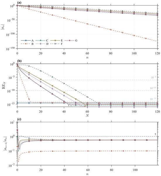
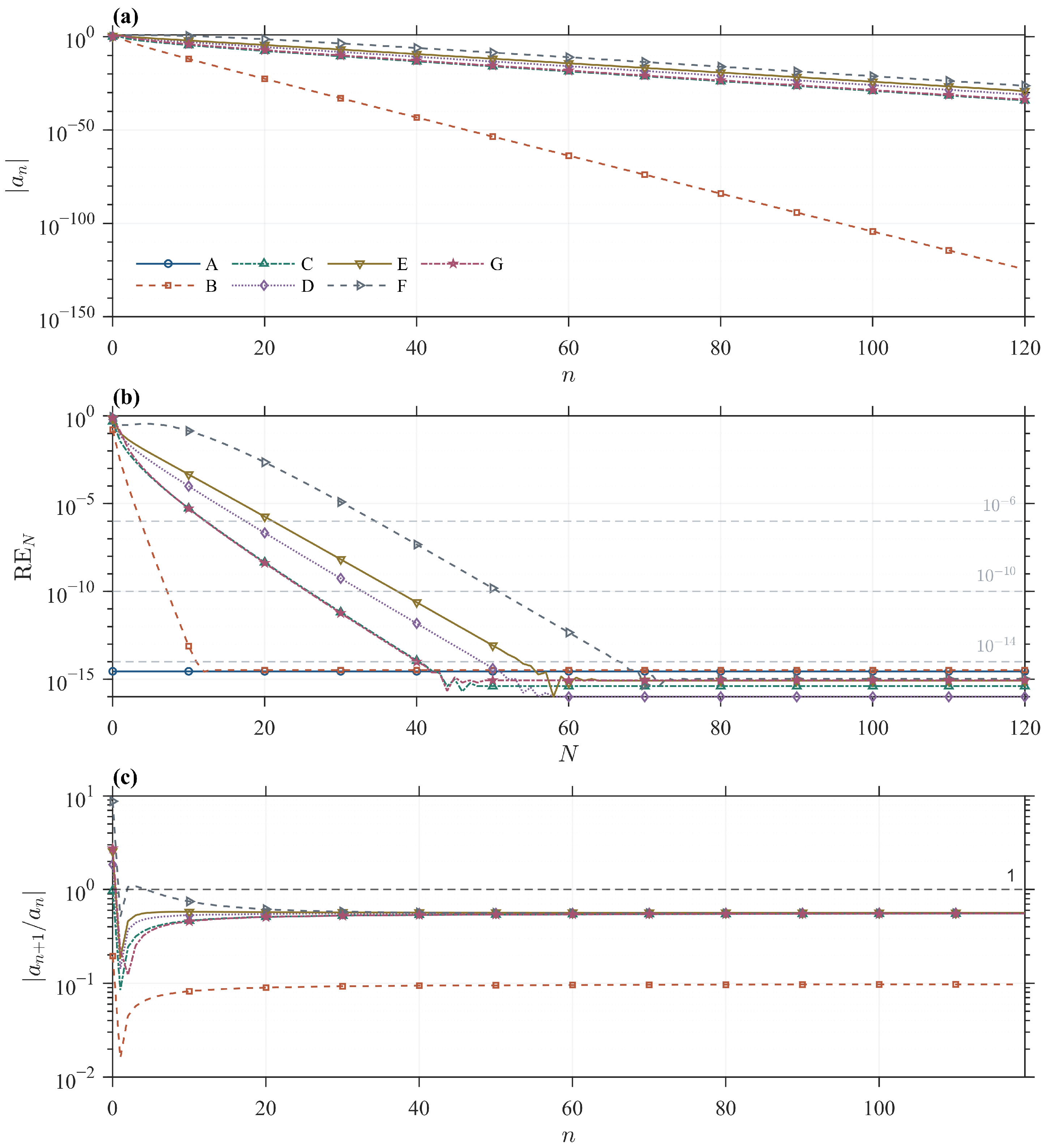
The series in Theorem 1 converges rapidly. Increasing from to increases from 12 to 42, while the corresponding orders for Sets D–F are 51, 56, and 69. For the non-terminating sets, the error-based truncation orders are consistently 1–2 steps below the corresponding values, indicating that the term-based criterion is conservative in these numerical tests. At , the truncated values agree with the numerical integration values to order or smaller. Figure 1 shows the decay of the summands, the relative errors and the consecutive-term ratios, giving a direct numerical verification of (13).
Figure 1.
Numerical convergence for Theorem 1. (a) ; (b) ; (c) .
5.2. Absolute Raw Moments
For Theorem 2, let denote the complete nth outer summand in (20), including the finite sum over , and replace with in (26). Here,
In Table 3, , , , , and .
Table 3.
Numerical convergence for Theorem 2.
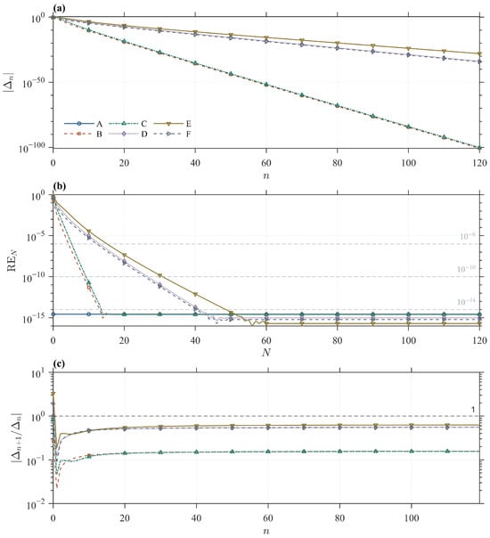
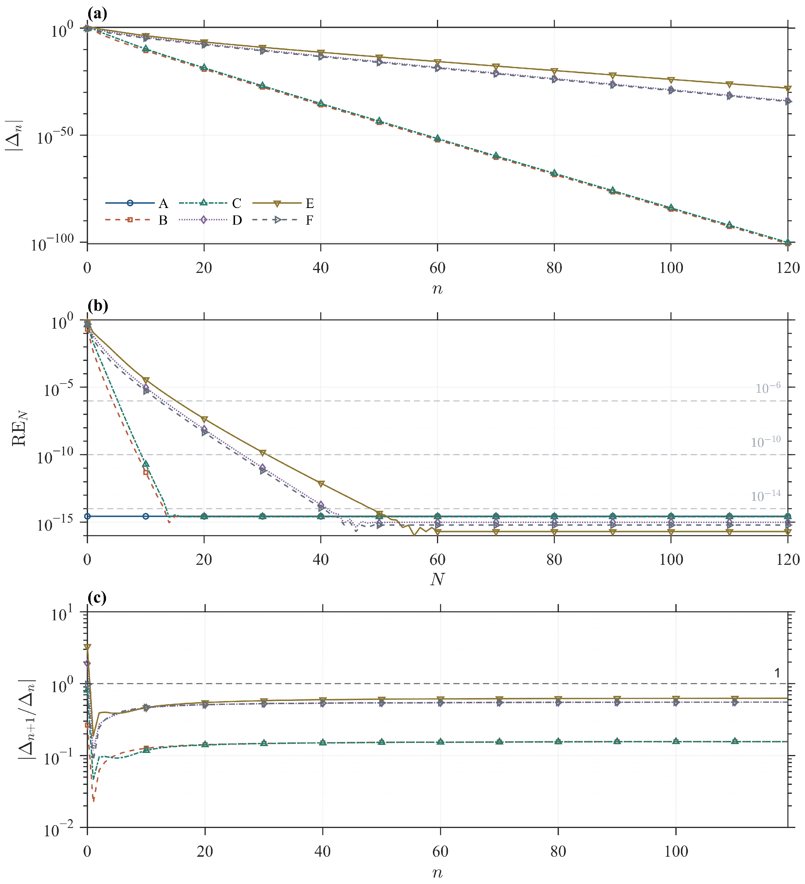
The same pattern is found for Theorem 2. At the level, is 15 for Sets B and C, 43 for Set D, 51 for Set E, and 42 for Set F. The truncated values again agree with the numerical integration values to order or smaller. Figure 2 gives the corresponding term magnitudes, relative errors, and consecutive-term ratios and verifies the series in (20).
Figure 2.
Numerical convergence for Theorem 2. (a) ; (b) ; (c) .
Finally, when , Formula (20) reduces to (13). Two numerical comparisons give relative differences and . If r is a positive even integer, then for and the series terminates after finitely many terms. For and , the resulting finite sums are and , with relative errors 0 and against direct numerical integration. These results further verify the formulas derived in Section 3 and show that the series representations can be evaluated directly and accurately.
6. Conclusions
We have demonstrated that the variance–mean mixture representation provides a powerful and conceptually straightforward framework for deriving absolute moments of the GH distribution. This approach reduces what would otherwise require complex integrals of Bessel functions to simple Gaussian moment calculations and the well-known moments of the GIG distribution. The derivation for the VG distribution follows effortlessly via a limiting argument. Our presentation significantly simplifies the existing literature, making these important formulas transparent, easily verifiable, and straightforward to implement in practice. As suggested by one of referees, an interesting direction that would extend the present work is the investigation of absolute moments for the multivariate generalised hyperbolic (MGH) distribution, specifically moments of the form for p-norms . The multivariate generalised hyperbolic distribution has been widely adopted in financial and actuarial risk management for its flexibility in capturing skewness and heavy tails in asset returns and insurance claims (see, e.g., Yang et al. [22]). As also suggested by a referee, another promising direction is to demonstrate the application of formulas on real data. Such a study would also naturally connect to the VaR and Expected Shortfall assessments discussed in the risk management literature. We leave these as promising avenues for future research.
Author Contributions
Conceptualization, X.Z.; methodology, X.Z. and C.Y.; investigation, X.Z.; writing—original draft, X.Z.; writing—review and editing, C.Y.; supervision, C.Y. All authors have read and agreed to the published version of the manuscript.
Funding
This research was supported by the National Natural Science Foundation of China (No. 12071251) and the Key R&D Program (Soft Science) Project of Jining City (No. 2025JNZC010).
Data Availability Statement
The original contributions presented in this study are included in the article. Further inquiries can be directed to the corresponding author.
Acknowledgments
The authors thank two anonymous reviewers and the editor for their helpful comments and suggestions, which have led to the improvement of this article.
Conflicts of Interest
The authors declare no conflicts of interest.
References
- Winkelbauer, A. Moments and absolute moments of the normal distribution. arXiv 2012, arXiv:1209.4340. [Google Scholar]
- Barndorff-Nielsen, O.; Stelzer, R. Absolute moments of generalized hyperbolic distributions and approximate scaling of normal inverse Gaussian Lévy process. Scand. J. Stat. 2005, 32, 617–637. [Google Scholar] [CrossRef] [Scilit]
- Gaunt, R.E. On the moments of the variance-gamma distribution. Stat. Probab. Lett. 2023, 201, 109884. [Google Scholar] [CrossRef] [Scilit]
- Gaunt, R.E. Absolute moments of the variance-gamma distribution. J. Math. Anal. Appl. 2025, 543, 128861. [Google Scholar] [CrossRef] [Scilit]
- Scott, D.J.; Würtz, D.; Dong, C.; Tran, T.T. Moments of the generalized hyperbolic distribution. Comput. Stat. 2011, 26, 459–476. [Google Scholar] [CrossRef] [Scilit]
- Olver, F.W.J.; Lozier, D.W.; Boisvert, R.F.; Clark, C.W. NIST Handbook of Mathematical Functions; Cambridge University Press: Cambridge, UK, 2010. [Google Scholar]
- Abramowitz, M.; Stegun, I. Handbook of Mathematical Functions with Formulas, Graphs, and Mathematical Tables, 9th ed.; Dover Press: New York, NY, USA, 1972. [Google Scholar]
- Barndorff-Nielsen, O. Exponentially decreasing distributions for the logarithm of particle size. Proceedings of the Royal Society of London. Ser. A Math. Phys. Sci. 1977, 353, 401–409. [Google Scholar] [CrossRef] [Scilit]
- Barndorff-Nielsen, O. Hyperbolic distributions and distributions on hyperbolae. Scand. J. Stat. 1978, 5, 151–157. [Google Scholar]
- Jorgensen, B. Statistical Properties of the Generalized Inverse Gaussian Distribution; Springer: New York, NY, USA, 2012. [Google Scholar]
- Barndorff-Nielsen, O.E.; Kent, J.T.; Sørensen, M. Normal variance-mean mixtures and z distributions. Int. Stat. Rev. 1982, 50, 145–159. [Google Scholar] [CrossRef] [Scilit]
- Yu, Y.M. On normal variance-mean mixtures. Stat. Probab. Lett. 2017, 121, 45–50. [Google Scholar] [CrossRef] [Scilit][Green Version]
- Jiang, X.; Nadarajah, S.; Hitchen, T. A review of generalized hyperbolic distributions. Comput. Econ. 2024, 64, 595–624. [Google Scholar] [CrossRef] [Scilit]
- Fischer, A.; Gaunt, R.E.; Sarantsev, A. The variance-gamma distribution: A review. Stat. Sci. 2025, 40, 235–258. [Google Scholar] [CrossRef] [Scilit]
- Barndorff-Nielsen, O.E.; Blæsild, P. Hyperbolic distributions and ramifications: Contributions to theory and application. In Statistical Distributions in Scientific Work (Vol. 4: Models, Structures, and Characterizations); Taillie, C., Patil, G.P., Baldessari, B.A., Eds.; D. Reidel: Dordrecht, The Netherlands, 1981; NATO ASI Series C, Volume 79, pp. 19–44. [Google Scholar]
- Eberlein, E.; von Hammerstein, E.A. Generalized hyperbolic and inverse Gaussian distributions: Limiting cases and approximation of processes. In Seminar on Stochastic Analysis, Random Fields and Applications IV; Birkhäuser: Basel, Switzerland, 2004; pp. 221–264. [Google Scholar]
- Madan, D.B.; Seneta, E. The variance gamma (V.G.) model for share market returns. J. Bus. 1990, 63, 511–524. [Google Scholar] [CrossRef] [Scilit]
- Aas, K.; Haff, I.H. The generalized hyperbolic skew Student’s t-distribution. J. Financ. Econom. 2006, 4, 275–309. [Google Scholar] [CrossRef] [Scilit]
- Paolella, M.S. Intermediate Probability: A Computational Approach; John Wiley & Sons, Ltd.: Hoboken, NJ, USA, 2007. [Google Scholar]
- Kirkby, J.L.; Nguyen, D.H.; Nguyen, D. Moments of Student’s t-distribution: A unified approach. Mod. Stoch. Theory Appl. 2025, 12, 393–405. [Google Scholar] [CrossRef] [Scilit]
- DLMF. NIST Digital Library of Mathematical Functions; Release 1.0.26 of 2020-03-15; Olver, F.W.J., Daalhuis, A.B.O., Lozier, D.W., Schneider, B.I., Boisvert, R.F., Clark, C.W., Miller, B.R., Saunders, B.V., Cohl, H.S., McClain, M.A., Eds.; National Institute of Standards and Technology: Gaithersburg, MD, USA, 2026. Available online: http://dlmf.nist.gov/ (accessed on 16 September 2026).
- Yang, Y.; Wang, G.; Yao, J.; Xie, H. A generalized tail mean-variance model for optimal capital allocation. Insur. Math. Econ. 2025, 122, 157–179. [Google Scholar] [CrossRef] [Scilit]

Disclaimer/Publisher’s Note: The statements, opinions and data contained in all publications are solely those of the individual author(s) and contributor(s) and not of MDPI and/or the editor(s). MDPI and/or the editor(s) disclaim responsibility for any injury to people or property resulting from any ideas, methods, instructions or products referred to in the content. |
© 2026 by the authors. Licensee MDPI, Basel, Switzerland. This article is an open access article distributed under the terms and conditions of the Creative Commons Attribution (CC BY) license.