Periodic Property and Instability of a Rotating Pendulum System

Abstract

The current paper investigates the dynamical property of a pendulum attached to a rotating rigid frame with a constant angular velocity about the vertical axis passing to the pivot point of the pendulum. He’s homotopy perturbation method is used to obtain the analytic solution of the governing nonlinear differential equation of motion. The fourth-order Runge-Kutta method (RKM) and He’s frequency formulation are used to verify the high accuracy of the obtained solution. The stability condition of the motion is examined and discussed. Some plots of the time histories of the gained solutions are portrayed graphically to reveal the impact of the distinct parameters on the dynamical motion.

1. Introduction

It is known that many engineering problems can be formulated by nonlinear ordinary or partial differential equations. With an exception of few problems, their exact solutions seem to be extremely complex and sometimes unreachable. Therefore, asymptotic solutions have shed the interest of many scientists to deal with various nonlinear equations, such as the averaging method and the small parameter method for some weak nonlinear problems [1,2,3,4]. In addition, the multiple scales (MS) method and the Lindstedt-Poincaré (LP) method have great advantages in obtaining the solutions of vibratory systems [5,6]. However, these methods depend on a small parameter, and improper selection of this parameter leads to wrong solutions.

On the other side, the homotopy perturbation method (HPM), that goes back to Ji-Huan He [7], doesn’t depend on a small parameter and it can transform a non-linear problem to a limited number of linear ones which are easy to be solved analytically. In [7], the famous Lighthill equation and Duffing equations were solved. In [8], the method was found to be powerful to fractional differential equations. In [9], this method was applied to solve the nonlinear damped equation of Mathieu with periodic coefficients, and the behavior of stability at both cases of resonance and non-resonance were studied. In [10], the solution of the dynamical motion of a vibrating system was obtained using HPM. This system consists of two masses, one of them attached with a fixed spring and it moves horizontally. The second one relates to the first mass with a massless string and moves vertically. The stability of the motion was examined and discussed. In [11], the motion of a rocking uniform rigid rod on a circular surface was investigated. The approximate solution was obtained applying the HPM and Laplace transform in which the stability conditions were also obtained. This problem was studied previously in [12] using the method of variational approach, the comparison shows that HMP is very accurate, and it is easy to use. The motion of a strong nonlinear system was investigated in [13]. The author obtained the approximate solution using a combination of multiple scales method and the homotopy perturbation method. The stability of an excited delayed Mathieu equation using the He-multiple-scales perturbation method [14] was investigated in [15]. HPM was utilized in [16] to deal with a cubic nonlinearity problem of a conservative couple mass-spring system dynamical system in which the periodic solutions are obtained. This problem was examined also in [17] through the development of an iteration technique based on the method of Mickens iteration to get the asymptotic angular frequencies. In [18,19] HMP was applied to study of the pull-in instability of N/MEMS systems. In [20], HPM-based dynamic analysis was proposed. In [21] the method was extended to solve fractional evolution equation. So far there were many modifications of the homotopy perturbation method, see for examples, Refs. [22,23,24,25,26,27,28,29,30], and have many advantages over others in open literature [31,32,33,34,35].

In this work, the HPM is applied to obtain an asymptotic solution of the controlling equation of motion of a simple pendulum fixed in a rotating rigid frame with constant angular velocity. The numerical solution of this equation is obtained applying RKM from fourth-order. A comparison between them, through some tables and their corresponding figures, emphasizes the accuracy of the HPM. The stability condition of the motion is obtained and discussed.

2. Problem’s Description

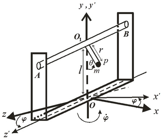
The aim of this section is to derive the equation of motion of a simple pendulum of an arm $r$ fixed from one end in a rotating axis represented by a rigid rod and the other end is attached with a mass $m$. To visualize the motion, we consider two Cartesian systems of coordinates in which the first one $Oxyz$ is fixed in space and the other $O{x}^{\prime }{y}^{\prime }{z}^{\prime }$ is fixed in the body and rotates with it, see Figure 1. The rod is connected with a rotating rigid frame with constant angular velocity $\mathsf{\Omega }=\dot{\phi }$ about the vertical axes $Oy$ and $O{y}^{\prime }$. Here, $\phi$ is the angle of rotation of the rotary frame $Oxyz$ about the vertical axis $Oy$.

Figure 1. The dynamical model.

Therefore, we can write

$$\begin{array}{l}z=z^{\prime }\cos \phi -x^{\prime }\sin \phi ,\\ x=x^{\prime }\cos \phi +z^{\prime }\sin \phi ,\end{array}$$

(1)

where

$$\begin{array}{l}{x}^{\prime }=r\sin \theta ,\\ y^{\prime }=y=l-r\cos \theta ,\\ z^{\prime }=0,\end{array}$$

(2)

where $\theta$ is the angle of inclination of the T-shaped with the vertical axis and $l$ is the distance from the rotating axis (rigid rod) of the pendulum to $z$-axis. Based on the above, one obtains easily

$$\begin{array}{l}x=r\sin \theta \cos \phi ,\\ y=l-r\cos \theta ,\\ z=-r\sin \theta \sin \phi .\end{array}$$

(3)

Making use of the above projections of the point $p$ on the coordinates system $Oxyz$ to write the kinetic and the potential energies in the form

$$\begin{array}{l}T=\frac{1}{2}m{r}^2({\dot{\theta }}^2+{\mathsf{\Omega }}^2{\sin }^2\theta ),\\ V=mg(l-r\cos \theta ),\end{array}$$

(4)

where dots denote the derivative with respect to time $t$ and $g$ is the gravitational acceleration.

According to the variational theory [36,37,38], the Lagrange’s equation for conservative dynamical systems is

$$\frac{d}{dt}(\frac{\partial L}{\partial \dot{\theta }})-\frac{\partial L}{\partial \theta }=0,$$

(5)

where $L=T-V$ is the Lagrangian, the equation of motion (EOM) has therefore the form

$$\frac{r}{g}\ddot{\theta }+(1-\Lambda \cos \theta )\sin \theta =0,$$

(6)

where $\Lambda ={\mathsf{\Omega }}^{2}r/g$.

Now, let us introduce a new independent variable $\tau$ in the form

$$\tau =\sqrt{\frac{g}{r}}t.$$

(7)

According to (7), we can rewrite the EOM (6) in the form

$${\theta }^{″}+(1-\Lambda \cos \theta )\sin \theta =0,$$

(8)

where prims denote the derivative with respect to time $\tau$.

3. The Homotopy Perturbation Method

In this section, we outline on the HPM through consideration of the following nonlinear equation

$$K(\theta )-f(r)=0,\hspace{1em}\hspace{1em}\hspace{1em}r\in {\mathsf{\Omega }}^{*},$$

(9)

with the boundary condition

$$B(\theta ,\frac{\partial \theta }{\partial n})=0,\hspace{1em}\hspace{1em}\hspace{1em}r\in \Gamma .$$

(10)

Here $K,B,f$ and $\Gamma$ are a general differential operator, a boundary one, analytical function, and the boundary of a domain ${\mathsf{\Omega }}^{*}$. Moreover, $\frac{\partial \theta }{\partial n}$ represent the differential along the normal drawn outwards from ${\mathsf{\Omega }}^{*}$.

According to HPM, we can separate the operator $K$ into linear and nonlinear parts $L$ and $N$ respectively. Consequently, one can rewrite Equation (9) in the form

$$L(\theta )+N(\theta )-f(r)=0$$

(11)

An inspection of Equation (10) shows that we can formulate a homotopy of (10) to satisfy $\theta (r,\rho ):{\mathsf{\Omega }}^{*}\times [0,1]\to R$,

$$H(\theta ,\rho )=L(\theta )-L(U)+\rho L(U)+\rho [N(\theta )-f(r)]=0,\hspace{1em}\hspace{1em}\rho \in [0,1]$$

(12)

where $\rho$ is an embedding parameter and $U$ is an initial approximation guess of Equation (9), in which the boundary conditions are fulfilled.

Based on the HPM, the solution of (12) can be expanded into a power series of $\rho$ as

$$\theta ={\theta }_0+\rho {\theta }_1+{\rho }^2{\theta }_2+\dots .$$

(13)

When $\rho \to 1$, will find that Equation (12) matches with Equation (9) and therefore, we can express the asymptotic solution of Equation (9) in the form

$$v=\underset{\rho \to 1}{\lim }\theta ={\theta }_0+{\theta }_1+{\theta }_2+\dots .$$

(14)

It is noteworthy that, in many cases, the series (14) is convergent. For the convergence of this sequence, some certain conditions are proposed [7].

4. Method of Solution

The purpose of this section is to employ the HPM to obtain the asymptotic solution of the EOM. Substituting the following expansion of the trigonometric function $\sin \theta$ into the EOM (8)

$$\sin \theta =\theta -\frac{{\theta }^3}{3!}+\dots ,$$

(15)

to get its approximation form

$${\theta }^{″}+(1-\Lambda )\theta +(\frac{4\Lambda -1}{3!}){\theta }^3+\dots =0.$$

(16)

Let’s consider the initial conditions of the above equation in the form

$$\theta (0)=1,\hspace{1em}\hspace{1em}{\theta }^{\prime }(0)=0.$$

(17)

According to (11), we can express the linear and nonlinear parts $L(\theta )$ and $N(\theta )$ of Equation (16) as follows

$$L(\theta )={\theta }^{″}+(1-\Lambda )\theta ,$$

(18)

$$N(\theta )=(\frac{4\Lambda -1}{3!}){\theta }^3,$$

(19)

where

$$f(t)=0.$$

(20)

It is possible to rewrite Equation (12) in the form

$$H(\theta ,\rho )=(1-\rho )[L(\theta )-L(U)]+\rho [L(\theta )+N(\theta )-f(t)]=0,\hspace{1em}\rho \in [0,1]$$

(21)

The substituting of (18)–(20) into (21) yields

$$\begin{array}{l}H(\theta ,\rho )=(1-\rho )[{\theta }^{″}+(1-\Lambda )\theta -U^{″}-(1-\Lambda )U]\\ \hspace{1em}\hspace{1em}\hspace{1em}+\rho [{\theta }^{″}+(1-\Lambda )\theta +(\frac{4\Lambda -1}{3!}){\theta }^3]=0,\end{array}$$

(22)

where $U$ is the initial approximation guess. It does not depend on the boundary conditions. So that we may choose a specific value or function to make the solution easier and shorter.

For simplicity we set $U=0$, Equation (22) has the following form

$$H(\theta ,\rho )={\theta }^{″}+(1-\Lambda )\theta +\rho (\frac{4\Lambda -1}{3!}){\theta }^3=0.$$

(23)

Substituting the power series (13) into (23), and equating the coefficients of different powers of $\rho$ with zero, we get

Coefficients of ${\rho }^0$:

$${{\theta }^{″}}_0+(1-\Lambda ){\theta }_0=0.$$

(24)

Coefficients of ${\rho }^1$:

$${\theta }_1{}^{″}+(1-\Lambda ){\theta }_1+(\frac{4\Lambda -1}{6}){\theta }_0{}^3=0.$$

(25)

Coefficients of ${\rho }^{{}^2}$:

$${\theta }_2{}^{″}+(1-\Lambda ){\theta }_2+(\frac{4\Lambda -1}{2}){\theta }_1{\theta }_0{}^2=0.$$

(26)

The inspection of the above Equations (24)–(26) shows that we can solve them sequentially with the use of the following initial conditions

$$\begin{array}{l}{\theta }_0(0)=1,\hspace{1em}\hspace{1em}\hspace{1em}{{\theta }^{\prime }}_0(0)=0,\\ {\theta }_1(0)=0,\hspace{1em}\hspace{1em}\hspace{1em}{{\theta }^{\prime }}_1(0)=0,\\ {\theta }_2(0)=0,\hspace{1em}\hspace{1em}\hspace{1em}{{\theta }^{\prime }}_2(0)=0,\end{array}$$

(27)

to obtain

$${\theta }_0=\cos (\tau \sqrt{1-\Lambda }),$$

(28)

$${\theta }_1=\frac{[4(1-\Lambda )-3]}{96(1-\Lambda )}[6\sqrt{1-\Lambda }\tau +\sin (2\sqrt{1-\Lambda }\tau )]\sin (\sqrt{1-\Lambda }\tau ),$$

(29)

$$\begin{array}{l}{\theta }_2=-\frac{{[3-4(1-\Lambda )]}^2}{36864{(1-\Lambda )}^2}\{[72(1-\Lambda ){\tau }^2-23]\cos (\sqrt{1-\Lambda }\tau )+24\cos (3\sqrt{1-\Lambda }\tau )\\ \hspace{1em}\hspace{1em}-\cos (5\sqrt{1-\Lambda }\tau )+12\tau \sqrt{1-\Lambda }[3\sin (3\sqrt{1-\Lambda }\tau )-8\sin (\sqrt{1-\Lambda }\tau )]\}\end{array}$$

(30)

Substituting (28)–(30) into (13) to obtain

$$\begin{array}{l}\theta =\cos (\sqrt{1-\Lambda }\tau )+\rho [\frac{[4(1-\Lambda )-3]}{96(1-\Lambda )}[6\sqrt{1-\Lambda }\tau +\sin (2\sqrt{1-\Lambda }\tau )]\sin (\sqrt{1-\Lambda }\tau )]\\ \hspace{1em}+{\rho }^2\{-\frac{{[3-4(1-\Lambda )]}^2}{36864{(1-\Lambda )}^2}\{[72{\tau }^2(1-\Lambda )-23]\cos (\sqrt{1-\Lambda }\tau )+24\cos (3\sqrt{1-\Lambda }\tau )\\ \hspace{1em}-\cos (5\sqrt{1-\Lambda }\tau )+12\tau \sqrt{1-\Lambda }[3\sin (3\sqrt{1-\Lambda }\tau )-8\sin (\sqrt{1-\Lambda }\tau )]\left\}\right\}.\end{array}$$

(31)

According to (14), the above approximate solution has the form

$$\begin{array}{l}v=\underset{\rho \to 1}{\lim }\theta =\cos (\sqrt{1-\Lambda }\tau )+\frac{[4(1-\Lambda )-3]}{96(1-\Lambda )}[6\sqrt{1-\Lambda }\tau +\sin (2\sqrt{1-\Lambda }\tau )]\sin (\sqrt{1-\Lambda }\tau )\\ \hspace{1em}-\frac{{[3-4(1-\Lambda )]}^2}{36864{(1-\Lambda )}^2}\{[72{\tau }^2(1-\Lambda )-23]\cos (\sqrt{1-\Lambda }\tau )+24\cos (3\sqrt{1-\Lambda }\tau )\\ \hspace{1em}-\cos (5\sqrt{1-\Lambda }\tau )+12\tau \sqrt{1-\Lambda }[3\sin (3\sqrt{1-\Lambda }\tau )-8\sin (\sqrt{1-\Lambda }\tau )\}].\end{array}$$

(32)

Numerically, the successive approximations by the HPM (with a finite series) are guaranteed to converge to the exact solution over some intervals. Therefore, $v(\tau )$ converges locally uniform.

5. Stability Analysis

The main objective of this section is to study the stability of the considered dynamical model by examining its EOM (16), in which it isn’t useful to study stability through the obtained solution (32). Therefore, we are going to consider the linear and nonlinear parts of Equation (16) in which they are represented by Equations (18) and (19) respectively. It is worthy to mention that, the stability of the linear part depends on the frequency term $(1-\Lambda )$ which is always positive. Therefore, this term can be expanded in a power series of $\rho$ as follows

$$(1-\Lambda )={\omega }^2+\rho {\omega }_1+{\rho }^2{\omega }_2+\dots$$

(33)

Substituting from Equation (13) about $\theta$ and from (33) about the expanded frequency into Equation (16) and equating the coefficients of equal powers of $\rho$ for both sides of the resulted equation to get

Coefficient of ${\rho }^0$:

$${{\theta }^{″}}_0+{\omega }^2{\theta }_0=0,$$

(34)

Coefficient of $\rho$:

$${\theta }_1{}^{″}+{\omega }^2{\theta }_1+{\omega }_1{\theta }_0+\frac{1}{6}(4\Lambda -1){\theta }_0{}^3=0,$$

(35)

Taking into account the previous initial conditions (27), we can write the solution of the homogenous Equation (34) in the form

$${\theta }_0=\cos (\tau \omega ).$$

(36)

Therefore Equation (35) becomes

$${\theta }_1{}^{″}+{\omega }^2{\theta }_1=-{\omega }_1\cos (\tau \omega )-\frac{1}{6}(4\Lambda -1){\cos }^3(\tau \omega ).$$

(37)

Elimination of the secular terms demands that

$${\omega }_1=-\frac{1}{8}(4\Lambda -1).$$

(38)

Considering the initial conditions ${\theta }_1(0)={{\theta }^{\prime }}_1(0)=0$, we can write the solution of (37) after elimination of the secular term in the form

$${\theta }_1=\frac{(4\Lambda -1)}{24(7-4\Lambda )}[\cos (3\tau \omega )-\cos (\tau \omega )].$$

(39)

Making use of (38) into (33) and considering $\rho =1$, one can write the obtained frequency in the form

$${\omega }^2=\frac{1}{8}(7-4\Lambda ).$$

(40)

In order to keep the system stable, we must consider the following stability condition

$$\Lambda <\frac{7}{4}.$$

(41)

6. He’s Frequency Formulation

In order to verify our above results, this section introduces briefly He’s frequency formulation [38,39]. Considering a nonlinear oscillator in the form

$${\theta }^{″}+g(\theta )=0$$

(42)

with initial conditions

$$\theta (0)=A,{\theta }^{\prime }(0)=0$$

(43)

where g is a smooth function. Equation (42) has periodic solution when

$$\frac{d^2}{d{\theta }^2}g(\theta )>0$$

(44)

He’s frequency formulation is [38,39]

$${\omega }^2={\frac{d}{d\theta }g(\theta )|}_{\theta =A/2}$$

(45)

In our study,

$$g(\theta )=(1-\Lambda )\theta +(\frac{4\Lambda -1}{3!}){\theta }^3$$

(46)

It is easy to find that

$$\frac{d}{d\theta }g(\theta )=1-\Lambda +(\frac{4\Lambda -1}{2}){\theta }^2$$

(47)

In our study A = 1, according to Equation (45), we obtain

$${\omega }^2=1-\Lambda +\frac{4\Lambda -1}{8}=\frac{7-4\Lambda }{8}$$

(48)

This is exactly same as that given in Equation (40). Applications of He’s frequency formulation are referred to refs [40,41,42,43,44,45].

7. Results and Discussion

This section sheds light on the great accuracy of the obtained results that are achieved by using HPM through the comparison of these results with the numerical ones that are gained by utilizing the fourth-order RKM [46,47,48].

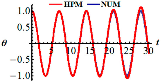
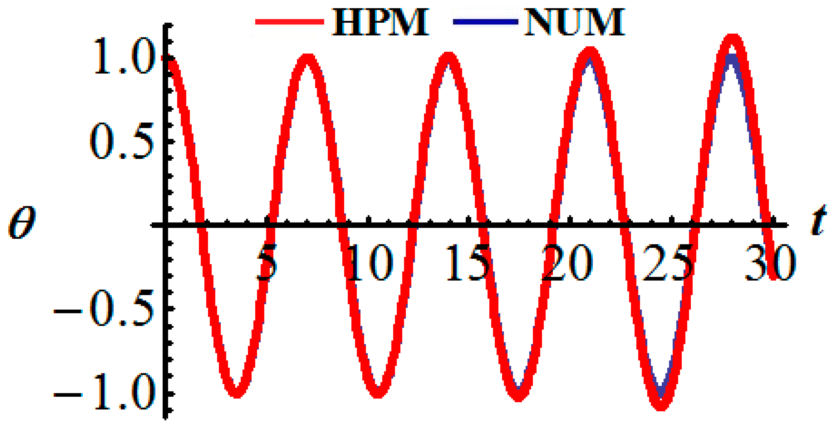
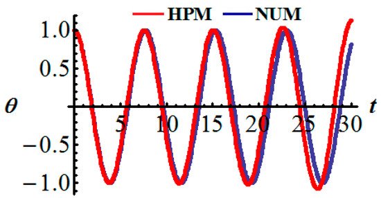
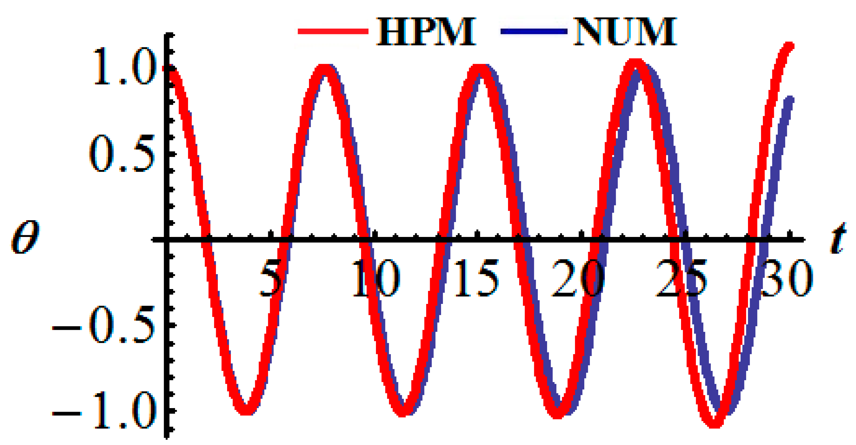
A beneficial way for a good comparison between the attained asymptotic results by HPM and the numerical ones obtained by RKM, is to look reviews them through the Table 1, Table 2, Table 3, Table 4, Table 5 and Table 6 in addition to the error between them. The results included in Table 1, Table 2, Table 3, Table 4, Table 5 and Table 6 correspond to the curves of Figure 2, Figure 3, Figure 4, Figure 5, Figure 6 and Figure 7 respectively for the same corresponding values of $r$ and $\mathsf{\Omega }$.

Table 1. Error percentage of HPM for $r=0.6\mathrm{m},\mathsf{\Omega }=1.5\mathrm{rad}{·\mathrm{s}}^{-1}$.

Time	Numerical Results (NR)	HPM Results (HPMR)	$\left|\frac{\mathit{H}\mathit{P}\mathit{M}\mathit{R}-\mathit{N}\mathit{R}}{\mathit{N}\mathit{R}}\right|$
0	1	1	0
1	0.630869	0.627776	0.0049026
2	0.21956	−0.225384	0.0265278
3	−0.899482	−0.903169	0.00409939
4	−0.908171	−0.903095	0.00558896
5	−0.239734	−0.22469	0.0627527
6	0.614791	0.628734	0.02268
7	0.999796	1.00071	0.000911276
8	0.646672	0.630153	0.0255458
9	−0.199286	−0.225065	0.129353
10	−0.890417	−0.903541	0.0147397

Table 2. Error percentage of HPM for r = 0.6 m, Ω = 2 rad s⁻¹.

Time	Numerical Results (NR)	HPM Results (HPMR)	$\left|\frac{\mathit{H}\mathit{P}\mathit{M}\mathit{R}-\mathit{N}\mathit{R}}{\mathit{N}\mathit{R}}\right|$
0	1	1	0
1	0.654764	0.64695	0.0119336
2	−0.148467	−0.16355	0.101592
3	−0.847042	−0.858298	0.013288
4	−0.956805	−0.946617	0.0106482
5	−0.404543	−0.366363	0.0943759
6	0.432158	0.473118	0.0947819
7	0.965135	0.977907	0.0132337
8	0.830583	0.792124	0.046304
9	0.118301	0.0465204	0.606763
10	−0.677385	−0.73201	0.0806414

Table 3. Error percentage of HPM for r = 0.6 m, Ω = 2.5 rad s⁻¹.

Time	Numerical Results (NR)	HPM Results (HPMR)	$\left|\frac{\mathit{H}\mathit{P}\mathit{M}\mathit{R}-\mathit{N}\mathit{R}}{\mathit{N}\mathit{R}}\right|$
0	1	1	0
1	0.685404	0.671387	0.0204506
2	0.0527615	−0.0808787	0.532912
3	−0.758994	0.783883	0.0327925
4	−0.99427	−0.985533	0.00878713
5	−0.604164	0.538474	0.108728
6	0.157724	0.242582	0.538009
7	0.824048	0.875886	0.0629072
8	0.977147	0.942131	0.0358349
9	0.51624	0.385223	0.253791
10	−0.261008	−0.404121	0.548309

Table 4. Error percentage of HPM for r = 0.3 m, Ω = 2 rad s⁻¹.

Time	Numerical Results (NR)	HPM Results (HPMR)	$\left|\frac{\mathit{H}\mathit{P}\mathit{M}\mathit{R}-\mathit{N}\mathit{R}}{\mathit{N}\mathit{R}}\right|$
0	1	1	0
1	0.627452	0.625023	0.00387119
2	−0.229458	−0.23406	0.0200579
3	−0.905921	−0.908752	0.00312526
4	0.900042	−0.896209	0.00425873
5	0.215822	−0.204251	0.0536163
6	0.638176	0.648882	0.0167751
7	0.999907	1.00072	0.000812474
8	0.616603	0.605241	0.0184257
9	−0.243047	0.262363	0.0794747
10	0.911628	−0.921237	0.0105405

Table 5. Error percentage of HPM for r = 0.9 m, Ω = 2 rad s⁻¹.

Time	Numerical Results (NR)	HPM Results (HPMR)	$\left|\frac{\mathit{H}\mathit{P}\mathit{M}\mathit{R}-\mathit{N}\mathit{R}}{\mathit{N}\mathit{R}}\right|$
0	1	1	0
1	0.682004	0.668681	0.0195354
2	−0.0636153	−0.0902769	0.419106
3	0.770003	0.793214	0.0301438
4	0.991721	0.982383	0.0094154
5	−0.582943	0.520499	0.107117
6	0.189856	0.269191	0.417868
7	0.845418	0.891707	0.0547537
8	0.967025	0.929664	0.038635
9	0.474508	0.35122	0.259822
10	−0.313132	−0.443194	0.415355

Table 6. Error percentage of HPM for r = 1.1 m, Ω = 2 rad s⁻¹.

Time	Numerical Results (NR)	HPM Results (HPMR)	$\left|\frac{\mathit{H}\mathit{P}\mathit{M}\mathit{R}-\mathit{N}\mathit{R}}{\mathit{N}\mathit{R}}\right|$
0	1	1	0
1	0.700116	0.68309	0.0243185
2	−0.00515091	−0.0393558	6.64055
3	−0.707562	−0.739703	0.0454255
4	−0.999944	0.995252	0.00469164
5	−0.692595	0.611115	0.117644
6	0.0154523	0.129692	7.39304
7	0.714933	0.793976	0.11056
8	0.999775	0.983871	0.0159081
9	0.685001	0.518703	0.24277
10	−0.0257521	−0.252657	8.81111

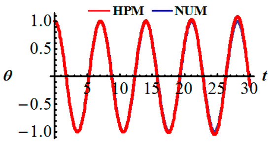
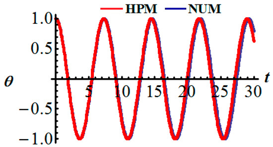
Figure 2. Illustrates the time history of the approximate solutions (red color) and numerical solution (blue color) at $r=0.6$ and $\mathsf{\Omega }=1.5$.

Figure 3. Shows the time history of the approximate solutions (red color) and numerical solution (blue color) at $r=0.6$ and $\mathsf{\Omega }=2$.

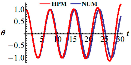
Figure 4. Reveals a comparison between the analytical solution obtained by HPM (red color) and the numerical one obtained by RKM (blue color) $r=0.6$ and $\mathsf{\Omega }=2.5$.

Figure 5. Shows a comparison between the time histories of the approximate solution (red color) and the numerical one (blue color) $\mathsf{\Omega }=2$ and $r=0.3$.

Figure 6. Portrays the comparison between the analytic solution (red color) and the numerical one (blue color) $\mathsf{\Omega }=2$ and $r=0.9$.

Figure 7. Shows a comparison between the homotopy solution (red color) and the numerical one (blue color) $\mathsf{\Omega }=2$ and $r=1.1$.

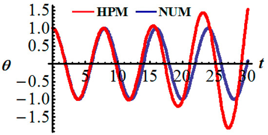
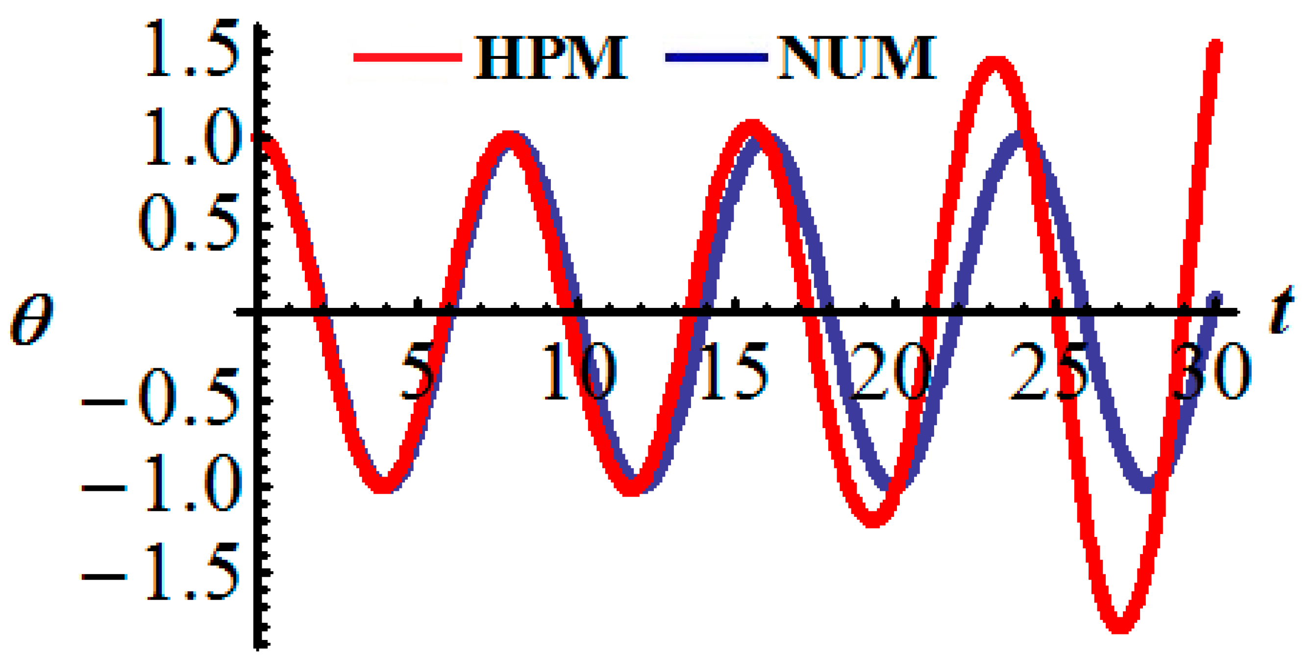
The curves displayed Figure 2, Figure 3 and Figure 4 are calculated when r = 0.6 m with the distinct values of $\mathsf{\Omega }=(1.5,2,2.5)\mathrm{rad}·{\mathrm{s}}^{-1}$ while Figure 6 and Figure 7 are plotted when $\mathsf{\Omega }=2$ at $r=0.6$. The objective of these curves is to reveal the comparison between the approximate analytical solutions that are represented in Equation (32) (with red color) and the numerical solutions of the governing EOM (8) (with blue color). These drawings indicate that the comparison between both results reaches a peak of congruence at $r=0.6$ when $\mathsf{\Omega }=1.5$ and $\mathsf{\Omega }=2$ as seen in Figure 2 and Figure 3 respectively. On the other side, this comparison is not completely consistent when $r=0.6$ and $\mathsf{\Omega }=2.5$ for the attained solutions after the elapse of half period time, as shown in Figure 4. A closer look at these figures shows that the plotted curves have aperiodic behavior, which confirms the stability of the obtained solutions.

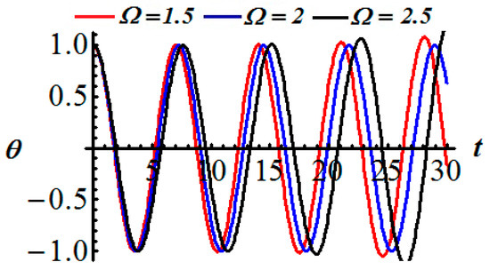
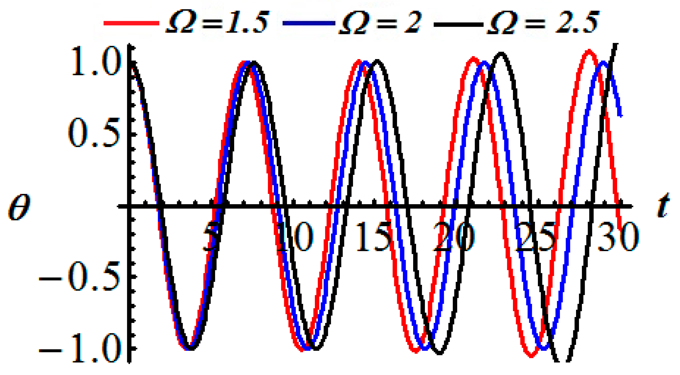
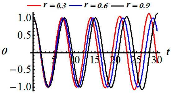
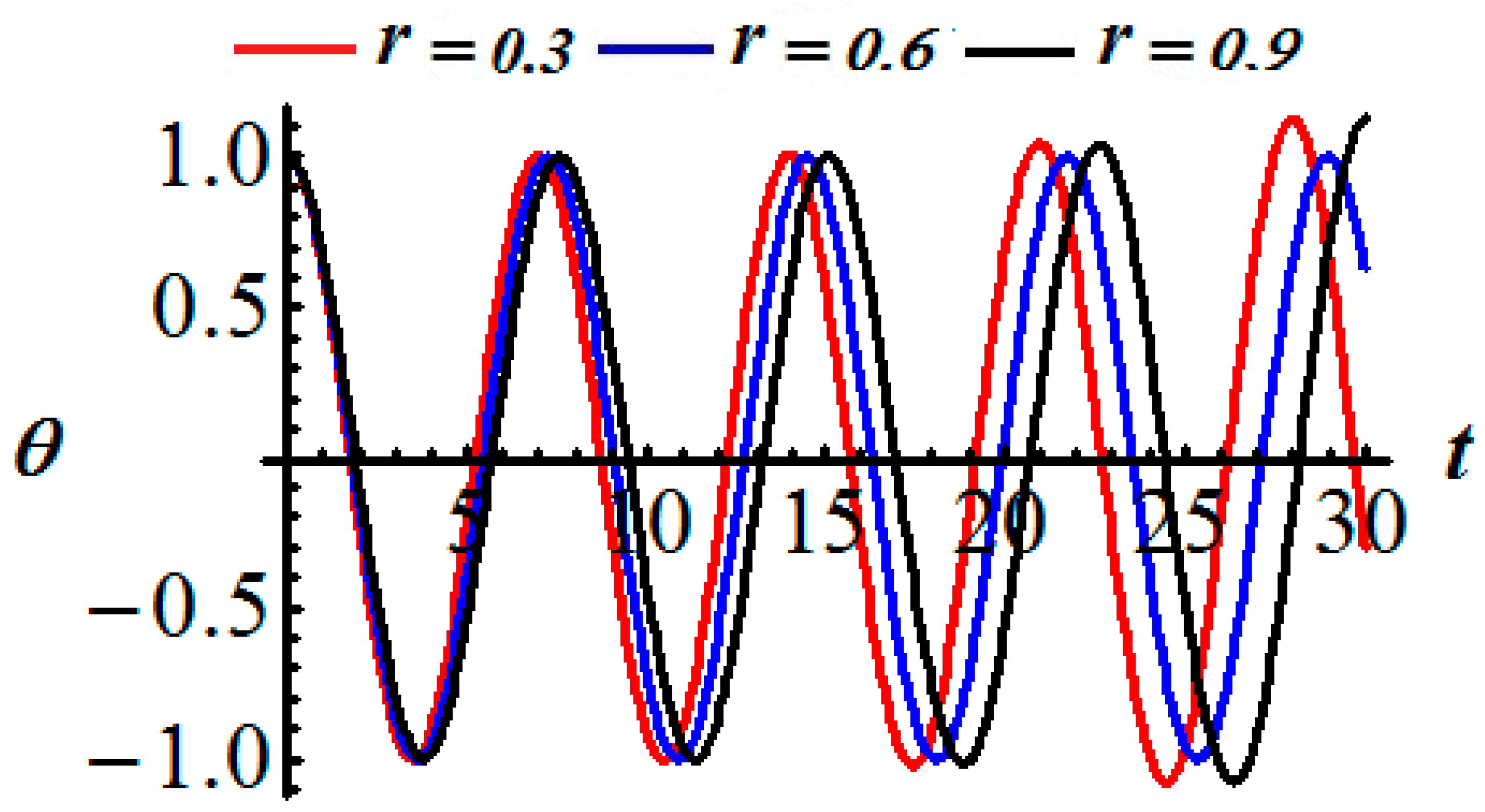
The purpose of the graphically generated results Figure 8 and Figure 9 is to investigate the impact of different values of $\mathsf{\Omega }=(1.2,2,2.5)\mathrm{rad}{·\mathrm{s}}^{-1}$ and $r(=0.3,0.6,0.9)\mathrm{m}$ respectively, with the constancy of $r=0.6$ in Figure 8 and $\mathsf{\Omega }=2$ in Figure 9 on the behavior of the considered dynamical model. It is clear that when $\mathsf{\Omega }$ and $r$ increase, the amplitudes of the waves increase to some extent besides the constancy of the oscillations number and wavelengths.

Figure 8. Describes the impact of distinct values of $\mathsf{\Omega }(=1.5,2,2.5)$ on the solution $\theta$ at $r=0.6$.

Figure 9. Explores the effect of the different values of $r(=0.3,0.6,0.9)$ on the solution $\theta$ at $\mathsf{\Omega }=2$.

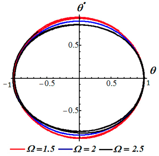
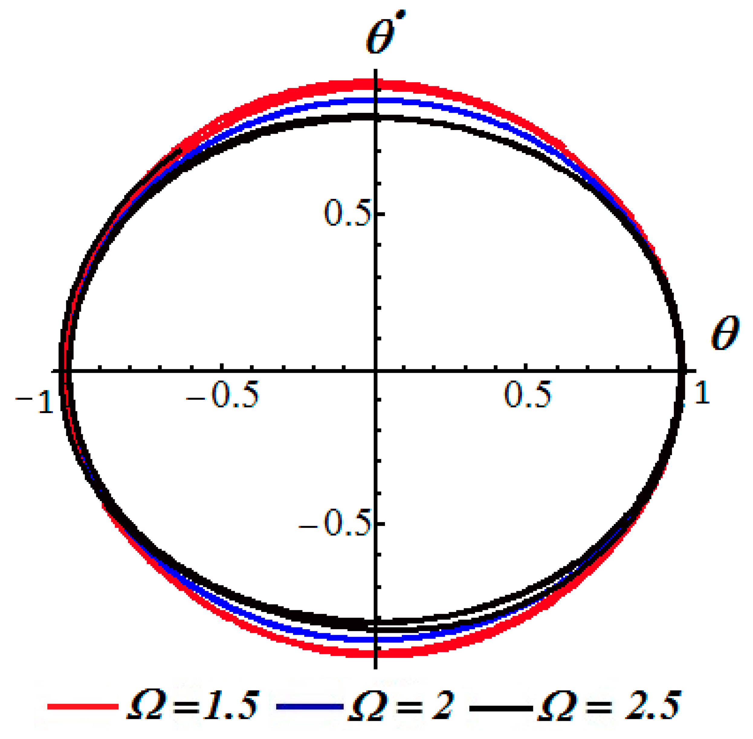
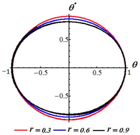
The phase plane diagrams that assert the stability of the attained solution, at different values of $\mathsf{\Omega }$ and $r$, are represented graphically in Figure 10 and Figure 11 respectively.

Figure 10. Describes the phase plane of the solution at $\mathsf{\Omega }(=1.5,2,2.5)$ when $r=0.6$.

Figure 11. Describes the phase plane of the solution at $r(=0.3,0.6,0.9)$ when $\mathsf{\Omega }=2$.

8. Conclusions

The asymptotic periodic solution of the EOM of a simple pendulum fixed in a rotating rigid frame is obtained using HPM. The numerical solution of the governing EOM is achieved utilizing the fourth-order RKM. A comparison between the attained solutions, whether analytical or numerical, showed a clear match between them which emphasizes the accuracy of the used HPM. These solutions are performed through computer codes to represent the time histories of the motion graphically at the distinct values of the physical parameters of the studied model. The stability condition of the motion is obtained.

References

- Ji, W.M.; Wang, H.; Liu, M. Dynamics analysis of an impulsive stochastic model for spruce budworm growth. Appl. Comput. Math. 2021, 19, 336–359. [Google Scholar]
- Janevski, G.; Kozic, P.; Pavlovic, R.; Posavljak, S. Moment Lyapunov exponents and stochastic stability of a thin-walled beam subjected to axial loads and end moments. Facta Univ. Ser. Mech. Eng. 2021, 19, 209–228. [Google Scholar] [CrossRef] [Scilit]
- Pavlovic, I.R.; Pavlovic, R.; Janevski, G.; Despenić, N.; Pajković, V. Dynamic behavior of two elastically connected nanobeams under a white noise process. Facta Univ. Ser. Mech. Eng. 2020, 18, 219–227. [Google Scholar] [CrossRef] [Scilit]
- Zuo, Y.-T. A gecko-like fractal receptor of a three-dimensional printing technology: A fractal oscillator. J. Math. Chem. 2021, 59, 735–744. [Google Scholar] [CrossRef] [Scilit]
- Yeasmin, I.A.; Rahman, M.S.; Alam, M.S. The modified Lindstedt-Poincare method for solving quadratic nonlinear oscillators. J. Low Freq. Noise Vib. Act. Control 2020, 1461348420979758. [Google Scholar] [CrossRef] [Scilit]
- El-Sabaa, F.M.; Amer, T.S.; Gad, H.M.; Bek, M.A. On the motion of a damped rigid body near resonances under the influence of harmonically external force and moments. Results Phys. 2020, 19, 103352. [Google Scholar] [CrossRef] [Scilit]
- He, J.H. Homotopy perturbation technique. Comput. Meth. Appl. Mech. Eng. 1999, 178, 257–262. [Google Scholar] [CrossRef] [Scilit]
- Anjum, N.; Ain, Q.T. Application of He’s fractional derivative and fractional complex transform for time fractional Camassa-Holm equation. Therm. Sci. 2020, 24, 3023–3030. [Google Scholar] [CrossRef] [Scilit]
- El-Dib, Y.O. Homotopy perturbation for excited nonlinear equations. Sci. Eng. Appl. 2017, 2, 96–108. [Google Scholar] [CrossRef] [Scilit]
- Amer, T.S.; Galal, A.A.; Elnaggar, S. The vibrational motion of a dynamical system using homotopy perturbation technique. Appl. Math. 2020, 11, 1081–1099. [Google Scholar] [CrossRef]
- El-Dib, Y.O.; Moatimid, G.M. Stability configuration of a rocking rigid rod over a circular surface using the homotopy perturbation method and Laplace transform. Arab. J. Sci. Eng. 2019, 44, 6581–6591. [Google Scholar] [CrossRef] [Scilit]
- Ganji, S.S.; Ganji, D.D.; Babazadeh, H.; Karimpour, S. Variational approach method for nonlinear oscillations of the motion of a rigid rocking back and forth and cubic-quintic Duffing oscillators. Prog. Electromagn. Res. M 2008, 4, 23–32. [Google Scholar] [CrossRef] [Scilit]
- El-Dib, Y.O. Periodic solution and stability behavior for nonlinear oscillator having a cubic nonlinearity time-delayed. Int. Annu. Sci. 2018, 5, 12–25. [Google Scholar] [CrossRef] [Scilit]
- El-Dib, Y.O. Periodic solution of the cubic nonlinear Klein-Gordon equation and the stability criteria via the He-multiple-scales method. Pramana J. Phys. 2019, 92, 7. [Google Scholar] [CrossRef] [Scilit]
- El-Dib, Y.O. Stability approach for periodic delay Mathieu equation by the He-multiple-scales method. Alex. Eng. J. 2018, 57, 4009–4020. [Google Scholar] [CrossRef] [Scilit]
- Hosen, M.A.; Chowdhury, M.S.H. Accurate approximations of the nonlinear vibration of couple-mass-springs systems with linear and nonlinear stiffnesses. J. Low Freq. Noise Vib. Act. Control 2021, 40, 1072–1090. [Google Scholar] [CrossRef] [Scilit]
- Hosen, M.A. Analysis of nonlinear vibration of couple-mass–spring systems using iteration technique. Multidiscip. Modeling Mater. Struct. 2020, 16, 1539–1558. [Google Scholar] [CrossRef] [Scilit]
- Anjum, N.; He, J.H. Homotopy perturbation method for N/MEMS oscillators. Math. Methods Appl. Sci. 2020. [Google Scholar] [CrossRef] [Scilit]
- Tian, D.; Ain, Q.-T.; Anjum, N.; He, C.-H.; Cheng, B. Fractal N/MEMS: From pull-in instability to pull-in stability. Fractals 2021, 29, 2150030. [Google Scholar] [CrossRef] [Scilit]
- Meshki, H.; Rezaei, A.; Sadeghi, A. Homotopy Perturbation-Based Dynamic Analysis of Structural Systems. J. Eng. Mech. 2020, 146, 04020136. [Google Scholar] [CrossRef] [Scilit]
- Wang, K.L.; Yao, S.W. He’s fractiona; derivative for the evolution equation. Therm. Sci. 2020, 24, 2507–2513. [Google Scholar] [CrossRef] [Scilit]
- He, J.H.; El-Dib, Y.O. The enhanced homotopy perturbation method for axial vibration of strings. Facta Univ. Ser. Mech. Eng. 2021. [Google Scholar] [CrossRef] [Scilit]
- He, C.H.; Tian, D.; Moatimid, G.M.; Salman, H.F.; Zekry, M.H. Hybrid Rayleigh-Van der Pol-Duffing Oscillator (HRVD): Stability Analysis and Controller. J. Low Freq. Noise Vib. Act. Control 2021. [Google Scholar] [CrossRef] [Scilit]
- He, J.-H.; Galal, M.M.; Mostapha, D.R. Nonlinear Instability of Two Streaming-Superposed Magnetic Reiner-Rivlin Fluids by He-Laplace Method. J. Electroanal. Chem. 2021, 895, 115388. [Google Scholar] [CrossRef] [Scilit]
- Anjum, N.; He, J.H.; Ain, Q.T.; Tian, D. Li-He’s modified homotopy perturbation method for doubly-clamped electrically actuated microbeams-based microelectromechanical system. Facta Univ. Ser. Mech. Eng. 2021. [Google Scholar] [CrossRef] [Scilit]
- El-Dib, Y.O.; Matoog, R.T. The Rank Upgrading Technique for a Harmonic Restoring Force of Nonlinear Oscillators. J. Appl. Comput. Mech. 2021, 7, 782–789. [Google Scholar] [CrossRef] [Scilit]
- Elgazery, N.S. A Periodic Solution of the Newell-Whitehead-Segel (NWS) Wave Equation via Fractional Calculus. J. Appl. Comput. Mech. 2020, 6, 1293–1300. [Google Scholar]
- Koochi, A.; Goharimanesh, M. Nonlinear Oscillations of CNT Nano-resonator Based on Nonlocal Elasticity: The Energy Balance Method. Rep. Mech. Eng. 2021, 2, 41–50. [Google Scholar] [CrossRef] [Scilit]
- Filobello-Nino, U.; Vazquez-Leal, H.; Herrera-May, A.; Ambrosio, R.; Jimenez-Fernandez, V.M.; Sandoval-Hernandez, M.A.; Alvarez-Gasca, O.; Palma-Grayeb, B.E. The study of heat transfer phenomena by using modified homotopy perturbation method coupled by Laplace transform. Therm. Sci. 2020, 24, 1105–1115. [Google Scholar] [CrossRef] [Scilit]
- Li, X.X.; He, C.H. Homotopy perturbation method coupled with the enhanced perturbation method. J. Low Freq. Noise Vib. Act. Control 2019, 38, 1399–1403. [Google Scholar] [CrossRef] [Scilit]
- Mahmudov, N.I.; Huseynov, I.T.; Aliev, N.A.; Aliev, F.A. Analytical approach to a class of Bagley-Torvik equations. TWMS J. Pure Appl. Math. 2020, 11, 238–258. [Google Scholar]
- Qalandarov, A.A.; Khaldjigitov, A.A. Mathematical and Numerical modeling of the coupled dynamic thermoelastic problems for isotropic bodies. TWMS J. Pure Appl. Math. 2020, 11, 119–126. [Google Scholar]
- Fikret, A.A.; Aliev, N.A.; Mutallimov, M.M.; Namazov, A.A. Algorithm for solving the identification problem for determining the fractional-order derivative of an oscillatory system. Appl. Comput. Math. 2020, 19, 435–442. [Google Scholar]
- Zhang, J.J.; Shen, Y.; He, J.H. Some analytical methods for singular boundary value problem in a fractal space: A review. Appl. Comput. Math. 2019, 18, 225–235. [Google Scholar]
- Song, H.Y. A thermodynamic model for a packing dynamic system. Therm. Sci. 2020, 24, 2331–2335. [Google Scholar] [CrossRef] [Scilit]
- Yao, S.W. Variational principle for non-linear fractional wave equation in a fractal space. Therm. Sci. 2021, 25, 1243–1247. [Google Scholar] [CrossRef] [Scilit]
- Liu, H.Y.; Li, Z.M.; Yao, S.W.; Yao, Y.J.; Liu, J. A variational principle for the photocatalytic Nox abatement. Therm. Sci. 2020, 24, 2515–2518. [Google Scholar] [CrossRef] [Scilit]
- He, J.H. The simpler, the better: Analytical methods for nonlinear oscillators and fractional oscillators. J. Low Freq. Noise Vib. Act. Control 2019, 38, 1252–1260. [Google Scholar] [CrossRef] [Scilit]
- Qie, N.; Hou, W.F.; He, J.H. The fastest insight into the large amplitude vibration of a string. Rep. Mech. Eng. 2020, 2, 1–5. [Google Scholar] [CrossRef] [Scilit]
- Liu, C.X. Periodic solution of fractal Phi-4 equation. Therm. Sci. 2021, 25, 1345–1350. [Google Scholar] [CrossRef] [Scilit]
- Liu, C.X. A short remark on He’s frequency formulation. J. Low Freq. Noise Vib. Act. Control 2021, 40, 672–674. [Google Scholar] [CrossRef] [Scilit]
- Feng, G.Q.; Niu, J.Y. He’s frequency formulation for nonlinear vibration of a porous foundation with fractal derivative. Int. J. Geomath. 2021, 12, 14. [Google Scholar] [CrossRef] [Scilit]
- Feng, G.Q. He’s frequency formula to fractal undamped Duffing equation. J. Low Freq. Noise Vib. Act. Control 2021, 1461348421992608. [Google Scholar] [CrossRef] [Scilit]
- Elías-Zúñiga, A.; Palacios-Pineda, L.M.; Jiménez-Cedeño, I.H.; Martínez-Romero, O.; Trejo, D.O. He’s frequency-amplitude formulation for nonlinear oscillators using Jacobi elliptic functions. J. Low Freq. Noise Vib. Act. Control 2020, 39, 1216–1223. [Google Scholar] [CrossRef] [Scilit]
- Wu, Y.; Liu, Y.P. Residual calculation in He’s frequency-amplitude formulation. J. Low Freq. Noise Vib. Act. Control 2021, 40, 1040–1047. [Google Scholar] [CrossRef] [Scilit]
- Gilat, A. Numerical Methods for Engineers and Scientists; Wiley: Hoboken, NJ, USA, 2013. [Google Scholar]
- Simos, T.E.; Tsitouras, C. 6th order Runge-Kutta pairs for scalar autonomous IVP. Appl. Comput. Math. 2020, 19, 412–421. [Google Scholar]
- Hussanan, A.; Khan, I.; Khan, W.A.; Chen, Z.M. Micropolar mixed convective flow Cattaneo-Christove heat flux: Non-Fourier Heat Conduction Analysis. Therm. Sci. 2020, 24, 1345–1356. [Google Scholar] [CrossRef] [Scilit]
Publisher’s Note: MDPI stays neutral with regard to jurisdictional claims in published maps and institutional affiliations. |
© 2021 by the authors. Licensee MDPI, Basel, Switzerland. This article is an open access article distributed under the terms and conditions of the Creative Commons Attribution (CC BY) license (https://creativecommons.org/licenses/by/4.0/).