


Abstract
Integrated mine–plant optimization should account for multiple geological uncertainties, yet practice typically considers only grade. Lithological domain uncertainty is a distinct source of geometallurgical variability because rock type governs comminution, recovery, cost, and blending. This paper extends a two-stage stochastic mine–plant planning framework to represent this uncertainty in a copper porphyry case study based on geological data from the Río Blanco–Los Bronces deposit in the Central Chilean Andes. Copper grade is fixed by block, while Truncated Gaussian Simulation generates realizations of tourmaline breccia and surrounding lithologies. The first stage optimizes a single long-term extraction schedule; the second evaluates recovery, processing cost at fixed throughput, Bond Work Index, and feed-composition compatibility under two adaptive operational modes. The framework combines parallelized Variable Neighborhood Descent with an embedded matheuristic for mass balance, plant capacity, and blending. Relative to a block-wise modal-domain deterministic benchmark over the same 100 validation scenarios, the stochastic plan increases mean net present value by US$2.38 million (3.28%), yielding an empirical value of the stochastic solution, and raises , , and by US$2.27, US$2.28, and US$2.53 million, respectively. These results show that lithological domain uncertainty has measurable economic value in mine–plant planning even when copper grades are fixed.
1. Introduction
Long-term mine planning is the strategic backbone of open-pit mining, as it defines the life-of-mine extraction schedule and determines how mineral resources are converted into economic value over time. Because ore deposits are only partially observed, geological uncertainty has become a central concern in strategic mine planning. Early deterministic approaches based on average geological models have progressively been complemented by stochastic optimization methods, including two-stage stochastic integer programming and simultaneous stochastic optimization, to generate plans that account for uncertain geological conditions and improve out-of-sample performance [1,2].
Within this evolution, the integration of mine planning and metallurgical plant performance has become increasingly important. The mine extraction sequence determines the quantity, timing, and characteristics of the material delivered to the plant, while plant performance determines how that material is transformed into recoverable value. Treating these components independently may lead to suboptimal decisions, since a schedule that appears attractive from a mining perspective may generate unfavorable blends, higher processing costs, or lower metallurgical recovery during processing [3,4]. Although modern approaches increasingly integrate extraction, destination, and processing decisions, the plant is often represented through fixed capacities or simplified response functions, rather than as an adaptive component whose mode allocation can respond to variable feed characteristics [2].
A large part of stochastic mine planning has focused on grade uncertainty as the main driver of supply risk [1]. However, from a geometallurgical perspective, lithological domain uncertainty represents a distinct source of variability. Lithological domains, represented in this case study by rock-type domains, are directly associated with mineralogical and textural characteristics that influence comminution behavior, Bond-Work-Index-related grinding-energy demand, blending requirements, processing cost, and metallurgical recovery [5,6]. Therefore, two blocks with the same copper grade may still have different economic and operational impacts depending on the lithological domain to which they belong. Although lithological domains are commonly used as fixed attributes to define blending requirements, plant responses, and operational modes, their spatial uncertainty is less frequently propagated explicitly through integrated mine–plant optimization models. Ignoring this uncertainty may limit the ability of the strategic plan to anticipate plant constraints and capture the value of operational flexibility.
This paper extends the two-stage stochastic mine–plant planning framework of Quelopana and Navarra [4] by explicitly incorporating lithological domain uncertainty as a categorical source of geological risk. The proposed approach keeps copper grades fixed by block and uses Truncated Gaussian Simulation (TGS) to generate alternative realizations of two lithological domains in a copper porphyry case study based on geological data from a sector of the Río Blanco–Los Bronces deposit. This design should not be interpreted as assuming that grade uncertainty is negligible; rather, it is a controlled experimental setting intended to isolate the effect of lithological domain uncertainty on integrated mine–plant planning decisions. The number of realizations used for stochastic optimization is selected through a scenario-sizing analysis based on decision stability and out-of-sample performance.
Applications of simultaneous stochastic optimization and stochastic resource-uncertainty management have shown the importance of propagating uncertainty into planning and drilling decisions rather than treating geological inputs as fixed deterministic descriptions; in these works, however, the propagated uncertainty is predominantly that of continuous grade or resource variables [7,8]. Related studies have jointly propagated rock-type and grade uncertainty in production scheduling [9], while mining-complex optimization has considered grade and material-type uncertainty together with multiple processing alternatives [10] and geometallurgical uncertainty in hardness indices within downstream processing decisions [11]. More recently, Morales and Dimitrakopoulos [12] showed that stochastic simulation of geological-domain geometries can materially affect long-term mine plans. The specific contribution of the present study is to quantify, under a controlled fixed-grade design, the economic and operational effect of uncertainty in the spatial configuration of lithological domains after propagating those domain realizations through domain-dependent plant responses within an integrated mine–plant framework.
The first-stage problem is solved using the parallelized Variable Neighborhood Descent (VND) procedure of Quelopana and Navarra [4], while the second-stage block-to-operational-mode assignment is solved using the matheuristic developed by Leiva et al. [13], which preserves mass-balance, plant-capacity, and blending-feasibility constraints. The case study compares the proposed stochastic domain-based approach with a deterministic modal-domain benchmark. This comparison is interpreted as an empirical value of the stochastic solution, using the modal-domain deterministic benchmark as a categorical analog of the expected-value solution commonly used in stochastic programming [14]. The purpose is to quantify the economic and operational value of explicitly representing lithological domain uncertainty in strategic mine–plant planning.
2. Background
2.1. Geological Domain Uncertainty
Geological domain uncertainty refers to the lack of certainty regarding the spatial arrangement and boundaries of geological domains, defined by categorical attributes such as lithology, alteration, and mineralogy [8,15,16]. This uncertainty reflects the inherent variability and potential errors in interpreting geological contacts [15,16]. In mining, inadequate characterization of these boundaries directly affects tonnage and metal content estimates, compromising project reliability and economic viability [8].
Biases in the interpretation of structural controls may invalidate the resource model and lead to unexpected reserve downgrades during mining [17]. Therefore, geologically consistent modeling requires integrating structural geometry, lithology, alteration, and mineralogy [17,18]. Current methodologies address this uncertainty through stochastic frameworks and geostatistical simulations, enabling its propagation to critical quantitative variables such as ore grade [15,19,20,21].
2.2. Value-of-Information Framing for Categorical Geological Uncertainty
In stochastic programming, the value of the stochastic solution (VSS) measures the expected performance gain obtained by using a solution that explicitly accounts for uncertainty instead of a solution derived from a deterministic expected-value problem [14]. In the classical setting, the expected-value solution is obtained by solving a deterministic problem in which the uncertain parameters are replaced by their expectations; the stochastic and expected-value solutions are then compared by evaluating both under the full uncertainty distribution. The expected value of perfect information (EVPI), in turn, represents the additional value that could be achieved if the uncertain parameters were known before the first-stage decisions were made [14].
Applying this terminology to geological domain uncertainty requires care because geological domains are categorical variables. Unlike grades or costs, geological domains cannot be meaningfully averaged block by block. Therefore, in this study, the deterministic benchmark is constructed as the block-wise modal-domain model computed from the same optimization realizations used by the stochastic plan. This modal-domain model collapses categorical uncertainty into a single deterministic geometry and is used as a categorical analog of the expected-value solution. The resulting comparison is therefore reported as an empirical value of the stochastic solution, defined relative to the modal-domain deterministic benchmark. EVPI is not computed in this work; estimating it would require scenario-specific wait-and-see schedules and is left as a future extension.
2.3. Integrated Mine-to-Plant Planning
Mine–plant integration seeks to optimize the mineral value chain as an interdependent system, where extraction, scheduling, blending, processing, and operational control decisions must be evaluated jointly. This perspective is supported by general systems theory, which states that optimizing subsystems separately does not guarantee global optimization; therefore, local improvements generate value only when the constraints and interactions of the entire mineral value chain are considered [3,22]. This view supports integrated models for evaluating technologies, plant designs, and planning strategies from a systemic mining-business perspective [2,3,10].
Strategic mine planning has evolved from block sequencing under precedence, capacity, and economic constraints toward models that incorporate processing routes, metallurgical constraints, rock types, operational modes, and downstream components. This evolution is related to the optimization of mining complexes and mineral value chains, where material can follow different processing, transportation, and transformation alternatives [2,10,23]. Thus, mine planning and metallurgical operation are interdependent decisions, since economic performance depends on both the extraction sequence and the plant’s ability to process variable ore blends [4,5,24].
Geological uncertainty is a critical source of risk because it affects resources, extraction sequencing, production targets, plant feed, and economic value. Stochastic approaches represent this uncertainty through equiprobable geological scenarios, allowing mine plans to be evaluated under different deposit realizations and enabling the construction of risk profiles [1,3,25]. In long-term planning, this variability can affect tonnage, grades, operational constraints, and economic performance [4,23].
In recent mine–plant integration approaches, geological uncertainty is mainly modeled through grades, metal content, or recoverable value, whereas rock types are used as operational attributes to define blending, feed proportions, and plant operating modes [3,4,23,24]. Geological domain uncertainty can propagate directly to grade assessment and to the tonnage assigned to individual domains. In a porphyry copper deposit, Talebi et al. [26] showed that stochastic modeling of geological domains can account for uncertainty in domain boundaries when evaluating copper grade. Maleki et al. [27] quantified uncertainty in the spatial layout of rock-type domains; changes in that spatial layout alter the extent, and therefore the tonnage, assigned to individual domains across realizations. In the present mine–plant context, propagation to geometallurgical attributes is treated as a model-based extension of the same conditional-domain mechanism: when hardness, recovery, throughput, or other attributes are parameterized conditionally on lithology, a change in domain assignment changes the local attribute population or mode-level parameters associated with that block. This geometallurgical pathway is not jointly simulated or independently quantified in the present experiment; a full treatment would require a joint geological–geometallurgical uncertainty model.
Operational modes are predefined aggregate plant operating states characterized by processing rate, recovery, costs, and rock-type proportions. In formulations of this type, each mode is represented through these aggregate performance and feed-compatibility parameters; individual equipment settings and unit-operation set points are not modeled explicitly. These modes represent plant flexibility under variable ore feed conditions and link the long-term mine plan with metallurgical operation [3,4,5,24]. In addition, incorporating geometallurgical information into planning improves the representation of plant response to changes in ore characteristics [3,4,6].
2.4. Two-Stage Stochastic Formulation
Mine–plant integration can be formulated as a two-stage framework, in which the first stage defines the long-term mine plan and the second stage determines the processing decisions for the extracted blocks under multiple geological scenarios. In this structure, the value of the mine plan depends not only on discounted extraction costs, but also on the expected processing value associated with different scenarios and operational modes [4,5,24]. The first-stage objective function, which integrates mining and processing components within a stochastic framework, is formulated in Equation (1) [4].
where denotes the set of blocks extracted in period t, is the discounted mining cost, is the number of planning periods, is the number of geological scenarios, and represents the optimal processing value under scenario s. The first stage is subject to block precedence constraints, also referred to as slope constraints, mining capacity constraints per period, and planning-horizon constraints [1,4,23,28].
The second stage assigns the extracted blocks to the available operational modes in order to maximize recoverable value, while capturing the interaction among geological scenarios, material attributes, blending requirements, and plant operating conditions [4,5,24]. Its general formulation is given in Equation (2) [4].
where O is the set of operational modes, is the discounted recoverable value of block b under scenario s and operational mode o, is the block mass, and is the mass of block b processed under mode o. Accordingly, is conditional on the geometallurgical characteristics assigned to block b under scenario s and on the recovery and processing-cost parameters of mode o, so different ore–mode combinations can yield different recoverable values. This stage is subject to constraints on the processed mass per block, plant processing capacity, blending requirements, and non-negativity. These constraints are parameterized by mode-specific processing rates and required geological domain proportions, while costs and recoveries are embedded in the recoverable value calculation [4,5,24].
To address the computational and operational complexity of mine–plant integration, previous research has combined optimization and simulation tools that operate at different decision-making scales. At the strategic level, VND has been applied to search for mine plans under geological uncertainty because it requires fewer calibration parameters than other metaheuristic approaches [4,29,30]. In integrated mine–plant planning frameworks, Dantzig–Wolfe decomposition has been embedded in the second-stage linear programming formulation to efficiently assign extracted blocks to operational modes while satisfying plant-capacity and blending constraints [4,31]. At the medium-term operational level, Discrete Event Simulation (DES) has been used to represent plant dynamics, including operational stockpiles, production campaigns, shutdown periods, contingency modes, mode switching, and operational control policies [3,32,33].
More recent work has proposed a matheuristic alternative for solving the second-stage mineral processing problem. This method represents the block-to-operational-mode assignment as a variant of the fractional knapsack problem and comprises two main components: benefit calculation and fraction assignment. The matheuristic maintains feasibility with respect to blending requirements and plant-capacity constraints while substantially reducing computational time and preserving near-optimal economic performance [13].
Despite these advances, geological domains have commonly been incorporated as attributes for defining blending requirements, metallurgical response, and operational modes, but less frequently as a primary source of categorical uncertainty. Although geological domains condition plant feed composition and directly influence metallurgical performance, previous methodological developments have focused mainly on grade uncertainty, recoverable value, processing performance, and economic indicators such as NPV [3,4,5,24].
In this context, the present study explicitly incorporates geological domain uncertainty as an uncertain categorical variable within integrated strategic mine planning. Unlike grade uncertainty, domain uncertainty affects the geological or geometallurgical classification of material and, consequently, blending requirements, operational-mode feasibility, and metallurgical performance [9,34,35]. Related work has incorporated geometallurgical and material-type uncertainty into stochastic mining-complex optimization [11], while stochastic simulation of geological-domain geometries has been shown to materially affect long-term mine plans [12]. Under domain uncertainty, the membership of a block in a geological domain set may vary across scenarios, directly affecting blending feasibility and mode assignment decisions. Thus, explicitly modeling this uncertainty links geological domain variability with integrated extraction, blending, and processing decisions, while the matheuristic provides an efficient solution strategy for the resulting second-stage assignment problem [3,4,9,13,25].
3. Methodology
The proposed methodology implements an integrated stochastic mine–plant optimization framework [4]. Under a risk-neutral approach, the model determines a mining sequence that maximizes the expected NPV of the project, explicitly considering geological domain uncertainty with emphasis on lithological variability [3,4].
This approach integrates long-term mine sequencing with the tactical selection of plant operational modes, subject to mining precedence constraints, mine–plant capacities, and ore blending requirements. The procedure is structured into four main phases, where the output of each phase serves as the basis for the next.
- 1.
- Geostatistical Simulation and Grade Estimation:
The process begins with the generation of N equiprobable realizations of the domains using the TGS algorithm, capturing the spatial uncertainty associated with domain boundaries [9,34,35].
From this set of realizations, a most-probable domain model is constructed, defined as the category with the highest frequency of occurrence per block across realizations. TThis model is used only as the reference domain model for grade estimation.
Grade estimation is then performed once on this reference domain model using kriging, while respecting the domain-specific spatial continuity and conditioning the estimates to the available samples. Figure 1 shows this procedure and guarantees consistency between the reference domain geometry and grade estimation [36,37,38].
Figure 1.
Workflow of Phases 1 and 2: geostatistical simulation of geological domains using TGS, grade estimation by kriging, and construction of block models under lithological domain uncertainty. Colors distinguish geological domains and grade values, while alternative colors identify the and realization subsets.
The result of this phase is a single kriged copper-grade field, fixed by block and shared by all subsequent lithological realizations and by both the stochastic and deterministic plans.
- 2.
- Model Configuration and Data Partitioning:
As illustrated in Figure 1, Phase 2 implements a structural separation scheme to isolate the impact of geological domain uncertainty. The copper-grade field generated in Phase 1 is held constant across all realizations, while only the geological domains vary. This controlled experimental setting does not imply that grade uncertainty is negligible; rather, it enables the specific effect of geological domain uncertainty on integrated mine–plant planning decisions to be assessed. Moreover, because the same grade field is used in all realizations, the experimental design does not favor either stochastic or deterministic approaches in the subsequent analyses.
For each geological realization, a block model is assembled by combining three components: (i) the simulated domain geometry, (ii) the fixed kriged copper grade, and (iii) the domain-dependent geometallurgical value functions. The resulting dataset contains equiprobable lithological domain realizations and is partitioned as follows:
- scenario-sizing pool: Block-model realizations used to determine the number of realizations required for a stochastic mine plan optimization, . Candidate stochastic plans are generated using nested subsets of increasing size from this pool.
- out-of-sample evaluation set: Block-model realizations excluded from the optimization of the candidate mine plans and used for out-of-sample performance evaluation and risk-profile characterization.
- 3.
- Integrated Mine–Plant Optimization:
As illustrated in Figure 2, Phase 3 comprises the integrated mine–plant optimization. The optimization framework consists of two sequentially connected stages: extraction sequencing and processing optimization.
Figure 2.
Workflow of Phases 3 and 4: integrated mine-to-plant optimization and out-of-sample validation under lithological domain uncertainty. Colors distinguish geological domains, extraction periods, and the optimization and validation realization sets.
- Stage 1: Extraction SequenceA single long-term extraction sequence is determined that maximizes the expected NPV across the selected optimization realizations, subject to block-precedence and mining-capacity constraints. This first stage is addressed using the parallelized VND procedure of Quelopana and Navarra [4], which builds on the VND line previously evaluated against LP-relaxation upper bounds for stochastic mine-scheduling instances [29]. That parallelized implementation starts from an empty plan, follows a fixed neighborhood-search sequence, and terminates when no further improving move is found. Thus, for a fixed set of geological realizations, the VND search itself is deterministic and does not use a random optimization seed or stochastic restarts. During the search, candidate extraction schedules remain feasible with respect to these constraints and are evaluated using the first-stage objective, which combines discounted mining costs with the expected processing value returned by Stage 2.
- Stage 2: Processing OptimizationThe second stage determines, for each period and realization, the assignment of the extracted blocks to the available plant operational modes. This problem considers mass-balance constraints, processing capacities, and ore blending requirements, ensuring consistency between the mining sequence generated in the first stage and the processing strategy adopted by the plant [3,4].This study employs the matheuristic proposed by Leiva et al. [13]. In that work, the method was benchmarked against the optimum obtained with Gurobi, with total-value deviations of 0.06%, 0.04%, and 0.08% for the 5000-, 10,000-, and 13,392-block case-study instances, respectively. The method solves the block-to-operational-mode assignment using two components (benefit calculation and fraction assignment) while maintaining feasible blending proportions and plant-capacity constraints.
The number of geological domain realizations required for the stochastic mine plan optimization, , is determined using the scenario-sizing pool defined in Phase 2. Candidate optimization sets are constructed as nested prefixes of a single randomized sequence within , so that the set of size contains the set of size n. The stability metrics below therefore isolate the effect of adding realizations rather than of resampling. The adequacy of the optimization-set size is assessed by combining an internal stability analysis of the decision with an external out-of-sample confirmation, following the in-sample/out-of-sample rationale of scenario-based stochastic programming [3,4,39].
The internal stability analysis proceeds as follows. For each candidate size n, Stage 1 and Stage 2 are executed to generate the corresponding integrated mine–plant plan using the same predefined operational modes and mode-level parameter values. Because the number of periods and the plant capacities affect the optimal schedule, the mode definitions and parameter values, number of periods, and plant capacities are held unchanged throughout the scenario-sizing analysis, so that variation across plans reflects only the number of realizations. Each plan is then compared with the plan obtained from the next candidate size to determine an adequate value of .
Decision stability. Let be the plan generated with n realizations, the set of blocks it mines, and the extraction period of block b. The stability of which blocks are mined is measured by the Jaccard index between consecutive plans,
with the sampling step. The stability of when they are mined is measured by a discount-weighted schedule-change index. Defining the discounted weight of a block as when it is mined and otherwise, with the per-period discount factor, the index is
Because for unmined blocks, captures both changes in block selection and changes in timing, in present-value terms; it is therefore a global, discount-weighted measure of how the schedule changes between consecutive plans rather than a purely temporal reassignment index. By construction , equalling 0 for identical schedules and approaching 2 for fully disjoint ones. A small together with J close to unity indicates that further realizations no longer change the extraction decision materially.
The output of Phase 3 is the selected stochastic long-term mine–plant plan generated from the final optimization set. This plan is subsequently transferred to Phase 4, where its operational and economic performance is evaluated.
- 4.
- Out-of-Sample Mine–Plant Validation:
Internal stability is necessary but not sufficient because the in-sample objective is optimistically biased, as each candidate plan is optimized on the same realizations used to evaluate it. Phase 4 therefore uses a validation set excluded from candidate-plan optimization, with , first to provide secondary confirmation of the adequacy of and then to compare the final stochastic mine–plant plan with its deterministic counterpart.
Out-of-sample confirmation. The out-of-sample analysis is used as confirmatory evidence that plans identified as internally stable through and do not lose value under realizations excluded from optimization, rather than as an argmax rule for selecting . Let denote the candidate plan generated using n optimization realizations and its NPV under validation realization s. Every candidate plan is evaluated over the same realizations, and its out-of-sample expected value is
Using the same validation realizations for all candidates makes the comparison paired. For two plans generated using n and optimization realizations, the estimated difference in their out-of-sample expected NPVs is
The standard error of is , where is the standard deviation of the realization-wise differences. Because the NPV variations common to both plans cancel in the difference, the paired estimator identifies plan-to-plan changes more precisely than the absolute estimator in Equation (5). Accordingly, is determined by combining the internal stability of the extraction decision with evidence that adding optimization realizations does not produce an economically material out-of-sample improvement.
Risk-profile sizing. Once has been determined, the adequacy of for characterizing the risk profile is assessed using the out-of-sample NPVs of the selected stochastic plan . Confidence intervals for the reported percentiles (, , and ) are obtained using a non-parametric percentile bootstrap with 20,000 resamples. Each resample draws NPVs with replacement, and the two-sided 95% interval is defined by the 2.5th and 97.5th percentiles of the bootstrap distribution of the corresponding empirical quantile. The value of is deemed sufficient when all three intervals are small relative to the corresponding estimates.
To provide a consistent deterministic benchmark, a block-wise modal-domain model is constructed from the same realizations used to generate the final stochastic plan, with each block assigned to the domain occurring most frequently across these realizations, and the resulting model is used to generate the deterministic mine–plant plan. Using the same realization set preserves an equal geological information budget between the two approaches: the stochastic plan retains the 40 domain configurations explicitly, whereas the deterministic benchmark collapses those same 40 realizations into a single block-wise categorical representation. Because the modal assignment is performed independently at each block, the resulting geometry is a composite summary and is not guaranteed to coincide with an individual TGS realization or to reproduce exactly its contact continuity or connectivity. It is therefore used here as an information-symmetric deterministic benchmark rather than as a claim that it constitutes one particular geologically realizable scenario. Thus, both plans share the fixed copper-grade field, planning horizon, predefined operational modes and their parameter values, capacity constraints, blending requirements, and underlying geological information. They differ only in how geological domain uncertainty is represented during optimization. The stochastic plan jointly considers the equiprobable realizations, whereas the deterministic plan uses the single modal-domain model derived from them.
Let denote the stochastic plan optimized over the selected lithological domain realizations, the deterministic plan obtained from their block-wise modal-domain model, and the NPV of plan x under validation realization . The empirical value of the stochastic solution, defined relative to this categorical deterministic benchmark, is estimated as
This estimator follows the value-of-information logic of the VSS while adapting the expected-value benchmark to the categorical nature of lithological domains [14]. Because both plans are evaluated under the same validation realizations, the comparison is paired and controls for scenario-wide geological variability common to both plans.
Statistical uncertainty in is quantified from the realization-wise paired differences , . A two-sided paired t-test assesses the null hypothesis that their mean is zero. Using the same non-parametric percentile bootstrap procedure with 20,000 resamples, each resample draws scenario indices with replacement and applies the same indices to both plans, thereby preserving the pairing. The two-sided 95% confidence interval for the empirical value of the stochastic solution is obtained from the bootstrap distribution of the mean paired difference. As a diagnostic of the common-random-numbers design, the scenario-wise correlation between the two plans’ NPVs across is also reported. Confidence intervals for the percentile shifts , , and are obtained from the same paired resamples by recomputing the difference between the corresponding empirical quantiles in each resample.
Both final plans are evaluated under each of the validation realizations, allowing their economic and operational outcomes to be compared on a realization-by-realization basis. The evaluation considers the following key performance indicators:
- The out-of-sample distribution of NPV;
- Compliance with blending constraints;
- Plant feed profiles;
- The utilization of operational modes.
Because both plans are evaluated over the same validation realizations, their comparison is paired and controls for the geological variability common to both alternatives. Consequently, the observed differences provide a controlled empirical estimate of the economic and operational effect of representing geological domain uncertainty through multiple realizations rather than through the single block-wise modal-domain model derived from them. The output of Phase 4 is therefore an out-of-sample characterization of both plans and an assessment of the benefits of incorporating lithological domain uncertainty into integrated mine–plant planning [3,4].
4. Case Study and Experimental Setup
4.1. Presentation of Data and Exploratory Analysis
The proposed methodology was applied to a copper porphyry case study based on geological data from a sector of the Río Blanco–Los Bronces deposit, located in the Central Chilean Andes. The case study considers a domain of approximately 400 m × 600 m × 130 m, with copper grade and rock-type information derived from 737 drill-hole samples [40].
The geological setting is characterized by two main groups of lithological domains that exert a strong control on the spatial distribution of copper grades. These domains exhibit a marked spatial zonation, with the main high-grade rock type concentrated in the central part of the study area, whereas the surrounding lower-grade lithologies are mainly distributed toward the lateral sectors of the deposit, as shown in Figure 3.
Figure 3.
Plan views of drill-hole data, with points colored according to (a) rock type and (b) total copper grade.
Accordingly, the geological model considers two lithological domains:
- 1.
- Tourmaline breccia: representing the central high-grade mineralized domain. This rock type is characterized by a brecciated texture whose matrix consists of milled rock flour with biotite and tourmaline cement, with open spaces filled by tourmaline–quartz–sulfide mineralization. It constitutes the main geological control on the highest copper-grade values within the study area.
- 2.
- Other rock types: grouping the remaining lithologies, including granodiorite, diorite, and low-grade breccias. These rocks are mainly composed of plagioclase, orthoclase, quartz, biotite, and hornblende, and define the surrounding lower-grade domain located mostly along the eastern and western lateral portions of the deposit.
As reported by Maleki and Emery [40], an exploratory contact analysis was conducted to evaluate the behavior of copper grades across the boundary between the two lithological domains. Their results indicate that the mean copper grade evolves gradually when crossing the contact between tourmaline breccia and the surrounding rocks. They also report that copper grades sampled in different domains remain correlated at short separation distances, with cross-correlations greater than 0.6 for distances shorter than approximately 15 m. These findings are consistent with a soft geological contact and confirm the spatial dependence between copper grade and rock type.
Although the contact analysis demonstrates spatial dependence between copper grade and lithological domain, the present study deliberately decouples these variables as part of a controlled experiment. Copper grade is held fixed by block, whereas only the spatial configuration of the lithological domains varies across realizations. Consequently, this design is not intended to reproduce the full joint geological uncertainty of the deposit. Its purpose is to isolate the economic and operational effects attributable specifically to lithological-domain uncertainty.
4.2. Lithological Domain Simulation and Reference Domain Model for Grade Estimation
Phase 1 of the methodological workflow consists of simulating the spatial configuration of the lithological domains. In this study, lithological domain uncertainty was characterized using the TGS algorithm [34]. A total of 150 equiprobable realizations were generated on a regular block grid comprising 14,040 blocks, with each block measuring along the X, Y, and Z directions, respectively [9,34,35]. The number of realizations retained for stochastic optimization was subsequently determined through the scenario-sizing analysis described in Section 5.1.
The variogram of the underlying Gaussian variable was derived from the experimental indicator variogram using the theoretical relationship between the indicator covariance and the corresponding Gaussian covariance [34]. Variogram analysis indicated that the principal anisotropy directions of rock types correspond to the omnidirectional-horizontal and vertical orientations; accordingly, the Gaussian variogram was modeled along these two directions and used to define the spatial continuity of each domain boundary, as indicated in Figure 4. Conditioning to the drillhole data was performed in two steps. First, unconditional Gaussian realizations were generated using the Turning Bands simulation algorithm. These realizations were then conditioned to the Gaussian-transformed values at the sample locations by an additional step based on kriging [41], producing a set of conditional Gaussian realizations. The truncation threshold, defined according to the proportions of rock types, was then applied to each conditional Gaussian realization to obtain conditional realizations of the rock type. The generated realizations were validated by comparing the global and local proportions of each rock type across the set of realizations against the proportions observed in the drillhole data. This comparison confirmed that the simulated realizations adequately reproduce the observed domain proportions under the adopted TGS specification. The simulated realizations reproduce the main geological zonation of the deposit, with the tourmaline breccia mainly concentrated in the central portion of the study area and the remaining lithologies distributed toward the eastern and western lateral sectors, as shown in Figure 5. The block counts and proportions of the two lithological domains for selected realizations and the reference most-probable model are summarized in Table 1. The similar global domain proportions do not imply spatial equivalence, because the realizations differ in domain continuity and contact location, which are the features propagated through the mine–plant optimization. Each realization represents a possible domain configuration and captures uncertainty in the spatial extent, continuity, and boundary position of the tourmaline breccia relative to the surrounding lower-grade rocks.
Figure 4.
Experimental variograms and fitted models of the underlying Gaussian field used in the TGS of lithological domains. Dashed lines represent the horizontal and vertical experimental variograms, while solid lines represent the fitted models.
Figure 5.
Examples of lithological domain realizations generated by TGS and the resulting reference most-probable model: (a) realization 20, (b) realization 120, and (c) reference most-probable lithological domain model. Light yellow represents tourmaline breccia, whereas green represents the other rock types.
Table 1.
Rock-type block counts and proportions for selected TGS realizations and the reference most-probable lithological domain model.
From the 150 simulated domain realizations, a most-probable lithological domain model was constructed. For each block, the assigned domain corresponds to the rock-type category with the highest frequency of occurrence across the realizations. This model, shown in Figure 5, is used only as the reference geometric framework for subsequent grade estimation. This reference most-probable model is distinct from the block-wise modal-domain deterministic benchmark used in the economic comparison between the stochastic and deterministic plans. The latter is constructed separately from the same realizations used to generate the final stochastic plan. The present 150-realization model is used only for grade estimation and is not the deterministic benchmark underlying the reported 3.28% difference.
4.3. Kriging-Based Grade Estimation and Scenario Assembly
Copper grades were estimated after constructing the reference most-probable lithological domain model. The estimation was performed using kriging and conducted independently within each lithological domain, thereby respecting the spatial continuity and grade behavior associated with the tourmaline breccia and the surrounding lower-grade rocks.
The resulting kriged model provides a smooth reference representation of copper grades conditioned to the available drill-hole information, as shown in Figure 6. This grade model is estimated once and then kept fixed by block in all subsequent analyses. The descriptive statistics of the kriged copper grade model are reported in Table 2. The model contains 14,040 defined blocks, with an average copper grade of 0.94%, a standard deviation of 0.42%, and values ranging from 0.18% to 4.69%.
Figure 6.
Spatial distribution of copper grades estimated by kriging on the reference most-probable lithological domain model.
Table 2.
Descriptive statistics of the kriging-based copper grade model. SD and CV denote standard deviation and coefficient of variation, respectively.
A set of geometallurgical block-model realizations under lithological domain uncertainty was then assembled by combining each simulated domain realization with the fixed kriged copper grades and the domain-dependent geometallurgical attributes specified in the following subsection.
It should be noted that, under this controlled design, near-contact blocks that change domain assignment across realizations may retain a grade value estimated under the sample configuration and spatial continuity of a different domain, producing a degree of internal inconsistency between the categorical domain label and the associated grade. As a result, the empirical value of the stochastic solution reported in this study should be interpreted as quantifying the sensitivity of mine planning outcomes to geometric/domain-boundary uncertainty alone, under a fixed grade estimation methodology, rather than as a joint measure of combined grade and domain uncertainty.
Although the copper-grade field is subsequently held fixed across all realizations, it is not domain-neutral because it was estimated independently within the domains of the reference most-probable lithological model. Therefore, when a block changes lithological category in a simulated realization, it retains the grade estimated using the samples and spatial-continuity model associated with its reference-domain assignment. Particularly near uncertain contacts, this construction may pair a simulated lithological label with a grade estimated under a different domain context. Thus, the experiment isolates changes in categorical domain geometry but does not preserve the joint spatial dependence between copper grade and lithology.
The complete set of 150 scenarios was divided into two independent subsets as suggested by the methodology. The first subset, , contains 50 realizations and is used as the generation pool for scenario sizing. Within , stochastic candidate plans are generated with nested subsets of realizations. The second subset, , contains 100 held-out realizations and is used exclusively for out-of-sample evaluation and risk-profile construction.
4.4. Integrated Mine–Plant Optimization and Computational Setup
With the block-model realizations already assembled and partitioned, this subsection specifies the technical, economic, and geometallurgical inputs used in the integrated mine–plant optimization conducted in Phase 3. The model was defined on a regular grid. The main technical, economic, and geometallurgical parameters defining the case study are consolidated in Table 3.
Table 3.
Technical, economic, and geometallurgical parameters defining the mine–plant optimization case study.
The mining component determines the extraction period of each block over a five-period planning horizon, subject to slope precedence and mining-capacity constraints. Each block has a default mass of 6300 t, corresponding to a uniform density of 2.8 t/m3 for the adopted block dimensions of 15 m × 15 m × 10 m. This constant-density assumption is applied equally to both lithological domains and to the stochastic and deterministic plans. The maximum mining capacity is set to 1,000,000 t per period. Mining costs are applied according to the extraction period, and future cash flows are discounted using an annual discount rate of 8%.
Mining costs are applied according to the extraction period, and future cash flows are discounted using an annual discount rate of 8%. The mining cost of 25 USD/t is a controlled case-study input applied uniformly to all extracted blocks and to both the stochastic and deterministic plans. It is not intended to represent a site-calibrated mining cost for the Río Blanco–Los Bronces operation. Consequently, the absolute NPV values and the reported empirical stochastic benefit are conditional on this economic assumption.
The processing component evaluates the allocation of mined material to the available plant operational modes. In this case study, two operational modes are considered, each representing a distinct domain-dependent geometallurgical process response [5,6]. Both modes use the same nominal processing rate of 225 t/h by design. Therefore, throughput is treated as an experimental control rather than as a source of performance differences between plans. The modes instead differ in Bond Work Index, copper recovery, processing cost, and dominant feed condition. This design allows the analysis to isolate how lithological domain uncertainty affects plant value through recovery, cost, and blending feasibility, rather than through changes in nominal processing rate.
The Bond Work Index values are used to represent differences in grinding-energy demand at fixed throughput. Under the same size-reduction and throughput assumptions, the harder feed represented by Mode B ( kWh/t) requires approximately 21% more specific grinding energy than Mode A ( kWh/t). Consequently, the processing costs assigned to the two modes are treated as composite mode-level operating-cost inputs that may include, among other factors, additional comminution energy, reagents, grinding-media and liner wear, and maintenance. These parameters define the link between lithological domain composition and plant performance, as reported in Table 3.
Feed compatibility for each operational mode is represented through domain-based blending targets. Lithology 1 corresponds to other rock types, whereas Lithology 2 corresponds to tourmaline breccia. Mode A is associated with feeds dominated by other rock types, while Mode B is associated with feeds containing a larger proportion of tourmaline breccia. These blending targets operationalize the geometallurgical mapping between ore domains and plant operating conditions, as summarized in Table 3.
The mode-specific recovery, processing-cost, and blending values reported in Table 3 are controlled case-study inputs rather than site-calibrated estimates for the Río Blanco–Los Bronces deposit. The baseline blending targets form a controlled, symmetric contrast around a balanced 0.50/0.50 feed: Mode A requires a tourmaline-breccia fraction of 0.30, whereas Mode B requires 0.70. These fractions are exogenous parameters defining feed compatibility for each mode, not decision variables selected by the optimizer or site-calibrated optimal blending ratios. A common 0.50/0.50 target would remove the feed-composition contrast between the modes and is therefore not used as the baseline; that limiting case is nevertheless evaluated explicitly, together with a smaller and a larger target separation, in Section 5.5. The formulation is not restricted to the baseline fractions, because its blending constraints are parameterized by mode-specific required geological domain proportions. Accordingly, Modes A and B represent predefined aggregate operating states at the resolution of the model rather than equipment-level plant configurations. Their role is to represent contrasting domain-dependent plant responses within the experimental design. The sensitivity of the reported benefit to the recovery, processing-cost, and blending contrasts is evaluated explicitly in Section 5.5.
As described in Phases 2 and 3 of the methodology, the lithological domains are linked to plant performance through domain-dependent geometallurgical functions. In this case study, these functions are defined by four lithology-dependent attributes: copper recovery, Bond-Work-Index-related grinding-energy demand, processing cost, and blending compatibility.
Because throughput is held constant across modes, the model isolates the value impact of domain-dependent recovery, cost, and blending feasibility. Thus, changes in simulated domain geometry affect NPV not by allowing the plant to process more ore, but by changing the geometallurgical response and feasible mode allocation of the material delivered by the mine plan. This formulation connects lithological domain uncertainty with plant performance and coordinates long-term extraction decisions with operational strategies at the processing plant [4,5,6].
The integrated mine–plant optimization algorithm was implemented in C++ and executed in a virtual machine hosted on a server equipped with an AMD Ryzen Threadripper 9970X processor. The virtual machine was configured with 40 vCPUs, all of which were used for parallelization. Under this configuration, generation of the final stochastic plan with required 373 s, whereas generation of the deterministic modal-domain plan required 34 s. As a reproducibility check, each final case was executed three times; all repeated executions returned identical extraction schedules and NPV values.
5. Results
5.1. Determining the Number of Lithological Domain Realizations
Following the scenario-sizing and validation protocol defined in Phases 3 and 4 of the methodology, the analysis determines the number of lithological domain realizations used for stochastic optimization and confirms the adequacy of the held-out validation set. Optimization-set sizing is assessed through decision stability within and confirmed out of sample on , whereas validation-set sizing is assessed from the bootstrap precision of the reported risk percentiles.
Within the generation pool , candidate optimization sets are constructed as nested prefixes of a single randomized sequence, so that the set of size contains the set of size n, with and ; the stability metrics therefore isolate the effect of adding realizations rather than that of resampling. The final number of optimization realizations is denoted , and the validation-set size is .
Decision stability is assessed using the Jaccard index and the discount-weighted schedule-change index defined in Phase 3 of the methodology, with the tabulated values given as in Table 4. A small , together with a Jaccard index close to unity, indicates that the extraction decision no longer changes materially as realizations are added.
Table 4.
Internal decision-stability metrics between consecutive plans: Jaccard index on the set of mined blocks, Equation (3), and discount-weighted schedule-change index , Equation (4), with the tabulated values given as . Each row compares the plan trained on the smaller set with the plan trained on the next larger (nested) set.
As described in Phase 4 of the methodology, all candidate plans are evaluated on the same validation realizations in , so the out-of-sample comparison is paired and is estimated using Equation (6).
The two analyses point to a consistent operating point, though by different routes. Internally, the extraction decision does not stabilize monotonically but passes through two stable regimes separated by a transition (Table 4). The plan family is stable over (Jaccard index , schedule-change index ). Over the solutions transition to a different family of near-equivalent schedules and the consecutive-plan agreement drops markedly (, ). From onward the decision re-stabilizes and remains so through 50 (, ). Spatially, the residual instability concentrates at the pit rim and in the deepest benches (Figure 7), while the near-surface core is preserved.
Figure 7.
Decision instability by bench level (from the surface bench at to the deepest mined bench at ), aggregated over the plans for . Color encodes each block’s state-change rate across consecutive plans (0 = never changes, 1 = changes in all consecutive-plan comparisons); gray cells were not mined in any compared plan. Instability concentrates at the pit rim and bottom, while the near-surface core remains stable.
Externally, the out-of-sample value evaluated over the common held-out set () does not display a sharp optimum but a broad plateau. Apart from the low value at , every candidate from 15 to 50 realizations lies within a narrow US$74.0–75.0 million band, about 1.3% of the estimate, so out-of-sample performance is practically flat across this range (Table 5). The non-monotonic ordering within the band, with outperforming several larger samples, is consistent with finite-sample variability in the optimization subset rather than with a monotonic benefit from adding realizations. The coexistence of pronounced plan churn with a flat out-of-sample value indicates that these two solution families have near-equivalent out-of-sample value rather than that one family is systematically better than the other. Because each candidate size corresponds to a different nested set of optimization realizations, this transition reflects a change in the sample-average optimization problem rather than repeated solutions of a single fixed instance. Because the external criterion imposes no meaningful penalty anywhere on the plateau, the choice within the stable regimes is not based on a sharp value advantage. is selected because it lies well inside the re-stabilized regime that follows the transition, providing a comfortable margin beyond the transition band () while keeping the optimization tractable, and it incurs no out-of-sample penalty relative to the earlier stable regime.
Table 5.
Confirmatory out-of-sample performance of the long-term plan as a function of the number of optimization realizations , evaluated on the same held-out set (). Across the 15–50 range the expected value varies within about 1.3% (a US$74.0–75.0 million plateau); the selected operating point () is shown in bold. Values in million USD.
For the risk profile, the held-out realizations in are ample. Bootstrap 95% confidence intervals for the selected plan lie within about ±1% of the estimate for all three reported percentiles, with the tail percentiles ( and ) yielding the widest intervals and the median the tightest (Table 6). The full held-out set is retained for reporting. Accordingly, and are retained for the subsequent comparison of the stochastic and deterministic mine plans.
Table 6.
Non-parametric bootstrap 95% confidence half-widths of the reported percentiles of the selected plan (), evaluated on the held-out validation realizations. Values in million USD; for an interval , the half-width is defined as , and the relative half-width is expressed as a percentage of the estimate.
5.2. NPV Risk Profiles and Empirical Value of the Stochastic Solution
Based on the scenario-sizing analysis, the stochastic, risk-neutral mine plan was generated using lithological domain realizations from and compared with the deterministic plan derived from the block-wise modal-domain model constructed from the same 40 realizations used in the stochastic optimization. Both plans were evaluated over the common held-out validation set , comprising 100 equiprobable lithological domain scenarios.
Figure 8 shows the NPV risk profiles obtained for both approaches. These profiles correspond to an ex post evaluation of the optimized plans over the same held-out validation scenarios. The stochastic optimization maximizes the expected NPV over the 40 realizations used during optimization, rather than directly optimizing , , , or any explicit risk measure, consistent with the risk-neutral approach used by [4]. Percentiles were computed using the empirical quantile function with linear interpolation.
Figure 8.
NPV risk profiles obtained from (a) the stochastic mine plan generated using 40 lithological domain realizations and (b) the deterministic mine plan based on the block-wise modal-domain model constructed from those same 40 realizations, both evaluated over 100 held-out lithological domain validation scenarios.
For the stochastic mine plan, the expected NPV over the held-out validation set is US$74.995 million. The corresponding , , and values are US$72.404 million, US$74.990 million, and US$77.785 million, respectively. For the deterministic modal-domain plan, the expected NPV is US$72.612 million, with , , and values of US$70.136 million, US$72.714 million, and US$75.256 million, respectively.
Using Equation (7) with , the paired comparison over the common validation realizations yields an empirical value of the stochastic solution of US$2.383 million, equivalent to a 3.28% increase in expected NPV relative to the deterministic modal-domain benchmark. The standard deviation of the paired differences is US$0.501 million, yielding a standard error of US$0.050 million and a paired t-statistic of 47.5 (99 degrees of freedom, ). A non-parametric percentile bootstrap of the paired differences with 20,000 resamples gives a 95% confidence interval of US$[2.29, 2.48] million for the empirical value of the stochastic solution, which excludes zero. The scenario-wise correlation between the two plans’ NPVs across the validation set is 0.970, confirming that the common-random-numbers design cancels most scenario-wide variability and sharpens the paired comparison.
The upward displacement is also observed across the risk profile. The stochastic plan improves by US$2.268 million (3.23%), by US$2.276 million (3.13%), and by US$2.529 million (3.36%). Bootstrap intervals for these percentile shifts are US$[1.88, 2.90] million for , US$[2.06, 2.57] million for , and US$[2.09, 2.82] million for .
5.3. Extraction Schedule and Spatial Differences Between Plans
Figure 9 shows the mined rock by lithological domain for both mine plans. Since both plans are evaluated over the same validation set, the comparison focuses on the extraction schedules obtained from each optimization approach.
Figure 9.
Mined rock by lithological domain for (a) the stochastic mine plan generated using 40 lithological domain realizations and (b) the deterministic mine plan, both evaluated over the validation set of 100 lithological domain scenarios.
In Figure 9a, the stochastic mine plan reaches 932.4 kt in the first three periods and 945.0 kt in the last two periods. In Figure 9b, the deterministic mine plan reaches 951.3 kt, 926.1 kt, 932.4 kt, 932.4 kt, and 945.0 kt from Periods 1 to 5, respectively. Both extraction schedules satisfy their corresponding mining capacity limits.
For both plans, tourmaline breccia represents the largest proportion of the extracted material. This is consistent with the higher economic value assigned to this lithological domain. The stochastic plan presents a more stable extraction profile across periods, whereas the deterministic plan shows greater variability in scheduled tonnage, particularly during the first two periods.
Figure 10 and Figure 11 show the stochastic and deterministic mine plans in the XZ plane, respectively. Because the main lithological domain variability is observed along the X direction, each figure includes two complementary views: (a) an exact XZ cross-section at , and (b) an XZ projection through the Y-axis. The section at was selected because it contains the highest concentration of high-grade blocks. In the projected view, each XZ location is assigned the earliest extraction period observed along Y.
Figure 10.
Stochastic mine plan in the XZ plane: (a) section at ; (b) projection through Y.
Figure 11.
Deterministic mine plan in the XZ plane: (a) section at ; (b) projection through Y.
The background colors represent the lithological domains, distinguishing between other rock types and tourmaline breccia. The overlaid colors indicate the extraction period assigned by the optimizer from Period 1 to Period 5. These figures provide a spatial representation of the extraction sequence obtained by each optimization approach.
Figure 10 shows the mine plan obtained from the stochastic optimization, where lithological domain uncertainty is represented through multiple lithological domain realizations. Figure 11 shows the corresponding deterministic modal-domain plan. Although both mine plans target similar high-value regions associated with the tourmaline breccia domain, noticeable differences are observed in the extraction sequence along the domain contacts. The stochastic plan exhibits a more balanced spatial distribution of extraction periods, reflecting the need to perform well across multiple lithological domain scenarios. In contrast, the deterministic plan is more strongly influenced by the collapsed modal-domain geometry, producing a less distributed extraction pattern in both the cross-section and projected views.
5.4. Plant Utilization and Operational-Mode Allocation
Figure 12 shows the P50 plant-processing hours allocated to each operational mode for both mine plans. Panel (a) corresponds to the stochastic plan optimized over 40 lithological domain realizations, whereas Panel (b) corresponds to the deterministic modal-domain plan. Processing hours were computed using a constant processing rate of 225 t/h for both operational modes. The use of operational modes follows the mine–plant integration approach presented by [4].
Figure 12.
P50 plant-processing hours by operational mode using a constant processing rate of 225 t/h: (a) stochastic plan optimized over 40 lithological domain realizations; (b) deterministic modal-domain plan.
Since both operational modes use the same processing rate, the total processing time depends only on the total ore processed in each period. Therefore, the total processing time remains approximately constant at 4100 h in both plans. At a processing rate of 225 t/h, this corresponds to approximately 922.5 kt of processed ore per period. In all validation scenarios, the plant reaches its effective processing limit, indicating that the metallurgical plant is the system bottleneck. This result is important because it shows that the economic difference between the stochastic and deterministic plans is not explained by increased nominal throughput or by processing more ore.
Instead, the difference lies in how the fixed plant capacity is allocated between operational modes. In the P50 profile of the stochastic plan, Mode A dominates in Period 1, while Mode B dominates in Periods 2, 3, and 5. In the deterministic plan, Mode A dominates in Periods 1 and 4, with approximately 2950 and 2320 h of processing time, respectively. Mode B dominates in Periods 2, 3, and 5, reaching approximately 3050, 3260, and 2840 h of processing time, respectively. Thus, both plans process the same total amount of ore (922.5 kt per period, equivalent to approximately 4100 h of processing time), but they exhibit different operational-mode allocation profiles. The value difference must therefore be interpreted through the period-level timing and geometallurgical suitability of mode allocation, not through plant throughput.
Figure 13 shows the variation in processed ore assigned to operational modes A and B for the stochastic mine plan optimized using 40 lithological domain realizations. The total processed ore reaches the same value across all realizations, resulting in fully overlapping curves. Therefore, the figure focuses on the distribution of processed ore between operational modes.
Figure 13.
Variations in processed ore by operational mode for the stochastic plan optimized over 40 lithological domain realizations: (a) operational mode A; (b) operational mode B.
For the stochastic plan, the allocation of processed ore between Mode A and Mode B changes across periods and validation scenarios, while the total processed ore remains constant. The spread of the boxplots therefore reflects how lithological domain uncertainty affects the feasible and economically attractive distribution of the fixed plant capacity between domain-dependent processing modes. This indicates that the stochastic schedule does not create value by increasing plant use, but by delivering material whose domain composition can be allocated more favorably to the available operational modes across alternative domain geometries.
Figure 14 presents the same analysis for the deterministic modal-domain plan. As in the stochastic case, the total processed ore reaches the same value across all validation scenarios and is therefore omitted from the figure. The relevant comparison is therefore not total plant utilization, but the temporal allocation of ore between operational modes under changing domain realizations.
Figure 14.
Variations in processed ore by operational mode for the deterministic modal-domain plan: (a) operational mode A; (b) operational mode B.
For the deterministic plan, the allocation of processed ore between Mode A and Mode B also varies across periods and validation scenarios, despite processing the same total ore tonnage in each period. The variability observed within each period reflects changes in ore allocation among the lithological domain scenarios used during validation. Compared with the stochastic plan, the deterministic plan exhibits a different temporal allocation of ore between operational modes. This contrast provides direct evidence that collapsing domain uncertainty into a block-wise modal-domain model changes downstream mode assignment and, therefore, the recovered value of the mine–plant plan.
5.5. Sensitivity to Geometallurgical Parameter Contrasts
The mode-specific recovery, processing-cost, and blending values are controlled case-study inputs. To assess how the reported benefit depends on them, a one-at-a-time sensitivity analysis was performed on the three geometallurgical contrasts that differentiate the two operational modes: the copper-recovery gap, the processing-cost gap, and the blending-target separation. Each contrast was scaled by a multiplier g applied to the baseline gap while holding the midpoint of the corresponding pair constant, so that only the separation between modes changes and the mean level of the parameter is preserved. The baseline configuration of Table 3 corresponds to .
All geological inputs were held fixed across configurations: the same 40 realizations of used for stochastic-plan generation, the same block-wise modal-domain model constructed from them, the same 100 held-out validation realizations of , and the same copper-grade field. Mining parameters, plant availability, nominal processing rate, and Bond Work Index values were also unchanged; the processing-cost sweep varies only the contrast between the composite mode-level operating-cost inputs. For each configuration, both the stochastic and the deterministic modal-domain plans were re-optimized under the perturbed parameters and then evaluated over the same held-out validation set, so that each point compares the decisions corresponding to the parameter setting under evaluation rather than a re-valuation of the baseline schedules. Paired 95% confidence intervals were obtained with the same non-parametric percentile bootstrap procedure applied to the baseline comparison, using a common set of 20,000 resample index sets across all configurations.
Table 7 reports the results. Eliminating the recovery contrast substantially reduces the benefit, from US$2.383 million in the baseline configuration to US$0.543 million, even though the processing-cost and blending contrasts remain active; widening the recovery gap to 1.5 times its baseline value raises the benefit to US$2.702 million. The response to the processing-cost gap is not monotonic over the range examined: removing the cost contrast reverses the sign of the benefit, whereas widening it to 1.5 times the baseline yields a smaller benefit than the baseline setting itself.
Table 7.
Sensitivity of the empirical value of the stochastic solution to the three geometallurgical contrasts between operational modes. Each contrast is scaled by the multiplier g applied to the baseline gap with the midpoint of the pair held constant; is the baseline configuration of Table 3. For every configuration, both plans were re-optimized and evaluated over the same 100 validation realizations of . NPV values are in million USD. Benefit (%) is calculated as 100 times the paired mean NPV difference divided by the mean deterministic NPV; the 95% confidence interval refers to the paired NPV difference.
In absolute terms, the benefit decreases monotonically as the blending-target separation widens, from US$3.484 million at to US$1.316 million at . Wider target separation gives the plant more freedom to absorb feeds of varying domain composition. The relative benefit does not follow the same ordering because the level of the deterministic benchmark varies across this family. At the two modes require the same feed composition and share the same nominal processing rate; because Mode A retains both the higher recovery and the lower processing cost, it is preferred for all processable material and the plant operates in a single mode in both plans, which raises the absolute NPV level of both. At this setting, the stochastic plan achieves higher average plant utilization than the deterministic plan, at 99.0% versus 96.1% of nominal capacity. The paired NPV difference at therefore partly reflects the ability of the stochastic schedule to maintain material availability compatible with the common balanced feed requirement across alternative domain realizations.
The analysis varies one contrast at a time and therefore characterizes the individual response of the benefit to each geometallurgical contrast while the remaining case-study inputs are held fixed. It does not estimate interaction effects among these controlled inputs, and the reported responses apply within the ranges examined. The configurations in this sweep are prescribed sensitivity settings rather than candidate plant designs selected by the optimizer, and the absolute NPV level varies with the assumed parameter setting in each family. In the blending family, the common 0.50/0.50 case at removes the feed-composition contrast entirely, whereas retains a smaller nonzero separation (0.35/0.65) and widens it (0.20/0.80). Consequently, differences in absolute NPV across these configurations quantify sensitivity to the assumed mode definitions and should not be interpreted as a ranking of alternative plant designs or as evidence that 0.50/0.50 is an optimal blending target.
6. Discussion
6.1. Economic Value of Lithological Domain Uncertainty
The main result of this study is that lithological domain uncertainty has a measurable economic value in an integrated mine–plant planning problem, even when copper grades are kept fixed. This value can be interpreted through a value-of-information lens. Specifically, the paired comparison over the 100 held-out validation scenarios estimates an empirical value of the stochastic solution, defined relative to the deterministic modal-domain benchmark. In classical stochastic programming, the VSS compares the stochastic solution against the expected-value solution [14]. In the present setting, lithological domains are categorical variables and cannot be averaged meaningfully; therefore, the block-wise modal-domain model plays the role of a categorical analog of the expected-value benchmark.
Under this definition, the stochastic plan increases expected NPV from US$72.612 million to US$74.995 million, yielding an empirical value of the stochastic solution of US$2.383 million, or 3.28% relative to the deterministic modal-domain benchmark (Table 8). The paired t-test and bootstrap confidence interval supporting this gain are reported in the Results; the discussion below therefore focuses on its economic and geometallurgical interpretation rather than on restating the test statistics.
Table 8.
Held-out validation performance of the stochastic and deterministic mine plans. Both plans were evaluated over the same 100 lithological domain validation scenarios in . NPV values are reported in million USD.
The estimand represented by this 3.28% difference is conditional on the fixed block-grade field. More specifically, it measures the economic benefit of optimizing over multiple lithological-domain configurations rather than over a single block-wise modal-domain configuration, while holding copper grade and all other case-study inputs unchanged. It does not measure the value of reproducing the joint spatial dependence between grade and lithology observed in the deposit, nor the total value of geological uncertainty. The result should therefore be interpreted as a controlled, conditional stochastic benefit specific to the experimental design. A joint grade–domain uncertainty model would define a broader estimand and could yield a different economic effect.
Viewed against the broader stochastic mine-planning literature, a 3.28% increase in expected NPV is moderate but economically material. Larger gains have been reported in adaptive simultaneous stochastic optimization of mining complexes; for example, Levinson and Dimitrakopoulos report NPV increases in the 6.4%–27.5% range relative to a non-adaptive stochastic base case, driven in part by adaptive capital-investment timing [42]. That comparison should not be read as one-to-one evidence for the present case, because the benchmark here is an information-symmetric block-wise modal-domain model, the objective is risk-neutral, and only lithological domain geometry varies while copper grade remains fixed. The smaller but statistically sharp gain reported here is therefore consistent with a narrower and more controlled value-of-information experiment, while still aligning with recent studies showing that geological and supply uncertainty can materially affect mine-planning value [7,8,9].
The paired design is central to the interpretation of this result. Both plans are evaluated over exactly the same validation realizations, and the scenario-wise correlation between their NPVs is 0.970. This common-random-numbers comparison cancels most geological-scenario-wide swings and thereby sharpens the empirical estimate of the effect of representing lithological domain uncertainty during optimization. Importantly, the empirical stochastic benefit is a difference in means and is therefore independent of the percentile interpolation convention. The upward shifts in , , and characterize the risk-profile displacement, but the statistical significance of the expected-value gain does not depend on the way percentiles are interpolated.
6.2. Why the Stochastic Plan Outperforms the Deterministic Domain Model
The comparison highlights the limitation of collapsing lithological domain uncertainty into a single deterministic modal-domain model. The deterministic plan is optimized on the block-wise modal-domain configuration constructed from the same 40 realizations used by the stochastic optimizer, whereas the stochastic plan incorporates those 40 domain configurations explicitly during optimization. Thus, the comparison is symmetric in information because both approaches use the same copper-grade field and the same 40 lithological realizations; what changes is whether the domain geometry is represented as a set of possible configurations or collapsed into a block-wise modal representation.
This distinction matters because the economic value of the plan depends not only on which blocks are ultimately extracted, but also on when uncertain domain contacts are encountered and how their material can be assigned to plant modes. The spatial comparison in Figure 10 and Figure 11 shows that both plans target the high-value tourmaline-breccia core, but they differ along domain contacts and in the distribution of extraction periods. This is consistent with the instability analysis in Figure 7, where decision changes concentrate at the pit rim and bottom while the near-surface core remains stable. The stochastic plan can therefore be read as a spatial hedge that preserves the consistently high-value core while moderating decisions in locations where domain geometry is more uncertain.
The mined-rock profiles support this interpretation. Both plans satisfy the mining-capacity constraints, but the stochastic plan exhibits a more uniform extraction profile across periods, while the deterministic plan shows larger fluctuations in scheduled tonnage and domain proportions. This suggests that explicitly representing alternative domain geometries reduces dependence on the collapsed modal-domain geometry and produces an extraction sequence that generalizes better to independent validation scenarios.
6.3. Geometallurgical Mechanism from Domain Uncertainty to Plant Value
The economic improvement is not only a stochastic mine-planning result; it is a geometallurgical result. The mechanism can be expressed as the following causal chain: lithological domain geometry determines the mineralogical and textural characteristics assigned to each block; those characteristics determine domain-dependent recovery, processing cost, Bond-Work-Index-related grinding-energy demand, and blending compatibility; blending compatibility constrains the feasible allocation of scheduled material to operational modes; the selected mode determines the recovered value of the processed feed; and the accumulation of these recovered values across periods and scenarios determines the expected NPV and the risk profile of the integrated mine–plant plan. This interpretation builds on geometallurgical planning studies in which metallurgical performance is represented as a function of ore characteristics and operational modes are represented as aggregate plant operating states associated with different feed conditions [5,6]. The contribution here is not to introduce operational modes as such, but to make the lithological domain geometry feeding those modes uncertain and to quantify the value of planning against that categorical uncertainty within an integrated mine–plant framework [4].
The first link of the chain is encoded directly in the scenario design. All validation realizations share the same copper-grade field, while the lithological domain configuration varies. Therefore, when a block changes domain across realizations, its processing response can change even though its copper grade remains fixed. This controlled design isolates categorical lithological uncertainty as the source of geometallurgical variability. The reported value therefore does not include the additional effects that could arise if grade and domain uncertainty were modeled jointly.
The second link is represented by the operational-mode parameters. Table 3 shows that the two lithological feed conditions have different recovery, processing-cost, and Bond Work Index values, and it also specifies the domain proportions required by each operational mode. These parameters are therefore not merely input data; they define how lithological domains are translated into plant value. A domain realization changes the feasible and economically attractive allocation of material to modes because it changes the amount and spatial timing of material compatible with each blend. The 89% and 80% copper recoveries assigned to Modes A and B, respectively, are prescribed mode-level performance assumptions for the controlled case study rather than outputs of a calibrated process flowsheet. Within each predefined mode, these aggregate response parameters are treated deterministically; uncertainty in equipment-level operating settings or in the mode-specific plant response is not modeled as a separate stochastic source. At the resolution of the long-term model, the mode-specific blending constraints represent period-level feed-composition compatibility rather than dynamic mixing within the plant. Moraga et al. [43] use dynamic simulation and residence-time distributions to assess how plant configuration affects the blending generated within mineral-processing circuits; those within-plant dynamics, together with nonlinear or uncertain plant responses to mixed feeds, are outside the present stochastic assessment.
The third link is observed in the processing profiles. Figure 12 shows that the stochastic and deterministic plans allocate plant hours differently between Mode A and Mode B, even though both modes use the same nominal processing rate. Figure 13 and Figure 14 further show that, across validation scenarios, the same total plant capacity is redistributed differently between modes. The relevant point is not a specific period-by-period dominance pattern, but the fact that the stochastic and deterministic plans generate different mode-allocation profiles under the same fixed plant bottleneck. This difference provides direct evidence that collapsing domain uncertainty changes downstream mode assignment and, therefore, recovered value.
The Bond Work Index contrast should be interpreted within this controlled-throughput design. Mode B has a higher Bond Work Index than Mode A (17 versus 14 kWh/t). For a common size-reduction duty, the Bond relationship implies approximately 21% higher specific grinding-energy demand for Mode B; at the fixed nominal throughput, this would translate into a correspondingly higher grinding-power requirement. Conversely, if grinding power were a limiting plant constraint, the higher specific energy demand of a harder feed could instead be reflected in a lower achievable throughput. This response pathway is not represented in the present case study, which does not include an explicit grinding-power constraint; therefore, the reported benefit does not include economic effects associated with lithology-dependent throughput. However, the model does not specify the feed and product particle sizes ( and ), electricity price, or a component-level cost breakdown. Accordingly, the processing costs assigned to the two modes are treated as composite mode-level inputs (Table 3), and their 5.5 USD/t difference should not be interpreted as a quantitatively decomposed consequence of Bond Work Index alone. These inputs represent domain-dependent operating conditions that may include comminution energy, reagents, grinding-media and liner wear, and maintenance. Disaggregating these composite processing-cost inputs into their physical components is left for future work.
Taken together, these elements explain why the stochastic plan outperforms the deterministic modal-domain benchmark. The value of representing lithological domain uncertainty lies in anticipating alternative domain geometries when sequencing material and assigning it to operational modes. The stochastic plan does not create value by changing the grade model or increasing plant use; it creates value by coordinating extraction sequence, feed composition, blending feasibility, and mode assignment under multiple possible domain geometries.
The sensitivity analysis reported in Section 5.5 bears directly on this chain. Across the sensitivity configurations, one channel linking lithological domain to plant value is reduced, removed, or amplified while the remaining mode contrasts are preserved. Removing the recovery contrast reduces the empirical benefit to US$0.543 million, and removing the processing-cost contrast leaves it no longer positive, even though in both cases the domains continue to differ in the other two attributes. The magnitude of the benefit is therefore sensitive to the specific geometallurgical responses assigned to the domains, rather than arising from the categorical distinction alone. The blending-target separation acts in the opposite direction: narrowing it increases the benefit, which is consistent with the two modes jointly accommodating a narrower range of aggregate feed compositions, so that sequencing material compatible with those compositions becomes more valuable.
6.4. Mine–Plant Coordination Under a Plant Bottleneck
The plant-capacity result is important because it rules out a simple throughput explanation. In both plans, the metallurgical plant is the system bottleneck. The mine schedules extract between approximately 926 and 951 kt of rock per period, whereas the plant processes a constant 922.5 kt per period, corresponding to approximately 4100 h of processing time at the controlled rate of 225 t/h. Therefore, the higher NPV of the stochastic plan cannot be attributed to processing more ore or to exploiting a higher nominal throughput.
The improvement instead comes from processing the right material under the right mode at the right time. Because both operational modes have the same nominal rate, the total processing-hours curve remains essentially fixed; what changes is the allocation of that fixed capacity between domain-dependent modes. The stochastic plan captures value by aligning the extraction sequence with feed compositions that satisfy the mode-specific blending constraints and support economically attractive mode assignments across alternative domain realizations. The deterministic plan, by contrast, is optimized for a single collapsed domain geometry and, under the baseline parameters, yields a lower mean NPV than the stochastic plan when both are evaluated across the alternative domain configurations in .
This result reinforces the mine–plant nature of the problem. A schedule that appears reasonable from a mining-only perspective can lose value once downstream blending and mode feasibility are considered. Conversely, a plan that explicitly accounts for lithological domain uncertainty can improve expected NPV without increasing tonnage, because it better coordinates the interaction between mining sequence, domain-controlled processing response, and plant operating modes. This interpretation is consistent with mining-complex optimization, where value emerges from jointly deciding extraction, processing, transportation, and transformation alternatives under uncertainty rather than optimizing the mine and plant as isolated subsystems [2,10]. In the present case, the processing-route decision is represented at a focused geometallurgical scale by assigning scheduled material to operational modes under blending and plant-capacity constraints.
6.5. Methodological Credibility Through Scenario Sizing and Held-Out Validation
The credibility of the comparison depends on separating optimization, scenario sizing, and validation. As summarized in Section 5.1, the 150 lithological realizations are partitioned into and : the former provides the pool for stochastic-plan generation, whereas the latter is retained as a held-out validation set for risk-profile estimation. Within , plans generated with increasing numbers of realizations are assessed through decision-stability metrics. The selected value, , lies in the re-stabilized regime observed in Table 4 (–, –), while the held-out out-of-sample results in Table 5 confirm that this choice lies within a broad value plateau rather than at a fragile isolated maximum.
The validation set is then used to compare the stochastic and deterministic plans under common realizations. This paired evaluation is appropriate because both plans are implementable before the true domain configuration is known, and both are exposed to the same validation scenarios. The deterministic benchmark is also constructed from the same 40 optimization realizations used by the stochastic plan, which prevents an information-budget imbalance. The comparison therefore isolates the effect of explicitly representing domain uncertainty, rather than differences in grade data, number of realizations, or validation scenarios.
6.6. Scope and Limitations
The scope of the study is intentionally controlled. The case considers two lithological domain groups, two operational modes, fixed copper grades, no stockpiles, no explicit switching cost between modes, and a risk-neutral objective. These choices make the experiment interpretable because they isolate the value of lithological domain uncertainty. However, they also delimit the conclusions. The reported empirical VSS should therefore be read as the value captured under a controlled categorical-uncertainty experiment, not as the full value of geological uncertainty in a complete industrial setting.
Although the present study deliberately isolates the lithological-domain component in order to evaluate its effect independently, published studies provide evidence that uncertainty in geological-domain geometry can propagate to grade assessment and to the spatial extent of individual domains. Talebi et al. [26], using a porphyry copper deposit, showed how stochastic modeling of geological domains can account for domain-boundary uncertainty in copper-grade evaluation. Maleki et al. [27] quantified uncertainty in the spatial layout of rock-type domains, implying corresponding variation in the extent and tonnage assigned to individual domains across realizations. In the present framework, propagation to geometallurgical attributes is a model-based extension of the same conditional-domain mechanism rather than a jointly simulated effect: if hardness, recovery, throughput, or other geometallurgical attributes are assigned conditionally on lithology, a change in domain assignment changes the attribute population or mode-level parameters associated with that block. This latter pathway is not independently quantified in the current experiment. A full joint quantification would require a co-simulation framework linking lithological domains, grade, and geometallurgical attributes, and is left as a direction for future work.
The main limitation is the deliberate decoupling of copper grade and lithological domain. The contact analysis demonstrates that these variables are spatially dependent in the deposit, particularly near domain boundaries. However, under the fixed-grade design, a block may change lithological category across realizations while retaining the same copper grade. Therefore, the simulated scenarios do not reproduce the full joint geological uncertainty of the deposit. This simplification was adopted to isolate the categorical-domain effect, but it limits the geological realism and transferability of the estimated economic benefit.
A further controlled assumption concerns block density. All blocks are assigned a mass of 6300 t, corresponding to a uniform density of 2.8 t/m3 for the adopted block dimensions. In practice, density may vary among lithological domains and may also be spatially uncertain. Such variability could affect domain tonnages, mining-capacity consumption, plant feed, and extraction scheduling. The uniform-density assumption is applied equally to the stochastic and deterministic plans; however, the reported empirical VSS is conditional on this assumption and does not capture the additional effects of domain-dependent or uncertain density. A more complete treatment could assign domain-dependent density values or simulate density jointly with lithological domains and other geological attributes.
Accordingly, the reported empirical VSS is conditional on the fixed-grade field and compares only alternative representations of lithological-domain geometry. It should not be interpreted as the economic value of a fully joint geological uncertainty model.
The reported economic comparison is also conditional on the TGS specification used to generate the lithological-domain realizations. The variogram model, anisotropy directions, conditioning procedure, and truncation proportions define that scenario-generating model, while the validation described above assesses reproduction of the observed domain proportions within the adopted specification. The present study does not evaluate the sensitivity of the economic result to alternative TGS variogram models or domain-proportion assumptions. Accordingly, the reported empirical VSS should be interpreted as conditional on the adopted TGS specification.
The deterministic benchmark construction provides an additional condition on the economic comparison. The block-wise modal-domain benchmark preserves the same set of 40 optimization realizations used by the stochastic plan, but its block-wise categorical collapse is not guaranteed to reproduce the spatial coherence of an individual realization. An individual realization would preserve the spatial structure of one plausible TGS outcome, but would constitute a different deterministic benchmark construction. Accordingly, the reported 3.28% difference should be interpreted relative to the explicitly defined block-wise modal benchmark and not as a benchmark-independent measure of the value of lithological-domain uncertainty.
A further limitation concerns the controlled treatment of plant throughput. The present case study assigns the same nominal processing rate to both modes, which makes it possible to attribute the economic difference to recovery, cost, blending feasibility, and the period-level timing of mode allocation rather than to tonnage. This is a case-study control rather than a restriction of the formulation, whose plant-capacity constraints are parameterized by mode-specific processing rates.
Similarly, blending is represented through period-level feed-composition constraints rather than within-plant mixing dynamics; uncertainty in the dynamic plant response to mixed feeds is therefore outside the present assessment, as discussed in Section 6.3.
A related limitation concerns operational flexibility across and within periods. The formulation does not include stockpiles, so material cannot be held as inventory between periods for later feed selection or blending. This removes a source of intertemporal recourse that may benefit the stochastic and deterministic plans differently. The formulation also allocates processing time to operational modes at the period level but does not represent the within-period sequence or number of operational-mode transitions; transition downtime and switching costs are therefore not modeled explicitly, and mode allocation is correspondingly more flexible than in a higher-resolution implementation. At the model level, these two omissions have opposing structural effects: the first removes recourse, whereas the second removes friction. Neither their individual nor their net effect on the reported NPV difference can be established from the present experiment, because the inventory and transition behavior of the two plans are not represented. Operational stockpiles and mode-switching policies have been represented at finer temporal resolution through discrete-event simulation in related work [3]; integrating such recourse and transition dynamics with the present long-term stochastic framework is left for future work.
A further consideration is that both the stochastic and deterministic long-term schedules are obtained with the same parallelized VND configuration (identical neighborhood structure, stopping criterion, and initialization) and use the same second-stage matheuristic, rather than a globally optimal solver. The reported comparison therefore concerns implementable solutions returned under a common algorithmic setting and does not favor either plan through different optimization methods, initializations, stopping criteria, or tuning parameters. The algorithmic components used here build on methods evaluated in prior work [4,13,29]. The methodological focus of the present study is therefore the effect of lithological domain uncertainty within this established framework, rather than the development of a new optimization algorithm. Global optimality of the coupled formulation is not claimed. The present experiment does not quantify the coupled optimality gap for either plan and therefore does not assume that the magnitude of residual heuristic suboptimality is the same in the two solutions; rather, both solutions are compared conditional on a common algorithmic framework.
EVPI is not computed in this paper because the present objective is to quantify the realized gain of the implementable stochastic plan relative to the modal-domain deterministic benchmark. Because also provided secondary confirmatory evidence for retaining , the absolute out-of-sample estimates are not based on a fully held-out test set and may contain an optimistic selection component. The broad and nearly flat value plateau over limits the practical sensitivity of the reported absolute NPV to this choice. The empirical VSS is evaluated as a paired difference on common validation realizations, which removes the scenario-wide component shared by both plans by construction; any selection effect residing in that shared component therefore does not enter the VSS. A residual differential selection effect cannot be excluded with the present design; however, its practical influence is expected to be limited by the broad value plateau observed over .
7. Conclusions
This study incorporated lithological domain uncertainty as a categorical source of geometallurgical uncertainty into an integrated mine–plant planning framework. By keeping the copper-grade field fixed and shared by all scenarios and by both competing plans, the experiment isolates the economic effect of uncertainty in the spatial distribution of lithological domains. The comparison therefore evaluates how domain-driven variability in recovery, processing cost, blending feasibility, and operational-mode allocation affects long-term value, rather than conflating that effect with grade uncertainty.
Under the adopted scenario-generating model and baseline case-study parameters, the stochastic plan yielded an empirical value of the stochastic solution of US$2.38 million relative to the block-wise modal-domain deterministic benchmark constructed from the same 40 optimization realizations, equivalent to a 3.28% increase in expected NPV. The paired bootstrap 95% confidence interval for this gain is US$[2.29, 2.48] million and excludes zero. The sensitivity analysis shows that the magnitude of this benefit depends on the adopted geometallurgical contrasts; when the processing-cost contrast is removed, the benefit is no longer positive. The benefit also shifts the held-out risk profile upward, with increases of US$2.27 million in , US$2.28 million in , and US$2.53 million in over the 100 validation scenarios.
This improvement should be interpreted as the empirical benefit of representing lithological-domain uncertainty under the controlled fixed-grade design. It is not an estimate of the total economic value of geological uncertainty in the deposit because the joint spatial dependence between copper grade and lithological domain is not propagated through the scenarios.
The value does not arise from processing more ore. In this case study, the plant acts as the system bottleneck, with a constant processing capacity of 922.5 kt per period and the same nominal throughput in both operational modes. Instead, the gain comes from better coordination between the mining sequence, domain-dependent blending requirements, and allocation of material to operational modes. This supports the central geometallurgical interpretation of the study. Even with fixed copper grades, lithological domain uncertainty changes plant response and therefore the value recovered from scheduled material.
The scenario-sizing protocol strengthens the methodological credibility of the comparison. The use of realizations is supported primarily by decision-stability diagnostics and then confirmed by held-out evaluation, while both the stochastic and deterministic plans are assessed on the same validation scenarios. This design separates optimization from risk characterization and gives both competing plans a symmetric information basis for the paired comparison.
As a controlled experiment, the study deliberately fixes several dimensions of uncertainty and operational flexibility. The most direct next step is to incorporate joint uncertainty in lithological domains and metal grades, allowing domain–grade co-variation to affect both mine sequencing and plant response. Further extensions include estimating the expected value of perfect information through scenario-specific wait-and-see schedules, developing risk-averse variants such as CVaR-based formulations, coupling Bond Work Index directly to throughput, and incorporating stockpiles and switching costs for operational-mode changes.
Author Contributions
Conceptualization, B.D., A.Q. and M.M.; methodology, B.D., A.Q. and M.M.; software, B.D. and A.Q.; validation, B.D., A.Q. and M.M.; formal analysis, B.D. and A.Q.; investigation, B.D.; resources, A.Q. and M.M.; data curation, B.D.; writing—original draft preparation, B.D. and A.Q.; writing—review and editing, A.Q. and M.M.; visualization, B.D.; supervision, A.Q. and M.M.; project administration, A.Q. All authors have read and agreed to the published version of the manuscript.
Funding
This research received no external funding.
Data Availability Statement
The data supporting the findings of this study are available from the corresponding author upon reasonable request. The data are not publicly available because the case-study block model and derived optimization inputs contain confidential geological and mine-planning information.
Conflicts of Interest
The authors declare no conflicts of interest.
Abbreviations
The following abbreviations are used in this manuscript:
| CVaR | Conditional value-at-risk |
| EVPI | Expected value of perfect information |
| NPV | Net present value |
| TGS | Truncated Gaussian Simulation |
| VND | Variable Neighborhood Descent |
| VSS | Value of the stochastic solution |
References
- Ramazan, S.; Dimitrakopoulos, R. Production scheduling with uncertain supply: A new solution to the open pit mining problem. Optim. Eng. 2013, 14, 361–380. [Google Scholar] [CrossRef] [Scilit]
- Dimitrakopoulos, R.; Lamghari, A. Simultaneous stochastic optimization of mining complexes-mineral value chains: An overview of concepts, examples and comparisons. Int. J. Min. Reclam. Environ. 2022, 36, 443–460. [Google Scholar] [CrossRef] [Scilit]
- Quelopana, A.; Órdenes, J.; Wilson, R.; Navarra, A. Technology upgrade assessment for open-pit mines through mine plan optimization and discrete event simulation. Minerals 2023, 13, 642. [Google Scholar] [CrossRef] [Scilit]
- Quelopana, A.; Navarra, A. Incorporating operational modes into long-term open-pit mine planning under geological uncertainty: An optimization combining variable neighborhood descent with linear programming. Min. Metall. Explor. 2024, 41, 2769–2782. [Google Scholar] [CrossRef] [Scilit]
- Navarra, A.; Menzies, A.; Jordens, A.; Waters, K. Strategic evaluation of concentrator operational modes under geological uncertainty. Int. J. Miner. Process. 2017, 164, 45–55. [Google Scholar] [CrossRef] [Scilit]
- Navarra, A.; Grammatikopoulos, T.; Waters, K. Incorporation of geometallurgical modelling into long-term production planning. Miner. Eng. 2018, 120, 118–126. [Google Scholar] [CrossRef] [Scilit]
- LaRoche-Boisvert, M.; Dimitrakopoulos, R. An application of simultaneous stochastic optimization at a large open-pit gold mining complex under supply uncertainty. Minerals 2021, 11, 172. [Google Scholar] [CrossRef] [Scilit]
- Cáceres, A.; Emery, X.; Ibarra, F.; Pérez, J.; Seguel, S.; Fuster, G.; Pérez, A.; Riquelme, R. A stochastic framework for mineral resource uncertainty quantification and management at Compañía Minera Doña Inés de Collahuasi. Minerals 2025, 15, 855. [Google Scholar] [CrossRef] [Scilit]
- Maleki, M.; Jélvez, E.; Emery, X.; Morales, N. Stochastic open-pit mine production scheduling: A case study of an iron deposit. Minerals 2020, 10, 585. [Google Scholar] [CrossRef] [Scilit]
- Montiel, L.; Dimitrakopoulos, R. Optimizing mining complexes with multiple processing and transportation alternatives: An uncertainty-based approach. Eur. J. Oper. Res. 2015, 247, 166–178. [Google Scholar] [CrossRef] [Scilit]
- Kumar, A.; Dimitrakopoulos, R. Application of simultaneous stochastic optimization with geometallurgical decisions at a copper–gold mining complex. Min. Technol. 2019, 128, 88–105. [Google Scholar] [CrossRef] [Scilit]
- Morales, D.; Dimitrakopoulos, R. High-order simulation of geological domains and effects on stochastic long-term planning of mining complexes. Min. Technol. 2024, 133, 89–108. [Google Scholar] [CrossRef] [Scilit] [PubMed]
- Leiva, C.; Lespay, H.; Quelopana, A.; Navarra, A. Optimization in Mineral Processing: A Novel Matheuristic for a Variant of the Knapsack Problem. Minerals 2025, 15, 427. [Google Scholar] [CrossRef] [Scilit]
- Birge, J.R.; Louveaux, F. Introduction to Stochastic Programming, 2nd ed.; Springer Series in Operations Research and Financial Engineering; Springer: New York, NY, USA, 2011. [Google Scholar] [CrossRef] [Scilit]
- Emery, X. Simulation of geological domains using the plurigaussian model: New developments and computer programs. Comput. Geosci. 2007, 33, 1189–1201. [Google Scholar] [CrossRef] [Scilit]
- Lark, R.; Lawley, R.; Barron, A.; Aldiss, D.; Ambrose, K.; Cooper, A.; Lee, J.; Waters, C. Uncertainty in mapped geological boundaries held by a national geological survey: Eliciting the geologists’ tacit error model. Solid Earth 2015, 6, 727–745. [Google Scholar] [CrossRef] [Scilit]
- Reid, R.; Cowan, E. Towards quantifying uncertainties in geological models for mineral resource estimation through outside-in deposit-scale structural geological analysis. Aust. J. Earth Sci. 2023, 70, 990–1009. [Google Scholar] [CrossRef] [Scilit]
- Vann, J.; Stewart, M. Philosophy of science: A practical tool for applied geologists in the minerals industry. Appl. Earth Sci. 2011, 120, 21–30. [Google Scholar] [CrossRef] [Scilit]
- Maleki, M.; Madani, N.; Jélvez, E. Geostatistical algorithm selection for mineral resources assessment and its impact on open-pit production planning considering metal grade boundary effect. Nat. Resour. Res. 2021, 30, 4079–4094. [Google Scholar] [CrossRef] [Scilit]
- Dowd, P. Geological controls in the geostatistical simulation of hydrocarbon reservoirs. Arab. J. Sci. Eng. 1994, 19, 237. [Google Scholar]
- Dubrule, O. Introducing more geology in stochastic reservoir modelling. In Geostatistics Tróia’92: Volume 1; Springer: Dordrecht, The Netherlands, 1993; pp. 351–369. [Google Scholar]
- Skyttner, L. General Systems Theory: Ideas & Applications; World Scientific: Singapore, 2001. [Google Scholar]
- Goodfellow, R.C.; Dimitrakopoulos, R. Global optimization of open pit mining complexes with uncertainty. Appl. Soft Comput. 2016, 40, 292–304. [Google Scholar] [CrossRef] [Scilit]
- Navarra, A.; Waters, K. Concentrator utilisation under geological uncertainty. Can. Metall. Q. 2016, 55, 470–478. [Google Scholar] [CrossRef] [Scilit]
- Dimitrakopoulos, R. Stochastic optimization for strategic mine planning: A decade of developments. J. Min. Sci. 2011, 47, 138–150. [Google Scholar] [CrossRef] [Scilit]
- Talebi, H.; Asghari, O.; Emery, X. Stochastic rock type modeling in a porphyry copper deposit and its application to copper grade evaluation. J. Geochem. Explor. 2015, 157, 162–168. [Google Scholar] [CrossRef] [Scilit]
- Maleki, M.; Emery, X.; Cáceres, A.; Ribeiro, D.; Cunha, E. Quantifying the uncertainty in the spatial layout of rock type domains in an iron ore deposit. Comput. Geosci. 2016, 20, 1013–1028. [Google Scholar] [CrossRef] [Scilit]
- Deutsch, M.; Dağdelen, K.; Johnson, T. An open-source program for efficiently computing ultimate pit limits: Mineflow. Nat. Resour. Res. 2022, 31, 1175–1187. [Google Scholar] [CrossRef] [Scilit]
- Lamghari, A.; Dimitrakopoulos, R.; Ferland, J.A. A variable neighbourhood descent algorithm for the open-pit mine production scheduling problem with metal uncertainty. J. Oper. Res. Soc. 2014, 65, 1305–1314. [Google Scholar] [CrossRef] [Scilit]
- Lamghari, A.; Dimitrakopoulos, R.; Ferland, J.A. A hybrid method based on linear programming and variable neighborhood descent for scheduling production in open-pit mines. J. Glob. Optim. 2015, 63, 555–582. [Google Scholar] [CrossRef] [Scilit]
- Dantzig, G.B.; Wolfe, P. Decomposition principle for linear programs. Oper. Res. 1960, 8, 101–111. [Google Scholar] [CrossRef] [Scilit]
- Wilson, R.; Mercier, P.H.; Patarachao, B.; Navarra, A. Partial least squares regression of oil sands processing variables within discrete event simulation digital twin. Minerals 2021, 11, 689. [Google Scholar] [CrossRef] [Scilit]
- Wilson, R.; Mercier, P.H.; Navarra, A. Integrated artificial neural network and discrete event simulation framework for regional development of refractory gold systems. Mining 2022, 2, 123–154. [Google Scholar] [CrossRef] [Scilit]
- Armstrong, M.; Galli, A.; Beucher, H.; Loc’h, G.; Renard, D.; Doligez, B.; Eschard, R.; Geffroy, F. Plurigaussian Simulations in Geosciences; Springer: Berlin/Heidelberg, Germany, 2011. [Google Scholar]
- Mery, N.; Emery, X.; Cáceres, A.; Ribeiro, D.; Cunha, E. Geostatistical modeling of the geological uncertainty in an iron ore deposit. Ore Geol. Rev. 2017, 88, 336–351. [Google Scholar] [CrossRef] [Scilit]
- Rossi, M.E.; Deutsch, C.V. Mineral Resource Estimation; Springer Science & Business Media: Berlin/Heidelberg, Germany, 2013. [Google Scholar]
- Glacken, I.M.; Snowden, D.V. Mineral resource estimation. In Mineral Resource and Ore Reserve Estimation—The AusIMM Guide to Good Practice; Edwards, A.C., Ed.; The Australasian Institute of Mining and Metallurgy: Melbourne, Australia, 2001; pp. 189–198. [Google Scholar]
- Alfaro, R.; Maleki, M.; Madani, N.; Soltani-Mohammadi, S. Comparing the accuracy of two approaches to account for internal dilution: A case study from a porphyry copper deposit. Int. J. Min. Reclam. Environ. 2023, 37, 441–459. [Google Scholar] [CrossRef] [Scilit]
- Kaut, M.; Wallace, S. Evaluation of scenario-generation methods for stochastic programming. Pac. J. Optim. 2007, 3, 257–271. [Google Scholar]
- Maleki, M.; Emery, X. Joint simulation of stationary grade and non-stationary rock type for quantifying geological uncertainty in a copper deposit. Comput. Geosci. 2017, 109, 258–267. [Google Scholar] [CrossRef] [Scilit]
- Chiles, J.P.; Delfiner, P. Geostatistics: Modeling Spatial Uncertainty; Wiley: New York, NY, USA, 1999; Volume 1. [Google Scholar]
- Levinson, Z.; Dimitrakopoulos, R. Adaptive simultaneous stochastic optimization of a gold mining complex: A case study. J. S. Afr. Inst. Min. Metall. 2020, 120, 221–232. [Google Scholar] [CrossRef] [Scilit] [PubMed]
- Moraga, C.; Kracht, W.; Ortiz, J.M. Process simulation to determine blending and residence time distribution in mineral processing plants. Miner. Eng. 2022, 187, 107807. [Google Scholar] [CrossRef] [Scilit]
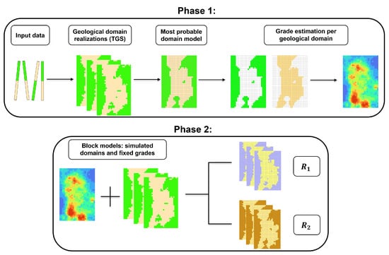
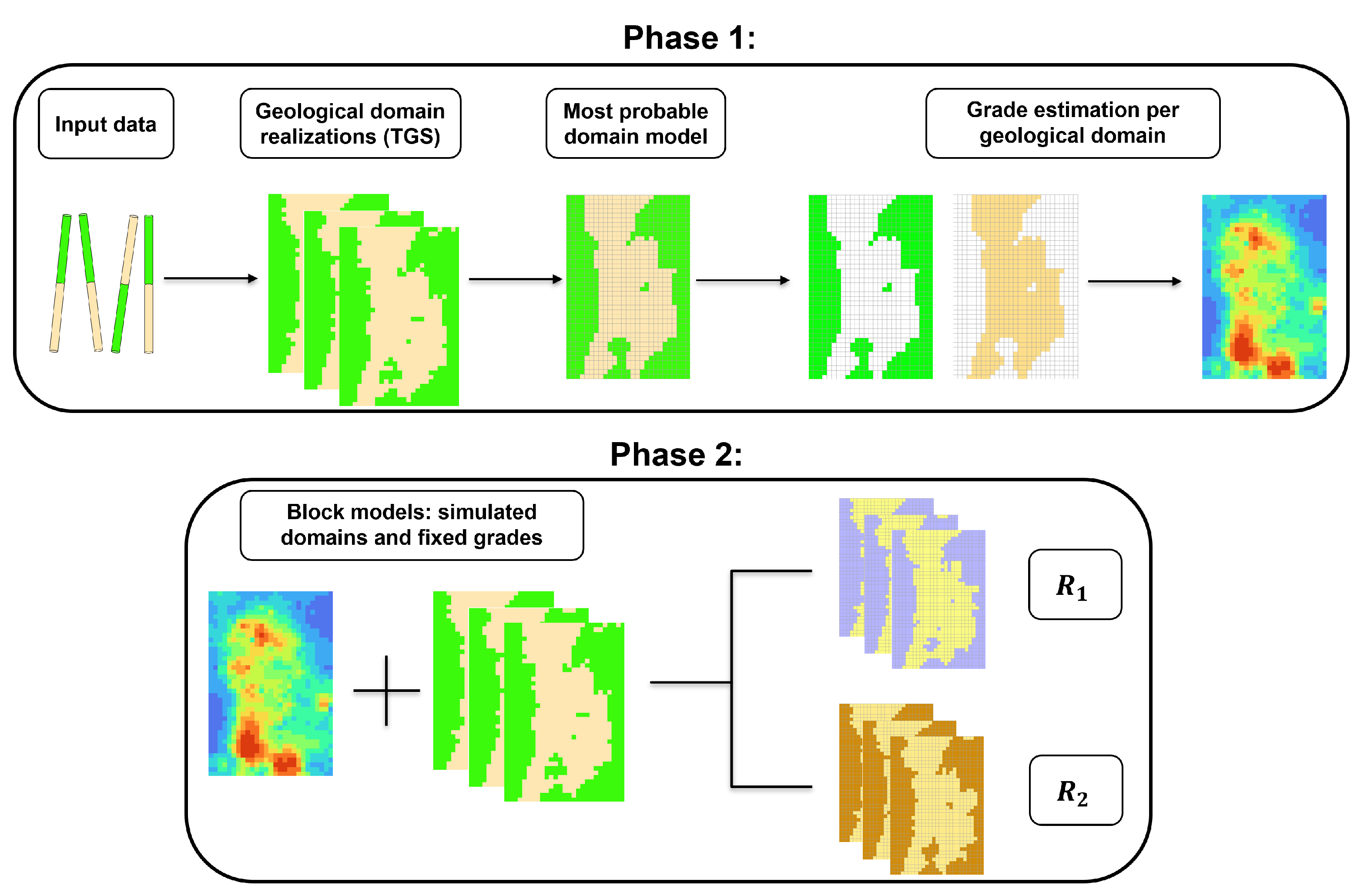
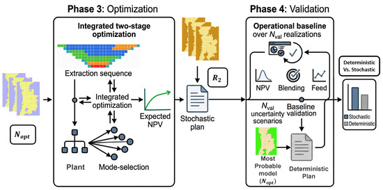
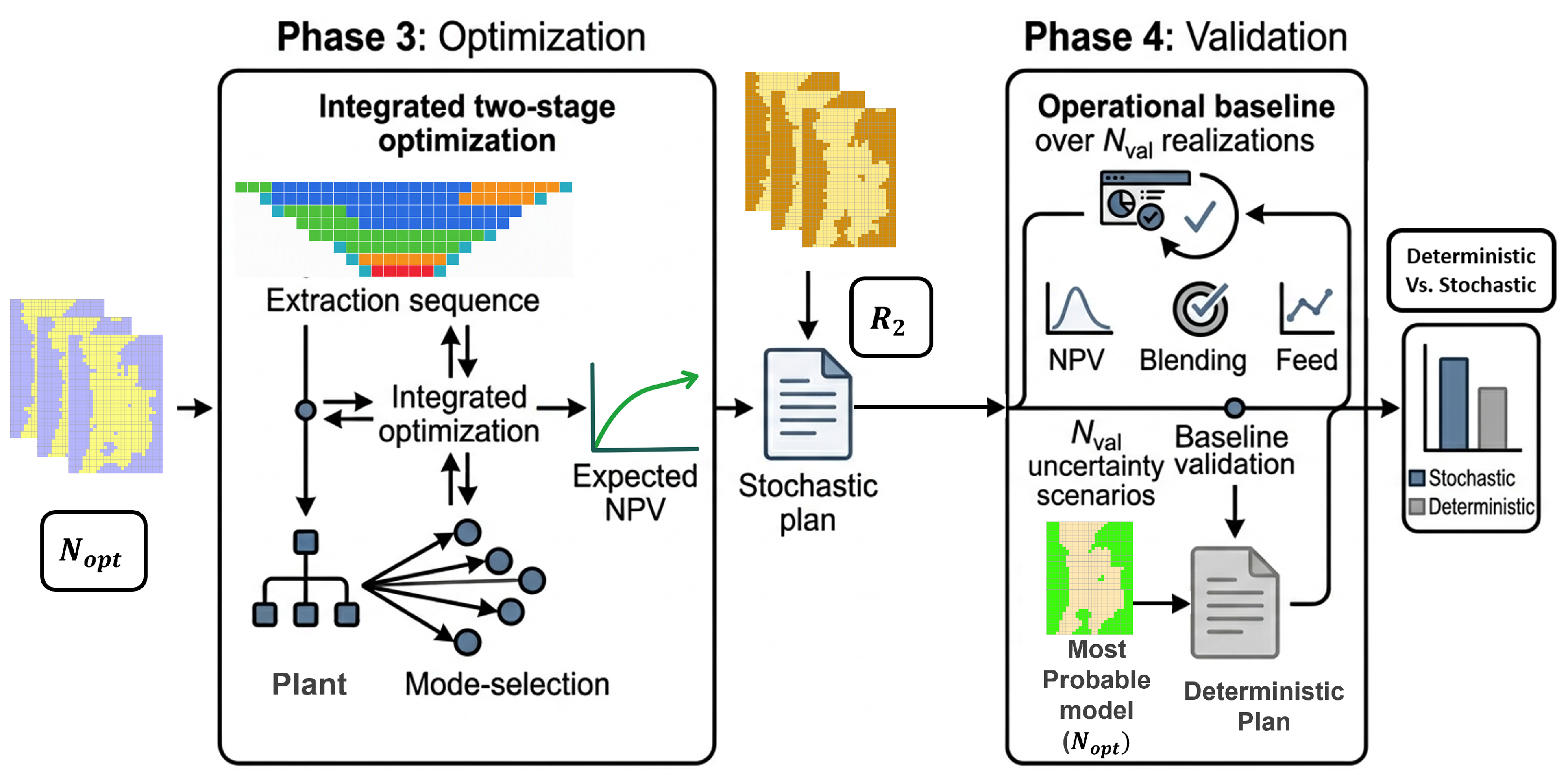
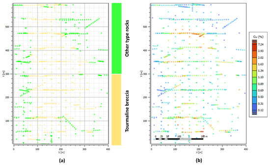
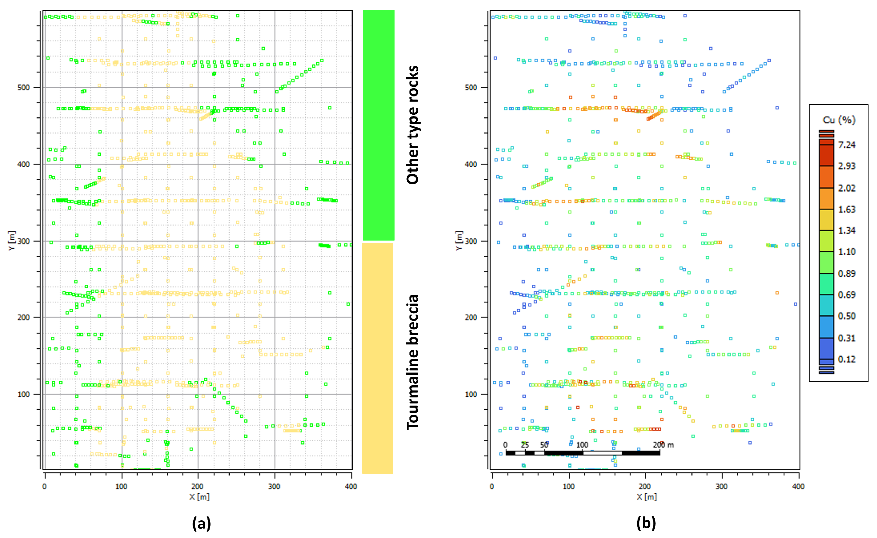
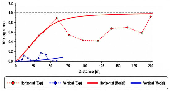
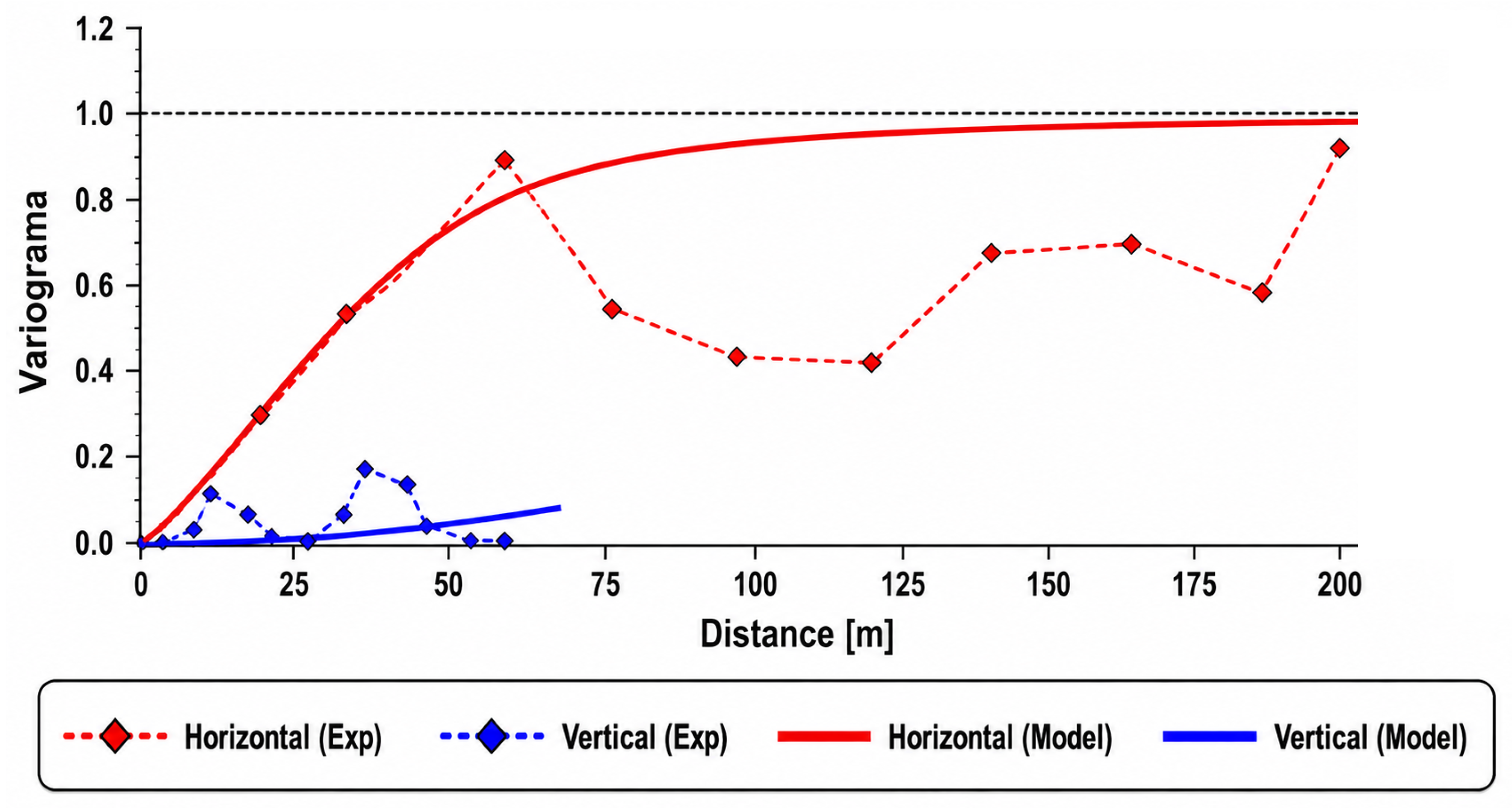
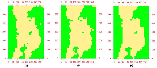
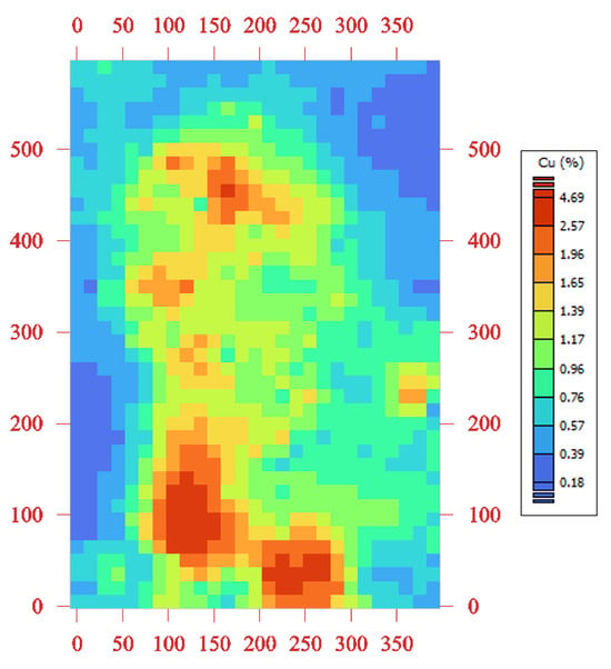
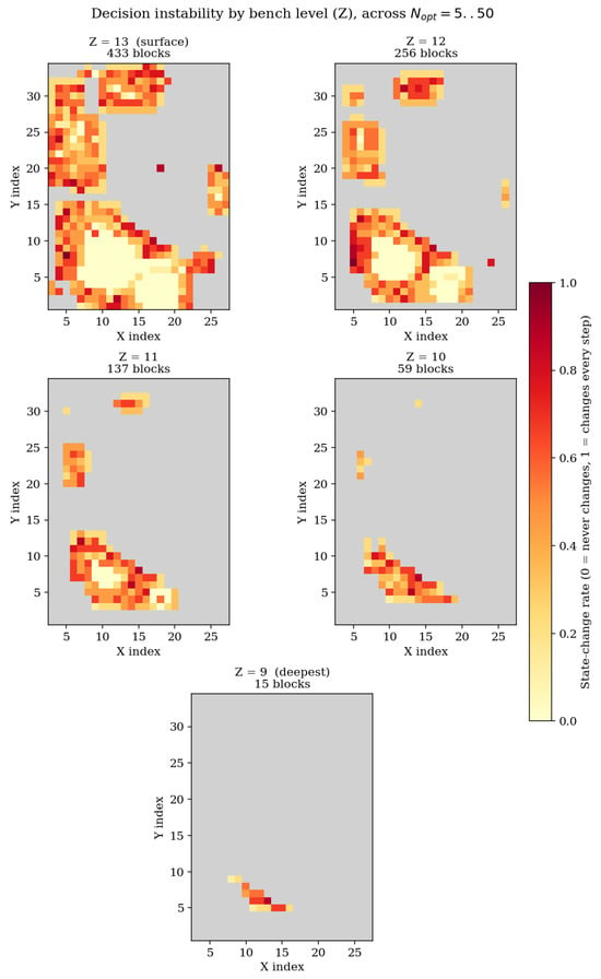
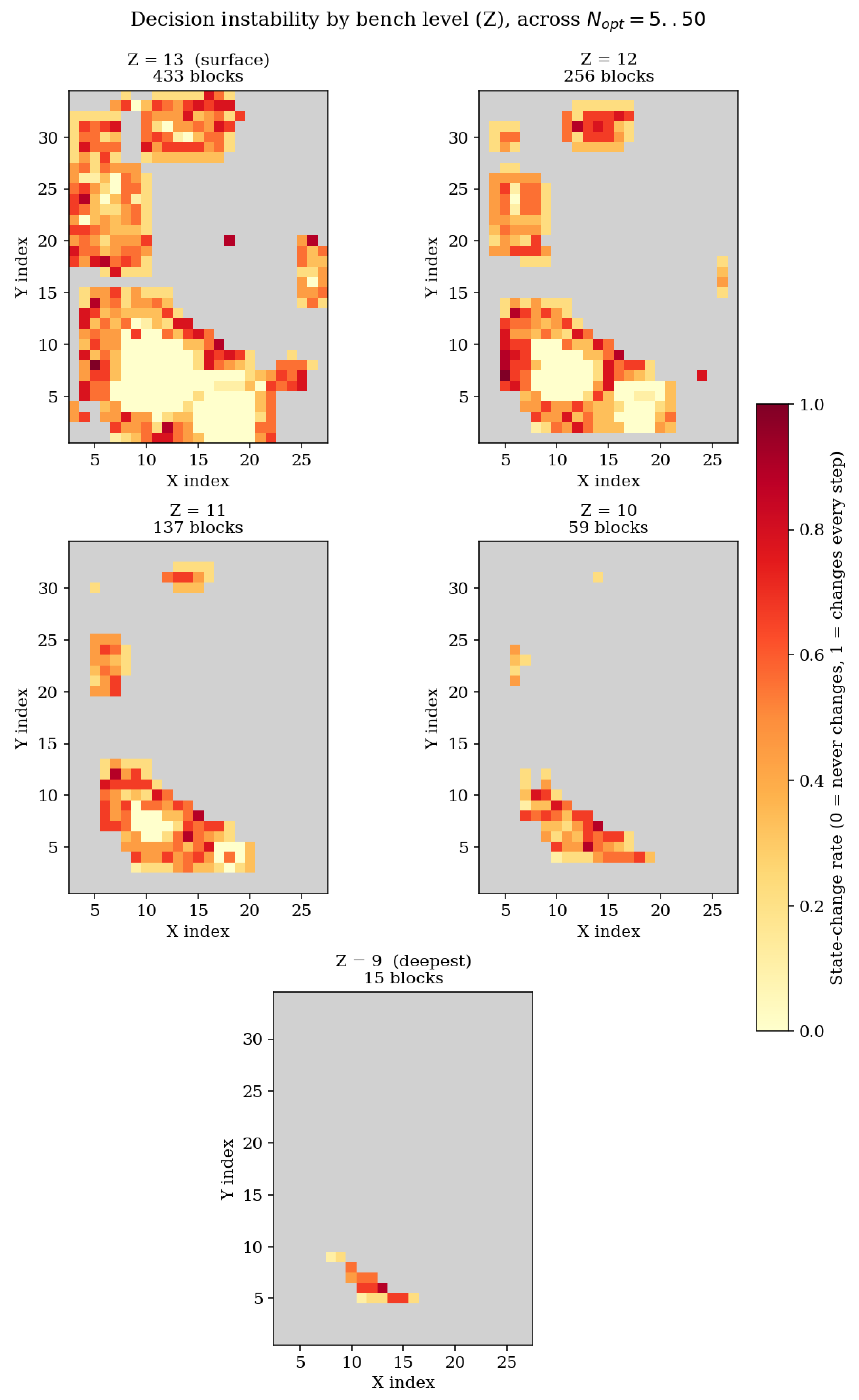
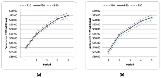
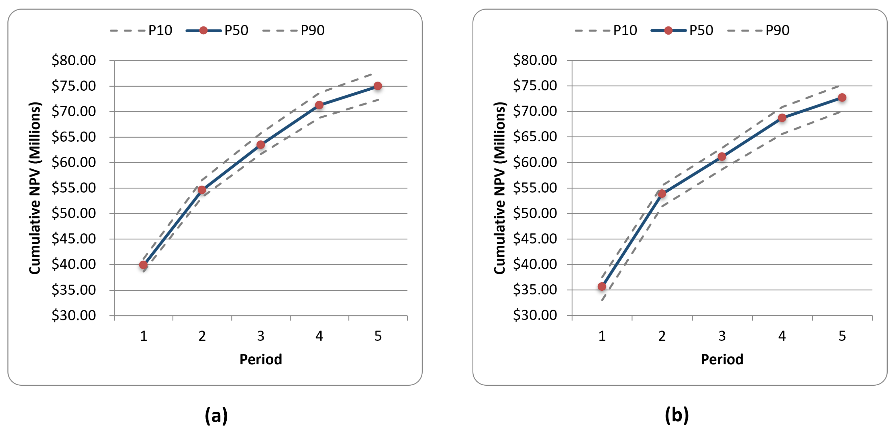
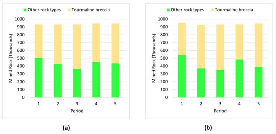
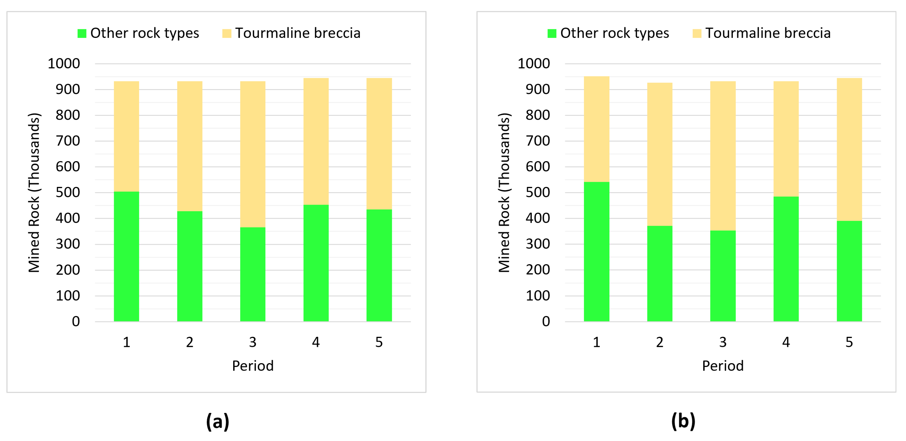
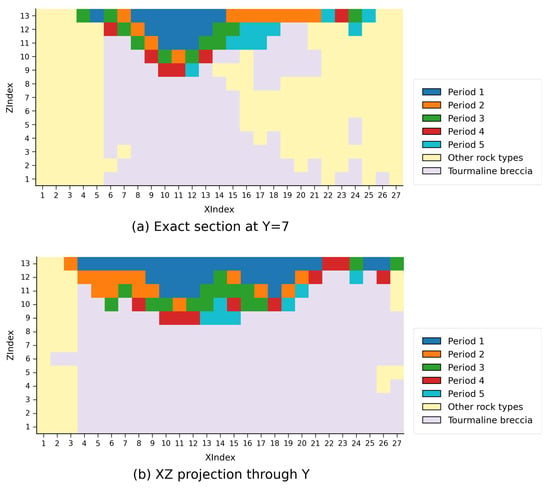
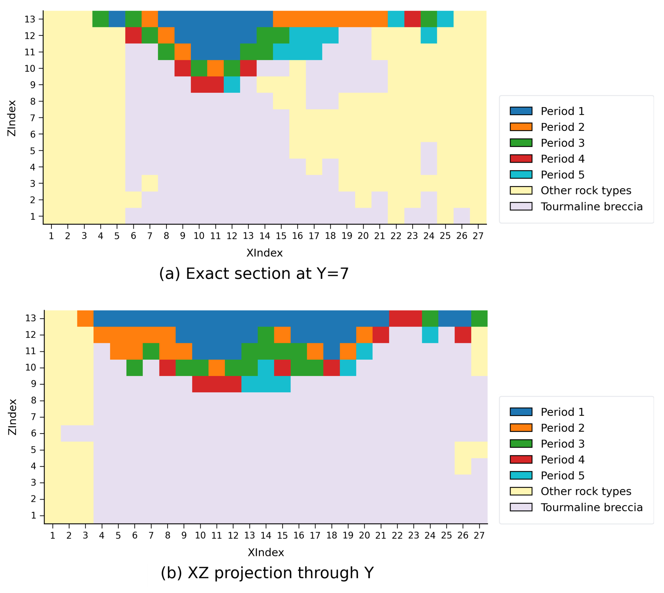
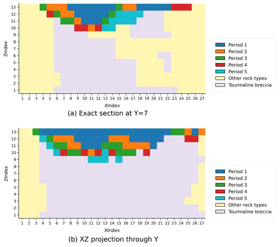
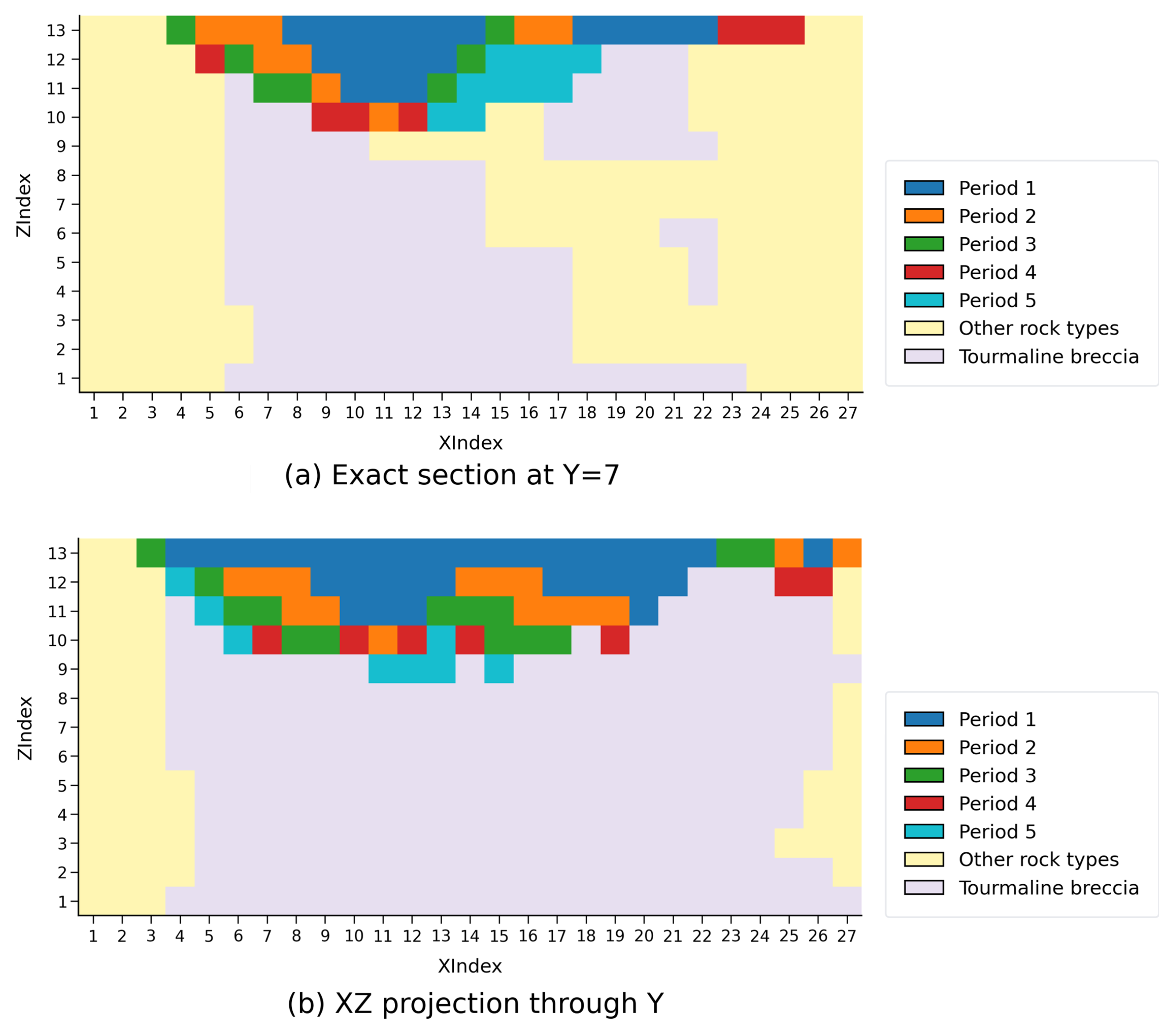
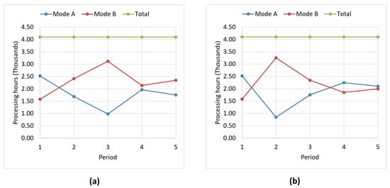
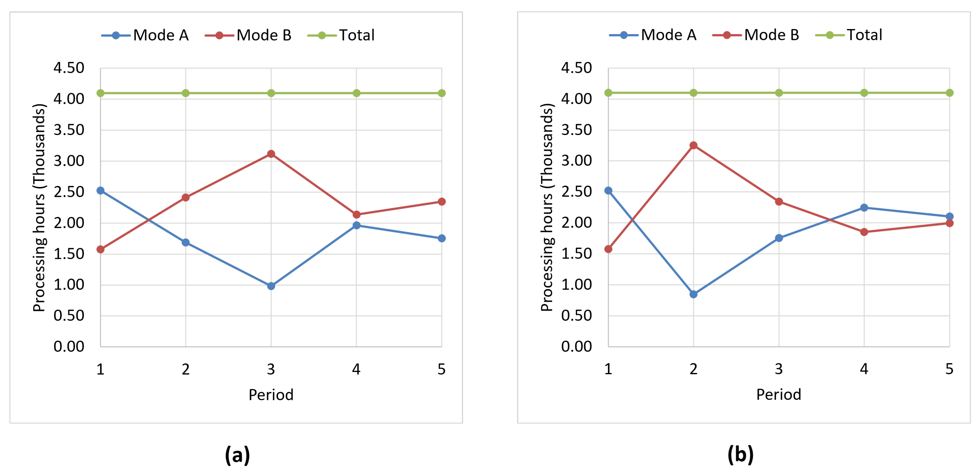
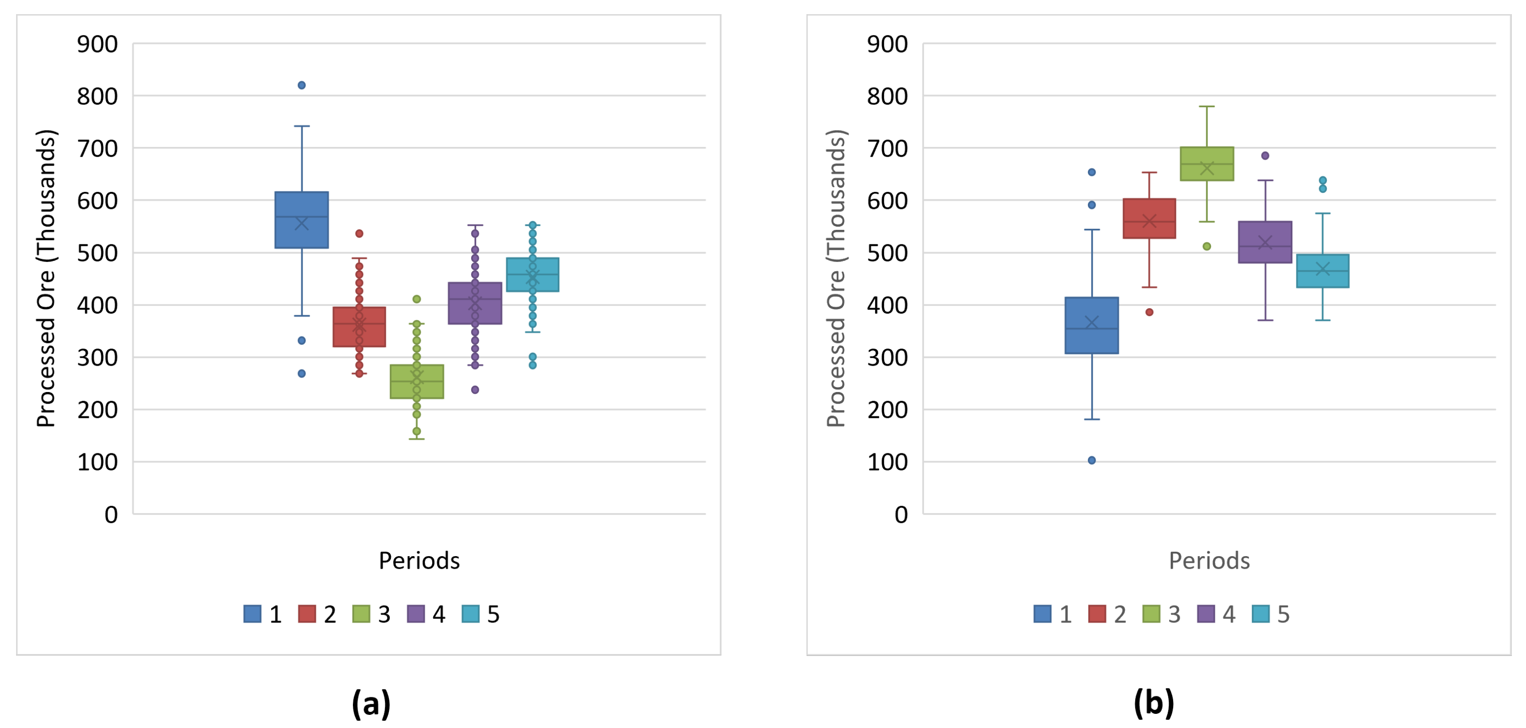
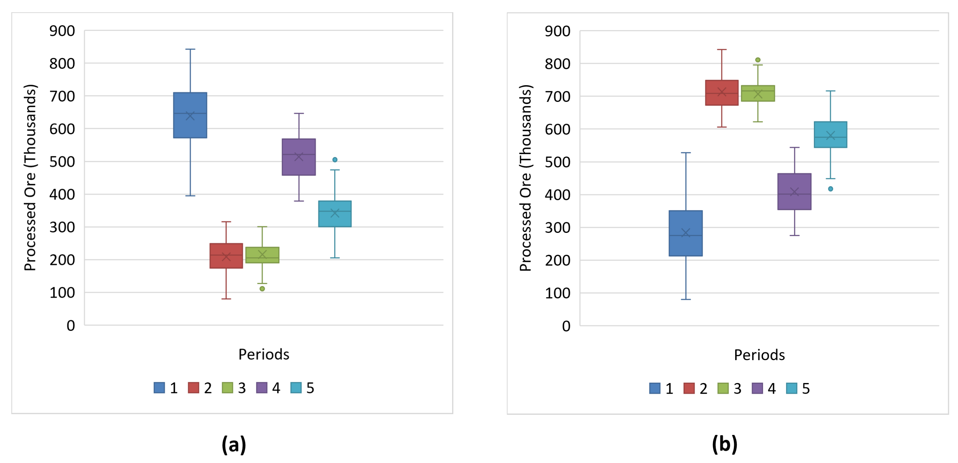

Disclaimer/Publisher’s Note: The statements, opinions and data contained in all publications are solely those of the individual author(s) and contributor(s) and not of MDPI and/or the editor(s). MDPI and/or the editor(s) disclaim responsibility for any injury to people or property resulting from any ideas, methods, instructions or products referred to in the content. |
© 2026 by the authors. Licensee MDPI, Basel, Switzerland. This article is an open access article distributed under the terms and conditions of the Creative Commons Attribution (CC BY) license.