Medium-Term Planning of Mining Complexes with Explicit Shovel Tracking and Processing Plant Uncertainty

Abstract

Simultaneous and stochastic optimization of open-pit mining complexes at the medium-term level aims to maximize expected profits, manage technical risk for integrated value chains, and enhance the operational feasibility of the long-term plan while still meeting its targets to achieve long-term value. To address two key operational feasibility challenges over a twelve-month horizon, the proposed framework integrates two features that provide a more detailed operational evaluation during decision-making than existing methods. The first involves explicit tracking of shovel movements to align optimized extraction sequences with the operational capabilities of loading equipment. The second uses high-order simulation to produce probability distributions for processing plant responses based on geometallurgical properties of the material being scheduled and selected operating modes. To efficiently optimize schedules with this detailed evaluation, a solution method is proposed using an online machine learning model to rank moves in a metaheuristic search procedure. The framework is demonstrated using a gold mining complex and results show realistic extraction sequences with an increase in metal production and cashflow when compared to a regression-based processing model.

1. Introduction

Simultaneous stochastic optimization of mining complexes aims to maximize profits from the sale of commodities produced by integrated mineral value chains while managing risk associated with uncertainty in key inputs [1,2,3,4,5,6]. Mine planning is typically done at several distinct time levels. Long-term plans maximize discounted cashflows over the project lifetime whereas medium- and short-term plans aim to incorporate operational details into the schedule while meeting long-term targets [7,8,9,10]. In terms of time granularity, long-term planning uses years as periods while medium-term planning considers quarters or months, and short-term planning examines weeks or days. The present work incorporates operational details related to the movement sequences of loading equipment and processing plant performance into the medium-term optimization to strengthen the connection between long-term project value and these aspects of operational feasibility. The former is achieved using a novel method for tracking and optimizing shovel hours used in the schedule and the latter is done by applying the high-order simulation method for processing performance developed by de Carvalho and Dimitrakopoulos [11].

Ensuring equipment access and minimizing unnecessary movement of loading equipment are key operational details that need to be handled during planning. Conventional long-term planning methods ensure schedules are feasible by using a minimum mining width during pushback design [12], but panels defined by pushbacks are not reflective of actual mining selectivity. Methods using direct block scheduling have included smoothness in the objective function, applying penalties when adjacent blocks are not mined in the same period [13]. While this approach is practical for long-term planning, it is a rough approximation for shovel feasibility as it ignores the number of shovels working in the mine and the distance between disconnected mining blocks. Medium-term planning requires a more precise assessment to guarantee operational feasibility. Both and Dimitrakopoulos [9] optimize monthly assignments of shovels to mining areas to minimize their movement, but only considering large areas ignores the feasibility of local extraction sequences. Matamoros and Dimitrakopoulos [14] use horizontal precedence constraints to control the extraction sequence but this may be overly restrictive, especially at the medium-term level. Not aligning medium-term extraction sequences with the operational behaviour of loading equipment is problematic because the optimization would therefore prefer a schedule that meets its flawed objective function over a different schedule that may perform better in reality. The proposed framework is aligned with operations by examining the geometry of the extraction sequence, optimizing the assignments of scheduled blocks to shovels, explicitly tracking the number of hours used by each shovel, and ensuring these are below the available limit.

Processing plant performance is also critical to the operational success of a mining complex. Because processing responses such as grindability or metal recovery depend on feed material properties, improving the framework that models processing plants during schedule optimization enables more reliable production forecasting and better decision-making. Both and Dimitrakopoulos [15] implement machine learning models to estimate responses including mill throughput based on the primary attributes of materials being blended and processed. They use proportional data to represent spatial attributes which cannot be averaged linearly [16,17]. However, there is significant uncertainty in these processing performance relationships due to the variability of operating conditions that deterministic estimation cannot characterize. Coward and Dowd [18] and Jiang and Dimitrakopoulos [19] generate stochastic functions for processing responses that follow a Gaussian distribution, but Gaussian or other parametrized distributions may not be suitable for all data. De Carvalho and Dimitrakopoulos [11] instead use high-order simulation [20,21] to simulate responses given the properties of the current batch of feed material and both the properties and responses of previous batches. The method extracts high-order cumulants from historical production data and reproduces their statistics without assuming any shape in the distribution or response function. However, the authors do not consider operating modes of processing facilities as conditioning data for the simulations. Operating mode decisions such as screen aperture setting or grinding mill method are critical to processing performance and have been included as decision variables in several mine planning frameworks [2,3,22,23,24]. The present work extends the use of the mentioned high-order simulation method to also consider operating mode decisions as conditioning data for simulating processing responses and applies it to the context of medium-term planning.

Simultaneous stochastic optimization of mining complexes requires metaheuristic algorithms [3,4,25], and newer methods have incorporated machine learning (ML) to accelerate these algorithms [10,26,27,28]. Including explicit shovel tracking and processing response simulation adds computation time to each solution evaluation, making the proposed framework an expensive optimization problem [29]. Such problems can benefit from ML surrogate models to efficiently manage expensive evaluations during the metaheuristic search. The present work follows research that uses ML models to rank different neighbours to inform the search order and improve search efficiency [30,31].

The framework proposed in this paper incorporates explicit shovel tracking and processing response uncertainty into the optimization of extraction sequencing, destination policy, process stream utilization and operating mode decisions for medium-term schedules of mining complexes. Supply uncertainty is considered through geostatistical realizations of the deposits while processing responses are simulated during the optimization based on blended feed materials and chosen operating modes in the schedule. The medium-term plan is required to fulfil the long-term extraction sequence for compliance. A solution method based on iterated local search [32] with ML-guidance that ranks search perturbations is developed to efficiently optimize the schedule. The following section presents the proposed optimization framework and supporting methods. Next, a case study is shown at a gold mining complex. Finally, conclusions and future research directions are discussed.

2. Methods

This section presents the methods that enable the simultaneous stochastic optimization of medium-term schedules for mining complexes with explicit shovel tracking and processing plant uncertainty. First, the stochastic integer programming (SIP) formulation which is an extension of the generalized simultaneous stochastic optimization of mining complexes [4] is presented. Following this is the approach used to explicitly track shovel hours and subsequently the high-order simulation method for processing responses. Finally, the ML-guided metaheuristic solution method is presented.

2.1. Stochastic Integer Programming Formulation

Table 1, Table 2 and Table 3 outline the notation used in the SIP formulation.

Table 1. List of sets and indices.

Notation	Definition
$p\in \mathbb{P}$	Primary attributes which represent quantities (e.g., tonnage, metal quantity) that flow through the mining complex
$h\in \mathbb{H}$	Hereditary attributes which account for information (e.g., blended grades, energy consumption, costs) that does not flow through the mining complex
$t\in \mathbb{T}$	Time periods
$s\in \mathbb{S}$	Stochastic orebody scenarios
$r\in \mathcal{R}$	Stochastic scenarios for process responses
$m\in \mathcal{M}$	Mines
$l\in {\mathbb{L}}_m$	Shovels working in mine $m$
$b\in {\mathbb{B}}_m$	Blocks in mine m
$c\in \mathcal{C}$	Clusters of material in mining complex
$i,j\in \mathcal{S}$	Stockpiling facilities
$i,j\in \mathcal{P}$	Non-stockpiling processing facilities
$\mathcal{N}=\mathcal{S}\cup \mathcal{P}\cup \mathcal{M}$	Set of nodes that describe the mining complex
${\mathcal{I}}_i$	Possible material sources for node i
${\mathcal{O}}_i$	Possible material destinations from node i
$a\in {\mathbb{A}}_i$	Operating modes at facility $i$
$q\in {\mathbb{Q}}_i$	Set of products made at facility $i$

Table 2. List of decision variables.

Notation	Definition
$x_{bt}\in \left\{0,1\right\}$	Mine block b in period t
$z_{cjt}\in \left\{0,1\right\}$	Send cluster $c$ to destination $j$ in period $t$
$y_{qijtsr}\in \left[0,1\right]$	Send portion of material product $q$ from source $i$ to destination $j$ in period $t,$ orebody scenario $s,$ and response scenario $r$
$u_{iat}\in \left\{0,1\right\}$	Use operating mode $a$ at location $i$ in period $t$
$v_{pijtsr}\ge 0$	Value of primary attribute $p$ moving from source $i$ to destination $j$ in period $t,$ orebody scenario $s,$ and response scenario $r$
$v_{hitsr}\ge 0$	Value of hereditary attribute $h$ at location $i$ in period $t,$ orebody scenario $s,$ and response scenario $r$
${\lambda }_{pqitsr}\in \left[0,1\right]$	Portion of primary attribute $p$ recovered in product $q$ at location $i$ in period $t,$ orebody scenario $s,$ and response scenario $r$
$d_{hitsr}^{+},d_{hitsr}^{-}\ge 0$	Upward and downward deviations from production target $h$ at location $i$ in period $t,$ scenario $s,$ and response scenario $r$
$d_{hisr}^{\mathrm{L}\mathrm{T}+},d_{hisr}^{\mathrm{L}\mathrm{T}-}\ge 0$	Upward and downward deviations from end-of-year production target $h$ at location $i,$ scenario $s,$ and response scenario $r$
${\tau }_{mlt}\ge 0$	Time used by shovel $l$ in mine $m$ and period $t$
$d_{mlt}^{+}\ge 0$	Upward deviation from available hours for shovel $l$ in mine $m$ and period $t$

Table 3. List of input parameters.

Notation	Definition
${\theta }_{bcs}\in \left\{0,1\right\}$	Indicator showing if a block $b$ belongs to cluster $c$ in scenario $s$
${\beta }_{pbs}$	Simulated value for primary attribute $p$ in block $b$ and scenario $s$
$p_{hit}$	Discounted value per unit of hereditary attribute $h$ at location $i$ in period $t$
$f_{pqi}\left(\mathbf{v},\mathbf{u}\right)$	User-defined functions that defines the recovery of product $q$ at location $i$ based on primary attribute values $\mathbf{v}$ and selected operating modes $\mathbf{u}$
$f_{hi}\left(\mathbf{v},\mathbf{u}\right)$	User-defined functions that defines the hereditary attribute $h$ at location $i$ based on primary attribute values $\mathbf{v}$ and selected operating modes $\mathbf{u}$
$U_{hit},L_{hit}$	Upper and lower production targets for attribute $h$ at location $i$ in period $t$
$c_{hit}^{+},c_{hit}^{-}$	Risk-discounted cost of upward and downward deviations from production targets associated with hereditary attribute $h$ at location $i$ in period $t$
$g_{iah}^{+},g_{iah}^{-}$	Multipliers for the impact of operating mode $a$ at location $i$ on the upper and lower targets of hereditary attribute $h$
$U_{hi}^{\mathrm{L}\mathrm{T}},L_{hi}^{\mathrm{L}\mathrm{T}}$	Upper and lower end-of-year production targets for attribute $h$ at location $i$
$c_{hi}^{\mathrm{L}\mathrm{T}+},c_{hi}^{\mathrm{L}\mathrm{T}-}$	Cost of upward and downward deviations from end-of-year production targets associated with hereditary attribute $h$ at location $i$
$U_{mlt}$	Number of available hours for shovel $l$ in mine $m$ and period $t$
$c_t^l$	Risk-discounted cost of upward deviations from number of available hours for shovels in period $t$

The SIP optimizes the following objective function:

$$\begin{gathered} \max {\displaystyle \frac{1}{\left|\mathbb{S}\right|\cdot \left|\mathcal{R}\right|}}\sum _{s\in \mathbb{S}}\sum _{i\in \mathcal{N}}\sum _{h\in \mathbb{H}}\sum _{t\in \mathbb{T}}\sum _{r\in \mathcal{R}}\left(\underset{\mathrm{C}\mathrm{a}\mathrm{s}\mathrm{h}\mathrm{f}\mathrm{l}\mathrm{o}\mathrm{w}}{\underbrace{p_{hit}\cdot v_{hitsr}}}-\underset{\mathrm{P}\mathrm{e}\mathrm{n}\mathrm{a}\mathrm{l}\mathrm{t}\mathrm{i}\mathrm{e}\mathrm{s}}{\underbrace{c_{hit}^{+}\cdot d_{hitsr}^{+}-c_{hit}^{-}\cdot d_{hitsr}^{-}}}\right) \\ -{\displaystyle \frac{1}{\left|\mathbb{S}\right|\cdot \left|\mathcal{R}\right|}}\sum _{s\in \mathbb{S}}\sum _{i\in \mathcal{N}}\sum _{h\in \mathbb{H}}\sum _{r\in \mathcal{R}}\left(\underset{\mathrm{E}\mathrm{n}\mathrm{d}-\mathrm{o}\mathrm{f}-\mathrm{Y}\mathrm{e}\mathrm{a}\mathrm{r} \mathrm{P}\mathrm{e}\mathrm{n}\mathrm{a}\mathrm{l}\mathrm{t}\mathrm{i}\mathrm{e}\mathrm{s}}{\underbrace{c_{hi}^{\mathrm{L}\mathrm{T}+}\cdot d_{hisr}^{\mathrm{L}\mathrm{T}+}+c_{hi}^{\mathrm{L}\mathrm{T}-}\cdot d_{hisr}^{\mathrm{L}\mathrm{T}-}}}\right)-\sum _{m\in \mathcal{M}}\sum _{l\in {\mathbb{L}}_m}\sum _{t\in \mathbb{T}}\underset{\mathrm{S}\mathrm{h}\mathrm{o}\mathrm{v}\mathrm{e}\mathrm{l} \mathrm{P}\mathrm{e}\mathrm{n}\mathrm{a}\mathrm{l}\mathrm{t}\mathrm{i}\mathrm{e}\mathrm{s}}{\underbrace{c_t^l\cdot d_{mlt}^{+}}} \end{gathered}$$

(1)

The first component counts the expected revenue and operating costs from production, transportation, and sale of products throughout the schedule over the set of scenarios formed by the orebody and processing response realizations. The second component tracks risk-discounted penalties which are applied to minimize the risk of not meeting production targets or capacities throughout the mining complex. The third component applies penalties to deviations from end-of-year targets. The fourth component applies additional penalties if the schedule requires the shovels to work more hours than are available.

The optimization is subject to constraints which are defined below. Additional constraints regarding slope stability and cluster-based destination policy are available in the formulation presented by Goodfellow and Dimitrakopoulos [4].

The reserve constraint ensures that every block is mined as it is assumed that the 12-month schedule will follow the design set by a long-term plan. This is one of the main links between long-term targets and the medium-term plan.

$$\sum _{t\in \mathbb{T}}{x}_{bt}=1\hspace{1em}\forall b\in {\mathbb{B}}_m,m\in \mathcal{M}$$

(2)

The operating mode constraint requires that one operating mode is selected for each facility and each period.

$$\sum _{a\in {\mathbb{A}}_i}{u}_{iat}=1,\forall i\in \mathcal{P},t\in \mathbb{T}$$

(3)

Material flow constraints calculate the mass balance of materials flowing from mines, processors, and stockpiles.

$$\begin{gathered} v_{pmjtsr}=\sum _{b\in {\mathbb{B}}_m}\sum _{c\in \mathcal{C}}{\beta }_{pbs}\cdot {\theta }_{bcs}\cdot x_{bt}\cdot z_{cjt} \\ \forall p\in \mathbb{P},m\in \mathcal{M},j\in {\mathcal{O}}_m,t\in \mathbb{T},s\in \mathbb{S},r\in \mathcal{R} \end{gathered}$$

(4)

$$\begin{gathered} v_{pijtsr}=\sum _{k\in {\mathcal{I}}_i}{v}_{pkitsr}\sum _{q\in {\mathbb{Q}}_i}{\lambda }_{pqitsr}\cdot y_{qijtsr} \\ \forall p\in \mathbb{P},i\in \mathcal{P},j\in {\mathcal{O}}_i,t\in \mathbb{T},s\in \mathbb{S},r\in \mathcal{R} \end{gathered}$$

(5)

$$\begin{gathered} v_{pijtsr}=\left[\sum _{t^{\prime }=1}^{t-1}\sum _{k\in {\mathcal{I}}_i}{v}_{pki{t}^{\prime }sr}-\sum _{t^{\prime }=1}^{t-1}\sum _{k\in {\mathcal{O}}_i}{v}_{pik{t}^{\prime }sr}\right]\cdot \sum _{q\in {\mathbb{Q}}_i}{y}_{qijtsr} \\ \forall p\in \mathbb{P},i\in \mathcal{S},j\in {\mathcal{O}}_i,t\in \mathbb{T},s\in \mathbb{S},r\in \mathcal{R} \end{gathered}$$

(6)

Downstream flow constraints ensure that all incoming material needs to exit processors and no more than the available material can be reclaimed from stockpiles.

$$\sum _{j\in {\mathcal{O}}_i}{y}_{qijtsr}=1\hspace{1em}\forall i\in \mathcal{P},q\in {\mathbb{Q}}_i,t\in \mathbb{T},s\in \mathbb{S},r\in \mathcal{R}$$

(7)

$$\sum _{j\in {\mathcal{O}}_i}{y}_{qijtsr}\le 1\hspace{1em}\forall i\in \mathcal{S},q\in {\mathbb{Q}}_i,t\in \mathbb{T},s\in \mathbb{S},r\in \mathcal{R}$$

(8)

The byproduct constraint ensures that separation processes recover all the incoming mass in the created products. Product recoveries can be defined as a function (such as a stochastic simulator) of incoming primary attributes and any relevant operating mode decisions. Hereditary attributes can also be defined using any function of primary attributes.

$$\sum _{q\in {\mathbb{Q}}_i}{\lambda }_{pqitsr}=1\hspace{1em}\forall p\in \mathbb{P},i\in \mathcal{P},t\in \mathbb{T},s\in \mathbb{S},r\in \mathcal{R}$$

(9)

$${\lambda }_{pqitsr}=f_{pqi}\left(\mathbf{v},\mathbf{u}\right)\hspace{1em}\forall p\in \mathbb{P},i\in \mathcal{P},q\in {\mathbb{Q}}_i,t\in \mathbb{T},s\in \mathbb{S},r\in \mathcal{R}$$

(10)

$$v_{hitsr}=f_{hi}\left(\mathbf{v},\mathbf{u}\right)\hspace{1em}\forall h\in \mathbb{H},i\in \mathcal{N},t\in \mathbb{T},s\in \mathbb{S},r\in \mathcal{R}$$

(11)

Operating modes at processing facilities may impact production targets, so deviations are calculated based on the base targets and operating modes selected.

$$v_{hitsr}-d_{hitsr}^{+}\le U_{hit}\sum _{a\in {\mathbb{A}}_i}{u}_{iat}\cdot g_{iah}^{+}\hspace{1em}\forall h\in \mathbb{H},i\in \mathcal{P},t\in \mathbb{T},s\in \mathbb{S},r\in \mathcal{R}$$

(12)

$$v_{hitsr}+d_{hitsr}^{-}\ge L_{hit}\sum _{a\in {\mathbb{A}}_i}{u}_{iat}\cdot g_{iah}^{-}\hspace{1em}\forall h\in \mathbb{H},i\in \mathcal{P},t\in \mathbb{T},s\in \mathbb{S},r\in \mathcal{R}$$

(13)

Deviations from end-of-year targets set by the long-term plan need to be calculated based on the sums of hereditary attributes accumulated throughout the schedule.

$$\sum _{t\in \mathbb{T}}{v}_{hitsr}-d_{hisr}^{\mathrm{L}\mathrm{T}+}\le U_{hi}^{\mathrm{L}\mathrm{T}}\hspace{1em}\forall h\in \mathbb{H},i\in \mathcal{P},s\in \mathbb{S},r\in \mathcal{R}$$

(14)

$$\sum _{t\in \mathbb{T}}{v}_{hitsr}+d_{hisr}^{\mathrm{L}\mathrm{T}-}\ge L_{hi}^{\mathrm{L}\mathrm{T}}\hspace{1em}\forall h\in \mathbb{H},i\in \mathcal{P},s\in \mathbb{S},r\in \mathcal{R}$$

(15)

Finally, the deviations in shovel hours are calculated based on the time to execute the schedule and the predefined number of available hours per shovel. The explicit calculation of the hours used by each shovel is explained in the following section.

$${\tau }_{mlt}-d_{mlt}^{+}\le U_{mlt}\hspace{1em}\forall m\in \mathcal{M},l\in {\mathbb{L}}_m,t\in \mathbb{T}$$

(16)

2.2. Explicit Shovel Tracking

To incorporate explicit shovel tracking for the schedule of the mining complex, the time used by each shovel $\left({\tau }_{m,l,t}\right)$ needs to be calculated as a function of the selected extraction sequence. This includes the time required for each block to be mined as well as the time required for any transportation of the shovels between non-adjacent blocks. Because the schedule aims to minimize shovel hour deviations, the proposed framework treats the overall formulation as a bi-level optimization problem where the upper level optimizes the schedule for the mining complex, and the lower level aims to find the most time-efficient shovel sequence. The lower-level shovel sequence is optimized for each solution that is evaluated during the upper-level schedule optimization.

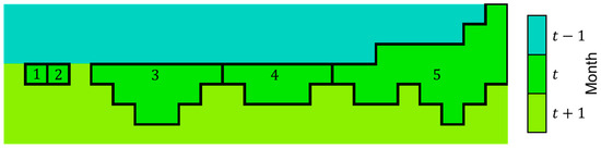
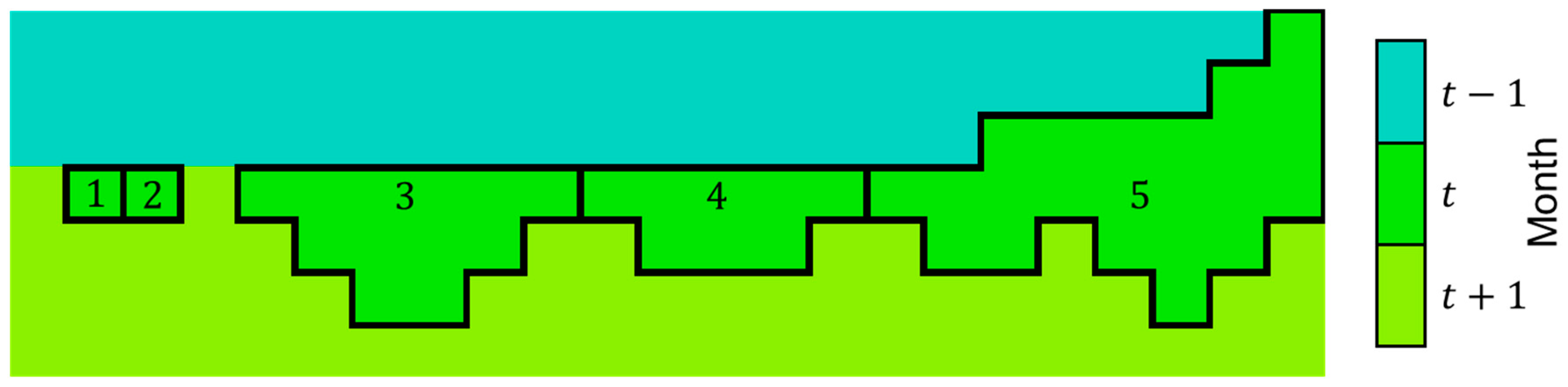
To reduce problem complexity, blocks that are contiguous and scheduled in the same period are grouped into units. Let the set $N_{m,t}$ include all the units of blocks in mine $m$ scheduled in period $t$. Let the mining unit $n_b\in N_{m,t}$ be defined as the smallest grouping of blocks that includes block $b$ such that no unit in $N_{m,t}$ depends on another unit in $N_{m,t}$ for slope stability. An example of the formation of five units is shown in Figure 1.

Figure 1. Example side view of mining units in a vertical 2D extraction sequence.

The shovel sequence optimization is modelled with the decision variable, ${\psi }_{n,l,t,k}\in \left\{0, 1\right\}$ which equals 1 if unit $n$ is mined in period $t$ and assigned to shovel $l$ in the $k^{\mathrm{t}\mathrm{h}}$ position of its sequence. The set ${\mathbb{K}}_{l,t}$ of positions for shovel $l$ in period $t$ is sufficiently large such that the sequence will never fill it entirely. The objective function is defined as follows:

$$\min \sum _{m\in \mathcal{M}}\sum _{l\in {\mathbb{L}}_m}\sum _{t\in \mathbb{T}}{c}_t^l\cdot d_{m,l,t}^{+}$$

(17)

The time used for each shovel to execute its assigned sequence includes the time required to extract each unit $\left(T_n^{dig}\right)$ and the time to move between each unit in the sequence $\left(T_{n,n^{\prime }}^{\mathrm{m}\mathrm{o}\mathrm{v}\mathrm{e}}\right)$,

$$\begin{gathered} {\tau }_{m,l,t}=\sum _{n\in N_{m,t-1}}\sum _{n^{\prime }\in N_{m,t}}{T}_{n,n^{\prime }}^{\mathrm{m}\mathrm{o}\mathrm{v}\mathrm{e}}\cdot {\pi }_{n,l,t-1}\cdot {\psi }_{n^{\prime },l,t,1}+\sum _{n\in N_{m,t}}\sum _{n^{\prime }\in N_{m,t}}\sum _{k=1}^{\left|{\mathbb{K}}_{l,t}\right|-1}{T}_{n,n^{\prime }}^{\mathrm{m}\mathrm{o}\mathrm{v}\mathrm{e}}\cdot {\psi }_{n,l,t,k}\cdot {\psi }_{n^{\prime },l,t,k+1} \\ +\sum _{n\in N_{m,t}}\sum _{k\in {\mathbb{K}}_{l,t}}{T}_n^{\mathrm{d}\mathrm{i}\mathrm{g}}\cdot {\psi }_{n,l,t,k}\hspace{1em}\forall m\in \mathcal{M},l\in {\mathbb{L}}_m,t\in \mathbb{T} \end{gathered}$$

(18)

where ${\pi }_{n,l,t}\in \left\{0, 1\right\}$ is a variable that equals 1 if unit $n$ is the last sequenced unit for shovel $l$ in period $t$. This allows the calculation to consider the inter-period moving time. In the first period, the initial locations $\left({\pi }_{n,l,0}\right)$ are defined a priori.

Sequencing constraints ensure that each unit is assigned to one shovel and one sequence position in the period it is being mined, and that no two units can be assigned to the same shovel and sequence position. An additional constraint ensures the contiguity of the shovel sequences.

$$\sum _{l\in {\mathbb{L}}_m}\sum _{k\in {\mathbb{K}}_{l,t}}{\psi }_{n,l,t,k}=1\hspace{1em}\forall m\in \mathbb{M},n\in N_{m,t},t\in \mathbb{T}$$

(19)

$$\sum _{n\in N_{m,t}}{\psi }_{n,l,t,k}\le 1\hspace{1em}\forall m\in \mathcal{M},l\in {\mathbb{L}}_m,t\in \mathbb{T},k\in {\mathbb{K}}_{l,t}$$

(20)

$$\sum _{n\in N_{m,t}}{\psi }_{n,l,t,k}\ge \sum _{n\in N_{m,t}}{\psi }_{n,l,t,k+1}\hspace{1em}\forall m\in \mathcal{M},l\in {\mathbb{L}}_m,t\in \mathbb{T},k\in \left\{1,\dots ,\left|{\mathbb{K}}_{l,t}\right|-1\right\}$$

(21)

Finally, the last unit in each monthly sequence is identified.

$${\pi }_{n,l,t}\ge {\psi }_{n,l,t,k}-\sum _{n^{\prime }\in N_{m,t}}{\psi }_{n^{\prime },l,t,k+1}\hspace{1em}\forall n\in N_{m,t},m\in \mathcal{M},l\in {\mathbb{L}}_m,t\in \mathbb{T},k\in \left\{1,\dots ,\left|{\mathbb{K}}_{l,t}\right|-1\right\}$$

(22)

Even with blocks grouped into units, finding the minimum-penalty shovel sequences is a nontrivial optimization problem that needs to be solved for every iteration of the upper-level schedule optimization during the metaheuristic search procedure. To maintain computational tractability, a nearest neighbour heuristic is used to construct a greedy solution. It begins at the first period with empty shovel sequences. It considers assigning each unit in the first period to the end of each shovel sequence and calculates the resulting total penalties and total time used. It selects the assignment that yields the lowest total penalties, or in the case of a tie, the assignment which results in the lowest total time used. The algorithm proceeds until all units in the first period are assigned, then continues to the next period until all periods are finished. The pseudocode for this algorithm is shown in Appendix A. It is worth noting that this algorithm does not guarantee optimality to the lower-level problem. As a result, the upper-level problem, which is optimized using the lower-level solution as an evaluation metric, will be steered towards solutions that perform well on this algorithm even though other solutions may be more theoretically optimal. However, one consolation is that within the evaluation of a single schedule, suboptimal shovel sequences can only be considered conservative, which is more acceptable for operations than the alternative.

2.3. Simulating Processing Responses

The formulation presented in Section 2.1 allows any functions $\left(f_{hi}\left(\cdot \right),f_{pqi}\left(\cdot \right)\right)$ to represent the processes that yield hereditary and material product recovery, respectively. These functions can be simulators which generate realizations on the set of stochastic processing scenarios, $\mathcal{R}$. De Carvalho and Dimitrakopoulos [11] develop a method for simulating processing responses with high-order statistics which is applied here. Without loss of generality, both types of simulated processing responses can be represented by a stationary and ergodic random function $\mathbf{R}=\left[R_1,\dots ,R_N\right]$ where $N$ is the number of different responses being simulated. Conditioning data can include relevant primary material properties and processing facility operating modes. These are represented by the random function $\mathbf{P}=\left[P_1,\dots ,P_M\right]$ where $M$ is the number of conditioning variables. The vector $\left[r_1,\dots ,r_N\right]$ represents one realization which is sampled from the joint conditional probability density function (cpdf) $f\left(R_1,\dots ,R_N|P_1,\dots ,P_M\right)$. The joint cpdf can be expressed as a product of univariate cpdfs [33] which enables sequential simulation of the random function:

$$f\left(R_1,\dots ,R_N|P_1,\dots ,P_M\right)=\prod _{n=1}^{N}f\left(R_n|\mathbf{P},R_1,\dots ,R_{n-1}\right)$$

(23)

The univariate cpdf can be decomposed using Bayes rule:

$$f\left(R_n|\mathbf{P},R_1,\dots ,R_{n-1}\right)={\displaystyle \frac{f\left(R_1,\dots ,R_n,\mathbf{P}\right)}{{\int }_{\mathcal{D}}f\left(R_1,\dots ,R_n,\mathbf{P}\right)d{R}_n}}\hspace{1em}\forall n\in \left\{1,\dots ,N\right\}$$

(24)

where $\mathcal{D}$ is domain defined as the possible values of $R_n$. The joint distribution can be approximated using high-order statistics by constructing a series of Legendre polynomials:

$$f\left(R_1,\dots ,R_n,\mathbf{P}\right)=\mathrm{f}\left(\mathbf{\Lambda }\right)\approx \sum _{{\mathsf{\alpha }}_{{\lambda }_1}=0}^{\omega }\dots \sum _{{\mathsf{\alpha }}_{{\lambda }_{\left|\mathbf{\Lambda }\right|}}=0}^{\omega }{L}_{{\alpha }_{{\lambda }_1},\dots ,{\alpha }_{{\lambda }_{\left|\mathbf{\Lambda }\right|}}}\cdot {\phi }_{{\alpha }_{{\lambda }_1}}\left({\mathbf{\Lambda }}_1\right)\cdot \dots \cdot {\phi }_{{\alpha }_{{\lambda }_{\left|\mathbf{\Lambda }\right|}}}\left({\mathbf{\Lambda }}_{\left|\mathbf{\Lambda }\right|}\right)$$

(25)

where $\mathbf{\Lambda }=\left[R_1,\dots ,R_n,\mathbf{P}\right]$ for the ease of notation, $L_{{\alpha }_{{\lambda }_1},\dots ,{\alpha }_{{\lambda }_{\left|\mathbf{\Lambda }\right|}}}$ is the Legendre coefficient that corresponds to the statistical orders denoted by the $\alpha$ indices, and ${\phi }_{\alpha }$ is the Legendre polynomial of order $\alpha$. The coefficients are calculated from available training data and convey the data’s high-order statistics:

$$L_{{\alpha }_{{\lambda }_1},\dots ,{\alpha }_{{\lambda }_{\left|\mathbf{\Lambda }\right|}}}\approx \mathbb{E}\left[{\phi }_{{\alpha }_{{\lambda }_1}}\left({\mathbf{\Lambda }}_1\right)\cdot \dots \cdot {\phi }_{{\alpha }_{{\lambda }_{\left|\mathbf{\Lambda }\right|}}}\left({\mathbf{\Lambda }}_{\left|\mathbf{\Lambda }\right|}\right)\right]$$

(26)

For simulating processing responses such as grinding mill energy consumption, screen separation ratios, or metal recovery from flotation, historical measurements can be used as training data to inform the high-order simulation process. This allows the simulator to extract high-order statistics from past data to inform the distribution of possible results for future periods being forecasted and optimized. Realizations are drawn by sampling from the constructed distribution after it is converted back to the conditional distribution using Equation (24). Simulating these responses sequentially in joint realizations $r\in \mathcal{R}$ allows the correlations between them to be considered. Conversely, the proposed framework assumes each period $t\in \mathbb{T}$ and each orebody scenario $s\in \mathbb{S}$ are independent and therefore processing performance attributes are simulated for each period and orebody scenario separately. More detailed explanations and theoretical proofs can be found in several published works [11,20,21].

2.4. Solution Method for Optimizing Medium-Term Schedules

The proposed SIP for medium-term scheduling requires the shovel sequence optimization and the high-order simulation of processing responses for each evaluation of the objective function (Equation (1)), making it an expensive optimization problem. The solution method presented in this section uses a set of ML surrogate models to rank neighbour solutions by probability of improvement during an iterated local search [32] to maximize the impact of each expensive evaluation.

Let $\mathbf{\varphi }=\left[\mathbf{x},\mathbf{y},\mathbf{z},\mathbf{u}\right]$ represent the current solution vector containing the extraction, destination, downstream, and operating mode decisions of the schedule and $N_{\eta }\left(\mathbf{\varphi }\right)$ represent the neighbourhood of all neighbour solutions that can be reached from $\mathbf{\varphi }$ by applying the heuristic of type $\eta$. $\mathbf{N}\left(\mathbf{\varphi }\right)=N_1\left(\mathbf{\varphi }\right)\cup \dots \cup N_H\left(\mathbf{\varphi }\right)$ is the union of all $H$ neighbourhoods of the solution $\mathbf{\varphi }$. Let $\mu \left(\mathbf{\varphi },{\mathbf{\varphi }}^{\prime }\right)\in \left\{\mathrm{0,1}\right\}$ be defined as an indicator function which equals one if the objective function value $F\left(\cdot \right)$ of the neighbour ${\mathbf{\varphi }}^{\mathbf{\prime }}$ is greater than that of the current solution $\mathbf{\varphi }$:

$$\mu \left(\mathbf{\varphi },{\mathbf{\varphi }}^{\mathbf{\prime }}\right)=\left\{\begin{array}{cc}1& \mathrm{if}F\left({\mathbf{\varphi }}^{\mathbf{\prime }}\right)>F\left(\mathbf{\varphi }\right)\\ 0& \mathrm{o}\mathrm{t}\mathrm{h}\mathrm{e}\mathrm{r}\mathrm{w}\mathrm{i}\mathrm{s}\mathrm{e}\end{array}\right.$$

(27)

A set of surrogate models $\widehat{\mathsf{\mu }}=\left\{{\widehat{\mu }}_1,\dots ,{\widehat{\mu }}_H\right\}\in \left[0, 1\right]$ aim to approximate this function on a continuous domain and their outputs can be considered predicted probabilities of improvement. A model considers input features extracted from the solution pair $\left(\mathbf{\varphi },{\mathbf{\varphi }}^{\prime }\right)$ specific to the heuristic $\eta$ that produced the neighbour ${\mathbf{\varphi }}^{\prime }$ and is trained online using previously evaluated solution pairs with labels marking whether each perturbation led to an improvement or not. The present study uses a random forest binary classifier [34] for each surrogate, because its output prediction can be naturally interpreted as a probability and because training a random forest is computationally inexpensive and stable even with a small number of samples. Each heuristic type uses its own set of features, all of which are outlined in Appendix C.

The overall optimization strategy proceeds as follows. An initial solution $\mathbf{\varphi }$ is generated using a randomized construction heuristic. The local search phase begins by identifying all neighbours $\mathbf{N}\left(\mathbf{\varphi }\right)$ of the initial solution. Features are extracted and a model prediction is made for each neighbour, if the relevant surrogate model is trained. The neighbours are then sorted in order starting with highest predicted probability. If the models are not trained, the neighbours are sorted randomly. The local search then evaluates each neighbour in order, accepting all improvements and rejecting all non-improvements. Every evaluated neighbour is added to the relevant model’s training buffer. The evaluations continue until the first stopping criteria is met. The models are trained using their buffers of samples. The process continues with another iteration starting with the identification of $\mathbf{N}\left(\mathbf{\varphi }\right)$. These iterations continue until no improvements are found or a second stopping criteria is met. The algorithm then generates a new initial solution and performs another guided local search. The training memory of the model can be carried over for the new randomized start. Pseudocode for the algorithm is shown in Appendix B.

The first stopping criteria during local search could be defined as some number of evaluations, acceptances, or rejections. In theory, even one acceptance alters the solution state and renders the remaining predictions obsolete, but practice shows that some evaluations are worth searching before moving to the next iteration. The selected design for the present study continues until a predefined number of evaluations have been made and at least one improvement has been found. Thus, it falls back to exhaustive search when no improvements are found, which helps mitigate potential bias from the surrogate models. The second stopping criteria between randomized initial solutions could involve a maximum time, number of iterations, a plateau criterion, or the search could simply continue until no more improvements are found. The present study uses a plateau criterion that begins the next random start after a fixed number of evaluations without improvement.

3. Application

3.1. Overview of the Gold Mining Complex

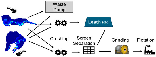
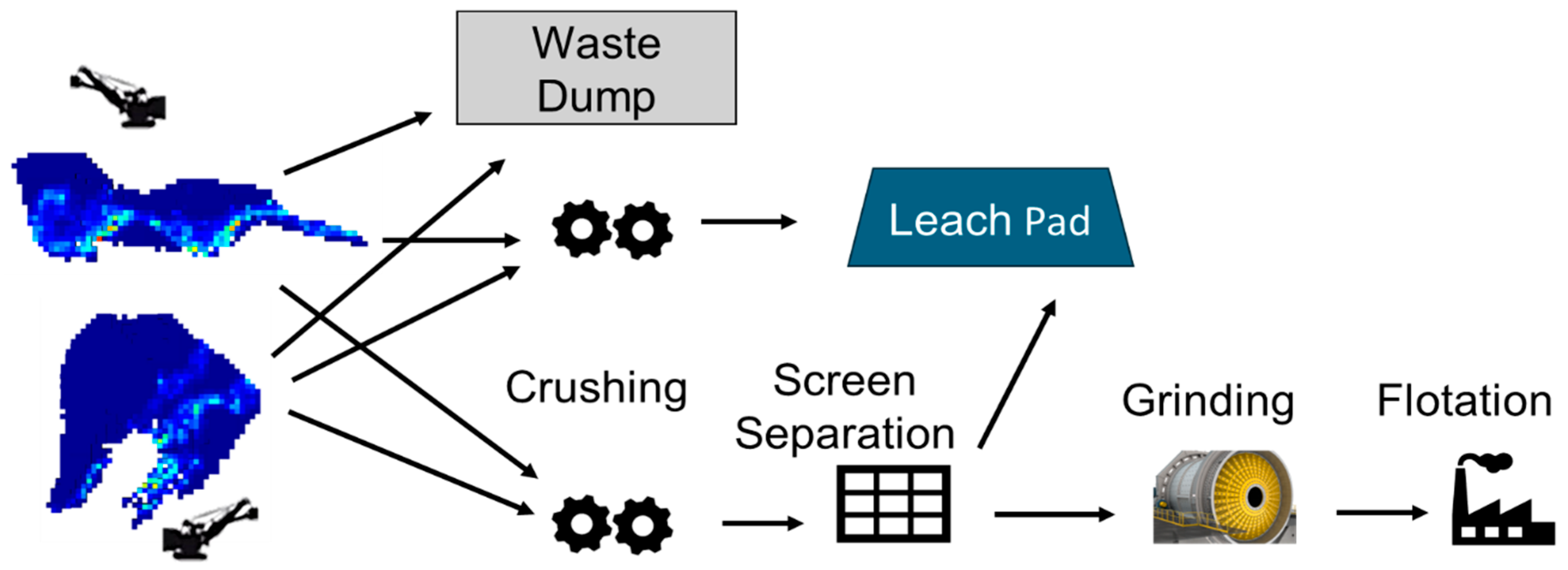
The proposed framework is applied to a gold mining complex to generate an optimized 12-month schedule. The value chain, illustrated in Figure 2, extracts materials from a mineral deposit with two active pit areas using truck and shovel equipment. Materials can be sent to a waste dump, leach pad, or screen separation facility. Materials passing through the screen are sent to the grinding mill and subsequent flotation plant, while oversized materials are diverted to the leach pad. Two operating mode decisions (outlined in Table 4) are considered: the aperture of the screen facility and the grinding mode for the mill. The grinding mode has direct impacts on the capacity and cost per tonne of the mill. The screen setting does not impact cost or capacity but will be considered as conditioning data in the simulation of processing responses.

Figure 2. Gold mining complex and the flow of materials.

Table 4. Impacts of operating modes.

	Screen Separation		Grinding Mill
Operating mode	30 mm	50 mm	Coarse	Fine
Capacity multiplier (%)	100	100	100	90
Processing cost per tonne multiplier (%)	100	100	100	110

Ten geostatistical simulations are used to represent the uncertain properties of the deposit. The two areas have 1421 and 2451 blocks for a total of 3872 blocks. Properties include gold grade, sulfur grade, and hardness measured from blasthole drill penetration rates and simulated for the pit areas to be mined in the future. Hardness values are proportional, giving each block proportions of material that falls into seven bins, as discussed by Both and Dimitrakopoulos [15]. Fifty realizations are used to quantify the processing performance uncertainty. A 12-month schedule will be optimized to demonstrate the proposed method.

3.2. Processing Response Simulations

Three processing responses are simulated for this presented case study: mass passing the screen, gold passing the screen, and gold recovery from flotation. Conditioning data for these simulations are summarized in Table 5 and include the properties of materials being fed to the screen as well as the selected operating modes.

Table 5. Conditioning attributes for simulated processing responses.

	Mass Passing the Screen (%)	Gold Passing the Screen (%)	Gold Recovery (%)
Gold grade before screen (g/t)	Yes	Yes	Yes
Sulfur grade before screen (g/t)	Yes	Yes	Yes
Hardness proportions (%)	Yes	Yes	Yes
Screen aperture (mm)	Yes	Yes	Yes
Grinding mode (fine or coarse)	No	No	Yes
Mass passing the screen (%)	-	Yes	Yes
Gold passing the screen (%)	-	-	Yes

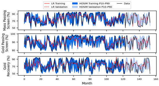
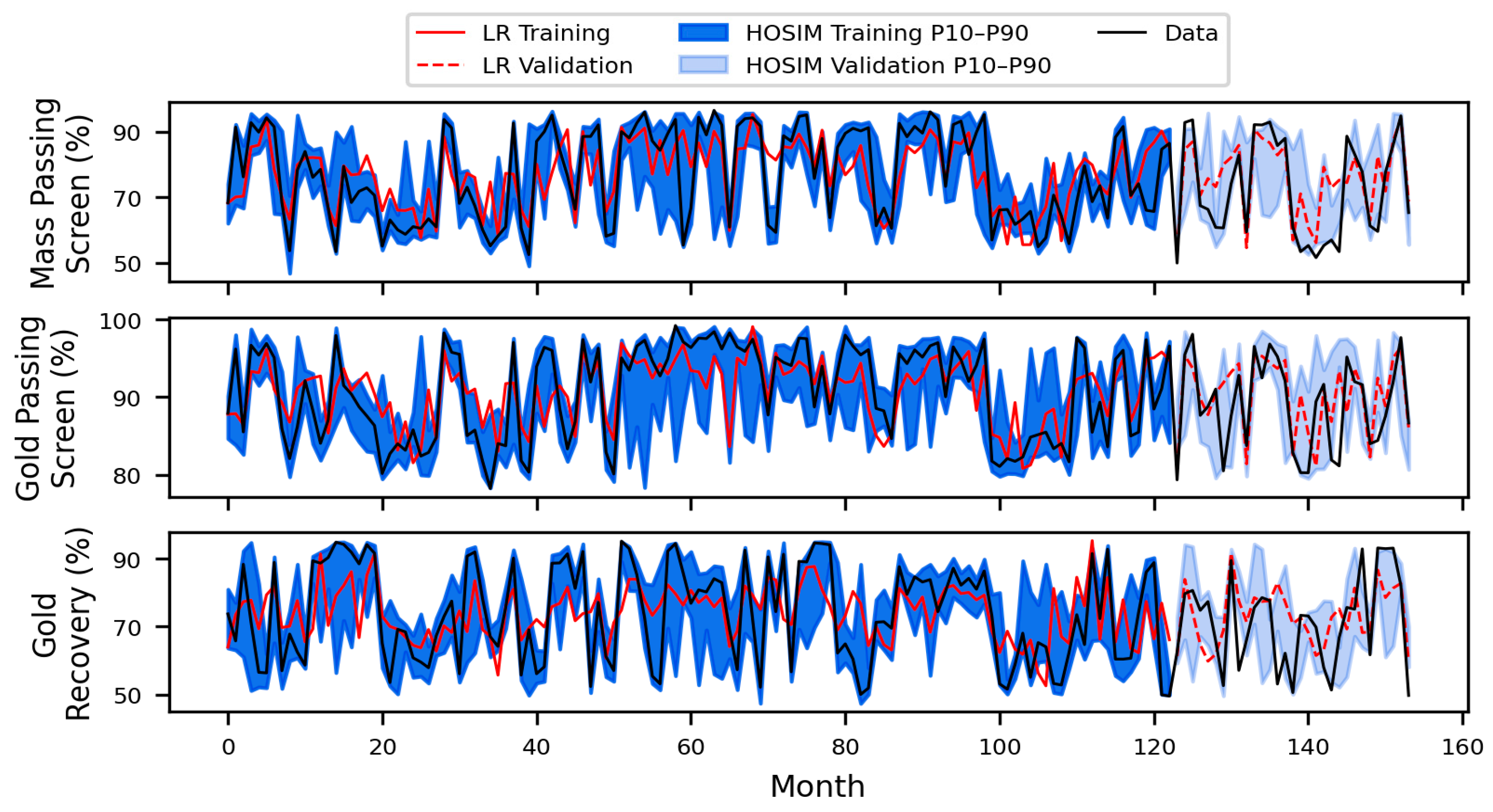
Historical data from 154 monthly periods (a rolling window is used to produce monthly data from original daily data) include material properties being fed to the process circuit and the measured processing responses. The presented high-order simulation (HOSIM) method is compared to a deterministic multi-linear regression model (LR) to illustrate the consequences of ignoring processing response uncertainty. LR is chosen over a more advanced estimator such as a neural network to limit the number of learned parameters and avoid overfitting to the training data. To validate both methods, 120 months of data are included for training, and 34 months are withheld for validation. Figure 3 shows the measured data compared to the LR estimates and HOSIM profile (P10–P90) of 20 realizations for the three processing responses. A visible inspection shows that the simulations cover a wider range of values while LR estimates tend to predict values closer to the mean for each response, matching the expected smoothing effect of regression.

Figure 3. Training and validation of multi-linear regression (LR) and high-order simulation (HOSIM) for processing responses.

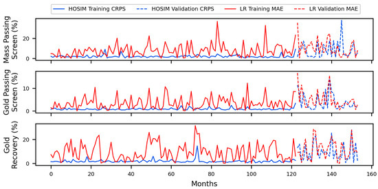
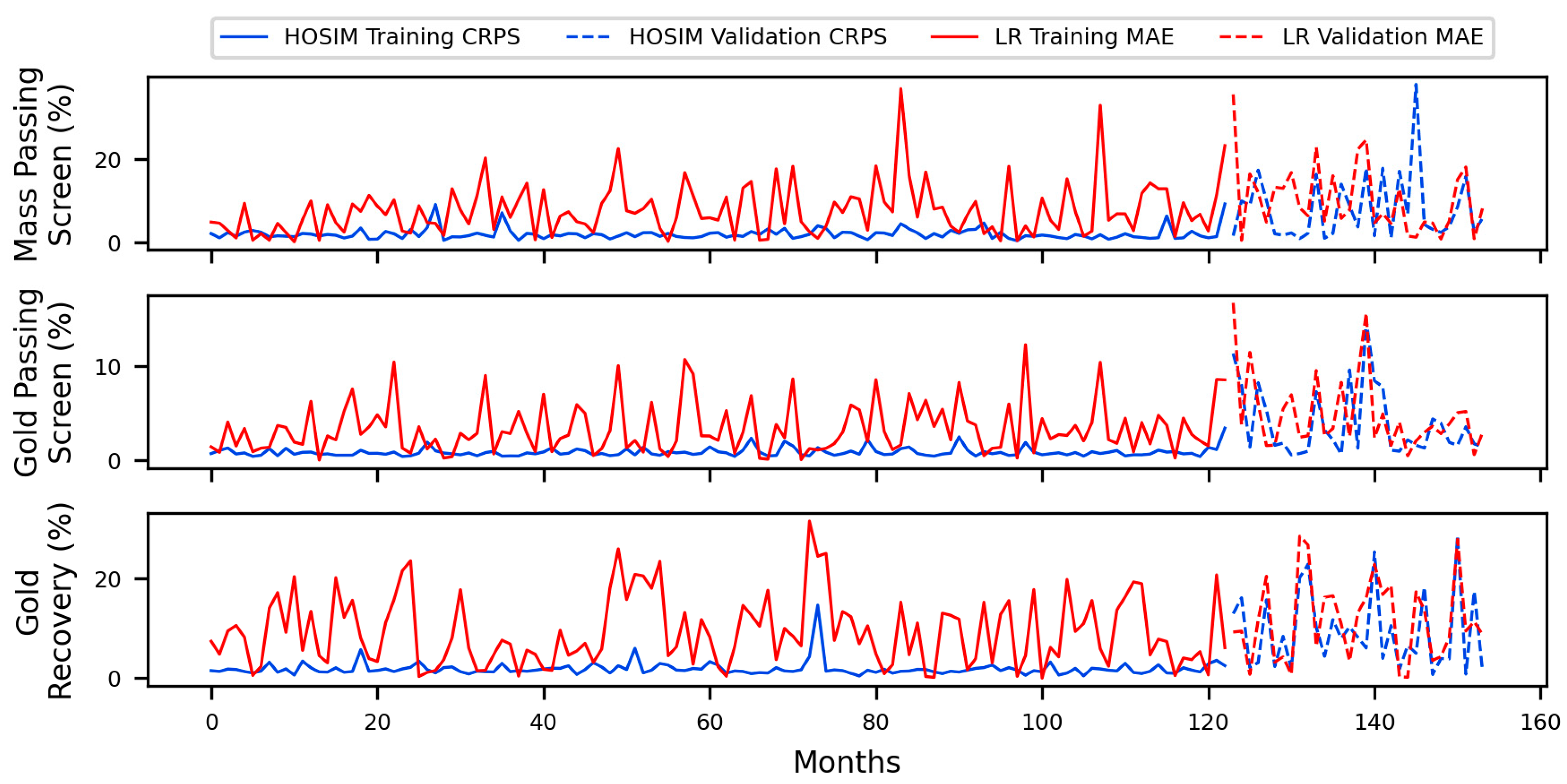
Prediction errors for the simulated values are quantified using continuous ranked probability scores (CRPS) which can be compared directly to mean absolute error (MAE) of the estimated values [35]. These errors are displayed in Figure 4 while average errors over the training and validation datasets are outlined in Table 6. On the training data, the HOSIM prediction errors are consistently lower and more stable than those of the LR estimates. On the validation data, the HOSIM errors are higher and more volatile than the HOSIM training errors, but they are still lower on average than the LR validation errors. These patterns are true for all three processing responses.

Figure 4. Prediction errors for high-order simulation (HOSIM) and multi-linear regression (LR).

Table 6. Average prediction errors for high-order simulation (HOSIM) and multi-linear regression (LR) over the training and validation datasets.

Prediction Set	Mass Passing Screen (%)	Gold Passing Screen (%)	Gold Recovery (%)
LR Training (MAE)	0.08	0.03	0.09
HOSIM Training (CRPS)	0.02	0.01	0.02
LR Validation (MAE)	0.10	0.05	0.12
HOSIM Validation (CRPS)	0.08	0.04	0.09

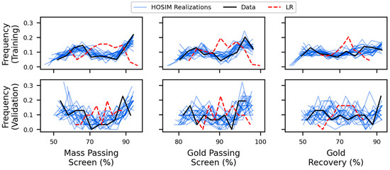
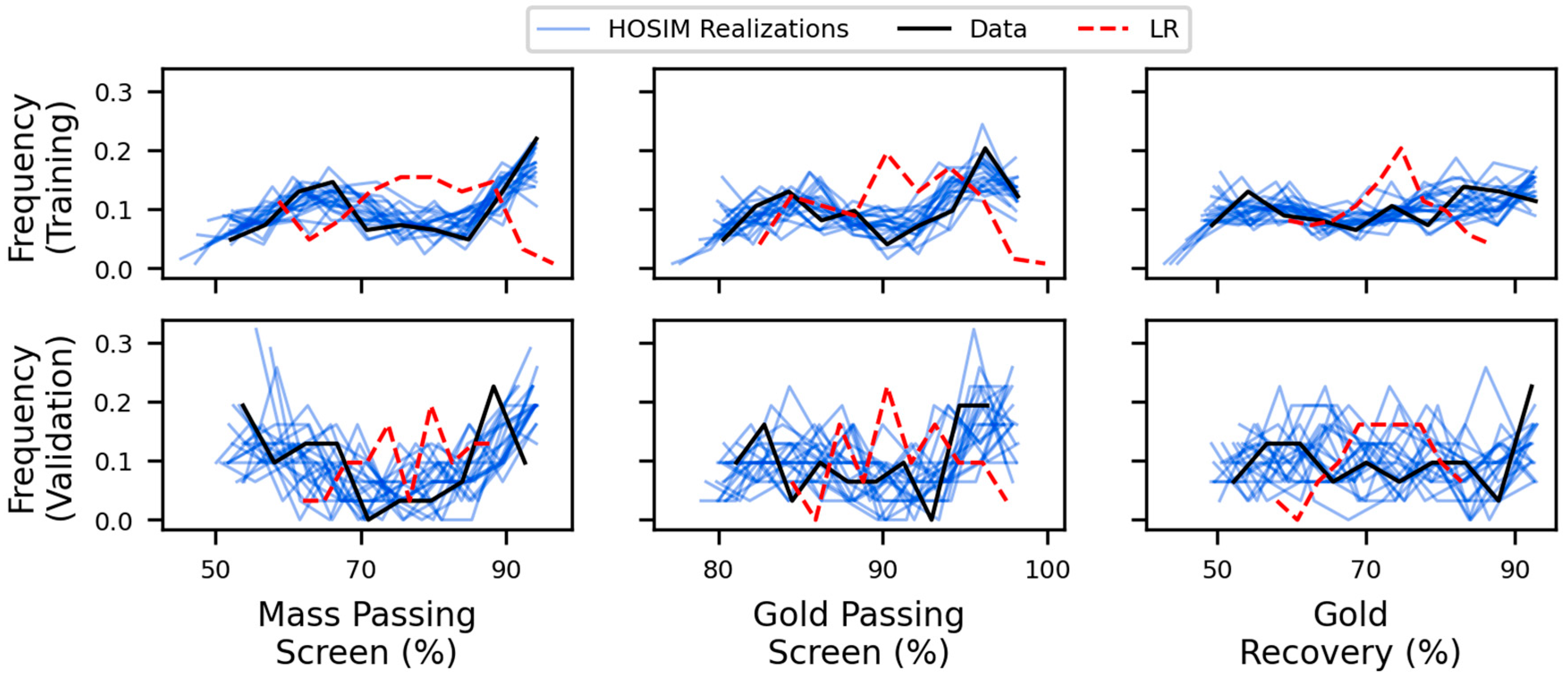
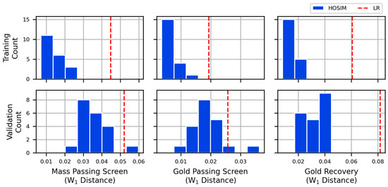
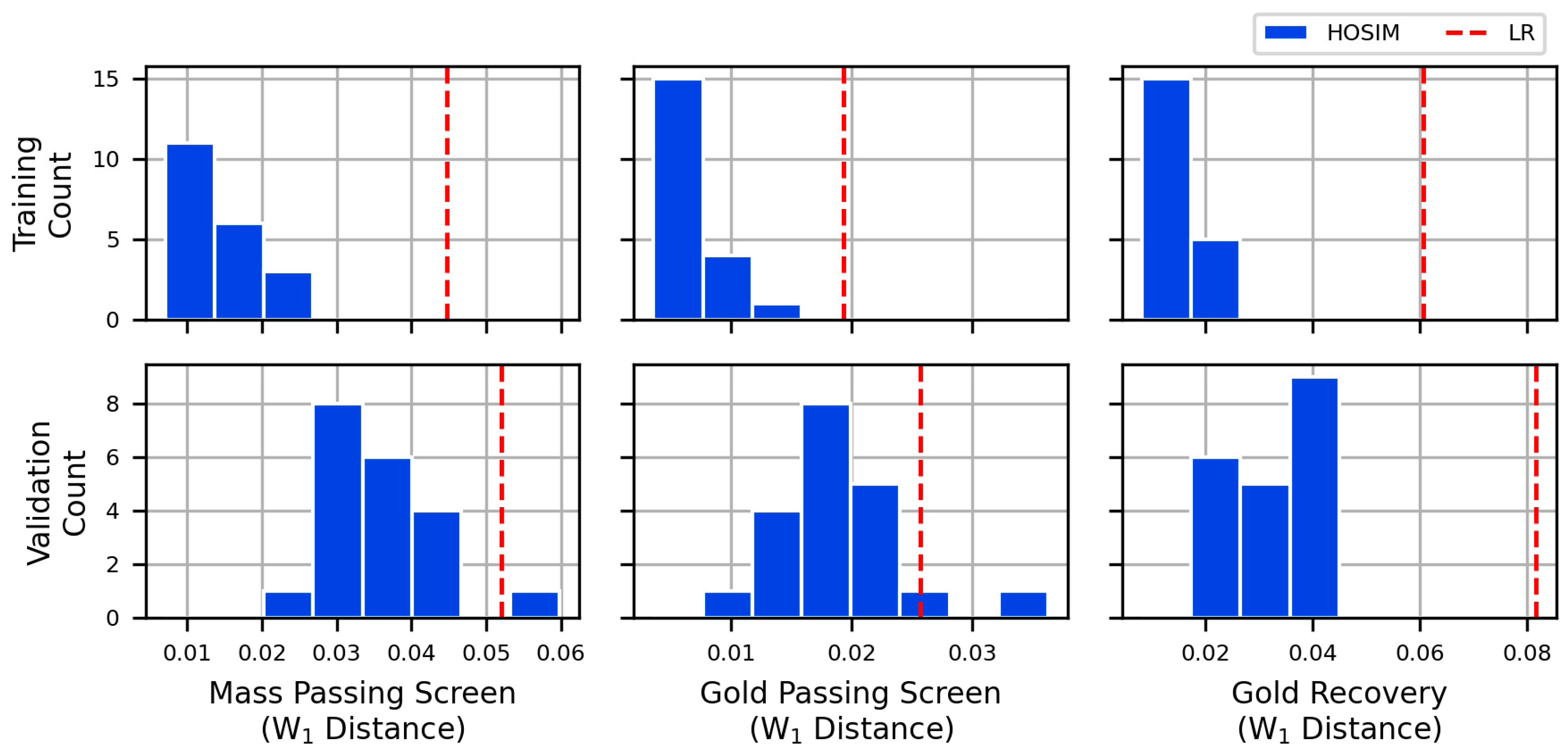
Figure 5 summarizes the data, HOSIM realizations, and LR estimates into histograms. The simulations generally reproduce the data’s distributions, while the regression model shows smoothing with an overrepresentation of medium values for all three responses in both training and validation. The quality of distribution reproduction is quantified using one-dimensional Wasserstein (W₁) distance which measures the difference between two distributions [36]. Figure 6 shows the single W₁ distance between the LR estimates and the data along with a histogram of 20 W₁ distances between the HOSIM realizations and the data, for each response and both datasets. Table 7 shows the LR W₁ distances and the average HOSIM W₁ distances for each response and both datasets. On the training data, the W₁ distances for the HOSIM realizations are categorically lower than those of the LR estimates, showing that the simulations better reproduce the data distributions. The validation results are less pronounced, as only most of the HOSIM realizations have lower W₁ distances than the LR estimates for mass passing and gold passing responses, while the gold recovery response still shows all HOSIM W₁ distances are lower than the corresponding LR W₁ distance.

Figure 5. Histogram comparison of high-order simulations (HOSIM) and multi-linear regression (LR).

Figure 6. Comparison of multi-linear regression (LR) and high-order simulations (HOSIM) in 1-dimensional Wasserstein distance to the data distribution.

Table 7. Average 1-dimensional Wasserstein distances for high-order simulation (HOSIM) and multi-linear regression (LR) over the training and validation datasets.

Prediction Set	Mass Passing Screen (%)	Gold Passing Screen (%)	Gold Recovery (%)
LR Training	0.04	0.02	0.06
HOSIM Training (average)	0.01	0.01	0.01
LR Validation	0.05	0.03	0.08
HOSIM Validation (average)	0.04	0.02	0.03

In summary, the prediction results for HOSIM and LR show that the simulation method produces predictions with lower errors and better distributional reproduction than the regression method. The decrease in simulation quality from training to validation shows the importance of having a sufficient dataset, but the simulations still outperform the regression on all measured indicators. The next section will show how these different prediction models impact mine planning. Note that for all subsequent results, both the HOSIM and LR prediction models are given all 154 samples for training.

3.3. Results

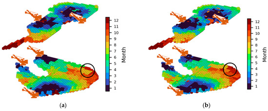
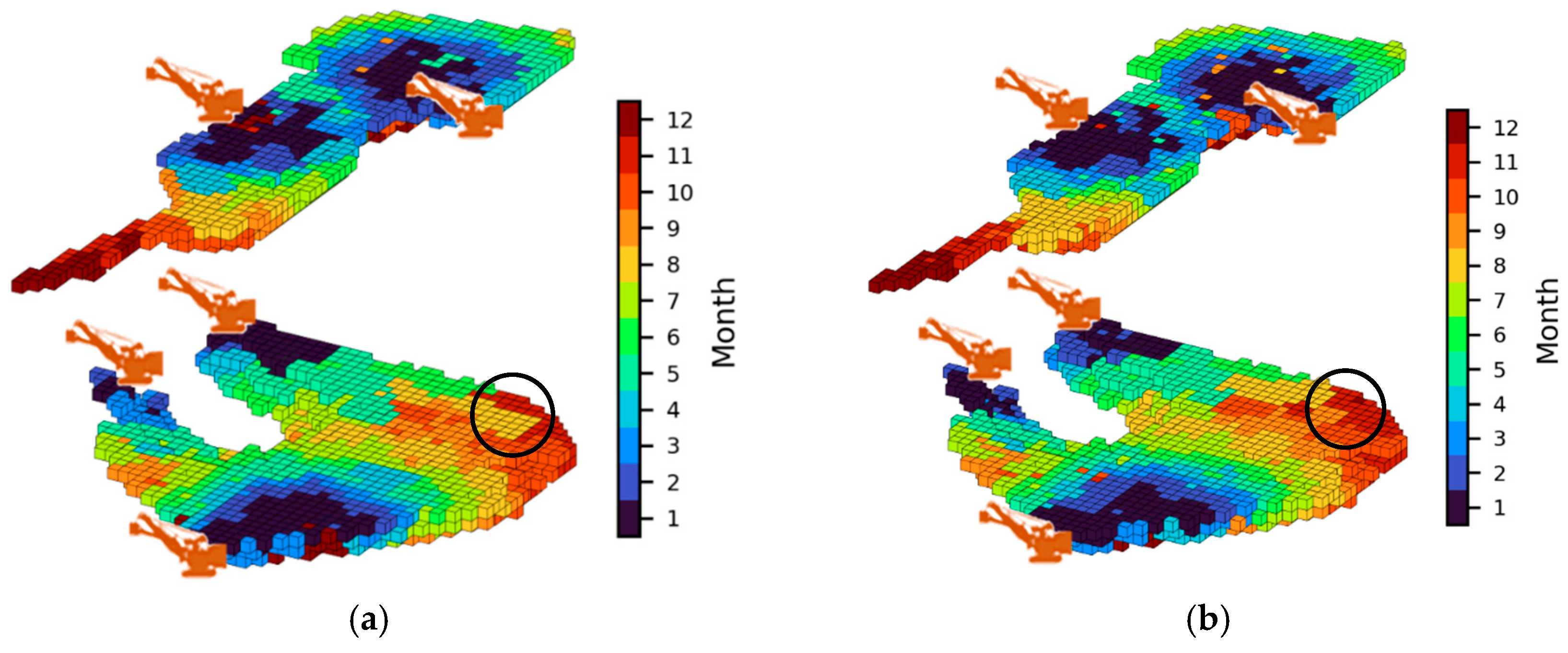
The two prediction methods (HOSIM and LR) shown in the previous section are each used to optimize a production schedule with otherwise identical inputs and settings. The extraction sequences for the two mining areas are shown for both schedules in Figure 7. In both the HOSIM and LR schedules, it is visible that mining begins near the initial locations of the five shovels (shown by the orange shovel icons in Figure 7) and proceeds outward from there. The schedules select slightly different block extraction sequences (with one example circled on the figure), showing that the different processing performance models lead to different mining decisions. The impacts of these differences will be further examined in the subsequent results.

Figure 7. Extraction sequence and initial shovel locations for the HOSIM (a) and LR (b) schedules.

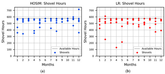
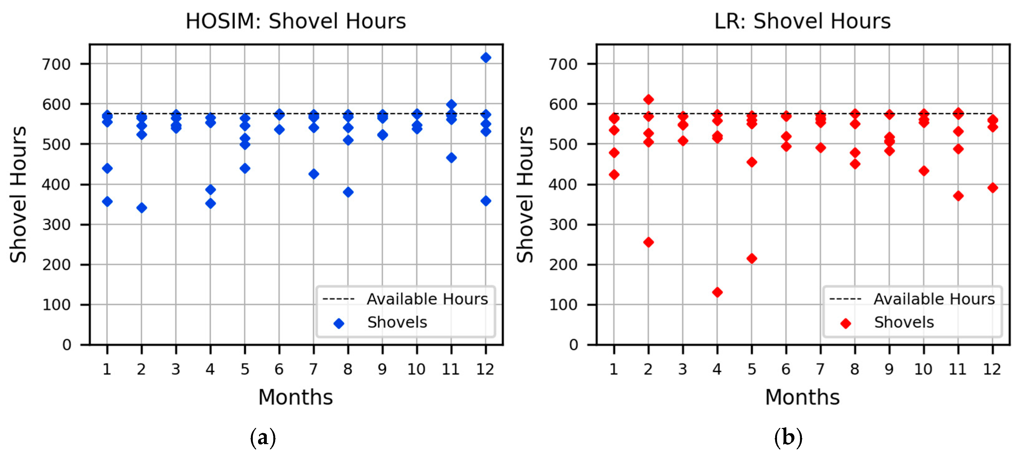
The number of hours scheduled for the five shovels shown in Figure 8 illustrates that both schedules were produced without significant violations over the available hours (576 h each month). Although some minor deviations are present for a small number of shovels, these could likely be addressed by short-term planning which can consider even more detail related to equipment movement.

Figure 8. Shovel hours for the HOSIM (a) and LR (b) schedules.

Table 8 outlines the different operating modes selected by each schedule at the screen and grinding mill. Because these decisions are included as conditioning data for the processing response simulations (along with the material properties), the differences between the two cases lead to different forecasts of downstream performance which are examined through the remaining results.

Table 8. Selected operating modes for both schedules.

Month	HOSIM		LR
	Screen Size (mm)	Grinding Mode	Screen Size (mm)	Grinding Mode
1	30	Coarse	30	Coarse
2	50	Coarse	50	Fine
3	30	Coarse	50	Coarse
4	50	Coarse	50	Coarse
5	50	Fine	30	Fine
6	50	Coarse	50	Fine
7	30	Coarse	50	Fine
8	50	Coarse	50	Fine
9	30	Fine	50	Coarse
10	30	Coarse	50	Fine
11	30	Fine	50	Fine
12	50	Fine	50	Fine

Note: shading is for better readability.

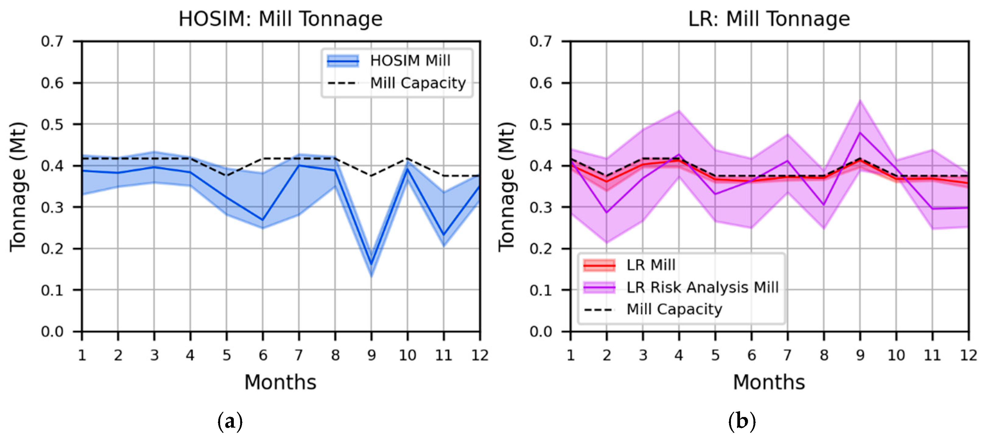
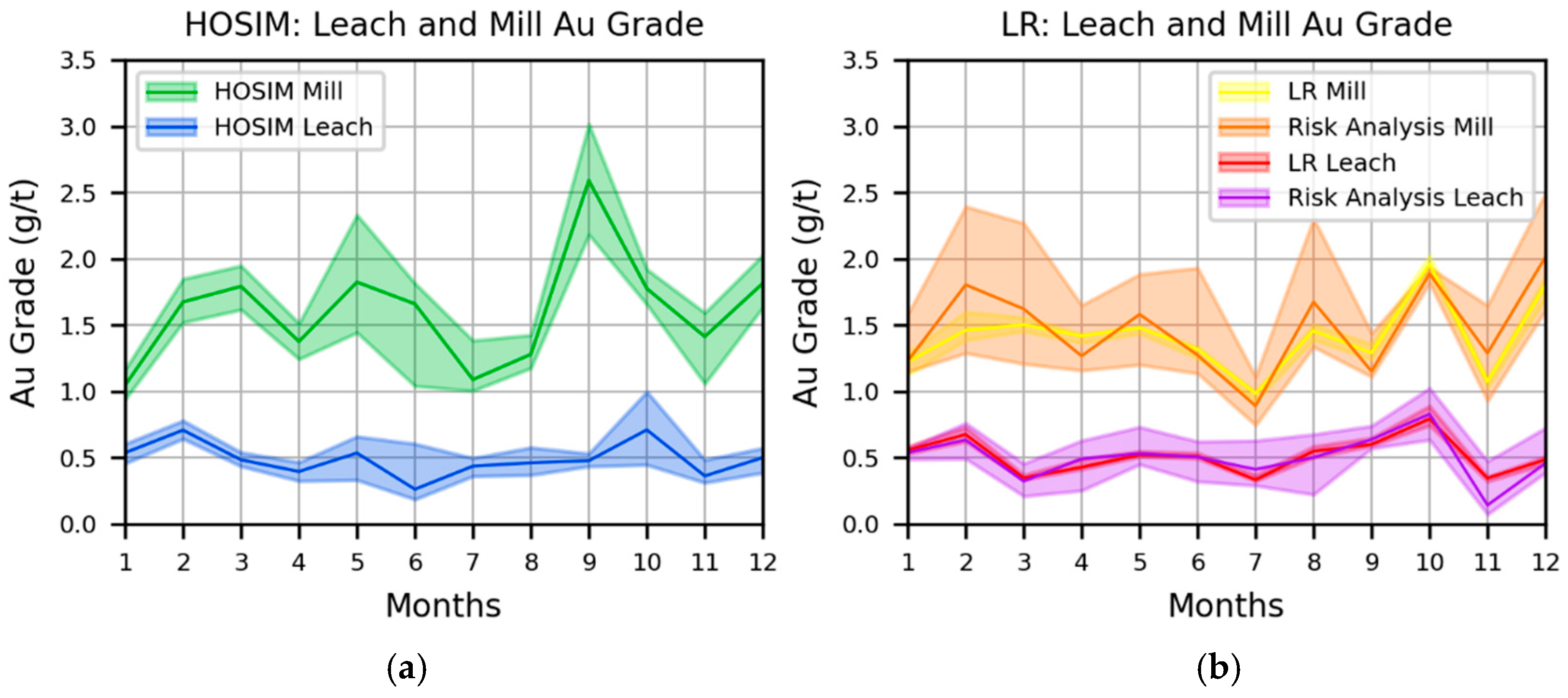
The remaining results use a risk analysis of the LR schedule which is produced by evaluating its decisions using high-order simulations to forecast the processing responses, so it can be compared directly to the HOSIM schedule. For all graphs shown in this section, the shaded regions represent the ranges between 10th and 90th percentiles (P10 and P90, respectively) over the related sets of simulated realizations, and solid lines represent the median (P50) values.

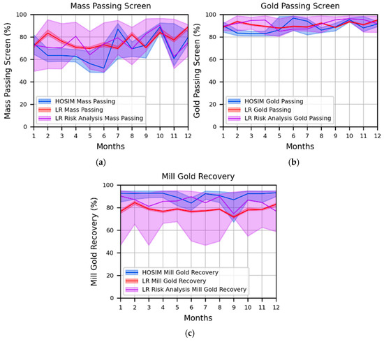
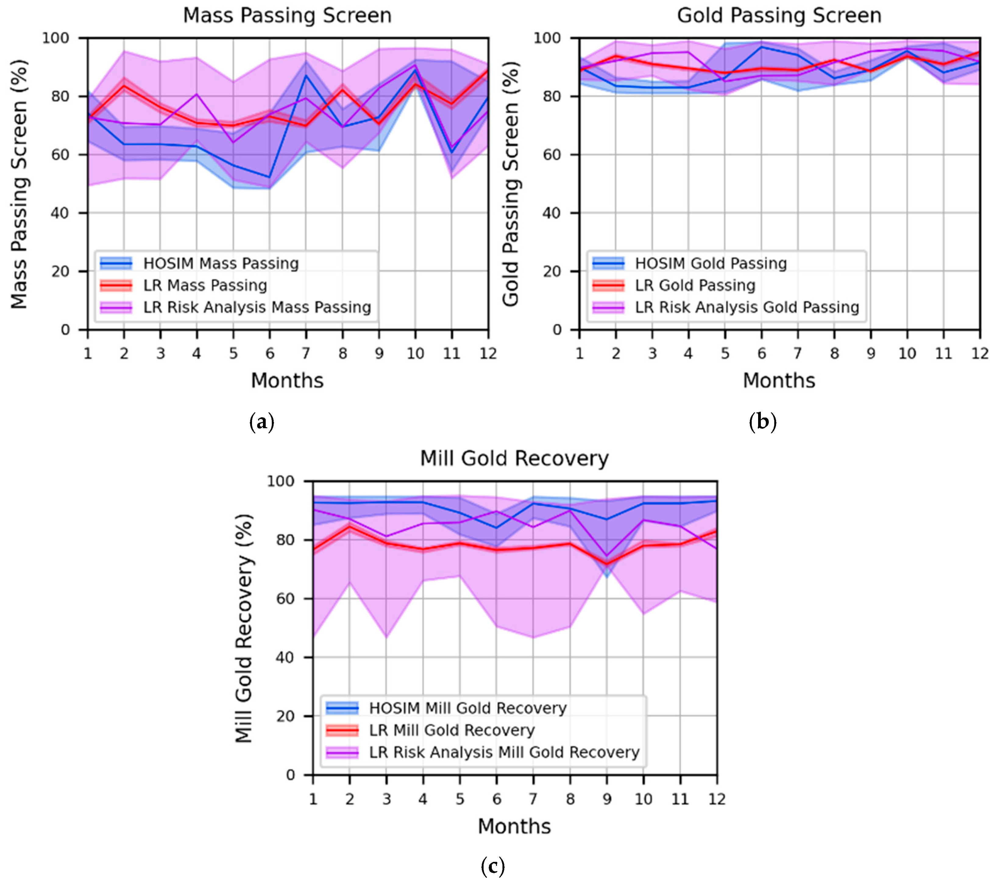
The estimated and simulated processing responses are compared in Figure 9. As expected, the LR model in red underrepresents the variability in these responses and this is highlighted by the risk analysis shown in purple. Beyond this, the most important observation is that the HOSIM schedule was able to make decisions that led to a consistent and high gold recovery at the mill, while the LR risk analysis shows generally lower and much more variable gold recovery.

Figure 9. Comparison and risk analysis of predicted mass passing screen (a), gold passing screen (b), and mill gold recovery (c).

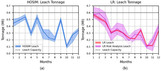
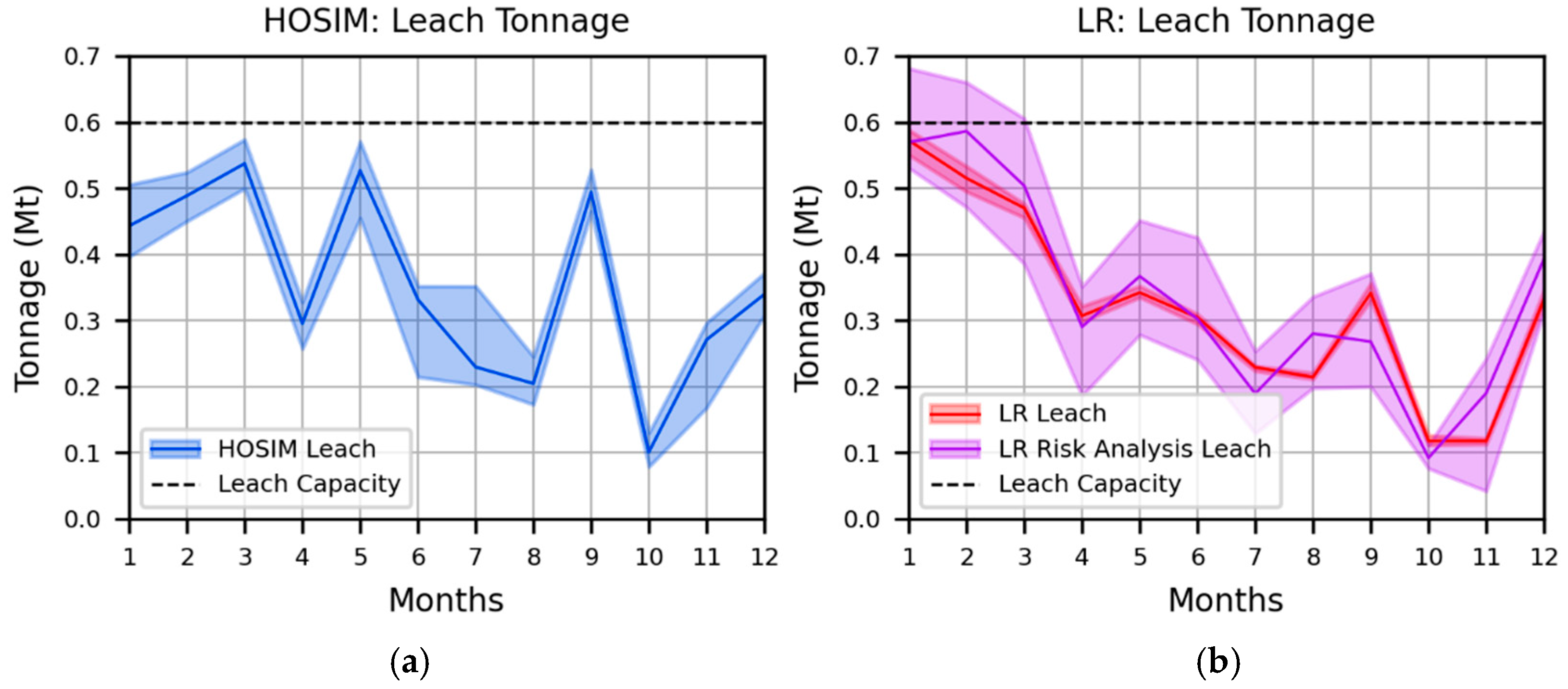
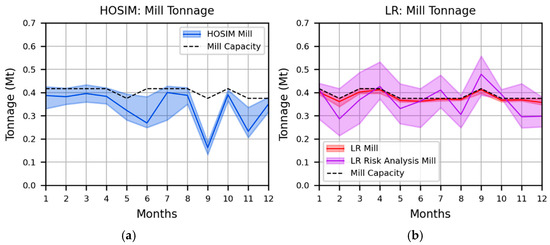
Figure 10 and Figure 11 show the tonnages scheduled to be processed at the leach and mill, respectively. The changing mill capacity lines shown in black are a result of the operating mode decision for the grinding mill, as fine grinding yields a lower throughput. The HOSIM schedule effectively uses the mill capacity and sends other materials to the leach when appropriate. The LR schedule appears to do so based on its own forecast, but the risk analysis reveals that by underestimating the variability of mass passing through the screen, it ends up showing significant risk of going over the processing capacities, particularly at the mill. This effect in part explains why the HOSIM schedule prefers the coarse grinding mode in more periods than the LR schedule does, as the ability to forecast the variability in mill feed leads it to select the higher throughput operating mode.

Figure 10. Comparison and risk analysis of leach tonnage for the HOSIM (a) and LR (b) schedules.

Figure 11. Comparison and risk analysis of mill tonnage for the HOSIM (a) and LR (b) schedules.

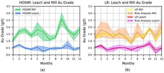
The comparison of gold grades at the leach and mill show in Figure 12 displays another consequence of the LR model underestimating variability. In this case, by using smooth estimates for mass and gold passing the screen, the LR schedule shows a higher variance in feed grades than the LR model predicted, which may cause problems for downstream processing.

Figure 12. Comparison and risk analysis for gold grades at the leach and mill for the HOSIM (a) and LR (b) schedules.

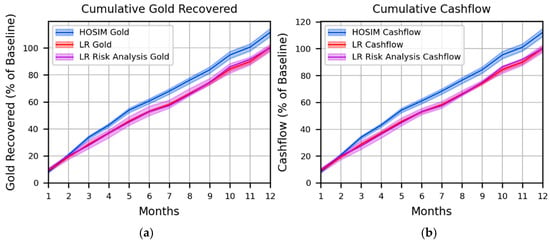
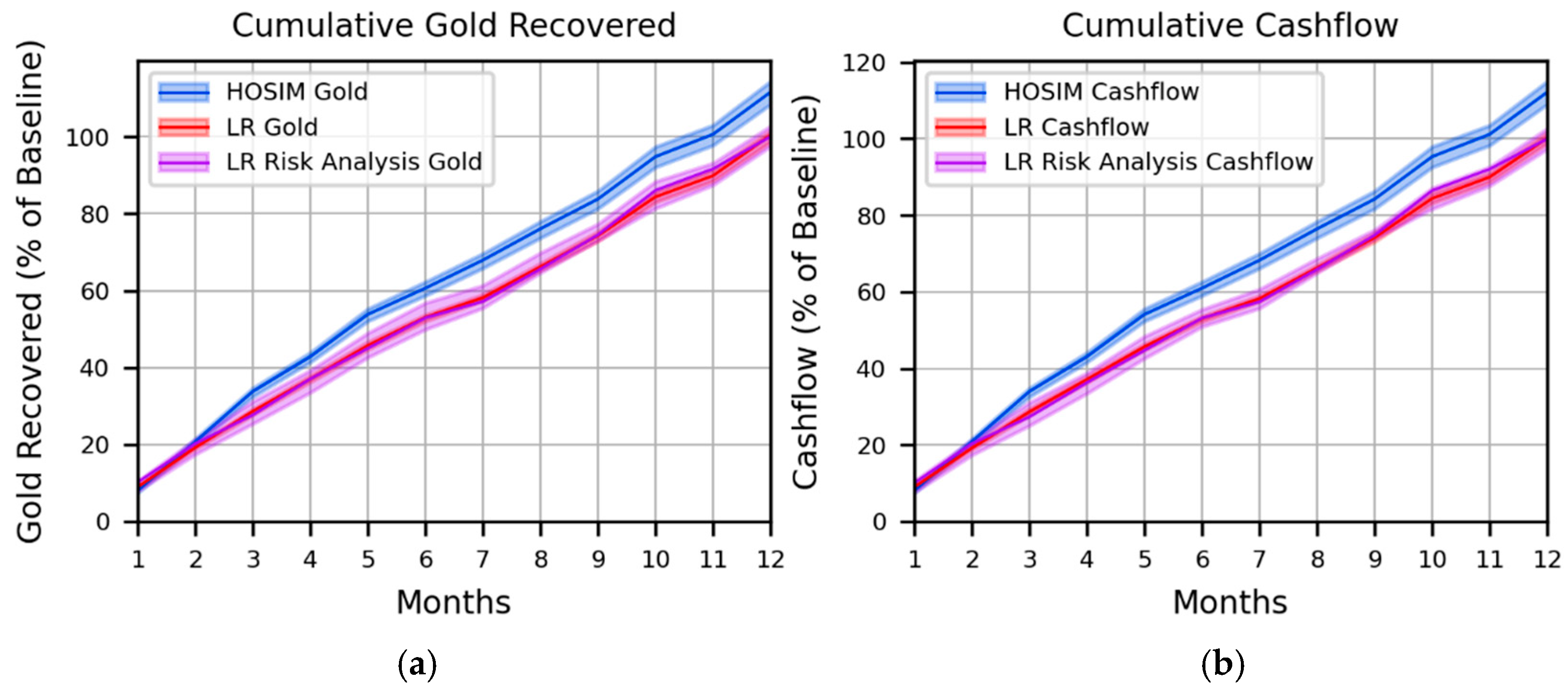
Figure 13 shows the culmination of the mentioned effects in the total gold production and cashflow from the sale of the metal with units scaled to the LR risk analysis baseline for confidentiality. The risk analysis of the LR schedule shows a 0.38% decrease in total gold production and a 0.15% decrease in cumulative cashflow. However, the LR gold production and cashflow forecasts assume that the scheduled materials will be processed despite Figure 9 showing significant risk of violating the mill tonnage capacity. Despite this, the HOSIM schedule, which accounts for processing response uncertainty during the optimization, is still forecasted to produce 11% more gold and 12% more cashflow compared to the LR risk analysis, while also showing less risk of violating the mill capacity. The biggest contributor to this gain is likely the improved gold recovery (Figure 9) found by the HOSIM schedule, and this result quantifies the benefits of incorporating processing uncertainty into decision-making.

Figure 13. Comparison and risk analysis of gold produced and cashflow for the HOSIM (a) and LR (b) schedules.

3.4. Computational Performance

Computational performance of the proposed ML-guided iterated local search (ILS) is compared to a naïve ILS that uses random neighbour ordering to demonstrate the benefit of using online surrogate models to rank and order neighbour solutions during the search. The solvers were tested on the same case study instance as the HOSIM case shown in the previous section and 16 initial solutions were generated for a robust comparison. The computer used was a PC with a 3.6 GHz CPU and 32 GB of memory. For the proposed solver, the measurements include the time required for feature extraction, online model training, and model inference. Note the results focus on optimization run time performance and do not measure the predictive accuracy of the ML models.

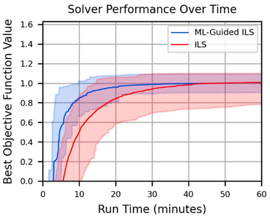
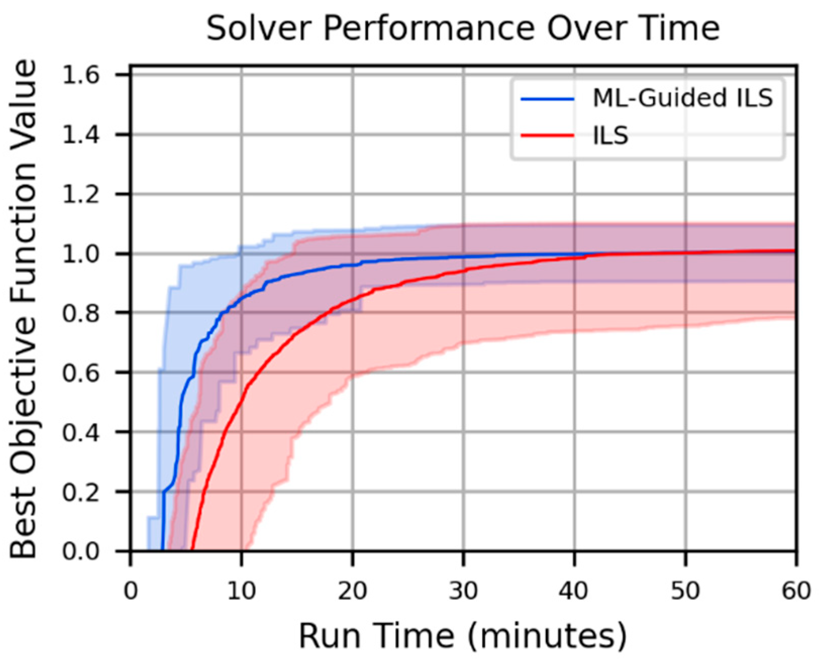
Figure 14 shows the proposed method in blue with the naïve ILS in red. On the graph, solid lines represent the average performance, and shaded areas show the range between minimum and maximum performance over the 16 trials. The results show that the proposed method reaches the same average and best-case objective function values as the naïve ILS, but in less run time, while also improving the worst-case performance.

Figure 14. Solver performance of the proposed method against a simple local search.

Because each of the 16 trials uses the same initial seed solution for both solvers, it is possible to measure how the proposed ML-Guided ILS solver performs against the baseline ILS solver on each trial. Table 9 displays statistics of the 16 differences in objective function values between each solver on the corresponding trials for different time intervals. A positive difference means the proposed method has a greater objective function value. The mean and median values show the proposed solver tends to outperform the baseline in early stages before converging to the same average solution quality. The record of positive, equal, and negative differences shows the same pattern with the proposed method dominating in early stages and becoming roughly even by the 40 min mark. A Wilcoxon signed-rank test [37] is used to measure the statistical significance of the paired objective function value differences. The high W and low $p$-values seen for the 10 and 20 min marks confirm the proposed method has greater objective function values to a statistically significant degree while the later performance differences are statistically insignificant.

Table 9. Statistics and Wilcoxon test results of pairwise objective function value differences between the proposed ML-Guided ILS and baseline ILS.

Run Time (Minutes)	Median	Mean	Minimum	Maximum	Positive–Equal–Negative	W	$\mathit{p}$-Value
10	0.25	0.35	0.00	0.99	15-0-1	135	3.05 $\times$ 10−5
20	0.13	0.12	−0.15	0.37	13-0-3	115	6.55 $\times$ 10−3
40	−0.01	0.01	−0.10	0.20	7-0-9	70	4.70 $\times$ 10−1
60	−0.02	0.00	−0.11	0.17	7-0-9	64	5.90 $\times$ 10−1

4. Conclusions

The present work proposes an optimization framework for monthly production scheduling of mining complexes that enhances two aspects of operational feasibility by incorporating explicit shovel tracking and processing response uncertainty while simultaneously optimizing extraction, destination, downstream flow, and operating mode decisions for a mineral value chain. By explicitly tracking shovel sequences with a nearest neighbour heuristic, the framework produces schedules that more closely align with short-term planning and may reduce the need for major changes to address equipment-related feasibility. By using production data to inform the high-order processing response simulations, forecasts do not rely on any input assumptions, and future measurements can be added to the simulator’s training data to keep it up to date. Results for the gold mining complex demonstrate the benefits of the proposed framework, with realistic extraction sequences and an increase in metal production and cashflow when compared to the schedule made using a deterministic processing response model. Computational results of the solution method show promising improvements by getting good solutions significantly faster than a naïve search method.

Regarding the numbers of stochastic realizations required for the proposed framework, ten was chosen for the material supply uncertainty based on evidence from past studies [3,38] showing that ten for a single deposit is enough to reach solution convergence due to the support effect of the many blocks being scheduled together. However, more testing is needed to prove that this is sufficient in the present application. For the processing response simulations, 50 were used because informal testing showed that using fewer realizations would lead the solver to get stuck in solutions which had lucky simulation results. More rigorous analysis would be needed to find the number that yields general solution convergence.

Future work can extend several areas of this framework. Truck haulage should be included as an additional assessment of operational feasibility. It would also be beneficial to quantify the suboptimality of the greedy heuristic for optimizing shovel sequences. Understanding the impact this has on the overall solutions to the bi-level SIP formulation would help inform potential improvements to the method. More work could also improve the solution method for the upper-level schedule as well. Finally, this work could be integrated with frameworks that connect different planning horizons and use production data to move towards real-time adaptive decision-making for mining complexes.

References

- Pimentel, B.S.; Mateus, G.R.; Almeida, F.A. Mathematical Models for Optimizing the Global Mining Supply Chain. In Intelligent Systems in Operations: Methods, Models and Applications in the Supply Chain; Nag, B., Ed.; IGI Global: Hershey, PA, USA, 2010; pp. 133–163. [Google Scholar]
- Montiel, L.; Dimitrakopoulos, R. Optimizing Mining Complexes with Multiple Processing and Transportation Alternatives: An Uncertainty-Based Approach. Eur. J. Oper. Res. 2015, 247, 166–178. [Google Scholar] [CrossRef] [Scilit]
- Montiel, L.; Dimitrakopoulos, R. A Heuristic Approach for the Stochastic Optimization of Mine Production Schedules. J. Heuristics 2017, 23, 397–415. [Google Scholar] [CrossRef] [Scilit]
- Goodfellow, R.; Dimitrakopoulos, R. Global Optimization of Open Pit Mining Complexes with Uncertainty. Appl. Soft Comput. 2016, 40, 292–304. [Google Scholar] [CrossRef] [Scilit]
- Paithankar, A.; Chatterjee, S.; Goodfellow, R.; Asad, M.W.A. Simultaneous Stochastic Optimization of Production Sequence and Dynamic Cut-off Grades in an Open Pit Mining Operation. Resour. Policy 2020, 66, 101634. [Google Scholar] [CrossRef] [Scilit]
- Dimitrakopoulos, R.; Lamghari, A. Simultaneous Stochastic Optimization of Mining Complexes-Mineral Value Chains: An Overview of Concepts, Examples and Comparisons. Int. J. Min. Reclam. Environ. 2022, 36, 443–460. [Google Scholar] [CrossRef] [Scilit]
- Gershon, M.E. Optimal Mine Production Scheduling: Evaluation of Large Scale Mathematical Programming Approaches. Int. J. Min. Eng. 1983, 1, 315–329. [Google Scholar] [CrossRef] [Scilit]
- Blom, M.; Pearce, A.R.; Stuckey, P.J. Short-Term Planning for Open Pit Mines: A Review. Int. J. Min. Reclam. Environ. 2019, 33, 318–339. [Google Scholar] [CrossRef] [Scilit]
- Both, C.; Dimitrakopoulos, R. Joint Stochastic Short-Term Production Scheduling and Fleet Management Optimization for Mining Complexes. Optim. Eng. 2020, 21, 1717–1743. [Google Scholar] [CrossRef] [Scilit]
- Balboa-Espinoza, V.; Dimitrakopoulos, R. Joint Fleet Management and Stochastic Short-Term Production Planning in Mining Complexes with Carbon Footprint Reduction. Int. J. Min. Reclam. Environ. 2026, 1–22. [Google Scholar] [CrossRef] [Scilit]
- de Carvalho, J.P.; Dimitrakopoulos, R. Integrating Geometallurgy in the Simulation of Processing Plant Responses and Applying Policy Gradient for Shovel Allocation in Operating Mining Complexes. Int. J. Min. Reclam. Environ. 2025, 39, 740–767. [Google Scholar] [CrossRef] [Scilit]
- Hustrulid, W.A.; Kuchta, M.; Martin, R.K. Open Pit Mine Planning and Design, Two Volume Set & CD-ROM Pack, 3rd ed.; CRC Press: London, UK, 2013. [Google Scholar]
- Dimitrakopoulos, R.; Ramazan, S. Uncertainty-Based Production Scheduling in Open Pit Mining. SME Trans. 2004, 316, 106–112. [Google Scholar]
- Matamoros, M.E.V.; Dimitrakopoulos, R. Stochastic Short-Term Mine Production Schedule Accounting for Fleet Allocation, Operational Considerations and Blending Restrictions. Eur. J. Oper. Res. 2016, 255, 911–921. [Google Scholar] [CrossRef] [Scilit]
- Both, C.; Dimitrakopoulos, R. Integrating Geometallurgical Ball Mill Throughput Predictions into Short-Term Stochastic Production Scheduling in Mining Complexes. Int. J. Min. Sci. Technol. 2023, 33, 185–199. [Google Scholar] [CrossRef] [Scilit]
- Coward, S.; Vann, J.; Dunham, S.; Stewart, M. The Primary-Response Framework for Geometallurgical Variables. In Proceedings of the Seventh International Mining Geology Conference, Perth, Australia, 17–19 August 2009; The Australian Institute of Mining and Metallurgy: Melbourne, Australia, 2009; pp. 109–114. [Google Scholar]
- Richmond, A.; Shaw, W. Geometallurgical Modelling-Quo Vadis? In Proceedings of the Seventh International Mining Geology Conference, Perth, Australia, 17–19 August 2009; The Australian Institute of Mining and Metallurgy: Melbourne, Australia, 2009; pp. 115–118. [Google Scholar]
- Coward, S.; Dowd, P.A. Geometallurgical Models for the Quantification of Uncertainty in Mining Project Value Chains. In Proceedings of the International Symposium on the Application of Computers and Operations Research in the Mineral Industry (APCOM), Fairbanks, AL, USA, 23–27 May 2015; Volume 37, pp. 360–369. [Google Scholar]
- Jiang, Y.; Dimitrakopoulos, R. An Application of Simultaneous Stochastic Optimisation on an Open-Pit Copper Mining Complex with Supply, Recovery, and Market Uncertainties. Int. J. Min. Reclam. Environ. 2025, 39, 74–92. [Google Scholar] [CrossRef] [Scilit]
- Mustapha, H.; Dimitrakopoulos, R. High-Order Stochastic Simulation of Complex Spatially Distributed Natural Phenomena. Math. Geosci. 2010, 42, 457–485. [Google Scholar] [CrossRef] [Scilit]
- Yao, L.; Dimitrakopoulos, R.; Gamache, M. A New Computational Model of High-Order Stochastic Simulation Based on Spatial Legendre Moments. Math. Geosci. 2018, 50, 929–960. [Google Scholar] [CrossRef] [Scilit] [PubMed]
- Navarra, A.; Grammatikopoulos, T.; Waters, K. Incorporation of Geometallurgical Modelling into Long-Term Production Planning. Miner. Eng. 2018, 120, 118–126. [Google Scholar] [CrossRef] [Scilit]
- Quelopana, A.; Navarra, A. Incorporating Operational Modes into Long-Term Open-Pit Mine Planning Under Geological Uncertainty: An Optimization Combining Variable Neighborhood Descent with Linear Programming. Min. Metall. Explor. 2024, 41, 2769–2782. [Google Scholar] [CrossRef] [Scilit]
- Nobahar, P.; Xu, C.; Dowd, P. Cost-Integrated AI Meta-Models for Mine-to-Mill Optimisation: Linking Fragmentation, Throughput, and Operating Costs Across the Value Chain. Minerals 2026, 16, 73. [Google Scholar] [CrossRef] [Scilit]
- Lin, J.; Asad, M.W.A.; Topal, E.; Chang, P. Metaheuristic Approaches for Open-Pit Mine Production Scheduling: A Comprehensive Review. Int. J. Min. Reclam. Environ. 2026, 1–33. [Google Scholar] [CrossRef] [Scilit]
- Bengio, Y.; Lodi, A.; Prouvost, A. Machine Learning for Combinatorial Optimization: A Methodological Tour d’horizon. Eur. J. Oper. Res. 2021, 290, 405–421. [Google Scholar] [CrossRef] [Scilit]
- Talbi, E.-G. Machine Learning into Metaheuristics: A Survey and Taxonomy. ACM Comput. Surv. 2022, 54, 129. [Google Scholar] [CrossRef] [Scilit]
- Yaakoubi, Y.; Dimitrakopoulos, R. Decision-Focused Neural Adaptive Search and Diving for Optimizing Mining Complexes. Eur. J. Oper. Res. 2025, 320, 699–719. [Google Scholar] [CrossRef] [Scilit]
- Tenne, Y.; Goh, C.-K. (Eds.) Computational Intelligence in Expensive Optimization Problems; Adaptation Learning and Optimization; Springer: Berlin/Heidelberg, Germany, 2010; Volume 2. [Google Scholar]
- Garrett, C.R.; Kaelbling, L.P.; Lozano-Pérez, T. Learning to Rank for Synthesizing Planning Heuristics. In Proceedings of the Twenty-Fifth International Joint Conference on Artificial Intelligence, New York, NY, USA, 9–15 July 2016; AAAI Press: New York, NY, USA, 2016; pp. 3089–3095. [Google Scholar]
- Chrestien, L.; Edelkamp, S.; Komenda, A.; Pevny, T. Optimize Planning Heuristics to Rank, Not to Estimate Cost-to-Goal. In Proceedings of the Advances in Neural Information Processing Systems; Oh, A., Naumann, T., Globerson, A., Saenko, K., Hardt, M., Levine, S., Eds.; Curran Associates, Inc.: New York, NY, USA, 2023; Volume 36, pp. 25508–25527. [Google Scholar]
- Lourenço, H.R.; Martin, O.C.; Stützle, T. Iterated Local Search. In Handbook of Metaheuristics; Glover, F., Kochenberger, G.A., Eds.; Springer: Boston, MA, USA, 2003; pp. 320–353. [Google Scholar]
- Johnson, M.E. Multivariate Statistical Simulation: A Guide to Selecting and Generating Continuous Multivariate Distributions; Wiley Series in Probability and Mathematical Statistics; Wiley: New York, NY, USA, 1987. [Google Scholar]
- Breiman, L. Random Forests. Mach. Learn. 2001, 45, 5–32. [Google Scholar] [CrossRef] [Scilit]
- Gneiting, T.; Raftery, A.E. Strictly Proper Scoring Rules, Prediction, and Estimation. J. Am. Stat. Assoc. 2007, 102, 359–378. [Google Scholar] [CrossRef] [Scilit]
- Villani, C. Topics in Optimal Transportation; American Mathematical Soc.: Providence, RI, USA, 2021; Volume 58. [Google Scholar]
- Wilcoxon, F. Individual Comparisons by Ranking Methods. Biom. Bull. 1945, 1, 80. [Google Scholar] [CrossRef] [Scilit]
- Albor Consuegra, F.R.; Dimitrakopoulos, R. Stochastic Mine Design Optimisation Based on Simulated Annealing: Pit Limits, Production Schedules, Multiple Orebody Scenarios and Sensitivity Analysis. Min. Technol. 2009, 118, 79–90. [Google Scholar] [CrossRef] [Scilit]
Disclaimer/Publisher’s Note: The statements, opinions and data contained in all publications are solely those of the individual author(s) and contributor(s) and not of MDPI and/or the editor(s). MDPI and/or the editor(s) disclaim responsibility for any injury to people or property resulting from any ideas, methods, instructions or products referred to in the content. |
© 2026 by the authors. Licensee MDPI, Basel, Switzerland. This article is an open access article distributed under the terms and conditions of the Creative Commons Attribution (CC BY) license.