A Novel Spatial–Element Transformer with Dual Attention Architecture for Mineral Prospectivity Mapping

Abstract

In recent years, data-driven mineral prospectivity mapping (MPM) has become a key technical approach for delineating exploration targets. Nevertheless, two major challenges persist. First, sampling is often sparse and irregularly distributed, making it difficult to represent spatial relationships effectively. Second, many existing models implicitly assign equal importance to all geochemical elements. They also fail to jointly model heterogeneous elemental contributions and spatial neighborhood relationships. To address these issues, we propose the Spatial–Element Transformer (SETransformer), which integrates SHapley Additive exPlanations (SHAP)-derived element-importance attention bias with adaptive-bandwidth spatial-decay attention for data-driven MPM. We evaluate the proposed method using data from the Jiama porphyry–skarn Cu-polymetallic deposit in Tibet, China, within two a priori defined metallogenic feature subspaces: Mo-type and Cu-type. SETransformer is benchmarked against conventional machine learning models (Random Forest (RF), eXtreme Gradient Boosting (XGBoost), support vector machine (SVM)), and deep learning baselines (graph convolutional network (GCN) and TabNet). Model performance is assessed under two spatial validation schemes: a south–north hold-out validation and a five-fold spatial block cross-validation. Under both schemes, SETransformer achieves the best overall performance in the two subspaces. The predicted MPMs are consistent with regional geological evidence and exhibit clearer boundaries, providing a useful reference for subsequent target delineation in the study area.

1. Introduction

Mineral resources are strategic and foundational assets for economic development, energy security, and high-technology supply chains. However, China still faces insufficient strategic reserves, limited per capita resource endowment, and increasing external dependence [1]. These challenges make improving mineralization prospectivity prediction a critical task for mineral exploration.

Mineral prospectivity mapping (MPM) is a widely used quantitative approach for integrating geological, geochemical, geophysical, and remote-sensing data to delineate prospective exploration targets [2]. Methodologically, MPM can be classified into three paradigms: knowledge-driven, data-driven, and hybrid approaches [3,4,5]. Knowledge-driven approaches rely on metallogenic theory, expert judgment, and empirical rules, and are suited for data-poor, underexplored regions [6,7,8]. Data-driven approaches extract mineralization patterns from large geoscientific datasets using statistical or machine learning algorithms. They are therefore applicable to well-explored areas with a sufficient number of known deposits [8,9,10]. The limitations of each paradigm have motivated hybrid approaches that combine expert knowledge with data-driven modeling to improve prediction accuracy. Typical hybrid implementations incorporate knowledge-based fuzzy systems or expert-derived weights into data-driven models [11]. This integration helps compensate for the limitations of purely knowledge-driven or purely data-driven paradigms [12,13,14].

Building on the aforementioned MPM paradigms, machine learning techniques have been widely applied in both data-driven and hybrid approaches [15], where they facilitate the modeling of complex nonlinear relationships among geochemical, geophysical, and geological variables [16,17,18,19,20]. Studies have adopted diverse algorithms—including logistic regression [21,22], support vector machines [18,23], artificial neural networks (ANNs) [24], decision trees [25], random forests (RFs) [17,26], and gradient-boosting trees [19]—to build prospectivity models. Despite their success, these methods often struggle with high-dimensional feature spaces, feature selection, and heterogeneous geoscience data. Against this backdrop, deep learning has attracted growing interest for its capacity to learn nonlinear representations from high-dimensional data [27,28]. Architectures explored for MPM include convolutional neural networks, graph neural networks [20], recurrent neural networks [29], long short-term memory networks [30], gated recurrent units [31], deep autoencoders [32], and adversarial networks [33,34,35]. Among CNN-based approaches, architectures such as LeNet [36,37], AlexNet [38], VGGNet [39], GoogLeNet [5], ResNet [40], and U-Net [41] have all been applied.

Transformer architectures, with their self-attention mechanism, offer notable advantages in capturing long-range dependencies and global feature interactions. This capability provides a promising pathway for multi-source, multi-scale geoscience data fusion in MPM. Recent studies have explored various Transformer-based models for mineral prospectivity prediction. For example, ref. [42] applied a deep self-attention model to gold prospectivity, explicitly modeling evidence-layer relationships and spatial heterogeneity, achieving 0.88 accuracy. Ref. [43] combined Transformers with CNNs to overcome CNNs’ limited receptive fields, reaching 0.92 accuracy for Sn–Ag prediction in the Southern Great Xing’an Range. Ref. [44] developed a Transformer–graph convolutional network hybrid (T-GCN) that enhances spatial-structure representation through global self-attention, achieving 97.27% accuracy in the PangXD mining area. Ref. [45] proposed an unsupervised MPM approach based on Vision Transformers, extracting geoscience image features without labels. Finally, ref. [46] introduced a geologically constrained self-supervised Graph-Transformer that leverages graph-based pretraining for spatial coupling and combines it with graph reinforcement learning for adaptive prospectivity optimization. These studies collectively demonstrate the potential of Transformer-based models to improve representation learning and predictive accuracy in MPM.

Although Transformer architectures have achieved remarkable success across a wide range of domains, their application to irregularly sampled geochemical point-cloud data remains constrained by two key challenges. First, most existing CNN- and Transformer-based MPM models rely on regular grids or rasterized inputs, making them ill-suited for sparse and irregularly distributed geochemical sampling locations. Second, geochemical elements are commonly treated as equally weighted features, preventing the simultaneous characterization of heterogeneous elemental contributions and spatial dependencies [47]. To address these limitations, we first define geologically interpretable metallogenic feature subspaces according to the established Jiama metallogenic model and subsequently employ eXtreme Gradient Boosting (XGBoost)–SHapley Additive exPlanations (SHAP) to quantify within-subspace element importance. Building upon this framework, we propose a Spatial–Element Transformer (SETransformer). It integrates SHAP-derived element-importance attention bias with adaptive-bandwidth spatial-decay attention to jointly model elemental associations and spatial context. The proposed model is capable of (i) directly processing discrete sampling points without gridding, (ii) prioritizing diagnostically significant elemental assemblages through attention biasing, and (iii) capturing neighborhood-scale spatial structure that conforms to the distance-decay principle in geostatistics.

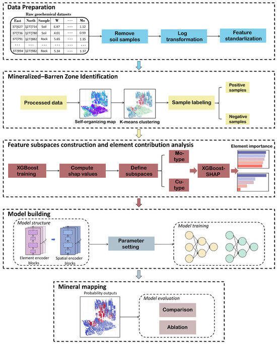
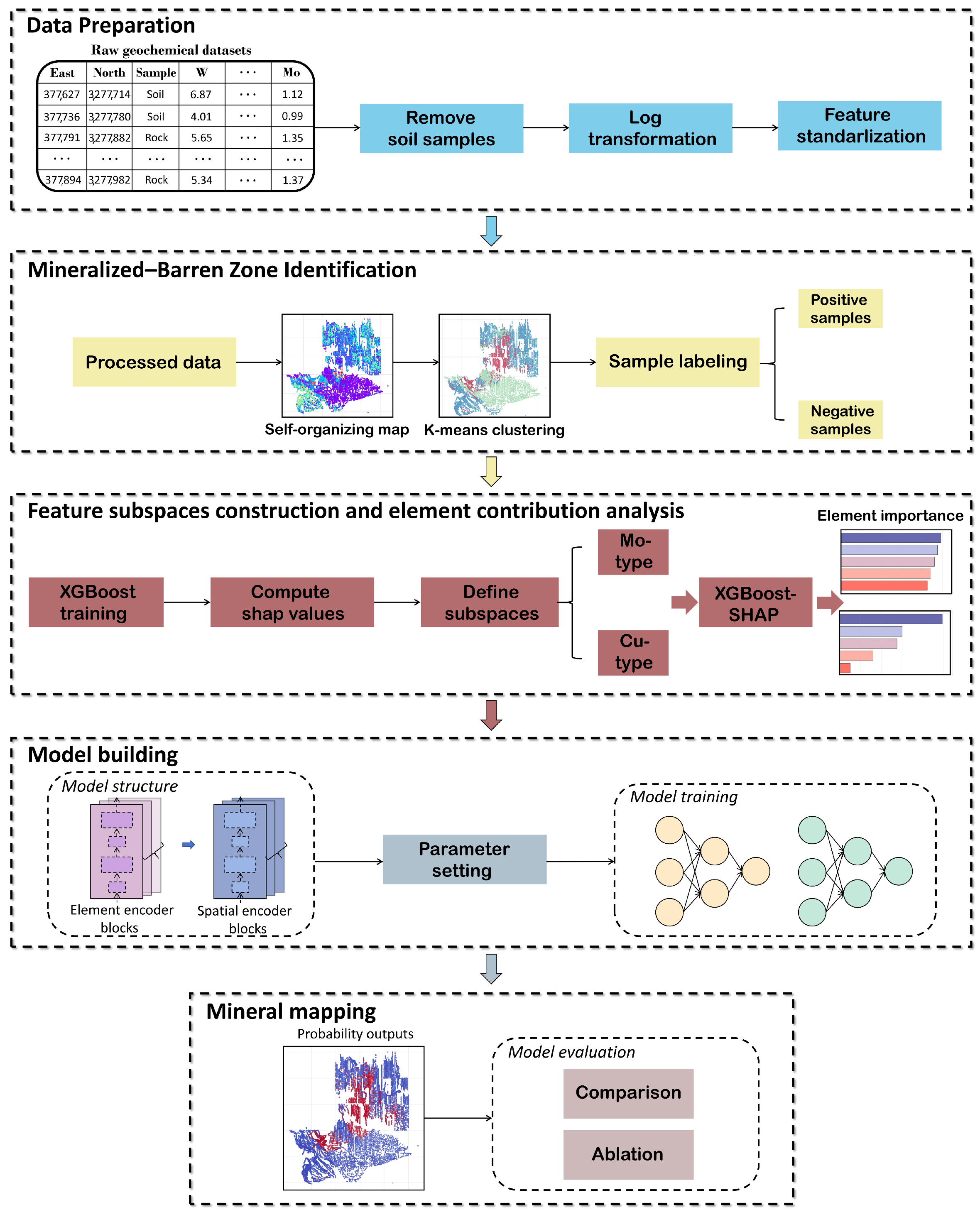
The proposed framework (Figure 1) was evaluated in the Jiama porphyry–skarn Cu-polymetallic deposit. Training samples were first delineated using self-organizing map (SOM)–K-means clustering in conjunction with known mineralization information and regional structural–lithological settings. Subsequently, two metallogenic feature subspaces corresponding to Mo-type and Cu-type mineralization were defined a priori according to the established Jiama metallogenic model. Finally, SETransformer was applied to MPM and compared with a range of conventional machine learning and deep learning models. The results indicate that SETransformer consistently achieves the best overall performance among the evaluated models in terms of average accuracy, precision, F1 score, Cohen’s kappa and Brier score.

Figure 1. Overall workflow of the proposed method.

2. Geological Background

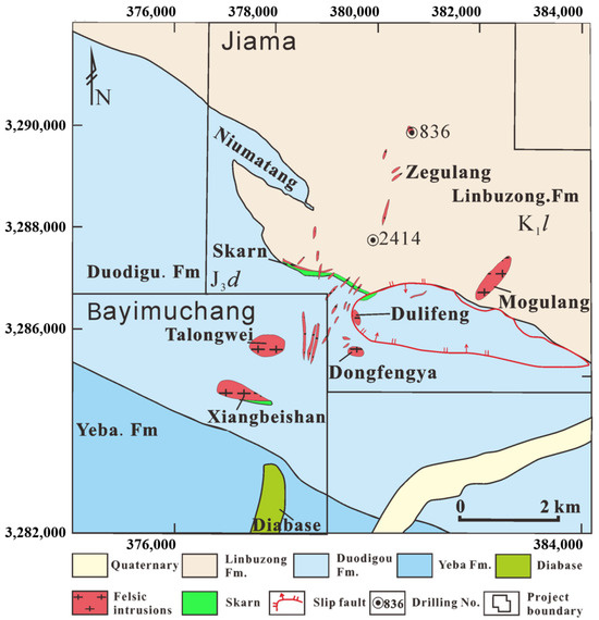
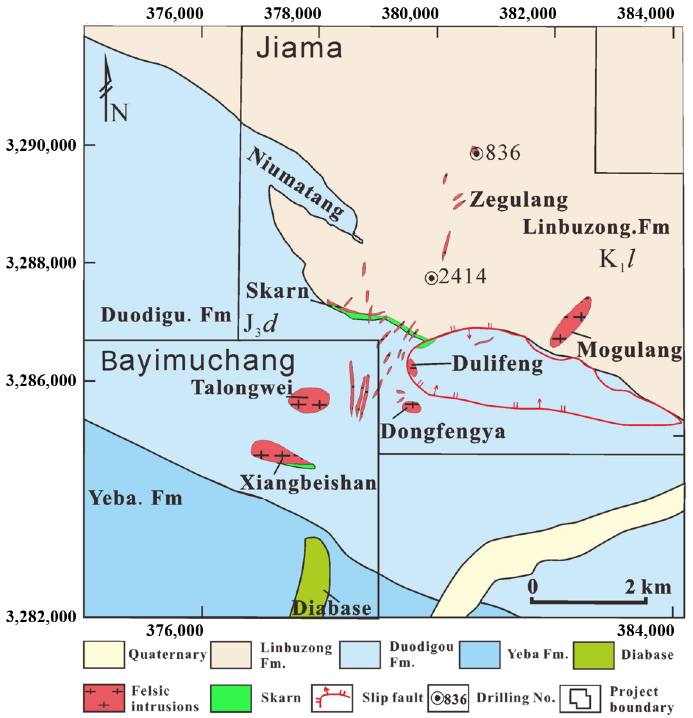
The Jiama deposit is located in the eastern segment of the Gangdese metallogenic belt, along the southern margin of the Lhasa terrane and north of the Yarlung Zangbo suture zone. Exposed strata, listed from older to younger, comprise three principal units: (1) the Upper Jurassic Duodigou Formation (J₃d), interpreted as carbonate deposits of platform-margin bioherm facies and dominated by grayish-white to gray massive crystalline limestone, with minor interbeds of thin-bedded limestone, marlstone, slate, siltstone, and fine sandstone; (2) the Lower Cretaceous Linbuzong Formation (K₁l), the most extensive unit in the mining area, consisting primarily of dark-gray platy siltstone interbedded with grayish-white quartz sandstone and fine sandstone, enriched in carbonaceous material and pyrite, locally containing anthracite seams and coal lines, and conformably overlying the Duodigou Formation; and (3) Quaternary strata, represented by locally distributed slopes and alluvial accumulations in gullies and river valleys (Figure 2). The dominant structural feature is the Jiama–Kajungo thrust system, which forms an imbricate thrust belt from north to south and exerts strong control over the distribution of ore-related intrusions and orebodies in the district [48].

Figure 2. Deposit geology of the Jiama district.

Exploration and previous studies indicate that the Jiama deposit can be subdivided into three main ore segments: the main ore segment, the Nankeng ore segment, and the Zegulangbei ore segment [48]. The main ore segment is located in the central part of the district and comprises the No. I skarn orebody hosted in an interlayer detachment zone, a deep concealed porphyry-type orebody, and an overlying hornfels-type orebody. The No. I orebody trends approximately NW–SE, extends for ∼3000 m, dips to the NE with a down-dip extent of ∼2000 m, and is broadly stratiform to thick-tabular in form, with Pb–Zn mineralization dominating at shallow levels and Cu–Mo at depth. The Nankeng ore segment lies in the southern part of the district and is represented by the No. II skarn orebody [49], which trends NW–SE for ∼1000 m, dips steeply to the NE (commonly $>{50}^{\circ }$), and hosts massive to blocky skarn ores enriched in Cu–Pb–Zn. The Zegulangbei ore segment is located in the northeastern part of the district and remains relatively less constrained by drilling. A thick porphyry-type Mo–Cu orebody has been intersected in drillhole 836, with a thickness of ∼750 m, average Cu grade of ∼0.2%, and average Mo grade of ∼0.03%, indicating promising exploration potential [48].

3. Materials and Methods

3.1. Geochemical Data and Preprocessing

The geochemical dataset used in this study is obtained from 1:10,000-scale rock geochemical surveys conducted by the project team in the mining district. The project covers the major ore-hosting geological units as well as surrounding areas, with a sufficiently high sampling density to delineate multi-element spatial distributions and mineralization-indicator patterns. Samples were collected following a systematic sampling design, labeled, and analyzed by accredited laboratories. In total, 8223 valid geochemical samples were obtained, including concentrations of 39 ore-related and pathfinder elements (e.g., Mo, Cu, W, Bi, Se, Te, and Sn). All elemental concentrations are expressed as mass fractions and reported in parts per million (ppm).

During preprocessing, records containing missing values in any of the 39 elemental variables were removed. This complete-case screening excluded 50 samples, leaving 8173 samples for subsequent analysis. The raw geochemical contents exhibit a typical positively skewed distribution, with values spanning three to four orders of magnitude. This skewness creates two problems: (1) distance-based algorithms such as SOM and K-means are dominated by high-value elements; (2) the large dynamic range impedes model convergence. To address these issues, a base-10 logarithmic transformation was applied. All elemental concentrations in the dataset are strictly positive values above the analytical detection limit; no zero or below-detection-limit values were present, so the logarithm could be applied directly without any substitution or offset. All variables were then standardized to zero mean and unit standard deviation. To prevent information leakage, for the south–north hold-out validation (Section 4.5.1), the scaler was fitted exclusively on the southern training samples and applied unchanged to the northern test samples. For spatial block cross-validation (Section 4.5.2), the scaler was refitted independently using the four training blocks of each fold and then applied to the corresponding held-out block. Following these steps, a multi-element spatial feature database incorporating element concentrations and sampling coordinates was constructed, providing a suitable foundation for subsequent model training and MPM.

3.2. Self-Organizing Map (SOM)

The self-organizing map (SOM) is an unsupervised neural-network method that projects high-dimensional samples onto a low-dimensional grid while approximately preserving their topological relationships. In this study, it is used to represent similarities among multi-element geochemical samples and to facilitate the identification of broad geochemical populations.

Each SOM neuron is associated with a weight vector ${\omega }_i\in {\mathbb{R}}^m$. For an input sample $x\in {\mathbb{R}}^m$, the best matching unit (BMU) is determined as

$$c=arg\underset{i}{min}{∥x-{\omega }_i∥}_2,$$

(1)

where c denotes the index of the neuron whose weight vector is closest to the input sample. During training, the BMU and its neighboring neurons are updated according to

$${\omega }_i(t+1)={\omega }_i\left(t\right)+\eta \left(t\right)h_{ci}\left(t\right)\left[x\left(t\right)-{\omega }_i\left(t\right)\right],$$

(2)

where $\eta \left(t\right)$ is the learning rate and $h_{ci}\left(t\right)$ is the neighborhood function. A Gaussian neighborhood function is adopted:

$$h_{ci}\left(t\right)=exp\left[-{\displaystyle \frac{d_{ci}^2}{2{\sigma }^2\left(t\right)}}\right],$$

(3)

where $d_{ci}$ is the topological distance between neurons c and i, and $\sigma \left(t\right)$ is the neighborhood radius. Both $\eta \left(t\right)$ and $\sigma \left(t\right)$ decrease during training, enabling the SOM to gradually organize samples with similar geochemical characteristics into nearby regions of the map.

In this study, SOM is employed to project multivariate geochemical measurements into a two-dimensional topological space, such that samples with similar element associations are mapped to nearby locations. The resulting low-dimensional representation is both structured and geologically informative, providing an effective basis for subsequent K-means clustering.

3.3. K-Means Clustering Approach

K-means is a classical unsupervised algorithm that partitions a dataset of N samples $\{x_1,x_2,\dots ,x_N\}$ ($x_i\in {\mathbb{R}}^d$) into K disjoint clusters by minimizing intra-cluster variance. Formally, letting $C_k$ denote the set of samples assigned to the k-th cluster with centroid $c_k$, the objective is to minimize the within-cluster sum of squares:

$$J={\displaystyle \sum _{k=1}^K}\sum _{x_i\in C_k}{\parallel x_i-c_k\parallel }^2.$$

(4)

Optimization proceeds by alternating between two steps. First, each sample is assigned to its nearest centroid:

$$d(x_i,c_k)=\parallel x_i-c_k\parallel =\sqrt{\sum _{j=1}^d{(x_{ij}-c_{kj})}^2},$$

(5)

where $x_{ij}$ and $c_{kj}$ denote the j-th component of $x_i$ and $c_k$, respectively. Second, each centroid is updated as the mean of all samples in the cluster:

$$c_k^{(t+1)}={\displaystyle \frac{1}{|C_k|}}\sum _{x_i\in C_k}{x}_i,$$

(6)

where $|C_k|$ denotes the number of samples currently assigned to the k-th cluster. These two steps alternate until convergence.

3.4. SOM–K-Means Joint Clustering Workflow

K-means clusters samples solely based on Euclidean distance, making it sensitive to noise, outliers, and nonlinear structures in high-dimensional geochemical data, which may lead to geologically unstable assignments. To overcome these limitations, we adopted a joint SOM–K-means strategy. SOM first projects multi-element geochemical data onto a two-dimensional topology-preserving manifold, where samples with similar elemental compositions are mapped to neighboring neurons. The resulting SOM neuron weight vectors are then clustered using K-means to obtain the final cluster assignments. This approach reduces noise sensitivity, stabilizes cluster boundaries, and combines SOM’s topological representation with K-means’ efficiency, producing cluster results that are both statistically robust and geologically interpretable.

3.5. SETransformer

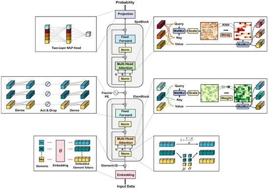
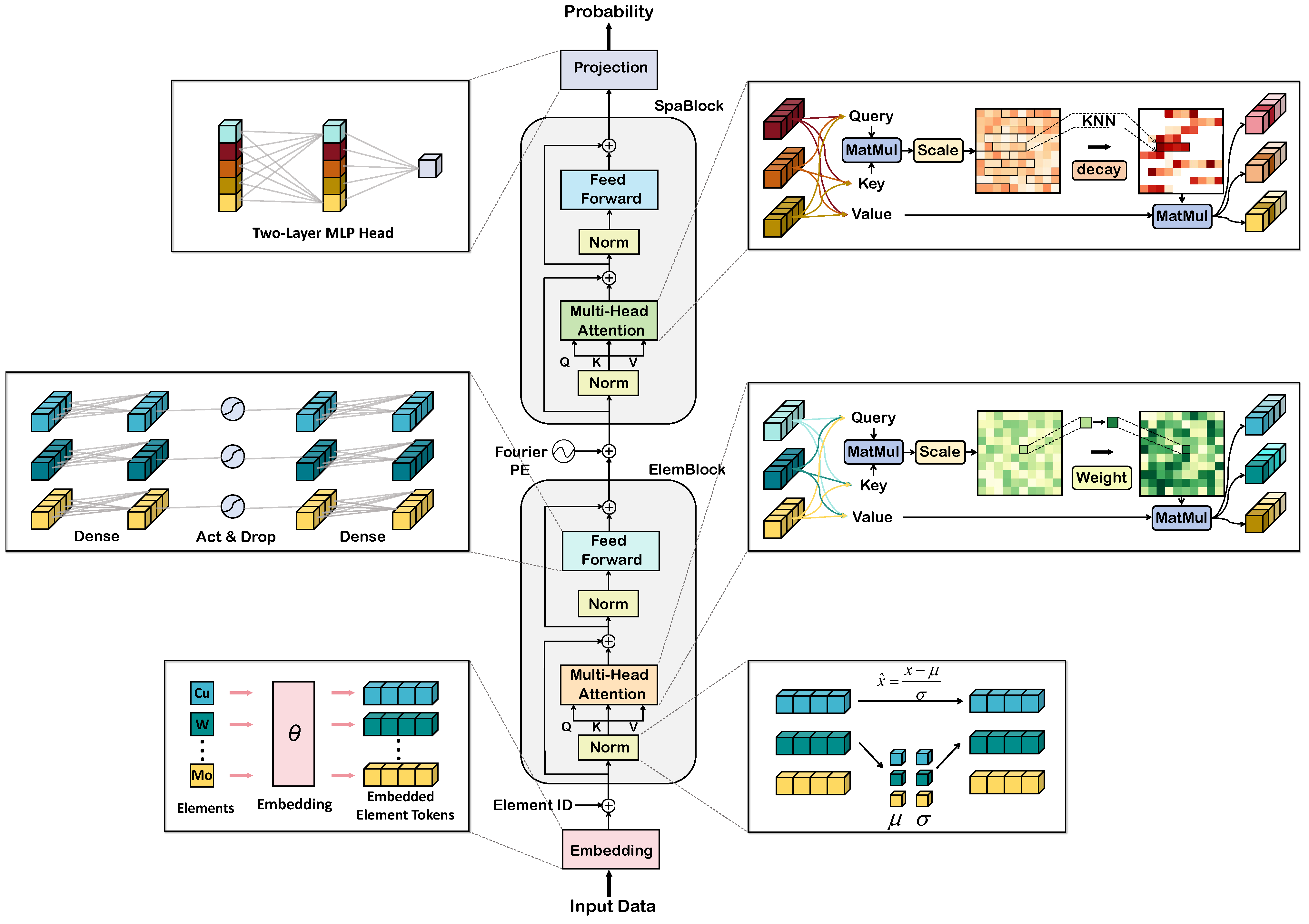
To simultaneously capture complex inter-element coupling in geochemical data and spatial dependency structures under irregular sampling, we designed a dual-encoder architecture. First, the input geochemical element data $X=\{x_1,x_2,\dots ,x_N\}\in {\mathbb{R}}^{N\times m},$ where $x_i\in {\mathbb{R}}^m$ denotes the m-dimensional elemental vector at location i, is embedded via an embedding layer to obtain an element-wise representation $E\in {\mathbb{R}}^{N\times m\times d},$ where d is the embedding dimension (see Equation (7)). The element encoder then processes E to learn interactions among elements and produces a location-wise feature representation $H\in {\mathbb{R}}^{N\times d}.$ Next, the spatial encoder takes H as input and models dependencies among spatial locations, yielding a spatial feature representation $S\in {\mathbb{R}}^{N\times d}$ (Equations (8) and (9)). Finally, a projection module followed by a sigmoid function maps the spatial-encoder output S to the predicted mineralization probability at each location (Equation (10)): $Y=\{y_1,y_2,\dots ,y_N\}\in {\mathbb{R}}^{N\times 1},$ where $y_i$ denotes the predicted mineralization probability at the corresponding geographic location. The overall architecture is illustrated in Figure 3.

$$E=\mathrm{Embedding}\left(X\right),$$

(7)

$$H=\mathrm{ElementEncoder}\left(E\right),$$

(8)

$$S=\mathrm{SpatialEncoder}\left(H\right),$$

(9)

$$Y=\sigma \left(\mathrm{Projection}\left(S\right)\right).$$

(10)

Figure 3. Framework of the proposed SETransformer, consisting of an element encoder and a spatial encoder.

3.5.1. Spatial and Element Encoder Stacks

Prior to the element encoder, the geochemical element values at each location are transformed into m per-element tokens. Specifically, each scalar element concentration is mapped to a d-dimensional embedding through a shared two-layer projection network, and a learnable element-identity embedding is then added to each token to explicitly indicate its corresponding geochemical element. This yields m element tokens per location, which form the input sequence to the element encoder.

The element encoder is composed of a stack of Pre-Layer Normalization (Pre-LN) Transformer blocks, each of which includes a multi-head self-attention (MHSA) sublayer and a feed-forward network (FFN) sublayer. The MHSA module captures global inter-element dependencies, whereas the FFN further learns higher-order compositional patterns across elements. To explicitly emphasize heterogeneity in metallogenic relevance across elements, we incorporate an element-importance attention bias into the self-attention module, thereby enhancing the model’s sensitivity to key ore-forming element associations. In each sublayer, inputs are normalized using Pre-LN, and residual connections are applied to combine sublayer outputs with their inputs, improving training stability. Through hierarchical processing across multiple element-encoder layers, the model learns metallogenic associations among elements. Finally, the m contextualized element tokens at each location are aggregated by mean-pooling to produce a single location-wise element-feature representation $H\in {\mathbb{R}}^{N\times d}$.

The spatial encoder is designed to model spatial dependencies in geochemical observations. Specifically, the output of the element encoder is added to the corresponding Fourier positional encoding to obtain a joint representation that contains both elemental information and location information. These representations are then fed into a network consisting of multiple Pre-LN Transformer blocks to capture structural relationships among sampling locations. Similar to the element encoder, this encoder contains MHSA and FFN sublayers; however, its attention weights are driven by relationships among locations. To strengthen locality awareness and suppress noise, we introduce adaptive-bandwidth spatial-decay attention that assigns lower weights to distant locations, encouraging the model to focus on geologically coherent local structures. After this stage, the model obtains an integrated representation that jointly reflects element-level and spatial dependencies.

3.5.2. SETransformer Components

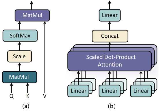
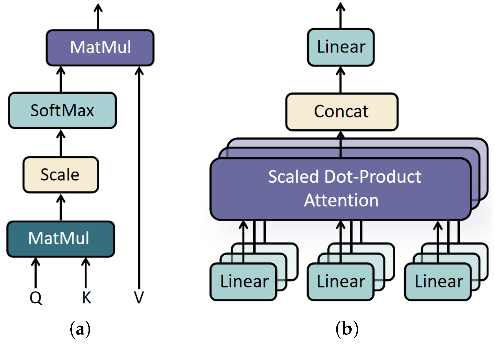
Self-attention. We build on the standard scaled dot-product self-attention [50] (Figure 4a). Given an input sequence $X=[x_1,\dots ,x_n]$ with $x_i\in {\mathbb{R}}^{d_{\mathrm{model}}}$, three linear projections produce queries, keys, and values $Q=X{W}_Q$, $K=X{W}_K$, $V=X{W}_V$, and the attention output is

$$\mathrm{Attention}(Q,K,V)=\mathrm{softmax}\left({\displaystyle \frac{Q{K}^{\top }}{\sqrt{d_k}}}\right)V$$

(11)

where $d_k$ is the per-head dimension. Multi-head self-attention (MHSA) (Figure 4b) runs h such attention functions in parallel over different projection subspaces and concatenates their outputs, enabling the model to capture feature relationships at multiple scales. These standard operations serve as the backbone into which we introduce the two domain-specific mechanisms described below.

Figure 4. Standard attention operations used in SETransformer: (a) scaled dot-product attention and (b) multi-head attention, in which parallel attention heads are concatenated and linearly projected.

Pre-layer normalization. To stabilize the training of the deep encoder stacks, we adopt the Pre-LN configuration [51,52], in which normalization is applied to the sublayer input,

$$y=x+\mathrm{SubLayer}\left(LayerNorm\right(x\left)\right).$$

(12)

Compared with Post-LN, the residual path preserves the unnormalized input and allows gradients to propagate more smoothly through deep networks, improving convergence stability.

Feed-forward network. Each Transformer block includes a position-wise FFN that applies the same nonlinear transformation independently to every element token and every location-wise feature vector. It consists of two linear layers with a GELU activation:

$$\mathrm{FFN}\left(x\right)=\varphi (x{W}_1+b_1)W_2+b_2,$$

(13)

where the intermediate dimension $d_g$ expands the representation capacity.

Element-importance attention bias. In the element encoder, we augment the pre-softmax self-attention scores with a bias term derived from element importance. To quantify how element importance affects inter-element attention, we define an element-importance attention bias as

$${\mathrm{bias}}_{ij}=\lambda ·(g_i+g_j),$$

(14)

where i and j index the elements, $g_i$ and $g_j$ denote their respective SHAP-derived element weights, and $\lambda$ controls the strength of the prior bias.

This mechanism assigns each element an importance weight that directly influences inter-element interactions in the self-attention module. By explicitly amplifying the attention contributions of high-importance elements, the model is guided to focus on more diagnostically informative element assemblages, thereby improving predictive accuracy.

Adaptive-bandwidth spatial-decay attention. To enhance the spatial encoder’s ability to model local spatial structure, an adaptive-bandwidth spatial-decay attention strategy is introduced that combines a K-nearest neighbor (KNN) mask with a spatial-decay factor. This design encourages attention to concentrate on geochemical relationships among nearby sampling locations while suppressing spurious associations between distant locations, thereby improving the spatial resolution of prospectivity prediction.

Concretely, prior to computing spatial self-attention scores, KNN is used to construct a spatial mask matrix and a distance-decay factor for each location. First, we compute pairwise Euclidean distances $d_{ij}$ between all locations in the current graph to quantify the spatial proximity between sampling locations i and j. For each sample i, we then select its K nearest neighbors to define its local neighborhood, and build a binary KNN mask matrix M:

$${\mathrm{M}}_{ij}=\left\{\begin{array}{cc}1,\hfill & \mathrm{if}j\mathrm{is}\mathrm{one}\mathrm{of}\mathrm{the}K\mathrm{nearest}\mathrm{neighbors}\mathrm{of}i,\hfill \\ 0,\hfill & \mathrm{otherwise}.\hfill \end{array}\right.$$

(15)

After neighborhood determination, the contribution of each neighboring location is modulated by the following distance-decay factor:

$${\mathrm{decay}}_{ij}=exp\left(-{\displaystyle \frac{d_{ij}^2}{{\sigma }^2}}\right),$$

(16)

where $\sigma$ is an adaptive bandwidth controlling how rapidly attention weights decay with increasing distance. Rather than treating $\sigma$ as a fixed hyperparameter, we estimate it from the data as the median of the genuine KNN neighbor distances within the training graph. This makes the decay kernel adaptive with respect to coordinate scaling and local point density. Locations that are closer receive larger decay factors and thus contribute more to attention, whereas more distant locations receive smaller decay factors. We combine the mask and the decay factor into a non-negative spatial kernel:

$$G_{ij}=M_{ij}·{\mathrm{decay}}_{ij},$$

(17)

where $G_{ij}=0$ outside the local neighborhood. Instead of adding G directly to the attention logits, we inject it as an additive log-bias on the pre-softmax scores, which is equivalent to multiplicatively reweighting the attention probabilities by G while masking out positions with $G_{ij}=0$:

$$\begin{array}{c}\hfill A_{ij}={\mathrm{softmax}}_j\left({\displaystyle \frac{q_i^{\top }{k}_j}{\sqrt{d_k}}}+log{G}_{ij}\right),\\ \hfill \mathrm{where}log{G}_{ij}\to -\infty \mathrm{when}{G}_{ij}=0.\end{array}$$

(18)

Compared with directly scaling the logits by G, this log-bias formulation yields cleaner gradients and a well-defined hard mask at $G_{ij}=0$. This combined design confines attention to local neighborhoods and applies distance-dependent weighting, suppressing long-range noise while emphasizing geologically coherent local structures. Critically, during training, the neighborhoods are built solely among the training locations; when the trained model is applied to the test set, the neighborhoods are built solely among the test locations.

Fourier positional encoding. Fourier positional encoding maps raw two-dimensional geographic coordinates into a higher-dimensional feature space, enabling the model to capture spatial dependencies at multiple scales. By projecting coordinates onto sinusoidal functions of exponentially spaced frequencies, the encoder obtains periodic, hierarchical spatial representations that support learning of both local and global spatial structure. Let the normalized spatial coordinate of each sample be

$$p=(p_{\mathrm{east}},p_{\mathrm{north}})\in {[0,1]}^2,$$

(19)

where $p_{\mathrm{east}}$ and $p_{\mathrm{north}}$ are the coordinate values along the easting and northing axes, respectively. Define a set of B exponentially spaced frequencies $f=[2^0,2^1,\dots ,2^{B-1}]$, where B is the number of frequency bands. Each coordinate axis is independently projected onto every frequency to obtain a phase value:

$${\varphi }_{d,k}=2\pi ·p_d·f_k,$$

(20)

where $d\in \{\mathrm{east},\mathrm{north}\}$ denotes the coordinate axis, $p_d$ is the corresponding normalized coordinate value, and $f_k=2^k$ is the k-th element of f, for $k\in \{0,\dots ,B-1\}$. Let $\varphi =\left\{{\varphi }_{d,k}\right\}$ denote the collection of all phase values. The sine and cosine of $\varphi$ are concatenated to form the final positional encoding vector:

$$PE=[sin\left(\varphi \right),cos\left(\varphi \right)]\in {\mathbb{R}}^{4B}$$

(21)

The output dimension $4B$ follows from 2 coordinate axes, B frequencies per axis, and 2 components (sine and cosine) per frequency. This multi-scale encoding enables the model to capture spatial periodicity across a range of scales, providing a unified representation of local and global spatial relationships.

4. Experiments and Results

4.1. Training, Test, and Prediction Workflow

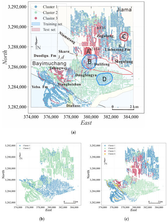
To obtain reliable supervised samples, we first applied SOM–K-means clustering to the log-transformed 39-element concentrations from the entire district. To determine the optimal number of clusters, we evaluated $K=2$, $K=3$, and $K=4$ configurations, with the corresponding spatial distributions shown in Figure 5a–c. When $K=2$, the clustering does not distinguish the principal mineralized segment from the background population, merging geochemically distinct mineralized and non-mineralized samples into a single cluster and resulting in a loss of the discriminative structure essential for subsequent supervised learning. When $K=4$, a fourth cluster emerges but accounts for only a small fraction of samples and exhibits no coherent spatial pattern or meaningful geochemical signature, indicating a geologically insignificant subdivision. In contrast, $K=3$ yields a geologically coherent and statistically supported partition. We therefore adopted $K=3$ as the final configuration, as shown in Figure 5a.

Figure 5. Spatial clustering of multi-element geochemical samples using the SOM–K-means method: (a) three clusters ($K=3$, adopted), (b) two clusters ($K=2$), and (c) four clusters ($K=4$).

We then delineated mineralized and non-mineralized zones based on the validated exploration results and fundamental metallogenic conditions, integrating SOM–K-means clustering results. Zones A and B correspond to mineralized domains with elevated ore-forming element concentrations, while Zones C and D represent distinct non-mineralized backgrounds differentiated by their host-rock geochemistry. Specifically, the mineralized zone (A and B) was delimited by areas with confirmed mineralization from drilling, whereas the non-mineralized zone (C and D) was defined based on geological assessments of metallogenic conditions and SOM–K-means clustering results. Samples within mineralized zones were treated as positive samples, and those within non-mineralized zones as negative samples [48]. Only samples with unambiguous metallogenic labels were used for supervised learning, helping to ensure the quality of the training labels.

To systematically evaluate spatial generalization, we constructed training and test sets using a spatial partition strategy. As indicated by the blue and red polygons in Figure 5, the training set comprised 150 positive and 150 negative samples from mineralized and non-mineralized zones, respectively, in the southern part of the study area, while the test set consisted of 79 positive and 79 negative samples from the spatially independent northern part. This south-for-training, north-for-test design enables an effective assessment of the model’s generalization across distinct spatial domains. All classification metrics reported in the south–north hold-out validation and ablation experiments were computed on this held-out northern test set.

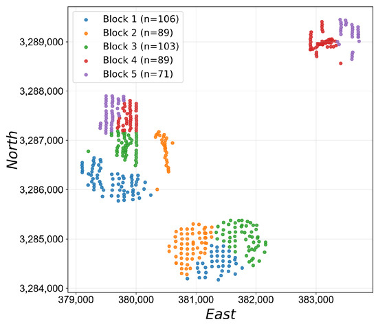
Additionally, to account for the spatial heterogeneity of MPM, we conducted five-fold stratified spatial block cross-validation on the unified supervised dataset, comprising 229 positive and 229 negative samples after merging the southern training and northern test sets. Conventional random K-fold cross-validation may place spatially adjacent and strongly autocorrelated samples in both the training and test sets, resulting in overly optimistic performance estimates. Because the positive and negative samples are largely separated in space, directly partitioning all samples into spatial clusters would produce several single-class test folds. Therefore, the two classes were separately partitioned into five geographically compact sub-blocks using K-means clustering on their coordinates, after which positive and negative sub-blocks were paired along the principal spatial axis to form five evaluation folds. As illustrated in Figure 6, each fold contains both classes while preserving spatial compactness within each class-specific sub-block. In each iteration, one paired fold was held out as the unseen test set and the remaining four folds were used for model development. The fold assignments were fixed across models, and each fold was evaluated using five random seeds, resulting in 25 model runs per model and feature subspace; the mean performance over these runs was reported.

Figure 6. Five spatial folds used for stratified spatial block cross-validation. Positive and negative samples were clustered separately by geographic coordinates and paired to ensure that every held-out fold contained both classes. Sample counts are reported in the legend.

After all independent evaluations were completed, each model was retrained on the unified supervised dataset and applied to all sampling locations to generate the final district-wide MPMs and compute the Binary Confidence (BC) metric (Section 4.4).

4.2. Definition of Metallogenic Feature Subspaces and SHAP-Based Element-Importance Quantification

According to the established metallogenic model of the Jiama district and the geochemical characteristics of the principal ore-related and pathfinder elements [48,53,54], two metallogenic feature subspaces were defined a priori on the basis of geological knowledge: the Mo–W–Sn–Bi–Se–Te assemblage (Mo-type subspace), representing an intrusion-related Mo-enriched magmatic–hydrothermal signature, and the Cu–Zn–Pb–As–Sb assemblage (Cu-type subspace), representing a Cu-polymetallic hydrothermal signature within the Jiama porphyry–skarn system.

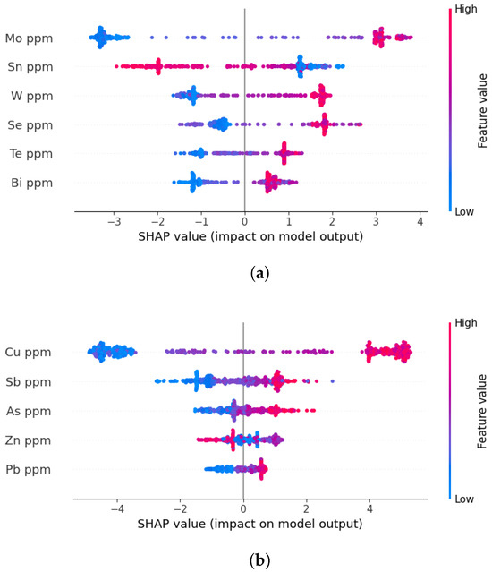
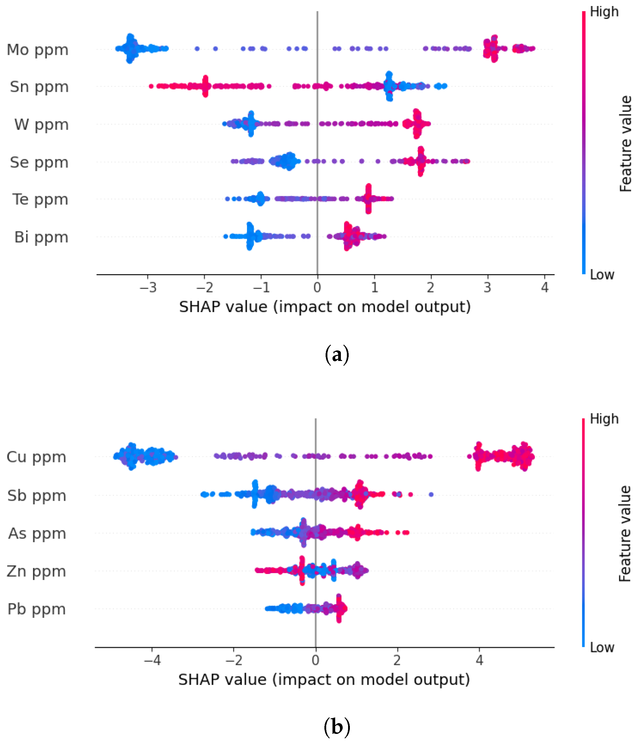
After the two metallogenic feature subspaces had been defined, separate XGBoost classifiers were trained using the elemental variables within each subspace. XGBoost is a gradient-boosted decision-tree framework capable of modeling nonlinear relationships through additive ensembles of regression trees and is relatively insensitive to feature scaling [55]. SHAP was subsequently employed to quantify the marginal contribution of each element to the predictions of the corresponding XGBoost model [56,57]. Mean absolute SHAP values were used to characterize the relative importance of the elements within each predefined metallogenic feature subspace. These values were then converted into SHAP-derived element weights and incorporated into the element-importance attention bias of SETransformer. To avoid information leakage, the SHAP values serving different roles are computed on different data partitions: (i) the SHAP-derived element weights that enter the element-importance attention bias are computed exclusively on the training data of each validation scheme—the southern training set for the south–north hold-out validation (Section 4.5.1) and the training blocks of each fold for the spatial block cross-validation (Section 4.5.2); and (ii) the SHAP analysis presented in Figure 7 is computed on the merged supervised set and is used only after the independent test-set evaluation has been completed, to support the final district-wide MPM generation; it does not enter model training or the reported test-set metrics.

Figure 7. Mean absolute SHAP values quantifying element importance within each predefined subspace, computed on the merged supervised set: (a) Mo-type subspace (Mo, W, Sn, Bi, Se, Te); (b) Cu-type subspace (Cu, Zn, Pb, As, Sb).

Within the predefined Mo-type subspace, the SHAP values quantify the relative contributions of Mo, W, Sn, Bi, Se, and Te, whereas the Cu-type analysis evaluates the contributions of Cu, Zn, Pb, As, and Sb, as shown in Figure 7a,b. The resulting importance distributions provide a data-driven characterization of element heterogeneity within each geologically defined subspace and form the basis of the SHAP-derived element weights used in SETransformer.

4.3. Experimental Settings

To ensure a fair comparison, all models were tuned under a common protocol that strictly separates hyperparameter selection from performance evaluation. For the south–north hold-out validation, hyperparameters were selected via 5-fold cross-validation on the southern training set using grid search. For spatial block cross-validation, a nested cross-validation scheme was adopted: in each outer fold, hyperparameters were selected via inner 3-fold cross-validation on the four outer-training blocks, and the optimal configuration was then used to train on all four blocks and evaluate on the held-out block. Each fold was evaluated using five random seeds, with the held-out block used only for final evaluation and excluded from all tuning steps. The fold assignments, inner-validation splits, and random seeds were identical across all compared models. The selected hyperparameter configurations obtained from the south–north hold-out training procedure are summarized in Table 1 and Appendix A for SETransformer and the baseline models, respectively. For the element-importance attention bias, SHAP-derived element weights were introduced to modulate the relative contribution of different elements during attention computation. Specifically, for the south–north hold-out validation, SHAP values were computed exclusively on the southern training set and then fixed during training and testing, and for the spatial block cross-validation, the SHAP-derived element weights were recomputed from the training blocks of each fold so that no held-out information entered the feature-weighting step.

Table 1. Hyperparameter settings of SETransformer under south–north hold-out validation.

Category	Parameter	Value
Model Hyperparameters	Embedding dimension	32
	Number of attention heads	8
	Number of element-encoder blocks	5
	Number of spatial-encoder blocks	5
	Number of Fourier bands	8
	Number of nearest neighbors	20
	Prior bias coeff. $\lambda$ (Mo-type)	5
	Prior bias coeff. $\lambda$ (Cu-type)	3
Training Hyperparameters	Epochs (Mo-type subspace)	60
	Epochs (Cu-type subspace)	80
	Learning rate (Mo-type)	$8\times {10}^{-4}$
	Learning rate (Cu-type)	$1\times {10}^{-3}$
	Weight decay (Mo-type)	$3\times {10}^{-3}$
	Weight decay (Cu-type)	$2\times {10}^{-3}$
	Batch size	256

4.4. Evaluation Metrics

Partially following the evaluation protocol of [47], we report five standard classification metrics to assess predictive performance: accuracy, recall, precision, F1 score, and Cohen’s kappa. In addition, the area under the precision–recall curve (PR-AUC) is used to evaluate ranking performance, while the Brier score is introduced to assess the quality of the predicted probabilities. Accuracy measures the overall proportion of correctly classified samples. Recall quantifies the proportion of true positives correctly identified by the model, whereas precision measures the proportion of predicted positives that are true positives. The F1 score, defined as the harmonic mean of precision and recall, provides a balanced summary of classification performance. Kappa assesses agreement between predictions and ground-truth labels beyond chance.

Let $TP$, $TN$, $FP$, and $FN$ denote the numbers of true positives, true negatives, false positives, and false negatives, respectively, and let N denote the total number of samples. The mathematical definitions of these metrics are as follows:

$$\mathrm{Accuracy}={\displaystyle \frac{TP+TN}{TP+TN+FP+FN}}$$

(22)

$$\mathrm{Recall}={\displaystyle \frac{TP}{TP+FN}}$$

(23)

$$\mathrm{Precision}={\displaystyle \frac{TP}{TP+FP}}$$

(24)

$$\mathrm{F}1\mathrm{score}=2\times {\displaystyle \frac{\mathrm{Precision}\times \mathrm{Recall}}{\mathrm{Precision}+\mathrm{Recall}}}$$

(25)

$$\mathrm{Kappa}={\displaystyle \frac{p_o-p_e}{1-p_e}}$$

(26)

where $p_o={\displaystyle \frac{TP+TN}{N}}$ is the observed agreement rate, and $p_e={\displaystyle \frac{(TP+FP)(TP+FN)+(FN+TN)(FP+TN)}{N^2}}$ is the chance agreement rate.

To evaluate probabilistic prediction quality, the Brier score is calculated as the mean squared difference between the predicted mineralization probability and the corresponding binary ground-truth label:

$$\mathrm{Brier}\mathrm{Score}={\displaystyle \frac{1}{N}}{\displaystyle \sum _{i=1}^N}{\left(p_i-y_i\right)}^2$$

(27)

where $p_i\in [0,1]$ denotes the predicted mineralization probability for the i-th sample, $y_i\in \{0,1\}$ is its ground-truth label, and N is the total number of evaluated samples. The Brier score ranges from 0 to 1, with lower values indicating that the predicted probabilities are closer to the observed outcomes. It evaluates overall probabilistic accuracy and penalizes confident but incorrect predictions more strongly than uncertain predictions. Therefore, it complements classification metrics and provides a probability-sensitive assessment of model performance.

In addition to the above classification metrics, we define an auxiliary BC index to quantify the determinacy, or sharpness, of the predicted MPMs. In binary mineral prospectivity prediction, probabilities near 0.5 correspond to ambiguous predictions near the decision boundary, whereas probabilities approaching 0 or 1 indicate a stronger assignment to non-mineralized or mineralized classes. Therefore, BC is designed to measure the average deviation of predicted probabilities from the maximally ambiguous value of 0.5:

$$\mathrm{BC}=2\times \mathbb{E}\left(\right|p-0.5\left|\right)$$

(28)

where p denotes the predicted mineralization probability for each sample, and $\mathbb{E}(·)$ denotes the mean over all samples in the study area. The factor of 2 normalizes BC to the interval $[0,1]$, where 0 indicates that all predictions are maximally ambiguous around 0.5, and 1 indicates that all predictions are fully polarized toward 0 or 1. BC does not directly measure classification correctness or probability calibration; rather, it provides a complementary description of probability-map sharpness and boundary determinacy. Therefore, BC is interpreted jointly with the classification metrics and the Brier score, with the latter used to assess whether sharper predictions are accompanied by lower probability errors.

4.5. Comparative Experiments

To comprehensively and robustly evaluate the predictive performance of the proposed model, SETransformer was compared with three conventional machine learning methods (RF, XGBoost, SVM) and two deep learning baselines (GCN [58,59] and TabNet [60]).

4.5.1. South–North Hold-Out Validation

We first evaluate all models under a south–north hold-out validation, where models are trained on the southern samples and tested on the spatially disjointed northern samples. This scheme provides a controlled first assessment of spatial transferability. All stochastic training procedures were repeated using five different random seeds. The mean performance over the five runs is reported in Table 2.

Table 2. Comparative performance of different models under the south–north hold-out validation.

Model	Accuracy (%)	Recall (%)	Precision (%)	F1 Score	Kappa
Mo-type subspace
RF	62.66	100.00	57.25	0.728	0.253
XGBoost	65.19	100.00	58.96	0.742	0.304
SVM	81.65	100.00	73.15	0.845	0.633
GCN	87.34	100.00	79.80	0.888	0.747
TabNet	85.44	100.00	78.00	0.872	0.709
SETransformer	99.37	100.00	98.75	0.994	0.987
Cu-type subspace
RF	57.59	96.20	54.29	0.694	0.152
XGBoost	73.42	100.00	65.29	0.790	0.468
SVM	79.75	100.00	71.96	0.828	0.595
GCN	87.97	100.00	80.61	0.893	0.760
TabNet	81.01	97.47	73.33	0.837	0.620
SETransformer	91.14	100.00	84.95	0.919	0.823

Note: Bold values indicate the best performance within each subspace; gray shading highlights the SETransformer model.

SETransformer achieved the best overall performance in both the Mo-type and Cu-type subspaces. In the Mo-type subspace, it attained an accuracy of 99.37%, a precision of 98.75%, an F1 score of 0.994, and a kappa value of 0.987. In the Cu-type subspace, SETransformer achieved an accuracy of 91.14%, a precision of 84.95%, an F1 score of 0.919, and a kappa value of 0.823. These results demonstrate that SETransformer provides the most accurate and balanced classification performance under the south–north hold-out validation. In comparison, RF and XGBoost maintained high recall values of 96.20%–100.00% but achieved substantially lower precision, ranging from 54.29% to 65.29%, indicating considerable overprediction of mineralized areas. SVM improved the balance between recall and precision, achieving accuracies of 81.65% and 79.75% in the Mo-type and Cu-type subspaces, respectively, but remained inferior to the deep-learning baselines. Among the baseline models, GCN exhibited the strongest overall performance, with an accuracy of 87.34% and a kappa value of 0.747 in the Mo-type subspace, and 87.97% and 0.760 in the Cu-type subspace, whereas TabNet achieved accuracies of 85.44% and 81.01%.

4.5.2. Spatial Block Cross-Validation

To further assess model robustness under spatial heterogeneity and reduce the optimistic bias potentially caused by spatial autocorrelation, all models were evaluated using five-fold spatial block cross-validation. Each spatial fold was repeated using five random seeds, resulting in 25 runs for each model and metallogenic feature subspace. The averaged results are summarized in Table 3.

Table 3. Comparative performance of different models under five-fold spatial block cross-validation.

Model	PR-AUC	Accuracy (%)	Precision (%)	Recall (%)	F1 Score	Kappa	Brier Score
Mo-type subspace
RF	0.989	85.28	85.63	90.25	0.861	0.694	0.094
XGBoost	0.985	83.67	83.92	91.30	0.855	0.663	0.116
SVM	0.937	83.11	84.47	88.07	0.840	0.653	0.134
TabNet	0.974	85.85	82.96	94.33	0.873	0.712	0.120
GCN	1.000	90.34	87.91	100.00	0.925	0.805	0.155
SETransformer	1.000	98.53	98.26	100.00	0.990	0.963	0.014
Cu-type subspace
RF	0.878	79.12	79.97	89.98	0.829	0.570	0.145
XGBoost	0.888	82.68	83.69	89.31	0.848	0.645	0.135
SVM	0.914	79.94	81.42	87.85	0.828	0.590	0.153
TabNet	0.876	80.37	77.91	91.29	0.834	0.590	0.178
GCN	0.978	89.70	90.15	93.59	0.903	0.785	0.164
SETransformer	1.000	90.61	88.80	100.00	0.931	0.801	0.065

Note: Bold values indicate the best performance within each subspace; gray shading highlights the SETransformer model.

In the Mo-type subspace, SETransformer achieved the best overall performance, with a PR-AUC of 1.000, an accuracy of 98.53%, a precision of 98.26%, a recall of 100.00%, an F1 score of 0.990, and a kappa value of 0.963. Although GCN also obtained a PR-AUC of 1.000 and a recall of 100.00%, its accuracy, precision, F1 score, and kappa were only 90.34%, 87.91%, 0.925, and 0.805, respectively. Compared with GCN, SETransformer improved accuracy by 8.19 percentage points, precision by 10.35 percentage points, and kappa by 0.158. This indicates that, although both models can rank positive samples effectively, SETransformer converts this ranking ability into substantially more accurate class assignments and fewer false-positive predictions.

SETransformer also achieved the lowest Brier score in the Mo-type subspace, decreasing from 0.094 for the best-performing baseline in terms of Brier score to 0.014. The combination of a high PR-AUC and a low Brier score indicates that the model not only discriminates mineralized from non-mineralized samples effectively but also produces probability estimates that are more consistent with the observed labels. In contrast, the relatively high Brier score of GCN, despite its PR-AUC of 1.000, suggests that strong ranking performance does not necessarily correspond to accurate probability estimates.

In the Cu-type subspace, SETransformer again exhibited the strongest overall performance, achieving a PR-AUC of 1.000, an accuracy of 90.61%, a recall of 100.00%, an F1 score of 0.931, a kappa value of 0.801, and a Brier score of 0.065. GCN was the closest competing model, with a PR-AUC of 0.978, an accuracy of 89.70%, a recall of 93.59%, an F1 score of 0.903, and a kappa value of 0.785. Although GCN obtained a slightly higher precision than SETransformer (90.15% versus 88.80%), this improvement was accompanied by a lower recall. SETransformer therefore achieved a better balance between recovering mineralized samples and controlling false-positive predictions, as reflected by its higher F1 score and kappa value.

The advantage of SETransformer in the Cu-type subspace is particularly evident in probability estimation. Its Brier score of 0.065 was substantially lower than those of the baseline models, which ranged from 0.135 to 0.178. This result indicates that the high-confidence predictions produced by SETransformer are not attributable solely to greater probability sharpness, but are accompanied by smaller probability errors on the held-out spatial blocks.

The spatial block cross-validation results are also consistent with those obtained from the independent south–north hold-out validation. For SETransformer, accuracy decreased only slightly from 99.37% to 98.53% in the Mo-type subspace and from 91.14% to 90.61% in the Cu-type subspace. Similarly, kappa decreased from 0.987 to 0.963 for the Mo-type subspace and from 0.823 to 0.801 for the Cu-type subspace. The limited performance variation between the two spatial validation schemes indicates that the superior performance of SETransformer is not restricted to a single favorable south-north partition.

4.5.3. District-Wide MPM Generation and Probability-Map Sharpness

After completion of the independent south–north hold-out and spatial block cross-validation experiments, each model was retrained on the unified supervised dataset and applied to all district-wide sampling locations to generate the final mineral prospectivity maps. The BC values of the resulting district-wide MPMs are reported in Table 4. SETransformer obtained BC values of 0.936 and 0.968 for the Mo-type and Cu-type subspaces, respectively, exceeding the corresponding values of the baseline models. These values indicate stronger probability polarization and sharper contrasts between high- and low-probability areas. However, BC is interpreted only as a descriptive measure of map sharpness and does not independently establish classification correctness, probability calibration, or model reliability.

Table 4. Binary Confidence of the final district-wide MPMs generated after retraining on the unified supervised dataset.

Model	Mo-Type Subspace	Cu-Type Subspace
RF	0.805	0.700
XGBoost	0.911	0.706
SVM	0.864	0.774
GCN	0.895	0.836
TabNet	0.901	0.848
SETransformer	0.936	0.968

Note: Bold values indicate the highest BC values; gray shading highlights the SETransformer model.

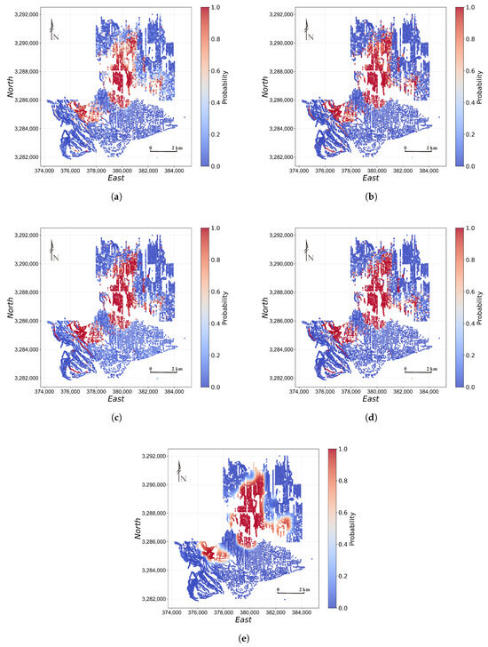
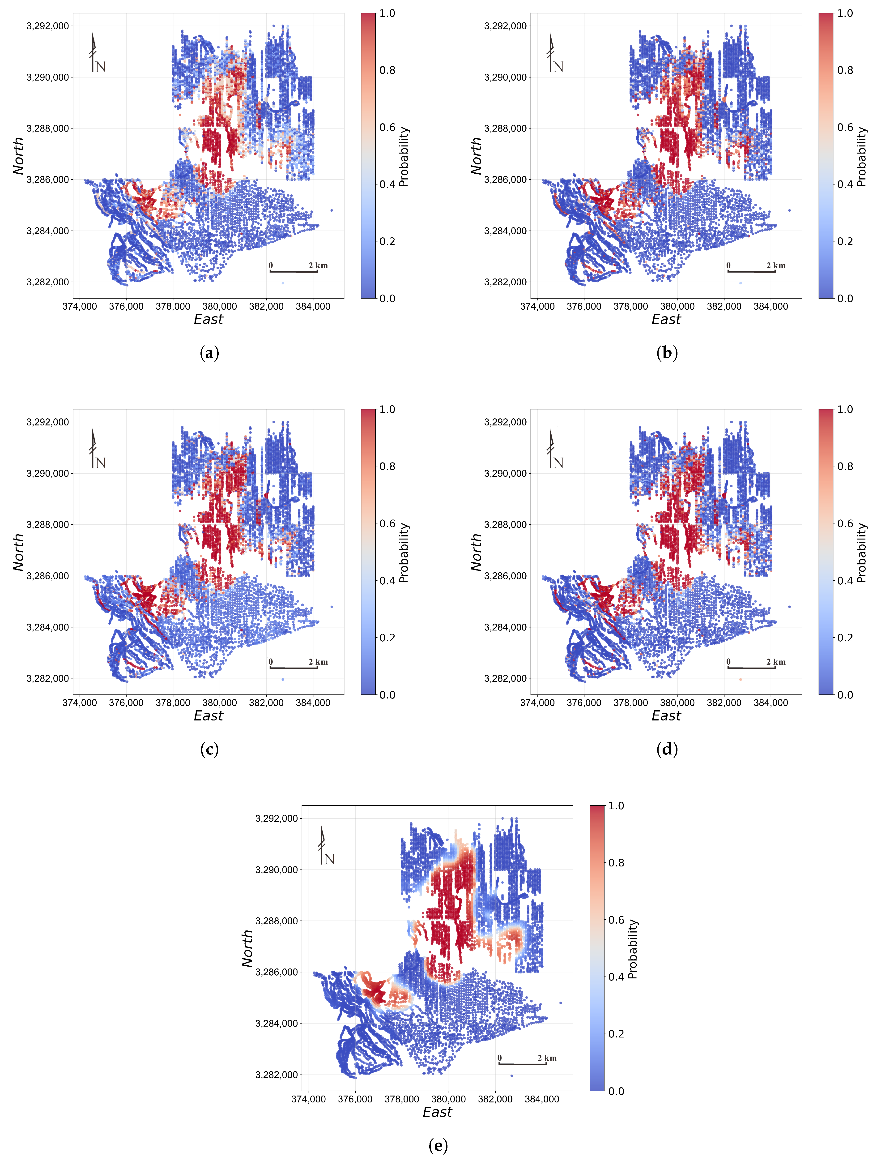
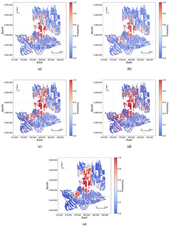
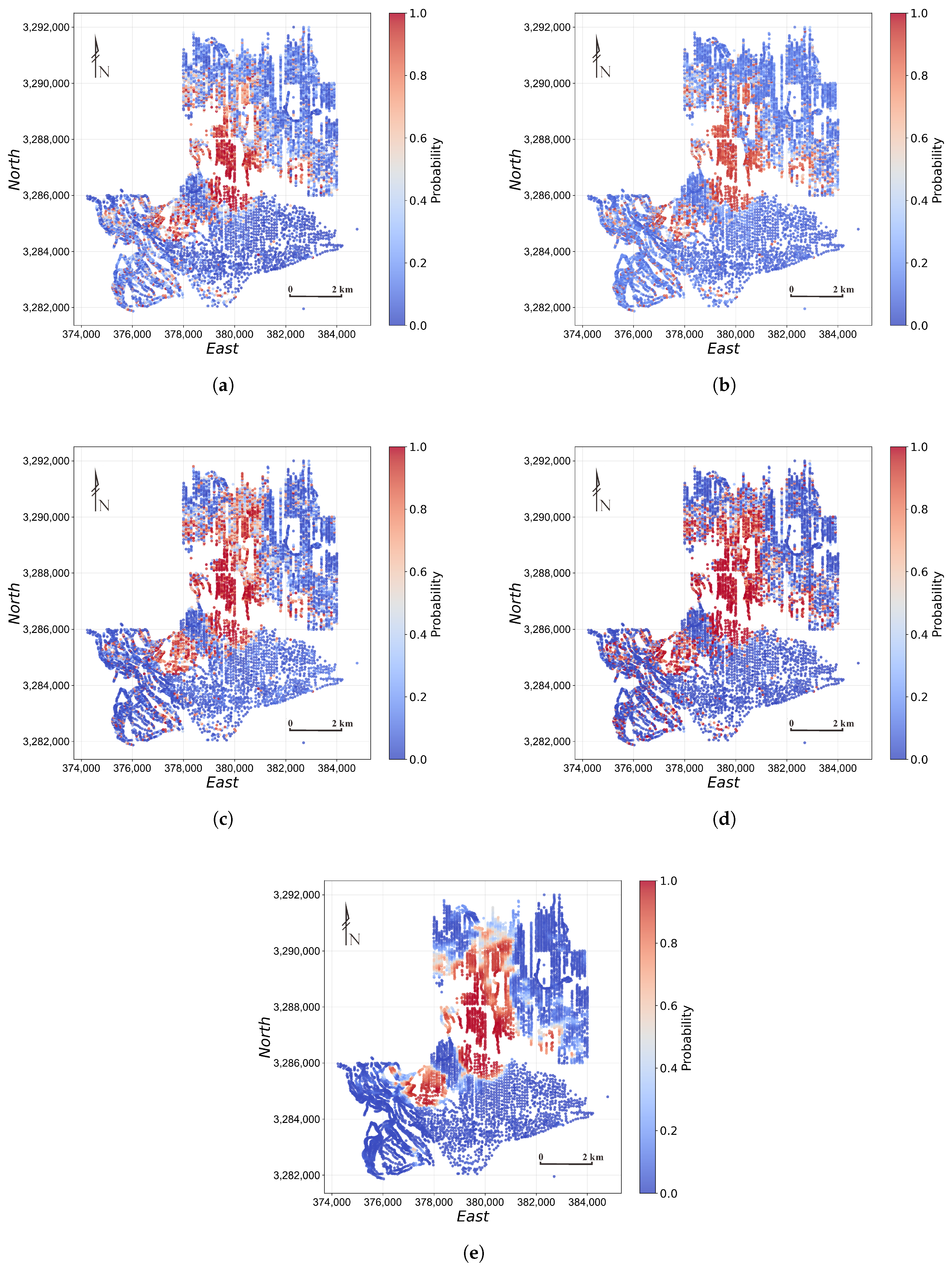
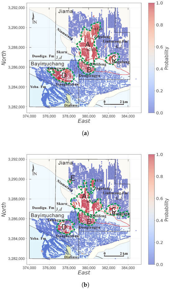
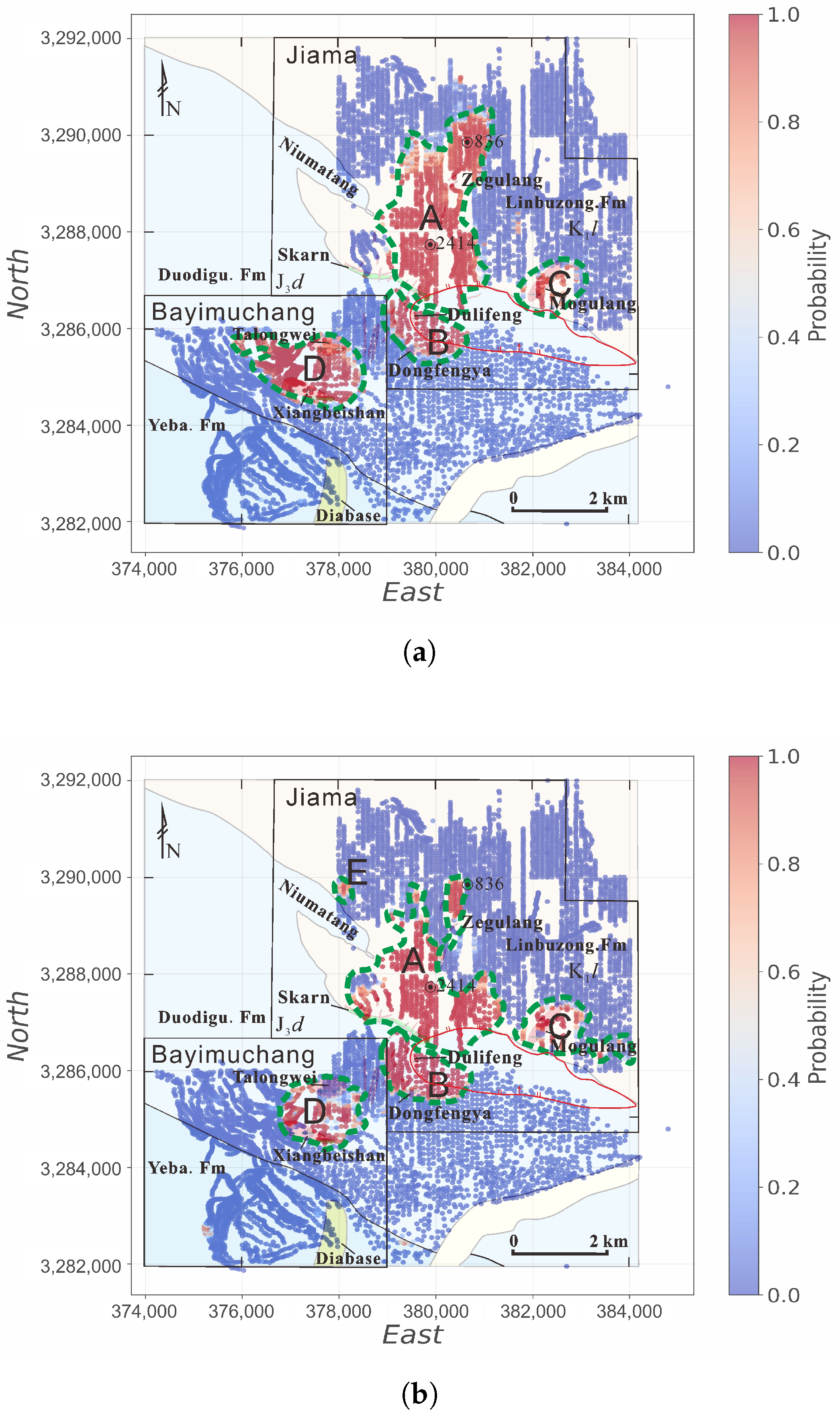
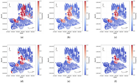
The final MPMs reveal distinct spatial patterns among the models (Figure 8, Figure 9 and Figure 10). RF, XGBoost, and SVM identify the principal anomalous zones but also produce dispersed high-probability responses in surrounding background areas. TabNet generates relatively fragmented prediction patterns, whereas GCN produces spatially continuous zones with comparatively broad probability transitions. SETransformer concentrates high-probability responses within the known mineralized belts and adjacent geologically favorable areas, producing more compact and continuous prospective zones with sharper boundaries. The geological consistency of these maps is assessed from their spatial relationship with known mineralization and favorable geological features, rather than from BC alone.

Figure 8. Comparison of district-wide MPMs generated by the baseline models using the Mo-type subspace: (a) RF, (b) XGBoost, (c) SVM, (d) TabNet, and (e) GCN.

Figure 9. Comparison of district-wide MPMs generated by the baseline models using the Cu-type subspace: (a) RF, (b) XGBoost, (c) SVM, (d) TabNet, and (e) GCN.

Figure 10. District-wide MPMs generated by SETransformer after retraining on the unified supervised dataset: (a) Mo-type subspace and (b) Cu-type subspace. The five labeled high-prospectivity regions in panel (b) are A, Jiama–Zegulang; B, Dongfengya–Dulifeng; C, Mogulang; D, Talongwei–Xiangbeishan; and E, Niumatang. These prospective regions are discussed in Section 5.

4.6. Ablation

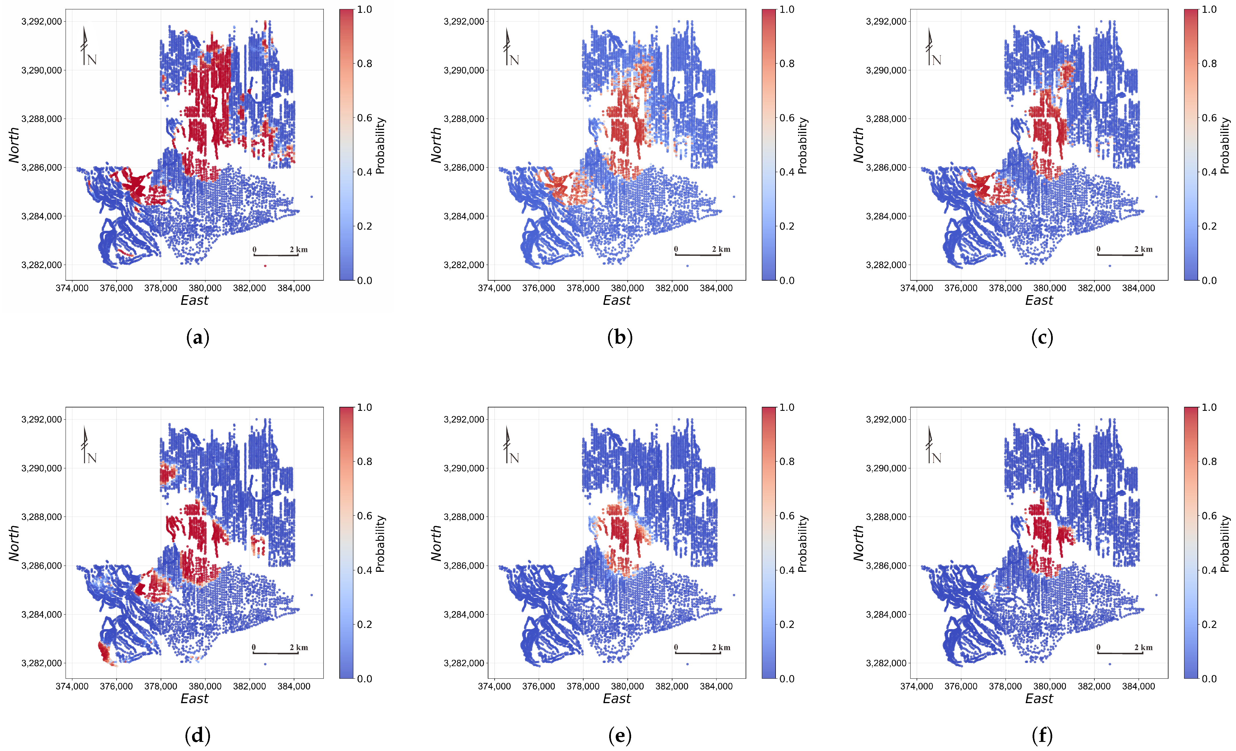
To isolate the contributions of the proposed components, we conducted component-level ablation experiments in both the Mo-type and Cu-type subspaces while keeping the encoder architecture and trainable capacity unchanged. Three variants were evaluated: (1)w/ uniform element weights, in which the SHAP-derived element weights were replaced by uniform values; (2) w/o KNN mask, in which the neighborhood constraint was removed while retaining distance-decay factor; and (3) w/o distance-decay factor, in which all KNN neighbors were assigned equal decay factors. The results are presented in Table 5 and Figure 11.

Table 5. Ablation study results under south–north hold-out validation and Binary Confidence of the final district-wide MPMs.

Model	Accuracy (%)	Recall (%)	Precision (%)	F1 Score	Kappa	BC
Mo-type subspace
Ours w/ uniform element weights	72.15	100.00	64.23	0.782	0.443	0.888
Ours w/o KNN mask	95.57	100.00	91.86	0.958	0.911	0.825
Ours w/o distance-decay factor	93.04	100.00	87.78	0.935	0.861	0.917
Ours	99.37	100.00	98.75	0.994	0.987	0.936
Cu-type subspace
Ours w/ uniform element weights	70.89	96.20	63.87	0.768	0.418	0.953
Ours w/o KNN mask	51.27	100.00	50.64	0.672	0.025	0.942
Ours w/o distance-decay factor	75.95	100.00	67.52	0.806	0.519	0.978
Ours	91.14	100.00	84.95	0.919	0.823	0.968

Note: Bold values indicate the best performance within each subspace; gray shading highlights the complete SETransformer model.

Figure 11. Component-level ablation MPMs for the Mo-type subspace: (a) uniform element weights, (b) without the KNN mask, and (c) without the distance-decay factor. Panels (d–f) show the corresponding results for the Cu-type subspace.

In the Mo-type subspace, replacing the SHAP-derived element weights with uniform element weights produces the largest degradation. Accuracy decreases from 99.37% to 72.15%, precision from 98.75% to 64.23%, F1 Score from 0.994 to 0.782, and kappa from 0.987 to 0.443. This result demonstrates that explicitly incorporating element-importance heterogeneity is critical for distinguishing the Mo–W–Sn–Bi–Se–Te mineralization signature from the geochemical background. Removing the KNN mask or the distance-decay term causes smaller but still consistent decreases. Without the KNN mask, accuracy and kappa decline to 95.57% and 0.911, respectively; without distance-decay factor, they decrease to 93.04% and 0.861. Thus, both local-neighborhood restriction and distance-sensitive weighting contribute to Mo-type prediction, with the decay term providing additional discrimination among samples within the selected neighborhood.

The Cu-type subspace shows a different sensitivity pattern. Removing the KNN mask causes the most severe deterioration: accuracy drops from 91.14% to 51.27%, precision from 84.95% to 50.64%, F1 score from 0.919 to 0.672, and kappa from 0.823 to 0.025. The near-zero kappa indicates that unconstrained all-to-all spatial interaction introduces substantial background interference and largely eliminates agreement beyond chance. Removing the SHAP-derived element weights also causes a marked reduction, with accuracy, precision, F1 score, and kappa decreasing to 70.89%, 63.87%, 0.768, and 0.418, respectively. When only the distance-decay term is removed, the corresponding values decrease to 75.95%, 67.52%, 0.806, and 0.519. These results indicate that the Cu–Zn–Pb–As–Sb assemblage requires both element-level importance guidance and strongly localized spatial aggregation, and that the KNN mask is particularly important for suppressing spatially distant and weakly related geochemical signals.

From the perspective of the resulting MPMs (Figure 11), replacing the SHAP-derived element weights with uniform element weights produces broader and more fragmented high-probability zones, indicating weaker localization of the dominant metallogenic signatures. Removing the KNN mask reduces the spatial extent of the predicted favorable areas and leads to less coherent local probability transitions and less distinct prospectivity boundaries, suggesting that unconstrained spatial interactions weaken the representation of local anomaly structure. Removing the distance-decay factor also contracts the predicted favorable areas, but the principal high-probability cores and their boundaries remain relatively clear, indicating that distance-dependent weighting mainly helps preserve peripheral and secondary prospective anomalies.

5. Discussion

The central finding of this study is that, for irregularly sampled geochemical data, jointly modeling element-contribution heterogeneity and spatial dependence produces more accurate and spatially coherent MPMs. In both the Mo-type and Cu-type subspaces, SETransformer consistently outperforms conventional machine learning and deep learning baselines, achieving higher classification performance and generating MPMs with sharper boundaries and greater contrast between prospective and background zones.

This advantage arises from the complementarity between element-wise attention and spatial attention, as demonstrated quantitatively by ablation experiments. Ablation results show that disabling any individual component—the SHAP-derived element weights, the KNN mask, or the distance-decay factor—causes a consistent performance decline, though the dominant component differs between the two subspaces: replacing the SHAP-derived element weights with uniform weights causes the largest degradation in the Mo-type subspace, whereas removing the KNN mask is the most detrimental in the Cu-type subspace. Because all ablation variants retain the same architecture and trainable capacity, these results indicate that SETransformer’s performance gain stems from jointly modeling element-contribution heterogeneity and neighborhood-scale spatial dependence, rather than merely from increased model capacity. By comparison, baseline models capture only part of this joint information. RF and XGBoost treat elements independently and lack spatial modeling, yielding high recall but low precision due to over-prediction in weakly anomalous background areas. SVM improves decision-boundary flexibility through its nonlinear kernel but still lacks mechanisms for jointly modeling element and spatial dependencies. GCN and TabNet emphasize graph-based neighborhood aggregation and sequential feature selection, respectively, which limits their ability to capture both dependencies simultaneously; accordingly, their precision and kappa remain lower than those of SETransformer.

Under the south–north hold-out validation, recall is generally high across both subspaces, ranging from 96% to 100% for the evaluated models. The labeled positive samples were delineated by interpreting SOM–K-means patterns jointly with drill-confirmed mineralization and geological constraints. They therefore largely represent pronounced geochemical anomalies characterized by enrichment in ore-related elements and strong contrast relative to the background, making them comparatively easy for the models to detect and resulting in few false-negative predictions. Despite this high recall, RF, XGBoost, and SVM achieve only approximately 54%–73% precision, indicating that many background samples are incorrectly classified as mineralized. This likely occurs because some background samples contain weak or locally elevated geochemical signals that resemble the positive class, whereas these models cannot simultaneously account for element-contribution heterogeneity and local spatial context. Recall alone therefore provides limited discrimination among the models. Predictive performance is interpreted primarily using precision, F1 score, kappa, PR-AUC, and the Brier score.

Under the spatial block cross-validation setting, the models exhibit a clear three-tier separation (Table 3). Because PR-AUC is a threshold-independent ranking metric that is nearly saturated in this task, the differences among models are reflected primarily in the decision-level metrics (accuracy, precision, kappa) and in probability quality (Brier score). The conventional machine learning models (RF, XGBoost, SVM) and TabNet form the lowest tier, with broadly comparable performance (kappa ∼0.65–0.71 in the Mo-type and ∼0.57–0.65 in the Cu-type subspace), because none of them explicitly represents spatial dependence among sampling locations—RF, XGBoost, and SVM treat each sample independently, and although TabNet applies sequential attention over features, it likewise operates on individual samples without a spatial neighborhood—so that under spatially blocked partitions they cannot exploit spatial continuity and converge to a similar, moderate level. GCN occupies the intermediate tier (kappa 0.805 and 0.785) by aggregating information over spatial neighborhoods and thus partially capturing spatial autocorrelation, yet it does not jointly model element-contribution heterogeneity and remains poorly calibrated (Brier score 0.155 and 0.164) despite its strong ranking ability. SETransformer achieves the highest tier, surpassing GCN in almost all metrics and attaining substantially lower Brier scores (0.014 and 0.065), because it jointly models element-contribution heterogeneity and neighborhood-scale spatial dependence; The combination of strong discrimination and low probability error indicates that SETransformer’s decisive predictions are accompanied by smaller probabilistic errors, reducing the concern of overconfident incorrect predictions.

It is also worth noting that the conventional baselines, particularly RF and XGBoost, achieve markedly higher overall metrics under the spatial block cross-validation than under the south–north hold-out validation (e.g., the kappa of RF in the Mo-type subspace increases from 0.253 to 0.694). This does not imply that spatial block cross-validation is a less demanding test; rather, it reflects the different nature of the two spatial settings. The south–north hold-out validation is an extreme one-directional extrapolation, in which the entire test region lies outside the spatial extent of the training data and may exhibit a systematic shift in geochemical background. Models without spatial modeling, such as RF and XGBoost, fit the training distribution directly and therefore degrade substantially under this distribution shift. In contrast, the spatially blocked folds are distributed across the whole district, so each held-out block is surrounded by training blocks and shares a more similar geochemical background, alleviating the distribution shift and allowing these distribution-sensitive models to recover. Notably, SETransformer exhibits only a marginal change between the two schemes (e.g., Mo-type kappa 0.987 vs. 0.963), whereas the conventional baselines fluctuate strongly; this contrast further indicates that the performance of SETransformer is stable across fundamentally different spatial partitions, rather than tuned to a single favorable split.

In terms of target delineation, the proposed workflow identifies multiple high-prospectivity zones in and around the Jiama district. In the Mo-type subspace, four high-prospectivity regions (A–D) are identified (Figure 10a): Jiama–Zegulang, Dongfengya–Dulifeng, Mogulang, and Talongwei–Xiangbeishan. These zones are spatially concentrated and show good agreement with existing geological evidence [48,54]. Among them, the Jiama–Zegulang target is consistent with existing exploration results and corresponds to the main exploration and evaluation area of the Jiama deposit, where the spatial distribution of orebodies has been confirmed [48]. The Talongwei–Xiangbeishan target is also characterized by intermediate-to-felsic intrusions [61], and surface mapping and partial drilling have verified favorable porphyry–skarn Cu-polymetallic mineralization potential in this area [48]. In addition, previous geological surveys indicate that the Dongfengya–Dulifeng and Mogulang targets also contain intermediate-to-felsic intrusions and exhibit evident sericitization alteration [61], suggesting that they may represent important exploration targets.

In the Cu-type subspace, five high-prospectivity regions (A–E) are identified (Figure 10b): Jiama–Zegulang, Dongfengya–Dulifeng, Mogulang, Talongwei–Xiangbeishan, and Niumatang [48]. The first four targets are broadly consistent with those identified in the Mo-type subspace, although the morphology of the predicted high-prospectivity zones differs slightly. This difference may be related to the geochemical characteristics of the selected element assemblages. Mo-related assemblages are more representative of intermediate- to high-temperature geochemical associations and therefore tend to highlight the magmatic–hydrothermal center more clearly [62,63,64,65]. In contrast, Cu-related assemblages are relatively more characteristic of intermediate- to low-temperature associations and may therefore show a more spatially dispersed distribution pattern [64]. Notably, the Cu-type subspace additionally delineates the Niumatang target, which may be associated with limited skarn alteration outcrops in this area [64]. This target warrants further geological verification, especially because an independent high-grade gold orebody has also been reported nearby in previous studies [66].

From the perspective of exploration practice, BC characterizes the overall sharpness of the final MPMs and the probability contrast between predicted high- and low-prospectivity areas. Because BC does not measure prediction correctness or probability calibration, it is interpreted separately from the held-out probabilistic evaluation. Under spatial block cross-validation, SETransformer achieved the lowest Brier score among all compared models, indicating smaller overall probability errors and reducing the concern that its decisive predictions arise solely from overconfident incorrect estimates. When integrated with metallogenic and geological analysis, the SETransformer workflow can support the delineation and prioritization of prospective targets within the Jiama district and its surrounding areas. Future work will apply this workflow to other mineralized regions to further evaluate its generalizability under different geological settings.

6. Conclusions

This study develops a geochemistry-based workflow for MPM and proposes a supervised SETransformer model. The main conclusions are as follows: (1) SOM–K-means clustering identified broad geochemical populations and provided auxiliary support for sample delineation. Positive and negative samples were selected based on drill-confirmed mineralization and geological interpretation, yielding geologically constrained class labels for supervised modeling.

(2) Two metallogenic feature subspaces, Mo-type and Cu-type, were defined a priori based on the regional metallogenic context, providing geologically interpretable representations of distinct mineralization signatures.

(3) SETransformer integrates an element encoder and a spatial encoder. The element-importance attention bias emphasizes diagnostically informative element associations, whereas adaptive-bandwidth spatial-decay attention captures local spatial continuity. Ablation results demonstrated the contributions of the SHAP-derived element weights, the KNN mask, and the distance-decay factor. SETransformer outperformed the five baseline models and generated more geologically coherent MPMs.

(4) The resulting MPMs were consistent with existing geological evidence and delineated prospective zones with clear boundaries, providing a useful basis for subsequent exploration-target prioritization.

References

- Zhai, M.; Hu, B. Thinking to state security, international competition and national strategy of mineral resources. J. Earth Sci. Environ. 2021, 43, 1–11. [Google Scholar] [CrossRef]
- Harris, J.; Grunsky, E.; Behnia, P.; Corrigan, D. Data- and knowledge-driven mineral prospectivity maps for Canada’s North. Ore Geol. Rev. 2015, 71, 788–803. [Google Scholar] [CrossRef] [Scilit]
- Yousefi, M.; Nykänen, V. Introduction to the special issue: GIS-based mineral potential targeting. J. Afr. Earth Sci. 2017, 128, 1–4. [Google Scholar] [CrossRef] [Scilit]
- Sun, T.; Chen, F.; Zhong, L.; Liu, W.; Wang, Y. GIS-based mineral prospectivity mapping using machine learning methods: A case study from Tongling ore district, eastern China. Ore Geol. Rev. 2019, 109, 26–49. [Google Scholar] [CrossRef] [Scilit]
- Yang, N.; Zhang, Z.; Yang, J.; Hong, Z.; Shi, J. A Convolutional Neural Network of GoogLeNet Applied in Mineral Prospectivity Prediction Based on Multi-source Geoinformation. Nat. Resour. Res. 2021, 30, 3905–3923. [Google Scholar] [CrossRef] [Scilit]
- Bonham-Carter, G. Geographic Information Systems for Geoscientists: Modelling with GIS; Computer Methods in the Geosciences, Elsevier Science & Technology Books; Elsevier: Amsterdam, The Netherlands, 1994. [Google Scholar]
- Zhao, P.; Cheng, Q.; Xia, Q. Quantitative Prediction for Deep Mineral Exploration. J. China Univ. Geosci. 2008, 19, 309–318. [Google Scholar] [CrossRef] [Scilit]
- Carranza, E.J.M. Geocomputation of mineral exploration targets. Comput. Geosci. 2011, 37, 1907–1916. [Google Scholar] [CrossRef] [Scilit]
- Parsa, M.; Carranza, E.J.M. Modulating the Impacts of Stochastic Uncertainties Linked to Deposit Locations in Data-Driven Predictive Mapping of Mineral Prospectivity. Nat. Resour. Res. 2021, 30, 3081–3097. [Google Scholar] [CrossRef] [Scilit]
- Wang, W.; Zhao, J.; Cheng, Q.; Carranza, E.J.M. GIS-based mineral potential modeling by advanced spatial analytical methods in the southeastern Yunnan mineral district, China. Ore Geol. Rev. 2015, 71, 735–748. [Google Scholar] [CrossRef] [Scilit]
- Feng, Y.; Wang, Y.; Wang, C.; Tian, J.; Wen, S.; Zhou, Y.; Cheng, Y. A Fuzzy Gold Mineral Prediction Model Integrating with Knowledge-Driven and Data-Driven: A Case Study of the Hatu Region in Xinjiang, China. Minerals 2024, 14, 1209. [Google Scholar] [CrossRef] [Scilit]
- Sheng, S.; Wang, Y.; Tian, J.; Chen, X.; Ning, Y.; Dong, Y.; An, Z. Knowledge–Data Collaboration-Driven Mineral Prospectivity Prediction with Graph Attention Networks. Minerals 2025, 15, 1164. [Google Scholar] [CrossRef] [Scilit]
- Zuo, R.; Yang, F.; Cheng, Q.; Kreuzer, O.P. A novel data-knowledge dual-driven model coupling artificial intelligence with a mineral systems approach for mineral prospectivity mapping. Geology 2025, 53, 284–288. [Google Scholar] [CrossRef] [Scilit]
- Wang, L.; Li, T.; Wu, S.; Yang, J.; Hu, Y.; Hu, L.; Chen, Y.; Ge, Y.; Chen, Y.; Rao, C.; et al. Geologically constrained data-driven modeling for mineral prospectivity mapping. Geology 2026, 54, 225–230. [Google Scholar] [CrossRef] [Scilit]
- Fu, Z.; Zheng, X.; Yan, Y.; Xu, X.; Zhou, F.; Li, X.; Zhou, Q.; Mai, W. The Evolution of Machine Learning in Large-Scale Mineral Prospectivity Prediction: A Decade of Innovation (2016–2025). Minerals 2025, 15, 1042. [Google Scholar] [CrossRef] [Scilit]
- Rodriguez-Galiano, V.; Sanchez-Castillo, M.; Chica-Olmo, M.; Chica-Rivas, M. Machine learning predictive models for mineral prospectivity: An evaluation of neural networks, random forest, regression trees and support vector machines. Ore Geol. Rev. 2015, 71, 804–818. [Google Scholar] [CrossRef] [Scilit]
- Carranza, E.J.M.; Laborte, A.G. Random forest predictive modeling of mineral prospectivity with small number of prospects and data with missing values in Abra (Philippines). Comput. Geosci. 2015, 74, 60–70. [Google Scholar] [CrossRef] [Scilit]
- Maepa, F.; Smith, R.S.; Tessema, A. Support vector machine and artificial neural network modelling of orogenic gold prospectivity mapping in the Swayze greenstone belt, Ontario, Canada. Ore Geol. Rev. 2021, 130, 103968. [Google Scholar] [CrossRef] [Scilit]
- Parsa, M. A data augmentation approach to XGboost-based mineral potential mapping: An example of carbonate-hosted ZnPb mineral systems of Western Iran. J. Geochem. Explor. 2021, 228, 106811. [Google Scholar] [CrossRef] [Scilit]
- Sihombing, F.M.; Palin, R.M.; Hughes, H.S.; Robb, L.J. Improved mineral prospectivity mapping using graph neural networks. Ore Geol. Rev. 2024, 172, 106215. [Google Scholar] [CrossRef] [Scilit]
- Xiong, Y.; Zuo, R. GIS-based rare events logistic regression for mineral prospectivity mapping. Comput. Geosci. 2018, 111, 18–25. [Google Scholar] [CrossRef] [Scilit]
- Zhang, D.; Ren, N.; Hou, X. An improved logistic regression model based on a spatially weighted technique (ILRBSWT v1.0) and its application to mineral prospectivity mapping. Geosci. Model Dev. 2018, 11, 2525–2539. [Google Scholar] [CrossRef] [Scilit]
- Zuo, R.; Carranza, E.J.M. Support vector machine: A tool for mapping mineral prospectivity. Comput. Geosci. 2011, 37, 1967–1975. [Google Scholar] [CrossRef] [Scilit]
- Chen, G.; Huang, N.; Wu, G.; Luo, L.; Wang, D.; Cheng, Q. Mineral prospectivity mapping based on wavelet neural network and Monte Carlo simulations in the Nanling W-Sn metallogenic province. Ore Geol. Rev. 2022, 143, 104765. [Google Scholar] [CrossRef] [Scilit]
- Seyedrahimi-Niaraq, M.; Mahdiyanfar, H.; Olyaee, M.H. Comparison of the performance of gradient boost, linear regression, decision tree, and voting algorithms to separate geochemical anomalies areas in the fractal environment. Artif. Intell. Geosci. 2025, 6, 100156. [Google Scholar] [CrossRef] [Scilit]
- Talebi, H.; Peeters, L.J.; Otto, A.; Tolosana-Delgado, R. A Truly Spatial Random Forests Algorithm for Geoscience Data Analysis and Modelling. Math. Geosci. 2022, 54, 1–22. [Google Scholar] [CrossRef] [Scilit]
- Lee, S.; Moon, I. Recent Advances and Future Perspectives of AI-Based Mineral Exploration: A Review of Machine Learning, Deep Learning, and Geologically Informed Approaches. Minerals 2026, 16, 584. [Google Scholar] [CrossRef] [Scilit]
- Sun, K.; Chen, Y.; Geng, G.; Lu, Z.; Zhang, W.; Song, Z.; Guan, J.; Zhao, Y.; Zhang, Z. A Review of Mineral Prospectivity Mapping Using Deep Learning. Minerals 2024, 14, 1021. [Google Scholar] [CrossRef] [Scilit]
- Zhang, Y.; Chen, J.; Jia, Z.; Li, S.; Liu, S.; Zhang, Z.; Zhang, Y. Construction and prediction of a prospecting model based on recurrent neural network. Geol. Bull. China 2019, 38, 2033–2042. [Google Scholar]
- Wang, Z.; Zuo, R. Mineral prospectivity mapping using a joint singularity-based weighting method and long short-term memory network. Comput. Geosci. 2022, 158, 104974. [Google Scholar] [CrossRef] [Scilit]
- Yin, B.; Zuo, R.; Xiong, Y. Mineral prospectivity mapping via gated recurrent unit model. Nat. Resour. Res. 2022, 31, 2065–2079. [Google Scholar] [CrossRef] [Scilit]
- Xiong, Y.; Zuo, R. Recognition of geochemical anomalies using a deep autoencoder network. Comput. Geosci. 2016, 86, 75–82. [Google Scholar] [CrossRef] [Scilit]
- Jordao, H.; Azevedo, L.; Sousa, A.J.; Soares, A. Generative Adversarial Network Applied to Ore Type Modeling in Complex Geological Environments. Math. Geosci. 2022, 54, 1165–1182. [Google Scholar] [CrossRef] [Scilit]
- Li, T.; Zuo, R.; Zhao, X.; Zhao, K. Mapping prospectivity for regolith-hosted REE deposits via convolutional neural network with generative adversarial network augmented data. Ore Geol. Rev. 2022, 142, 104693. [Google Scholar] [CrossRef] [Scilit]
- Guo, M.; Chen, Y. A SMOTified-GAN-augmented bagging ensemble model of extreme learning machines for detecting geochemical anomalies associated with mineralization. Geochemistry 2024, 84, 126156. [Google Scholar] [CrossRef] [Scilit]
- Liu, Y.; Zhu, L.; Zhou, Y. Application of Convolutional Neural Network in prospecting prediction of ore deposits: Taking the Zhaojikou Pb-Zn ore deposit in Anhui Province as a case. Acta Petrol. Sin. 2018, 34, 3217–3224. [Google Scholar]
- Xu, Y.; Li, Z.; Xie, Z.; Cai, H.; Niu, P.; Liu, H. Mineral prospectivity mapping by deep learning method in Yawan-Daqiao area, Gansu. Ore Geol. Rev. 2021, 138, 104316. [Google Scholar] [CrossRef] [Scilit]
- Li, S.; Chen, J.; Xiang, J. Applications of deep convolutional neural networks in prospecting prediction based on two-dimensional geological big data. Neural Comput. Appl. 2020, 32, 2037–2053. [Google Scholar] [CrossRef] [Scilit]
- Yang, N.; Zhang, Z.; Yang, J.; Hong, Z. Applications of data augmentation in mineral prospectivity prediction based on convolutional neural networks. Comput. Geosci. 2022, 161, 105075. [Google Scholar] [CrossRef] [Scilit]
- Gao, L.; Huang, Y.; Zhang, X.; Liu, Q.; Chen, Z. Prediction of Prospecting Target Based on ResNet Convolutional Neural Network. Appl. Sci. 2022, 12, 11433. [Google Scholar] [CrossRef] [Scilit]
- Liu, C.; Wang, W.; Tang, J.; Wang, Q.; Zheng, K.; Sun, Y.; Zhang, J.; Gan, F.; Cao, B. A deep-learning-based mineral prospectivity modeling framework and workflow in prediction of porphyry–epithermal mineralization in the Duolong ore District, Tibet. Ore Geol. Rev. 2023, 157, 105419. [Google Scholar] [CrossRef] [Scilit]
- Yin, B.; Zuo, R.; Sun, S. Mineral Prospectivity Mapping Using Deep Self-Attention Model. Nat. Resour. Res. 2023, 32, 37–56. [Google Scholar] [CrossRef] [Scilit]
- Li, C.; Xiao, K.; Sun, L.; Tang, R.; Dong, X.; Qiao, B.; Xu, D. CNN-Transformers for mineral prospectivity mapping in the Maodeng–Baiyinchagan area, Southern Great Xing’an Range. Ore Geol. Rev. 2024, 167, 106007. [Google Scholar] [CrossRef] [Scilit]
- Gao, L.; Gopalakrishnan, G.; Nasri, A.; Li, Y.; Zhang, Y.; Ou, X.; Xia, K. Transformer–GCN Fusion Framework for Mineral Prospectivity Mapping: A Geospatial Deep Learning Approach. Minerals 2025, 15, 711. [Google Scholar] [CrossRef] [Scilit]
- Ning, Y.; Wang, Y.; Lu, J.; Tian, J.; Wang, C.; Sheng, S.; Wen, S.; Wang, S.; Dong, Y. Mineral prospectivity mapping for multi-source geoscience data: A novel unsupervised deep learning method. Ore Geol. Rev. 2025, 186, 106866. [Google Scholar] [CrossRef] [Scilit]
- Zuo, R. Key technology for intelligent mineral prospectivity mapping: Challenges and solutions. Sci. China Earth Sci. 2025, 68, 2976–2991. [Google Scholar] [CrossRef] [Scilit]
- Li, Q.; Chen, G.; Luo, L. Mineral prospectivity mapping using attention-based convolutional neural network. Ore Geol. Rev. 2023, 156, 105381. [Google Scholar] [CrossRef] [Scilit]
- Lin, B.; Tang, J.; Tang, P.; Zheng, W.; Greg, H.; Chen, G.; Zhang, Z. Polycentric complex mineralization model of porphyry system: A case study of Jiama superlarge deposit in Tibet. Miner. Depos. 2019, 38, 1204–1222. [Google Scholar] [CrossRef]
- Zou, B.; Lin, B.; Zheng, W.; Song, Y.; Tang, P.; Zhang, Z.; Gao, X. The characteristics of alteration and mineralization and geochronology of ore-bearing porphyry in south pit of Jiama copper-polymetallic deposit, Tibet. Acta Petrol. Sin. 2019, 35, 953–967. [Google Scholar] [CrossRef] [Scilit]
- Vaswani, A.; Shazeer, N.; Parmar, N.; Uszkoreit, J.; Jones, L.; Gomez, A.N.; Kaiser, Ł.; Polosukhin, I. Attention is All you Need. Adv. Neural Inf. Process. Syst. 2017, 30, 5998–6008. [Google Scholar] [CrossRef] [Scilit]
- Ba, J.L.; Kiros, J.R.; Hinton, G.E. Layer Normalization. arXiv 2016, arXiv:1607.06450. [Google Scholar] [CrossRef] [Scilit]
- Xiong, R.; Yang, Y.; He, D.; Zheng, K.; Zheng, S.; Xing, C.; Zhang, H.; Lan, Y.; Wang, L.; Liu, T. On Layer Normalization in the Transformer Architecture. In Proceedings of the 37th International Conference on Machine Learning; PMLR: London, UK, 2020; Volume 119, pp. 10524–10533. [Google Scholar] [CrossRef] [Scilit]
- Lin, B.; Tang, J.; Tang, P.; Zheng, W.; Song, Y.; Li, F.; Leng, Q.; Wang, Z.; Qi, J.; Sun, M.; et al. Geology, geochronology, and exploration of the Jiama giant porphyry copper deposit (11 Mt), Tibet, China: A review. China Geol. 2023, 6, 338–357. [Google Scholar] [CrossRef] [Scilit]
- Lin, B.; Tang, J.; Tang, P.; Beaudoin, G.; Laflamme, C.; Li, F.; Zheng, W.; Song, Y.; Qi, J.; Sun, M.; et al. Multipulsed magmatism and duration of the hydrothermal system of the giant Jiama porphyry Cu system, Tibet, China. Econ. Geol. 2024, 119, 201–217. [Google Scholar] [CrossRef] [Scilit]
- Chen, T.; Guestrin, C. XGBoost: A Scalable Tree Boosting System. In Proceedings of the 22nd ACM SIGKDD International Conference on Knowledge Discovery and Data Mining; Association for Computing Machinery: New York, NY, USA, 2016; pp. 785–794. [Google Scholar] [CrossRef] [Scilit]
- Lundberg, S.M.; Lee, S. A Unified Approach to Interpreting Model Predictions. Adv. Neural Inf. Process. Syst. 2017, 30, 4765–4774. [Google Scholar] [CrossRef] [Scilit]
- Li, Z. Extracting spatial effects from machine learning model using local interpretation method: An example of SHAP and XGBoost. Comput. Environ. Urban Syst. 2022, 96, 101845. [Google Scholar] [CrossRef] [Scilit]
- Zuo, R.; Carranza, E.J.M. Machine learning-based mapping for mineral exploration. Math. Geosci. 2023, 55, 891–895. [Google Scholar] [CrossRef] [Scilit]
- Zuo, R.; Xu, Y. Graph Deep Learning Model for Mapping Mineral Prospectivity. Math. Geosci. 2023, 55, 1–21. [Google Scholar] [CrossRef] [Scilit]
- Arik, S.Ö.; Pfister, T. Tabnet: Attentive interpretable tabular learning. In Proceedings of the AAAI Conference on Artificial Intelligence, Virtual Event, 2–9 February 2021; Volume 35, pp. 6679–6687. [Google Scholar] [CrossRef] [Scilit]
- Qin, Z.; Wang, X.; Duo, J.; Tang, X.; Zhou, Y.; Peng, H. LA-ICP-MS U-Pb zircon age of intermediate-acidic intrusive rocks in Jiama of Tibet and its metallogenic significance. Miner. Depos. 2011, 30, 339–348. [Google Scholar] [CrossRef]
- Liu, Y.; Cao, L.; Li, Z.; Wang, H.; Chu, T.; Zhang, J. Elemental Geochemistry; Science Press: Beijing, China, 1984. [Google Scholar]
- Mao, J.; Zhang, J.; Guo, C. Porphyry Cu, epithermal Ag-Pb-Zn, distal hydrothermal Au deposits: A new model of mineral deposit—Taking the Dexing area as an example. J. Earth Sci. Environ. 2010, 32, 1–14. [Google Scholar] [CrossRef] [Scilit]
- Zheng, W.; Chen, Y.; Song, X.; Tang, J.; Ying, L.; Li, F.; Tang, X. Element distribution of Jiama copper-polymetallic deposit in Tibet and its geological significance. Miner. Depos. 2010, 29, 775–784. [Google Scholar] [CrossRef]
- Zheng, W.; Tang, J.; Zhong, K.; Ying, L.; Leng, Q.; Ding, S.; Lin, B. Geology of the Jiama porphyry copper–polymetallic system, Lhasa Region, China. Ore Geol. Rev. 2016, 74, 151–169. [Google Scholar] [CrossRef] [Scilit]
- Zheng, W.; Tang, J.; Wang, X.; Wang, H.; Ying, L.; Zhong, Y.; Zhong, W. Analysis on gold metallization in Jiama copper polymetallic deposit, Tibet. J. Jilin Univ. (Earth Sci. Ed.) 2012, 42, 181–196. [Google Scholar]
Disclaimer/Publisher’s Note: The statements, opinions and data contained in all publications are solely those of the individual author(s) and contributor(s) and not of MDPI and/or the editor(s). MDPI and/or the editor(s) disclaim responsibility for any injury to people or property resulting from any ideas, methods, instructions or products referred to in the content. |
© 2026 by the authors. Licensee MDPI, Basel, Switzerland. This article is an open access article distributed under the terms and conditions of the Creative Commons Attribution (CC BY) license.