


Abstract
Three-dimensional (3D) orebody boundary modeling primarily relies on spatial interpolation methods, such as radial basis functions (RBFs). However, these methods struggle with large datasets and require gradient or normal constraints for stable geometric extrapolation. This study proposes an adaptive finite difference implicit-modeling method, which avoids gradient information and can handle complex 3D orebody boundaries from large-scale, irregular datasets. We utilized difference operators for hanging and constrained octree nodes and applied adaptive density-based smoothing to reduce artifacts from sparse data, enabling complex boundary construction on nearly one million non-uniform control points. We used octree-based convolutional neural networks to fuse spatial features across octree levels, merging points with similar local geometries into the same finest-level cells. This enabled optimal adaptive octree mesh partitioning that accounts for spatial similarity among control points while controlling the total mesh count. Using this adaptive octree mesh, a finite difference scheme suitable for non-uniform mesh structures was constructed. The method outperforms traditional RBFs and uniform-grid finite difference methods in model accuracy, computational efficiency, and memory usage, exhibiting a robust performance across various data distribution patterns.
1. Introduction
Three-dimensional (3D) orebody models form the core foundation for mineral resource evaluation and development, providing a crucial decision-making basis for key processes such as resource reserve estimation, mining plan optimization, and mine design [1,2]. Based on the modeling process and mathematical characteristics, orebody boundary construction methods are categorized into explicit and implicit modeling. Explicit modeling relies on manual, interactive interpretation and contour linking (wireframing); although intuitive and controllable, it suffers from low modeling efficiency and strong subjectivity [3,4]. In contrast, implicit modeling constructs an implicit function of the 3D solid surface through spatial interpolation based on spatial sampling data. It has become the mainstream approach owing to better multi-source data fusion, modeling automation, and model updating [5,6].
In implicit modeling, meshless methods such as radial basis functions (RBFs) [7,8], Kriging interpolation [9,10,11], and moving least squares (MLS) [12,13] are widely used. These approaches construct implicit functions through weighted combinations based on spatial distances between data points. The mathematical foundation relies on point-to-point distance relationships, eliminating the need for numerical computational mesh partitioning. Meshless methods are generally categorized into global and local interpolation. In global interpolation, the linear system forms a dense matrix of order (where N is the dataset size), which scales rapidly [2], making it incapable of directly controlling tens of thousands of control points. Local interpolation introduces compact support constraints, allowing only adjacent data points to participate in the basis function combination. This yields sparse matrices, as in compactly supported RBFs [14] and FastRBFs [15] used in the orebody modeling software Leapfrog (Seequent, Christchurch, New Zealand). However, when data is non-uniformly distributed, the matrix structure becomes irregular, complicating efficient numerical solution.
The main challenges in applying meshless methods to orebody boundary construction involve managing large control point datasets and incorporating constraints such as gradients. For large-scale data, meshless methods face computational bottlenecks and scalability issues. Most implicit orebody boundary modeling methods adopt local interpolation, typically handling hundreds of thousands of points [5,16]. However, the irregular structures still hinder efficient solutions. To enhance the solving efficiency and data processing, strategies such as solver optimization and parallel computing have been explored. Examples include least-squares Householder-QR decomposition for fast solving [17], domain decomposition and CPU parallel computing to reduce computational pressure [5], and CUDA-based GPU parallelization for ordinary Kriging [18]. However, as the dataset size grows, these methods still encounter challenges, including increased partition numbers, enlarged linear systems within single partitions, and complex memory management for partition storage, highlighting their limited adaptability to large-scale data.
In contrast, meshless methods rely on constraints such as control points and gradients to handle sparsely and unevenly distributed geological data [19]. Such geological data typically exhibit the local clustering of control points (e.g., survey lines, boreholes) near orebodies or structures, producing an overall spatial distribution pattern that is extremely sparse yet highly aggregated (e.g., narrow-vein-type orebodies). With insufficient data constraints, local compactly supported interpolation may cause morphological discontinuities, internal voids, and overfitting [14,20,21]. To improve modeling outcomes, existing methods emphasize data augmentation and model constraints. Examples include methods that enhance data distribution by adding virtual boreholes and predict their attributes using support vector machines [17], as well as Boolean fusion methods targeting narrow-vein orebodies [22]. However, these improvements remain limited by the reliability of auxiliary data or dependence on geological assumptions and manual intervention, leaving unresolved issues of fitting capability and robustness under sparse data conditions.
Recently, data-driven methods such as machine and deep learning have shown strong potential in geological structural modeling [23,24,25,26,27,28]. For instance, reframing modeling as an image-inpainting task with convolutional neural networks (CNNs), hybrid loss functions, and geological constraints has enabled complete models from sparse stratigraphic and fault data [25]. However, comparable research on orebody boundary modeling is lacking.
Another category of implicit-geological-modeling methods comprises grid-based numerical approaches [29,30]. These methods discretize the spatial interpolation domain into regular or irregular grids/meshes and solve sparse linear systems derived from minimizing smoothness energy functionals subject to constraints. Grid-based methods are typically classified into three types: (1) discrete smooth interpolation, which formulates optimization directly on grid nodes by minimizing the weighted sum of fitting errors with global hybrid regularization [30], widely applied in the oil and gas industry (e.g., SKUA-GoCAD); (2) the finite element method, which uses shape functions on grid cells for piecewise polynomial approximation, forming global algebraic systems through element assembly [31,32]; and (3) the finite difference method (FDM), which approximates partial derivatives using difference quotients of implicit function values at adjacent grid points, yielding global linear equations [33]. These methods decouple computational scale from data scale and produce highly regularized matrices, offering advantages such as efficient solutions for large-scale systems and adaptability to massive datasets. Among them, the FDM features a regular computational structure, controllable memory usage, and simpler implementation. Building on prior regularization operators [33], the FDM is well-suited for single-orebody boundary modeling. However, the accuracy of grid-based methods depends strongly on the grid resolution: finer grids improve precision but sharply increase the grid count. A common processing strategy is to automatically refine grids in data-dense regions to enhance geometric details while maintaining coarse grids in data-sparse regions to reduce the computational load [34,35].
This study therefore proposes AdaFDL, an implicit orebody boundary modeling method based on adaptive finite differences (FDs) that combines the FDM with adaptive meshes to construct single-orebody boundaries from large-scale, non-uniformly distributed control point sets approaching one million points.
2. Mathematical Principles
Implicit modeling based on FDs employs a multi-directional hybrid regularization operator (). Compared with the standard Laplacian operator, it constrains the second-order smooth continuity of the implicit function across multiple spatial directions, including non-axial ones (i.e., diagonal directions, in addition to the standard Cartesian axial directions), thereby ensuring the overall curvature distribution of the numerical scalar field [33]. In the FD discretization framework, the discrete form of this operator satisfies the maximum rank property of the overall system, which guarantees the uniqueness of the linear system’s solution without introducing additional boundary conditions.
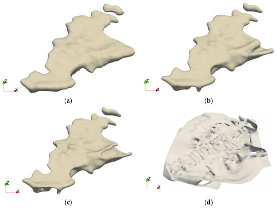
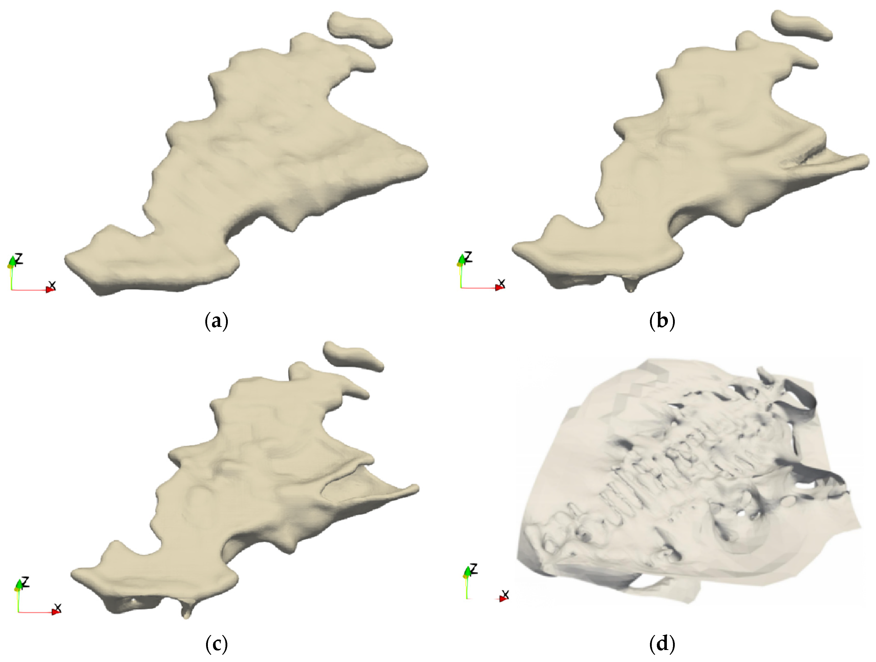
Let represent a set of unit directional vectors, and let be the implicit scalar function to be solved, defined as follows:
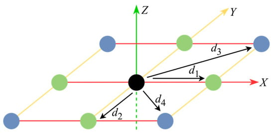
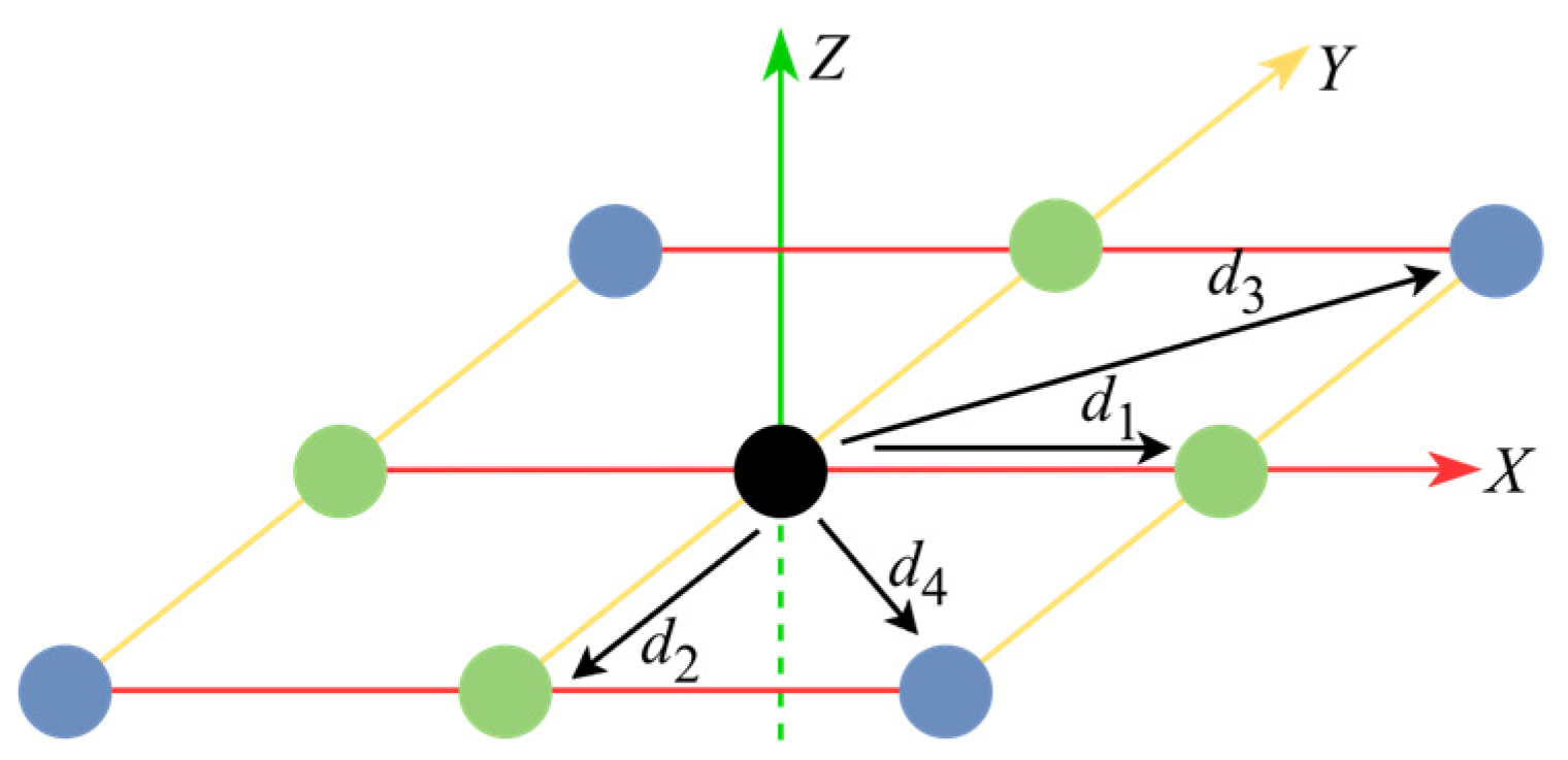
where denotes the second-order directional derivative along the direction . As shown in Figure 1, the direction set in two dimensions (2D) includes axial and face-diagonal directions (and body-diagonal directions in 3D), thereby constituting a complete second-order derivative space [33]. Under a uniform grid structure, the second-order derivatives along the direction of and the mixed derivatives along the two orthogonal directions and can be approximated using standard second-order FDs. Assuming that and denote the spacing between adjacent grid nodes in the and directions, respectively, at node , we have:
Figure 1.
Notion of set of directional vectors in two dimensions [33].
Without introducing boundary conditions, for a given set of sampling points (), a stable implicit scalar field can be constructed by seeking a solution that simultaneously satisfies the interpolation constraints and the structural smoothness requirements. Specifically, the interpolation constraints () are formulated to ensure that the scalar field passes through the sampled data, while the hybrid regularization operator () is employed as a governing PDE to maintain geometric continuity.
By discretizing these constraints on the grid, the problem is converted into an overdetermined linear system. The interpolation constraints form the upper block (), mapping the grid nodes to the sampled values (). Meanwhile, the discretization of the regularization operator (Equations (3) and (4)) forms the penalty block (), which forces the field to satisfy the smoothness criteria. Consequently, the resulting discrete linear system in block matrix form is expressed as:
Here, denotes the vector of function values at grid points. Evidently, the total number of nodes grows cubically as the resolution increases. When applied to large-scale, highly non-uniformly distributed orebody sampling data, memory and computational costs rapidly become restrictive bottlenecks.
3. Adaptive FD Method
3.1. Overall Workflow
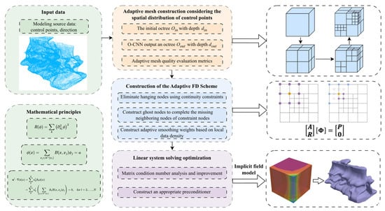
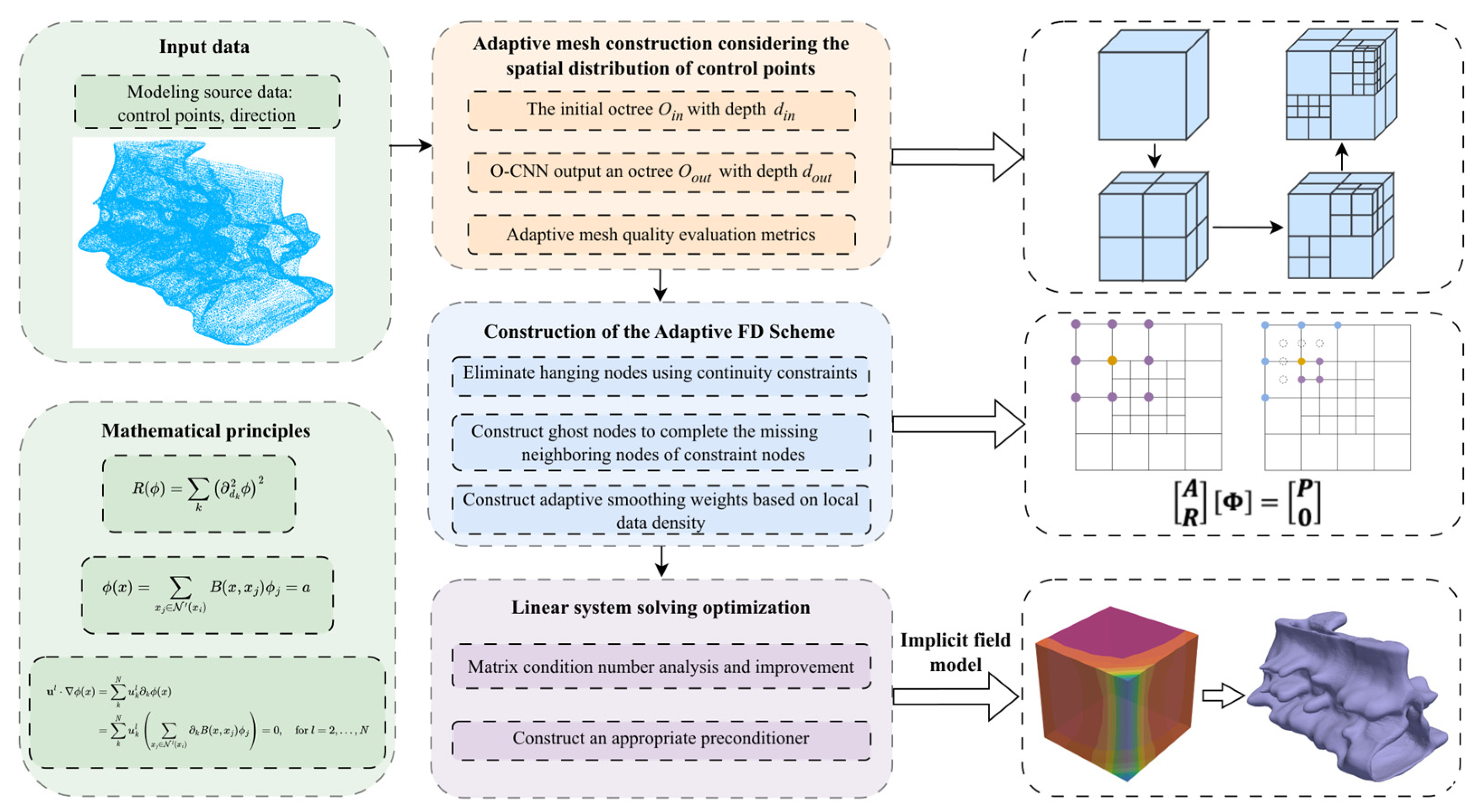
Targeting large-scale and non-uniformly distributed control point data, AdaFDI partitions the computational domain into a hierarchical adaptive octree mesh and designs an adaptive FD scheme upon this structure, thereby drastically reducing the computational scale and costs. Figure 2 shows the workflow of the proposed method, comprising four primary steps:
Figure 2.
Workflow illustration of Adaptive FD method for constructing 3D orebody model.
- (1)
- Based on the control point distribution, an initial octree with depth was constructed. By introducing the octree-based CNN (O-CNN) framework [36], data points with similar local geometric features were merged into the same finest-level cells, yielding an optimal adaptive octree mesh accounting for spatial similarity while meeting total mesh count limits.
- (2)
- Targeting special nodes within the adaptive mesh, variant FD schemes satisfying continuity constraints were constructed to complete the discretization of the regularization operator.
- (3)
- Based on the structural characteristics of the constructed linear system, an appropriate numerical solving strategy was selected.
- (4)
- The final orebody model was obtained by extracting the isosurface from the solved implicit field.
3.2. Adaptive Mesh Construction
The adaptive octree mesh used for numerical computation must satisfy a compatibility condition, ensuring that the depth difference between adjacent meshes does not exceed 1. Octree local subdivision accounting for control point distribution generally employs two approaches: a priori geometric subdivision based on sampling point information, and dynamic subdivision based on a posteriori iterative error indicators [35,37,38]. Although the latter theoretically provides optimal convergence accuracy, in large-scale, static data scenarios, such as orebody modeling, frequent global error estimation and matrix reconstruction lead to surging computational costs. In contrast, the a priori geometric subdivision strategy is far more efficient.
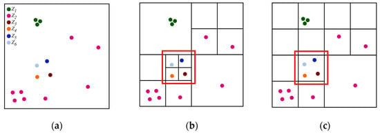
Adaptive meshing requires designing a subdivision strategy for scenarios where multiple control points fall into the same cell, ensuring that points with significant structural differences are ultimately distributed into different cells. Figure 3 illustrates two scenarios of adaptive mesh partitioning based on control points, where six types of control points with different attribute values are distributed in the mesh space. The method shown in Figure 3c refines the mesh solely based on geometric positions, given a specified depth () and maximum total mesh count (). At maximum depth, the mesh scale may be insufficient to resolve the data heterogeneity within the cell (red box, Figure 3c), causing a loss of control point information validity during the discretization stage. Furthermore, attribute differences are excluded, and cells containing three control points with identical attributes (green points, Figure 3c) are over-refined, adding redundant nodes that contribute nothing to accuracy enhancement. In contrast, Figure 3b introduces an identification mechanism for the feature consistency among control points, aggregating meshes for points with similar features to prevent over-refinement. Concurrently, under the same constraint, it ensures that finest-level cells reflect local data attributes and structural features more precisely (red box, Figure 3b). We utilized Equation (10), which characterizes local similarity, to describe this refinement property.
Figure 3.
Adaptive mesh subdivision strategy. (a) Control point data distribution with different attributes; (b) mesh refinement based on control point distribution; (c) mesh refinement strategy considering only geometric positions.
However, when the octree depth is substantial, accounting for the local similarity features of control points requires performing covariance matrix decomposition, sorting, and filtering leaf by leaf, which prevents efficient computation. Therefore, we introduced the feature-driven O-CNN framework [36] as a data-driven geometric subdivision and grouping mechanism to construct a geometry-aware octree mesh.
Unlike neural implicit reconstruction approaches, the O-CNN framework in this study is not used to directly predict implicit scalar fields or orebody boundaries. Instead, it serves only as a geometry-aware, adaptive octree partitioning strategy prior to FD discretization.
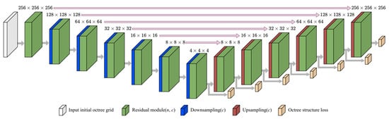
Figure 4 illustrates the architecture of the adopted O-CNN framework. The model takes an initial octree of depth , constructed from the spatial distribution of raw data points, as input. During the encoder stage (corresponding to the downsampling process in the original O-CNN terminology), local geometric features are progressively aggregated from finer octree levels to coarser levels, enabling the network to capture hierarchical structural characteristics of the point distribution. Subsequently, during the decoder stage (upsampling process), the aggregated feature information is propagated back from coarse levels to finer octree cells to predict adaptive subdivision patterns.
Figure 4.
O-CNN-based hierarchical feature aggregation and adaptive octree subdivision process for geometry-aware mesh construction. (Adapted from [36]).
The encoder–decoder process of the O-CNN framework can be regarded as an efficient approximation of the original leaf-wise local similarity analysis strategy proposed in this study. In conventional adaptive octree subdivision, covariance decomposition, feature sorting, and filtering operations must be repeatedly performed for individual leaf cells to evaluate the local structural similarity of control points, resulting in rapidly increasing computational costs as the octree depth increases. By contrast, the hierarchical feature aggregation mechanism of the O-CNN enables the efficient multi-scale extraction of neighboring geometric distribution features across octree levels, thereby improving the adaptive subdivision efficiency while preserving local structural consistency under sparse and non-uniform sampling conditions.
To ensure that the O-CNN framework robustly learned the diverse geometric features of orebody distributions (e.g., varying point densities and geometric anisotropy), we combined the public O-CNN benchmark dataset with a custom domain-specific synthetic geological dataset during the training phase. Due to the limited sample size of available public orebody models, we utilized standard models from Leapfrog software tutorials [39] as geometric prototypes. To construct a comprehensive and highly diverse training dataset, we applied rigorous data augmentation techniques to the points extracted from these prototypes, including random anisotropic scaling, rotation, local spatial deformation, and simulated variable-density drillhole resampling.
Furthermore, to provide accurate geometric supervision during network training, the high-resolution, watertight implicit meshes generated by Leapfrog’s FastRBF algorithm were employed as the ground truth. By calculating the structure and normal losses against these baseline Leapfrog models, the O-CNN was explicitly trained to predict optimal, geometry-aware adaptive octree subdivisions even under sparse and non-uniform sampling conditions. The trained O-CNN framework ultimately outputs an adaptive octree mesh of depth driven by local geometric features.
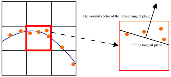
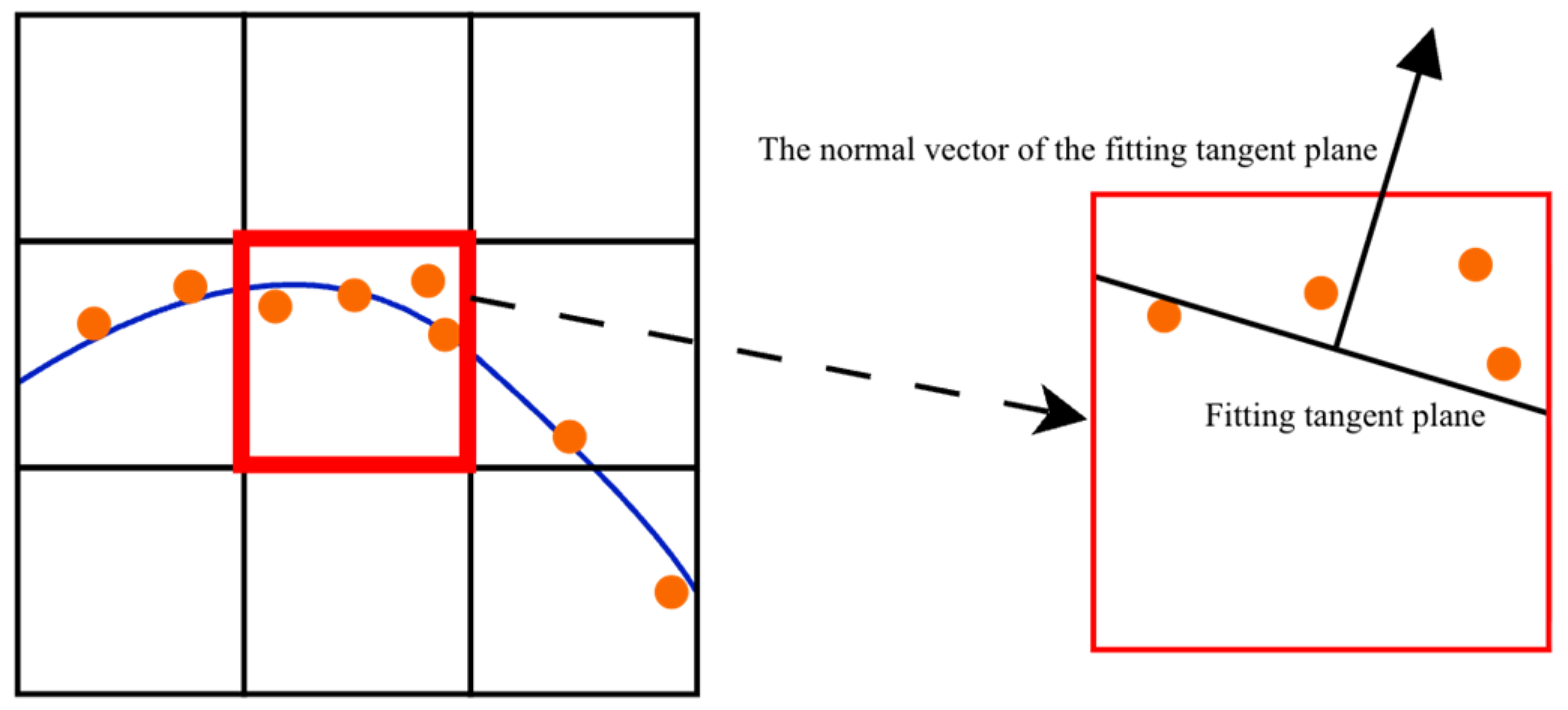
To quantitatively evaluate the local structural consistency of control points within the adaptive octree mesh, a local coplanarity deviation value () was defined in each finest-level non-empty cell (), based on the average point-to-plane deviation between control points and their locally fitted tangent plane. The local tangent plane was estimated using the PCA-based covariance analysis of neighboring control points rather than derived from the implicit scalar field.
Based on , two evaluation metrics for quantifying the adaptive meshing quality were further proposed: the average coplanarity () and maximum coplanarity error (). These metrics characterize the degree of local geometric inconsistency between control points and the fitted tangent plane within each octree cell, as shown in Figure 5.
Figure 5.
Schematic representation of average coplanarity error for locally similar control points. The orange points represent the control point data, and the blue curve represents the fitted curve.
Let the set of finest-level non-empty cells be . The set of data points contained in the -th cell () is:
Let the neighborhood cell () set of the -th cell be , and the point set contained within be
The centroid () of the point set () is:
The covariance matrix constructed based on the centroid () is:
Let be the minimum eigenvalue of and its corresponding unit eigenvector () be regarded as the normal vector of the optimal fitting plane within . The calculation formula for the coplanarity deviation value () of control points within the cell () is defined as:
where is the corresponding plane offset term, expressed as:
Based on Equation (10), the average coplanarity error () and maximum coplanarity error () are defined respectively as:
3.3. Construction of Adaptive FD Scheme
3.3.1. Handling Method for Hanging Nodes
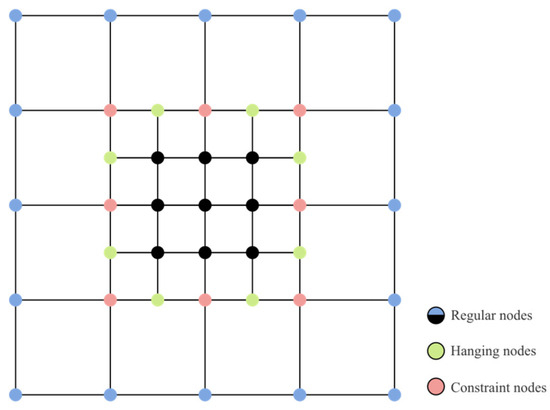
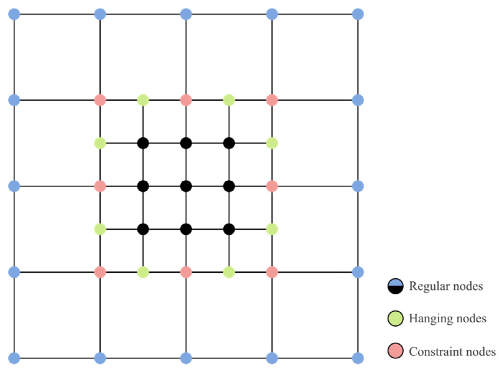
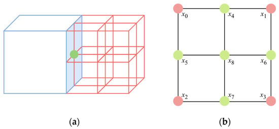
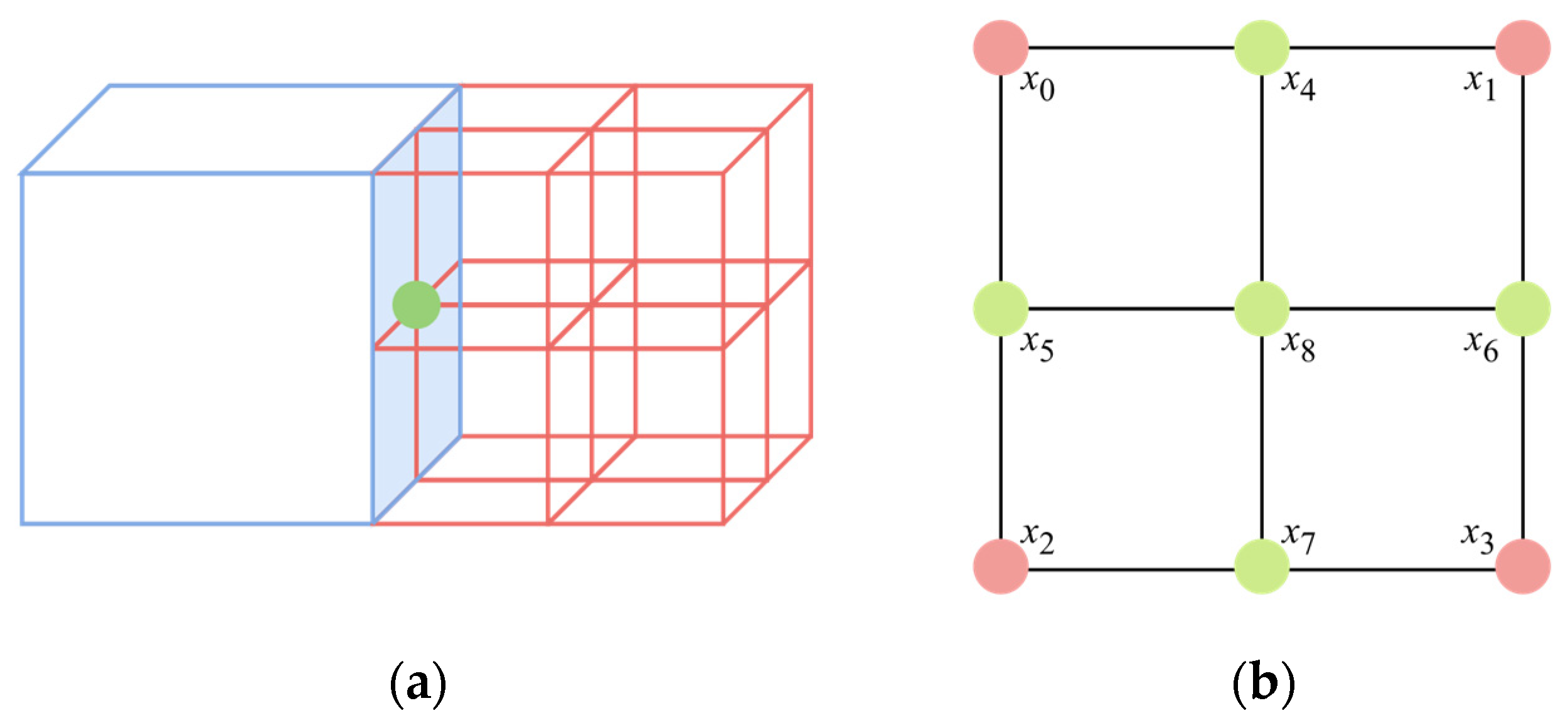
To construct a linear system on the adaptive octree mesh consistent with the original regularization operator, we modified the uniform-grid-based FD schemes in Equations (3) and (4), proposing an adaptive FD method. Figure 6 displays a local 2D adaptive mesh containing two hierarchy levels: coarse meshes () and fine meshes (). Nodes associated with only a single mesh level were defined as regular nodes (e.g., the blue nodes associated only with the coarse mesh () and the black nodes associated only with the fine mesh () in Figure 6). The difference schemes for such nodes required no modification. Green nodes located at the refinement boundary and associated exclusively with the fine mesh () were defined as hanging nodes. In 3D space, face-center hanging nodes also exist at the refinement boundary (the blue plane), as shown in Figure 7a.
Figure 6.
Local two-dimensional (2D) adaptive mesh including two refinement levels.
Figure 7.
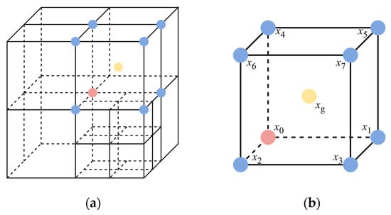
Hanging nodes. (a) Hanging nodes at face-center in three-dimensional (3D) space; (b) continuity constraint example for hanging nodes.
To ensure the continuity of the numerical solution, continuity constraints were applied to hanging nodes to express hanging nodes as linear combinations of adjacent regular nodes, thereby eliminating them at the algebraic level. Taking Figure 7b as an example, midpoints on lines were constrained using , , and were similarly processed, and midpoints on faces were constrained as . All constraint information was recursively constructed into a constraint matrix (), ensuring that the linear system transformed via . This matrix no longer contained the degrees of freedom corresponding to hanging nodes. This achieved the goal of eliminating hanging nodes through algebraic constraints.
3.3.2. Handling Method for Constraint Nodes
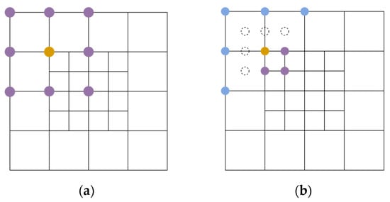
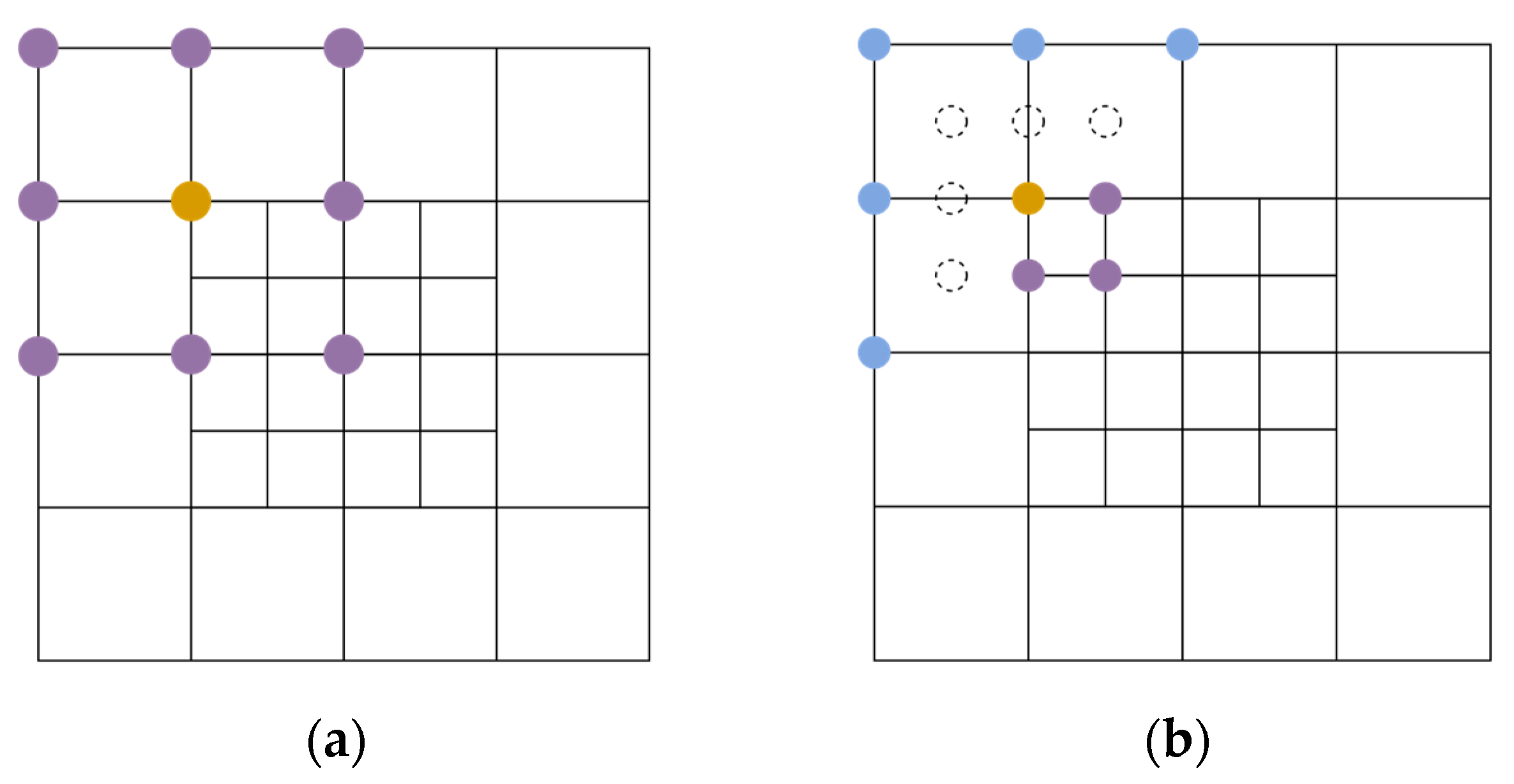
Nodes located at the mesh refinement boundary and associated simultaneously with both mesh levels were defined as constraint nodes (e.g., the red nodes in Figure 6). Suppose the mesh step sizes and direction sets for the coarse meshes () and fine meshes () were , and , , respectively. Because constraint nodes were associated with both levels, two choices ( and ) of step size were available when calculating second-order derivatives. The calculation method dictated that for any direction set, if a neighboring point was missing in the difference scheme, a ghost node (virtual node) was introduced to complete the scheme, and its degrees of freedom were eliminated using the aforementioned continuity constraint method. As shown in Figure 8a, the adjacent points for the direction set corresponding to the coarse step size () are complete; however, for the direction set corresponding to the fine step size () in Figure 8b, some adjacent points are missing in the coarse mesh space. Here, corresponding ghost nodes are added to perfect the difference scheme.
Figure 8.
Neighboring nodes corresponding to direction set with different computational step sizes. (a) Neighbors corresponding to coarse grid step (): computational node (orange) and its computational neighbors (purple); (b) neighbors for fine grid step () and added ghost nodes: computational node (orange), computational neighbors (purple), extended computational neighbors (blue) and ghost nodes (dashed circles).
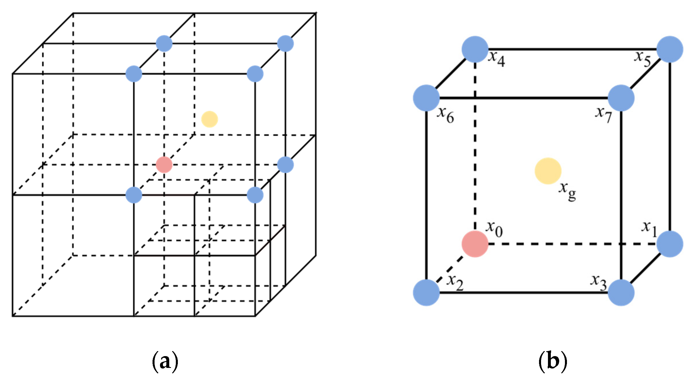
Compared with hanging nodes, ghost nodes involve an additional cube-center constraint, as shown in Figure 9a. When calculating along the body-diagonal directions of points , the ghost node at the cube center (Figure 9b) must be supplemented and constrained using . The calculation results for different step sizes are comparatively discussed in Section 5.2.
Figure 9.
Ghost nodes at cube center. (a) Ghost node distribution in three dimensions; (b) constraint example for ghost node at cube center.
3.3.3. Adaptive Smoothing Weight Method
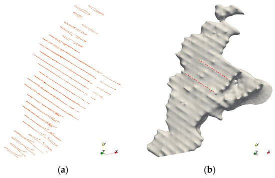
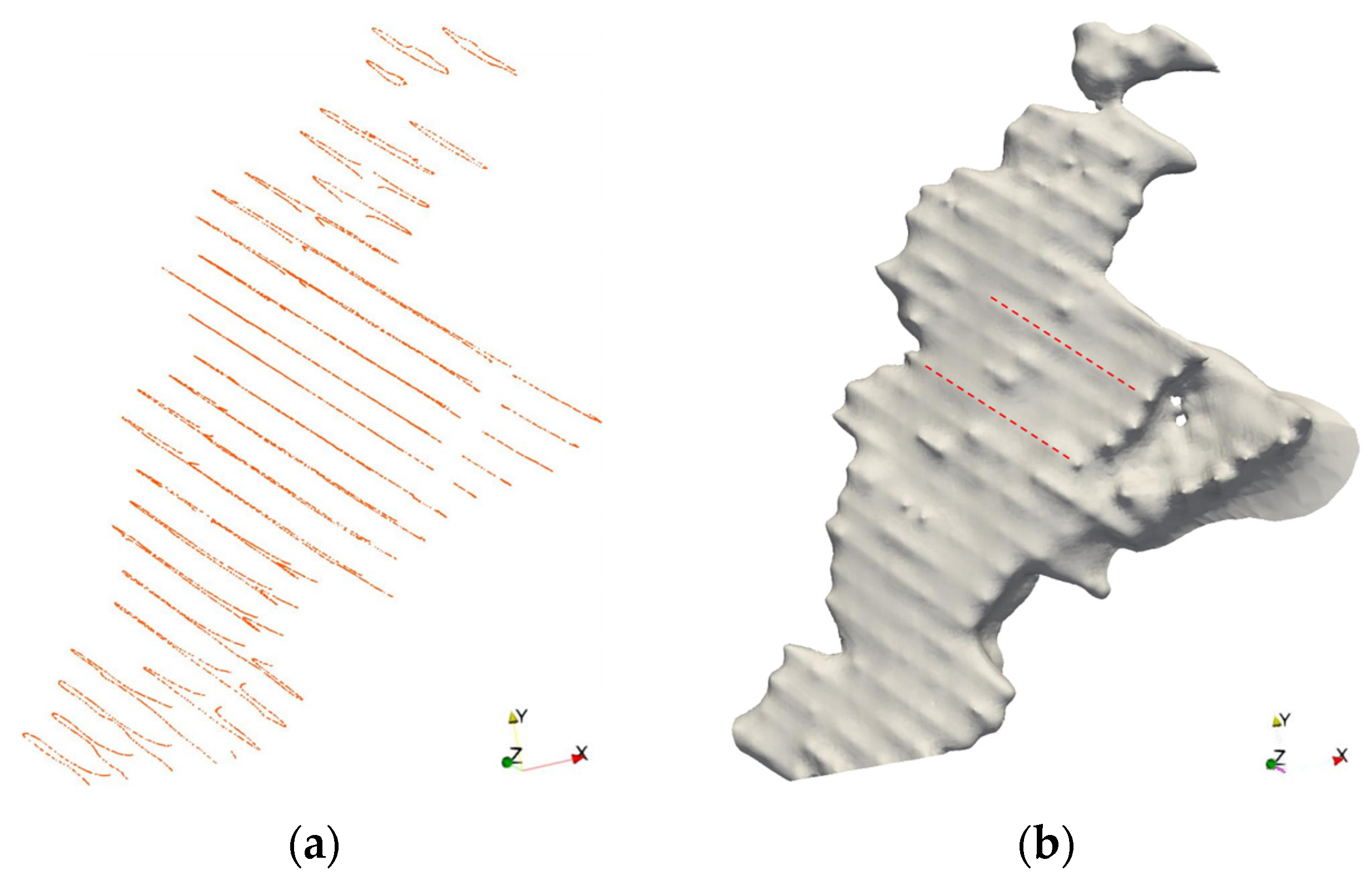
The strategies detailed above ensure the constructability and algebraic consistency of the adaptive FD scheme. However, in scenarios where data points are distributed in a nearly parallel manner with large spacing (Figure 10a), the regularization operator () introduces anisotropy within the FD discretization framework. Consequently, strong constraints in data-dense regions cannot diffuse evenly, while blank regions governed primarily by smoothing terms tend to construct planes with minimal curvature. This discrepancy across different regions causes “ridge-like” surface artifacts extending along the data distribution direction, as shown in Figure 10b.
Figure 10.
Numerical artifacts in sparse data. (a) Source data distribution pattern; (b) numerical artifacts along direction of data distribution in model results (red dashed line).
To address this, we propose an adaptive smoothing weight method based on local data density. For each finest-level non-empty cell (), its corresponding smoothing weight is defined based on the number of control points () within it:
where is the average number of control points in the finest-level cell (), is a tuning coefficient, and is a truncation parameter to prevent over-smoothing. This method dynamically strengthens the smoothing constraints of the regularization term in data-dense regions, thereby suppressing numerical artifacts along the data distribution direction. As a local weight parameter, this method does not alter the structural form of the operator, maintaining the symmetry and positive definiteness of the overall linear system.
4. Linear System Solving Optimization
4.1. Matrix Condition Number Analysis
The system of linear equations in Equation (5) is typically solved using iterative methods. The convergence rate of iterative methods is heavily influenced by the spectral properties of the system matrix, particularly the condition number [40]. The condition number characterizes the degree of ill-conditioning of the system: a high condition number causes a slow reduction in computational residuals, substantially increasing the number of required iterations. Considering the diagonally dominant nature of the matrix (), we employed a diagonal-scaled condition number indicator as an approximate substitute for the matrix condition number, defined as:
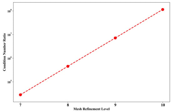
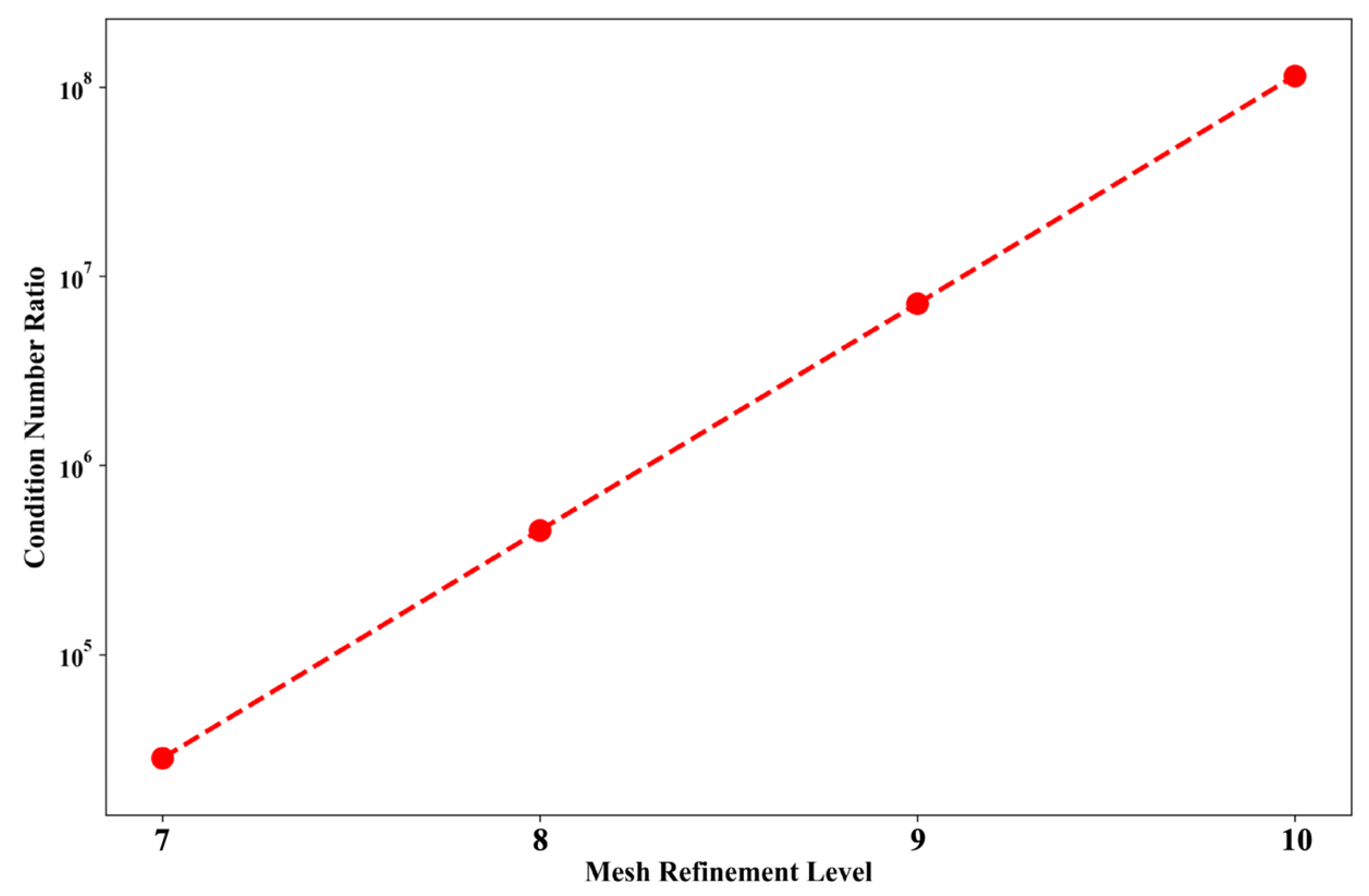
where and represent the absolute values of the maximum and minimum diagonal elements in the matrix (), respectively. In the FD discrete structure, the coefficients in the matrix () are generally strongly correlated with the mesh computational step size. Diagonal terms corresponding to fine-mesh nodes tend to possess larger numerical values, resulting in an extremely unbalanced overall matrix scale. Continuous mesh refinement further exacerbates the ill-conditioning of the linear system. Figure 11 illustrates the corresponding values of at different mesh refinement depths. When the refinement depth reaches 10 levels, reaches the order of . This phenomenon severely impairs the solving efficiency, leading to sluggish overall convergence.
Figure 11.
Numerical values of condition number indicator () versus level of mesh refinement.
4.2. Matrix Condition Number Improvement
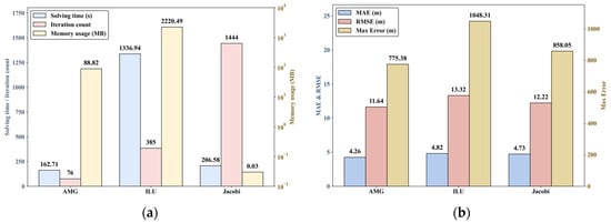
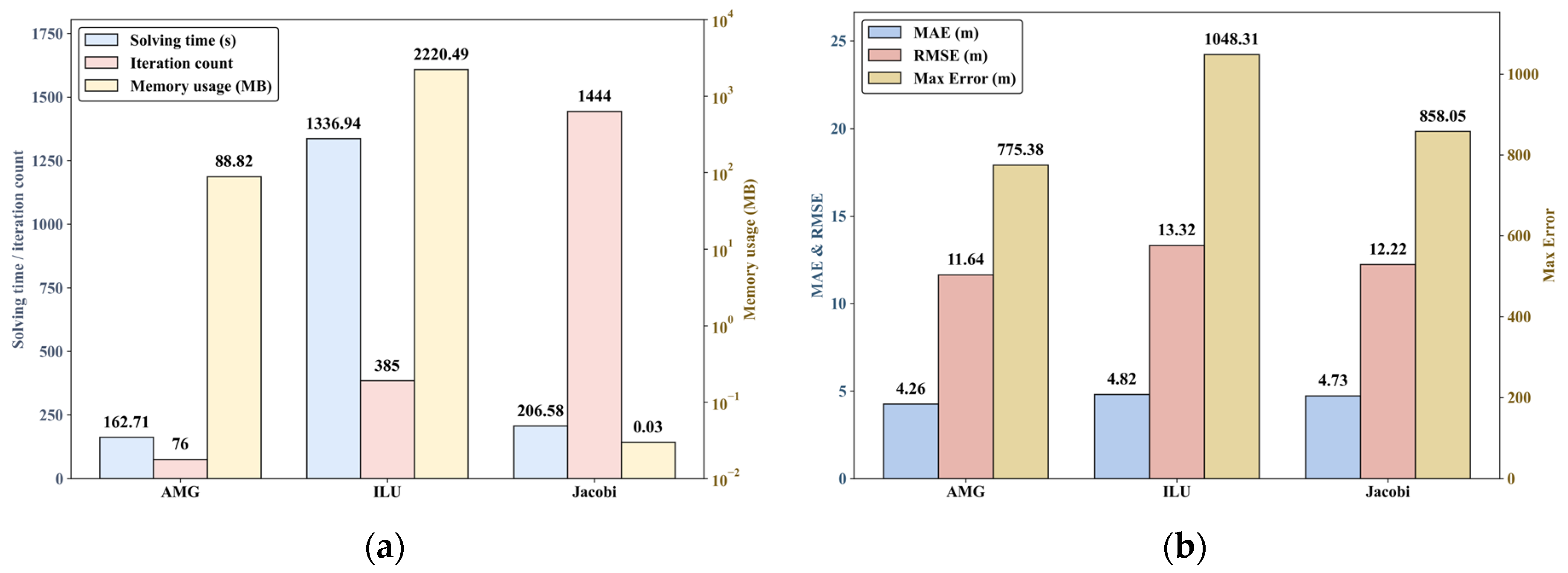
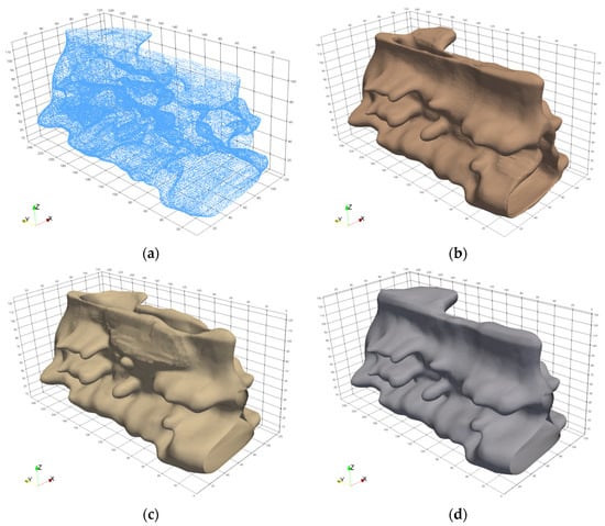
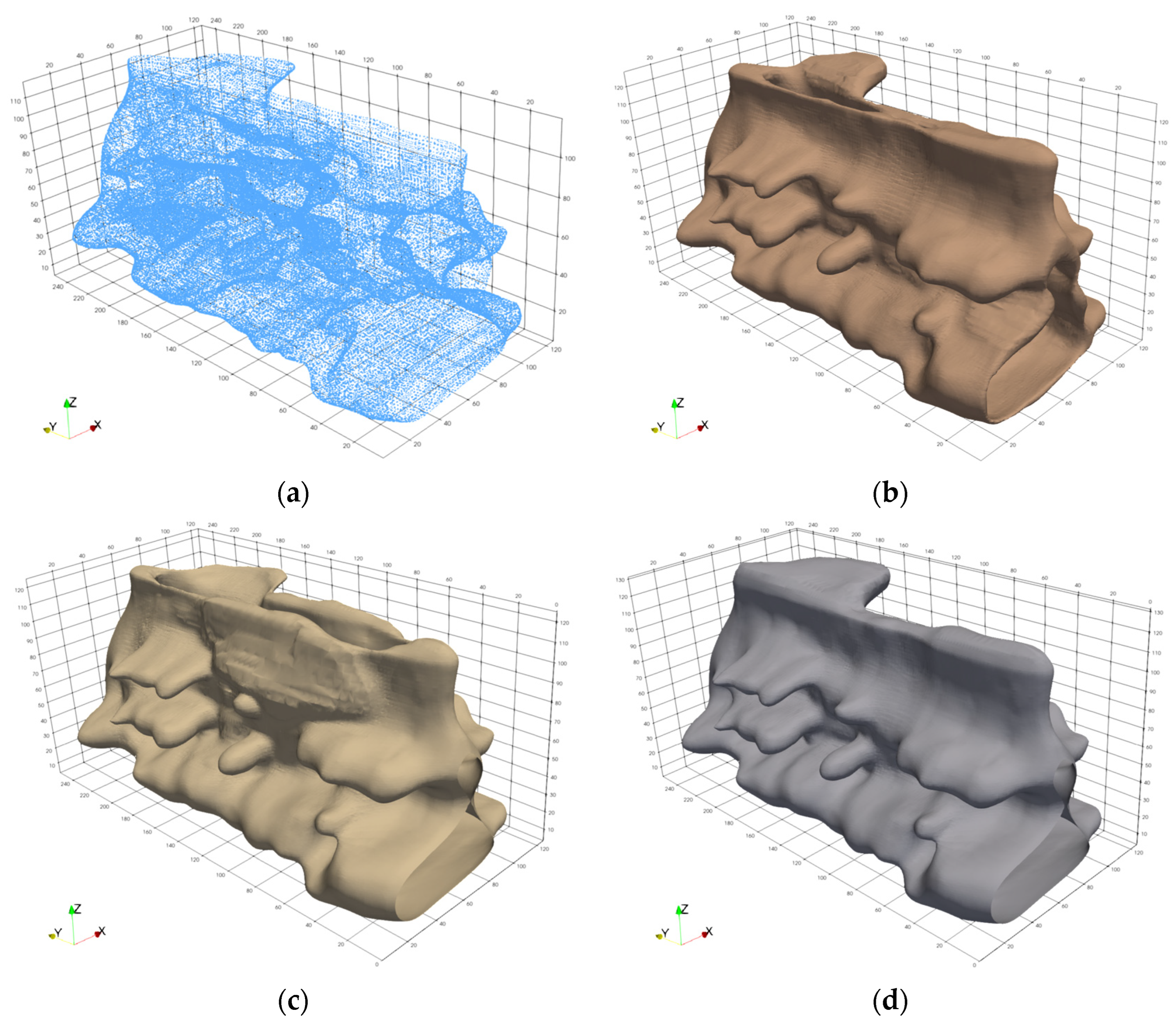
To improve the spectral properties of the system matrix () and reduce the condition number (), preconditioning of the linear system is required. The core concept is to construct an effective preconditioner () such that the transformed system () exhibits a superior numerical distribution pattern (i.e., a lower condition number indicator) (). This study comparatively tested three preconditioning methods: Jacobi, Incomplete LU (ILU) factorization, and Algebraic Multigrid (AMG). Under the maximum mesh refinement depth of , the performance and modeling results of the three preconditioners are shown in Figure 12 and Figure 13, respectively.
Figure 12.
Performance comparison of three preconditioners under test. (a) Comparison of solving time, iteration count, and memory usage; (b) comparison of maximum absolute error (Max Error), mean absolute error (MAE), and root-mean-square error (RMSE).
Figure 13.
Comparison of test models for three preconditioners. (a) Source data distribution pattern; (b) model results with AMG preconditioning; (c) model results with ILU preconditioning; (d) model results with Jacobi preconditioning.
The Jacobi preconditioner was constructed as , which balances the weight of each equation in the original system through diagonal scaling, thereby reducing the matrix condition number [41]. Although this preconditioner was constructed easily with minimal memory overhead, it excludes the off-diagonal elements of the matrix, leading to a substantial increase in solving iterations.
The ILU preconditioner captures the global coupling structure of the matrix through approximate factorization () while controlling the computational scale by dropping fill-ins, which improves the system’s spectral properties to some extent [42]. However, as the problem scale grows, the number of fill-ins increases rapidly, making it difficult to control memory consumption and construction costs. Furthermore, due to the non-uniform coupling characteristics between nodes of different scales in the adaptive mesh, the parameters of its dropping strategy are highly sensitive, making it difficult to maintain stable preconditioning quality as the mesh scale varies.
The AMG preconditioner automatically identifies strongly connected directions among computational nodes. Because it demonstrates an optimal computational performance and optimal modeling effects, it is the most suitable preconditioner for adaptive mesh structures. As shown in Figure 12b, AMG also yields the best quantitative quality (e.g., the lowest RMSE and Max Error).
5. Numerical Experiments
In this section, two datasets were utilized to test orebody boundary modeling. Data1 is a large-scale, densely distributed dataset, whereas Data2 is a smaller-scale dataset distributed along survey lines. The detailed modeling results of both datasets and the original source data are provided in the Supplementary Materials. Information regarding both datasets is detailed in Table 1. Four scenarios with maximum mesh refinement depths of 7, 8, 9, and 10 levels were tested to analyze the overall performance of the adaptive FD method, including the construction quality of the adaptive mesh, numerical solution accuracy, and solving performance. The testing environment was a 64-bit Windows 11 OS (Microsoft Corporation, Redmond, WA, USA) with a 12th Gen Intel® Core™ i7-12700H processor (Intel Corporation, Santa Clara, CA, USA) and 16 GB of RAM. In all tests, the relative tolerance was set to , and the maximum number of iterations was 1000. In Equation (14), the tuning coefficient () and initial smoothing coefficient () were both set to 1, with . Modeling results from Leapfrog software [43] and a uniform-grid FDM with a scale of were used as baseline standards for comparison.
Table 1.
Test dataset information.
5.1. Comprehensive Performance Evaluation
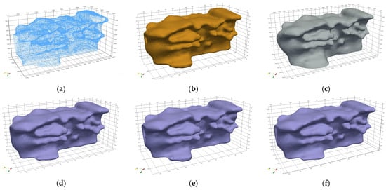
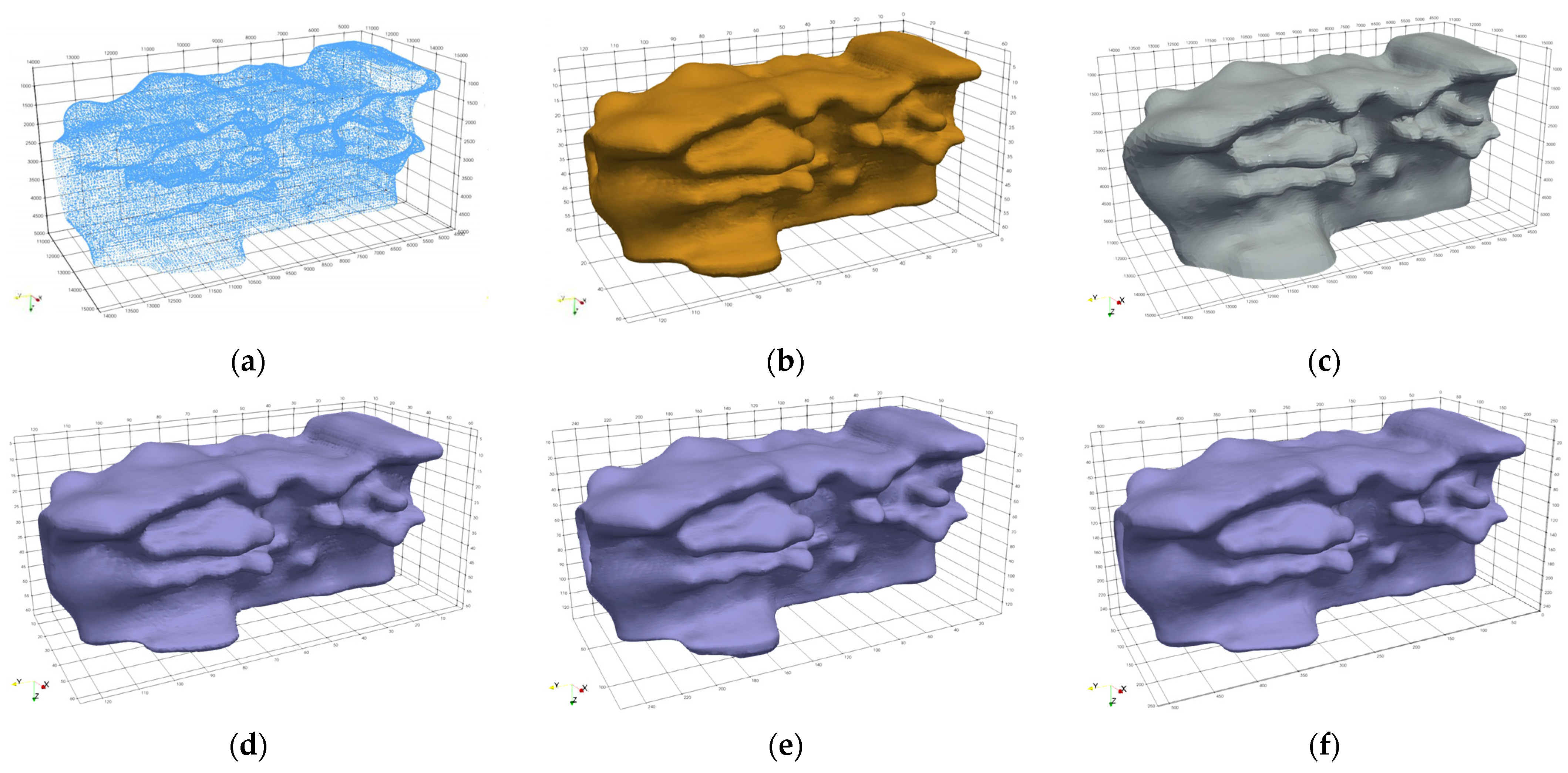
Data1 was used to verify the ability of the proposed method to handle large-scale data. The proposed adaptive FDM (AdaFDI) successfully completed model construction under three mesh resolutions: 60 m (), 30 m (), and 15 m (). For comparison, due to memory limitations, the uniform-grid FDM could only be computed at a maximum resolution of 60 m (). Meanwhile, modeling results from Leapfrog (based on the FastRBF method) served as the meshless baseline. Comparisons of the modeling results and performances among the three methods are shown in Figure 14 and Table 2, respectively.
Figure 14.
Comparison of Data1 test results for three methods. (a) Source data distribution pattern; (b) uniform-grid FDM model results; (c) LeapFrog model results; (d) AdaFDI results (60 m resolution and ); (e) AdaFDI results (30 m resolution and ); (f) AdaFDI results (15 m resolution and ).
Table 2.
Test results of three methods on Data1.
As observed in Table 2, the RBF method encountered a performance bottleneck of excessive modeling time during large-scale data processing. In contrast, the proposed AdaFDI method exhibited several advantages: (1) it achieved high-precision modeling with a resolution of up to 15 m; (2) the modeling morphologies at 15 and 30 m resolutions were highly consistent with the Leapfrog’s result under 30 m sampling while yielding superior fitting errors; and (3) the modeling times for the proposed method across all resolutions were significantly shorter than those of Leapfrog.
The robustness was further validated on the sparse Data2 (source distribution shown in Figure 10a), and modeling was completed at 80 m (), 40 m (), and 20 m () resolutions, which were compared with Leapfrog’s results at a 20 m resolution (Figure 15 and Table 3).
Figure 15.
Comparison of Data2 test results for two methods. (a) AdaFDI results (80 m resolution and ); (b) AdaFDI results (40 m resolution and ); (c) AdaFDI results (20 m resolution and ); (d) LeapFrog results (20 m resolution).
Table 3.
Test results of two methods on Data2.
Under sparse and uneven data distribution, the two methods exhibited divergent characteristics. As indicated in Table 3, the proposed AdaFDI method outperformed the RBF method in both computational efficiency and fitting accuracy. The fitting effectiveness of the RBF method heavily depended on the data distribution within its local search radius. In data-sparse regions, limited local samples made the model prone to morphological discontinuities and internal voids (Figure 15d), resulting in poor overall structural integrity. Despite its strong boundary extrapolation capability, this localized computation strategy sacrificed model integrity, making it difficult to guarantee global fitting quality. Conversely, the proposed AdaFDI method employed a global strategy. By systematically adjusting the coupling coefficients between nodes via the constraint matrix, it strengthened the constraints of control points on the overall morphology. Consequently, it generated more continuous and closed orebody models under sparse data conditions, demonstrating superior modeling stability.
The two evaluation metrics for the quality of adaptive meshes, the average coplanarity () and maximum coplanarity error (), constructed under different refinement scales for both datasets are presented in Table 4.
Table 4.
Mesh quality evaluation metrics for two sets of data.
5.2. Strategy Analysis of Different Computational Step Sizes for Constraint Nodes
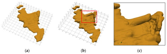
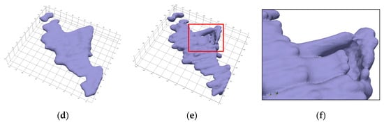
To evaluate the two computational step size strategies for constraint nodes discussed in Section 3.3.2, tests were conducted on Data1 and Data2 at maximum refinement depths of and . Performance comparisons are listed in Table 5, and the modeling results for Data2 are shown in Figure 16.
Table 5.
Data2 test results for two calculation step sizes.
Figure 16.
Models of Data2 based on different step strategies. (a) Model results with coarse grid step size () and ; (b) model results with coarse grid step size () and ; (c) local details within red-box region; (d) model results with fine grid step size () and ; (e) model results with fine grid step size () and ; (f) local details within red-box region.
Results indicated that both schemes possessed unique advantages under different data distribution characteristics. The fine-mesh step size scheme extended the coverage of fine-mesh nodes by adding ghost nodes, enhancing the numerical coupling between nodes across different levels. It performed excellently when handling the sparsely distributed Data2, effectively improving the overall smoothness and continuity of the model. However, this scheme increased the complexity of constructing the linear system. When processing massive, dense datasets such as Data1, it led to a significant surge in the memory consumption and solving time at and greater depths.
The coarse-mesh step size scheme offers a simpler and more direct linear system construction. It displayed obvious advantages when processing Data1, effectively reducing the computational overhead while ensuring model accuracy. However, when handling the sparse Data2, this simplified construction caused partial decoupling between constraint and internal fine-mesh nodes, slightly degrading the model smoothness.
5.3. Numerical Artifacts in Sparse Data
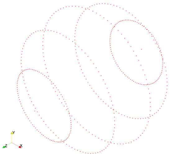
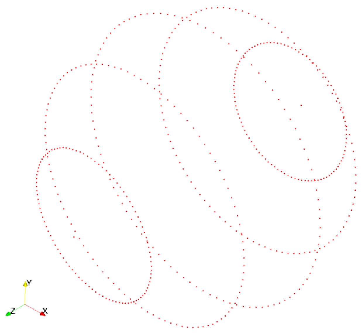
To rigorously evaluate the adaptive smoothing strategy and isolate the artifact generation mechanism from the uncertainties inherent in real geological boundaries, we first designed a synthetic sphere benchmark with controlled sparse sampling. The target was an ideal sphere with a radius of 1000. To simulate the highly anisotropic and sparse data distribution typical of parallel exploration lines, the control points were sparsely sampled along five latitudinal bands (−60°, −30°, 0°, 30°, and 60°), with 100 points uniformly distributed on each respective circular plane. Including two control points at the poles, the dataset comprises a total of 502 control points (Figure 17).
Figure 17.
Sparse spatial distribution of control points used for synthetic sphere benchmark.
To quantitatively assess the model quality, we evaluated both the RMSE for the fitting accuracy and the sphericity () for the global morphological smoothness. Sphericity measures how closely a 3D object approaches the shape of a perfect sphere (), defined as:
where is the volume of the model, and is its surface area.
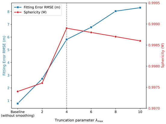
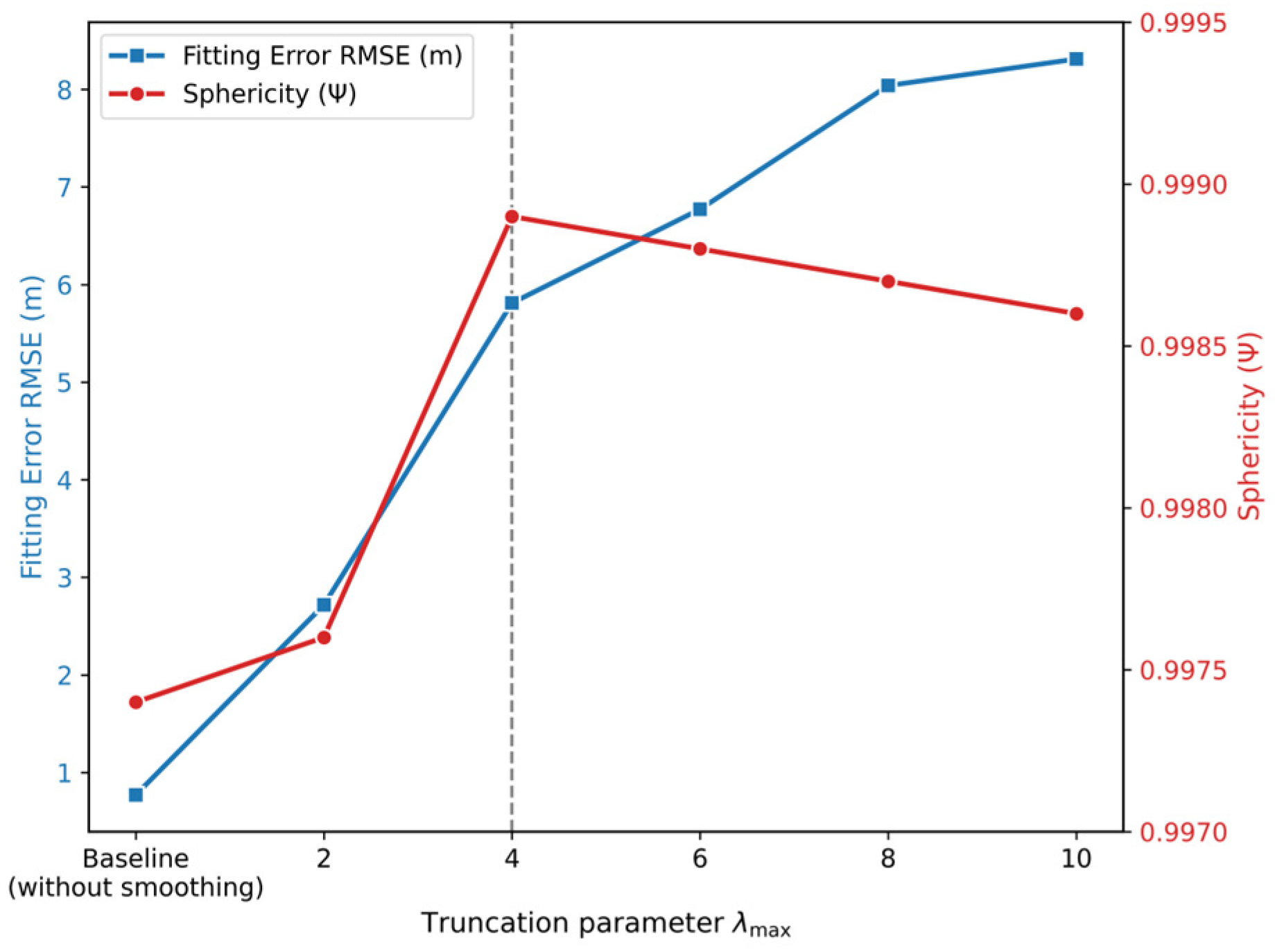
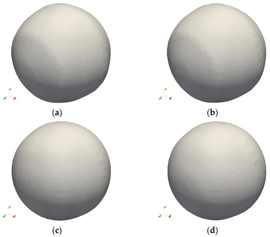
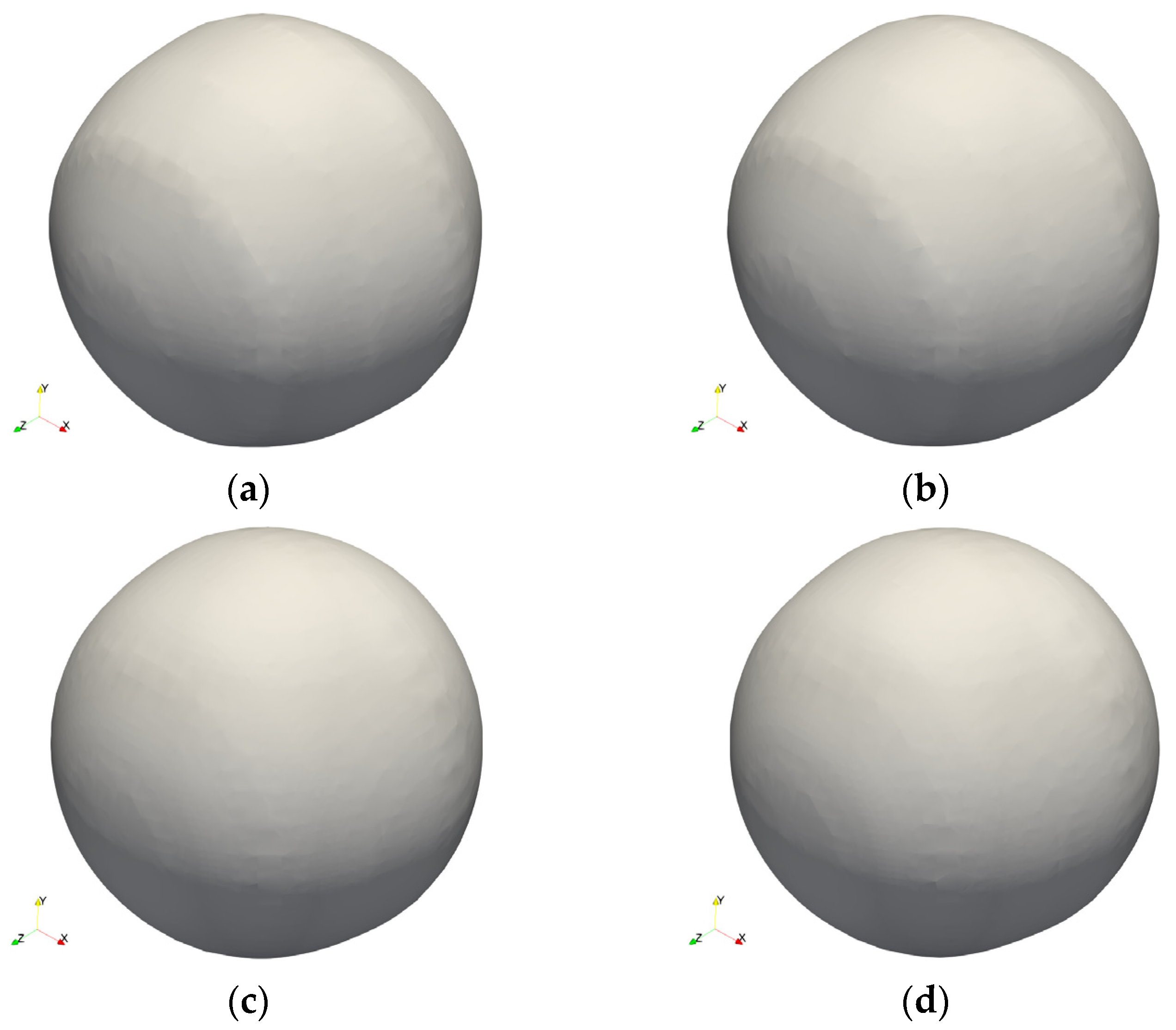
We tested six configurations of the truncation parameter (): baseline (without smoothing), 2, 4, 6, 8, and 10. The baseline model yielded the lowest RMSE (Figure 18) but exhibited pronounced “ridge-like” numerical artifacts along the latitudinal sampling bands, resulting in the lowest sphericity (Figure 19a). This confirms that the anisotropic nature of the discrete regularization operator inherently generates morphological distortions under sparse parallel constraints.
Figure 18.
Effect of truncation parameter () on fitting error RMSE and sphericity of synthetic sphere model.
Figure 19.
Comparison of synthetic sphere models under varying smoothing truncation parameters (). (a) Baseline model without smoothing; (b) model with ; (c) optimal model with ; (d) model with .
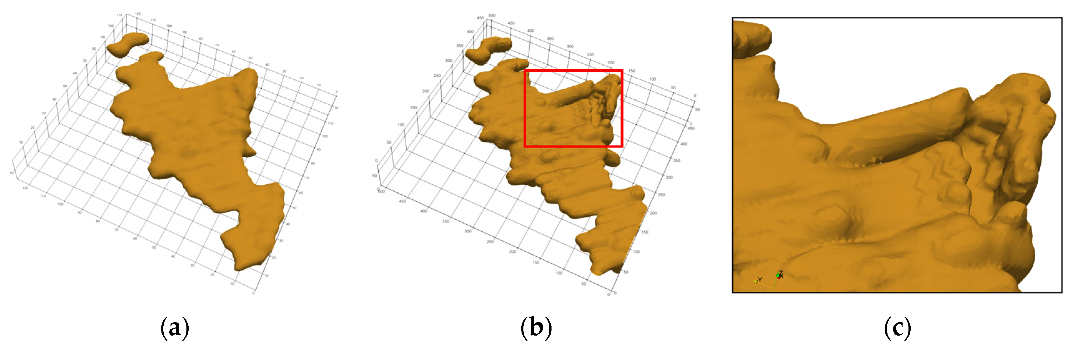
Upon introducing the adaptive smoothing weight, the numerical artifacts were visibly suppressed (Figure 19). The quantitative analysis reveals a clear “no free lunch” trade-off between geometric morphological fidelity and strict interpolation accuracy (Figure 18). As increased to 4, the model achieved its peak sphericity, effectively smoothing out the high-frequency ridges around the control point bands and restoring a smooth spherical surface (Figure 19c). At this optimal configuration, the RMSE increased to approximately 7 times that of the un-smoothed baseline model. This indicates that achieving global morphological rationality inevitably requires a controlled relaxation of local data interpolation constraints. Further increasing beyond 4 over-penalized the curvature, leading to a degradation in both the local fitting accuracy and global sphericity (Figure 19d).
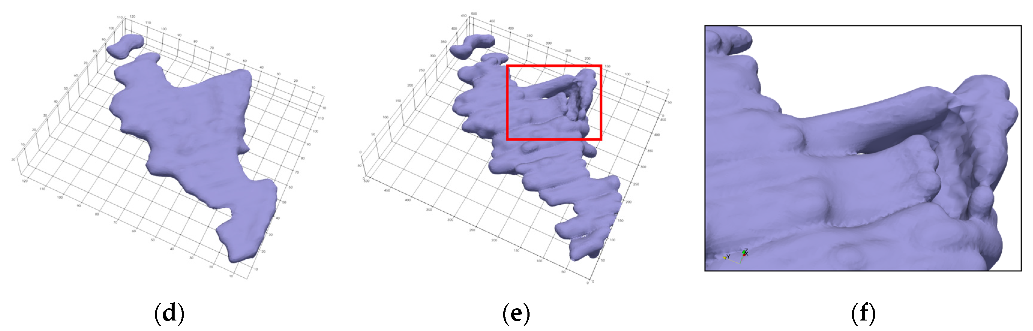
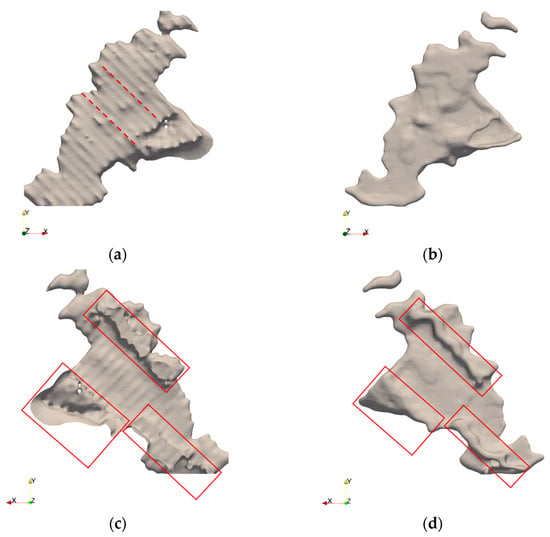
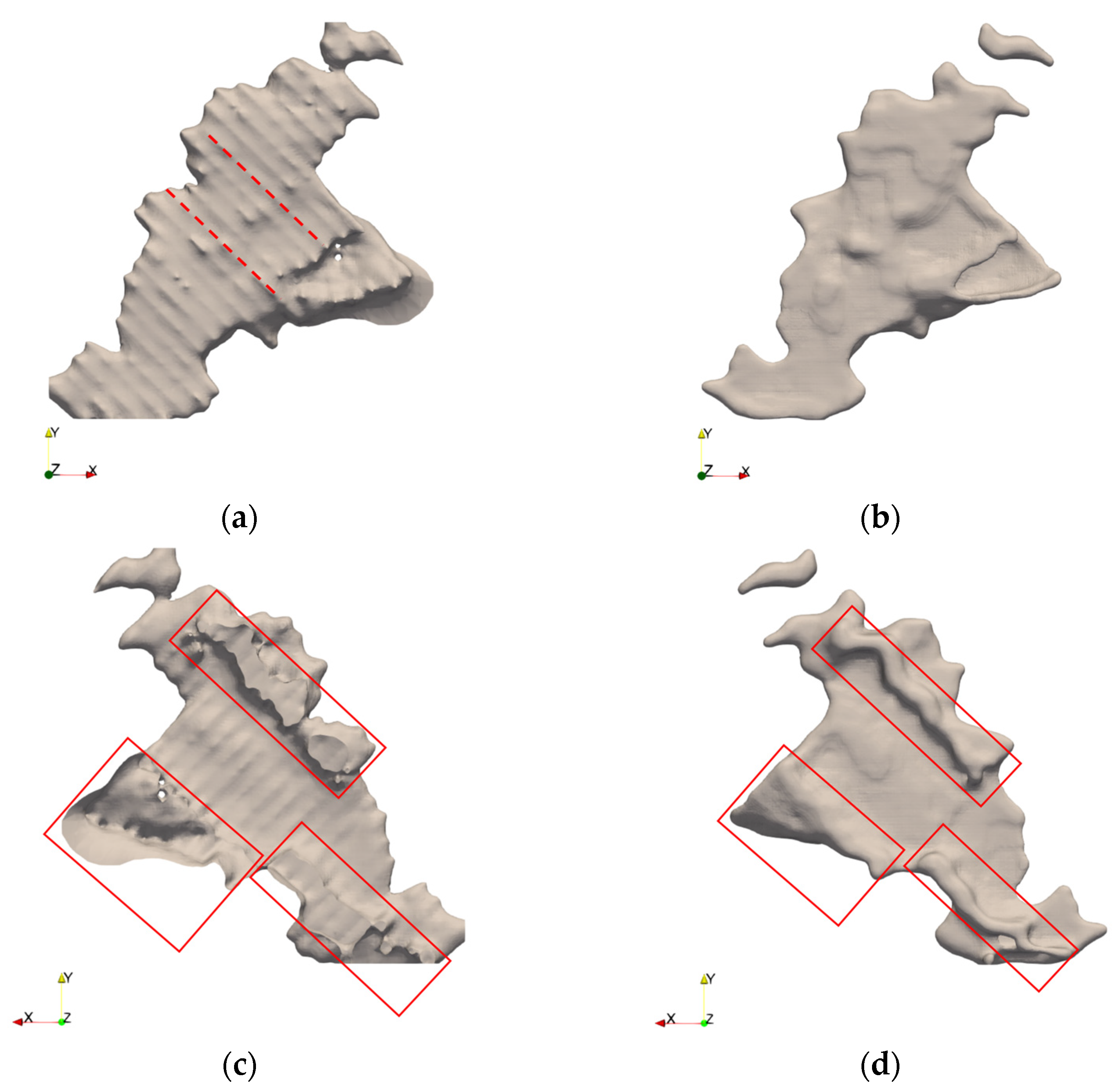
Furthermore, we evaluated the adaptive smoothing method using the real-world sparse orebody dataset, Data2 (Figure 10a). Figure 20 presents a comparison between the unoptimized and optimized models at . In this dataset, data points were densely distributed in strip-like patterns along approximately parallel directions, with extensive data-void regions existing between adjacent strips. In the unoptimized model, “ridge-like” numerical artifacts extending along the data distribution direction emerged (marked by red dashed lines in Figure 20a), and boundary continuity was disrupted within the red box in Figure 20c.
Figure 20.
Numerical artifacts and optimization effects for sparsely distributed dataset, Data2. (a) Numerical artifacts in unoptimized model; (b) smoother appearance of optimized model; (c) boundary discontinuities in unoptimized model; (d) better boundary closure of optimized model.
Following the introduction of the adaptive smoothing weight, the regularization intensity in data-dense regions was fortified, effectively balancing the relative impact of data constraints and smoothing terms across different spatial domains. The numerical artifacts extending along the data distribution direction were visibly alleviated (Figure 20b), and the overall continuity and closure of the model were enhanced (Figure 20d). These results indicate that the proposed adaptive smoothing weight strategy can effectively mitigate the numerical instability issues induced by anisotropic regularization operators under sparse data conditions.
6. Discussion and Limitations
The AdaFDI method proposed in this study implicitly constructs 3D orebody boundaries from nearly one million non-uniform control points, without relying on gradient information, by combining an adaptive octree mesh with a finite difference scheme. Numerical experiments demonstrated that this method outperformed the traditional RBF and uniform-grid finite difference methods in terms of model accuracy, computational efficiency, and memory footprint, exhibiting stronger robustness for sparsely distributed data. However, the method has several shortcomings, which are dicussed below, along with future directions for improvement:
- (1)
- Strong Coupling between Resolution and Mesh Count Limits Modeling Efficiency for Elongated Orebodies.
The proposed method employs an isotropic octree subdivision strategy, where the mesh resolution and node count have a cubic relationship. For thin-vein orebodies with extremely high aspect ratios, the generation of numerous redundant fine cells in the thickness direction leads to wasted computational resources. This subdivision mechanism, which is independent of the geometric anisotropy, struggles to efficiently process elongated geological bodies that extend predominantly in a single direction.
- (2)
- Computational Performance Remains Constrained by Mesh Scale, with Practical Limits.
Although adaptive meshing substantially reduces the total number of nodes, the performance of solving the linear system remains strongly correlated with the mesh count. Experiments described in Section 5.1 show that when the mesh count exceeds 5 million (Dmax > 10), the basic memory usage for storing the sparse matrix approaches 4 GB. Furthermore, the peak memory required during the setup and solving phases of the AMG preconditioner is significantly higher. Consequently, on a standard personal computer (e.g., 16 GB RAM), without incorporating parallel computing, the practical upper limit for this method is approximately 8 million nodes, corresponding to about 1.2 million control points. The solution time of the current serial solver would still exhibit super-linear growth at massive scales.
- (3)
- Resolution of Geological Data Heterogeneity is Limited by Mesh Scale, Potentially Losing Sub-Grid-Scale Geological Information.
In the adaptive mesh construction described in Section 3.2, the octree mesh output by the O-CNN, controlled by the maximum total mesh count () and maximum refinement depth (), may still result in multiple control points with different attributes (e.g., varying grades, lithologies). Their differences will be averaged out, preventing the resolution of sub-grid geological features, such as thin interbeds or small lenses, whose thickness is smaller than the local mesh scale.
- (4)
- Data Noise is Not Considered, and Strong Noise May Induce Numerical Oscillations.
All experiments in this study used pre-processed, clean data. Actual orebody sampling data (e.g., from drilling, channel sampling) often contains measurement errors or outliers. When noise intensity is high, the local tangent plane estimation of the O-CNN will be disturbed, misinterpreting random fluctuations as complex geometric features, leading to excessive mesh subdivision. Such overly fine meshes, coupled with rigid virtual node constraints, force the implicit field to fit the noise, resulting in high-frequency numerical oscillations. The adaptive smoothing weights (Section 3.3.3) can only suppress low-frequency artifacts but cannot eliminate spurious geometric features induced by noise.
- (5)
- The Numerical Artifact Problem Is Not Completely Resolved, Relying on Local Coefficient Improvement.
To address the “ridge-like” numerical artifacts under sparse data (Figure 10), Section 3.3.3 proposes an adaptive smoothing weight strategy based on local data density. While this method effectively suppresses the visual prominence of artifacts, it is essentially a posterior compensation strategy: artifacts are generated first and are then smoothed to improve their numerical diffusion pattern. As quantitatively demonstrated by the synthetic sphere benchmark in Section 5.3, this approach introduces an inherent “no free lunch” trade-off between geometric morphological fidelity and strict interpolation accuracy. For instance, achieving optimal global sphericity (at ) inevitably sacrifices local fitting constraints, leading to an increase in the RMSE. This confirms that our density-based weight adjustment may lead to the over-smoothing of true local protrusions and fails to fundamentally eliminate the artifact generation mechanism inherent in anisotropic discrete regularization operators.
7. Conclusions
The implicit orebody boundary modeling method based on AdaFDI constructs an adaptive octree mesh based on the local similarity features of control points and optimizes the FD interpolation operator. Through comparative testing with the FastRBF method (implemented in Leapfrog Geo 5.1 software), the following conclusions were drawn:
- (1)
- By introducing the O-CNN framework, data points exhibiting similar local geometric features are merged into the same finest-level cells. This achieves the optimal partitioning of the adaptive octree mesh that accounts for the spatial local similarity of control points while simultaneously controlling the total computational mesh count.
- (2)
- Handling methods for hanging and constraint nodes within the octree mesh are proposed. By adopting a global FD interpolation framework and utilizing ghost nodes, the cross-level numerical coupling characteristics are enhanced. This perfects the construction of the interpolation operator for the FD discretization method in adaptive meshes.
- (3)
- By introducing an adaptive smoothing weight strategy based on local data density, the “numerical artifacts” phenomenon, induced by the anisotropy of the regularization operator’s FD discretization under sparse data distribution, is effectively mitigated. This significantly improves the smoothness and closure of the model surface.
Testing and analysis indicate that the computational performance of the proposed method outperforms that of Leapfrog under identical data volume and accuracy constraints. Furthermore, it achieves closed orebody boundary modeling without relying on directional controls such as gradients.
Future work could extend the proposed method to parallel computing architectures to accelerate linear system solving and alleviate memory bottlenecks when handling ultra-large-scale datasets and learn from the artifact suppression ideas in CrossSDF [44] and GaussianSlicer [45].
Supplementary Materials
The following supporting information can be downloaded at: https://www.mdpi.com/article/10.3390/min16050541/s1, File S1: Data1_resultmodel; File S2: Data2_resultmodel; File S3: Test_SRC_Data.
Author Contributions
Conceptualization, Z.W. and Y.Y.; methodology, Z.W.; software, Y.Y. and S.Z.; validation, Y.Y.; formal analysis, J.H.; investigation, Y.Y.; resources, Z.W.; data curation, Z.Z. and L.X.; writing—original draft preparation, Y.Y. and Z.W.; writing—review and editing, Y.Y. and Z.W.; visualization, Z.Z., J.H. and L.X.; supervision, Z.W.; project administration, Z.W.; funding acquisition, Z.W. All authors have read and agreed to the published version of the manuscript.
Funding
This research was funded by the National Key Research and Development Program of China (2023YFC3008904) and the National Natural Science Foundation of China (U2344216).
Data Availability Statement
The data presented in this study are available upon request from the corresponding author due to confidentiality restrictions of the project.
Acknowledgments
We express our sincere gratitude to BGP Inc., China National Petroleum Corporation (CNPC) for providing the data support for this study.
Conflicts of Interest
The authors declare no conflicts of interest.
Abbreviations
The following abbreviations are used in this manuscript:
| DSI | Discrete smooth interpolation |
| FD | Finite difference |
| PDE | Partial differential equation |
| FDM | Finite difference method |
| FEM | Finite element method |
| O-CNN | Octree-based convolutional neural network |
| RBF | Radial basis function |
References
- Houlding, S.W. New directions in spatial prediction, modeling and database management. In 3D Geoscience Modeling: Computer Techniques for Geological Characterization. 3D Geoscience Modeling, 2nd ed.; Springer: Berlin/Heidelberg, Germany, 1994; pp. 287–297. [Google Scholar] [CrossRef] [Scilit]
- Guo, J.T.; Wu, L.X.; Zhou, W.H. Implicit automatic 3D modeling of ore body based on radial basis function surface. J. China Coal Soc. 2016, 41, 2130–2135. (In Chinese) [Google Scholar]
- Caumon, G.; Collon-Drouaillet, P.; Le Carlier De Veslud, C.; Viseur, S.; Sausse, J. Surface-based 3D modeling of geological structures. Math. Geosci. 2009, 41, 927–945. [Google Scholar] [CrossRef] [Scilit]
- Hua, W.H.; Zeng, X.L.; Guo, D.Y.; Su, Z.Y.; Zhang, W.; Duan, J.C. 3D geological modeling method for complex faults based on structural restoration theory. Earth Sci. 2024, 49, 1411–1420. (In Chinese) [Google Scholar]
- Martin, R.; Boisvert, J.B. Iterative refinement of implicit boundary models for improved geological feature reproduction. Comput. Geosci. 2017, 109, 1–15. [Google Scholar] [CrossRef] [Scilit]
- Zou, Y.H.; Huang, W.; Yang, K.D.; Chu, H.H.; Mao, X.C. 3D geological implicit modeling based on spatial interpolation of Yang Chizhong filtering method. J. Geol. 2017, 41, 384–393. (In Chinese) [Google Scholar]
- Zhang, B.Y.; Du, L.Z.; Khan, U.; Tong, Y.; Wang, L.; Deng, H. AdaHRBF v1.0: Gradient-adaptive Hermite–Birkhoff radial basis function interpolants for three-dimensional stratigraphic implicit modeling. Geosci. Model Dev. 2023, 16, 3651–3674. [Google Scholar] [CrossRef] [Scilit]
- Liu, Z.B.; Zhang, J.Q.; Du, X.F.; Guo, J.T. Implicit 3D integrated modeling of complex geological structures in mining areas. J. Northeast. Univ. (Nat. Sci.) 2024, 45, 1317–1325. (In Chinese) [Google Scholar]
- Cressie, N. Spatial prediction and ordinary kriging. Math. Geol. 1988, 20, 405–421. [Google Scholar] [CrossRef] [Scilit]
- Marinoni, O. Improving geological models using a combined ordinary–indicator kriging approach. Eng. Geol. 2003, 69, 37–45. [Google Scholar] [CrossRef] [Scilit]
- Wang, B.; He, K.; Zhong, D.Y. Automatic construction method of constraint rules for implicit modeling of geological bodies based on borehole data. Gold Sci. Technol. 2021, 29, 345–354. (In Chinese) [Google Scholar]
- Fleishman, S.; Cohen-Or, D.; Silva, C.T. Robust moving least-squares fitting with sharp features. ACM Trans. Graph. 2005, 24, 544–552. [Google Scholar] [CrossRef] [Scilit]
- Renaudeau, J.; Malvesin, E.; Maerten, F.; Caumon, G. Implicit structural modeling by minimization of the bending energy with moving least squares functions. Math. Geosci. 2019, 51, 693–724. [Google Scholar] [CrossRef] [Scilit]
- Ohtake, Y.; Belyaev, A.; Seidel, H.P. 3D scattered data interpolation and approximation with multilevel compactly supported RBFs. Graph. Models 2005, 67, 150–165. [Google Scholar] [CrossRef] [Scilit]
- Biancolini, M.E. Fast Radial Basis Functions for Engineering Applications; Springer International Publishing: Cham, Switzerland, 2017; pp. 35–62. [Google Scholar]
- Guo, J.T.; Wang, J.M.; Wu, L.X.; Zhu, W.; Jessell, M.; Li, C.; Li, F.; Hu, H. Automatic and dynamic updating of three-dimensional ore body models from borehole and excavation data using the implicit function HRBF. Ore Geol. Rev. 2022, 148, 105018. [Google Scholar] [CrossRef] [Scilit]
- Wang, J.M.; Zhao, H.; Bi, L.; Wang, L. Implicit 3D modeling of ore body from geological boreholes data using hermite radial basis functions. Minerals 2018, 8, 443. [Google Scholar] [CrossRef] [Scilit]
- Liu, S.; Zhao, C.Y.; An, X.Y.; Gao, K.; Ji, Y.; Wu, W. Accelerating Ordinary Kriging Interpolation Algorithm on GPUs. In 2022 IEEE International Conference on Advances in Electrical Engineering and Computer Applications (AEECA); IEEE: Dalian, China, 2022; pp. 225–231. [Google Scholar] [CrossRef] [Scilit]
- Batagelo, H.C.; Gois, J.P. Least-squares hermite radial basis functions implicits with adaptive sampling. In 2013 Proceedings of Graphics Interface (Proc); Canadian Information Processing Society: Regina, SK, Canada, 2013; pp. 109–116. [Google Scholar]
- Grose, L.; Laurent, G.; Aillères, L.; Armit, R.; Jessell, M.; Caumon, G. Structural data constraints for implicit modeling of folds. J. Struct. Geol. 2017, 104, 80–92. [Google Scholar] [CrossRef] [Scilit]
- Zhong, D.Y.; Wang, L.G. Implicit automatic modeling method of complex coal seam geological bodies integrating fault potential field. J. China Coal Soc. 2025, 50, 1705–1716. (In Chinese) [Google Scholar]
- Zhong, D.Y.; Zhang, J.; Wang, L.G.; Bi, L. Implicit modeling of narrow vein type ore bodies based on Boolean combination constraints. Sci. Rep. 2022, 12, 6086. [Google Scholar] [CrossRef] [Scilit] [PubMed]
- Guo, J.T.; Liu, Y.H.; Han, Y.F.; Wang, X.L. Implicit 3D geological modeling method of borehole data based on machine learning. J. Northeast. Univ. (Nat. Sci.) 2019, 40, 1337–1342. (In Chinese) [Google Scholar]
- Wang, T.R.; Ji, X.B.; Wang, J.B.; Liu, Y.; Shao, Y.B.; Wang, Y.J.; Huang, X.; Gao, T.; Jiang, P.; Shan, J.T.; et al. Implicit 3D geological modeling based on machine learning: A case study of Lazigou gold deposit in Muru metallogenic belt. Earth Sci. 2025, 50, 3167–3181. (In Chinese) [Google Scholar]
- Bi, Z.F.; Wu, X.M.; Li, Z.L.; Chang, D.; Yong, X. DeepISMNet: Three-dimensional implicit structural modeling with convolutional neural network. Geosci. Model Dev. 2022, 15, 6841–6861. [Google Scholar] [CrossRef] [Scilit]
- Hillier, M.; Wellmann, F.; De Kemp, E.A.; Brodaric, B.; Schetselaar, E.; Bédard, K. GeoINR 1.0: An implicit neural network approach to three-dimensional geological modelling. Geosci. Model Dev. 2023, 16, 6987–7012. [Google Scholar] [CrossRef] [Scilit]
- Liu, L.; Li, T.; Ma, C. Research on 3D geological modeling method based on deep neural networks for drilling data. Appl. Sci. 2024, 14, 423. [Google Scholar] [CrossRef] [Scilit]
- Deng, Y.H.; Zou, Y.H.; Li, Y.S. 3D implicit stratigraphic modeling method of borehole data based on hybrid ABC-Stacking machine learning. J. Chengdu Univ. Technol. (Sci. Technol. Ed.) 2025, 52, 1020–1034. (In Chinese) [Google Scholar]
- Frank, T.; Tertois, A.L.; Mallet, J.L. 3D-reconstruction of complex geological interfaces from irregularly distributed and noisy point data. Comput. Geosci. 2007, 33, 932–943. [Google Scholar] [CrossRef] [Scilit]
- Mallet, J.L. Discrete smooth interpolation. ACM Trans. Graph. 1989, 8, 121–144. [Google Scholar] [CrossRef] [Scilit]
- Irakarama, M.; Thierry-Coudon, M.; Zakari, M.; Caumon, G. Finite element implicit 3D subsurface structural modeling. Comput.-Aid. Des. 2022, 149, 103267. [Google Scholar] [CrossRef] [Scilit]
- Yang, L.; Achtziger-Zupančič, P.; Caers, J. 3D modeling of large-scale geological structures by linear combinations of implicit functions: Application to a large banded iron formation. Nat. Resour. Res. 2021, 30, 3139–3163. [Google Scholar] [CrossRef] [Scilit]
- Irakarama, M.; Laurent, G.; Renaudeau, J.; Caumon, G. Finite difference implicit structural modeling of geological structures. Math. Geosci. 2021, 53, 785–808. [Google Scholar] [CrossRef] [Scilit]
- Li, J.; Liu, P.R.; Wang, X.Y.; Cui, H.; Ma, Y. 3D geological implicit modeling method of regular voxel splitting based on layered interpolation data. Sci. Rep. 2022, 12, 13840. [Google Scholar] [CrossRef] [Scilit]
- Pandey, A.; Kumar, S. A multi-level adaptive mesh refinement strategy for unified phase field fracture modeling using unstructured conformal simplices. Comput. Methods Appl. Mech. Eng. 2025, 433, 117514. [Google Scholar] [CrossRef] [Scilit]
- Liu, S.L.; Guo, H.X.; Pan, H.; Wang, P.S.; Tong, X.; Liu, Y. Deep Implicit Moving Least-Squares Functions for 3D Reconstruction. In 2021 IEEE/CVF Conference on Computer Vision and Pattern Recognition (CVPR); IEEE: Nashville, TN, USA, 2021; pp. 1788–1797. [Google Scholar]
- Ji, H.; Lien, F.S.; Yee, E. Numerical simulation of detonation using an adaptive Cartesian cut-cell method combined with a cell-merging technique. Comput. Fluids 2010, 39, 1041–1057. [Google Scholar] [CrossRef] [Scilit]
- Qin, C.; Fu, W.L.; Zhao, N.; Zhou, J. 3D adaptive finite-element forward modeling for direct current resistivity method using geometric multigrid solver. Comput. Geosci. 2025, 196, 105840. [Google Scholar] [CrossRef] [Scilit]
- Seequent Limited. Leapfrog Geo Tutorial Data; Seequent Limited: Christchurch, New Zealand. Available online: https://www.seequent.com (accessed on 9 May 2026).
- Pyzara, A.; Bylina, B.; Bylina, J. The Influence of a Matrix Condition Number on Iterative Methods’ Convergence. In 2011 Federated Conference on Computer Science and Information Systems (FedCSIS); IEEE: Szczecin, Poland, 2011; pp. 459–464. [Google Scholar]
- Chan, S.H.; Phoon, K.K.; Lee, F.H. A modified Jacobi preconditioner for solving ill-conditioned Biot’s consolidation equations using symmetric quasi-minimal residual method. Int. J. Numer. Anal. Methods Geomech. 2001, 25, 1001–1025. [Google Scholar] [CrossRef]
- Poma, C.E.P.; Prada, R.B.; Pessanha, J.E.O. Error-based ILU preconditioner for the solution of linear equations. IEEE Trans. Power Syst. 2017, 32, 326–333. [Google Scholar] [CrossRef] [Scilit]
- Cowan, E.J.; Beatson, R.K.; Ross, H.J.; Fright, W.R.; McLennan, T.J.; Evans, T.R.; Carr, J.C.; Lane, R.G.; Bright, D.V.; Gillman, A.J.; et al. Practical Implicit Geological Modelling. In 2003 5th International Mining Geology Conference; AusIMM: Bendigo, Australia, 2003; pp. 89–99. [Google Scholar]
- Waliker, T.; Esposito, S.; Rebain, D.; Vaxman, A.; Onken, A.; Li, C.J.; Aodha, O.M. CrossSDF: 3D reconstruction of thin structures from cross-sections. In 2025 IEEE/CVF Conference on Computer Vision and Pattern Recognition (CVPR); IEEE: Nashville, TN, USA, 2025; pp. 30928–30937. [Google Scholar]
- Guo, Y.H.; Qian, C.H.; Mo, Y.; Sangpetch, A. GaussianSlicer: Efficient Surface Reconstruction from Cross-sectional Slices with Gaussian Splatting. In 2025 IEEE International Conference on Acoustics, Speech and Signal Processing (ICASSP); IEEE: Hyderabad, India, 2025; pp. 1–5. [Google Scholar]

Disclaimer/Publisher’s Note: The statements, opinions and data contained in all publications are solely those of the individual author(s) and contributor(s) and not of MDPI and/or the editor(s). MDPI and/or the editor(s) disclaim responsibility for any injury to people or property resulting from any ideas, methods, instructions or products referred to in the content. |
© 2026 by the authors. Licensee MDPI, Basel, Switzerland. This article is an open access article distributed under the terms and conditions of the Creative Commons Attribution (CC BY) license.