


Abstract
High survey costs restrict geological stations to an extremely sparse distribution, which has constrained the establishment of geostatistical models of ferromanganese crust thickness on individual seamounts. Moreover, because crust thickness is independent of direction yet controlled by water depth, the traditional “distance–direction” variogram cannot adequately describe its spatial autocorrelation. To address these limitations, data from additional seamounts were incorporated, and new model functions were introduced based on previous work to further refine the multiseamount “distance–relative water depth” variogram model. First, ferromanganese crust thickness data from five seamounts in the western Pacific Ocean were transformed into a combined dataset with identical means and similar variances. Second, point-pair searches constrained by relative water depth (e.g., 200-m intervals) were performed on this dataset to obtain experimental variogram values for the “distance–relative water depth” model. Third, guided by the form of the two-dimensional experimental variogram scatter plot, spherical and sine functions were fitted separately, yielding two variograms. Finally, both were applied to Kriging spatial interpolation of crust thickness on the Dacheng Seamount. The results show that both variograms outperform traditional interpolation methods, with the sine model variogram performing best. The variogram derived from the five-seamount combined data closely resembles the one previously obtained from four seamounts, indicating that variograms fitted from multiseamount combined data are reasonably robust. This approach therefore offers an effective option for interpolating ferromanganese crust thickness on data-sparse seamounts such as the Dacheng Seamount.
1. Introduction
The western Pacific Ocean hosts numerous massive cone-shaped seamounts of volcanic origin [1]. Either flat-topped (guyots) or peaked, these seamounts have summits lying from several hundred to more than 1000 m below sea level and rise approximately 4000–4500 m above the surrounding abyssal basins, which average 5500 m in depth. Individual edifices cover areas of several hundred to ~10,000 km2. Now extinct and relatively stable, these Late Cretaceous seamounts have developed hydrogenetic colloidal ferromanganese oxide deposits, commonly termed ferromanganese crusts or simply crusts, on their flanks. Because they are enriched in manganese, iron, cobalt, nickel, copper, rare earth elements, and platinum-group metals [2,3,4], crusts are regarded as mineral resources belonging to the common heritage of humankind, and their spatial distribution has consequently attracted considerable interest from the global scientific community.
Evaluations of crust resources rely largely on crust thickness, which is determined from samples collected at geological stations by dredging, drilling, or other tools and then measured on deck or in the laboratory. Surveys have revealed considerable variation in crust distribution even between stations only 1 km apart [5]; on the Magellan Seamounts, for instance, crust thickness deviates by 57% on average among survey stations [6,7,8]. Because deep-sea geological surveys are costly, however, the thickness data obtained from survey areas remain extremely sparse. To estimate crust thickness in unsampled areas, previous studies have averaged known thicknesses or applied spatial interpolation methods [6,9,10]. More recently, estimates based on optimal unbiased geostatistical equations, which exploit the spatial autocorrelation of crust thickness through variograms, have attracted increasing attention.
Crust thickness on seamounts is controlled by water depth [2,11,12] and is considerably anisotropic, yet shows no evidence of directional control; distance–direction variograms [13,14,15,16,17,18,19,20,21,22,23] therefore cannot effectively describe its spatial autocorrelation [7,8]. According to deep-sea sedimentation theory, this anisotropy is governed not by simple geographic direction but by the coupled effects of hydrodynamic depositional conditions and water depth, together with sedimentary remodeling caused by slope failure. To capture the physicochemical gradients of crust deposition more accurately, we propose a variogram that incorporates distance and relative water depth as secondary variables. Earlier work has likewise shown that distance–slope and distance–relative water depth variograms reflect the spatial autocorrelation of seamount crusts more effectively than traditional variograms [7,8].
The sparse station distribution of crust data complicates the experimental computation and fitting of variograms, hindering the application of geostatistics to seamount resource assessment. Drawing on the known similarity in crust properties and spatial distribution among Pacific seamounts [11,12,24,25,26,27,28,29,30], we previously computed and modeled a variogram from the combined crust thickness data of four seamounts in the Magellan Seamount Chain, which yielded satisfactory spatial interpolation results [8].
The present study extends this approach [7,8] to a larger set of sample seamounts, computing and modeling variograms from crust thickness data for five seamounts spanning the Magellan and Marcus–Wake seamount chains. The objectives are twofold: (1) to test whether the variogram remains stable and effective as the number of seamounts increases, and (2) to provide additional variogram options for seamounts, thereby promoting the application of geostatistics in seamount resource assessment.
2. Five Western Pacific Seamounts and Their Crust Thickness Data
2.1. Seamount Locations
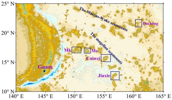
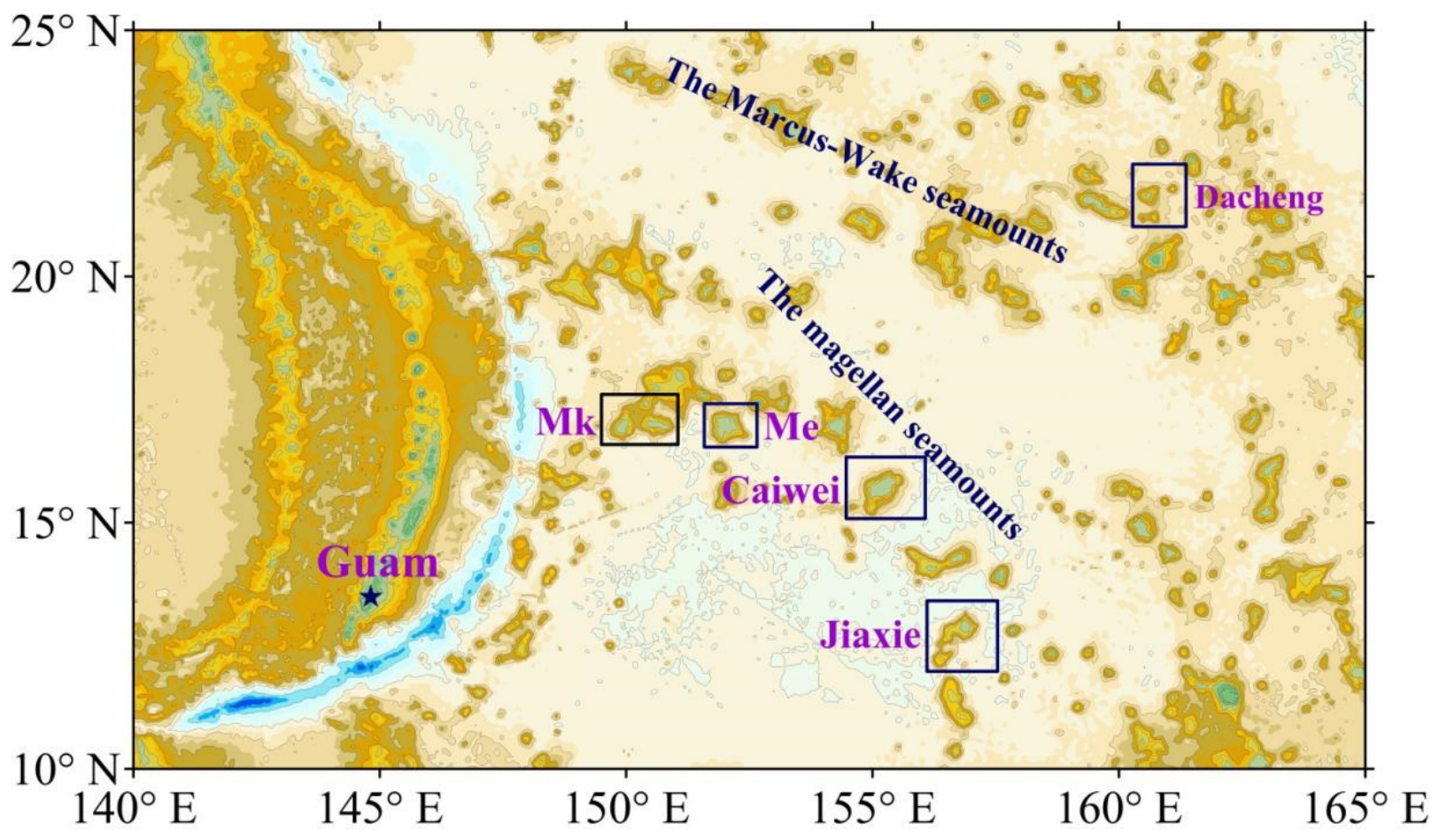
This study covers four seamounts of the Magellan Seamount Chain in the western Pacific, namely MK, ME, Caiwei, and Jiaxie, together with the Dacheng Seamount of the Marcus–Wake Seamount Chain (Figure 1). All five are flat-topped guyots with summits at approximately 1500 m depth. Crusts are deposited on their flank slopes, predominantly within a water depth range of ~1500–3500 m.
Figure 1.
Locations of five seamounts in the Western Pacific.
2.2. Survey Data
Since the mid-1990s, survey cruises organized by the China Ocean Mineral Resources Research and Development Association have carried out geological station sampling and topographic surveying on these five seamounts. Dredging, shallow drilling, and television grab sampling together yielded 288 crust thickness data points, whereas bathymetric surveying was performed with an EM120 deep-water multibeam echo sounder, producing gridded data at a spatial resolution of 100 m × 100 m. Table 1 summarizes the statistical crust thickness parameters of the five seamounts. Because the data points are sparse, variogram modeling based on a single seamount yields unsatisfactory results even for the MK Seamount, which has the largest dataset (77 geological survey stations) [8]. The analysis below therefore combines “multiseamount data integration” with “relative water depth constraints on point-pair searching” to perform multimodel variogram simulation, with the aim of obtaining a greater number of more robust variogram models.
Table 1.
Statistical characteristics of cobalt-rich ferromanganese crust thickness data from the Magellan Seamount Group and the Dacheng Seamount, along with their transformed values.
3. Methodology
3.1. Multiseamount Data Integration
Under the “multiseamount combined data” approach, crust thickness data were transformed for five western Pacific guyots, namely MK, ME, Caiwei, Jiaxie, and Dacheng, all of which share similar geomorphological features and crust thickness distribution characteristics. The transformed combined dataset has a uniform mean (58 mm) and similar standard deviations (32.32 mm). The transformations were carried out as follows:
First, we divided the mean of the data sampled from one seamount (e.g., guyot Mk) by the mean of those collected from another (i.e., guyot Me, Caiwei, Jiaxie, or Dacheng). The resulting quotient, Ti = MeanMk/Meani, i = Mk, Me, Caiwei, Jiaxie, Dacheng, served as the weighting coefficient for transforming the unified data. Letting the unified data be
where Ni is the number of data points for seamount i, the data from the selected seamounts are given by
Zi,j (i = Mk, Me, Caiwei, Jiaxie, Dacheng; j = 1, 2, …, Ni),
Zi,j = Ti × Zi,j (i = Mk, Me, Caiwei, Jiaxie, Dacheng; j = 1, …, Ni)
The statistical parameters of the combined dataset are presented in Table 1.
3.2. Data Preprocessing
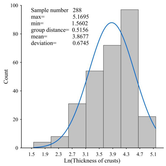
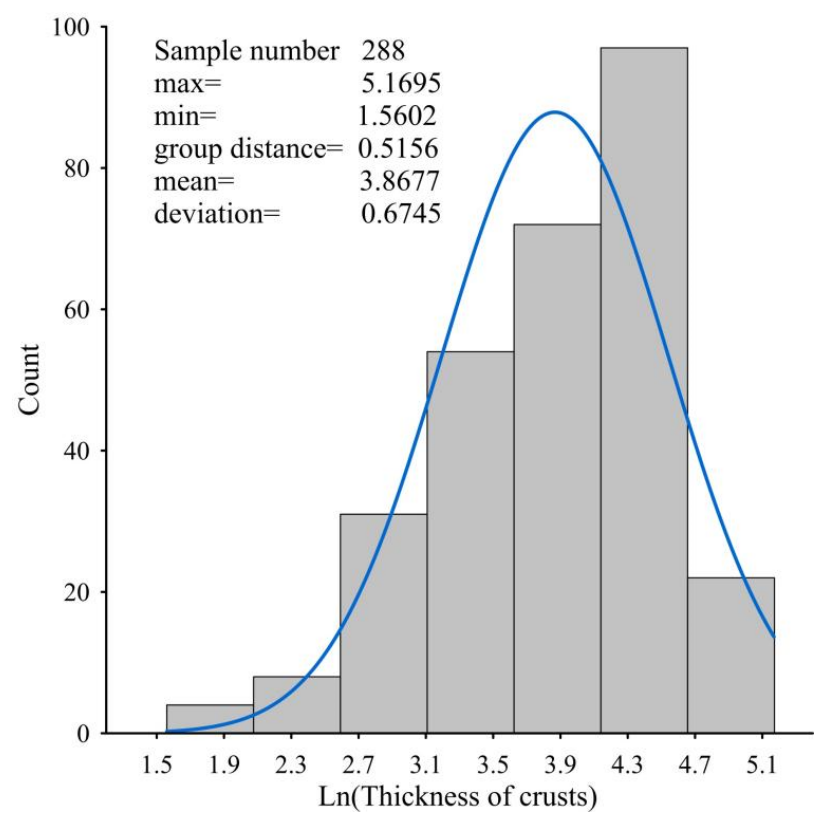
To ensure statistical stationarity, the dataset was tested for conformity to a normal or lognormal distribution, and outliers were removed until one of these was satisfied. Testing confirmed that the combined dataset follows a lognormal distribution; its statistical parameters and distribution characteristics are shown in Figure 2. After logarithmic transformation, the data were therefore treated as weakly stationary random variables for the variogram experiments [31].
Figure 2.
Statistical parameters and normality characteristics of the log-transformed integrated dataset.
The integrated dataset was finally formatted as the Supplementary File WP288.txt, which lists, for each data point, the x-coordinate (longitude; first row), the y-coordinate (latitude; second row), the water depth (positive values; third row), and the natural logarithm of crust thickness (fourth row). Water depth here replaces the vertical coordinate of conventional three-dimensional data.
3.3. Experimental Variogram
3.3.1. Parameter File of the Variogram
The parameter file GAMV.PAR [32] of the variogram program was modified by adding the minimum and maximum water depth limits at the data stations, removing the directional search parameters, and introducing the “number of depth tolerances” (ndp) and the “relative water depth,” defined as the absolute difference in water depth between paired points. For example, ndp = 5 with depth tolerances of 100 m, 200 m, 300 m, 400 m, and 500 m (listed in a single column), or ndp = 1 with a depth tolerance of 200 m (see Supplementary Materials). All other parameters retain the meanings given in the original file [32]. The modified file was renamed GAMV_rd.PAR to distinguish it from the original GAM.PAR.
3.3.2. Variogram Program
The source codes and parameter files, comprising the main program GAMV.for, the header file GAMV.inc, the subroutine CHKNAM.FOR, and the parameter file GAMV.PAR, derive from GSLIB 1998 [32]. To compute the distance–relative water depth variogram, the GAMV source code was modified and applied within the framework of the GSLIB copyright agreement, retaining the original developers’ credits as the copyright terms require. All modifications are annotated in the source code (see Supplementary Materials). To distinguish the modified files from the original code, their names carry the suffix “_rd” (e.g., GAMV_rd.f), the sole exception being the unmodified subroutine CHKNAM.FOR.
3.3.3. Variogram Program Environment and Execution
The variogram program is executed as follows:
(1) Install a Windows Fortran compiler.
(2) Create a working directory, e.g., /gamv_rd.
(3) Copy the files GAMV_rd.f, GAMV_rd.inc, and CHKNAM.FOR into this working directory.
(4) Open the Fortran compiler and create an empty Fortran Console Application Project, setting the project name to, e.g., Gamv.
(5) Add GAMV_rd.f and CHKNAM.FOR to the Source Files, and GAMV_rd.inc to the Header Files.
(6) Copy the parameter file GAMV_rd.PAR and the data file WP288.CSV into the project directory /gamv_rd/Gamv.
(7) Compile and run GAMV_rd.f, and then check the output file Dc.out. If the results are unsatisfactory, adjust the parameters in GAMV_rd.PAR and repeat until they are satisfactory.
(8) Fit the experimental variogram to the theoretical spherical and sinusoidal models.
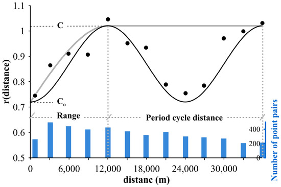
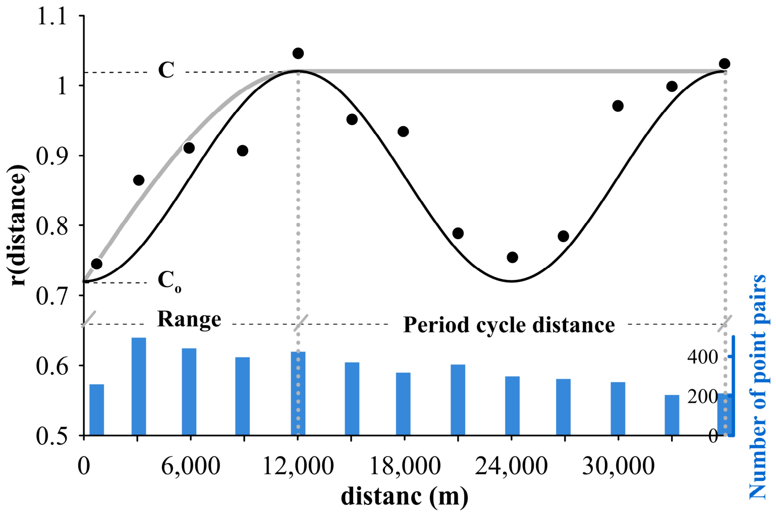
The fitting proceeded in four steps. First, the Dc.out data were used to generate a two-dimensional “distance–semivariance” scatter plot (Figure 3). Second, the nugget (Co), sill (C), range, and period distance (period) were estimated empirically and substituted into Equations (2) and (3) to obtain the mean squared error between theoretical and experimental values. Third, these four parameters were fine-tuned within a limited range, and the mean squared error was recalculated iteratively until it reached a minimum, with a simple Fortran program used to identify the fine-tuned values rapidly. Finally, the optimized parameters were substituted into Equations (2) and (3) to derive the theoretical variogram functions.
Figure 3.
Experimental distance–relative water depth variogram of crust thickness from western Pacific seamounts (black scatter points), computed from 288 integrated crust thickness data points from the Magellan Seamount Group and the Dacheng Seamount (Table 1). The black and gray solid curves are the theoretical curves fitted to the sinusoidal and spherical models, respectively.
3.4. Kriging Interpolation Method
3.4.1. Datasets
This study uses two datasets. The first contains the known survey station data of the study area, formatted as the file WP288.txt (see Supplementary Materials); for the Dacheng Seamount, for example, the file Dacheng20.txt holds the geographic coordinates, water depths, and log-transformed crust thicknesses of 20 stations. The second contains the bathymetric data of the study area, that is, the geographic coordinates and corresponding water depths (positive values), formatted as shown in the Supplementary Materials; the Dacheng Seamount bathymetric dataset is named DCdepth.txt.
3.4.2. Kriging Parameter File
The geostatistical programs used here derive from the GSLIB package developed at Stanford University [32]. Applying the distance–relative water depth spherical or sinusoidal model variogram and computing the Kriging interpolation required modifying KB3D.for, the header file KB2D.inc, and the parameter file KB2D.PAR under the copyright terms and agreements of GSLIB 1998; the introductory remarks in the source code of KB2D_rd.for are reproduced in the Supplementary Materials. The relevant modifications are annotated in the source code (see Supplementary Materials). KB3D_rd.for adds the sinusoidal model, water depth range restrictions, and relative water depth evaluation for information pairs to the original code, and the water depth restrictions, a bathymetric data file such as DCdepth.txt, the sinusoidal wave period, and the sinusoidal model are likewise added to the original contents. All modified programs are submitted as Supplementary Materials. Their file names carry the suffix “_rd” (e.g., KB3D_rd.for) to distinguish them from the original code, the sole exception being the unmodified subroutine CHKNAM.FOR.
3.4.3. Kriging Program
The source codes and parameter files of the Kriging program, comprising the main program KB3D.for, the header file KB2D.inc, the subroutine CHKNAM.FOR, and the parameter file KB2D.PAR, were all sourced from GSLIB 1998 [32]. To apply the distance–relative water depth variogram, the source code was modified within the framework of the GSLIB copyright agreement, and all modifications are annotated in the source code (see Supplementary Materials). Every file name except that of the unmodified subroutine CHKNAM.FOR carries the suffix “_rd” (e.g., KB3D_rd.for) to distinguish it from the original code. Relative to the original KB3D.for, KB3D_rd.for incorporates the sinusoidal model, water depth range restrictions, and relative water depth evaluation for information pairs, while KB2D_rd.PAR retains the contents of the original file and adds the water depth restrictions, a bathymetric data file, and sinusoidal model parameters such as the wave period. All modified program files are provided in the Supplementary Materials.
3.4.4. Kriging Program Environment and Execution
The Kriging program is executed as follows:
- (1)
- Install a Windows Fortran compiler.
- (2)
- Create a working directory, e.g., D:/Krig_rd.
- (3)
- Copy the files KB3D_rd.for, KB2D_rd.inc, and CHKNAM.FOR into this working directory.
- (4)
- Open the Fortran compiler, create an empty Fortran Console Application Project, and set the project name to, e.g., “Kriging.”
- (5)
- Add KB3D_rd.for and CHKNAM.FOR to the Source Files, and KB2D_rd.inc to the Header Files.
- (6)
- Copy the parameter file KB2D_rd.PAR and the data file Dacheng20.CSV into the project directory D:/Krig_rd/Kriging.
- (7)
- Compile and run KB3D_rd.for, and then open the output file Dacout.txt to inspect the results. If the results are unsatisfactory, adjust the parameters in KB2D_rd.PAR and repeat until they are satisfactory.
4. Results and Discussion
4.1. Experimental and Theoretical Distance–Relative Depth Variograms
Following the procedure in Section 3.3, the experimental variogram values were computed and plotted against distance as a two-dimensional scatter plot (Figure 3). Fitting the scatter points to the spherical and sinusoidal models yielded the variograms given by Equations (2) and (3), respectively:
where a denotes the range of the spherical model, period the distance of one period in the sinusoidal model, C and C0 the sill and nugget, respectively, and dis the point-pair distance. The fitted curves of both models are shown in Figure 3.
Point pairs were searched at a relative water depth interval of 200 m, at which the spatial autocorrelation of crust thickness is expressed most effectively with distance as the variable, giving a uniform distribution of point pairs within each lag group and a sufficient number of pairs overall. The blue bars in Figure 3 show the number of point pairs found in each lag group, all of which exceed 200.
The spherical model variogram in Figure 3 closely resembles the distance–relative water depth variogram of the Magellan Seamounts [8]: their ranges are comparable, their sills identical (1.02), and their nuggets differ by only 0.3. The striking similarity among spherical model variograms simulated jointly from different combinations of western Pacific seamounts suggests that such variograms can describe the spatial autocorrelation of crust thickness across a broad range of western Pacific seamounts, which is a prerequisite for applying the variogram to other areas.
Based on the experimental variogram results, the parameters were set to period = 24,000 m, c0 = 0.70, c = 1.00, and a = 12,000 m. Substituting these values into Equations (2) and (3) yields the spherical and sinusoidal model variograms, respectively.
The spatial autocorrelation of crust thickness expressed by the sinusoidal model variogram varies with a clear periodicity, implying that a common mechanism governs crust thickness distribution on seamount flanks. As the volcanoes became gradually extinct after the Late Cretaceous, the seamounts cooled, contracted, and subsided while being eroded by the circum-seamount current and disturbed by seismic activity [33,34,35,36]. The flank slopes, built up by successive layered volcanic eruptions, became vulnerable to failure in their middle portions once their width exceeded a certain scale (e.g., 24,000 m). Each failure removed the in situ sediments and allowed crust deposition to recommence, thereby altering the spatial pattern of crust thickness [29]. The observed periodicity therefore reflects a cyclic alternation between continuous crust deposition and its resetting and renewal.
Expressed by this function, the spatial autocorrelation of crust thickness is enhanced at distances beyond the range, which permits a larger information-point search radius during Kriging interpolation. More information points can consequently be incorporated into the Kriging equations, benefiting the spatial interpolation of crust thickness in study areas with sparse stations.
4.2. Comparison of the Multiseamount “Distance–Relative Water Depth” Variogram with Traditional Methods
- (1)
- Multiseamount combined data versus single-seamount data
The blue histogram in Figure 3 shows that each search group contains 200 to 500 point pairs. By comparison, Figure 8 of reference [8], which presents the distribution of search point pairs derived from the 77 data points of the MK Seamount, one of the better-sampled seamounts, shows only 11 to 64 pairs per search group, a clearly inadequate statistical sample that carries insufficient information. The multiseamount combined data, in contrast, supply enough search point pairs to make the resulting variogram statistically far more convincing.
- (2)
- Comparison between the “distance–relative water depth” and “distance–direction” variograms
Figure 4 of reference [8] and Figure 3 of reference [7] present “distance–direction variograms” in which the two-dimensional scatter plots of experimental variogram values oscillate randomly about the mean squared error in every direction, revealing no spatial autocorrelation. Figure 3 of the present study, by contrast, clearly exhibits autocorrelation when distance is taken as the variable.
The reason for this lies in the search constraint applied before the mean semivariance of the point pairs is calculated. Once the relative water depth, that is, the water depth difference between paired points, is fixed, the mean semivariance depends on distance alone and thus approximates a one-dimensional spatial function. This behavior is one of the mathematical characteristics of the spatial distribution of seamount crust resources. Differences in water depth also produce differences in ferromanganese crust mineralization, so crust thickness shows stronger spatial autocorrelation within a restricted depth range. Water depth therefore acts here as a mineralization-controlling factor rather than as a spatial position parameter. Because crusts occur only at the seamount surface and are less than 30 cm thick, their spatial distribution resembles that of a three-dimensional surface [7] rather than a three-dimensional volumetric variable.
4.3. Kriging Spatial Interpolation of the Dacheng Seamount
The sinusoidal model variogram (Equation (3)) was first coded in Fortran (see Section 3.3.3). The parameter file KB2D_rd.PAR was then configured with an interpolation grid spacing of 2000 m × 2000 m, a search radius of 36,000 m, a sinusoidal wavelength (period) of 24,000 m, and a relative water depth tolerance of 200 m. The grid spacing was kept as small as possible while still ensuring that every grid cell contained enough interpolation information points, and the final value was selected after repeated trial calculations. The nugget C0, sill C, and range a were set to 0.72, 1.02, and 12,000 m, respectively. All these parameters are specified in KB2D_rd.PAR. Finally, KB3D_rd.for was compiled and run in the Fortran compiler following the procedure in Section 3.4.4, and the resulting interpolated crust thicknesses for the Dacheng Seamount were written to the output file Dacout.txt (see Supplementary Materials).
To partially correct the systematic bias introduced by the logarithmic transformation [37,38], the following exponential back-transformation was adopted:
where
is the estimate back-transformed to the original data space,
is the Kriging estimate in log-space,
is the Kriging variance in log-space.
On the Dacheng Seamount (T5 = 0.9547; Table 1), the values in 148 grid cells (j = 1, …, 148), each with an area of 4 km2, were estimated. Using (4), estimates that more closely approximate the conditional mean of the original data were obtained.
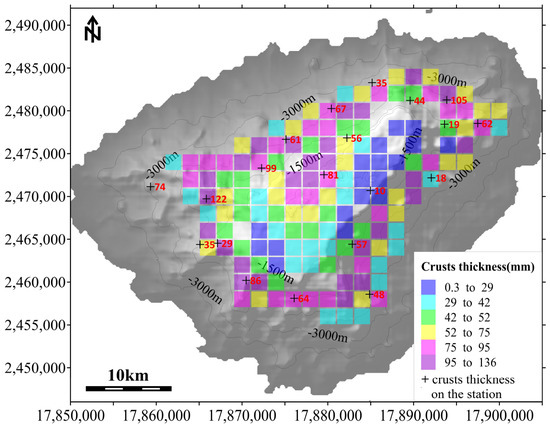
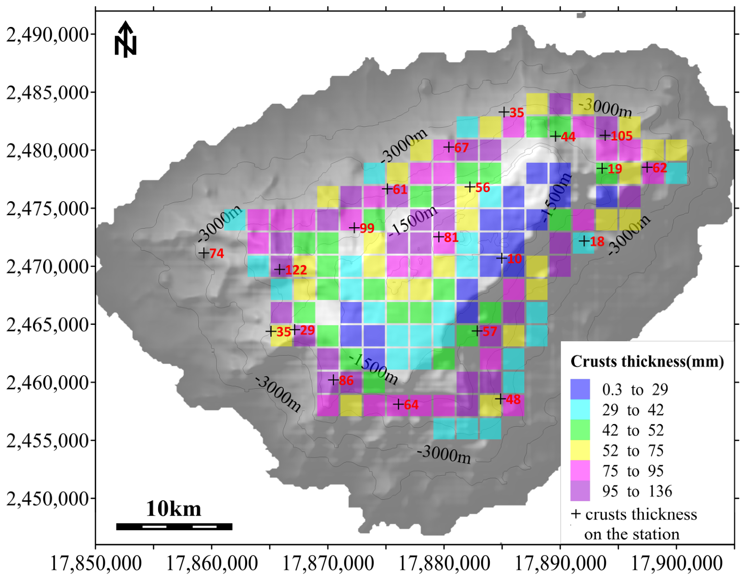
Table 2 lists the statistical parameters of the 20 survey station data points from the Dacheng Seamount alongside those of the 148 grid node interpolation points (2000 m × 2000 m). The interpolated values have a mean of 59.9 mm and a mean deviation of 24.3 mm, both slightly larger than the corresponding values of 58.6 mm and 23.5 mm for the original station data. This small discrepancy arises from the optimal unbiased Kriging algorithm and may also reflect statistical errors introduced by the lognormal transformation and its back-transformation. To remove the bias, each estimate (Ti) was multiplied by a correction coefficient of 58.6/59.9 = 0.978, giving a corrected mean of 58.6 mm and a corrected mean deviation of 23.8 mm, both very close to the original data. The corrected estimates Thj constitute the final results. These values for the 148 grid cells were classified into five crust thickness grades, assigned distinct colors, and overlaid on the seamount topographic map to produce Figure 4.
Table 2.
Statistical parameters of crust thickness data from geological sampling stations and Kriging estimates for the Dacheng Seamount.
Figure 4.
Distribution of ferromanganese crust thickness on the Dacheng guyot estimated by Kriging interpolation.
4.4. Analysis of the Spatial Interpolation Effects
Previous studies have estimated crust thickness in unsampled areas either by averaging the known thicknesses or by applying spatial interpolation methods such as inverse distance weighting (IDW). Here, four methods were applied separately to estimate values at the known stations, namely Kriging based on the sine model variogram (sine Kriging), Kriging based on the spherical model variogram (spherical Kriging), IDW, and the regional mean method, and their mean relative errors were compared to assess interpolation performance.
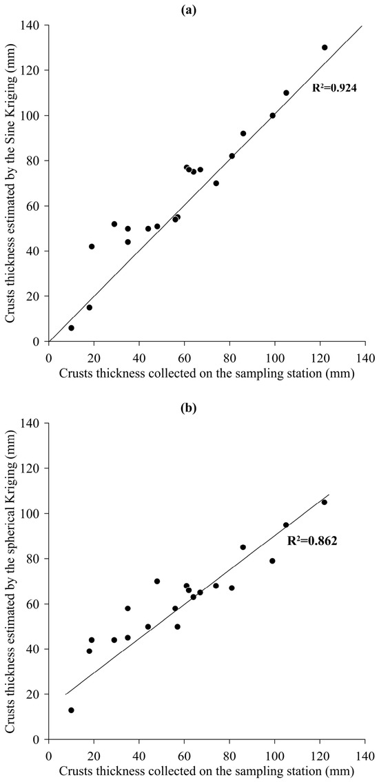
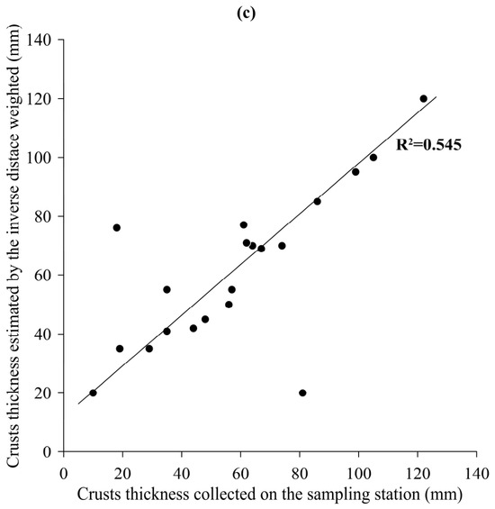
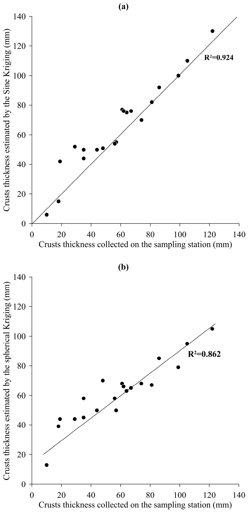
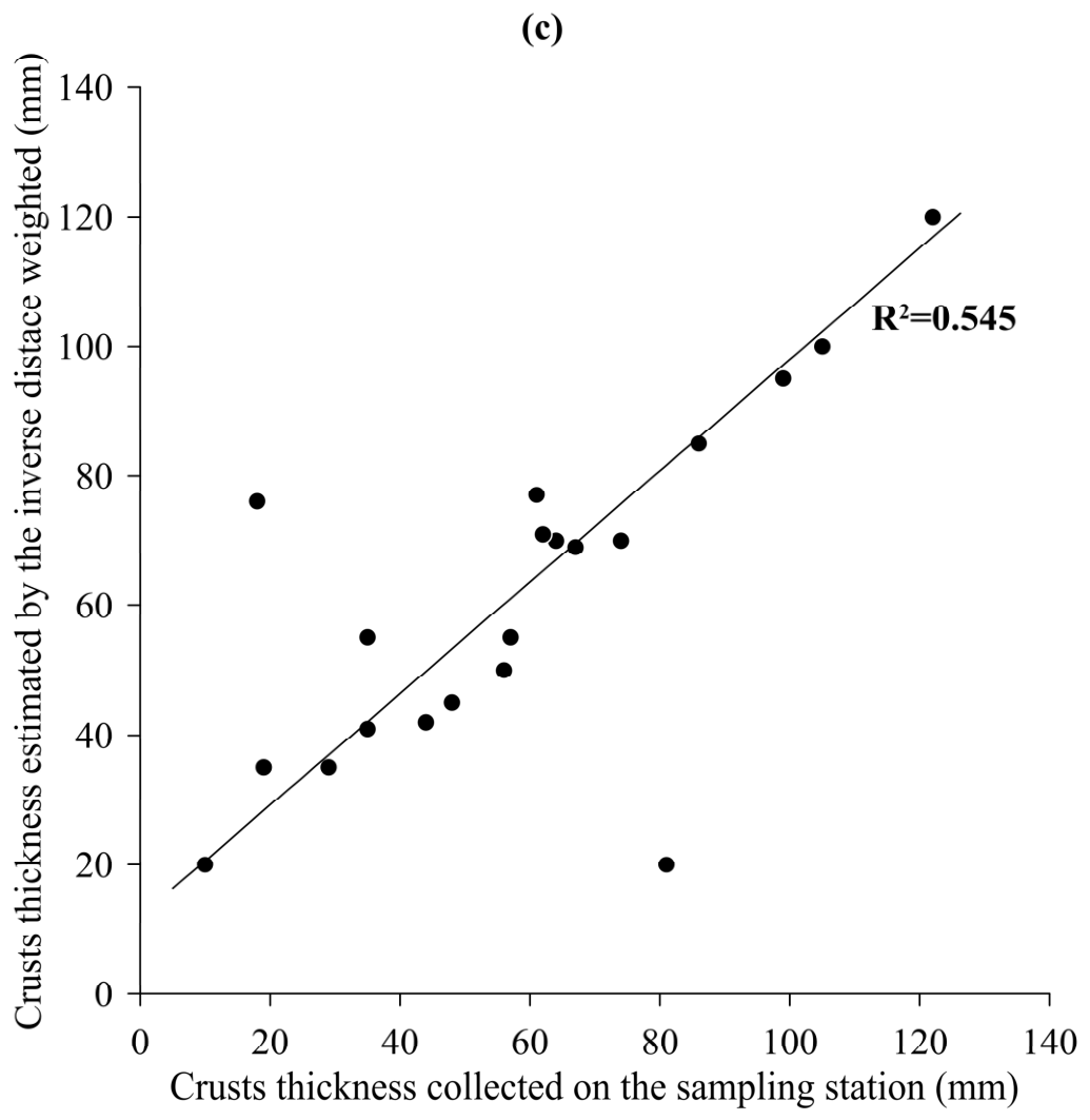
Figure 5 plots the surveyed crust thickness data from the 20 stations against the corresponding estimates. In Figure 5a, the sine Kriging estimates lie along the y = x line, indicating a close fit to the known station data, with a coefficient of determination (R2) of 0.924 and a mean relative error of 14.08%. As shown in Figure 5b, the spherical Kriging estimates deviated to some extent from the y = x line but remained well correlated with the original data, with an R2 value of 0.862 and a mean relative error of 18.43%. As shown in Figure 5c, the IDW estimates deviated further from the y = x line, showing an R2 value of 0.545 and a mean relative error of 20.40%. Taking the mean of the 20 stations as the estimate for every station gives a relative error of 40.10%.
Figure 5.
Known and estimated ferromanganese crust thicknesses at the 20 survey locations on the Dacheng guyot. The vertical coordinate is crust thickness, estimated by (a) sine model Kriging, (b) spherical model Kriging, and (c) inverse distance weighting.
Comparing the four methods shows that sine Kriging and spherical Kriging achieve the highest correlation coefficients between estimated and known station values and the smallest mean relative errors, with the former outperforming the latter. Both clearly surpass IDW and are far superior to the regional mean method.
The slope area of the Dacheng Seamount (water depth range 1500–3500 m) has an area of approximately 600 km2.
The slope of the Dacheng Seamount, which spans a water depth range of 1500–3500 m and covers approximately 600 km2, hosts only 20 survey stations, a density of one station per 50 km2. Describing the spatial distribution of crust thickness accurately from such sparse information points is difficult. Accuracy would improve most effectively with a higher station density, but the prohibitive cost of surveys makes this infeasible. Under these constraints, Kriging interpolation that exploits the spatial autocorrelation captured by the seamount crust thickness variogram offers an affordable alternative.
These results provide preliminary evidence that Kriging with the sine and spherical model “distance–relative water depth” variograms fitted from multiseamount combined data is an effective interpolation tool, and they further confirm that a variogram fitted under relative water depth constraints performs acceptably. The present work and earlier studies [8,9], although based on different seamount datasets, have produced similar “distance–relative water depth” variograms, indicating that variograms fitted from multiseamount combined data possess a degree of statistical robustness. Such variograms may therefore be suitable for spatial interpolation on other, comparable seamounts.
Compared with traditional mineral deposits, seamount crusts exhibit unique characteristics. (1) They are distributed on the surface of seamounts, with thicknesses ranging approximately from 1 to 300 mm. They represent three-dimensional surface data rather than true three-dimensional data [7,8]; therefore, water depth cannot be considered as a third spatial dimension, as discussed in our previous work. (2) Their thickness autocorrelation is isotropic. From this perspective, the variogram is a function of the distance as the sole variable. Although this function has only one variable (constrained by relative water depth), it can reflect the spatial autocorrelation of two-dimensional crust thickness data.
5. Conclusions
The “distance–relative water depth” experimental variogram was calculated by combining crust thickness data from five seamounts of the Magellan and Marcus–Wake seamount chains. Within the range, the experimental variogram data conform to the traditional spherical model; over the larger distance space that encompasses the range, they display a marked periodicity consistent with the sine model. Two variograms were fitted on the basis of these features:
(1) The spherical model variogram of crust thickness for the five seamounts. This function closely resembles the variogram derived from four seamounts, indicating that it possesses a degree of robustness, or representativeness, across the western Pacific seamount region.
(2) The sine model variogram of seamount crust thickness. Its periodicity implies that common structural features on seamount flanks constrain the distribution of crust thickness. Once the flank distance exceeds 12,000 m, for example, collapse becomes more likely, clearing sediments from the slope surface and re-initiating ferromanganese crust deposition, which in turn alters the spatial distribution of crust thickness.
The water depth constraint for point-pair searching was set at 200 m when the experimental variogram was calculated. Variogram autocorrelation is most pronounced when the absolute water depth difference between paired points does not exceed this value. Within the range, semivariance decreases as distance decreases, and semivariance varies with distance in a clearly regular manner that is readily fitted by known functions. In essence, the relative water depth constraint reflects the fact that crust thickness is more strongly autocorrelated along the isobath direction.
For interpolation with the spherical model variogram, the optimal search radius for information points equals the range, that is, 12,000 m, whereas with the sine model variogram the radius can be extended to 24,000 m or 36,000 m. The sine model variogram thus permits a larger search radius, a considerable advantage for spatial interpolation in study areas with extremely sparse geological stations such as the Dacheng Seamount. Kriging with the two variograms gave mean relative errors of 14.08% and 18.43% for the 20 stations, lower than the 20.40% obtained by IDW and far superior to the 40.10% of the regional mean method.
The variogram models derived from the five-seamount combined data apply to western Pacific seamounts of similar geomorphology, such as those with flat-topped morphology and comparable water depth ranges. Seamounts with different morphological features or geological settings, including conical seamounts, ridges, and other deep-sea regions, require validation before the models can be applied to them. Future work will expand the number of sample seamounts to obtain more broadly applicable variogram models and thereby advance deep-sea ferromanganese crust resource assessment.
Although the variogram derived from multiseamount combined data under water depth constraints has performed well in application, further investigation remains necessary. The spatial characteristics of the flank topography and geomorphology that control crust distribution, together with their geological history, must be studied to assign clear geological significance to the periodicity of the sine model variogram. Crust thickness data from additional seamounts must also be analyzed to verify the robustness and general applicability of variograms simulated from multiseamount combined data and to exclude the possibility that the sine model merely reflects overfitting.
The significance of this paper and our previous work lies in introducing a new variogram to fit the spatial autocorrelation of seamount crust thickness data and perform geostatistical interpolation of these data. To date, few studies related to the geostatistical interpolation of seamount crust thickness data have been reported. One of the reasons for this is that traditional variograms fail to capture the spatial autocorrelation of crust thickness data. This paper, together with our previous work [7,8], introduces a variogram with distance (controlled by the relative water depth) as the variable in an attempt to apply geostatistical methods in the field of seamount resource evaluation.
Supplementary Materials
The following supporting information can be downloaded at: https://www.mdpi.com/article/10.3390/min16100982/s1, WP288.txt (The integrated dataset from five seamounts). GAMV_rd.f (The main program file of the variogram modified according to GAMV.par). CHKNAN.for (A subroutine file of the main program). GAMV_rd.inc (Header file of main program modified according to GAMV.inc). GAMV_RD.par (Parameter file of the variogram program modified according to GAMV.par). Dacheng20.txt (Survey station data of Dacheng seamount formatted as the file WP288.txt). DCdepth.txt (The Dacheng Seamount bathymetric dataset). KB2D_rd.inc (Header file of main program modified according to KB2D.INC). KB2D_rd.par (The parameter file of the Kriging program modified according to KB2D.par). KB3D_rd.for (The program file of the Kriging modified according to KB3D.for) [32].
Author Contributions
D.D. conceived the paper. D.D. and S.Y. are co-first authors. S.Y. and X.R. jointly wrote the main manuscript. The other authors contributed to data acquisition, data analysis, and figure preparation. All authors reviewed and revised the manuscript. All authors have read and agreed to the published version of the manuscript.
Funding
This research was funded by the National Key Research and Development Program, grant number 2025YFF0517000 and the National Natural Science Foundation of China, grant number 42276080.
Data Availability Statement
Data are available on request from the authors. The data are not publicly available due to [data publication agreement of COMRA].
Acknowledgments
The data were provided by projects sponsored by the Ministry of Natural Resources (MNR) of China and China Ocean Mineral Resources Research and Development Association (COMRA). The authors thank all scientists of the surveying cruises.
Conflicts of Interest
The authors declare no conflict of interest.
References
- Staudigel, H.; Koppers, A.P.; Lavelle, J.W.; Pitcher, T.J.; Shank, T.M. Defining the word “seamount”. Oceanography 2010, 23, 20–21. [Google Scholar] [CrossRef] [Scilit]
- Hein, J.R. Cobalt-rich ferromanganese crusts: Global distribution, composition, origin and research activities. In Proceedings of the International Seabed Authority Workshop Minerals Other Than Polymetallic Nodules of the International Seabed Area, Kingston, Jamaica, 26–30 June 2000; pp. 26–30. [Google Scholar]
- Hein, J.R.; Koschinsky, A.; Bau, M.; Manheim, F.T.; Kang, J.K.; Roberts, L. Cobalt-rich ferromanganese crusts in the Pacific. In Handbook of Marine Mineral Deposits; Cronan, D.S., Ed.; CRC Press: London, UK, 1999; pp. 239–279. [Google Scholar] [CrossRef] [Scilit]
- Verlaan, P.A.; Cronan, D.S.; Morgan, C.L. A comparative analysis of compositional variations in and between marine ferromanganese nodules and crusts in the South Pacific and their environmental controls. Prog. Oceanogr. 2004, 63, 125–158. [Google Scholar] [CrossRef] [Scilit]
- Usui, A.; Okamoto, N. Geophysical and geological exploration of cobalt-rich ferromanganese crusts: An attempt of small-scale mapping on a micronesian seamount. Mar. Georesources Geotechnol. 2010, 28, 192–206. [Google Scholar] [CrossRef] [Scilit]
- Du, D.; Ren, X.; Yan, S.; Shi, X.; Liu, Y.; He, G. An integrated method for the quantitative evaluation of mineral resources of cobalt-rich crusts on seamounts. Ore Geol. Rev. 2017, 84, 174–184. [Google Scholar] [CrossRef] [Scilit]
- Du, D.; Wang, C.; Du, X.; Yan, S.; Ren, X.; Shi, X.; Hein, J.R. Distance-gradient-based variogram and Kriging to evaluate cobalt-rich crust deposits on seamounts. Ore Geol. Rev. 2017, 84, 218–227. [Google Scholar] [CrossRef] [Scilit]
- Du, D.; Yan, S.; Yang, F.; Zhu, Z.; Song, Q.; Yang, G. Kriging interpolation for evaluating the mineral resources of cobalt-rich crusts on Magellan Seamounts. Minerals 2018, 8, 374. [Google Scholar] [CrossRef] [Scilit]
- Hein, J.R.; Conrad, T.A.; Dunham, R.E. Seamount characteristics and mine-site model applied to exploration-and mining-lease-block selection for cobalt-rich ferromanganese crusts. Mar. Georesources Geotechnol. 2009, 27, 160–176. [Google Scholar] [CrossRef] [Scilit]
- Yan, S.; Shi, X.; Yang, G.; Du, D.; Liu, Y.; Ye, J.; Ren, X.; Zhu, Z.; Hao, Y. Method for assessing the thickness of cobalt-rich crust on seamounts and its application on the Il’ichev Guyot. Minerals 2022, 12, 1538. [Google Scholar] [CrossRef] [Scilit]
- Usui, A.; Someya, M. Distribution and composition of marine hydrogenetic and hydrothermal manganese deposits in the northwest Pacific. Geol. Soc. Lond. Spec. Publ. 1997, 119, 177–198. [Google Scholar] [CrossRef] [Scilit]
- Zhang, F.Y.; Zhang, W.; Zhu, K.; Zhang, H.; Xiaoyu, Z. Distribution characteristics of cobalt-rich ferromanganese crust resources on submarine seamounts in the western Pacific. Acta Geol. Sin. 2008, 82, 796–803. [Google Scholar] [CrossRef] [Scilit]
- David, M. (Ed.) Geostatistical ore reserve estimation. In Developments in Geomathematics; Elsevier: Amsterdam, The Netherlands, 1977; p. 364. [Google Scholar]
- Journel, A.G.; Huijbregts, C.J. Mining Geostatistics; Academic Press Inc.: London, UK, 1978. [Google Scholar]
- Journel, A.G. Geostatistics for the Environmental Sciences: An Introduction; US Environmental Protection Agency, Environmental Monitoring Systems Laboratory: Washington, DC, USA, 1987. [Google Scholar]
- Journel, A.G. New Distance Measures: The route toward truly nongaussian geostatistics. Math. Geol. 1988, 20, 459–475. [Google Scholar] [CrossRef] [Scilit]
- Journel, A.G. Fundamentals of Geostatistics in Five Lessons; American Geophysical Union: Washington, DC, USA, 1989; Volume 8, pp. 2–8. [Google Scholar]
- Cressie, N.A. Statistics for Spatial Data; Wiley: New York, NY, USA, 1993. [Google Scholar]
- Cressie, N.; Hawkins, D.M. Robust estimation of the variogram: I. J. Int. Assoc. Math. Geol. 1980, 12, 115–125. [Google Scholar] [CrossRef] [Scilit]
- Omre, H. The variogram and its estimation. In Geostatistics for Natural Resources Characterization; Springer: Dordrecht, The Netherlands, 1984; pp. 107–125. [Google Scholar]
- Armstrong, M. Improving the estimation modelling of the variogram. In Geostatistics for Natural Resources Characterization; Verly, G., David, M., Journel, A.G., Marechal, A., Eds.; Springer: Dordrecht, The Netherlands, 1984; pp. 1–19. [Google Scholar]
- Isaaks, E.H.; Srivastava, R.M. Spatial continuity measures for probabilistic and deterministic geostatistics. Math. Geol. 1988, 20, 313–341. [Google Scholar] [CrossRef] [Scilit]
- Isaaks, E.H.; Srivastava, R.M. An Introduction to Applied Geostatistics; Oxford University Press: New York, NY, USA, 1989. [Google Scholar]
- Chu, F.Y.; Sun, G.S.; Li, X.M.; Ma, W.L.; Zhao, H.Q. The growth habit Controlling factors of the cobalt-rich crusts in seamount of the central Pacific. J. Jilin Univ. (Earth Sci. Ed.) 2005, 35, 320–325. [Google Scholar]
- Hein, J.; Conrad, T.; Staudigel, H. Seamount mineral deposits: A source of rare metals for high-technology industries. Oceanography 2010, 23, 184–189. [Google Scholar] [CrossRef] [Scilit]
- Ma, W.L.; Yang, K.H.; Bao, G.S.; Zhang, K.; Dong, R.Z.; Chu, F.Y. Spatial distribution study of cobalt rich crusts ore formation on the central Pacific seamount. Acta Oceanol. Sin. 2014, 36, 77–89. (In Chinese) [Google Scholar]
- Cheng, Y.; Jiang, X.; Song, S.; Sun, S.; Yu, J. Delineation of cobalt crust block estimation of cobalt crust resource of Govorov Guyot Magellan seamounts Pacific Ocean. J. Jilin Univ. (Earth Sci. Ed.) 2015, 45, 1642–1656. [Google Scholar]
- Yeo, I.A.; Howarth, S.A.; Spearman, J.; Cooper, A.; Crossouard, N.; Taylor, J.; Turnbull, M.; Murton, B.J. Distribution of and hydrographic controls on ferromanganese crusts: Tropic Seamount, Atlantic. Ore Geol. Rev. 2019, 114, 103131. [Google Scholar] [CrossRef] [Scilit]
- Du, D.; Yan, S.; Yang, G.; Shi, F.; Zhu, Z.; Song, Q.; Yang, F.; Cui, Y.; Shi, X. Depositional patterns constrained by slope topography changes on seamounts. Sci. Rep. 2020, 10, 20534. [Google Scholar] [CrossRef] [Scilit] [PubMed]
- Hino, H.; Usui, A. Regional and fine-scale variability in composition and structure of hydrogenetic ferromanganese crusts: Geological characterization of 25 drill cores from the Marcus-Wake seamounts. Mar. Georesources Geotechnol. 2022, 40, 415–437. [Google Scholar] [CrossRef] [Scilit]
- Matheron, G. La Théorie des Variables Régionalisées et ses Applications; Ecole Nationale Superieure des Mines: Paris, France, 1971. [Google Scholar]
- Deutsch, C.V.; Journel, A.G. GSLIB Geostatistical software Library and User’s Guide, 2nd ed.; Oxford University Press: New York, NY, USA, 1998. [Google Scholar]
- Suominen, V. Late Precambrian plastic deformation in crystalline limestone in Kumlinge, south-west Finland. Bull. Geol. Soc. Finl. 1973, 45, 49–52. [Google Scholar] [CrossRef] [Scilit]
- Speckbacher, R.; Behrmann, J.H.; Nagel, T.J.; Stipp, M.; Devey, C.W. Splitting a continent: Insights from submarine high-resolution mapping of the Moresby Seamount detachment, offshore Papua New Guinea. Geology 2011, 39, 651–654. [Google Scholar] [CrossRef] [Scilit]
- Ebert, A.; Herwegh, M.; Berger, A.; Pffner, A. Grain coarsening maps for polymineralic carbonate mylonites: A calibration based on data from different Helvetic nappes (Switzerland). Tectonophysics 2008, 457, 128–142. [Google Scholar] [CrossRef] [Scilit]
- Staudigel, H.; Schmincke, H.U. The Pliocene seamount series of La Palma/Canary Islands. J. Geophys. Res. 1984, 89, 11195–11215. [Google Scholar] [CrossRef] [Scilit]
- Dowd, P.A. Lognormal kriging—The general case. J. Int. Assoc. Math. Geol. 1982, 14, 475–499. [Google Scholar] [CrossRef] [Scilit]
- Rivoirard, J. A review of lognormal estimators for in situ reserves. Math. Geol. 1990, 22, 213–221. [Google Scholar] [CrossRef] [Scilit]

Disclaimer/Publisher’s Note: The statements, opinions and data contained in all publications are solely those of the individual author(s) and contributor(s) and not of MDPI and/or the editor(s). MDPI and/or the editor(s) disclaim responsibility for any injury to people or property resulting from any ideas, methods, instructions or products referred to in the content. |
© 2026 by the authors. Licensee MDPI, Basel, Switzerland. This article is an open access article distributed under the terms and conditions of the Creative Commons Attribution (CC BY) license.