Direct Petrophysical Property Prediction Through Joint Stochastic Inversion of PP and PS Waves

Abstract

Pre-stack seismic inversion provides an effective approach for estimating reservoir properties from seismic observations. However, the use of PP-wave data alone often suffers from insufficient sensitivity to shear-related information, leading to considerable uncertainty in the estimation of multiple coupled reservoir parameters. To alleviate this limitation, this study proposes a PP–PS wave joint stochastic inversion framework for direct prediction of reservoir properties. A statistical rock physics relationship is established to characterize the nonlinear relationship between seismic elastic responses and key reservoir parameters, including porosity, mineral composition, and water saturation. Based on this relationship, a physical-parameter-based PS-wave reflection coefficient approximation is derived and incorporated into the multi-wave inversion formulation. The proposed framework integrates PP- and PS-wave responses within the inversion scheme, enabling simultaneous estimation of multiple petrophysical parameters while accounting for model uncertainty. Synthetic experiments using representative reservoir models demonstrate that introducing PS-wave information improves parameter discrimination and reduces inversion uncertainty compared with conventional PP-wave-only inversion. Application to pre-stack seismic data from China further confirms the capability of the proposed method for characterizing spatial variations in reservoir properties.

1. Introduction

Quantitative characterization of complex reservoirs has become increasingly important as exploration extends deeper and more heterogeneous geological settings. Deep-water and offshore targets, as well as unconventional reservoirs such as carbonates, shales, and natural gas hydrates, commonly exhibit pronounced heterogeneity and strong coupling among reservoir parameters [1,2,3]. Under these conditions, conventional interpretation based primarily on P-wave seismic observations may provide insufficient constraints for reliable estimation of the physical properties required for reservoir characterization.

Pre-stack AVO inversion can be performed using either a single seismic wave mode or multiple wave modes. Single-mode inversion extracts reservoir information from one seismic response, whereas multi-wave inversion combines the complementary sensitivities of different wave types, including PP, P-SV, SV-SV, and SH-SH waves. When only PP-wave data are used, the limited sensitivity of the seismic response to shear-related properties can result in strong parameter trade-offs, particularly for simultaneous estimation of S-wave velocity and density. The inclusion of PS-wave information provides additional sensitivity to shear-wave-related variations and therefore offers complementary constraints on the inversion model. Recent advances in multicomponent seismic acquisition and processing have promoted the use of joint AVO inversion to improve the reliability of lithology and hydrocarbon prediction [4,5]. Bouchaala et al. (2021) estimated P- and S-wave attenuation from three-component walkway VSP and sonic data in an offshore Abu Dhabi oilfield, highlighting the sensitivity of attenuation to fluid content and its potential for carbonate reservoir characterization [6].

Early studies demonstrated the feasibility of extracting elastic information from PP- and PS-wave observations through joint inversion. Stewart [7] investigated the simultaneous estimation of subsurface elastic parameters from PP and P-SV data, while Larsen [8] extended this concept to the joint estimation of P- and S-wave impedances and demonstrated its applicability to field data [9]. Subsequent research has explored different strategies for improving the conditioning and accuracy of the joint inversion problem. For example, velocity-ratio updating has been introduced to improve the prediction of elastic parameters [10], while Bayesian formulations have incorporated covariance information to account for parameter correlations [11]. For layered or unconventional reservoirs, propagator-matrix-based forward modeling provides an alternative means of describing multicomponent seismic responses [12,13]. The exact Zoeppritz formulation has been used to constrain P-wave velocity, S-wave velocity, and density [14], and its combination with first-order approximations and least-squares optimization has enabled direct updating of these elastic parameters [15]. Other studies have developed approximate reflection coefficient formulations for joint inversion, providing computationally efficient alternatives for estimating additional elastic properties [16,17].

Pure S-wave measurements provide another source of information for resolving shear-related reservoir properties. Ray-based elastic impedance derived from pure S-wave data has been investigated for identifying tight gas-bearing sandstone reservoirs [18]. For SV-SV reflections, studies have shown that S-wave velocity and density can be estimated from angle-dependent reflection responses [19]. Related inversion schemes have subsequently been developed using modified SV-SV and SH-SH reflection coefficient approximations, allowing the simultaneous estimation of S-wave velocity and density [20,21,22]. S-wave information can also be obtained from sonic waveforms as a complementary borehole-scale alternative to surface P–SV reflection measurements, while the attenuation analysis of Bouchaala et al. (2016) illustrates the use of sonic waveform data for carbonate reservoir characterization [23]. These investigations demonstrate that shear-wave information can help resolve ambiguities inherent in conventional PP-wave inversion.

The complementary behavior of PP and S-wave responses has also motivated the joint analysis of different wave modes. AVO analysis provides a theoretical basis for comparing the information carried by P- and S-wave reflections. After appropriate simplification of the P-SV and SH reflection coefficients, seismic attributes can be expressed in a form suitable for joint analysis [24]. Sensitivity studies further indicate that combining PP with PS or SS information can improve the identification of gas saturation by exploiting their different responses to elastic and fluid-related variations [25]. In addition, SV-P data recorded using a P-wave source have been investigated as an alternative to conventional P-SV observations, and their joint use with PP data has shown potential for improving reservoir characterization and signal-to-noise performance [26]. Joint interpretation of PP and SS data has also been applied to carbonate reservoirs using nine-component seismic observations [27]. More recently, joint consideration of PP, PS, and SS waves has been explored in the native time domain, providing an initial framework for three-wave seismic reservoir characterization [28].

Despite these developments, most existing multicomponent inversion studies have concentrated on the estimation of elastic parameters or fluid-related indicators, whereas direct prediction of reservoir physical properties from jointly inverted PP and PS data remains relatively limited. In particular, the coupled influence of porosity, mineral composition, and fluid saturation makes it difficult to establish a stable relationship between seismic responses and multiple petrophysical parameters using a single wave mode. This motivates the development of an inversion strategy that can exploit the complementary information of PP and PS waves while incorporating petrophysical constraints. In this study, we therefore develop a joint stochastic inversion framework for the direct prediction of reservoir physical properties from PP- and PS-wave data. The specific contribution builds on the physical-parameter-based PP-wave reflection relationship of Lin et al. [29]: we derive a PS-wave reflection coefficient expressed explicitly in terms of porosity, mineral content, and water saturation. This converted-wave formulation enables the PP- and PS-wave forward responses to be represented using a common petrophysical model vector and incorporated into the joint stochastic inversion.

2. Methods

2.1. Linearized Rock Physics Model

A statistical relationship between seismic elastic quantities and reservoir properties is required before the seismic response can be interpreted directly in terms of petrophysical parameters. Previous studies have demonstrated that statistical regression can be used to describe the dependence of P-wave velocity, S-wave velocity, and density on porosity, mineral composition, and water saturation [30,31]. For carbonate reservoirs, the relationship between mineral composition and elastic properties may vary with lithological components; in particular, the contribution of dolomite content to elastic properties has been investigated in previous studies [32,33]. Therefore, the variable used to represent mineral composition should be selected according to the dominant lithology of the target reservoir. For sandstone, shale content can be used as the mineral-related parameter, whereas dolomite content is more appropriate for dolomitic carbonate reservoirs.

The three petrophysical parameters influence the reservoir elastic response through distinct but coupled mechanisms. Porosity controls the volume available for pore fluids and affects rock-frame stiffness; increasing porosity generally weakens the frame, although the response also depends on pore geometry and connectivity. Mineral composition determines the elastic moduli and density of the solid matrix, so changes in mineral proportions modify both compressional- and shear-wave responses. Water saturation primarily changes the effective bulk modulus and density of the pore fluid, thereby affecting the saturated-rock bulk modulus, density, and P-wave velocity.

In this study, a multiple-linear-regression representation is adopted to map the elastic parameter space onto the corresponding petrophysical parameter space. The resulting relationships are written as:

$$V_P={\eta }_P\varphi +{\kappa }_P{M}_v+{\lambda }_P{S}_w+{\epsilon }_P,$$

(1)

$$V_S={\eta }_S\varphi +{\kappa }_S{M}_v+{\lambda }_S{S}_w+{\epsilon }_S,$$

(2)

$$\rho ={\eta }_R\varphi +{\kappa }_R{M}_v+{\lambda }_R{S}_w+{\epsilon }_R,$$

(3)

where $V_P$, $V_S$, and $\rho$ denote P-wave velocity, S-wave velocity, and density, respectively, and $\varphi$, $M_v$, and $S_w$ represent porosity, mineral content, and water saturation, respectively. The remaining variables represent the selected reservoir properties, and the corresponding coefficients describe their contributions to the elastic parameters.

At this point, the reflection coefficients of P-wave velocity, S-wave velocity, and density can be obtained as functions of porosity, mineral content, and water saturation:

$${\displaystyle \frac{\Delta V_P}{2V_P}}={\displaystyle \frac{\frac{\Delta \varphi }{2\varphi } \left(q_1{t}_3{h}_2-q_1{t}_2{h}_3\right)+\frac{\Delta M_v}{2M_v} \left(q_2{t}_1{h}_3-q_2{t}_3{h}_1\right)+\frac{\Delta S_w}{2S_w} \left(q_3{t}_2{h}_1-q_3{t}_1{h}_2\right)}{t_2{h}_1-t_3{h}_1-t_1{h}_2+t_3{h}_2+t_1{h}_3-t_2{h}_3}},$$

(4)

$${\displaystyle \frac{\Delta V_S}{2V_S}}={\displaystyle \frac{\frac{\Delta \varphi }{2\varphi }\left(q_1{h}_3-q_1{h}_2\right)+\frac{\Delta M_v}{2M_v} \left(q_2{h}_1-q_2{h}_3\right)+\frac{\Delta S_w}{2S_w} \left(q_3{h}_2-q_3{h}_1\right)}{t_2{h}_1-t_3{h}_1-t_1{h}_2+t_3{h}_2+t_1{h}_3-t_2{h}_3}},$$

(5)

$${\displaystyle \frac{\Delta \rho }{2\rho }}={\displaystyle \frac{\frac{\Delta \varphi }{2\varphi } \left(q_1{t}_2-q_1{t}_3\right)+\frac{\Delta M_v}{2M_v}\left(q_2{t}_3-q_2{t}_1\right)+\frac{\Delta S_w}{2S_w} \left(q_3{t}_1-q_3{t}_2\right)}{t_2{h}_1-t_3{h}_1-t_1{h}_2+t_3{h}_2+t_1{h}_3-t_2{h}_3}},$$

(6)

where $\Delta V_P/2V_P$, $\Delta V_S/2V_S$, and $\Delta \rho /2\rho$ denote the corresponding reflection coefficients of the three elastic parameters; $\Delta \varphi /2\varphi$, $\Delta M_v/2M_v$, and $\Delta S_w/2S_w$ represent the reflection coefficients of porosity, mineral content, and water saturation, respectively. The definitions of the remaining parameters are provided in Appendix A.

2.2. PS-Wave Reflection Coefficients Equation Based on Physical Property Parameters

The Zoeppritz equations provide an exact description of mode-converted seismic reflection and transmission at an elastic interface. However, their nonlinear dependence on the elastic parameters makes direct use in the subsequent inversion formulation computationally inconvenient. The seismic response can therefore be explicitly related to the elastic properties through a linearized PS-wave reflection coefficient.

$$\begin{array}{l}{R}_{ps}\left(\theta \right)={\gamma }_{sat}\tan \phi \left(4{\displaystyle \frac{1}{{\gamma }_{sat}^2}}{\sin }^2\theta -4{\displaystyle \frac{1}{{\gamma }_{sat}}}\cos \theta \cos \phi \right){\displaystyle \frac{\Delta V_s}{V_s}}\\ -{\gamma }_{sat}\tan \phi \left(1-2{\displaystyle \frac{1}{{\gamma }_{sat}^2}}{\sin }^2\theta +2{\displaystyle \frac{1}{{\gamma }_{sat}}}\cos \theta \cos \phi \right){\displaystyle \frac{\Delta \rho }{\rho }},\end{array}$$

(7)

where $\phi$ represents the PS-wave reflection angle, and ${\gamma }_{sat}^2={\left[V_P/V_S\right]}^2$ is defined as the squared P-wave-to-S-wave velocity ratio for the saturated rock.

Lin et al. [29] derived an equation for the P-wave reflection coefficient expressed in terms of reservoir physical parameters:

$$\begin{array}{l}{R}_{pp}\left(\theta \right)={\displaystyle \frac{\frac{1}{4{\cos }^2\theta }\left(q_1 t_3 h_2-q_1 t_2 h_3\right)-2⁤\frac{1}{{\gamma }_{sat}^2}{\sin }^2\theta \left( q_1 h_3-q_1 h_2\right)+\frac{1}{4}\left(1-4⁤\frac{1}{{\gamma }_{sat}^2}{\sin }^2\theta \right)\left(q_1 t_2- q_1 t_3\right)}{t_2 h_1-t_3 h_1-t_1 h_2+t_3 h_2+t_1 h_3-t_2 h_3}}{\displaystyle \frac{\Delta \varphi }{\varphi }}\\ +{\displaystyle \frac{\frac{1}{4{\cos }^2\theta }\left(q_2 t_1{h}_3- q_2 t_3 h_1\right)-2⁤\frac{1}{{\gamma }_{sat}^2}{\sin }^2\theta \left(q_2 h_1- q_2 h_3\right)+\frac{1}{4}\left(1-4⁤\frac{1}{{\gamma }_{sat}^2}{\sin }^2\theta \right)\left( q_2 t_3- q_2 t_1\right)}{t_2 h_1-t_3 h_1-t_1 h_2+t_3 h_2+t_1 h_3-t_2 h_3}}{\displaystyle \frac{\Delta M_v}{M_v}}\\ +{\displaystyle \frac{\frac{1}{4{\cos }^2\theta }\left(q_3 t_2 h_1-q_3 t_1 h_2\right)-2⁤\frac{1}{{\gamma }_{sat}^2}{\sin }^2\theta \left(q_3 h_2-q_3 h_1\right)+\frac{1}{4}\left(1-4⁤\frac{1}{{\gamma }_{sat}^2}{\sin }^2\theta \right)\left(q_3 t_1-q_3 t_2\right)}{t_2 h_1-t_3 h_1-t_1 h_2+t_3 h_2+t_1 h_3-t_2 h_3}}{\displaystyle \frac{\Delta S_w}{S_w}}.\end{array}$$

(8)

Building on the petrophysical PP-wave reflection relationship of Lin et al. [29] in Equation (8), this study derives the corresponding physical-parameter-based PS-wave reflection coefficient in Equation (9). Specifically, substituting the elastic–petrophysical relationships in Equations (4)–(6) into the linearized PS-wave expression in Equation (7) gives an explicit relationship between the converted-wave reflection response and contrasts in porosity, mineral content, and water saturation.

$$\begin{array}{l}{R}_{ps}(\theta )={\displaystyle \frac{{\gamma }_{sat}\tan \phi \left(\left(4⁤\frac{1}{{\gamma }_{sat}^2}{\sin }^2\theta -4⁤\frac{1}{{\gamma }_{sat}}\cos \theta \cos \phi \right)\left(q_1 h_3-q_1 h_2\right)\right.}{t_2 h_1-t_3 h_1-t_1 h_2+t_3 h_2+t_1 h_3-t_2 h_3}}\\ {\displaystyle \frac{\left.-\left(1-2⁤\frac{1}{{\gamma }_{sat}^2}{\sin }^2\theta +2⁤\frac{1}{{\gamma }_{sat}}\cos \theta \cos \phi \right)\left(q_1 t_2-q_1 t_3\right)\right)}{t_2 h_1-t_3 h_1-t_1 h_2+t_3 h_2+t_1 h_3-t_2 h_3}}{\displaystyle \frac{\Delta \varphi }{\varphi }}\\ +{\displaystyle \frac{{\gamma }_{sat}\tan \phi \left(\left(4⁤\frac{1}{{\gamma }_{sat}^2}{\sin }^2\theta -4⁤\frac{1}{{\gamma }_{sat}}\cos \theta \cos \phi \right)\left(q_2 h_1-q_2 h_3\right)\right.}{t_2 h_1-t_3 h_1-t_1 h_2+t_3 h_2+t_1 h_3-t_2 h_3}}\\ {\displaystyle \frac{\left.-\left(1-2⁤\frac{1}{{\gamma }_{sat}^2}{\sin }^2\theta +2⁤\frac{1}{{\gamma }_{sat}}\cos \theta \cos \phi \right)\left( q_2 t_3-q_2 t_1\right)\right)}{t_2 h_1-t_3 h_1-t_1 h_2+t_3 h_2+t_1 h_3-t_2 h_3}}{\displaystyle \frac{\Delta M_v}{M_v}}\\ +{\displaystyle \frac{{\gamma }_{sat}\tan \phi \left(\left(4⁤\frac{1}{{\gamma }_{sat}^2}{\sin }^2\theta -4⁤\frac{1}{{\gamma }_{sat}}\cos \theta \cos \phi \right)\left(q_3 h_2-q_3 h_1\right)\right.}{t_2 h_1-t_3 h_1-t_1 h_2+t_3 h_2+t_1 h_3-t_2 h_3}}\\ {\displaystyle \frac{\left.-\left(1-2⁤\frac{1}{{\gamma }_{sat}^2}{\sin }^2\theta +2⁤\frac{1}{{\gamma }_{sat}}\cos \theta \cos \phi \right)\left(q_3 t_1-q_3 t_2\right)\right)}{t_2 h_1-t_3 h_1-t_1 h_2+t_3 h_2+t_1 h_3-t_2 h_3}}{\displaystyle \frac{\Delta S_w}{S_w}}.\end{array}$$

(9)

The resulting expression separates the contributions of the individual reservoir parameters to the PS-wave response. This form is particularly suitable for constructing the subsequent joint inversion equation because the unknown model vector can be defined directly in the physical property domain. The derivation reformulates the Aki–Richards PS-wave approximation through the linearized rock physics relationships; it retains the assumptions and approximation limits of the underlying expression.

2.3. Joint Inversion Equation of Physical Property Parameters

PP- and PS-wave observations contain different sensitivities to the underlying reservoir parameters. Their complementary information can therefore be incorporated into a common forward model by expressing both reflection responses with respect to the same physical property vector. Combining the PP- and PS-wave reflection relationships gives the following joint representation:

$$\left[\begin{array}{c}{R}_{pp}\left({\theta }_1\right)\\ ⋮\\ R_{pp}\left({\theta }_n\right)\\ R_{ps}\left({\theta }_1\right)\\ ⋮\\ R_{ps}\left({\theta }_n\right)\end{array}\right]=\left[\begin{array}{ccc}{A}_{phy1}\left({\theta }_1\right)& A_{phy2}\left({\theta }_1\right)& A_{phy3}\left({\theta }_1\right)\\ ⋮& ⋮& ⋮\\ A_{phy1}\left({\theta }_n\right)& A_{phy2}\left({\theta }_n\right)& A_{phy3}\left({\theta }_n\right)\\ B_{phy1}\left({\theta }_1\right)& B_{phy2}\left({\theta }_1\right)& B_{phy3}\left({\theta }_1\right)\\ ⋮& ⋮& ⋮\\ B_{phy1}\left({\theta }_n\right)& B_{phy2}\left({\theta }_n\right)& B_{phy3}\left({\theta }_n\right)\end{array}\right]\left[\begin{array}{c}{\displaystyle \frac{\Delta \varphi }{\varphi }}\\ {\displaystyle \frac{\Delta M_v}{M_v}}\\ {\displaystyle \frac{\Delta S_w}{S_w}}\end{array}\right],$$

(10)

where the model vector in the right-hand side contains the reservoir physical parameters to be estimated, and the coefficient matrix describes the sensitivity of the PP- and PS-wave responses to these parameters. The detailed elements $A_{phyj}\left({\theta }_i\right)$ and $B_{phyj}\left({\theta }_i\right)$ of the matrix ($j=1,2,3,i=1,\dots ,n$) are provided in Appendix B.

After incorporating the seismic wavelets, the reflection coefficient relationships can be transformed into the corresponding seismic-data domain. The PP- and PS-wave observations are consequently represented by:

$$\left[\begin{array}{c}{S}_{pp}\left({\theta }_1\right)\\ ⋮\\ S_{pp}\left({\theta }_n\right)\\ S_{ps}\left({\theta }_1\right)\\ ⋮\\ S_{ps}\left({\theta }_n\right)\end{array}\right]=\left[\begin{array}{l}\begin{array}{ccc}{W}_{pp}{A}_{phy1}\left({\theta }_1\right)& W_{pp}{A}_{phy2}\left({\theta }_1\right)& W_{pp}{A}_{phy3}\left({\theta }_1\right)\\ ⋮& ⋮& ⋮\\ W_{pp}{A}_{phy1}\left({\theta }_n\right)& W_{pp}{A}_{phy2}\left({\theta }_n\right)& W_{pp}{A}_{phy3}\left({\theta }_n\right)\end{array}\\ \begin{array}{ccc}{W}_{ps}{B}_{phy1}\left({\theta }_1\right)& W_{ps}{B}_{phy2}\left({\theta }_1\right)& W_{ps}{B}_{phy3}\left({\theta }_1\right)\\ ⋮& ⋮& ⋮\\ W_{ps}{B}_{phy1}\left({\theta }_n\right)& W_{ps}{B}_{phy2}\left({\theta }_n\right)& W_{ps}{B}_{phy3}\left({\theta }_n\right)\end{array}\end{array}\right]\left[\begin{array}{c}{\displaystyle \frac{\Delta \varphi }{\varphi }}\\ {\displaystyle \frac{\Delta M_v}{M_v}}\\ {\displaystyle \frac{\Delta S_w}{S_w}}\end{array}\right].$$

(11)

In Equation (11), the observation vector consists of PP- and PS-wave seismic data acquired at different incidence angles ${\theta }_1,\dots ,{\theta }_n$. The corresponding wavelet matrices describe the convolutional response of the two seismic modes, whereas the model vector contains the physical properties being estimated. This formulation establishes the forward operator required for the subsequent stochastic inversion.

2.4. Stochastic Inversion Using ES-MDA

We use ES-MDA [34], an established ensemble-based data-assimilation method, to estimate porosity, mineral volume, and water saturation and to characterize their uncertainty. Multiple data assimilation refers to repeated assimilation of the observations with an inflated error covariance. The PP and PS observations are stacked and assimilated jointly at each step. ES-MDA itself is not a new algorithm proposed in this study. The new component developed here is the petrophysical-parameter-based PS-wave reflection coefficient approximation in Equation (9), which provides the PS contribution to the joint forward operator in Equation (11).

Let $m$ denote the vector formed by stacking the three petrophysical parameter profiles, and let $g(m)$ denote the associated predicted seismic data, including the rock physics mapping, reflection response, and convolution with the wavelets. The forward operator $g$ in $d=g(m)$ is defined by the joint PP- and PS-wave seismic-data formulation in Equation (11), mapping the petrophysical model vector $m$ to the predicted seismic data $d$. The observation model is:

$$d={\left[d_{\mathrm{PP}}^T,d_{\mathrm{PS}}^T\right]}^T=g(m)+\epsilon ,\hspace{1em}\epsilon ~N(0,C_d)$$

(12)

Here, $\mathbf{\epsilon }$ is the assumed data error. The Bayesian posterior probability is $p(m\left|d\right.)\propto p(d\left|m\right.)p(m)$, where $p(m)$ is the petrophysical prior. For Gaussian data errors, the likelihood and associated data-misfit function are:

$$p(d\left|m\right.)={(2\pi )}^{-n_d/2}|C_d{|}^{-1/2}\exp [-J_d(m)]$$

(13)

$$J_d(m)={\displaystyle \frac{1}{2}}{[d-g(m)]}^T{C}_d^{-1}[d-g(m)]$$

(14)

We assume that errors in the two wave modes are mutually independent. Within each mode, the implementation considered here uses independent errors with $C_{\mathrm{PP}}={\sigma }_{\mathrm{PP}}^{2}I$ and $C_{\mathrm{PS}}={\sigma }_{\mathrm{PS}}^{2}I$. This diagonal approximation neglects temporal, inter-angle, and cross-mode error correlations. Thus, the misfit can be written as:

$$J_d(m)={\displaystyle \frac{\parallel d_{\mathrm{PP}}-g_{\mathrm{PP}}(m){\parallel }^2}{2{\sigma }_{\mathrm{PP}}^2}}+{\displaystyle \frac{\parallel d_{\mathrm{PS}}-g_{\mathrm{PS}}(m){\parallel }^2}{2{\sigma }_{\mathrm{PS}}^2}}$$

(15)

The relative contributions of PP and PS data are therefore determined by the inverse error variances and the mode-specific forward sensitivities, including the wavelets. No additional manual wave-mode weights or division by the number of samples is applied. Equal variances give equal weight per data sample, rather than necessarily equal total contributions from the two modes. The differing PP and PS wavelet spectra remain in the forward model; lower PS bandwidth does not provide additional high-frequency resolution merely through stacking the datasets.

The prior ensemble consists of $N_e$ correlated realizations. Before enforcing physical bounds, the profiles are sampled from $N(m_0,C_m)$, with $C_m=C_0\otimes C_t$. Here, $m_0$ is the stacked prior trend, $C_0$ is the covariance between the three properties, and ${[C_t]}_{ab}=\exp \left[-{\left({\displaystyle \frac{t_a-t_b}{\mathcal{l}}}\right)}^2\right]$ specifies their temporal correlation. The simulated members are clipped to the prescribed property bounds. Consequently, the resulting prior is a bounded ensemble derived from correlated Gaussian simulations, rather than an unbounded Gaussian distribution.

At assimilation step $k$, the predicted data for ensemble member $j$ are $d_j^k=g(m_j^k)$. The ensemble sample covariances are:

$$C_{md}^k={\displaystyle \frac{1}{N_e-1}}{\displaystyle \sum _{j=1}^{N_e}(m_j^k-{\overline{m}}^k)}{(d_j^k-{\overline{d}}^k)}^T$$

(16)

$$C_{dd}^k={\displaystyle \frac{1}{N_e-1}}{\displaystyle \sum _{j=1}^{N_e}(d_j^k-{\overline{d}}^k)}{(d_j^k-{\overline{d}}^k)}^T$$

(17)

Each member is updated using independently perturbed observations:

$$m_j^{k+1}=m_j^k+C_{md}^k{(C_{dd}^k+{\alpha }_k{C}_d)}^{-1}[d+{\epsilon }_j^k-g(m_j^k)]$$

(18)

$${\epsilon }_j^k~N(0,{\alpha }_k{C}_d),\hspace{1em}{\displaystyle {\displaystyle \sum _{k=1}^{N_a}}{\alpha }_k^{-1}}=1$$

(19)

3. Numerical Examples

3.1. Accuracy Analysis of the Reflection Coefficient Approximation

Equation (9) is a petrophysical reformulation of the Aki–Richards PS-wave approximation in Equation (7), rather than an exact replacement for the Zoeppritz solution. Agreement with Aki–Richards checks the algebraic reformulation.

Two two-layer gas-bearing sandstone models are examined, with clay volume representing mineral composition (Table 1). Model 1 comprises shale overlying gas-bearing sandstone [24]. Model 2 comprises sandstone overlying gas-bearing sandstone. Unperturbed calculations retain the original elastic properties. Table 2 specifies perturbations to porosity, clay volume, and water saturation by multiplying each property by one plus its listed change. Magnitudes range from 10.0% to 29.5%; layer-specific combinations apply to both models. Elastic increments are generated jointly using the regression slopes and added to the original layer properties. This local affine mapping excludes the global intercept and recovers the original model at zero perturbation.

Table 1. Partially gas-saturated sandstone model [29].

Model	Layer	Lithological	${\mathit{V}}_{\mathit{P}}\left(\mathbf{m}·{\mathbf{s}}^{-1}\right)$	${\mathit{V}}_{\mathit{S}}\left(\mathbf{m}·{\mathbf{s}}^{-1}\right)$	$\mathit{\rho }\left(\mathbf{g}·\mathbf{c}{\mathbf{m}}^{-3}\right)$	$\mathit{\varphi }$	${\mathit{M}}_{\mathit{v}}$	${\mathit{S}}_{\mathit{w}}$
1	1	shale	3050	1536	2.40	0.02	0.7	0.8
	2	gas sandstone	2440	1626	2.18	0.06	0.3	0.2
2	1	sandstone	2590	1150	2.26	0.1	0.2	0.8
	2	gas sandstone	1920	1230	1.99	0.3	0.15	0.15

Table 2. Relative perturbations of porosity, mineral volume, and water saturation for both models. Values are fractional relative changes (0.100 = 10%).

		Relative Error
Test	Model 1/Model 2	Porosity	Mineral Volume	Water Saturation
1	First layer	−0.295	+0.107	+0.102
	Second layer	−0.107	+0.276	+0.188
2	First layer	+0.222	−0.233	+0.119
	Second layer	+0.101	−0.244	−0.163
3	First layer	−0.227	+0.210	−0.125
	Second layer	−0.103	+0.227	+0.128
4	First layer	−0.242	+0.119	−0.177
	Second layer	−0.100	−0.179	+0.211

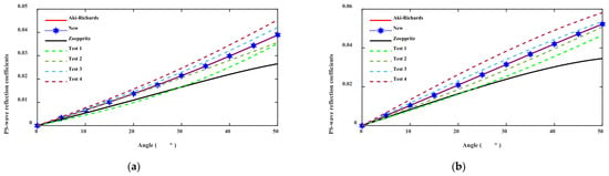
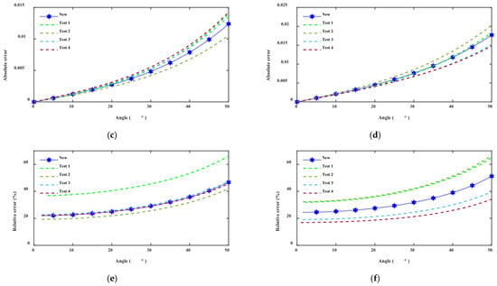
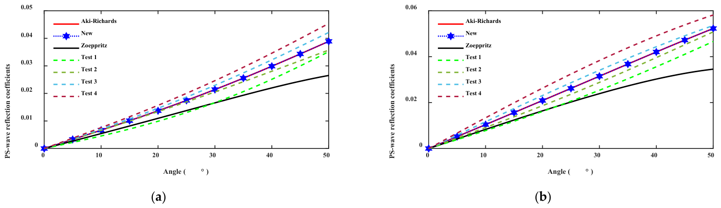
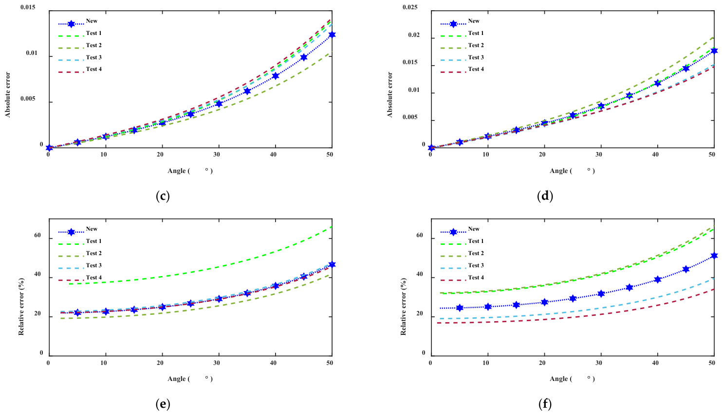
Figure 1a,b show responses over 0–50°. Black and red denote the unperturbed Zoeppritz and Aki–Richards results. Blue New overlaps the Aki–Richards results, confirming the equivalent local parameterization rather than improved accuracy. Tests 1–4 lie around the baseline, sometimes approaching or crossing the black curve. Figure 1c,d show the absolute difference between each approximate response and the Zoeppritz solution recalculated for that same perturbed interface. Figure 1e,f divide this difference by the magnitude of that case’s exact response and expresses it as a percentage. The unperturbed black curve is not the error reference for perturbed tests. Calculations use 0.5° increments, and absolute errors retain all angles.

Figure 1. PS reflection coefficient sensitivity and accuracy for Models 1 (left) and 2 (right). (a,b): original Table 1 baseline Aki–Richards (red), New formulation (blue hexagrams), exact Zoeppritz (black), and Tests 1–4 (colored dashed curves). (c,d): absolute approximation error relative to each case’s own exact Zoeppritz response. (e,f): corresponding relative error.

Approximation errors increase with angle, while their ranking depends on the model and perturbation. Over 0–30°, unperturbed PS-wave RMSE values are 0.002515 and 0.004071 for Models 1 and 2, respectively; test ranges are 0.002200–0.002880 and 0.003637–0.004524, respectively. Mean relative errors over eligible angles are 24.44% and 26.88% for the baselines, versus 21.41%–39.98% and 18.30%–35.57% for the tests, respectively. Therefore, the method exhibits a certain degree of robustness within the 0–30° range.

3.2. Synthetic-Data Test

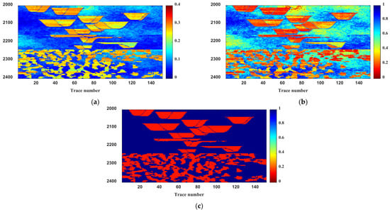
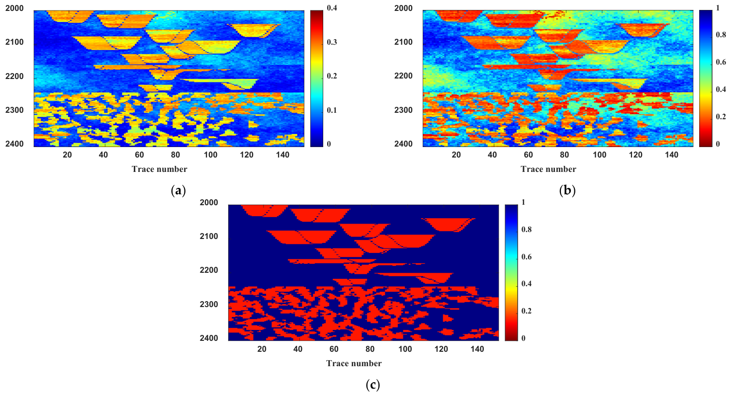
The performance of the proposed joint inversion framework is assessed using synthetic data generated from the Stanford VI-E model. In this model, clay volume is selected as the variable describing mineral composition. The true petrophysical models extracted along Inline = 100 are displayed in Figure 2.

Figure 2. Reference petrophysical models along Inline = 100: (a) porosity, (b) clay volume, and (c) water saturation.

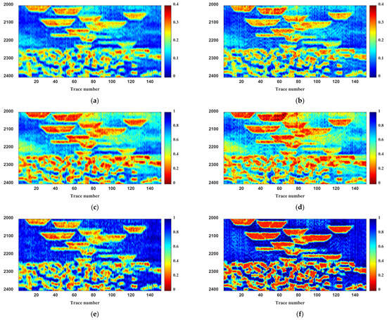
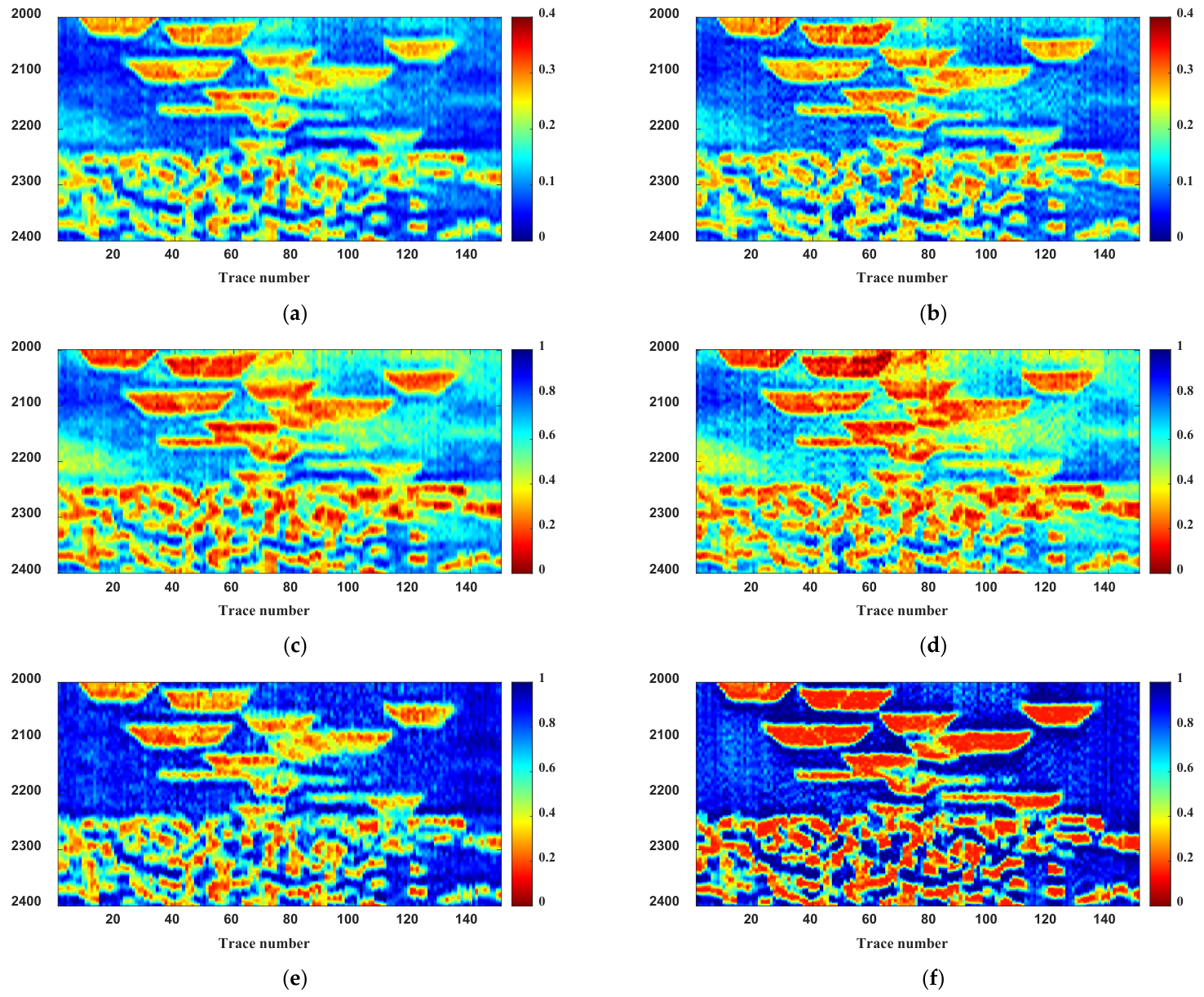
Two inversion experiments are performed for comparison. The first experiment uses PP-wave observations alone, whereas the second incorporates both PP- and PS-wave data within the proposed stochastic inversion framework. The resulting porosity, clay volume, and water saturation profiles along Inline = 100 are presented in Figure 3. At the scale resolved by the synthetic seismic data, both experiments reproduce the general distribution of the target properties, although the detailed structures remain insufficiently resolved when only the available seismic observations are considered.

Figure 3. Comparison of petrophysical parameter estimates obtained from PP-only and joint PP–PS inversion along Inline = 100: (a,c,e) PP-only results; (b,d,f) joint PP–PS results.

The inclusion of PS-wave observations introduces complementary sensitivity to the inversion, thereby providing additional constraints on the coupled petrophysical parameters. Compared with the PP-only case, the joint results preserve more of the fine-scale spatial variations and provide a clearer representation of the reservoir property distributions. The improvement is particularly evident in water saturation, for which the predicted values show a closer correspondence to the expected parameter range. Porosity and clay volume also benefit from the additional PS-wave constraints, with the joint inversion recovering more detailed variations than the corresponding PP-only results.

To prevent division by zero or very small true values, the revised relative error uses a denominator floor τ = 0.001 in fractional units (0.1 percentage point). The same regularized denominator is applied consistently to the model and the plotted profile.

$$R{E}_i={\displaystyle \frac{|{\widehat{x}}_i-x_i|}{\max (|x_i|,\tau )}}$$

(20)

where $R{E}_i$ denotes the displayed relative error at cell $i$, ${\widehat{x}}_i$ denotes the posterior-mean estimate, $x_i$ denotes the corresponding true value, $i$ indexes the cells in the Inline = 100 profile, and $\tau$ is the positive denominator floor, set to 0.001 in fractional units (0.1 percentage point). No true values in this profile fall below $\tau$, so the denominator floor leaves the original displayed error values unchanged.

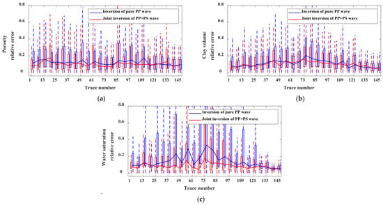
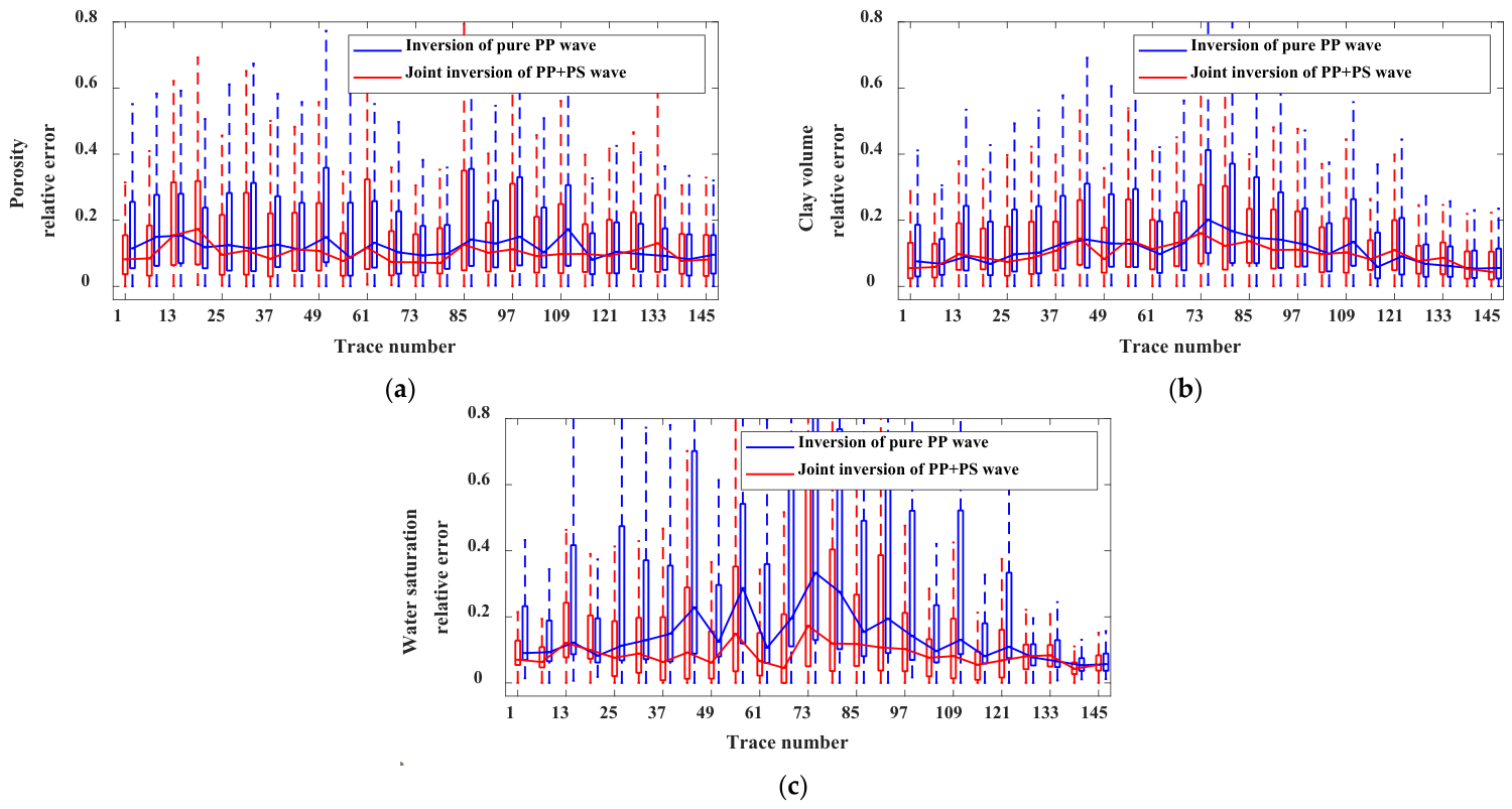
The spatial variation in inversion errors is further evaluated using the relative-error distributions shown in Figure 4. A total of 150 traces are included along the selected profile, and the error values are sampled every six traces to characterize their lateral variation. For porosity and clay volume, the joint PP–PS inversion generally produces smaller relative errors than the PP-only solution. The improvement is more pronounced for water saturation. After introducing the PS-wave observations, the corresponding errors are substantially reduced, particularly from trace 28 to trace 100, where the model contains strong vertical variations associated with the sandstone bodies.

Figure 4. Spatial distributions of relative errors along Inline = 100 for PP-only and joint PP–PS inversion. (a) Porosity relative error; (b) Clay volume relative error; (c) Water saturation relative error.

Table 3 presents the Mean Absolute Error (MAE), the Root Mean Squared Error (RMSE), and the correlation coefficient. Joint PP–PS inversion reduces water saturation MAE from 0.208 to 0.158 and RMSE from 0.247 to 0.222. Its correlation increases from 0.832 to 0.853. The MAE and RMSE values for porosity and clay volume derived from joint PP and PS wave inversion are lower than those from pure P-wave inversion, while the correlation coefficients are higher. Additionally, the accuracy of water saturation estimation is notably improved, a result that aligns with the relative errors shown in Figure 4.

Table 3. The Mean Absolute Error (MAE), the Root Mean Squared Error (RMSE), and the correlation coefficient.

Parameters	Inversion	MAE	RMSE	Correlation
Porosity	PP-only	0.035	0.050	0.843
	Joint PP–PS	0.034	0.049	0.851
Clay volume	PP-only	0.096	0.131	0.843
	Joint PP–PS	0.091	0.126	0.849
Water saturation	PP-only	0.208	0.247	0.832
	Joint PP–PS	0.158	0.222	0.853

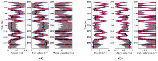
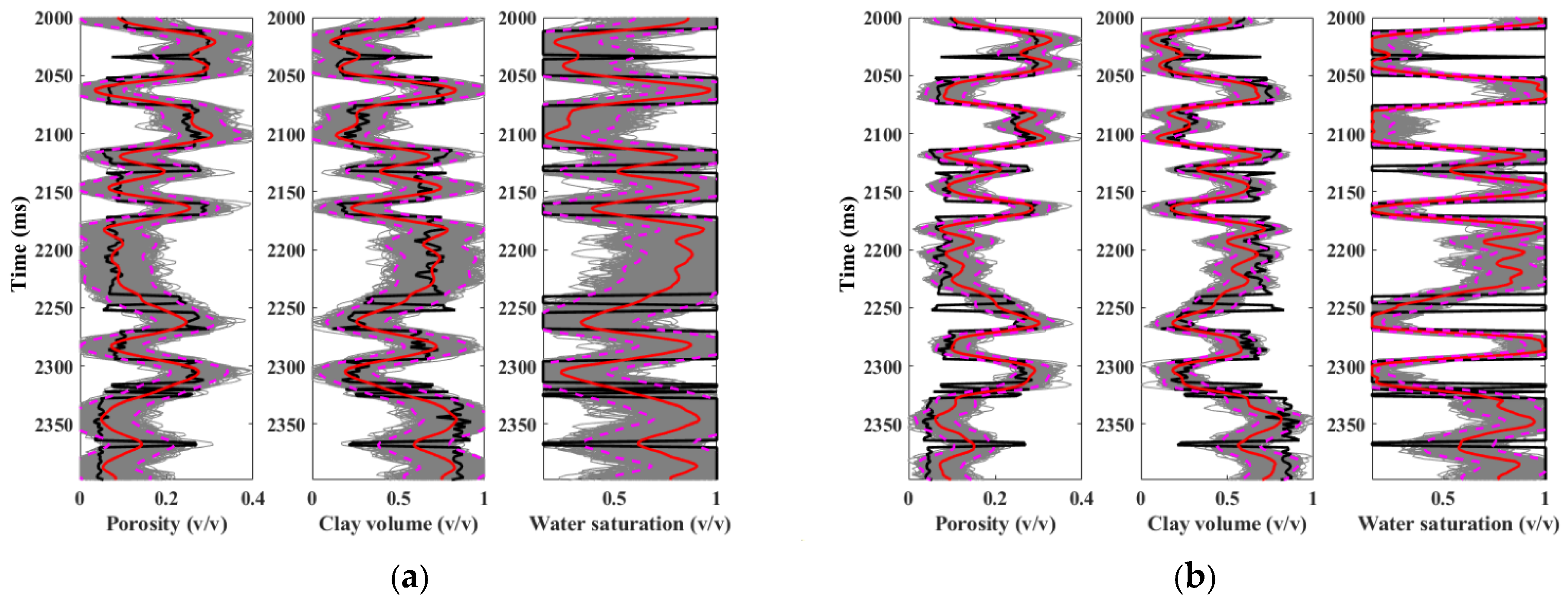
For the synthetic trace experiment, $N_e=500$, $N_a=4$, and ${\alpha }_k=4$ for all four steps. The 500 gray curves in Figure 5 are the final 500 ensemble members after the four assimilation steps, rather than 500 iterations or independent Markov-chain draws. The stopping rule is completion of the prescribed four assimilation steps. A more detailed assessment of the posterior uncertainty is carried out at trace 50, where the recovered parameters are compared directly with their corresponding true values (Figure 5). The inclusion of PS-wave information leads to a narrower posterior ensemble for the three petrophysical parameters. In most cases, the 95% confidence intervals also cover the reference models shown by the black curves, indicating that the additional PS-wave constraints reduce the uncertainty associated with the PP-only inversion.

Figure 5. Posterior petrophysical parameter estimates at Inline = 100 and Trace 50: (a) PP-only inversion; (b) joint PP–PS inversion. Black curves denote the reference models, gray curves represent 500 posterior realizations, red curves indicate the posterior means, and pink dashed lines mark the 95% confidence intervals.

The posterior means obtained from the two inversion schemes are then compared with the true parameter profiles. The Pearson correlation coefficients are calculated using all samples along this trace. For porosity, the coefficient increases from 0.837 for PP-only inversion to 0.848 for joint PP–PS inversion. For clay volume, it increases from 0.837 to 0.852, respectively. For water saturation, the coefficient increases from 0.829 to 0.849 respectively. The joint PP–PS solution provides closer estimates of the three petrophysical parameters and exhibits stronger correspondence with the reference models. Although the posterior-mean sections do not fully recover all fine-scale features, they reproduce the principal spatial variations in the three petrophysical properties.

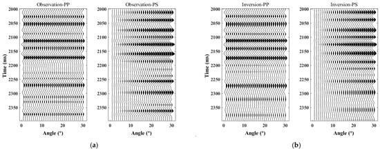
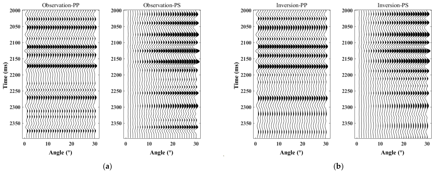
Finally, the consistency between the inversion results and the seismic observations is examined at Trace 50. Figure 6 illustrates the observed PP–PS seismic responses alongside those reproduced through forward modeling of the joint inversion results. Only minor discrepancies are observed between the two datasets, suggesting that the recovered petrophysical model provides an adequate explanation of the measured seismic responses.

Figure 6. Comparison between observed and reconstructed seismic data at Trace 50 from the joint PP–PS inversion: (a) observed seismic data; (b) reconstructed synthetic seismic data.

4. Field Data Example

A pre-stack seismic dataset from a Chinese oilfield is used to further examine the proposed PP–PS joint stochastic inversion approach under field conditions. The target interval is a gas-bearing dolomitic reservoir within the Qixia Formation. The seismic volume has a vertical sampling interval of 2 ms and covers Inline 1–399 and Crossline 1–400. Wells A, B, and C have all demonstrated relatively high and stable production during pilot testing, indicating favorable exploration potential of the Lower Permian Qixia Formation. Nevertheless, the target reservoirs are predominantly thin, which increases the difficulty of resolving their petrophysical characteristics accurately.

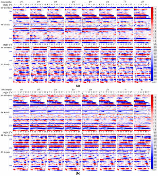
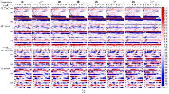
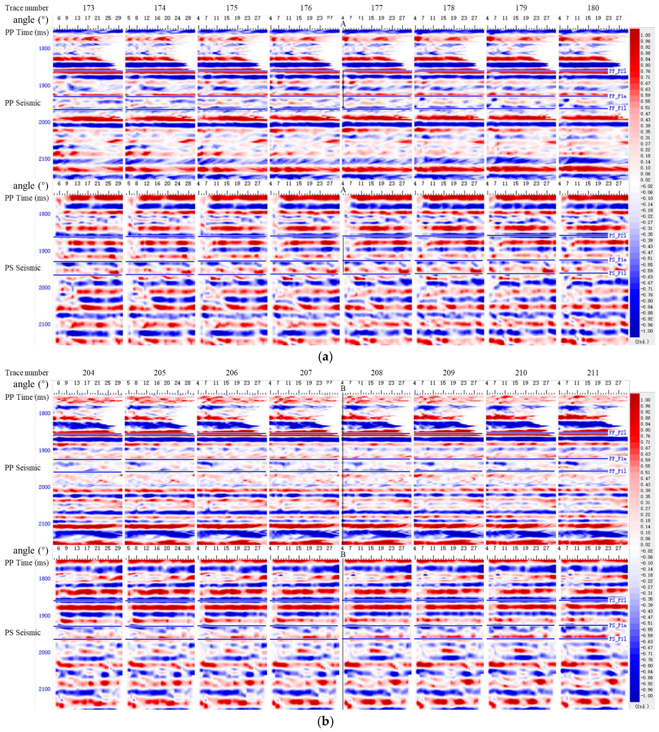
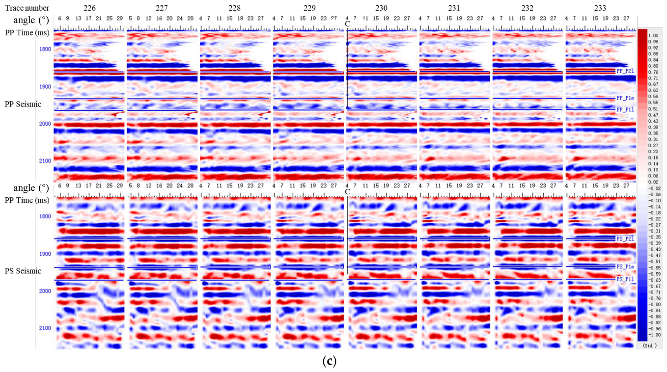
The angle gathers are first subjected to amplitude-preserving denoising so that the relative amplitude information can be retained. The two datasets are then aligned in the time domain, with the PS-wave gathers transformed to the PP-wave time reference. Examples of the resulting matched seismic sections are given in. Because the complete pre-stack angle-gather volume is extensive, only representative portions containing the traces close to the wells are displayed.

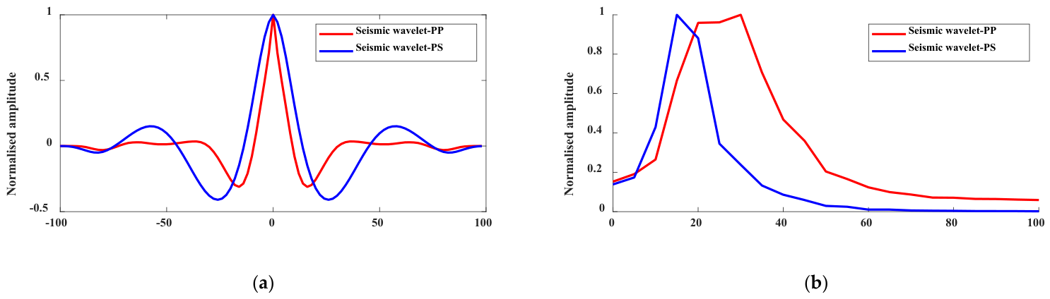
The three well locations used for the seismic-data comparison are marked in Figure 7. The section adjacent to Well A is located at Inline = 51, that of Well B at Inline = 352, and that of Well C at Inline = 175. Following time alignment, corresponding PP- and PS-wave events at the same stratigraphic boundary exhibit opposite polarities, with a PP-wave peak coinciding with a PS-wave trough. PP- and PS-wavelets are therefore extracted separately from the matched gathers. Because the two wavelets have opposite polarity, the PS-wavelet is phase-reversed here to facilitate direct comparison. Their time-domain waveforms and amplitude spectra are shown in Figure 8. The PP-wavelet has both a higher dominant frequency and a broader frequency bandwidth than the PS-wavelet. Wells A and B are subsequently used to condition the inversion, whereas Well C is reserved as an independent blind-well test.

Figure 7. Representative pre-stack angle gathers adjacent to the three wells: (a) Well A at Inline = 51; (b) Well B at Inline = 352; and (c) Well C at Inline = 175.

Figure 8. PP- and PS-wavelets and their amplitude spectra: (a) seismic wavelets; (b) corresponding frequency spectra.

The higher dominant frequency and broader bandwidth of the PP-wavelet provide finer temporal resolution, whereas the narrower PS-wave bandwidth can limit the recovery of thin-bed variations despite its complementary sensitivity to shear-related properties. The joint forward model uses the two wavelets separately, so their relative contributions depend on their spectral content, parameter sensitivities, and the adopted data-error covariance. Consequently, adding PS data may improve petrophysical constraints without resolving thin layers beyond the available bandwidth.

Core measurements were obtained primarily from Wells A and B. Data from these two wells were used to derive the statistics for the linearized rock physics model. The porosity of the dolomitic reservoir is concentrated mainly between 2% and 5%, with a mean of 3.87% and a median of 3.37%. With a median value of just 0.022 × 10⁻³ μm², the permeability underscores the reservoir’s low-porosity and ultra-low-permeability character. Elastically, the high-quality zones at Wells A, B, and C exhibit relatively low P-wave velocity, paired with elevated S-wave velocity and density. These zones also display low gamma-ray and resistivity values in their petrophysical signatures. Collectively, these findings further support the exploration potential of the Lower Permian Qixia Formation. The relatively high bulk density can be consistent with the dolomite-dominated mineral framework and the low porosity reported above. Bulk density reflects both the solid matrix and the pore fluids, and at a porosity of only 2%–5%, the mineral framework dominates the response. In heterogeneous carbonates, saline water retained in connected micropores can maintain conductive pathways while hydrocarbons occupy larger pores. Thin-bed averaging can also reduce the measured resistivity contrast [35].

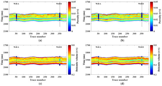
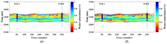
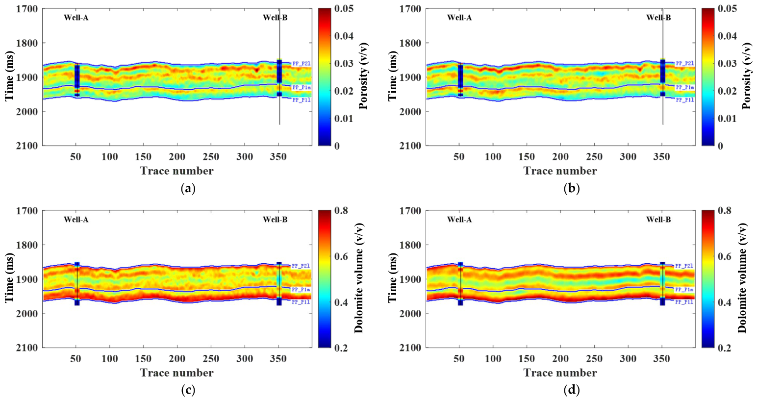
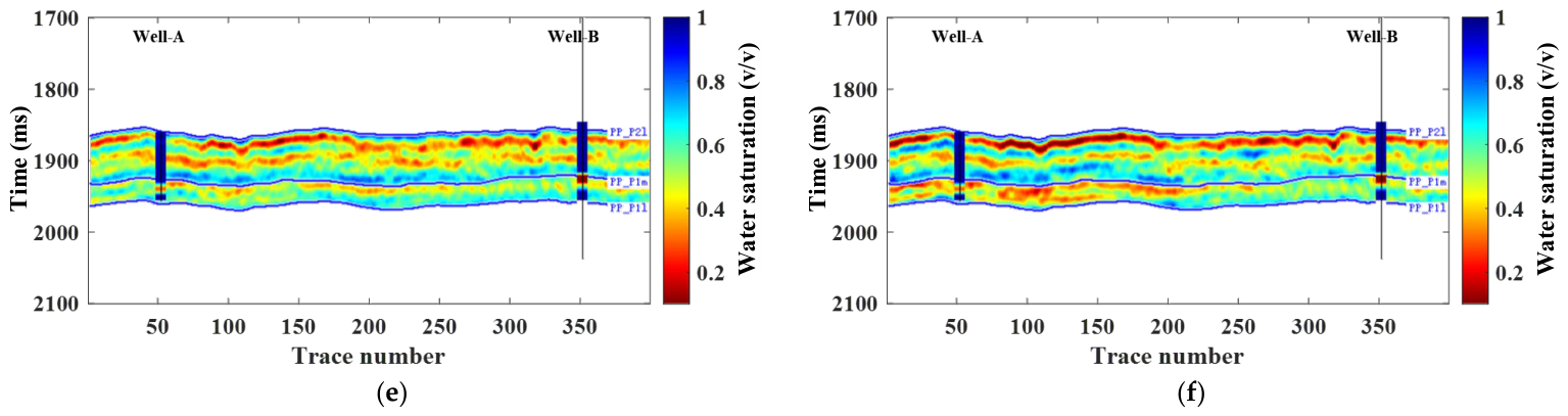
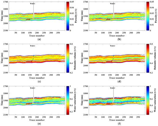
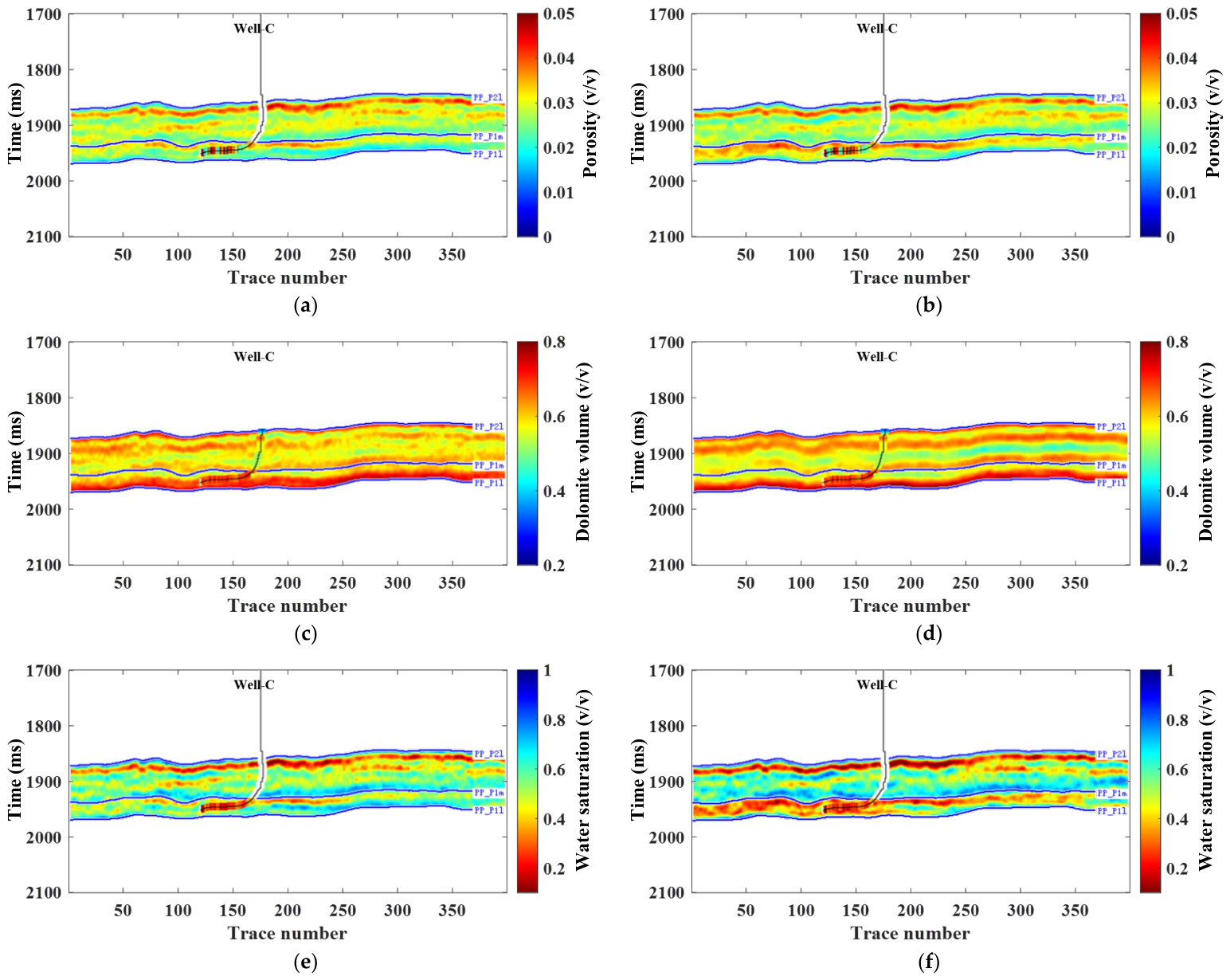
Because dolomite constitutes the dominant reservoir lithology in the study area, dolomite volume is adopted as the mineral-related variable. The field data are then inverted using two configurations: PP-wave observations alone and the combined PP–PS dataset, with both schemes incorporating statistically derived priors. The resulting sections along Crossline = 177 are presented in Figure 9, where porosity, dolomite volume, and water saturation are compared between the two inversion cases. The correlations for Well A are 0.66 and 0.71 for porosity, 0.68 and 0.69 for dolomite volume, and 0.62 and 0.68 for water saturation for PP-only and joint PP–PS inversion, respectively. At Well B, the corresponding correlations are 0.67 and 0.70, 0.61 and 0.66, and 0.56 and 0.61, respectively.

Figure 9. Petrophysical parameter sections along Crossline = 177 obtained from PP-only and joint PP–PS inversion: (a,c,e) porosity, dolomite volume, and water saturation from PP-only inversion. (b,d,f) corresponding joint inversion results.

The high-porosity zones recovered from the inversion coincide with the interpreted gas-bearing reservoir intervals. At Well A, the porosity profile obtained from the PP–PS solution follows the measured well data more closely than the PP-only result. The inverted dolomite volume also increases within the target reservoir intervals, although noticeable discrepancies remain between the seismic estimates and the well measurements for both inversion schemes. Water saturation is generally lower within the gas-bearing zones. At Well A, its PP–PS estimate shows better agreement with the well observation, whereas the difference between the two inversion results is relatively limited at Well B.

The independent blind-well test provides a further check on the predictive capability of the inversion. Figure 10 shows the petrophysical sections crossing Well C at Crossline = 230, with the PP-only estimates and the joint PP–PS estimates displayed for comparison. The correlations for PP-only and joint PP–PS inversion are 0.57 and 0.63 for porosity, 0.53 and 0.58 for dolomite volume, and 0.52 and 0.60 for water saturation, respectively. In the vicinity of the blind well, the recovered porosity is relatively high, and the joint solution agrees more closely with the measured porosity than the PP-only result. Dolomite volume is likewise elevated in this interval, consistent with the pattern observed at the conditioning wells, although neither inversion completely reproduces the well measurement. Water saturation remains relatively low around the blind well, and the PP–PS result again shows closer correspondence with the observation. Across the entire sections, the recovered petrophysical models retain strong lateral continuity, which can be attributed to the constraints imposed by statistically derived parameter priors.

Figure 10. Petrophysical parameter sections along Crossline = 230 across the blind well: (a,c,e) PP-only estimates of porosity, dolomite volume, and water saturation. (b,d,f) corresponding joint PP–PS estimates.

5. Conclusions

To address the substantial uncertainty arising from multiparameter coupling in PP-wave-only inversion, this study developed a rock-physics-constrained PP–PS joint stochastic inversion method for petrophysical parameter prediction. The proposed method jointly constrains key reservoir petrophysical parameters by integrating multi-wave seismic information. By establishing statistical rock physics relationships, porosity, mineral content, and water saturation are selected as the target inversion parameters, and the corresponding linearized PS-wave reflection coefficient equation is derived. Interface reflection response analysis demonstrates that the proposed approximation equation has good applicability within the typical range of reservoir parameter variations. This equation also provides a theoretical basis for joint P- and S-wave inversion.

Within this framework, a joint stochastic inversion equation with petrophysical parameters as direct unknown variables is constructed, and PP- and PS-wave data are jointly inverted to estimate petrophysical parameters. Synthetic tests based on the Stanford VI-E model demonstrate that incorporating PS-wave information yields petrophysical parameter estimates closer to the true model, reduces uncertainty, and improves inversion accuracy compared with PP-wave-only inversion.

Application to real multicomponent pre-stack seismic data yields PP–PS joint stochastic inversion results with lateral continuity in the displayed sections. The inverted petrophysical parameters reproduce the main reservoir-scale variations indicated by well data, although local discrepancies remain. Together, the theoretical derivation and the synthetic and field examples indicate that joint PP–PS stochastic inversion has potential for subsurface petrophysical estimation, although further quantitative validation is warranted. Further validation using additional independent wells and datasets is needed to assess its predictive performance and applicability to other reservoirs. The framework relies on linearized rock physics relationships and isotropic reflection approximations, so strong property contrasts or appreciable anisotropy may require a more general forward model.

References

- Liu, Z.W.; Sa, L.M.; Yang, X.; Li, X.Y. Needs of geophysical technologies for shale gas exploration. Oil Geophys. Prospect. 2011, 46, 810–818. [Google Scholar]
- Singh, K.; Holditch, S.A.; Ayers, J.W.B. Basin analog investigations answer characterization challenges of unconventional gas potential in frontier basins. J. Energy Resour. Technol. 2008, 130, 043202–043207. [Google Scholar] [CrossRef] [Scilit]
- Bouchaala, F.; Guennou, C. Estimation of viscoelastic attenuation of real seismic data by use of ray tracing software: Application to the detection of gas hydrates and free gas. Comptes Rendus. Géosci. 2012, 344, 57–66. [Google Scholar] [CrossRef] [Scilit]
- Zong, Z.Y.; Yin, X.Y.; Wu, G.C. AVO inversion and poroelasticity with P-and S-wave moduli. Geophysics 2012, 77, N17–N24. [Google Scholar] [CrossRef] [Scilit]
- Hou, D.J. PP and PS AVO joint inversion for P- and S-wave moduli based on Bayes theorem. In Proccedings of the SEG International Exposition and Annual Meeting 2017, Houston, TX, USA, 24–29 September 2017. SEG-2017-17798920. [Google Scholar]
- Bouchaala, F.; Ali, M.Y.; Matsushima, J. Compressional and shear wave attenuations from walkway VSP and sonic data in an offshore Abu Dhabi oilfield. Comptes Rendus. Géosci. 2021, 353, 337–354. [Google Scholar] [CrossRef] [Scilit]
- Stewart, R.R. Joint P and P-SV inversion. In The CREWES Project Research Report; Consortium for Research in Elastic Wave Exploration Seismology: Calgary, AB, Canada, 1990; Volume 2, pp. 112–115. [Google Scholar]
- Larsen, J.A. AVO Inversion by Simultaneous P-P and P-S Inversion; University of Calgary: Calgary, AB, Canada, 1999. [Google Scholar]
- Margrave, G.F.; Stewart, R.R.; Larsen, J.A. Joint PP and PS seismic inversion. Lead. Edge 2001, 20, 1048–1052. [Google Scholar] [CrossRef] [Scilit]
- Chen, T.S.; Liu, Y.; Wei, X.C. Joint amplitude versus offset inversion of P-P and P-SV seismic data. J. China Univ. Pet. 2006, 30, 33–37. [Google Scholar]
- Hu, G.Q.; Liu, Y.; Wei, X.C.; Chen, T.S. Joint PP and PS AVO inversion based on Bayes theorem. Appl. Geophys. 2011, 8, 293–302. [Google Scholar] [CrossRef] [Scilit]
- Luo, C.; Ba, J.; Carcione, J.M.; Huang, G.T.; Guo, Q. Joint PP and PS pre-stack seismic inversion for stratified models based on the propagator matrix forward engine. Surv. Geophys. 2020, 41, 987–1028. [Google Scholar] [CrossRef] [Scilit]
- Luo, C.; Ba, J.; Carcione, J.M. A hierarchical prestack seismic inversion scheme for VTI media based on the exact reflection coefficient. IEEE Trans. Geosci. Remote Sens. 2022, 60, 4507416. [Google Scholar] [CrossRef] [Scilit]
- Zhi, L.X.; Chen, S.Q.; Li, X.Y. Joint AVO inversion of PP and PS waves using exact Zoeppritz equation. In Proceedings of the SEG International Exposition and Annual Meeting 2013, Houston, TX, USA, 22–27 September 2013; pp. 457–461. [Google Scholar]
- Lu, J.; Yang, Z.; Wang, Y.; Shi, Y. Joint PP and PS AVA seismic inversion using exact Zoeppritz equations. Geophysics 2015, 80, R239–R250. [Google Scholar] [CrossRef] [Scilit]
- Li, L.M.; Luo, S.X.; Wang, M.C.; Kong, X.L.; Zhou, H.L. 3D PP-PS joint inversion method and application in anisotropic medium. Oil Geophys. Prospect. 2010, 45, 60–65. [Google Scholar]
- Zhang, G.Z.; Du, B.Y.; Li, H.S.; Chen, H.Z.; Li, Z.Z.; Yin, X.Y. The method of joint pre-stack inversion of PP and P-SV waves in shale gas reservoirs. Chin. J. Geophys. 2014, 57, 4141–4149. (In Chinese) [Google Scholar]
- Gong, X.P.; Zhang, F.; Li, X.Y.; Chen, S.Q. Study of S-wave ray elastic impedance for identifying lithology and fluid. Appl. Geophys. 2013, 10, 145–156. [Google Scholar] [CrossRef] [Scilit]
- Zhang, F.; Li, X.Y. Inversion of the reflected SV-wave for density and S-wave velocity structures. Geophys. J. Int. 2020, 221, 1635–1639. [Google Scholar] [CrossRef] [Scilit]
- Luo, C.; Li, X.Y.; Huang, G.T. Information on S-wave velocity and density obtained from multiwave data. In Proceedings of the SEG International Exposition and Annual Meeting 2018, Anaheim, CA, USA, 14–19 October 2018; pp. 2412–2416. [Google Scholar]
- Zhang, F. Simultaneous inversion for S-wave velocity and density from the SV-SV wave. Geophysics 2021, 86, R187–R195. [Google Scholar] [CrossRef] [Scilit]
- Dai, F.; Zhang, F.; Li, X.Y. SH-SH wave inversion for S-wave velocity and density. Geophysics 2022, 87, A25–A32. [Google Scholar] [CrossRef] [Scilit]
- Bouchaala, F.; Ali, M.Y.; Matsushima, J. Attenuation modes from vertical seismic profiling and sonic waveform in a carbonate reservoir, Abu Dhabi, United Arab Emirates. Geophys. Prospect. 2016, 64, 1030–1047. [Google Scholar] [CrossRef] [Scilit]
- Zhou, Z.S. AVO analysis of P-SV and SH wave. Oil Geophys. Prospect. 1993, 28, 430–438. [Google Scholar]
- Gomez, C.T.; Tatham, R.H. Sensitivity analysis of seismic reflectivity to partial gas saturation. Geophysics 2007, 72, C45–C57. [Google Scholar] [CrossRef] [Scilit]
- Gupta, M.; Hardage, B. SV-P: A potential viable alternative to mode-converted P-SV seismic data for reservoir characterization. Interpretation 2017, 5, T579–T589. [Google Scholar] [CrossRef] [Scilit]
- Gupta, M.; DeAngelo, M.V.; Hardage, B. PP and SS wave interpretation of a carbonate formation: A case study from the Arbuckle interval in Wellington field, Kansas. In Proceedings of the SEG International Exposition and Annual Meeting 2015, New Orleans, LA, USA, 18–23 October 2015. SEG-2015-5834398. [Google Scholar]
- Roure, B.; Russell, B. A preliminary look at joint PP-PS-SS inversion in native time domain. In Proceedings of the SEG International Exposition and Annual Meeting 2019, San Antonio, TX, USA, 15–20 September 2019; pp. 5370–5374. [Google Scholar]
- Lin, Y.; Zhang, G.Z.; Wang, B.L.; Zhu, Z.Y.; Gao, J.H. Multi-wave Stochastic Inversion Physical Parameters Prediction Method Driven by Linearized Rock Physics. IEEE Trans. Geosci. Remote Sens. 2024, 62, 1–14. [Google Scholar] [CrossRef] [Scilit]
- Yin, X.Y.; Cui, W.; Zong, Z.Y.; Liu, X.J. Petrophysical property inversion of reservoirs based on elastic impedance. Chin. J. Geophys. 2014, 57, 4132–4140. (In Chinese) [Google Scholar]
- Grana, D. Bayesian linearized rock-physics inversion. Geophysics 2016, 81, D625–D641. [Google Scholar] [CrossRef] [Scilit]
- Kenter, J.A.M.; Podladchikov, F.F.; Reinders, M.; Van der Gaast, S.J.; Fouke, B.W.; Sonnenfeld, M.D. Parameters controlling sonic velocities in a mixed carbonate-siliciclastics Permian shelf-margin (upper San Andres formation, Last Chance Canyon, New Mexico). Geophysics 1997, 62, 505–520. [Google Scholar] [CrossRef] [Scilit]
- Dvorkin, J.P. Yet another VS equation. Geophysics 2008, 73, E35–E39. [Google Scholar] [CrossRef] [Scilit]
- Emerick, A.A.; Reynolds, A.C. Ensemble smoother with multiple data assimilation. Comput. Geosci. 2013, 55, 3–15. [Google Scholar] [CrossRef] [Scilit]
- Awolayo, A.; Ashqar, A.; Uchida, M.; Salahuddin, A.A.; Olayiwola, S.O. A cohesive approach at estimating water saturation in a low-resistivity pay carbonate reservoir and its validation. J. Pet. Explor. Prod. Technol. 2017, 7, 637–657. [Google Scholar] [CrossRef] [Scilit]
Disclaimer/Publisher’s Note: The statements, opinions and data contained in all publications are solely those of the individual author(s) and contributor(s) and not of MDPI and/or the editor(s). MDPI and/or the editor(s) disclaim responsibility for any injury to people or property resulting from any ideas, methods, instructions or products referred to in the content. |
© 2026 by the authors. Licensee MDPI, Basel, Switzerland. This article is an open access article distributed under the terms and conditions of the Creative Commons Attribution (CC BY) license.