Hybrid Linear–Nonlinear Model with Adaptive Regularization for Accurate X-Ray Fluorescence Determination of Total Iron Ore Grade

Abstract

In mineral processing and metallurgy, total iron grade serves as a critical indicator guiding the entire production chain from crushing to smelting, directly influencing the quality and yield of steel products. To address the limitations of conventional matrix effect correction methods in X-ray fluorescence (XRF) analysis—such as low accuracy, high time consumption, and labor-intensive procedures—this study proposes a novel hybrid model (DSCN-LS) integrating least squares (LS) with dynamically regularized stochastic configuration networks (DSCNs) for total iron ore grade quantification. Through feature analysis, we decompose the grade modeling problem into a linear structural component and nonlinear residual terms. The linear component is resolved by means of LS, while the nonlinear terms are processed by the DSCN with a dynamic regularization strategy. This strategy implements node-specific weighted regularization: weak constraints preserve salient features in high-weight-norm nodes, while strong regularization suppresses redundant information in low-weight-norm nodes, collectively enhancing model generalizability and robustness. Notably, the model was trained and validated using datasets collected directly from industrial sites, ensuring that the results reflect real-world production scenarios. Industrial validation demonstrates that the proposed method achieves an average absolute error of 0.3092, a root mean square error of 0.5561, and a coefficient of determination (R²) of 99.91% in total iron grade estimation. All metrics surpass existing benchmarks, confirming significant improvements in accuracy and operational practicality for XRF detection under complex industrial conditions.

1. Introduction

The mining and processing industry is of pivotal significance to the modern economy. The accurate measurement of iron content in ores has a direct impact on resource utilization and production costs. In the realm of analytical methodologies, X-ray fluorescence spectroscopy (XRF) has emerged as a prevalent technique for mineral composition analysis. This method’s preeminence can be attributed to its non-destructive nature and expeditious nature [1]. However, when employing XRF technology for quantitative analysis of elements in samples, it is often challenging to obtain accurate results due to several influencing factors, including absorption–enhancement effects among elements, particle size variations, and mineral effects. The components in the sample other than the analyzed elements are collectively referred to as the matrix. If the matrix composition of the sample under test is complex, the absorption–enhancement effects between elements become notably pronounced. Among these factors, the matrix effect stands out as the primary challenge encountered by engineers using XRF technology for quantitative analysis. These interactions are inherently nonlinear, as the fluorescence intensity of the target element is influenced not only by its own concentration but also by the simultaneous absorption and secondary excitation effects of other elements in the sample matrix. This inter-element coupling gives rise to complex nonlinear dependencies.

Traditional XRF detection methods [2,3,4] mainly depend on empirical models and instrument calibration with basic parameter approaches. Their main goal is to model linear relationships between individual elements and their X-ray fluorescence signals [5]. However, in real-world ore samples, multiple matrix elements interact, creating complex matrix effects that greatly reduce detection accuracy. Additionally, these traditional methods mainly use linear regression models, which cannot capture nonlinear interactions between elements, leading to accumulated errors. These technical limits are especially noticeable in industrial settings for iron ore grade detection, particularly in complex and dynamic environments at mineral processing sites, where the weaknesses of conventional XRF techniques become even clearer. In this context, ‘complex industrial environments’ refers to scenarios where sample preparation and handling involve multiple processing steps, each of which may introduce operational errors, and where conventional manual laboratory methods are time-consuming, labor-intensive, and involve cumbersome procedures. These factors collectively create additional challenges for accurate, efficient, and sustainable XRF analysis, making the weaknesses of conventional techniques even more pronounced.

Recently, with the rapid progress of artificial intelligence (AI) technology, machine learning (ML) based detection methods [6,7,8,9,10] have become a promising way to overcome the limits of traditional XRF methods. By using nonlinear modeling and feature learning [11], ML approaches show great potential for analyzing complex ore samples. Wang et al. [12] proposed a hybrid correction strategy that combines mechanical XRF methods with data-driven techniques, pairing the least squares method with block incremental stochastic configuration networks (BIRCNs). They introduced a Fisher information matrix compression model to optimize model size, improving the accuracy and efficiency of titanium iron ore grade prediction. However, its static model compression and iterative expansion increase computational cost and limit adaptability to varying industrial conditions. Zhang et al. [13] created a method to quantify heavy metal elements (HMEs) in soil by combining XRF with deep learning, aiming to boost analytical accuracy under complex matrix conditions. They designed a feature mining collaboration module and a deep spectral prediction network (DSPFormer) to accurately estimate five elements: Ti, Mn, Cu, Zn, and Pb. Nonetheless, current machine learning-based XRF analysis methods still face key issues: High-noise industrial environments often lead to poor feature selection and inefficient nonlinear compensation, which causes unstable model performance. Traditional single-model architectures [14] struggle to balance the interpretability of linear models with nonlinear interference modeling, limiting further improvements in detection accuracy. As a result, existing XRF–machine learning hybrid models still cannot effectively handle nonlinear matrix effects under industrial noise, restricting both model stability and detection accuracy.

In response to the aforementioned challenges, this study proposes an X-ray fluorescence (XRF) detection method for total iron ore grade that integrates dynamically regularized stochastic configuration networks (DSCN) with the least squares (LS) technique. The proposed approach combines the feature selection capability of the alternating direction method of multipliers (ADMM) and Lasso regression [15] with the nonlinear modeling capability of the DSCN, enabling accurate and adaptive determination of total iron grade in ores under complex matrix conditions. Compared with traditional empirical analysis and basic parameter-based calibration methods, the proposed method substantially improves detection accuracy—achieving a 35% reduction in RMSE—and demonstrates enhanced robustness under complex industrial conditions. Furthermore, it exhibits strong generalization capability and adaptability for real-world applications. However, the method involves relatively high computational costs during model training and optimization due to the nonlinear network structure and iterative regularization process.

2. Feature Analysis of Total Iron Ore Grade Modeling Based on XRF

2.1. Working Principle of XRF Spectrometer

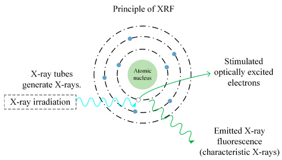
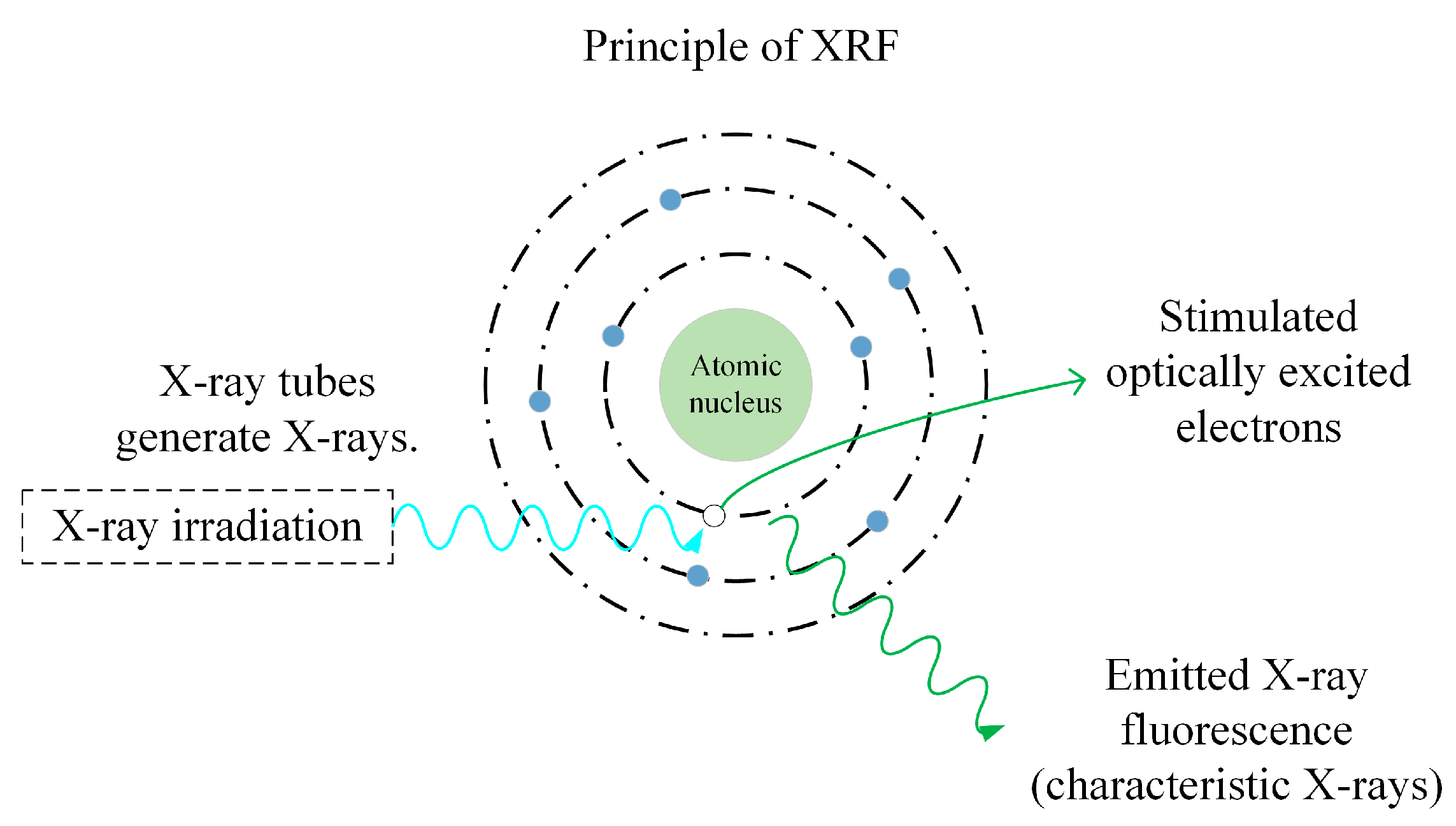
X-ray fluorescence spectroscopy is an analytical technique based on characteristic X-ray excitation and emission. The fundamental principle underlying this process is the utilization of X-rays or radioactive nuclides as the excitation source. When the sample is excited, the inner electrons of the atoms are knocked out, forming holes and causing the atoms to become excited. Subsequently, outer-shell electrons fill the holes by transitioning to inner shells. During this process, electrons transition from higher energy levels to lower energy levels, releasing excess energy in the form of characteristic X-rays. This results in the formation of X-ray fluorescence spectra with specific energies. It is evident that atoms of differing elements possess distinct energy level structures. Consequently, under equivalent excitation conditions, the characteristic X-ray energy produced by electron transitions between inner atomic shells exhibits a strict correlation with the atomic number of the element. This one-to-one correspondence between energy and element type facilitates qualitative and quantitative analysis of elements in a sample by detecting the energy of characteristic X-rays. The overall principle of this mechanism is illustrated in Figure 1.

Figure 1. Principle of XRF.

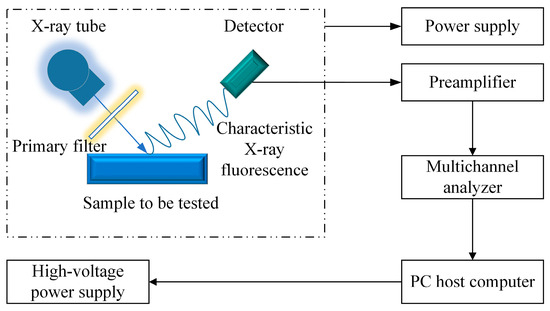
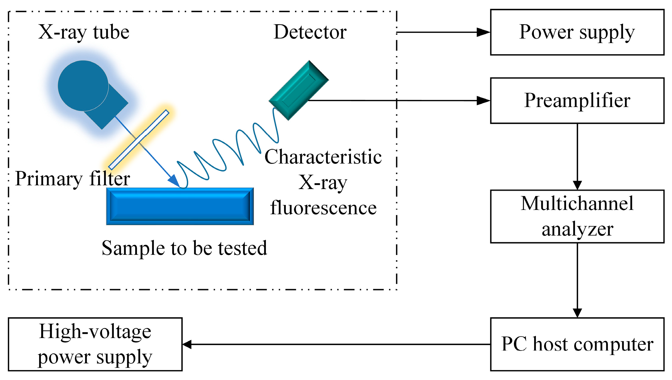
The Energy-Dispersive X-ray Fluorescence (EDXRF) system [16,17,18] is based on the fundamental principle of the interaction between X-rays and matter. The system generally includes a power supply module, X-ray source, detector, collimator, filter, amplification circuit, and a host computer. The power supply provides the necessary electrical energy for all components, with the high-voltage unit responsible for generating continuous spectrum X-rays in the X-ray tube. These primary X-rays are directed onto the sample surface through a collimator and filter to ensure beam accuracy and minimize background noise. When irradiated, the elements within the sample are excited and emit characteristic X-rays, which are then captured by the detector. The detector converts the incoming photons into pulse signals. These signals are amplified by the front-end amplification circuit. After amplification, the analog signals are digitized and collected for further analysis. The data is then transmitted to the host computer, where specialized software performs spectral analysis and determines the elemental composition. Figure 2 shows a schematic diagram of the EDXRF system architecture. In the present study, XRF is applied to measure the fluorescence intensity of key elements in total iron ore samples, including Si, Fe, Ca, and SiO₂. These measured intensities serve as the input features for the regression models used to predict the total iron grade. By providing rapid and non-destructive elemental analysis under industrial conditions, XRF enables accurate characterization of ore composition and supports the construction of both the preliminary grade estimation model and the correction compensation model described in Section 3.

Figure 2. EDXRF system structure diagram.

By detecting the intensity of these characteristic X-rays, the content of each element in the sample can be determined. In ore grade testing, XRF technology provides the advantages of non-destructive and rapid analysis. However, the presence of multiple elements in ore samples can cause complex matrix effects that impact the accuracy of test results.

2.2. Principles and Processes of Total Iron Ore Grade Testing

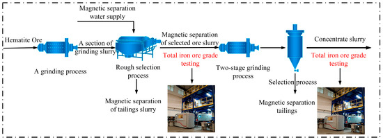
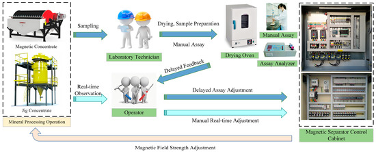
Total iron ore grade testing covers a broad area and is a crucial part of production. A flow chart of a “two-stage grinding-multi-stage separation” total iron ore beneficiation process [19,20] is shown in Figure 3. The iron ore first undergoes a single stage of grinding to reduce it to a particle size suitable for magnetic separation. The ground ore slurry then goes to the roughing magnetic separator for initial iron mineral recovery. After rough magnetic separation, the magnetic concentrate slurry moves to a second stage of grinding for finer grinding to free more iron minerals embedded in the ore, followed by a concentrating stage for high-precision separation to produce high-grade concentrate. Among these key steps, it is especially important to install a detection system for total iron ore grade, particularly after rough and fine separation processes. This system continuously measures the actual iron content in the slurry, enabling dynamic monitoring and precise control of the process. Compared with traditional manual sampling and testing, such testing not only increases testing frequency and accuracy but also prevents production losses caused by human error and testing delays. Nevertheless, conventional detection methods are often limited by slower response times, reduced adaptability to complex slurry compositions, and dependence on manual calibration. These limitations have driven the development of intelligent detection approaches, which employ advanced data-driven models to deliver faster, more accurate, and adaptive predictions of total iron ore grade, thereby enhancing the efficiency, reliability, and overall performance of the beneficiation process.

Figure 3. Two-stage grinding—multi-stage separation.

2.3. Problem Description of Total Iron Ore Grade Detection

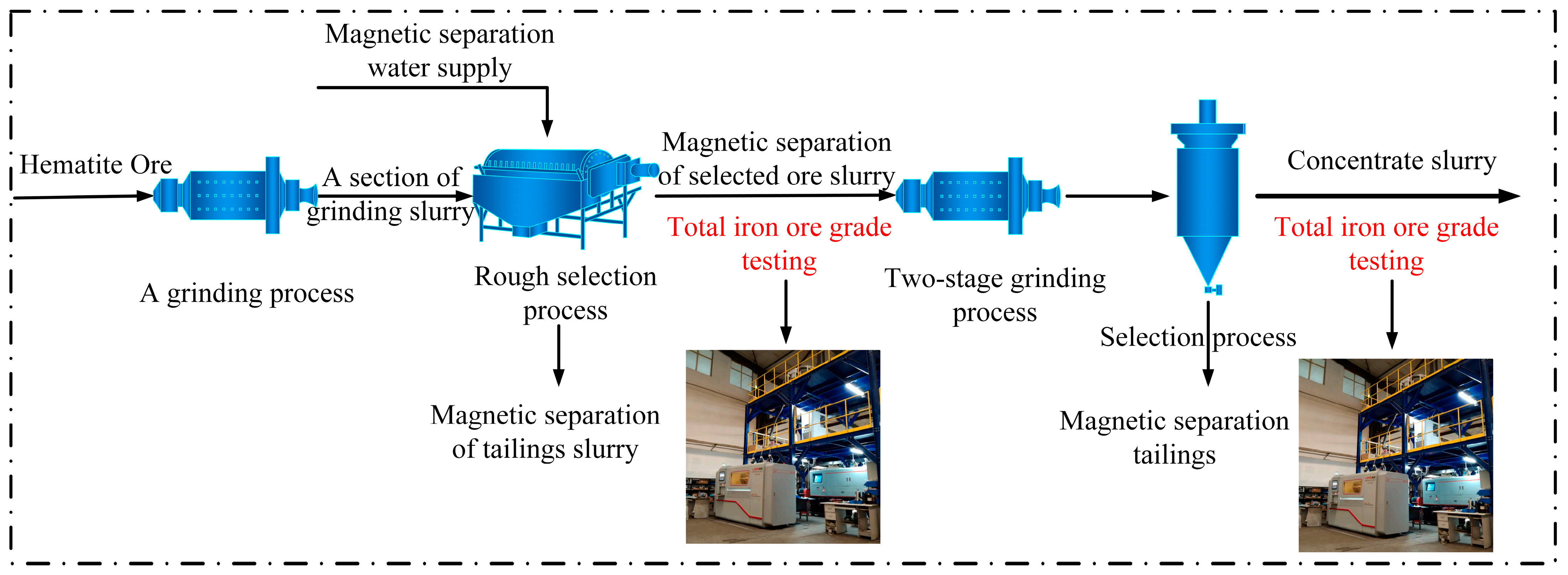
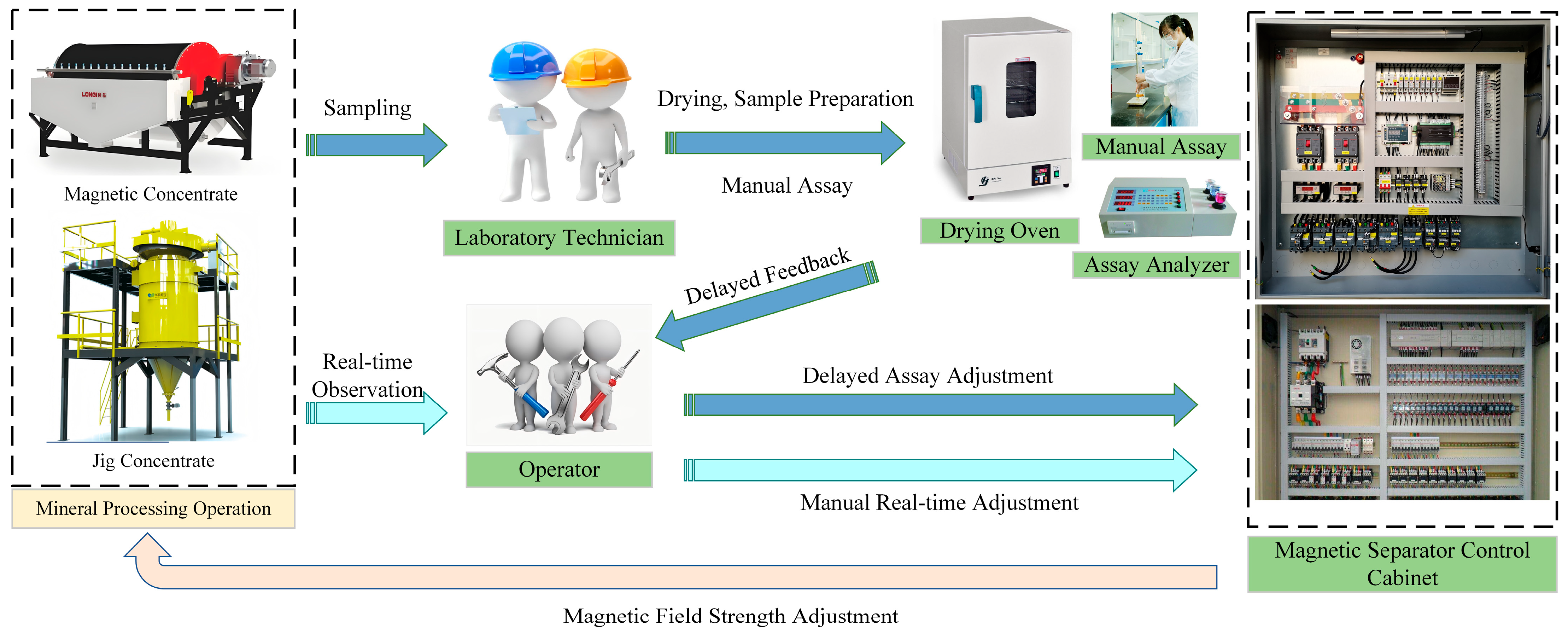
In traditional ore dressing processes, mineral grade detection [21,22,23] serves as a critical control link, where the accuracy and real-time performance of detection directly impact the efficiency of ore dressing and the recovery rate of resources. As shown in Figure 4, current production practices primarily rely on a combination of manual experience-based judgment and laboratory analysis for parameter adjustment. Operators monitor the morphology of flotation froth from the magnetic separator and changes in tailings color in real time, adjusting key parameters such as the field strength of the jig machine based on their experience. While this method offers rapid response capabilities, it is constrained by the limitations of human expertise, being susceptible to factors such as the operator’s skill level and subjective judgment biases. Meanwhile, laboratory technicians conduct standardized pretreatment (including drying and sample preparation) on sampled ores, utilizing ovens and grade analyzers to determine the mineral grade. The test results are then fed back to the operational end to guide subsequent adjustments. Although this approach provides high-precision grade data, the prolonged sampling cycle (typically ranging from several hours to days) and complex pretreatment procedures result in significant time delays between the test outcomes and actual production conditions. This may lead to missed optimal control windows, thereby increasing energy consumption and resource losses. Furthermore, the traditional detection model struggles to achieve multi-parameter collaborative control, as there is a lack of dynamic coupling mechanisms between the field strength adjustment of magnetic separators, operational parameters of the jig machine, and grade detection data, which hinders the intelligent and refined development of ore dressing processes.

Figure 4. Manual Control System Diagram for Magnetite Separation.

2.4. Modeling Feature Analysis

In the early 20th century, Moseley discovered that different elements emit X-ray fluorescence with characteristic frequencies when excited by X-rays, and that these frequencies have a stable functional relationship with the atomic number $Z$ of the elements [24]. (1) expresses Moseley’s law.

$$v=C_1{(Z-\sigma )}^2$$

(1)

where $v$ is the frequency of characteristic X-ray fluorescence, $C_1$ is a constant, $Z$ is the atomic number of the element, $\sigma$ is the shielding constants, reflecting the shielding effect of inner electrons. It is evident that in (2), the frequency of elemental characteristic X-ray fluorescence is proportional to the square of the atomic number. According to the equation for calculating the photon energy in each X-ray:

$$E=hv$$

(2)

where $E$ is the energy of the X-ray photon, the Planck constant $h$ is typically taken as $h\approx 6.626\times {10}^{-34}\mathrm{J}\cdot \mathrm{s}$.

Combining (1) and (2), we can obtain (3):

$$E=h{C}_1{(Z-\sigma )}^2=C_2{(Z-\sigma )}^2$$

(3)

where $C_2=h{C}_1$ is a constant. It can thus be seen that the X-ray fluorescence energy of an element is proportional to the square of its atomic number, which can be used for qualitative analysis of elements.

The atomic number of the target element can be determined based on the energy of characteristic X-rays, thereby enabling the qualitative analysis of the sample’s elemental composition. However, the challenge lies in quantitatively determining the elemental concentrations. The concentration of the target element in the sample can be calculated using the characteristic X-ray intensity, which is represented by the net peak area of the corresponding spectral line on the X-ray fluorescence spectrum. This method converts the measured spectral line intensities into actual elemental concentrations, completing the quantitative analysis of X-ray fluorescence spectroscopy. The correlation between the concentration of the target element and the characteristic X-ray intensity under excitation is mathematically described by (4).

$$y_i=K_i{I}_i{M}_i{S}_i$$

(4)

where $y_i$ is the content of the element $i$ to be measured, $K_i$ is the instrument calibration factor, $I_i$ is the intensity measured by characteristic X-rays under the same instrument conditions, $M_i$ is the correction factor for the matrix effect between elements (mainly manifested as an absorption enhancement effect), $S_i$ is the correction factor for the physical and chemical form of the sample containing the element to be tested and the standard sample.

When converting X-ray intensity to elemental content, ideal conditions assume no errors due to matrix effects, and the characteristic X-ray peak intensities of the target elements should exhibit a linear relationship with their respective concentrations. The direct calibration curve method [25] can be employed: Selecting multiple standard reference materials with physical and chemical properties analogous to the sample, measuring the X-ray intensities of the characteristic spectral lines for each component, and constructing a calibration curve using the known elemental concentrations in the standard samples and the corresponding intensity values derived from the spectra. The elemental content in the unknown sample is then determined by interpolating the calculated X-ray intensity onto the calibration curve. The general expression of the calibration curve is typically represented as:

$$y_i=k{I}_i+d$$

(5)

where $y_i$ is the content of the element $i$ to be measured, $I_i$ is the X-ray fluorescence intensity value of the element $i$ to be tested, $k$ and $d$ are the calibration curve constant.

However, real ore samples typically contain a complex composition of multiple elements. The XRF intensity of the target element on the spectrum is not only influenced by its own concentration but also significantly affected by the XRF intensities of other elements in the sample. This phenomenon is primarily attributed to matrix effects, particularly absorption and enhancement effects between elements. Absorption Effect: Characteristic X-rays generated during the excitation of the target element are absorbed by other elements in the sample, leading to a decrease in the measured intensity of the target element’s characteristic X-ray peak. Enhancement Effect: The target element absorbs characteristic X-rays or secondary X-rays emitted by coexisting elements, which then excites the target element to emit secondary and tertiary characteristic X-rays. This results in an increase in the measured intensity of the target element’s characteristic X-ray peak.

Due to the absorption enhancement effect between the constituent elements of mineral samples, directly using the X-ray fluorescence intensity values of the elements to be tested as inputs for the elemental content estimation model can result in significant errors in the detection results. Elements in the sample other than the target element are referred to as coexisting elements. Thus, the X-ray fluorescence intensity values of both the coexisting elements and the target element must be taken into account, as they collectively act as nonlinear coupling effects. The corresponding mathematical formulation is presented in (6).

$$\Delta y_i=f[I_i,(I_1,\dots ,I_n)]$$

(6)

where $\Delta y_i$ is the elemental content estimate value used as a model input based on the X-ray fluorescence intensity values of the element under test and coexisting elements. $f[\cdot ]$ represents the unknown nonlinear term resulting from the absorption enhancement effect between elements. $I_i$ is the X-ray fluorescence intensity value of the element $i$ to be measured. $(I_1,\dots ,I_n)$ is the X-ray fluorescence intensity value of $n$ coexisting elements.

According to (5) and (6) yields the expression for the estimated model of the content of the element to be measured in the ore sample:

$$y_i=k{I}_i+d+f[I_i,(I_1,\dots ,I_n)]$$

(7)

3. Intelligent Detection Model for Total Iron Content in XRF Systems

3.1. Overall Identification Strategy

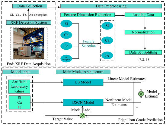
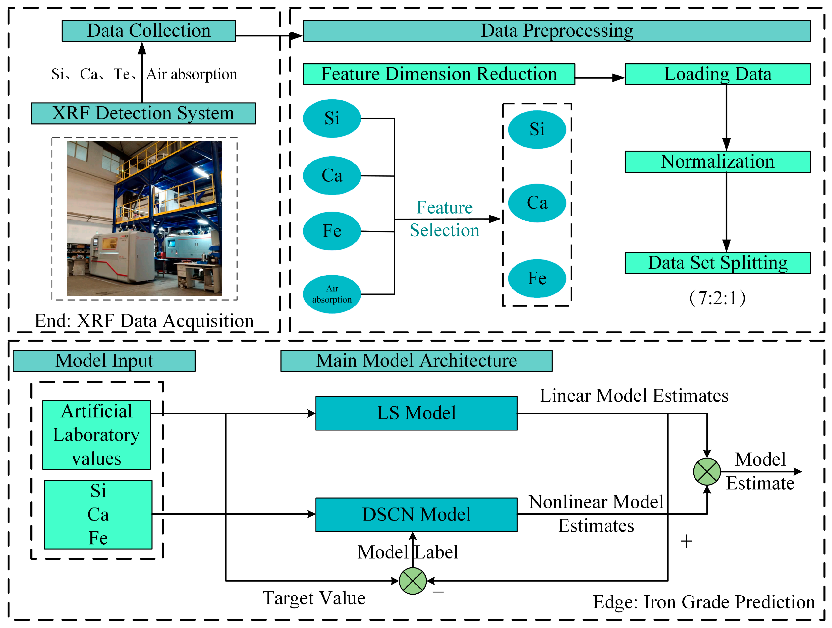
In order to improve the accuracy of detecting the grade of total iron ore under the influence of matrix effects, this paper divides the regression model into two parts: a preliminary grade estimation model and a correction compensation model. The preliminary grade estimation model is constructed based on the known portion derived from mechanism analysis, while the correction compensation model is a data-driven model. Use an XRF detection system to obtain the X-ray fluorescence intensity values of silicon, iron, calcium, silicon dioxide, and air absorption in the total iron ore sample, and preprocess them to obtain the dataset $D=\{x,y\}$, where $x$ denotes the XRF fluorescence intensity values of the measured elements and air absorption, obtained using an XRF spectrometer, and $y$ represents the true total iron grade of the elements to be measured, determined through manual laboratory assays performed on-site in the industrial environment; perform feature processing on dataset $D=\{x,y\}$ to select a robust feature set $S=\{x^{\ast },y\}$, where $x^{\ast }$ denotes the fluorescence intensity values of the main input features after selection; based on robust feature selection $S=\{x^{\ast },y\}$, a preliminary grade value estimation model was constructed using linear regression methods. The estimation results of this model are the preliminary grade values $y^{\ast }$ of the elements to be measured. Construct an interpolated label $\Delta y=\left|y^{*}-y\right|$ to replace the manual test value of $S=\{x^{\ast },y\}$ to obtain a new dataset $G=\{x^{\ast },\Delta y\}$. Based on $G=\{x^{\ast },\Delta y\}$, a correction compensation model is constructed using a dynamic regularization stochastic configuration networks. The estimated results of this model are the correction compensation values $\Delta y^{\ast }$ for the elements to be measured. The sum of the estimated results output from the preliminary grade prediction model and the correction compensation model is the final grade estimate $(y^{†}=y^{\ast }+\Delta y^{\ast })$. Figure 5 shows the structural diagram of the XRF-based iron ore grade detection method.

Figure 5. Structural diagram of XRF total iron ore grade detection method.

3.2. Feature Engineering Processing

In order to eliminate redundant information in high-dimensional input features and improve the generalization ability of the model, this paper introduces Lasso regression for feature selection. To further improve optimization efficiency and ensure convergence, the alternating direction method of multipliers is used to solve the Lasso problem. The experiment used a dataset $D=\{x,y\}$ collected from a real industrial site. The dataset $D=\{x,y\}$ was standardized to obtain the input feature matrix $A$.

The objective of Lasso regression is to minimize the linear regression loss with L1 regularization:

$$\underset{\vartheta }{\min }\left\{{\displaystyle \frac{1}{2}}{‖A\vartheta -\kappa ‖}_2^2+\tau {‖\vartheta ‖}_1\right\}$$

(8)

where $A\in {ℝ}^{m\times n}$ represents the input feature matrix (where $m$ is the number of samples and $n$ is the number of features); $\vartheta \in {ℝ}^n$ is the weight coefficient vector to be solved; $\kappa \in {ℝ}^m$ represents the output variable vector; $\tau$ represents the L1 regularization parameter, which is used to control the sparsity intensity (the larger $\tau$ is, the fewer features are selected).

The non-smoothness of Lasso regression originates from the ${‖\vartheta ‖}_1$ term, which is difficult to solve using traditional optimization methods. To address the non-smoothness caused by L1 regularization, this paper uses the alternating direction method of multipliers (ADMM) for optimization. ADMM is an efficient iterative method for constraint optimization problems with separable structures. Its core idea is to introduce auxiliary variables $z$ to transform the original non-separable non-smooth optimization objective into a separable problem with equality constraints, the conversion relationship is mathematically described by (9):

$$\underset{\vartheta ,z}{\min }\left\{{\displaystyle \frac{1}{2}}{‖A\vartheta -\kappa ‖}_2^2+\tau {‖z‖}_1\right\}$$

(9)

$$s.t.:\vartheta -z=0$$

(10)

Construct an augmented Lagrange function, introducing Lagrange multiplier $\psi \in {ℝ}^n$ and augmented term $\rho$:

$${\mathrm{\Gamma }}_p(\vartheta ,z,\psi )={\displaystyle \frac{1}{2}}{‖A\vartheta -\kappa ‖}_2^2+\tau {‖z‖}_1+{\psi }^T(x-z)+{\displaystyle \frac{\rho }{2}}{‖x-z‖}_2^2$$

(11)

Introducing the scaled dual variable $u={\displaystyle \frac{1}{\rho }}\psi$, then:

$$\psi =\rho u\Rightarrow {\psi }^T(x-z)=\rho u^T(x-z)$$

(12)

Substituting (12) into (11), we have:

$$\begin{array}{l}{\mathrm{\Gamma }}_{\rho }(\vartheta ,z,u)={\displaystyle \frac{1}{2}}{‖A\vartheta -\kappa ‖}_2^2+\tau {‖z‖}_1+\rho u^T(x-z)+{\displaystyle \frac{\rho }{2}}{‖x-z‖}_2^2\\ \Rightarrow {\displaystyle \frac{\rho }{2}}{‖x-z+u‖}_2^2={\displaystyle \frac{\rho }{2}}{‖x-z‖}_2^2+\rho u^T(x-z)+{\displaystyle \frac{\rho }{2}}{‖u‖}_2^2\\ \Rightarrow {\mathrm{\Gamma }}_{\rho }(\vartheta ,z,u)={\displaystyle \frac{1}{2}}{‖A\vartheta -\kappa ‖}_2^2+\tau {‖z‖}_1+{\displaystyle \frac{\rho }{2}}{‖x-z+u‖}_2^2-{\displaystyle \frac{\rho }{2}}{‖u‖}_2^2\end{array}$$

(13)

ADMM iteratively updates $\vartheta$, $z$ and $u$ in turn to ultimately find the optimal solution. The iterative steps are as follows:

(1)

Update subproblem $\vartheta$: fix $z^k$ and $u^k$, update ${\vartheta }^{k+1}$, and use the update equation shown in (14):

$${\vartheta }^{(k+1)}=\arg \underset{\vartheta }{\min \left\{{\displaystyle \frac{1}{2}}{‖A\vartheta -\kappa ‖}_2^2+{\displaystyle \frac{\rho }{2}}{‖\vartheta -z+u‖}_2^2\right\}}$$

(14)

$${\vartheta }^{(k+1)}={(A^{T}A+\rho I)}^{-1}(A^T\kappa +\rho (z^{(k)}-u^{(k)}))$$

(15)

where $I$ represents the unit matrix, with dimension $n\times n$; $z^{(k)}$ represents the auxiliary variable of the $k$th iteration; $u^{(k)}$ represents the Lagrange multiplier of the $k$th iteration.

(2)

Update subproblem $z$: fix $x^{k+1}$ and $u^k$, update $z^{k+1}$, and use the update equation shown in (16):

$$z^{(k+1)}=\arg \underset{z}{\min }\left\{\tau {‖z‖}_1+{\displaystyle \frac{\rho }{2}}{‖{\vartheta }^{(k+1)}-z+u^{(k)}‖}_2^2\right\}$$

(16)

$$z^{(k+1)}=S_{\lambda /\rho }({\vartheta }^{(k+1)}+u^{(k)})$$

(17)

$$S_{\lambda /\rho }(\theta )=sign(\theta )\cdot \max (\left|\theta \right|-{\displaystyle \frac{\lambda }{\rho }},0)$$

(18)

where $\theta$ represents the input vector ${\vartheta }^{(k+1)}+u^{(k)}$.

(3)

Update dual variables:

$$u^{(k+1)}=u^{(k)}+{\vartheta }^{(k+1)}-z^{(k+1)}$$

(19)

The iterative process of solving the three subproblems guarantees convergence, which is mathematically described by (20):

$$‖{\vartheta }^{(k+1)}-z^{(k+1)}‖\le \epsilon$$

(20)

where $\epsilon >0$ is the preset tolerance threshold. This condition ensures that ADMM stops iteration under the premise of satisfying constraint consistency, indicating that the algorithm has reached a convergent state.

3.3. Preliminary Grade Estimation Model Based on Least Squares

This paper investigates the stimulated X-ray fluorescence mechanism in total iron ore samples and develops a preliminary grade estimation model that quantifies the relationship between characteristic spectral line intensity and ore grade. To describe the linear relationship within this model, the LS regression algorithm [26,27] is employed to determine and optimize the unknown parameters.

Collect $N$ sample data as a training set through laboratory artificial testing methods and upper computer software platforms. The training dataset is represented by $S=\{x^{\ast },y\}$, $X^{\ast }={[x_1^{\ast },x_2^{*},\dots ,x_N^{*}]}^T\in R^{N\times 1}$ is the input data, represented by the X-ray fluorescence intensity values of the elements to be tested in $N$ samples, $Y={[y_1,y_2,\dots ,y_N]}^T\in R^{N\times 1}$ is the expected output of the linear term, represented by the artificial assay grades of the elements to be tested in $N$ samples. This paper hopes to use linear relationships:

$$y=k{x}^{*}+d$$

(21)

To describe the relationship between $y$ and $x^{*}$, where $k$ and $d$ are the regression coefficients to be estimated.

(1)

Optimization objectives

In order to find the optimal values of $k$ and $d$, the residual sum of squares (RSS) is introduced as the optimization objective function:

$$RSS={\displaystyle \sum _{i=1}^N{(y_i-(k{x}_i^{*}+d))}^2}$$

(22)

We need to minimize the objective function, find the values of $k$ and $d$ that minimize RSS.

(2)

Parameter estimation

By taking the partial derivatives of RSS with respect to $k$ and $d$ and setting them to zero, we have the following (23):

$$\left\{\begin{array}{c}{\displaystyle \frac{\partial RSS}{\partial k}}=-2{\displaystyle \sum _{i=1}^N(y_i-k{x}_i-d)x_i=0}\\ {\displaystyle \frac{\partial RSS}{\partial d}}=-2{\displaystyle \sum _{i=1}^N(y_i-k{x}_i-d)=0}\end{array}\right.$$

(23)

By rearranging (23), we have (24):

$$\left\{\begin{array}{c}{\displaystyle \sum _{i=1}^N{x}_i{y}_i-k{\displaystyle \sum _{i=1}^N{x}_i^2-d{\displaystyle \sum _{i=1}^N{x}_i=0}}}\\ {\displaystyle \sum _{i=1}^N{y}_i-k{\displaystyle \sum _{i=1}^N{x}_i-dN=0}}\end{array}\right.$$

(24)

Solving (24) yields optimal estimates of $k$ and $d$.

$$\left\{\begin{array}{c}k={\displaystyle \frac{N{\displaystyle \sum _{i=1}^N{x}_i{y}_i-{\displaystyle \sum _{i=1}^N{x}_i}}{\displaystyle \sum _{i=1}^N{y}_i}}{N{\displaystyle \sum _{i=1}^N{x}_i^2}-{({\displaystyle \sum _{i=1}^N{x}_i})}^2}}\\ d={\displaystyle \frac{{\displaystyle \sum _{i=1}^N{y}_i-k{\displaystyle \sum _{i=1}^N{x}_i}}}{N}}\end{array}\right.$$

(25)

3.4. Correction Compensation Model Based on Dynamic Regularization Stochastic Configuration Networks

The unknown nonlinear terms in this study are modeled using a correction compensation framework, with a dynamic regularization stochastic configuration networks (DSCN) as the core algorithm. Stochastic configuration networks (SCN) [28,29,30] are an incremental supervised learning approach that dynamically expands the hidden layer and computes output weights via least squares until a predefined accuracy or node limit is reached. However, traditional SCN employ fixed regularization, which cannot differentiate node importance, leading to overfitting and loss of effective information. These limitations are especially challenging in mineral X-ray fluorescence (XRF) detection, where noise and matrix effects from multiple interfering elements complicate analysis. To address this, a dynamic regularization mechanism is proposed that adaptively adjusts regularization based on node weight norms, enhancing sparsity for low-contribution nodes while relaxing constraints on important nodes, thereby balancing model complexity and generalization and ensuring robustness in noisy and complex environments.

3.4.1. Dynamic Regularization Stochastic Configuration Networks

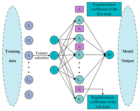
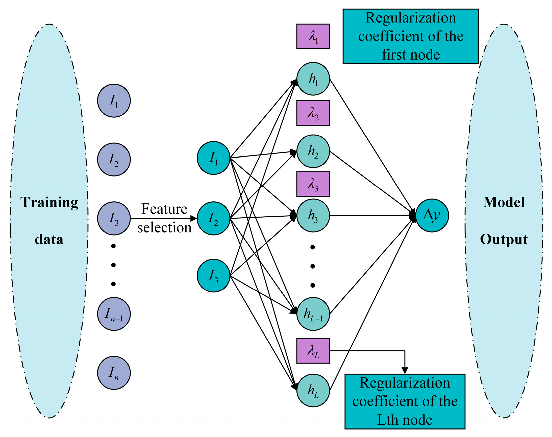
The estimation process of nonlinear terms in the correction compensation model using the DSCN is as follows: Based on robust feature selection $S=\{x^{\ast },y\}$, a preliminary grade value estimation model was constructed using linear regression methods. The estimation results of this model are the preliminary grade values $y^{\ast }$ of the elements to be measured. Construct an interpolated label $\Delta y=\left|y^{*}-y\right|$ to replace the manual test value of $S=\{x^{\ast },y\}$ to obtain a new dataset $G=\{x^{\ast },\Delta y\}$. Given the training set $\left\{\left.X^{\ast },\Delta Y\right\}\right.$, $X^{\ast }={(x_1^{*},\dots ,x_m^{*},\dots ,x_N^{*})}^T\in R^{N\times (n+1)}$ represents the input data, $x_m=(I_1,I_2,I_i,\dots ,I_n)\in R^{n+1}$, $m=1,2,\dots ,N$, $I_i$ represents the X-ray fluorescence intensity values of the elements to be tested, represents the X-ray fluorescence intensity values of $n$ coexisting elements; $\Delta Y={(y_1,\dots ,y_m,\dots ,y_N)}^T\in R^{N\times 1}$ represents the expected output of the nonlinear term. The neural network architecture diagram is shown in Figure 6.

Figure 6. DSCN Network.

(1)

Given an $span(\mathrm{\Gamma })$, which represents the function space composed of $\mathrm{\Gamma }$. Assume that $span(\mathrm{\Gamma })$ is dense in space $L_2$, and $\forall g\in \mathrm{\Gamma },0<‖g‖<b_g$, where $b_g\in R^{+}$. For a given positive real number ${\Lambda }_L$, there exists a sufficiently small positive real number $\epsilon ({\Lambda }_L)$. Given $1-\epsilon <r<1$, a non-negative real number sequence $u_L$ satisfies $1-\epsilon -r<u_L<(1-r)$. Given the objective function $f=[\begin{array}{cccc}{f}_1& f_2& \dots & f_m\end{array}]:R^d\to R^m$, where $d$ and $m$ represent the dimensions of the input samples and the model output, Assuming that a DSCN with $L-1$ hidden layer nodes has been constructed, its output $f_{L-1}$ can be expressed as:

$$f_{L-1}^T(X^{*})={\displaystyle \sum _{j=1}^{L-1}{\beta }_j}{g}_j({\omega }_j^T{X}^{{*}^T}+b_j)$$

(26)

where ${\beta }_j$ represents the output weight of hidden node $j$; $g_j(\cdot )$ represents the $j$th activation function; ${\omega }_j$ and $b_j$ represent the input weight and bias of the $j$th hidden node in the hidden layer, respectively. Among them, ${\omega }_j$ and $b_j$ are randomly assigned within the adjustable intervals ${\left[-\eta ,\eta \right]}^d$ and $\left[-\eta ,\eta \right]$, and $\eta$ is automatically assigned from the interval $\left[{\eta }_{\min },\Delta \eta ,{\eta }_{\max }\right]$.

(2)

Calculate the output residuals with $L-1$ hidden layer nodes:

$$e_{L-1}=f-f_{L-1}(X^{*})$$

(27)

(3)

The DSCN introduces a new hidden layer node via a supervisory mechanism, with the corresponding formulation expressed in (28):

$$\left\{\begin{array}{c}{\xi }_L={\displaystyle \sum _{q=1}^m{\xi }_{L,q}\ge 0,{\xi }_{L,q}=\frac{{\left(e_{L-1,q}^T{h}_L\right)}^2}{\gamma }-\left(1-r-{\mu }_L\right)e_{L-1,q}^T{e}_{L-1,q},q=1,2,\dots ,m}\\ h_L=\left[g_L\left({\omega }_L^T{x}_1^{*}+b_L\right),g_L\left({\omega }_L^T{x}_2^{*}+b_L\right),\right.\dots ,{\left.g_L\left({\omega }_L^T{x}_N^{*}+b_L\right)\right]}^T\end{array}\right.$$

(28)

where $\gamma ={(h_L^T\cdot h_L+{\Lambda }_L)}^2/(h_L^T\cdot h_L+2{\Lambda }_L)$ is given, $1-\epsilon <r<1$ is set, and ${\mu }_L=(1-r)/(L+1)$ is defined, ${\Lambda }_L$ are the regularization coefficients of the $L$-th node. Randomly configure $T_{\max }$ times, each time randomly selecting the input weights ${\omega }_L$ and biases $b_L$ of the $L$-th hidden layer node within a certain range, and calculating ${\xi }_{L,q},q=1,2,\dots ,m$. If $\min \{{\xi }_{L,1},{\xi }_{L,2},\dots ,{\xi }_{L,q}\}\ge 0$, store ${\omega }_L$, $b_L$ and ${\xi }_{L,q}$; if all ${\xi }_{L,q}$ do not meet the conditions, select a larger $r$ value to reconfigure. After random configuration is complete, select the largest ${\displaystyle {\sum }_{q=1}^m{\xi }_{L,q}}$ corresponding to ${\omega }_L$ and $b_L$ as the input weights and biases of the $L$-th node.

(4)

The output weights of the DSCN network with $L$ nodes can be obtained by solving the DSCN objective function, which is expressed as (29):

$$\beta =\arg \underset{\beta }{\min }\left({‖H_L\beta -f‖}^2+{\displaystyle \sum _{l=1}^L{\lambda }_l{\beta }_l^2}\right)$$

(29)

where $H_L$ is the hidden layer output matrix, $\beta =[{\beta }_1,{\beta }_2,\dots ,{\beta }_L]$ is the output weight vector, ${\lambda }_l$ is the dynamic regularization coefficient, and $L$ is the number of nodes. In DSCN, the update method for dynamic regularization is expressed as (33):

$${\lambda }_l={\displaystyle \frac{c}{{‖{\beta }_{l-1}‖}_2+\varsigma }}$$

(30)

where $c$ is the global regularization parameter; $\varsigma$ is a very small number to prevent division by zero in the denominator; ${‖{\beta }_{l-1}‖}_2$ is the L2 norm of the weight of the $l-1$th node.

(5)

Solve for the output weights using (28) and (29):

$$\beta ={(H_L^T{H}_L+\Lambda )}^{-1}{H}_L^T\Delta Y$$

(31)

where $\Lambda =\left[\begin{array}{ccc}{\lambda }_1& & \\ & \ddots & \\ & & {\lambda }_L\end{array}\right]$ is a diagonal matrix.

(6)

Obtain the estimated value of the total iron ore grade correction compensation model, expressed as:

$$\Delta y={\displaystyle \sum _{j=1}^L{\beta }_j}{g}_j\left({\omega }_j^T{X}^{*}+b_j\right)$$

(32)

3.4.2. Convergence Analysis and Proof of the DSCN

Assume that $span(\mathrm{\Gamma })$ is dense in space $L_2$, and $\forall g\in \mathrm{\Gamma },0<‖g‖<b_g$, where $b_g\in R^{+}$. For a given positive real number ${\Lambda }_L$, there exists a sufficiently small positive real number $\epsilon ({\Lambda }_L)$. Given $1-\epsilon <r<1$, a non-negative real number sequence $u_L$ satisfies $1-\epsilon -r<u_L<(1-r)$. For $L=1,2,\dots$ and $q=1,2,\dots ,m$, the following definitions are made:

$${\delta }_L^{*}={\displaystyle \sum _{q=1}^m{\delta }_{L,q}^{*}},{\delta }_{L,q}^{*}=(1-r-u_L){‖e_{L-1,q}^{*}‖}^2$$

(33)

$$\xi =\underset{L\to \infty }{\lim }{(1-\epsilon )}^L<1$$

(34)

$$\gamma =\underset{L\to \infty }{\lim }{\displaystyle \prod _{k=1}^L(r+u_k)<1}$$

(35)

If the generated random basis function $g_L$ satisfies (36):

$${⟨e_{L-1},g_L⟩}^2\ge {\displaystyle \frac{{(h_L^T\cdot h_L+{\Lambda }_L)}^2}{(h_L^T\cdot h_L+2{\Lambda }_L)}}{\delta }_{L,q}^{*}$$

(36)

The output weight ${\beta }_{L,q}$ is calculated according to (37):

$$[{\beta }_1^{*},{\beta }_2^{*},\dots ,{\beta }_L^{*}]=\underset{\beta }{\arg \min }{\displaystyle \frac{1}{2{\Lambda }_L}}{‖f-{\displaystyle \sum _{j=1}^L{\beta }_j{g}_j}‖}^2+{\displaystyle \frac{1}{2}}{‖\beta ‖}_2^2$$

(37)

So, $\sqrt{\xi }‖f‖\le \underset{L\to +\infty }{\lim }‖f-f_L^{*}‖\le \sqrt{\gamma }‖f‖$, where $f_L^{*}={\displaystyle \sum _{j=1}^L{\beta }_j^{*}}{g}_j$, ${\beta }_j^{*}={[{\beta }_{j,1}^{*},{\beta }_{j,2}^{*},\dots ,{\beta }_{j,m}^{*}]}^T$.

Proof. 

where $e_L^{*}=f-{\displaystyle \sum _{j=1}^L{\beta }_j^{*}}{g}_j=[e_{L,1}^{*},e_{L,2}^{*},\dots ,e_{L,m}^{*}]$, define intermediate variables ${\tilde{\beta }}_{L,q}=⟨e_{L-1,q}^{*},g_L⟩/\left(\Vert g_L{\Vert }^2+{\Lambda }_L\right)$, $\widetilde{e_L}=e_{L-1}^{*}-{\tilde{\beta }}_L{g}_L$, where $\stackrel{\sim }{{\beta }_L}={[{\beta }_{L,1},{\beta }_{L,2},\dots ,{\beta }_{L,m}]}^T$, $e_0^{*}=f$.□

It is easy to see that ${‖e_L^{*}‖}^2\le {‖\widetilde{e_L}‖}^2=\Vert e_{L-1}^{*}-{‖e_{L-1}^{*}‖}^2\le {‖\widetilde{e_{L-1}}‖}^2$, so we have:

$$\begin{array}{l}{‖e_L^{*}‖}^2-{‖e_{L-1}^{*}‖}^2\le {‖\widetilde{e_L}‖}^2-{‖e_{L-1}^{*}‖}^2\\ ={\displaystyle \sum _{q=1}^m(⟨}{e}_{L-1,q}^{*}-{\tilde{\beta }}_{L,q}{g}_L,e_{L-1,q}^{*}-{\tilde{\beta }}_{L,q}{g}_L⟩-⟨e_{L-1,q}^{*},e_{L-1,q}^{*}⟩)\\ ={\displaystyle \sum _{q=1}^m(-2⟨}{e}_{L-1,q}^{*},{\tilde{\beta }}_{L,q}{g}_L⟩+⟨{\tilde{\beta }}_{L,q}{g}_L,{\tilde{\beta }}_{L,q}{g}_L⟩)\\ ={\displaystyle \sum _{q=1}^m\left(\frac{-2{⟨e_{L-1,q}^{*},g_L⟩}^2}{{‖g_L‖}^2+{\Lambda }_L}+\frac{{⟨e_{L-1,q}^{*},g_L⟩}^2{‖g_L‖}^2}{{\left({‖g_L‖}^2+2{\Lambda }_L\right)}^2}\right)}\\ =-{\displaystyle \frac{{\displaystyle \sum _{q=1}^m{⟨e_{L-1,q}^{*},g_L⟩}^2}}{{\left({‖g_L‖}^2+{\Lambda }_L\right)}^2/\left({‖g_L‖}^2+2{\Lambda }_L\right)}}\end{array}$$

(38)

Since the $L_2$-norm produces biased estimates, there exists a sufficiently small positive real number $\theta$ such that ${‖e_L^{*}‖}^2>\theta$ holds. Then we obtain:

$${‖e_{L-1}^{*}‖}^2-{‖e_L^{*}‖}^2\le {‖e_{L-1}^{*}‖}^2-\theta$$

(39)

Let ${‖e_{L-1}^{*}‖}^2-\theta =\epsilon {‖e_{L-1}^{*}‖}^2$ and $0<\epsilon <1$. Using (39), we have:

$$(1-\epsilon ){‖e_{L-1}^{*}‖}^2\le {‖e_L^{*}‖}^2$$

(40)

From (29), (33) and (35), we have:

$$\begin{array}{l}{‖e_L^{*}‖}^2-(r+u_L){‖e_{L-1}^{*}‖}^2\le {‖\widetilde{e_L}‖}^2-(r+u_L){‖e_{L-1}^{*}‖}^2\\ ={\displaystyle \sum _{q=1}^m(⟨}{e}_{L-1,q}^{*}-{\tilde{\beta }}_{L,q}{g}_L,e_{L-1,q}^{*}-{\tilde{\beta }}_{L,q}{g}_L⟩-(r+u_L)⟨e_{L-1,q}^{*},e_{L-1,q}^{*}⟩)\\ ={\displaystyle \sum _{q=1}^m((}(1-r-u_L)⟨e_{L-1,q}^{*},e_{L-1,q}^{*}⟩-2⟨e_{L-1,q}^{*},{\tilde{\beta }}_{L,q}{g}_L⟩+⟨{\tilde{\beta }}_{L,q}{g}_L,{\tilde{\beta }}_{L,q}{g}_L⟩)\\ =(1-r-u_L){‖e_{L-1}^{*}‖}^2+{\displaystyle \sum _{q=1}^m\left(\frac{-2{⟨e_{L-1,q}^{*},g_L⟩}^2}{{‖g_L‖}^2+{\Lambda }_L}+\frac{{⟨e_{L-1,q}^{*},g_L⟩}^2{‖g_L‖}^2}{{\left({‖g_L‖}^2+2{\Lambda }_L\right)}^2}\right)}\\ =(1-r-u_L){‖e_{L-1}^{*}‖}^2-{\displaystyle \frac{{\displaystyle \sum _{q=1}^m{⟨e_{L-1,q}^{*},g_L⟩}^2}}{{\left({‖g_L‖}^2+{\Lambda }_L\right)}^2/\left({‖g_L‖}^2+2{\Lambda }_L\right)}}\\ \le {\delta }_L-{\displaystyle \frac{{\displaystyle \sum _{q=1}^m{⟨e_{L-1,q}^{*},g_L⟩}^2}}{{\left(b_g^2+{\Lambda }_L\right)}^2/\left(b_g^2+2{\Lambda }_L\right)}}\le 0\end{array}$$

(41)

The conclusion can be derived: $\sqrt{\xi }‖f‖\le \underset{L\to \infty }{\lim }‖e_L^{*}‖\le \sqrt{\gamma }‖f‖$.

3.4.3. Pseudocode Flow of the DSCN

Table 1 presents the pseudocode corresponding to the flow of the DSCN. Given training sample $\left(X,Y\right)$, where input data is $X=[x_1,x_2,\dots ,x_N]$ and output data is $Y=[y_1,y_2,\dots ,y_N]$; maximum number of hidden layer nodes is $L_{max}$= 100, $\epsilon$= 0.001 is the desired tolerance, maximum number of random configurations is $T_{max}$= 100; select a set of positive scalars $\gamma =\{{\varphi }_{min}:\Delta \varphi :{\varphi }_{max}\}$.

Table 1. Pseudocode flow of the DSCN.

Neural Network Training Phase: Random Parameter Configuration and Output Weight Calculation
While $L\le L_{max}$ AND $\Vert e_0{\Vert }_F>\epsilon$, Do
1. Random parameter configuration
(1)	For $\lambda \in \gamma$,
(2)	For $k=1,2,\dots ,T_{max}$,
(3)	Randomly select $w_L$ and $b_L$ from ${[-\varphi ,\varphi ]}^d$ and $[-\varphi ,\varphi ]$, respectively;
(4)	Obtain $h_L$ and ${\xi }_{L,q}$ from Equation (28) and set $u_L=\left(1-r\right)/\left(L+1\right)$;
(5)	If $min{\xi }_{L,1},{\xi }_{L,2},\dots ,{\xi }_{L,m}\ge 0$
(6)	Store $w_L$ and $b_L$ in $W$, and ${\xi }_L={\displaystyle \sum _{q=1}^m{\xi }_{L,q}}$ in $\mathrm{\Omega }$;
(7)	Else return (2)
(8)	End If
(9)	End For
(10)	If $W$ is not an empty set
(11)	Find the maximum $w_L^{*}$ and $b_L^{*}$ corresponding to ${\xi }_L$ in $\mathrm{\Omega }$, and let $H_L=[h_1^{*},h_2^{*},\dots ,h_L^{*}]$;
(12)	Break (return 16);
(13)	Else generate $\tau$ randomly in $\tau \in (0,1-r)$, update $r:=r+\tau$, and return (2);
(14)	End If
(15)	End For
2. Update output weights
(16)	Obtain $H_L=[h_1^{*},h_2^{*},\dots ,h_L^{*}]$;
(17)	Update the global regularization coefficient: ${\lambda }_l={\displaystyle \frac{c}{{‖{\beta }_{l-1}^{*}‖}_2+\varsigma }}$;
(18)	Calculate output weights: ${\beta }^{*}=\left[\begin{array}{cccc}{\beta }_1^{*}& {\beta }_2^{*}& \dots & {\beta }_L^{*}\end{array}\right]$;
(19)	Calculate $e_L=Y-H_L{\beta }^{*}$;
(20)	let $e_0:=e_L$, $L:=L+1$;
End While
Return $\begin{array}{ccc}{\beta }_1^{*}& \dots & {\beta }_L^{*}\end{array}$, $w^{*}=\left[\begin{array}{cccc}{w}_1^{*}& w_2^{*}& \dots & w_L^{*}\end{array}\right]$, $b^{*}=\left[\begin{array}{cccc}{b}_1^{*}& b_2^{*}& \dots & b_L^{*}\end{array}\right]$

Neural network initialization: Let $e_0:={[t_1,t_2,\dots ,t_N]}^T$, given regularization matrix $\Lambda =\left[\begin{array}{ccc}{\lambda }_1& \dots & {\lambda }_L\end{array}\right]$, initialize regularization coefficient: ${\lambda }_1=0.0009$, ${\left[\begin{array}{cccc}{\lambda }_2& {\lambda }_3& \dots & {\lambda }_L\end{array}\right]}^{1\times (L-1)}=$ ${\left[\begin{array}{cccc}0& 0& \dots & 0\end{array}\right]}^{1\times (L-1)}$ a sufficiently small positive real number $\mathrm{\Psi }$, given $1-\mathrm{\Psi }<r<1$, $\mathrm{\Omega }$ and $W$ as two empty sets.

4. Experimental Analysis and Field Industrial Applications

4.1. Experimental Analysis

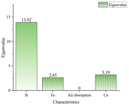
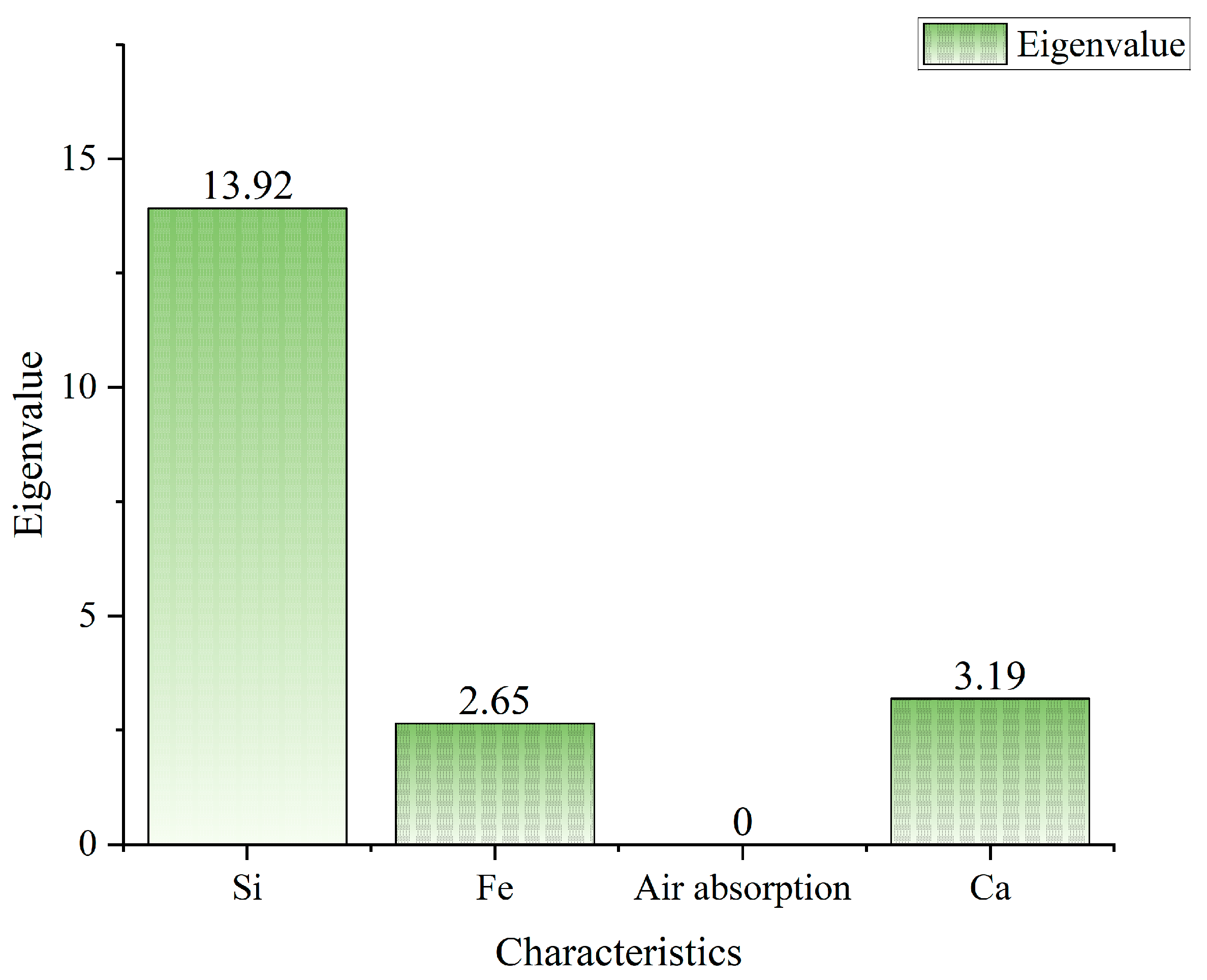
This study uses a dataset of total iron ore samples collected from industrial sites, where iron is the main element for measurement. X-ray fluorescence spectroscopy (XRF) analysis identified four matrix components—silicon (Si), calcium (Ca), iron (Fe), and air absorption—as possible interferences. In mineral samples, the characteristic X-ray emitted by Fe (Kα line, ~6.40 keV) can be partially absorbed by Si and Ca. Although Si has a lower atomic number, its absorption effect becomes significant when its content is high or the sample thickness is considerable. Ca, with a higher atomic number, exhibits much stronger absorption of the Fe Kα line. This strong absorption can substantially reduce the measured Fe fluorescence intensity and represents a major source of interference. Feature selection algorithms were used to identify Si, Ca, and Fe as the most important features for this study, based on their relevance to measuring the target element. Figure 7 shows the results of the feature selection.

Figure 7. Feature selection results.

The dataset consists of 153 datasets, which are divided into training sets and test sets at a ratio of 7:3. The dataset consists of 153 datasets, which are divided into training sets and test sets at a ratio of 7:3. The iron ore type is magnetite, and the XRF sensor operating parameters are a tube voltage of 12 kV, a tube current of 15 μA, and a sample detection cycle of 35 s. The grade of the first-stage magnetic separation product is 35%–40%, and that of the second-stage product is 55%–65%, with a model measurement accuracy of ≥95%. The sampling procedure is as follows: slurry samples are collected from the plant pipeline and pumped into the main system, with intermittent sampling performed by the sampler. The slurry is then sent to the pulping device, where its concentration is adjusted according to pressure feedback before being fed into the main system. The particle size of the first-stage magnetic separation product is approximately −200 mesh 40%–50%, and that of the second-stage product is approximately −200 mesh 70%–80%; these particle size characteristics are considered during pulping and feeding to ensure representative sampling and accurate analysis. After entering the main system, the slurry undergoes positive-pressure filtration to form filter cakes, which are subsequently crushed, stirred, and dried a second time to produce smooth and dense filter cakes. Finally, a robotic arm grabs the samples and delivers them to the detection chamber for analysis. To avoid the impact of inconsistent dimensions between features, this paper uses the maximum-minimum normalization method to process the data, linearly mapping each feature value to the [0, 1] interval. Order $X=[I_{Fe},I_{Ca},I_{Si}]$; $X$ is a $153\times 3$ order matrix, where $I_{(\cdot )}$ represents the X-ray fluorescence intensity values of element. Data processing is performed using (42):

$$X^{\ast }={\displaystyle \frac{X-\min (X)}{\max (X)-\min (X)}}$$

(42)

To validate the feasibility of the algorithm proposed in this paper, a comparison was conducted between the preliminary grade estimation model, the correction and compensation model, and the detection method combining preliminary grade estimation with correction and compensation. The preliminary grade estimation model is a linear model (Linear); the correction compensation model includes the SCN model; the detection method combining preliminary grade estimation with correction compensation includes the linear model combined with the SCN model (L-SCN model) and the linear model combined with the DSCN model (L-DSCN model). In this paper, the L-DSCN method uses cross-validation and grid search hyperparameter tuning techniques to select parameters such as the desired accuracy $\epsilon$, the maximum number of random configurations $T_{\max }$, and the dynamic regularization coefficient $\lambda$. To avoid selection bias influencing experimental results, hyperparameters of other models are determined through the same method.

This paper uses mean absolute error (MAE), root mean square error (RMSE), and coefficient of determination (R-Square, R²) as model evaluation indicators. The equations for calculating MAE, RMSE, and R² are as follows:

$$\mathrm{MAE}={\displaystyle \frac{1}{N}}{\displaystyle {\sum }_{i=1}^N\left|y_i-y_i^{†}\right|}$$

(43)

$$RMSE={\left({\displaystyle \frac{1}{N}}{\displaystyle \sum _{i=1}^N{(y_i-y_i^{†})}^2}\right)}^{{\displaystyle \frac{1}{2}}}$$

(44)

$$R^2=1-{\displaystyle \frac{{\displaystyle \sum _{i=1}^N{(y_i-y_i^{†})}^2}}{{\displaystyle \sum _{i=1}^N{(y_i-y_m)}^2}}}$$

(45)

where $N$ represents the number of samples, $y_i$ represents the grade value of the element to be tested in the test set, $y_i^{†}$ represents the predicted grade value of the element to be tested by the network model, and $y_m$ represents the average value of the artificial test value of the element to be tested.

Table 2 presents the quantitative evaluation metrics for the prediction of total iron ore grade using models established by four algorithms. As shown in the table, the L-DSCN model proposed in this paper achieves the lowest average absolute error (0.3092) and root mean square error (0.5561) among the four algorithms. The coefficient of determination (R²) reaches 99.91%, which is very close to the ideal value of 1. All evaluation metrics listed in the table exhibit superior performance compared to the other four algorithms, demonstrating that the L-DSCN intelligent detection model for total iron ore grade proposed in this study exhibits exceptional accuracy and robustness. For clarity, the classical linear method used as the reference baseline in this comparison is the least squares (LS) algorithm. For the Transformer model used in comparison, the basic parameter settings were max Epochs = 50, mini Batch Size = 16, and learning Rate = 0.001.

Table 2. The accuracy rate of different algorithms.

Model	MAE	RMSE	R2%
Linear (LS)	3.7771	1.9434	98.94%
SCN	3.0193	1.7376	99.15%
Transformer	1.2329	1.4358	99.49%
L-SCN	1.1404	1.0679	99.45%
L-DSCN	0.3092	0.5561	99.91%

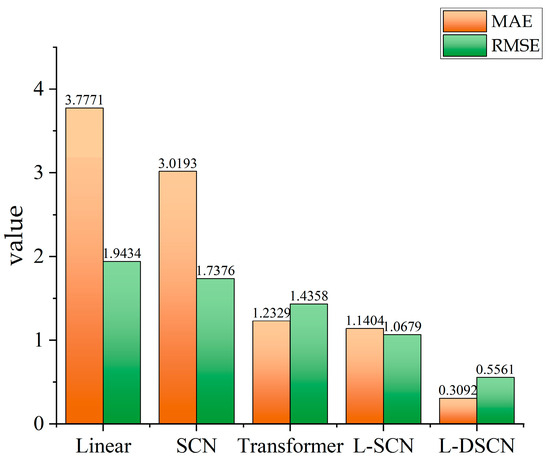
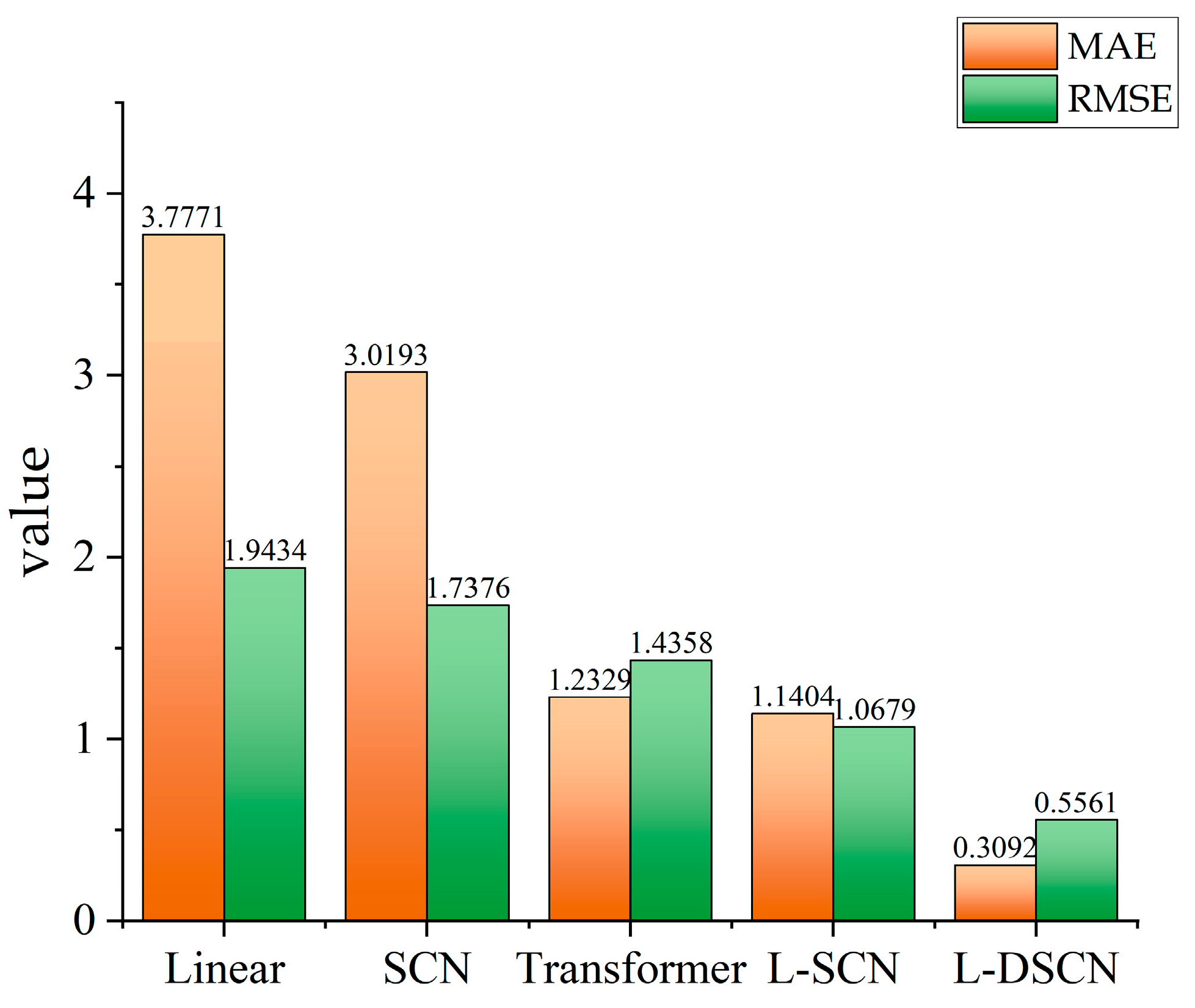
Figure 8 presents a comparison of RMSE and MAE for different models, including Linear, SCN, L-SCN, L-DSCN, and a Transformer-based deep learning model recently adopted in XRF-related research. As shown in the figure, the proposed L-DSCN achieves the lowest RMSE and MAE among all models, followed by L-SCN, while the Transformer model performs better than both the traditional Linear and SCN models. This result indicates that although Transformer-based frameworks can effectively capture complex nonlinear relationships in spectral data, their performance is still limited by their high computational cost and sensitivity to small-sample conditions commonly encountered in industrial XRF applications. In contrast, the L-DSCN architecture dynamically regularizes network nodes and integrates a linear estimation stage, enabling more stable convergence and higher prediction accuracy under complex matrix effects. Therefore, the proposed hybrid L-DSCN model not only surpasses traditional machine learning and baseline SCN methods but also demonstrates competitive advantages over modern deep learning frameworks in terms of accuracy, robustness, and computational efficiency, effectively meeting the industrial requirements for real-time total iron ore grade detection.

Figure 8. Comparison of RMSE and MAE for different models.

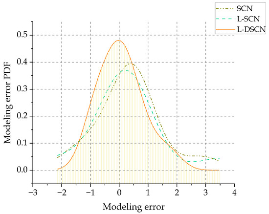
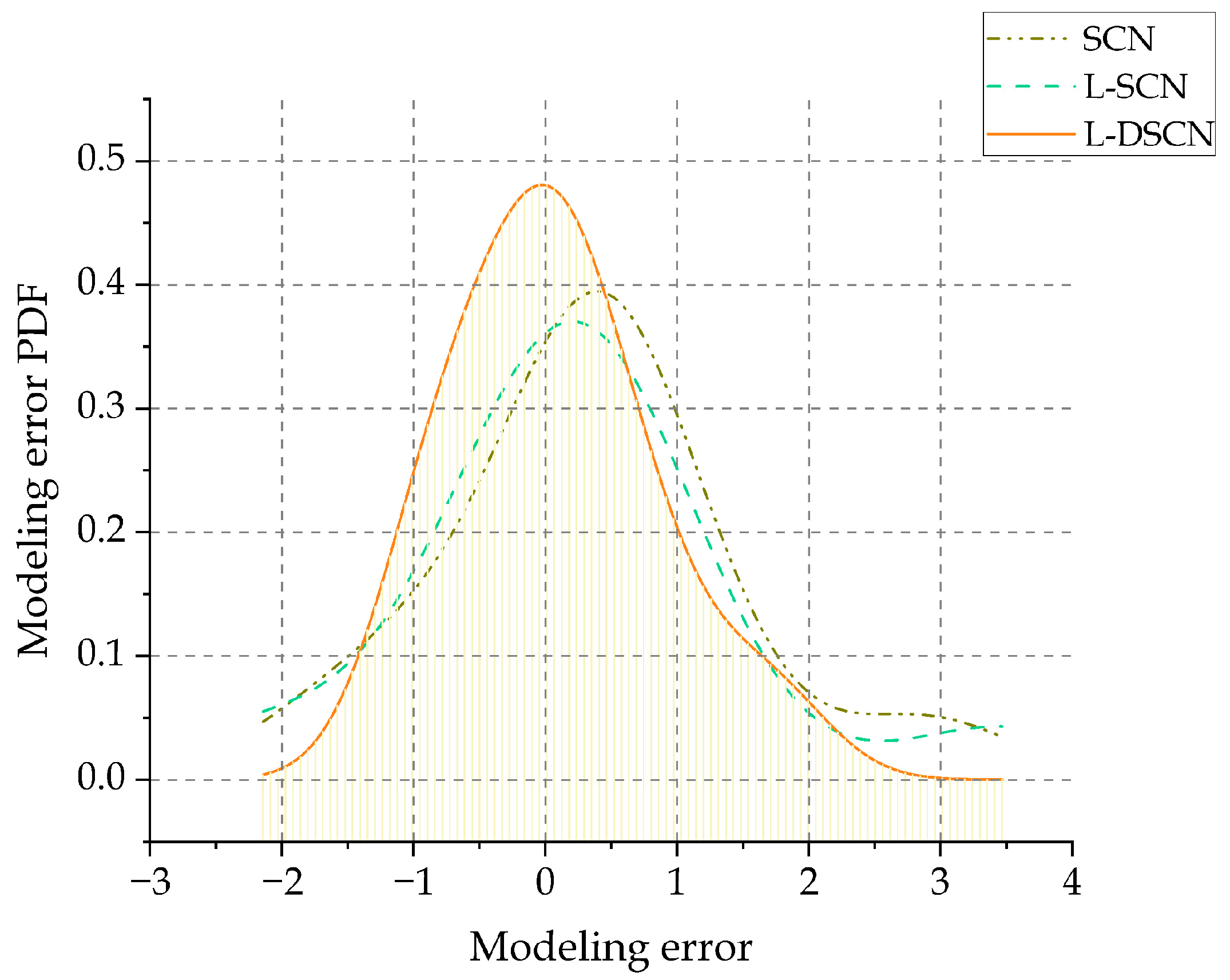
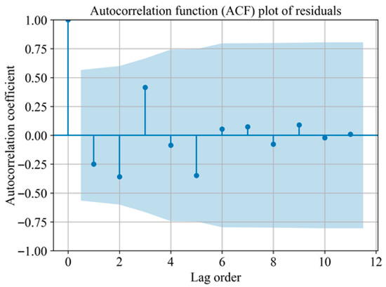
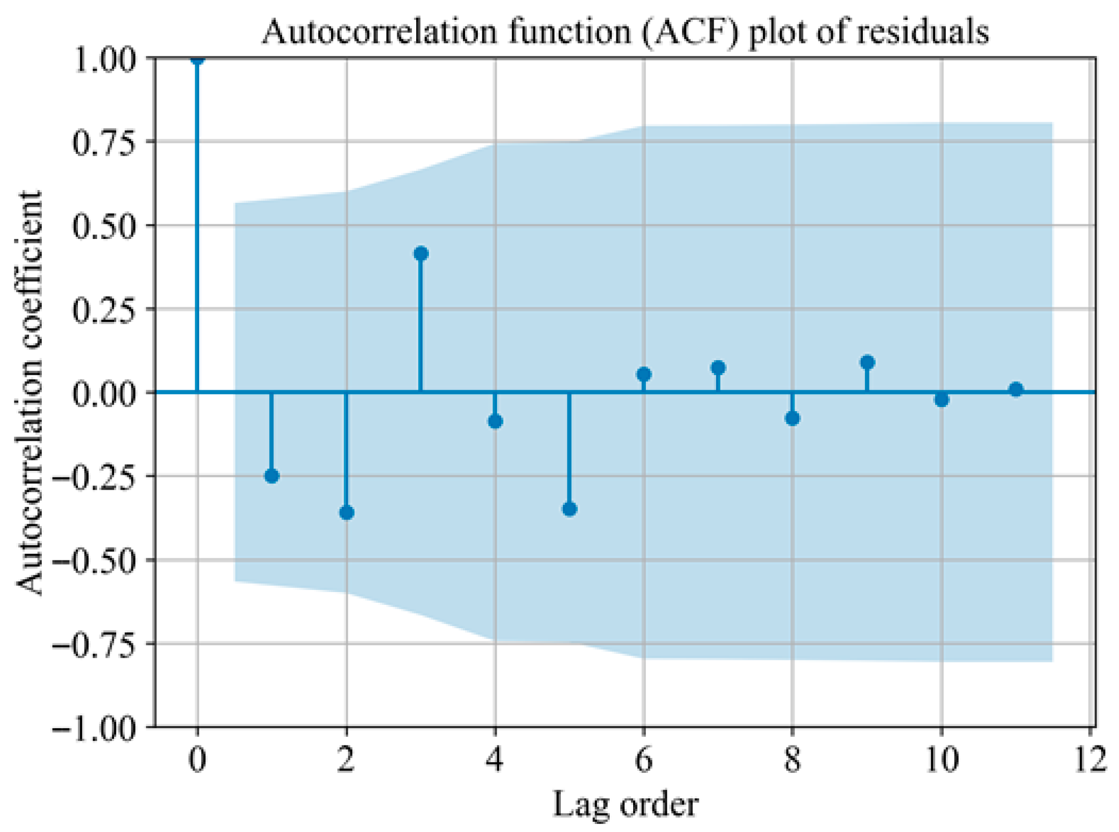
Figure 9 illustrates the probability density functions (PDFs) of estimation errors for the four models described in this study. The PDF curve of the L-DSCN model follows an approximately normal distribution, with low values at the tails and a peak at the center, indicating a high concentration of errors around the mean. This characteristic demonstrates excellent predictive accuracy and stability. Such a property makes the L-DSCN model more suitable for complex industrial production environments, whereas the other three models exhibit inferior performance. Furthermore, excluding the zero lag (where the autocorrelation function (ACF) value is 1), the ACF values for other lags are close to zero, indicating that the error sequence lacks significant autocorrelation (as shown in Figure 10). This aligns with white noise characteristics, suggesting that the model’s estimation errors are random and exhibit minimal correlation with the model itself. As a result, the L-DSCN model demonstrates superior estimation performance and strong generalization capabilities. This feature further improves its usefulness in complex industrial scenarios, while the other three models might perform worse under certain operating conditions.

Figure 9. Probability density function of estimation errors for different models.

Figure 10. Autocorrelation function of L-DSCN model residuals.

4.2. On-Site Industrial Applications

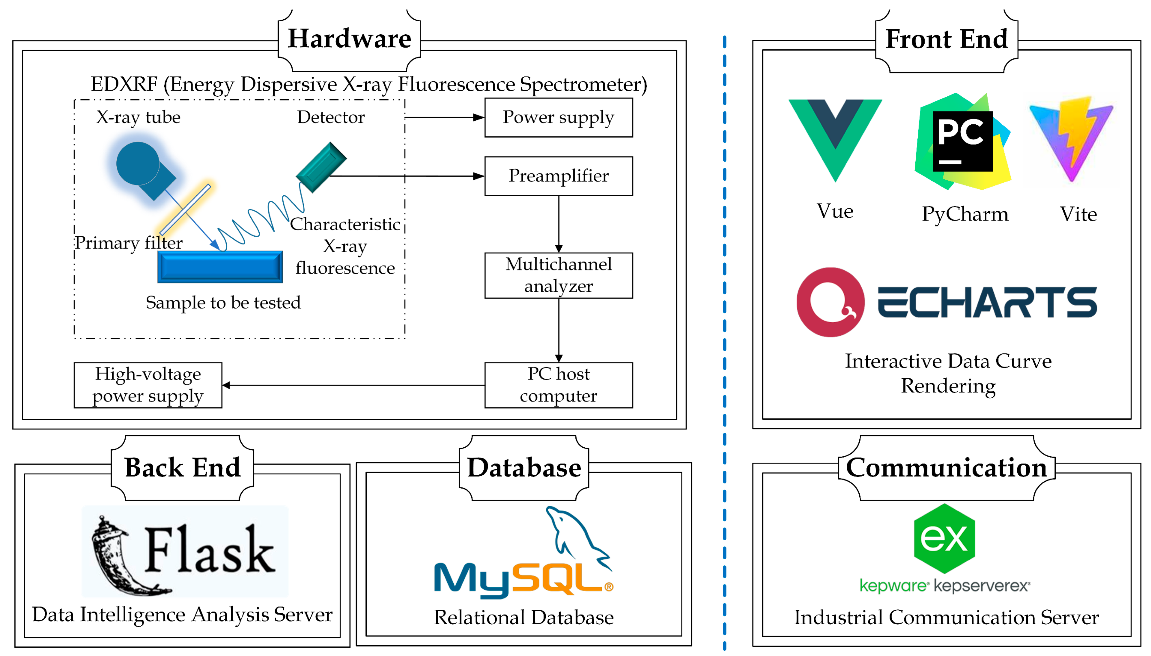
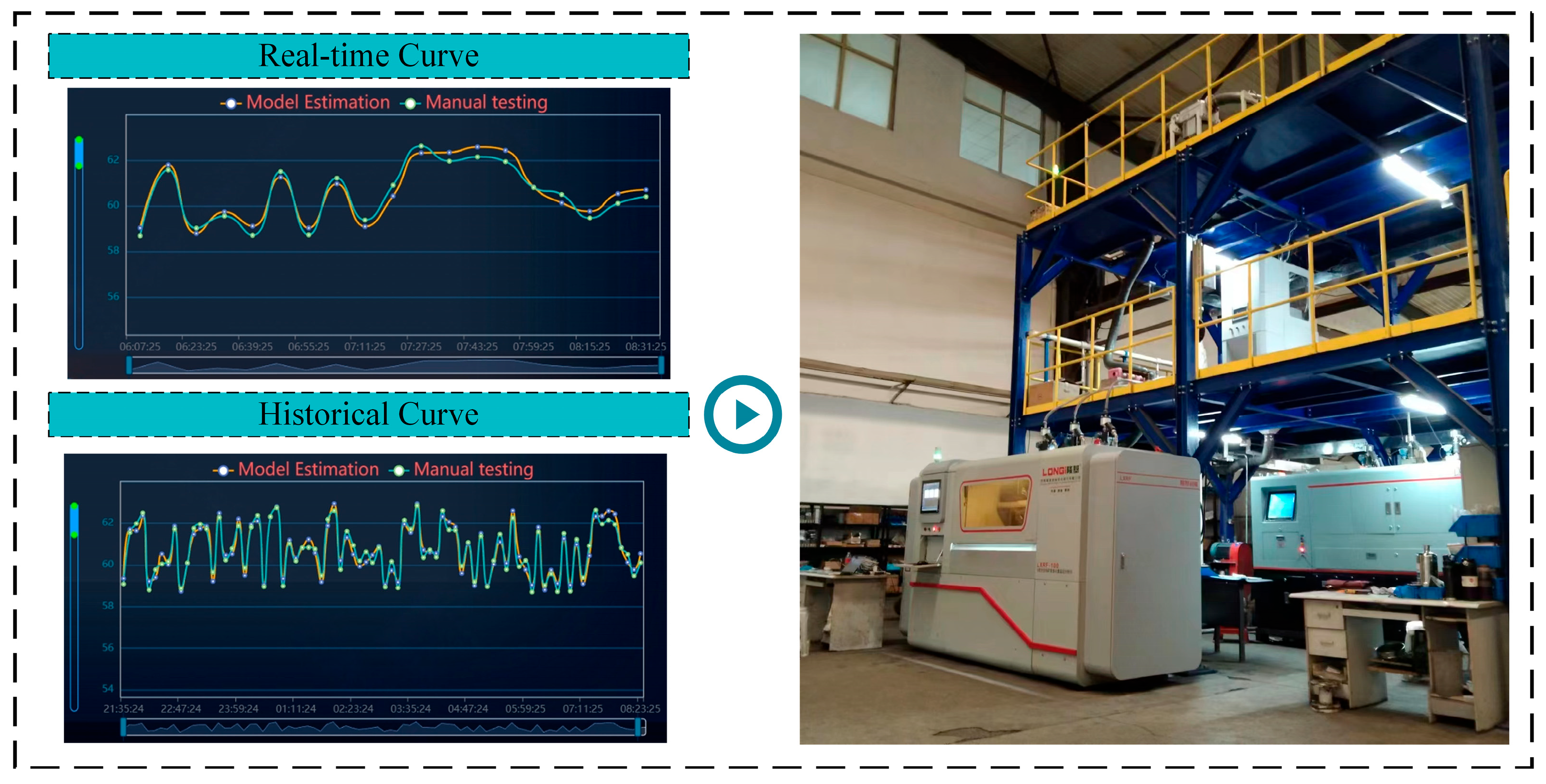
In industrial applications, maximizing the application of AI-driven data modeling technologies to unlock data value [31] is a key research direction in the field of intelligent detection of total iron ore grade values. To enable real-time detection of total iron ore grade values and provide a visual interface, this paper proposes a B/S architecture-based intelligent detection system for total iron ore grade values. The system’s software and hardware architecture is illustrated in Figure 11. This system adopts a front-end and back-end separation development approach. The front-end is developed using the Vue framework to handle interface interactions, while the back-end utilizes the Python 3.10 technology stack for business logic development. The front-end and back-end facilitate efficient collaboration through API interfaces. The back-end system maps the data model to database tables and integrates the method proposed in this paper to achieve core functionalities. Additionally, the system provides data storage, local area network access, data query, and export of data in Excel format, fulfilling the data processing and interaction requirements of practical applications. This intelligent detection system has been deployed at a mineral processing plant for over six months. Figure 12 illustrates the real-time curves of model grade estimates and manual laboratory measurements, as well as historical curves since the system’s deployment, along with the on-site installation effects. During this six-month deployment, manual laboratory assays were conducted 15–30 times per month to compare with the model’s predictions. The results show that the DSCN–LS model consistently met the production requirements in terms of both mean absolute error (MAE) and maximum absolute error, demonstrating stable and reliable performance across different operational conditions. When the model’s prediction accuracy drops below 95%, on-site personnel retrain the model using the latest production data to obtain optimal parameters, ensuring continuous improvement of detection accuracy. This demonstrates that, after a period of system operation and application, the intelligent detection method for total iron ore grade values proposed in this paper—based on DSCN and least squares—has achieved satisfactory results in industrial applications, with detection accuracy meeting the production process requirements for total iron ore grade value detection.

Figure 11. System hardware and software framework diagram.

Figure 12. Estimation of Total Iron Ore Grade and On-Site Installation Configuration.

5. Conclusions

This study presents a comprehensive quantitative analysis based on X-ray fluorescence spectroscopy (XRF), providing theoretical support for incorporating both target elements and interfering elements as model inputs. A robust framework for total iron ore grade detection was developed by integrating a preliminary grade estimation model with a correction compensation model, in which the preliminary model parameters are determined using the least squares method and the correction compensation model employs a dynamic regularization stochastic configuration network (DSCN) algorithm. This integrated approach not only enhances modeling efficiency and improves generalization capability but also effectively prevents overfitting, ensuring reliable predictions.

Experimental validation using industrial data demonstrates that the proposed method achieves the required precision for total iron ore grade detection in production processes and has been successfully implemented in industrial practice. Specifically, experimental validation shows that the real-time estimated Fe grades obtained from the XRF system exhibit a high degree of agreement with manual field measurements: in April 2025, with 21 field tests, the mean absolute error (MAE) was 0.54; in May 2025, with 24 field tests, the MAE was 0.69. Traditional manual assays are time-consuming, labor-intensive, and susceptible to human error, which may delay process feedback and introduce fluctuations due to sample handling and operator differences. In contrast, the L-DSCN model enables rapid and stable grade prediction based on online measurements, allowing timely process adjustments, improving production stability, and reducing operational costs. Overall, the proposed framework provides a reliable and efficient solution for total iron ore grade detection, enabling real-time, accurate measurement and visualization, supporting intelligent mineral processing, and laying a solid foundation for enhanced process control and operational stability. By providing timely and accurate grade information, the method facilitates optimized decision-making in metallurgical operations and enhances the efficiency of beneficiation processes.

References

- Marguí, E.; Queralt, I.; de Almeida, E. X-ray fluorescence spectrometry for environmental analysis: Basic principles, instrumentation, applications and recent trends. Chemosphere 2022, 303, 135006. [Google Scholar] [CrossRef] [Scilit] [PubMed]
- Li, L.; Li, G.; Li, H.; Li, G.; Zhang, D.; Klein, B. Bench-scale insight into the amenability of case barren copper ores towards XRF-based bulk sorting. Miner. Eng. 2018, 121, 129–136. [Google Scholar] [CrossRef] [Scilit]
- Li, G.; Klein, B.; Sun, C.; Kou, J. Lab-scale error analysis on X-ray fluorecence sensing for bulk ore sorting. Miner. Eng. 2021, 164, 106812. [Google Scholar] [CrossRef] [Scilit]
- Cui, H.; Chen, Y.-X. Deciphering the linear relationship in the activity of the oxygen reduction reaction on Pt electrodes: A decisive role of adsorbates. J. Energy Chem. 2024, 94, 70–77. [Google Scholar] [CrossRef] [Scilit]
- Benedet, L.; Acuña-Guzman, S.F.; Faria, W.M.; Silva, S.H.G.; Mancini, M.; Teixeira, A.F.d.S.; Pierangeli, L.M.P.; Júnior, F.W.A.; Gomide, L.R.; Júnior, A.L.P.; et al. Rapid soil fertility prediction using X-ray fluorescence data and machine learning algorithms. CATENA 2021, 197, 105003. [Google Scholar] [CrossRef] [Scilit]
- Zhou, M.; Wen, Z.; Xu, G.; Zhang, Z.; Zhou, C. Deep learning with TabNet: Rapid coal ash content estimation via X-ray fluorescence. Int. J. Coal Prep. Util. 2025, 45, 523–547. [Google Scholar] [CrossRef] [Scilit]
- Sarker, I.H. Machine learning: Algorithms, real-world applications and research directions. SN Comput. Sci. 2021, 2, 160. [Google Scholar] [CrossRef] [Scilit]
- Li, L.; Wei, B.; Zhang, Q.; Zhang, J.; Zhang, X.; Wang, C.; Li, N.; Liu, Z. Evaluating the performance of an industrial-scale high pressure grinding rolls (HPGR)-tower mill comminution circuit. Miner. Eng. 2022, 191, 107973. [Google Scholar] [CrossRef] [Scilit]
- Wen, Z.; Liu, H.; Zhou, M.; Liu, C.; Zhou, C. Explainable machine learning rapid approach to evaluate coal ash content based on X-ray fluorescence. Fuel 2023, 332, 125991. [Google Scholar] [CrossRef] [Scilit]
- Yang, W.; Li, F.; Lyu, S.; Zhang, Q.; Zhao, Y. Quantitative analysis of heavy metals in soil via hierarchical deep neural networks with X-ray fluorescence spectroscopy. J. Anal. At. Spectrom. 2023, 38, 1830–1840. [Google Scholar] [CrossRef] [Scilit]
- Liu, Y.; Ziatdinov, M.; Kalinin, S.V. Exploring causal physical mechanisms via non-Gaussian linear models and deep kernel learning: Applications for ferroelectric domain structures. ACS Nano 2021, 16, 1250–1259. [Google Scholar] [CrossRef] [Scilit]
- Wang, L.; Zhong, X.; Wang, H.; Dai, W. A mechanistic and data-driven approach for real-time online determination of ilmenite grade in pulp by X-ray fluorescence. Miner. Eng. 2024, 218, 109002. [Google Scholar] [CrossRef] [Scilit]
- Zhang, Q.; Li, F.; Yang, W. A deep spectral prediction network to quantitatively determine heavy metal elements in soil by X-ray fluorescence. J. Anal. At. Spectrom. 2024, 39, 478–490. [Google Scholar] [CrossRef] [Scilit]
- Tang, L.; Li, Y.; Tang, Y.; Liu, Z.; Liu, B. Application of an LSTM model based on deep learning through X-ray fluorescence spectroscopy. Nucl. Tech. 2023, 46, 070502. [Google Scholar] [CrossRef]
- Liu, Z.; Chen, J.; Jin, Z.; Liu, K.; Ou, X. A new linearized alternating direction method of multipliers with adaptive step size and its inexact version for Fused Lasso regression model. J. Ind. Manag. Optim. 2025, 21, 1228–1250. [Google Scholar] [CrossRef] [Scilit]
- Shackley, M.S. X-Ray Fluorescence Spectrometry (XRF). In The Encyclopedia of Archaeological Sciences; Springer: Cham, Switzerland, 2018; pp. 1–5. [Google Scholar]
- Bonizzoni, L.; Colombo, C.; Ferrati, S.; Gargano, M.; Greco, M.; Ludwig, N.; Realini, M. A critical analysis of the application of EDXRF spectrometry on complex stratigraphies. X-Ray Spectrom. 2011, 40, 247–253. [Google Scholar] [CrossRef] [Scilit]
- Yu, J.; Hong, X.; Ma, Y.J.; Zhou, J.B.; Wang, Y.Q.; Wang, M.; Lu, Y.S. Study on Heavy Metal Detection in Soil with Improved EDXRF. Spectrosc. Spectr. Anal. 2016, 36, 3429–3433. [Google Scholar]
- Li, G.; Wang, F.; Klein, B.; Deal, M.; Wright, A.; Mezquita, H. Stress-based approach for predicting and improving large-scale HIG mill performance. Miner. Eng. 2023, 205, 108487. [Google Scholar] [CrossRef] [Scilit]
- Li, L.; Zhou, M.; Su, X.; Liu, H.; Liu, Z.; Liu, F.; Yuan, Z.; Liu, J. Advancing particle forces and motion dynamics in centrifugal concentrator based on flow field simulation. Sep. Sci. Technol. 2024, 59, 1837–1847. [Google Scholar] [CrossRef] [Scilit]
- Parian, M.; Lamberg, P.; Möckel, R.; Rosenkranz, J. Analysis of mineral grades for geometallurgy: Combined element-to-mineral conversion and quantitative X-ray diffraction. Miner. Eng. 2015, 82, 25–35. [Google Scholar] [CrossRef] [Scilit]
- Zhao, J.; Zhou, J.; Li, J.; Song, T.; Zhou, C. Process Sampling Technique for a Kind of Suspension Liquid and Application for Online Grade Analysis in Mineral Processing. J. Coast. Res. 2019, 93, 102–112. [Google Scholar] [CrossRef] [Scilit]
- Zhu, Z.; Yue, L.; Chengchi, T.; Bohui, Z.; Qiuyue, S. Agglomeration and floatability characteristics of Ar plasma-modified siderite. Int. J. Miner. Metall. Mater. 2025. [Google Scholar] [CrossRef] [Scilit]
- Khalid, A.; Khan, A.T.; Anwar, M.S. X-Ray Fluorescence (XRF) spectrometry for materials analysis and “discovering” the atomic number. J. Phys. 1996, 64, 335–338. [Google Scholar]
- Clarke, K.A. Determination of carbon in steels using a direct reading spectrometer and a single calibration curve. Appl. Spectrosc. 1970, 24, 229–234. [Google Scholar] [CrossRef] [Scilit]
- Ding, F. Least squares parameter estimation and multi-innovation least squares methods for linear fitting problems from noisy data. J. Comput. Appl. Math. 2023, 426, 115107. [Google Scholar] [CrossRef] [Scilit]
- Krystek, M. Least-square straight lines in the plane. Tech. Mess. 2004, 71, 19–23. [Google Scholar] [CrossRef] [Scilit]
- Wang, D.; Li, M. Stochastic Configuration Networks: Fundamentals and Algorithms. IEEE Trans. Cybern. 2017, 47, 3466–3479. [Google Scholar] [CrossRef] [Scilit]
- Wang, Y.; Yang, G.; Zhang, C.; Wu, Y. Stochastic configuration networks with group lasso regularization. Inf. Sci. 2024, 677, 120860. [Google Scholar] [CrossRef] [Scilit]
- Nan, J.; Dai, W.; Yuan, G.; Zhou, P. An Interpretable Constructive Algorithm for Incremental Random Weight Neural Networks and Its Application. IEEE Trans. Ind. Inform. 2024, 20, 13622–13632. [Google Scholar] [CrossRef] [Scilit]
- Ma, Z.; Mei, G. Deep learning for geological hazards analysis: Data, models, applications, and opportunities. Earth-Sci. Rev. 2021, 223, 103858. [Google Scholar] [CrossRef] [Scilit]
Disclaimer/Publisher’s Note: The statements, opinions and data contained in all publications are solely those of the individual author(s) and contributor(s) and not of MDPI and/or the editor(s). MDPI and/or the editor(s) disclaim responsibility for any injury to people or property resulting from any ideas, methods, instructions or products referred to in the content. |
© 2025 by the authors. Licensee MDPI, Basel, Switzerland. This article is an open access article distributed under the terms and conditions of the Creative Commons Attribution (CC BY) license (https://creativecommons.org/licenses/by/4.0/).