Coordinated Multi-Time-Scale Low-Carbon Economic Dispatch Strategy for Integrated Energy Systems Considering Source-Load Uncertainties

Abstract

The growing penetration of renewable energy sources introduces significant uncertainties into integrated energy systems (IESs). Conventional single-timescale management strategies, typically designed for static power balance, fail to address the symmetry of source-load uncertainties arising from both supply and demand sides. To address this challenge, this paper proposes a multi-timescale optimal scheduling framework that integrates demand response (DR) and multi-energy flow coupling. The framework adopts a hierarchical progressive strategy across day-ahead, intra-day, and real-time stages. The day-ahead stage optimizes the economic baseline with an hourly resolution. The intra-day stage conducts rolling correction at 15 min intervals to activate slow-response equipment flexibility, boosting combined heat and power (CHP) generation by 40.70% and increasing waste-heat cooling consumption by 41.12%. The real-time stage employs energy storage at 5 min resolution to suppress fluctuations, maintaining electricity, heat, and cooling load deviations, respectively, at remarkably low levels of 0.17%, 0.10%, and 0.06%. Comparative results show that with power-to-gas (P2G) integration, the system purchases off-peak electricity for synthetic natural gas production, cutting gas procurement costs by 12.70% and reducing net carbon emissions from 5.14 t to 4.91 t. DR mechanisms enable a gas–electricity substitution strategy that lowers electricity purchase costs by 9.97%, reduces evening peak electric vehicle (EV) charging load by 8.32%, and decreases charging expenses by 15%.

1. Introduction

Nowadays, the global energy consumption structure faces severe challenges from fossil fuel depletion and pollution, driving the imperative “carbon peaking and carbon neutrality” goals. The rising share of clean energy, epitomized by photovoltaic power, calls for strategies such as carbon-cycle systems to tackle generation intermittency while safeguarding low-carbon and stable grid operation [1,2]. With the growing share of variable power sources, it has become increasingly difficult for power systems to maintain structural symmetry between supply-side volatility and demand-side flexibility. As clustered units, low-carbon industrial parks (LCIPs) play a pivotal role in regional transition. Research shows that refined equipment deployment and distributed management effectively balance low-carbon targets and economic benefits [3,4]. To tackle renewable accommodation, system-level flexibility by sector coupling and multi-vector integration is essential [5,6]. Previous research [7] has systematically reviewed digital twins in LCIPs, highlighting their evolution from prediction tools to platforms for carbon management and risk governance while addressing practical challenges like data interoperability.

Building a new power system dominated by renewable energy is critical. Relying on smart grids and generation-grid-load-storage interaction, such a system aims for clean, safe, and efficient operation. However, high penetration of renewables introduces intermittency and volatility. In terms of balance, random output increases peak regulation pressure. Regarding adequacy, seasonal fluctuations cause simultaneous shortages and surpluses, necessitating long-term flexible regulation. With regard to security and stability, grid-connected inertia weakens frequency regulation, complicating stability control.

An integrated energy system (IES) addresses these challenges by integrating multiple energy forms to achieve synergistic optimization. By utilizing multi-energy complementarity, IESs significantly enhance overall energy efficiency. For instance, researchers [8] have combined internal combustion engines with a transcritical organic rankine cycle (ORC) to realize cascade utilization. IECs also promote renewable accommodation [9,10] to optimize the energy structure. Researchers [11] used a carbon capture system (CCS) and power-to-gas (P2G) for electricity–gas complementarity, while others [12] developed a model with price-based DR and vehicle-to-grid (V2G) to cut emissions. Another study [13] proposed a strategy combining DR with ladder-type carbon trading (LCT) to balance economy and low-carbon performance.

The core challenge in park-level IESs lies in the conflict between source-load uncertainties and multi-timescale scheduling. Fluctuating PV power and stochastic user behaviors complicate net load forecasting, causing day-ahead plans to fail in covering intra-day deviations. This leads to imbalances and stability risks. While increasing generation or adding storage addresses uncertainties, these systems face high costs and safety hazards. DR offers potential but lacks effective multi-timescale coordination to fully exploit resources such as transferable load (TL) and curtailable thermostatically controlled load (CTCL). Existing uncertainty modeling and optimization [14,15,16] often fail to fully integrate multi-energy flows, while DR studies [17,18] fall short of addressing comprehensive multi-energy coordination.

To address these gaps, multi-timescale coordinated scheduling and rolling optimization frameworks are widely studied. By constructing hierarchical decisions with rolling corrections across day-ahead, intra-day, and real-time stages, these frameworks reduce forecasting errors. Research [19,20,21] highlights the effectiveness of model predictive control (MPC), showing that intra-day rolling dispatch effectively copes with supply–demand fluctuations and optimizes energy storage system (ESS) resources. Other studies [22,23] have introduced advanced scheduling structures, such as cooperative games and dynamic period adjustments, to improve error handling.

Active load-side management leverages comprehensive DR strategies. Researchers [24] proposed a bi-objective operation optimization model using NSGA-II to refine load management. Another group [25] constructed a two-stage optimization model incorporating P2G and integrated demand response. Further research [26] developed a robust dispatch framework employing a linear energy flow model to handle uncertainties. Researchers [27] established a DR aggregation framework for accurate dispatching, and others [28] adopted a distributed collaborative strategy using game theory to balance stakeholder profits.

In highly coupled park-level IES, single-dimensional optimization fails to balance multiple objectives. Thus, research integrates forecasting with multi-energy flow optimization to trade off operating costs and system stability. A recent study [29] proposed an optimal planning framework based on an extended energy hub. Another [30] proposed a two-stage multi-objective framework to smooth peaks. Other researchers [31] introduced a probabilistic energy flow analysis method. Another group [32] developed a multi-objective optimal droop control strategy for a solid oxide fuel cell based system, and further research [33] has established a robust capacity planning scheme to handle uncertainty in renewable energy output.

To address source-load uncertainty and multi-time-scale scheduling conflicts, the main contributions of this paper are as follows:

• A multi-time-scale optimal scheduling method is proposed based on demand response and multi-energy flow coupling, incorporating day-ahead, intra-day, and real-time coordination with MPC for rolling correction;
• The proposed low-carbon park IES model integrates LCT, P2G, and flexible load response. Piecewise linearization is employed to tackle nonlinear equipment and network constraints, yielding a computationally tractable MILP formulation that can be solved rapidly;
• A fluctuation mitigation strategy coordinating the integrated energy storage system (IESS) with equipment flexibility is designed, where rolling optimization reduces grid power exchange deviation, enhancing economic efficiency and low-carbon performance.

The paper is structured as follows. Section 2 establishes the mathematical model of the low-carbon park-level IES. Section 3 designs the multi-timescale scheduling architecture based on MPC, as well as discussing objectives and constraints. Section 4 validates the framework and analyzes the benefits of DR and P2G. Section 5 concludes this study and outlines future directions.

2. Mathematical Modeling of the Low-Carbon Park-Level Integrated Energy System

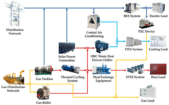
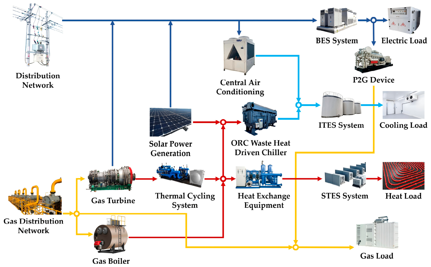
In accordance with the source-grid-load-storage architecture, as shown in Figure 1, this chapter establishes mathematical models for a rooftop PV system, gas turbine (GT) and gas boiler (GB), PV heating, waste-heat chiller driven by the ORC, central air conditioning (CAC), external grid interaction systems, ESS, EV loads, flexible loads, CCS and P2G systems, and LCT costs.

Figure 1. Overview of energy flows and major components in the IES.

These models are interconnected in terms of physical mechanisms and operational constraints, collectively constituting the constraints and components of the objective function for the subsequent optimal scheduling problem.

2.1. Mathematical Modeling of Integrated Energy System Equipment

Assume that there are n buildings within the low-carbon park-level IES, and the rooftop area available for PV power generation in each building is $S_i^{PVE}$. The rooftop PV system operates in maximum power point tracking (MPPT) mode, and its actual power generation $E_t^{PV}$ can be expressed as Equation (1):

$$\left\{\begin{array}{c}{E}_t^{PV}={\eta }_E^{PV}\cdot {\displaystyle \sum _{i=1}^n{I}_{i,t}^{PVE}}\cdot S_i^{PVE}\\ W^{PV}=P^{PV}\cdot {\displaystyle \sum _{t=1}^T{E}_t^{PV}}\end{array}\right.$$

(1)

where $I_{i,t}^{PVE}$ is average light intensity on i-th building PV array; ${\eta }_E^{PV}$ is cell energy conversion efficiency; $W^{PV}$ is PV system operating cost; $P^{PV}$ is unit electricity cost over PV life cycle; T is total scheduling duration. Max rooftop PV generation is proportional to light intensity. Meteorological factors cause light intensity uncertainty, making actual PV output $E_t^{PV}$ fluctuate around predicted $E_t^{PVpre}$.

Existing studies commonly model PV forecast errors as normally distributed, with a mean equal to the predicted value and a standard deviation proportional to the predicted value, reflecting larger absolute deviations at higher output levels. This assumption is physically motivated by the inherent heteroscedasticity of solar irradiance time series caused by weather events, as demonstrated in references [34,35]. The corresponding probability density function is given in Equation (2):

$$f(E_t^{PV})={\displaystyle \frac{1}{\beta E_t^{PVpre}\sqrt{2\mathrm{\pi }}}}\exp \left[-{\displaystyle \frac{{(E_t^{PV}-E_t^{PVpre})}^2}{2{(\beta E_t^{PVpre})}^2}}\right]$$

(2)

where $E_t^{PV}$ is the actual PV output, $E_t^{PVpre}$ is the predicted PV output, and β is the coefficient of variation, reflecting the relative magnitude of the forecast error.

In the multi-timescale progressive scheduling framework, the predicted PV output values between adjacent scales can be updated using Equation (3):

$$E_t^{PV,\mathit{new}}=E_t^{PV,\mathit{old}}+\Delta E_t^{PV}$$

(3)

where ${∆E}_t^{PV}~N(0,{\left(\beta E_t^{PV,old}\right)}^2)$, $E_t^{PV,old}$ is the predicted value from the previous scale, and $E_t^{PV,new}$ is the reference value at the current scale.

The GT is the core equipment of the CHP system, and its electric–thermal output exhibits coupling characteristics, while its operating status is influenced by start-up and shut-down actions. As demonstrated previously [2], its mathematical model can be expressed as Equation (4):

$$\left\{\begin{array}{l}{U}^{GT}{E}_{min}^{GT}\le E_t^{GT}\le U^{GT}{E}_{max}^{GT}\hfill \\ 0\le H_t^{GT}\le U^{GT}{H}_{max}^{GT}\hfill \\ E_t^{GT}\le U^{GT}{E}_0^{GT}+U^{GT}{k}_{up}\left(H_t^{GT}-H_{max}^{GT}\right)\hfill \\ E_t^{GT}\ge U^{GT}{E}_0^{GT}+U^{GT}{k}_{dn}\left(H_t^{GT}-H_{max}^{GT}\right)\hfill \\ U^{GT}\in \{0,1\}\hfill \end{array}\right.$$

(4)

where $E_t^{GT}$ and $H_t^{GT}$ are electric and thermal power output of GT; $E_{max}^{GT}$ and $E_{min}^{GT}$ are the upper and lower electric power output limits; $H_{max}^{GT}$ is the upper thermal power output; $E_0^{GT}$ is electric power at max thermal power output; $k_{up}$ and $k_{dn}$ are slope limits of electro-thermal coupling interval; $U^{GT}$ is GT on/off status.

The GT consumes the chemical energy of natural gas, converting part of it into electrical and thermal energy, while the remainder is recovered in the form of waste heat. Based on the energy balance principle, the relationship is established as Equation (5):

$$\left\{\begin{array}{l}{V}_t^{GT}={\displaystyle \frac{3.6\times {10}^6\cdot E_t^{GT}\cdot \Delta t}{{\eta }_e^{GT}\cdot Q_{\mathit{gas}}}}\hfill \\ {\displaystyle \frac{E_t^{GT}}{{\eta }_e^{GT}}}=E_t^{GT}+H_t^{GT}+H_t^{GT,\mathit{YR}}\hfill \\ V^{GT}={\displaystyle \sum _{t=1}^T{V}_t^{GT}}\hfill \end{array}\right.$$

(5)

where $V_t^{GT}$ is natural gas volume consumed by GT; Δt is single scheduling interval duration; ${\eta }_e^{GT}$ is GT electrical efficiency; $Q_{gas}$ is natural gas lower heating value; $H_t^{GT,YR}$ is GT waste heat recovery power; and $V^{GT}$ is total gas consumption over scheduling cycle.

GT startup and shutdown actions involve operating status changes between adjacent periods. To describe process linearly in optimization model, this paper introduces two independent auxiliary variable sets identifying startup and shutdown events. Constraints ensure mutual exclusivity in same period and precise correspondence to state changes. Specific constraints are expressed in Equation (6):

$$\left\{\begin{array}{ll}{U}_{\mathit{onoff},t}^{GT}=U_t^{GT}-U_{t+1}^{GT},\hfill & t=1,2,\dots ,T-1\hfill \\ U_{\mathit{onoff},t}^{GT}=U_{\mathit{on},t}^{GT}-U_{\mathit{off},t}^{GT}\hfill & \hfill \\ U_{\mathit{on},t}^{GT}+U_{\mathit{off},t}^{GT}\le 1\hfill & \hfill \\ U_{\mathit{on},t}^{GT},U_{\mathit{off},t}^{GT}\in \{0,1\}\hfill & \hfill \\ U_{\mathit{onoff},T}^{GT}=0\hfill & \hfill \end{array}\right.$$

(6)

where $U_t^{GT}$ is the on/off status variable; $U_{onoff,t}^{GT}$ is the status change between adjacent periods; $U_{on,t}^{GT}$ is the start-up action indicator; and $U_{off,t}^{GT}$ is the shut-down action indicator.

The total operating cost of the GT, denoted as $W^{GT}$, encompasses two components: startup and shutdown cost $W_{onoff}^{GT}$ and maintenance cost $W_{wh}^{GT}$. Meanwhile, carbon emissions $m^{GT}$ are proportional to total gas consumption, with the specific expressions detailed in Equation (7):

$$\left\{\begin{array}{l}{W}_{\mathit{onoff}}^{GT}={\displaystyle \sum _{t=1}^T\left(U_{\mathit{on},t}^{GT}\cdot p_{\mathit{on}}^{GT}+U_{\mathit{off},t}^{GT}\cdot p_{\mathit{off}}^{GT}\right)}\hfill \\ W_{\mathit{wh}}^{GT}={\displaystyle \sum _{t=1}^T\left(p_e^{GT}\cdot E_t^{GT}+p_h^{GT}\cdot H_t^{GT}\right)}\hfill \\ W^{GT}=W_{\mathit{onoff}}^{GT}+W_{\mathit{wh}}^{GT}\hfill \\ m^{GT}={\xi }_{\mathit{gas}}\cdot V^{GT}\hfill \end{array}\right.$$

(7)

$p_{on}^{GT}$ and $p_{off}^{GT}$ are start-up and shut-down costs. $p_e^{GT}$ and $p_h^{GT}$ are maintenance costs per unit electricity and heat production; ${\xi }_{gas}$ is CO₂ emission coefficient per unit natural gas combustion volume. GB provides supplementary thermal power when GT heat supply is insufficient or during peak load regulation. Operation involves one-way conversion of fuel chemical energy into thermal energy with partial waste heat dissipation. Based on previous research [3], the quantitative relationship is expressed as Equation (8):

$$\left\{\begin{array}{l}{V}_t^{\mathit{GB}}={\displaystyle \frac{3.6\times {10}^6\cdot H_t^{\mathit{GB}}\cdot \Delta t}{{\eta }^{\mathit{GB}}\cdot Q_{\mathit{gas}}}}\hfill \\ H_t^{\mathit{GB},\mathit{YR}}=\left({\displaystyle \frac{1-{\eta }^{\mathit{GB}}}{{\eta }^{\mathit{GB}}}}\right)H_t^{\mathit{GB}}\hfill \\ m^{\mathit{GB}}={\xi }_{\mathit{gas}}\cdot {\displaystyle \sum _{t=1}^T{V}_t^{\mathit{GB}}}\hfill \\ W^{\mathit{GB}}=p_h^{GB}\cdot {\displaystyle \sum _{t=1}^T{H}_t^{\mathit{GB}}}\hfill \end{array}\right.$$

(8)

where $H_t^{GB}$ is GB thermal power output; $V_t^{GB}$ is natural gas volume consumed by GB; ${\eta }^{GB}$ is GB thermal efficiency; $H_t^{GB,YR}$ is GB waste heat recovery power; $m^{GB}$ is total GB CO₂ emissions; $p_h^{GB}$ is the unit operational cost price; and $W^{GB}$ is GB operating cost.

GT and GB operation generates waste heat, causing energy waste if emitted. Rooftop PV power converts directly to thermal energy besides electricity. Combining PV thermal production with gas-fired equipment waste heat recovery drives the ORC-powered waste heat chiller to achieve heat-to-cooling conversion for park cooling demand. According to research [8], the coupling model of PV thermal production and PV-ORC waste heat cooling is established as shown in Equation (9):

$$\left\{\begin{array}{l}{H}_t^{PV}={\eta }_H^{PV}\cdot {\displaystyle \sum _{i=1}^m\left(I_{i,t}^{\mathit{PVH}}\cdot S_i^{\mathit{PVH}}\right)}\hfill \\ L_t^{\mathit{ORC}}={\eta }_L^{\mathit{ORC}}\cdot H_t^{\mathit{ORC}}\hfill \\ H_t^{\mathit{ORC}}\le H_t^{PV}+H_t^{GT,\mathit{YR}}+H_t^{\mathit{GB},\mathit{YR}}\hfill \\ W^{\mathit{ORC}}=p^{\mathit{ORC}}\cdot {\displaystyle \sum _{t=1}^T{L}_t^{\mathit{ORC}}}\hfill \end{array}\right.$$

(9)

where $H_t^{PV}$ is PV thermal production power; ${\eta }_H^{PV}$ is PV array heat absorption efficiency; $I_{i,t}^{PVH}$ is average light intensity on i-th building heat absorption PV array; $S_i^{PVH}$ is area of i-th building heat absorption PV array; $L_t^{ORC}$ is cooling power of the ORC waste heat chiller; ${\eta }_L^{ORC}$ is thermal to cooling conversion efficiency of the ORC waste heat chiller; $H_t^{ORC}$ is ORC chiller heat consumption; $H_t^{GT,YR}$ is GT waste heat recovery power; $H_t^{GB,YR}$ is GB waste heat recovery power; $p^{ORC}$ is operating cost per unit cooling power of the ORC waste heat chiller; and $W^{ORC}$ is operating cost of the ORC waste heat chiller over entire scheduling horizon T. The ORC waste heat chiller cooling capacity is limited by waste heat temperature level. Insufficient waste heat or sudden cooling load surges require an electric-driven refrigeration equipment supplement.

As an electric cooling and heating device, CAC features fast response and flexible regulation, serving as important supplementary means for park cooling and heating load balancing. The following section establishes a CAC dual-mode operation model, as shown in Equation (10):

$$\left\{\begin{array}{l}{L}_t^{\mathit{EL}}={\eta }_L^{\mathit{EL}}\cdot E_t^{\mathit{EL}}\hfill \\ H_t^{\mathit{EH}}={\eta }_H^{\mathit{EH}}\cdot E_t^{\mathit{EH}}\hfill \\ 0\le L_t^{\mathit{EL}}\le {\delta }_t^{\mathit{EH}}\cdot L_{\mathit{max}}^{\mathit{EL}}\hfill \\ 0\le H_t^{\mathit{EH}}\le (1-{\delta }_t^{\mathit{EH}})\cdot H_{\mathit{max}}^{\mathit{EH}}\hfill \\ 0\le E_t^{\mathit{EL}}\le {\delta }_t^{\mathit{EH}}\cdot {\displaystyle \frac{L_{\mathit{max}}^{\mathit{EL}}}{{\eta }_L^{\mathit{EL}}}}\hfill \\ 0\le E_t^{\mathit{EH}}\le (1-{\delta }_t^{\mathit{EH}})\cdot {\displaystyle \frac{H_{\mathit{max}}^{\mathit{EH}}}{{\eta }_H^{\mathit{EH}}}}\hfill \\ {\delta }_t^{\mathit{EH}}\in \{0,1\}\hfill \end{array}\right.$$

(10)

where $L_t^{EL}$ is CAC cooling power; $H_t^{EL}$ is CAC heating power; $E_t^{EL}$ is CAC electric power consumption for cooling; $E_t^{EH}$ is CAC electric power consumption for heating; ${\eta }_t^{EL}$ is electric-to-cooling conversion efficiency; ${\eta }_t^{EH}$ is electric-to-heating conversion efficiency; $L_{max}^{EL}$ is cooling power upper limit; $H_{max}^{EH}$ is heating power upper limit; and ${\delta }_t^{EH}$ is the operation mode indicator.

The low-carbon park-level IES is connected to the distribution network through a transformer, and the transformer capacity determines the upper limit of the interactive power. Electricity purchasing and selling behaviors cannot occur simultaneously, and the power of each should not exceed the allowable interaction limit of the transformer. The mathematical model is given in Equation (11):

$$\left\{\begin{array}{l}0\le E_t^{\mathit{buy}}\le E_{\mathit{max}}^{\mathit{Grid}}\cdot {\delta }_t^{\mathit{Grid}}\hfill \\ 0\le E_t^{\mathit{sell}}\le E_{\mathit{max}}^{\mathit{Grid}}\cdot (1-{\delta }_t^{\mathit{Grid}})\hfill \\ {\delta }_t^{\mathit{Grid}}\in \{0,1\}\hfill \end{array}\right.$$

(11)

where $E_t^{buy}$ and $E_t^{sell}$ are power purchased from and sold to the distribution network; $E_{max}^{Grid}$ is the transformer-constrained interactive power upper limit; and ${\delta }_t^{Grid}$ is an interactive state variable. Due to internal sources like PV and GT, surplus electricity exists; thus, grid interaction cost involves both purchase expenditures and sales revenue, expressed in Equation (12):

$$W^{\mathit{EGrid}}={\displaystyle {\displaystyle \sum _{t=1}^T}{p}_t^{\mathit{Ebuy}}}\cdot E_t^{\mathit{buy}}-{\displaystyle {\displaystyle \sum _{t=1}^T}{p}_t^{\mathit{Esell}}}\cdot E_t^{\mathit{sell}}$$

(12)

where $W^{EGrid}$ is the grid power exchange cost; $p_t^{Ebuy}$ is TOU price for purchasing electricity; and $p_t^{Esell}$ is TOU price for selling electricity.

Natural gas required by the IES follows a buy-and-use principle relying on external gas networks. The model is shown in Equation (13):

$$0\le G_t^{\mathit{buy}}\le G_{\mathit{max}}^{\mathit{Grid}}$$

(13)

where $G_t^{buy}$ is natural gas power purchased from the gas distribution network; $G_{max}^{Grid}$ is the gas purchase power upper limit. Total gas cost over dispatch period T is modeled as Equation (14):

$$W^{\mathit{GGrid}}=p^{\mathit{Gbuy}}\cdot {\displaystyle \sum _{t=1}^T{G}_t^{\mathit{buy}}}$$

(14)

where $p^{Gbuy}$ is the unit price of natural gas purchased; $W^{GGrid}$ is the total cost of purchasing gas from the gas distribution network over the dispatch period T.

The random fluctuation of PV output, the peak-valley difference of loads, and the TOU electricity price mechanism make energy storage a key means to improve the operational economy and reliability of the system. Although battery energy storage (BES), solid thermal energy storage (STES), and ice thermal energy storage (ITES) involve distinct physical media, their scheduling models exhibit structurally homogeneous characteristics. Consequently, this subsection establishes a unified mathematical framework for the three types, where BES corresponds to the electricity storage domain, STES to the heat storage domain, and ITES to the cooling storage domain. This unified framework enables the temporal shifting of electricity, heat, and cooling energy through a single set of constraints, with specific characteristics distinguished through parameterization and auxiliary equipment equations.

The operating states of the energy storage systems at any moment are mutually exclusive, and their charging and discharging powers are simultaneously constrained by the rated capacities and state variables. In the model proposed by reference [10], the unified power boundary model is shown in Equation (15):

$$\left\{\begin{array}{l}0\le P_t^{\mathit{sysC}}\le P_{\max }^{\mathit{sysC}}\cdot u_t^{\mathit{sysC}}\hfill \\ 0\le P_t^{\mathit{sysD}}\le P_{\max }^{\mathit{sysD}}\cdot u_t^{\mathit{sysD}}\hfill \\ u_t^{\mathit{sysC}}+u_t^{\mathit{sysD}}\le 1\hfill \\ u_t^{\mathit{sysC}},u_t^{\mathit{sysD}}\in \{0,1\}\hfill \end{array}\right.$$

(15)

where the superscript sys serves as a placeholder for the three storage types. The variables $P_t^{sysC}$ and $P_t^{sysD}$ represent the charging and discharging power of the storage system, respectively. In physical terms, this unified power variable denotes electric power (E) for the BES system, thermal power (H) for the STES system, and cooling power (L) for the ITES system. The terms $P_{max}^{sysC}$ and $P_{max}^{sysD}$ denote the upper limits of charging and discharging power. The binary indicators $u_t^{sysC}$ and $u_t^{sysD}$ ensure that charging and discharging never occur simultaneously.

The recursive relationship of the stored energy level across multiple time periods accounts for self-loss and conversion efficiencies. The unified model is shown in Equation (16):

$$S_{t+1}^{\mathit{sys}}=(1-{\eta }_{\mathit{loss}}^{\mathit{sys}})\cdot S_t^{\mathit{sys}}+{\eta }^{\mathit{sysC}}\cdot P_t^{\mathit{sysC}}\cdot \Delta t-{\displaystyle \frac{P_t^{\mathit{sysD}}}{{\eta }^{\mathit{sysD}}}}\cdot \Delta t$$

(16)

where $S_t^{sys}$ represents the stored energy level of the system. The coefficient ${\eta }_{loss}^{sys}$ represents the self-loss coefficient. The terms ${\eta }^{sysC}$ and ${\eta }^{sysD}$ are the charging and discharging efficiencies.

To ensure energy balance over the dispatch period and operational feasibility, the storage level must remain within physical bounds, and the terminal state must equal the initial state. These constraints are expressed in Equation (17):

$$\left\{\begin{array}{l}{S}_{\mathit{min}}^{\mathit{sys}}\le S_t^{\mathit{sys}}\le S_{\mathit{max}}^{\mathit{sys}},\hspace{0.33em}\hspace{0.33em}\hspace{0.33em}\forall t\in [1,T]\hfill \\ S_0^{\mathit{sys}}=S_T^{\mathit{sys}}\hfill \end{array}\right.$$

(17)

where $S_{min}^{sys}$ and $S_{max}^{sys}$ are the lower and upper limits of the stored energy. The terms $S_0^{sys}$ and $S_T^{sys}$ represent the stored energy at the beginning and end of the dispatch period, ensuring periodicity.

The specific parameter values for each storage type within the unified framework are listed in Table 1.

Table 1. Parameter mapping for the unified energy storage model.

Variable Description	Symbol	BES	STES	ITES
Unified power variable	$P_t^{sys}$	$E_t^{BES}$	$H_t^{STES}$	$L_t^{ITES}$
Stored energy variable	$S_t^{sys}$	$S_t^{BES}$	$S_t^{STES}$	$S_t^{ITES}$
Self-loss coefficient	${\eta }_{loss}^{sys}$	${\eta }_{loss}^{BES}$	${\eta }_{loss}^{STES}$	${\eta }_{loss}^{ITES}$
Charging efficiency	${\eta }^{sysC}$	${\eta }^{BESC}$	${\eta }^{STESC}$	${\eta }^{ITESC}$
Discharging efficiency	${\eta }^{sysD}$	${\eta }^{BESD}$	${\eta }^{STESD}$	${\eta }^{ITESD}$
Minimum stored energy	$S_{min}^{sys}$	$S_{min}^{BES}$	$S_{min}^{STES}$	$S_{min}^{ITES}$
Maximum stored energy	$S_{max}^{sys}$	$S_{max}^{BES}$	$S_{max}^{STES}$	$S_{max}^{ITES}$
Unit depreciation cost	$p_{unit}^{sys}$	$p_{unit}^{BES}$	$p_{unit}^{STES}$	$p_{unit}^{ITES}$

The total depreciation cost over the entire dispatch period is uniformly formulated as Equation (18):

$$W^{\mathit{sys}}={\displaystyle \sum _{t=1}^T{p}_{\mathit{unit}}^{\mathit{sys}}}\cdot \left(P_t^{\mathit{sysC}}+P_t^{\mathit{sysD}}\right)\cdot \Delta t$$

(18)

where $W^{sys}$ represents the depreciation cost of each specific storage system, and $p_{unit}^{sys}$ denotes the unit depreciation cost per power throughput for the charging and discharging operations.

Within the unified framework, STES and ITES introduce specific auxiliary equipment during their operation. For STES, the blower is required as auxiliary equipment during the thermal discharging process. The blower expels high-temperature air. The power consumption of the blower is modeled as Equation (19):

$$E_t^{\mathit{STESD}}={\xi }^{\mathit{STESD}}\cdot H_t^{\mathit{STESD}}$$

(19)

where $E_t^{STESD}$ represents the electric power consumption of the blower. The parameter ${\xi }^{STESD}$ is the coefficient of electric power consumption per unit of thermal discharging power.

For ITES, the ice-melting process similarly necessitates the operation of water pumps during the discharging phase. The power consumption of these auxiliary devices is modeled as Equation (20):

$$E_t^{\mathit{ITESD}}={\xi }^{\mathit{ITESD}}\cdot L_t^{\mathit{ITESD}}$$

(20)

where $E_t^{ITESD}$ represents the electric power consumption of the water pump, and ${\xi }^{ITESD}$ is the coefficient of electric power consumption per unit of cooling discharging power.

2.2. Mathematical Modeling of Flexible Load Demand Response

2.2.1. Modeling of Electric Vehicle Load

Besides energy storage equipment, user-side flexible loads have energy time-shifting potential. As important dispatchable load resource in park, EV charging behavior can be guided by price signals. Inspired by previous research [12], a large-scale EV charging load model was constructed using a Monte Carlo stochastic simulation method combined with random variable transformation and inverse cumulative distribution function transformation. The modeling process included basic premises, as follows: EV travel patterns match traditional fuel vehicles; each EV charges once daily uniformly, adopting the rated power of AC slow charging in the community parking lot; charging pile facilities in the area are sufficient; with a total of 1750 EVs, 50% of users participate in DR. Daily driving distance $S_i^{EV}$ of i-th EV can be obtained from the standard normal random variable $Z_{s,i}~N(0,1)$ through exponential transformation, as shown in Equation (21):

$$S_i^{\mathit{EV}}=\exp ({\mu }_d+{\sigma }_d\cdot Z_{s,i})$$

(21)

where $u_d$ = 3.2, ${\sigma }_d$ = 0.88. The corresponding probability density function is derived through variable transformation, given by Equation (22):

$$f_S(x)={\displaystyle \frac{1}{x{\sigma }_d\sqrt{2\pi }}}\exp \left(-{\displaystyle \frac{{(\ln x-{\mu }_d)}^2}{2{\sigma }_d^2}}\right),\hspace{1em}x>0$$

(22)

where $Z_{s,i}$ is a random perturbation following a standard normal distribution, $u_d$ is the logarithmic mean, and ${\sigma }_d$ is the logarithmic standard deviation.

The moment when the EV returns and starts charging, $T_i^{EVCS}$, is regarded as a random variable in circular time and is described by the wrapped normal distribution, as shown in Equation (23):

$$\begin{array}{l}{T}_i^{\mathit{EVCS}}=\left({\mu }_t+{\sigma }_t\cdot Z_{t,i}\right)\hspace{1em}\hspace{1em}\mathrm{mod}\hspace{0.17em}24\hfill \end{array}$$

(23)

where $Z_{t,i}~N(0,1)$, $u_t$ = 17.6, ${\sigma }_t$ = 3.4. Its probability density function is an infinite series on the circle, given by Equation (24):

$$f_T(x)={\displaystyle \frac{1}{{\sigma }_t\sqrt{2\pi }}}{\displaystyle \sum _{k=-\infty }^{\infty }\exp }\left(-{\displaystyle \frac{{(x-{\mu }_t+24k)}^2}{2{\sigma }_t^2}}\right),\hspace{1em}0\le x<24$$

(24)

where $Z_{t,i}$ is a standard normal random variable, $u_t$ is the linear mean of the starting time, ${\sigma }_t$ is the standard deviation.

The charging duration of the i-th EV after daily driving, denoted as $T_i^{EVCL}$, is determined by the ratio of the electricity consumed during the day’s driving to the charging power. The equivalent energy consumption rate is defined as ${\alpha }_i$, which converts the electricity consumption per 100 km and the charging efficiency into the equivalent electric energy required per kilometer of driving. The calculation formula for charging duration and the variable definitions are presented in Equation (25):

$$\left\{\begin{array}{l}{\alpha }_i={\displaystyle \frac{W_i^{\mathit{EV}100}}{100\cdot {\eta }_i^{\mathit{EVC}}}}\hfill \\ T_i^{\mathit{EVCL}}={\displaystyle \frac{{\alpha }_i\cdot S_i^{\mathit{EV}}}{E_i^{\mathit{EVC}}}}\hfill \end{array}\right.$$

(25)

where $S_i^{EV}$ is the daily driving distance of the i-th EV; $W_i^{EV100}$ is the electricity consumption per 100 km for this vehicle model; $E_i^{EVC}$ is the average charging power; and ${\eta }_i^{EVC}$ is the charging efficiency.

To fully exploit the peak-shaving and valley-filling potential of large-scale EV loads, this paper establishes a DR model based on the differential form of the elastic electricity price. The electricity price change rate ${\delta }_t^{EV}$ is defined as shown in Equation (26):

$${\delta }_t^{\mathit{EV}}={\displaystyle \frac{\Delta P_t^{\mathit{EV}}}{P_t^{\mathit{EVO}}}},\hspace{1em}\forall t$$

(26)

where $∆P_t^{EV}$ is the change in electricity price, and $P_t^{EVO}$ is the original electricity price.

As presented in previous research [15], the relative change in EV load power is associated with the elasticity coefficient matrix ${\mathbf{R}}^{EV}$ as shown in Equation (27):

$${\displaystyle \frac{\Delta E_t^{\mathit{EV}}}{E_t^{\mathit{EVO}}}}={\displaystyle \sum _{s=1}^T{R}_{t,s}^{\mathit{EV}}}\cdot {\displaystyle \frac{\Delta P_s^{\mathit{EV}}}{P_s^{\mathit{EVO}}}},\hspace{1em}\forall t$$

(27)

where $∆E_t^{EV}$ is the change in EV load power, $E_t^{EVO}$ is the original EV load power, and $R_{t,s}^{EV}$ is an element of the elasticity coefficient matrix, representing the influence coefficient of the electricity price change. This formula can be expressed in matrix form as Equation (28):

$$\left\{\begin{array}{l}\Delta e=\mathrm{diag}(E^{\mathit{EVO}})\cdot R^{\mathit{EV}}\cdot \left(\mathrm{diag}{(P^{\mathit{EVO}})}^{-1}\Delta p\right)\hfill \\ \Delta e={\left[\Delta E_1^{\mathit{EV}}\hspace{0.33em}\Delta E_2^{\mathit{EV}}\hspace{0.33em}\dots \Delta E_T^{\mathit{EV}}\right]}^T\hfill \\ \Delta p={\left[\Delta P_1^{\mathit{EV}}\hspace{0.33em}\Delta P_2^{\mathit{EV}}\hspace{0.33em}\dots \Delta P_T^{\mathit{EV}}\right]}^T\hfill \end{array}\right.$$

(28)

where $∆\mathbf{e}$ is the power change vector, $∆\mathbf{p}$ is the electricity price change vector, ${\mathbf{E}}^{EVO}$ is the original power vector, and ${\mathbf{P}}^{EVO}$ is the original electricity price vector. The final power and electricity price after dispatch satisfy Equation (29):

$$\left\{\begin{array}{l}{E}_t^{\mathit{EV}}=E_t^{\mathit{EVO}}+\Delta E_t^{\mathit{EV}}\hfill \\ P_t^{\mathit{EV}}=P_t^{\mathit{EVO}}+\Delta P_t^{\mathit{EV}}\hfill \end{array}\right.$$

(29)

where $E_t^{EV}$ is the EV load power after response, and $P_t^{EV}$ is the electricity price after response.

The EV load is essentially a TL, and the total electricity consumption across all periods is conserved before and after the response, as shown in Equation (30):

$${\displaystyle \sum _{t=1}^T\Delta }{E}_t^{\mathit{EV}}=0$$

(30)

The total charging costs before and after participating in DR, respectively, are calculated as shown in Equation (31):

$$\left\{\begin{array}{l}{W}^{\mathit{EVO}}={\displaystyle \sum _{t=1}^T{E}_t^{\mathit{EVO}}}{P}_t^{\mathit{EVO}}\Delta t\hfill \\ W^{\mathit{EV}}={\displaystyle \sum _{t=1}^T{E}_t^{\mathit{EV}}}{P}_t^{\mathit{EV}}\Delta t\hfill \end{array}\right.$$

(31)

where $W^{EVO}$ is the total charging cost before response, and $W^{EV}$ is the total charging cost after response.

User satisfaction is defined by the charging cost saving rate; the larger the $M^{EV}$, the higher the user satisfaction, as shown in Equation (32):

$$\left\{\begin{array}{l}{M}^{\mathit{EV}}=1-{\displaystyle \frac{W^{\mathit{EV}}}{W^{\mathit{EVO}}}}\hfill \\ M^{\mathit{EV}}\ge 0\hfill \end{array}\right.$$

(32)

2.2.2. Modeling of Curtailable and Transferable Loads

In addition to EVs, the park has CLs including CTCLs and TLs from industrial or residential sectors. The former curtails power by adjusting indoor temperature setpoints; the latter shifts power inter-periodically assuming unchanged total daily consumption. DR models for CTCLs and TLs are established. First, baseline thermostatically controlled load (BTCL) power without DR is defined. Outdoor temperature and BTCL determine ideal indoor temperature, as shown in Equation (33):

$$F_t^{\mathit{set}}=F_t^O+{\eta }_H^F\cdot H_t^{\mathit{Fset}}-{\eta }_L^F\cdot L_t^{\mathit{Fset}}$$

(33)

where $F_t^{set}$ is the indoor ideal temperature, $F_t^O$ is the outdoor temperature, ${\eta }_H^F$ and ${\eta }_L^F$ are the conversion coefficients of heating and cooling load-to-room temperature, and $H_t^{Fset}$ and $L_t^{Fset}$ are the baseline heating load power and baseline cooling load power.

When participating in DR, the actual operating power of TCLs is lower than the baseline value, thereby causing room temperature deviation. The actual room temperature can be expressed as shown in Equation (34):

$$F_t=F_t^O+{\eta }_H^F\cdot H_t^F-{\eta }_L^F\cdot L_t^F$$

(34)

where $H_t^F$ and $L_t^F$ are the actual heating and cooling power of TCLs.

From Equations (33) and (34), the relationship between the room temperature deviation and the load curtailment amount $∆F_t$ can be obtained, as shown in Equation (35):

$$\Delta F_t\triangleq F_t^{\mathit{set}}-F_t={\eta }_H^F(H_t^{\mathit{Fset}}-H_t^F)+{\eta }_L^F(L_t^F-L_t^{\mathit{Fset}})$$

(35)

User comfort requires that the room temperature deviation must not exceed the allowable upper limit $F_{lim}$, and the heating and cooling power of CTCLs is constrained by their physical upper limits $H_{max}^F$ and $L_{max}^F$, as expressed in Equation (36):

$$\left\{\begin{array}{l}|\Delta F_t|\le F_{\mathit{lim}}\hfill \\ 0\le H_t^F\le H_{\mathit{max}}^F\hfill \\ 0\le L_t^F\le L_{\mathit{max}}^F\hfill \end{array}\right.$$

(36)

User indoor temperature satisfaction $M^{TC}$ is directly associated with the room temperature deviation and must be maintained above a set threshold. Its definition and constraints are as shown in Equation (37):

$$\left\{\begin{array}{l}{M}^{\mathit{TC}}=1-{\displaystyle \frac{|\Delta F_t|}{F_t^{\mathit{set}}}}\hfill \\ M^{\mathit{TC}}\ge 0.8\hfill \end{array}\right.$$

(37)

In the model proposed by reference [11], total CTCL is defined as the sum of heating load curtailment and cooling load curtailment, and the dispatch center provides compensation based on the cumulative curtailment amount, as shown in Equation (38):

$$\left\{\begin{array}{l}\Delta H_t^F=(H_t^{\mathit{Fset}}-H_t^F)+(L_t^{\mathit{Fset}}-L_t^F)\hfill \\ W^F={\xi }^F\cdot {\displaystyle \sum _{t=1}^T\Delta }{H}_t^F\hfill \end{array}\right.$$

(38)

where $∆H_t^F$ is the curtailment amount of TCLs, ${\xi }^F$ is the compensation unit price per unit curtailment, and $W^F$ is the CTCL DR compensation cost.

The total electricity consumption of TLs remains unchanged over the dispatch period, but the power in each period can be flexibly adjusted. This model describes the response behavior using the form of a load shifting matrix. First, the total electricity consumption before and after the response is conserved, as shown in Equation (39):

$${\displaystyle {\displaystyle \sum _{t=1}^T}{E}_t^{\mathit{TL}}}={\displaystyle {\displaystyle \sum _{t=1}^T}{E}_t^{\mathit{TLO}}}$$

(39)

where $E_t^{TL}$ and $E_t^{TLO}$ are the transferable load power after and before response.

Define the load change in each period as $∆E_t^{TL}$; then, the conservation constraint of total electricity consumption is equivalent to Equation (40):

$$\left\{\begin{array}{l}\Delta E_t^{\mathit{TL}}=E_t^{\mathit{TL}}-E_t^{\mathit{TLO}}\hfill \\ {\displaystyle \sum _{t=1}^T\Delta }{E}_t^{\mathit{TL}}=0\hfill \end{array}\right.$$

(40)

To evaluate the impact of transferable loads on the peak-valley difference of the system, the non-transferable constant load $E_t^{LoadO}$ is introduced. The total system loads before and after the response are shown in Equation (41):

$$\left\{\begin{array}{l}{E}_t^{\mathit{LoadTLO}}=E_t^{\mathit{LoadO}}+E_t^{\mathit{TLO}}\hfill \\ E_t^{\mathit{LoadTL}}=E_t^{\mathit{LoadO}}+E_t^{\mathit{TL}}\hfill \end{array}\right.$$

(41)

where $E_t^{LoadTLO}$ and $E_t^{LoadTL}$ are the total power consumption including the constant load before and after response.

The peak-shaving effect of transferable loads is defined as the reduction in the peak value of the total load before and after response, as shown in Equation (42). The compensation that users receive for participating in load shifting is proportional to the peak-shaving amount.

$$\left\{\begin{array}{l}{A}^{\mathit{TL}}=\max (E_t^{\mathit{LoadTLO}})-\max (E_t^{\mathit{LoadTL}})\hfill \\ W^{\mathit{TL}}={\zeta }^{\mathit{TL}}\cdot A^{\mathit{TL}}\hfill \end{array}\right.$$

(42)

where $A^{TL}$ is the peak load reduction amount, ${\zeta }^{TL}$ is the compensation coefficient per unit reduction, and $W^{TL}$ is the total compensation cost for transferable loads.

2.3. Modeling of Power-to-Gas Conversion Facilities and Carbon Trading Mechanisms

Previous models have focused on energy production, conversion, storage, and consumption. Meanwhile, carbon emissions have become critical in park operation under carbon peak and neutrality targets. Introducing CCS and P2G systems enables carbon recycling. CCS is key to reducing emissions in low-carbon park IES. It captures CO₂ from GT and GB flue gas; after compression and transport, CO₂ is used in P2G or sequestered. CCS reduces net emissions and LCT cost. A mathematical model of CCS is given in Equation (43):

$$\left\{\begin{array}{l}{M}_t^{\mathit{CC}}\le {\eta }_{\mathit{CC}}\cdot {\xi }_{\mathit{gas}}\left(V_t^{GT}+V_t^{\mathit{GB}}\right)\hfill \\ E_t^{\mathit{CC}}={\beta }_{\mathit{CC}}\cdot M_t^{\mathit{CC}}\hfill \\ 0\le E_t^{\mathit{CC}}\le E_{\mathit{max}}^{\mathit{CC}}\hfill \\ W^{\mathit{CC}}=p^{\mathit{CC}}\cdot {\displaystyle \sum _{t=1}^T{E}_t^{\mathit{CC}}}\hfill \end{array}\right.$$

(43)

where $M_t^{CC}$ is mass of CO₂ captured by CCS; ${\eta }_{CC}$ is capture efficiency; $V_t^{GT}$ and $V_t^{GB}$ are the volumes of natural gas consumed by the GT and GB, respectively; $E_t^{CC}$ is CCS power consumption; ${\beta }_{CC}$ is the unit electricity consumption coefficient; $E_{max}^{CC}$ is the maximum power limit; $W^{CC}$ is the CCS operating cost; and $p^{CC}$ is cost per unit of electricity. Drawing on previous research [25], the P2G system utilizes surplus electricity for hydrogen production through electrolysis, reacting with CCS-captured CO₂ by methanation to synthesize natural gas. Synthesized natural gas is injected into the gas network or supplied to GTs and GBs, enabling long-term energy storage and carbon recycling. The mathematical model of a P2G system is expressed as Equation (44):

$$\left\{\begin{array}{l}{M}_t^{P2G}\le M_t^{\mathit{CC}}\hfill \\ M_t^{P2G}=k_{P2G}\cdot V_t^{P2G}\hfill \\ V_t^{P2G}={\displaystyle \frac{E_t^{P2G}\cdot {\eta }_{P2G}\cdot 3.6}{Q_{\mathit{gas}}/{10}^6}}\hfill \\ 0\le E_t^{P2G}\le E_{\mathit{max}}^{P2G}\hfill \\ W^{P2G}=p^{P2G}\cdot {\displaystyle \sum _{t=1}^T{E}_t^{P2G}}\hfill \\ G_t^{P2G}=V_t^{P2G}\cdot Q_{\mathit{gas}}\hfill \end{array}\right.$$

(44)

where $M_t^{P2G}$ is CO₂ mass consumed by P2G; $k_{P2G}$ is CO₂ consumption coefficient per unit gas volume; $G_t^{P2G}$ is power of P2G-generated natural gas; $V_t^{P2G}$ is P2G-generated gas volume; $E_t^{P2G}$ is P2G power consumption; ${\eta }_{P2G}$ is P2G conversion efficiency; $Q_{gas}$ is natural gas lower heating value; $E_{max}^{P2G}$ is maximum P2G power limit; $W^{P2G}$ is total P2G operating cost; and $p^{P2G}$ is electricity cost per unit.

Introducing CCS and P2G alters net carbon emissions, affecting carbon trading costs. GTs and GBs are the main CO₂ sources in this low-carbon park IES. To incentivize reduction, the LCT mechanism is adopted. Unlike fixed prices, this mechanism uses progressive price factors based on emission levels; higher emissions increase unit costs, while reductions yield higher benefits. The net emissions $m_{net}$ formula is given in Equation (45):

$$m_{\mathit{net}}={\xi }_{\mathit{gas}}{\displaystyle {\displaystyle \sum _{t=1}^T}\left(V_t^{GT}+V_t^{\mathit{GB}}\right)}-{\displaystyle {\displaystyle \sum _{t=1}^T}{M}_t^{P2G}}$$

(45)

where $m_{net}$ is the total net carbon emissions of the system over the entire dispatch period.

According to reference [13], the piecewise function expression of the LCT cost $W^{CE}$ can be expressed as Equation (46):

$$W^{CE}=\left\{\begin{array}{ll}-c_0{\displaystyle \sum _{i=1}^{k-1}{\gamma }^{i-1}}d-c_0{\gamma }^{k-1}(|m_{net}|-(k-1)d),\hfill & -kd<m_{net}\le -(k-1)d,\hspace{1em}k=2,\dots ,K\hfill \\ -c_0\left|m_{net}\right|,\hfill & -d<m_{net}\le 0\hfill \\ c_0{m}_{net},\hfill & 0<m_{net}\le d\hfill \\ c_0{\displaystyle \sum _{i=0}^{k-2}{\gamma }^i}d+c_0{\gamma }^{k-1}(m_{net}-kd),\hfill & kd<m_{net}\le (k+1)d,\hspace{1em}k=2,\dots ,K-1\hfill \end{array}\right.$$

(46)

where $W^{CE}$ is the LCT cost; $m_{net}$ is the net carbon emissions of the system; $c_0$ is the carbon trading base price; d is the ladder interval length; γ is the ladder price growth factor; and K is a positive integer representing the maximum number of ladder intervals.

2.4. Multiphase Flow Coupled Equations of Equilibrium Constraints

In summary, this chapter establishes a mathematical model for low-carbon park IES, covering PV, GTs, GBs, PV heating, ORC cooling, CAC, grid interaction, storage, EVs, flexible loads, CCS, P2G, and LCT. Sub-models focus on power balance, efficiency, constraints, and costs, forming the basis for optimization. IES involves electricity, gas, heat, and cooling flows. Device conversions were previously modeled. Electricity supply–demand balance is shown in Equation (47):

$$\begin{array}{l}{E}_t^{\mathit{buy}}+E_t^{GT}+E_t^{PV}+E_t^{\mathit{BESD}}=E_t^{\mathit{EL}}+E_t^{\mathit{EH}}+E_t^{\mathit{sell}}+E_t^{\mathit{BESC}}\\ +E_t^{\mathit{EVO}}+\Delta E_t^{\mathit{EV}}+E_t^{\mathit{TLO}}+\Delta E_t^{\mathit{TL}}+E_t^{\mathit{LoadO}}+E_t^{\mathit{STESD}}+E_t^{\mathit{ITESD}}+E_t^{\mathit{CC}}+E_t^{P2G}\end{array}$$

(47)

where $E_t^{buy}$ and $E_t^{sell}$ are IES power purchased from and sold to the distribution network; $E_t^{GT}$ is GT power generation; $E_t^{PV}$ is PV generation; $E_t^{BESC}$ and $E_t^{BESD}$ are BES charging and discharging power; $E_t^{EL}$ and $E_t^{EH}$ are CAC power for cooling and heating; $E_t^{EVO}$ and $∆E_t^{EV}$ are EV baseline load and variation under elastic prices; $E_t^{TLO}$ and $∆E_t^{TL}$ are TL baseline and variation after DR; $E_t^{LoadO}$ is constant load; and $E_t^{CC}$ and $E_t^{P2G}$ are CCS and P2G power consumption.

The heating supply–demand balance is modeled as shown in Equation (48):

$$H_t^{GT}+H_t^{PV}+H_t^{\mathit{GB}}+H_t^{\mathit{STESD}}=H_t^{\mathit{ORC}}+H_t^{\mathit{STESC}}+H_t^F+H_t^{\mathit{LoadO}}$$

(48)

where $H_t^{GT}$ is GT heat generation; $H_t^{PV}$ is PV heat generation; $H_t^{GB}$ is GB heat generation; $H_t^{STESD}$ and $H_t^{STESC}$ are STES discharging and charging power; $H_t^{ORC}$ is ORC chiller heat consumption; $H_t^F$ is indoor TCL heating power; and $H_t^{LoadO}$ is constant heat load.

The cooling supply-demand balance is modeled as shown in Equation (49):

$$L_t^{\mathit{EL}}+L_t^{\mathit{ORC}}+L_t^{\mathit{ITESD}}=L_t^F+L_t^{\mathit{LoadO}}+L_t^{\mathit{ITESC}}$$

(49)

where $L_t^{EL}$ is CAC cooling power; $L_t^{ORC}$ is ORC waste heat chiller cooling power; $L_t^{ITESD}$ is ITES cooling discharging power; $L_t^F$ is indoor TCL cooling power; $L_t^{LoadO}$ is constant cooling load; and $L_t^{ITESC}$ is ITES cold charging power.

The natural gas supply–demand balance is modeled as shown in Equation (50):

$$G_t^{\mathit{buy}}+G_t^{P2G}=G_t^{GT}+G_t^{\mathit{GB}}+G_t^{\mathit{Load}}$$

(50)

where $G_t^{buy}$ is power purchased from gas distribution network; $G_t^{P2G}$ is P2G natural gas generation power; $G_t^{GT}$ is GT natural gas consumption; $G_t^{GB}$ is GB natural gas consumption; and $G_t^{Load}$ is constant natural gas load.

3. Multi-Time-Scale Optimal Scheduling Strategy Based on Model Predictive Control

3.1. Design of a Multi-Time-Scale Scheduling Architecture

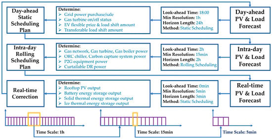
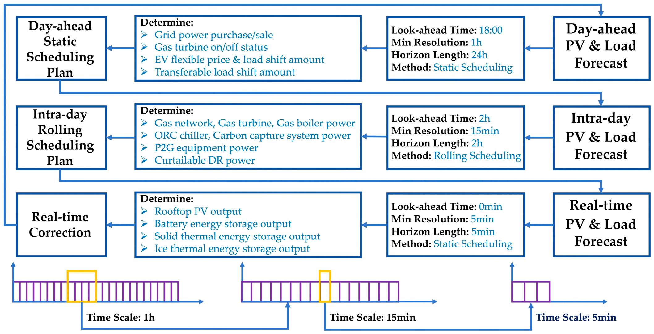
To track source and load uncertainties, this paper adopts an MPC-based three-stage scheduling method comprising day-ahead, intra-day rolling, and real-time correction, as shown in Figure 2. Based on equipment and multi-energy flow balance constraints, this multi-time-scale model determines equipment output by importance and flexibility while leveraging energy storage to smooth fluctuations. Through bidirectional information flow and cascaded constraints, the three layers form an organic whole with a time-based division of labor and step-by-step progression.

Figure 2. Multi-timescale Dispatch Architecture for a Low-Carbon Industrial Park’s Integrated Energy System.

• The day-ahead layer uses a 24 h cycle and 1 h resolution, prioritizing high-importance units. It minimizes total operating cost and introduces the LCT mechanism to internalize carbon emissions into economic cost. Decision variables include main grid power exchange, GT start-stop status, and elastic electricity price response curves of TLs and EVs, providing benchmarks for subsequent layers.
• The intra-day layer adopts a 15 min step size and 2 h rolling window. Retaining key day-ahead variables, it minimizes total operating cost including LCT cost. It further optimizes natural gas supply, GT output, ORC cooling power, and CTCLs, refining macroscopic decisions into executable plans.
• The real-time layer operates at a 5 min resolution. As source-load errors manifest as power fluctuations, the objective switches to minimizing main grid power purchase deviation. This layer utilizes the rapid response capability of the IES, including electricity, heat, and cooling storage, to adjust PV and load changes. It smooths disturbances ensuring real-time stability.

Through layer-by-layer constraint coupling of the three stages, a balanced match between prediction accuracy and response speed is achieved. Minimizing purchased power deviation balances plan and actual matching along with economic efficiency and grid stability. Without subjective weights, the system realizes multi-objective unification of economic drive, low-carbon internalization, and stability correction.

3.2. Basic Principles of Model Predictive Control

The intra-day scheduling layer connects the day-ahead plan and real-time execution with its core being MPC based rolling optimization. To balance foresight and reliability against increasing prediction errors over time, the intra-day stage adopts short-time-window rolling prediction with time varying variance Gaussian noise instead of the coarse-grained day-ahead 24 h curve.

As shown in references [19,20], at each rolling moment t with a 15 min step size where t ranges from 1 to 96, the system forecasts source-load power for the next 2 h, covering eight discrete points corresponding to forecast step k from 1 to 8. This forecast superimposes a zero mean Gaussian forecast error ε onto the day-ahead baseline curve $P_{baseline}$ as shown in Equation (51):

$$\left\{\begin{array}{l}{P}_{\mathit{forecast}}(t,k)=P_{\mathit{baseline}}^k+{\epsilon }_k,\hspace{1em}{\epsilon }_k~\mathcal{N}(0,{\sigma }_k^2)\hfill \\ {\sigma }_k={\sigma }_0+\Delta \sigma \cdot (k-1),\hspace{1em}k=1,2,\dots ,8\hfill \end{array}\right.$$

(51)

where ${\sigma }_0$ is the minimum standard deviation for the next 15 min, and Δσ > 0 is the increment step that ensures ${\sigma }_k$ strictly increases with k. This time-varying variance reflects the physical principle that longer forecast horizons yield higher uncertainty, meaning that the first point has the highest confidence and the eighth has the lowest. Different baseline standard deviations are applied to PV, heat, cooling, electricity, and gas loads, but the increasing logic remains consistent, reflecting the decay in confidence.

The forecast curves are directly transformed into constraint boundaries. Source-side forecast values serve as inequality upper bounds that limit dispatchable resources, while load-side values serve as right-hand side terms in equations that enforce strict supply–demand balance. This gives rise to a dynamically shrinking feasible solution space within the eight-point look-ahead window.

Following previous research [21,22,23], after generating the forecast, the optimizer solves a global economic optimization problem covering the next eight time steps, and the resulting open-loop control sequence is expressed as Equation (52):

$$u_t^{*}={\left[\begin{array}{c}{u}_{t,0}^{*},u_{t,1}^{*},\dots ,u_{t,7}^{*}\end{array}\right]}^T$$

(52)

where $u_{t,k}^{\ast }$ is the control decision made at rolling moment t for the k-th step prediction.

However, only the first control action in this sequence is actually issued for execution, as shown in Equation (53):

$$u_{\mathit{actual}}(t)=u_{t,0}^{*}$$

(53)

The remaining seven values are discarded. This eight-step prediction and one-step execution strategy has a twofold rationale. First, the extended horizon prevents single-step greedy decisions causing instability, allowing the optimizer to assess future impacts and yield a globally superior trajectory. Second, since the eighth point has larger variance than the first, dispatching low reliability actions causes irreversible cumulative deviations. Thus, only the shortest step command is applied.

When time advances to moment t + 1, the system executes the feedback loop by updating state variables and locking previous control actions as equality constraints. All past decision variables are fixed to historical actual values, as shown in Equation (54):

$$u_{\mathit{opt}}(\tau )=u_{\mathit{hist}}(\tau ),\hspace{1em}\forall \tau \le t$$

(54)

where $u_{opt}$ is the decision variable and $u_{hist}$ is the actual executed control action determined by feedback or a prior plan. This locking transforms historical variables into known constants eliminating open loop error propagation. The system then regenerates an eight-step prediction sequence with variance increasing again from ${\sigma }_0$ and solves the optimization problem once more. This coupled cycle of time-varying variance-prediction long-horizon look-ahead single-step execution and historical locking transforms the stochastic optimization problem with long-period coupling constraints into a series of local quasi-steady MILP problems with deterministic boundaries, ensuring solution feasibility and practicality.

Unlike the intra-day rolling mechanism, the real-time scheduling layer does not rely on iterative forecasting. Its source-load curve generation adopts a one-time global expansion with a constant variance pattern, as shown in Equation (55). Operating at a 5 min granularity, this stage covers 288 dispatch points. The real-time layer retrieves the 96 baseline values from the intra-day stage, expands them into a 288 dimensional vector, and independently superimposes Gaussian noise with fixed standard deviation at each time step:

$$P_{\mathit{real}}(i)=P_{\mathit{intra}}(i)\cdot (1+{\xi }_i),\hspace{1em}{\xi }_i~\mathcal{N}(0,{0.05}^2),\hspace{1em}i=1,2,\dots ,288$$

(55)

where $P_{intra}$ is the planned power at the i-th 5 min point interpolated from intra-day baselines. The standard deviation is constant because the extremely short advance time makes forecast errors insensitive, acting as a steady state disturbance. Since the goal is minimizing power deviation rather than economic optimality, no look-ahead window is needed. It uses energy storage to smooth minor fluctuations in one pass. Based on the latest intra-day plan, it solves the 288-dimensional deviation minimization problem once and outputs real-time commands.

Although using Gaussian random numbers real-time generation lacks time-varying variance and rolling discarding, differing from the intra-day stage, this stems from distinct timescales and objectives. The intra-day stage balances economy and operation time while the real-time stage focuses on precise automated response. These mechanisms complement each other, forming a complete closed loop of stepwise refinement in multi-timescale scheduling.

3.3. Scheduling Objective Function and Constraints

Day-ahead scheduling usually takes place at 18:00 the day before, with the purpose of pre-establishing an economically stable day-ahead scheduling plan based on the forecast of distributed generation output curves, electricity-heat-cooling loads, EV loads, and outdoor temperature for the next 24 h. This plan fully utilizes transferable loads and the DR of elastic electricity prices to achieve peak shaving and valley filling, and prioritizes the determination of operation parameters for units with the highest importance level or the greatest scheduling difficulty.

The economic operation cost of the IES mainly includes the interaction cost with energy networks, the operation and maintenance (O&M) cost of internal equipment, and the DR cost. The total operating cost function of the day-ahead scheduling is shown in Equation (56):

$$\begin{array}{ll}\hfill W_{\mathit{dayahead}}& =W^{PV}+W^{GT}+W^{\mathit{GB}}+W^{\mathit{ORC}}+W^{\mathit{EGrid}}+W^{\mathit{GGrid}}+W^{\mathit{CE}}\hfill \\ & +W^{\mathit{BES}}+W^{\mathit{STES}}+W^{\mathit{ITES}}+W^F+W^{\mathit{TL}}+W^{\mathit{CC}}+W^{P2G}\hfill \end{array}$$

(56)

where $W_{dayahead}$ is the total operating cost; $W^{PV}$ is the PV system operating cost; $W^{GT}$ is the GT operating cost; $W^{GB}$ is the GB operating cost; $W^{ORC}$ is the ORC waste heat chiller operating cost; $W^{EGrid}$ is the grid power exchange cost; $W^{GGrid}$ is the gas purchase cost; $W^{CE}$ is the LCT cost; $W^{BES}$, $W^{STES}$, and $W^{ITES}$ are the storage system depreciation costs; $W^F$ is the CTCL DR compensation cost; $W^{TL}$ is the TL DR compensation cost; $W^{CC}$ is the CCS operating cost; and $W^{P2G}$ is the P2G operating cost.

Day-ahead constraints encompass device operational characteristics, source-load multi-energy flow balance, and indoor temperature constraints. These include GT heat power coupling, PV efficiency, ORC conversion, GB gas heat conversion, CTCL comfort, IES power capacity coupling, and multi-energy flow balance. Device constraints are expressed as Equations (1)–(20) and (27)–(46) while power balance and temperature constraints are given in Equations (47)–(50) and (57):

$$\left\{\begin{array}{l}{H}_t^F=H_t^{\mathit{Fset}}\hfill \\ L_t^F=L_t^{\mathit{Fset}}\hfill \end{array}\right.$$

(57)

where $H_t^F$ and $L_t^F$ are the actual heating and cooling power of the CTCL, and $H_t^{Fset}$ and $L_t^{Fset}$ are the setpoints. Solving the day-ahead optimization preferentially determines key parameters, including grid power exchange, GT on–off status, elastic electricity price, and DR power profiles for EVs and TLs.

In the intra-day stage, parameters such as PV generation, PV thermal power, electric, thermal, cooling, and natural gas loads, uncoordinated EVs, uncoordinated TLs, and outdoor temperature are predicted again. To address significant day-ahead prediction errors, the intra-day stage shortens the forecast lead time to 2 h. The temporal resolution is also refined to 15 min. MPC is then adopted for rolling prediction and scheduling to improve the economic dispatch. The intra-day objective function matches the day-ahead one, as shown in Equation (56). Because it uses higher-precision data, this stage provides results closer to actual conditions.

Intra-day constraints comprise four components: individual equipment operating constraints in Equations (1)–(20) and (27)–(46), source-load multi-energy flow balance constraints in Equations (47)–(50), day-ahead and intra-day coupling constraints in Equation (58), and temporal coupling constraints between successive intervals in Equation (59). Day-ahead and intra-day coupling ensures adherence to key day-ahead variables, such as grid power exchange, GT status, EV electricity price, and DR amount. Meanwhile, temporal coupling guarantees equipment state continuity.

$$\left\{\begin{array}{l}{E}_t^{\mathit{buy}}=E_{t,\mathit{dayahead}}^{\mathit{buy}}\hfill \\ E_t^{\mathit{sell}}=E_{t,\mathit{dayahead}}^{\mathit{sell}}\hfill \\ U_t^{GT}=U_{t,\mathit{dayahead}}^{GT}\hfill \\ P_t^{\mathit{EV}}=P_{t,\mathit{dayahead}}^{\mathit{EV}}\hfill \\ \Delta E_t^{\mathit{EV}}=\Delta E_{t,\mathit{dayahead}}^{\mathit{EV}}\hfill \\ \Delta E_t^{\mathit{TL}}=\Delta E_{t,\mathit{dayahead}}^{\mathit{TL}}\hfill \end{array}\right.$$

(58)

$$\left\{\begin{array}{l}{E}_{t-1}^{GT}=E_{t-1,\mathit{intraday}}^{GT}\hfill \\ H_{t-1}^{GT}=H_{t-1,\mathit{intraday}}^{GT}\hfill \\ H_{t-1}^{\mathit{GB}}=H_{t-1,\mathit{intraday}}^{\mathit{GB}}\hfill \\ L_{t-1}^{\mathit{ORC}}=L_{t-1,\mathit{intraday}}^{\mathit{ORC}}\hfill \\ L_{t-1}^{\mathit{EL}}=L_{t-1,\mathit{intraday}}^{\mathit{EL}}\hfill \\ H_{t-1}^{\mathit{EH}}=H_{t-1,\mathit{intraday}}^{\mathit{EH}}\hfill \\ G_{t-1}^{\mathit{buy}}=G_{t-1,\mathit{intraday}}^{\mathit{buy}}\hfill \end{array}\right.$$

(59)

The core idea of intra-day rolling scheduling is as follows. At time t, ultra-short-term source-load forecasts for intervals t + 1 to t + 8, covering a 2 h horizon, day-ahead parameters, and previous intra-day states are taken as inputs and substituted into Equations (1)–(20), (27)–(50), (56), (58) and (59) for optimization. Only the control action for time t + 1 is implemented. This rolling process repeats until all 96 time slots are scheduled. Intra-day scheduling further determines the variables of equipment with higher importance and lower flexibility, including GT power generation and heat output, GB heat output, ORC cooling power, CTCL DR amount, CAC cooling and heating power, and gas purchase power.

Real-time scheduling optimization uses a 5 min resolution. The control side responds autonomously without scheduling commands to achieve efficiency and stability. After day-ahead and intra-day scheduling, the system operating cost is minimized, leaving limited rescheduling capacity. Real-time scheduling mainly relies on the fastest responding ESS to correct deviations. Its objective minimizes the main grid interaction power deviation relative to the intra-day plan with the objective function given in Equation (60):

$$\min S^{\mathit{realtime}}={\displaystyle \sum _{t=1}^T\left|(E_{t,\mathit{realtime}}^{\mathit{buy}}-E_{t,\mathit{realtime}}^{\mathit{sell}})-(E_{t,\mathit{intraday}}^{\mathit{buy}}-E_{t,\mathit{intraday}}^{\mathit{sell}})\right|}$$

(60)

where $S^{realtime}$ is the absolute deviation of main grid power exchange between real-time and intra-day scheduling. Smaller deviations indicate better correction and reduce the impact of PV and load fluctuations on the upper grid.

Real-time constraints also consist of four parts: equipment operation, multi-energy flow balance, real-time and day-ahead coupling, and real-time and intra-day coupling. The real-time and day-ahead coupling removes the grid power purchase assignment from Equation (58), while the real-time and intra-day coupling ensures fine adjustments based on intra-day equipment outputs, as shown in Equation (61):

$$\left\{\begin{array}{l}{E}_t^{\mathit{CHP}}=E_{t,\mathit{intraday}}^{\mathit{CHP}}\hfill \\ H_t^{\mathit{CHP}}=H_{t,\mathit{intraday}}^{\mathit{CHP}}\hfill \\ H_t^{\mathit{GB}}=H_{t,\mathit{intraday}}^{\mathit{GB}}\hfill \\ L_t^{\mathit{ORC}}=L_{t,\mathit{intraday}}^{\mathit{ORC}}\hfill \\ L_t^{\mathit{EL}}=L_{t,\mathit{intraday}}^{\mathit{EL}}\hfill \\ H_t^{\mathit{EH}}=H_{t,\mathit{intraday}}^{\mathit{EH}}\hfill \\ G_t^{\mathit{buy}}=G_{t,\mathit{intraday}}^{\mathit{buy}}\hfill \end{array}\right.$$

(61)

Real-time scheduling finally determines variables for lower importance and highest flexibility equipment including rooftop PV output, BES charging, and discharging power STES heat power and ITES cooling power. In summary, the multi-timescale scheduling model successively determines equipment outputs by importance and flexibility, fully exploiting flexible energy storage to minimize grid power purchase deviation between day-ahead and real-time stages. It effectively balances conflicts between prediction errors and preparation time, pre-scheduled plans and actual implementation, and economic efficiency and grid stability.

4. Case Study and Result Verification

Taking a typical summer day of an IES in a low-carbon park managed by State Grid Shandong Electric Power Co., Ltd. as an example, the model data, which combine the actual project parameters with the reference data from [12,13,21], are presented as follows. The equipment operating parameters are listed in Table 2; the natural gas price is CNY 3.5/m³; and the TOU electricity price and the EV flexible electricity price coefficient matrix are detailed in Table 3 and Table 4, respectively.

Table 2. Main operating parameters of major IES equipment.

Unit	Parameter	Value	Unit	Parameter	Value	Unit	Parameter	Value
PV	$S^{PVE}$(m2)	2250	GT	$H_{max}^{GT}$(kW)	400	Grid	$E_{max}^{Grid}$(kW)	2000
	$S^{PVH}$(m2)	200		$H_{min}^{GT}$(kW)	0		$G_{max}^{Grid}$(m3/h)	100
	${\eta }_E^{PV}$(%)	17.5%		$E_{max}^{GT}$(kW)	380	BES	$S_{max}^{BES}$(kWh)	2000
	${\eta }_H^{PV}$(%)	35%		$E_{min}^{GT}$(kW)	100		$S_{min}^{BES}$(kWh)	400
	$E_N^{PV}$(kW)	200		$E_0^{GT}$(kW)	180		$S_0^{BES}$(kWh)	1000
	$H_N^{PV}$(kW)	50		$k_{up}$(/)	−0.45		$E_{max}^{BESC}$(kW)	200
	$E_u^{PV}$(W/m2)	100		$k_{dn}$(/)	0.75		$E_{max}^{BESD}$(kW)	200
	$H_u^{PV}$(W/m2)	250		${\eta }_e^{GT}$(/)	0.4	STES	$S_{max}^{STES}$(kWh)	1500
LCT	γ (/)	1.37		$p_n^{GT}$(CNY/time)	80		$S_{min}^{STES}$(kWh)	400
	d (ton)	3.75		$p_{off}^{GT}$(CNY/time)	80		$S_0^{STES}$(kWh)	600
	K (/)	5		$p_e^{GT}$(CNY/kWh)	0.07		$H_{max}^{STESC}$(kW)	200
	$c_0$(CNY/t)	75		$p_h^{GT}$(CNY/kWh)	0.07		$H_{max}^{STESD}$(kW)	150
ORC	${\eta }_L^{ORC}$(/)	0.295	Natural Gas	$Q_{gas}$(J/m3)	3.60 × 107	ITES	$S_{max}^{ITES}$(kWh)	2000
	$p^{ORC}$(CNY/kWh)	0.07		${\xi }_{gas}$(kg/m3)	1.89		$S_{min}^{ITES}$(kWh)	400
GB	${\eta }^{GB}$(/)	0.83		$p^{Gbuy}$(CNY/m3)	3.5		$S_0^{ITES}$(kWh)	600
Others	${\zeta }^{TL}$(CNY/kWh)	15	Others	$F_t^{set}$(°C)	25		$L_{max}^{ITESC}$(kW)	200
	${\xi }^F$(CNY/kWh)	0.35					$L_{max}^{ITESD}$(kW)	200

Table 3. Time-of-Use Electricity Rates.

Time Period	Period Type	Price (CNY/kWh)
00:00–06:00	Valley	0.32
6:00–11:00	Peak	1.15
11:00–17:00	Flat	0.61
17:00–22:00	Peak	1.15
22:00–24:00	Valley	0.32

Table 4. Electric vehicle price elasticity coefficient matrix.

Time Period	Valley	Flat	Peak
Valley	−0.15	0.011	0.013
Flat	0.011	−0.15	0.018
Peak	0.013	0.018	−0.15

The proposed multi-timescale model incorporates nonlinear features arising from GT electro-thermal coupling, ESS charge-discharge transitions, CAC mode exclusivity, CCS and P2G efficiencies, LCT piecewise functions, and TL peak-shaping mechanisms. To improve computational efficiency, piecewise linearization is applied to convert these nonlinear relationships into linear constraints. Additionally, binary variables are introduced to characterize equipment status and operational choices. The linear model was solved via YALMIP R20180817 and Gurobi 9.0.2 in MATLAB R2018b on an Intel i7 with 16 GB RAM. The Gurobi solver achieved an optimal gap of 0.01% across all three scheduling stages. Results show that the day-ahead optimization took 18.5 s in total, the intra-day rolling at 15 min steps averaged 2.8 s per step with a maximum of 4.1 s, and the real-time correction at 5 min intervals averaged 0.35 s per interval, confirming its suitability for online applications.

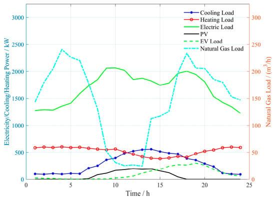
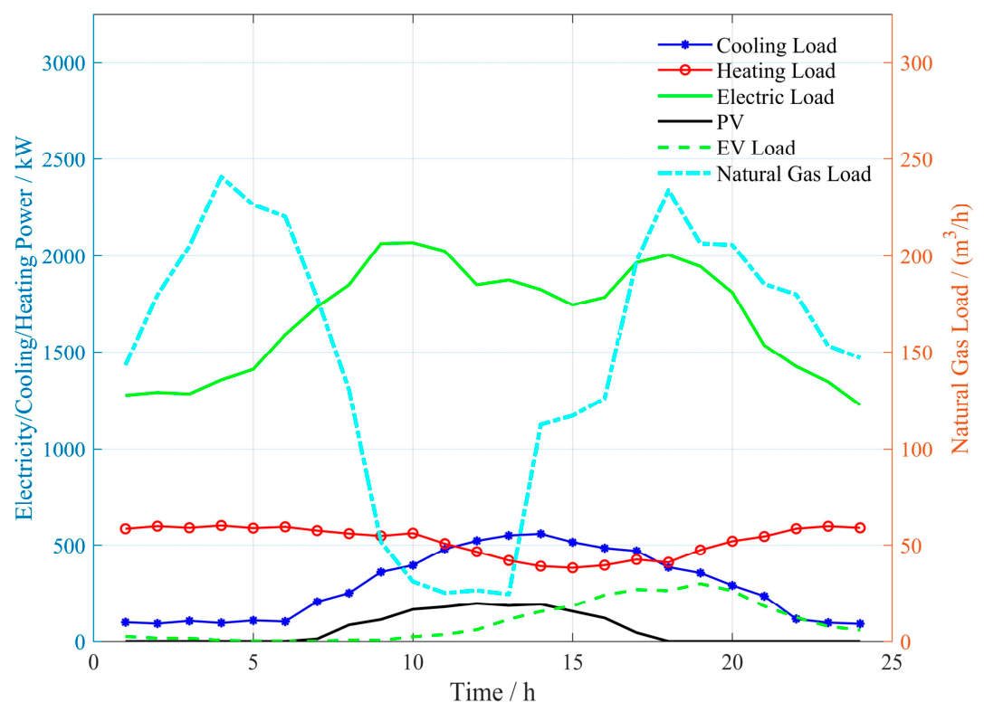
Figure 3 illustrates typical daily multi-energy flow curves based on previously published data [21,22,23]. PV electric output is concentrated between 06:00 and 17:00, peaking at 196.7 kW at 11:00. PV thermal output follows a similar trend, peaking at approximately 49.5 kW at 10:00. The electric load exhibits double-peak characteristics, peaking at 09:00, reaching approximately 2068.8 kW, and at 18:00, reaching about 2005 kW. The cooling load peaks in the afternoon at 558.5 kW at 13:00. The heating load shows a U-shaped variation, dropping to a minimum of 382.0 kW in the afternoon from 585–602 kW at night. Natural gas load has morning and evening peaks at 03:00, approximately 240.9 kW, and 17:00, about 234.1 kW. Uncoordinated EV charging is concentrated from afternoon to evening, peaking at 299.0 kW at 18:00. These complex, coupled source-load characteristics with interleaving peaks and valleys pose challenges that single-timescale methods struggle to address.

Figure 3. Day-ahead forecasted multi-energy flow stochastic source-load curves.

4.1. Day-Ahead Scheduling Simulation Results and Analysis

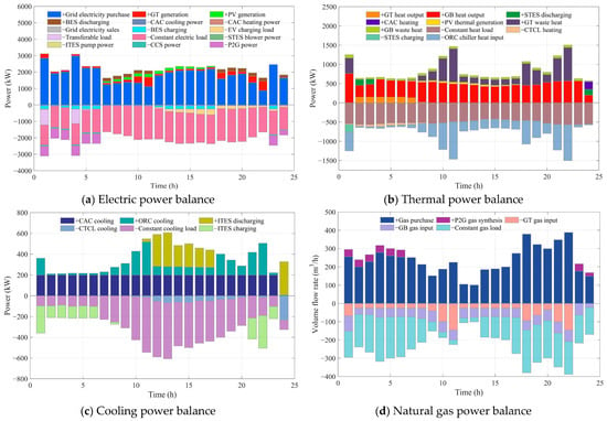
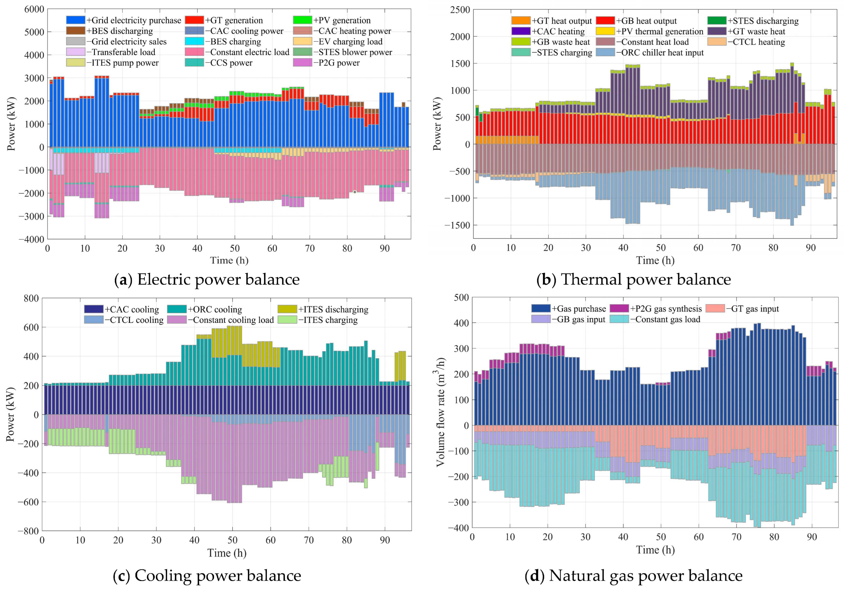
As shown in Figure 4a, in the day-ahead stage, the simulated low-carbon park IES shows strong grid dependence and multi-energy regulation. Purchased electricity totals 49,155 kWh, accounting for 86.6% of supply, with high off-peak levels of 1900 to 2984 kW indicating limited energy storage shifting. The GT generates 4576 kWh, peaking at 580 kW at 11:00 and 22:00, and shutting down at night to reflect economic dispatch. PV contributes 1425 kWh, peaking at 190 kW at 12:00. The battery charges from 1:00 to 6:00 and 13:00 to 17:00, and discharges during peak price periods. However, a net charge of 1392 kWh shows that the battery does not fully release its energy due to SOC limits.

Figure 4. Results of multi-energy flow optimization for day-ahead scheduling: (a) Electric power balance; (b) Thermal power balance; (c) Cooling power balance; (d) Natural gas power balance.

At the DR level, price signals reshape load patterns. EV charging shifts to flat price periods but retains 119 to 196 kW during the evening peak, indicating incomplete peak avoidance. The TL shows a leapfrog concentration activated only in the early morning, reflecting the coarse-grained nature of day-ahead dispatch.

As shown in Figure 4b,c, heating and cooling dispatch demonstrate effective waste heat utilization and multi-source supply. The GB provided 12,032 kWh, or 88% of total heat, operating continuously. The GT provided only 732 kWh. GT waste heat drove the ORC chiller for cooling, with heat consumption peaking at 971 kW at 11:00. The CAC served as a base source at 200 kW. The ORC chiller provided 2432 kWh, reducing electric cooling reliance. The ITES shifted cooling load by charging at night and discharging from noon to evening, peaking at 327 kW.

According to Figure 4d, the system purchased 5978 m³ of natural gas, with the GT and GB consuming 1063 m³ and 1306 m³. Purchased gas peaked during 18:00 to 22:00. P2G operated during nighttime valley hours to produce methane with CCS, reducing net emissions. Total emissions were 4.46 tons, dropping to 3.89 tons after P2G absorption, a 13% reduction highlighting the role of P2G.

Overall, day-ahead scheduling achieved balance via TOU pricing, waste heat transfer, ice storage, and DR. However, high levels of purchased electricity, incomplete battery cycling, discrete TL, and concentrated EV peaks show limitations in coping with uncertainty. The system remained rigidly grid-dependent. This indicates the need for intra-day and real-time adjustments to reduce grid fluctuations, improve waste heat use, and enhance precision.

4.2. Intra-Day Scheduling Simulation Results and Analysis

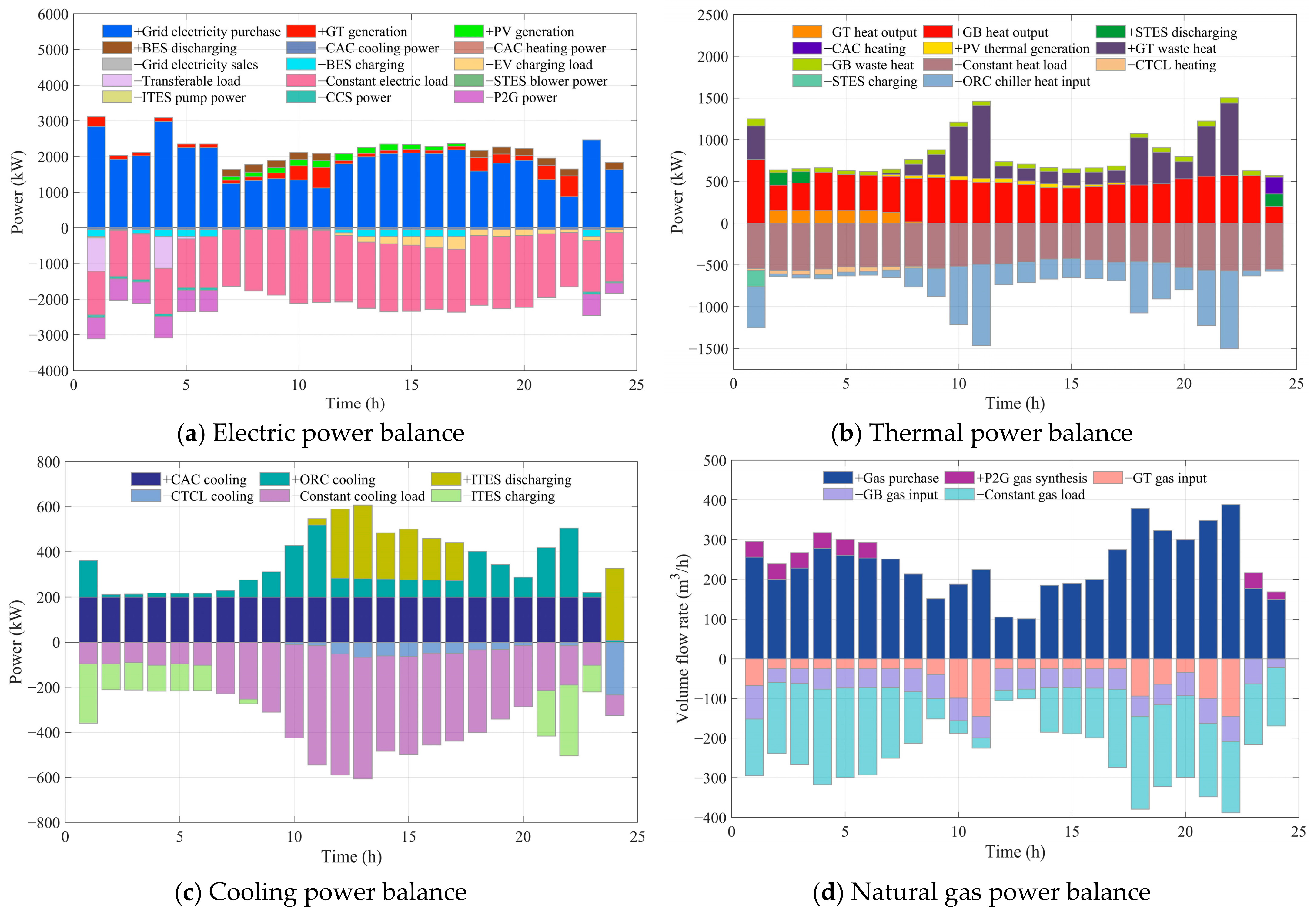
The intra-day scheduling stage operates on a 15 min timescale built upon the day-ahead framework and stochastic rolling prediction. It is designed to perform adaptive calibration and refined adjustment through accurate short-term prediction curves. From the perspective of the overall supply–demand structure, while maintaining the main equipment framework, intra-day scheduling significantly enhances dispatch efficiency and self-balancing capability. Figure 5a shows that the total purchased electricity decreased by 5.60% compared with day-ahead scheduling, with the proportion of purchased electricity at 82.12%. This indicates that intra-day scheduling effectively activates distributed flexible resources, moderately reducing dependence on the main grid while maintaining macro-level stability for more economical and efficient energy allocation. For units with greater scheduling difficulty, the 15 min rolling optimization achieved deep refinement. The GT unit power generation increased significantly by 40.70%, accurately filling intra-day power deficits through frequent ramping responses. As illustrated in Figure 5d, P2G and CCS make full use of surplus electricity during valley periods and PV surpluses, with their electricity consumption increasing by 12.69% and 22.32%. The ITES breaks through the day-ahead single charge-discharge mode, exhibiting a nested multi-period strategy with efficiency maintained at 74.8%, demonstrating that short-timescale scheduling expands operational boundaries of complex energy storage units.

Figure 5. Results of multi-energy flow optimization for intra-day scheduling: (a) Electric power balance; (b) Thermal power balance; (c) Cooling power balance; (d) Natural gas power balance.

Figure 5b,c illustrate the operational reliability of intra-day scheduling, which demonstrates a multi-energy flexible support mechanism. Faced with a surge in temperature-controlled cooling load of 16.84% and heating fluctuations, the system relies on deep coupling. Specifically, the system instantly switches ITES states for high-frequency load shifting while ramping up GT output. This releases abundant waste heat, driving the ORC chiller with heat consumption increasing by 41.12%, effectively resolving sudden cooling demand. This synergy ensures supply reliability for high-priority loads under extreme fluctuations.

In summary, the intra-day scheduling mechanism based on a 15-min interval effectively bridges the deviation between the day-ahead plan and actual operation. It optimizes the overall energy flow structure and achieves flexible dispatch of slow rigid units, demonstrating the flexible mutual support advantage and excellent self-balancing capability of the IES under high-frequency fluctuations.

4.3. Real-Time Scheduling Simulation Results and Analysis

The real-time stage operates at 5 min intervals, leveraging the electricity-heating–cooling system to buffer source-load fluctuations. According to Equation (55), under zero-mean stochastic errors, cumulative deviations tend to cancel over the 24 h horizon, substantially lowering the storage demand for smoothing. Simulation results confirm that real-time deviations for electricity, heating, and cooling are maintained at 0.17%, 0.10%, and 0.06%, respectively, demonstrating accurate intra-day plan tracking and effective fluctuation mitigation through multi-energy coordination.

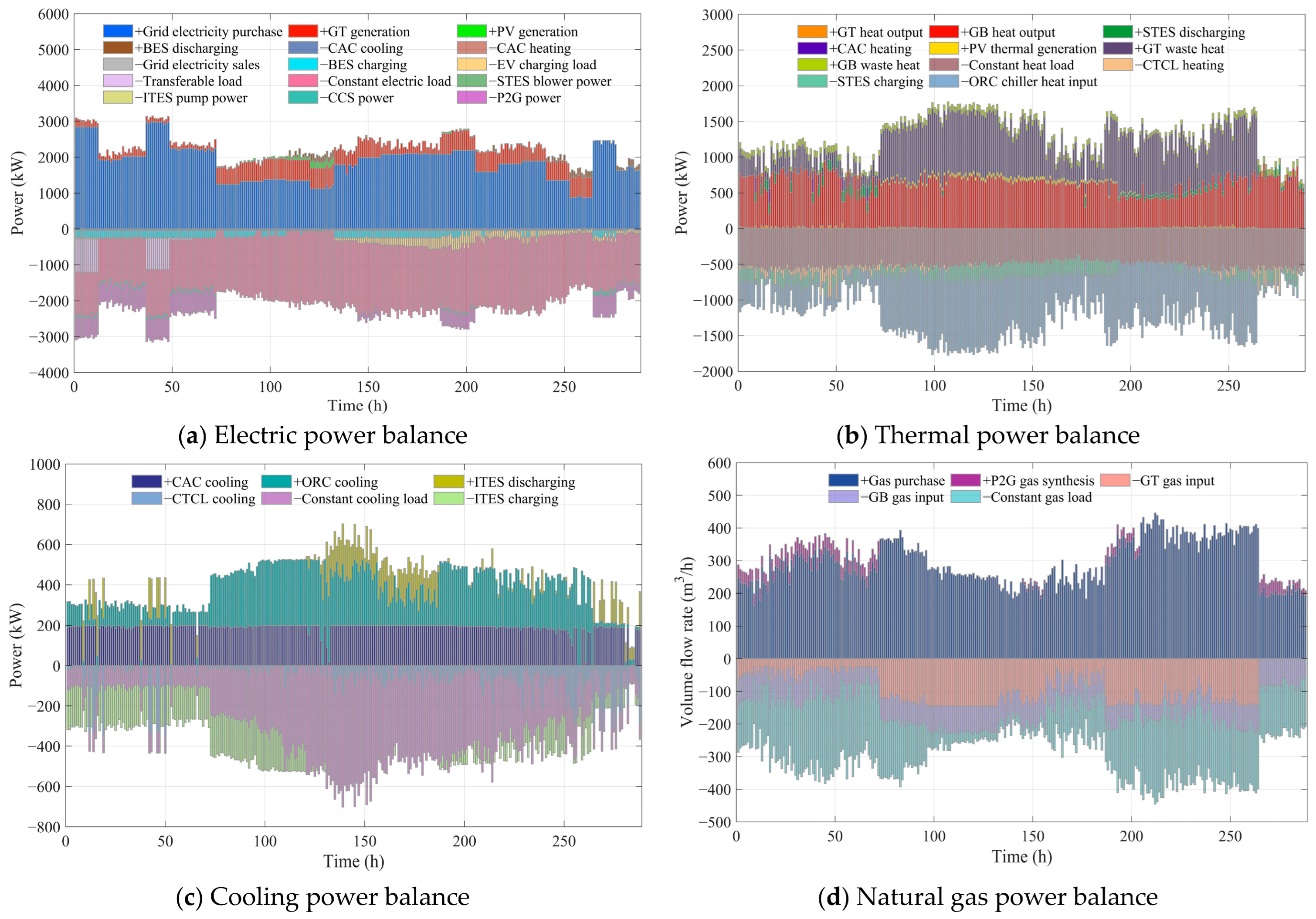
As detailed in Figure 6a,d, in the evolution of the multi-energy flow, the equipment exhibits flexible shifting and precise start-stop characteristics. Guided by real-time signals, the CAC shifts output to periods of flat electricity pricing, performing high-frequency adaptive switching within the 0 to 200 kW range. In contrast, the P2G equipment shows concentrated dispatch characteristics with valley filling and pulse absorption, activated only during specific times such as 0:00 to 6:00 and 16:00 to 17:00, with zero output otherwise.

Figure 6. Results of multi-energy flow optimization for real-time scheduling: (a) Electric power balance; (b) Thermal power balance; (c) Cooling power balance; (d) Natural gas power balance.

The high-frequency pulse characteristics of the IES at a 5 min resolution are key to reducing energy storage demand. According to Figure 6b,c, both STES and ITES discharge follow a multi-pulse, short-duration response pattern. Within multiple 5 min windows, the STES is instantaneously activated at 150 kW and the ITES at 200 kW, precisely offsetting instantaneous fluctuations of TCLs. Furthermore, the deep integration of heat-power decoupling allows waste heat cooling driven by the ORC to account for 43.99% of the total, nearly matching the 45.67% share of electric cooling. By effectively utilizing GT waste heat as a buffer, the thermal system transforms into a flexible resource for absorbing power fluctuations. In summary, the 5 min scheduling strategy achieves rapid hedging of source-load variations through coordinated IESS smoothing and multi-energy coupling, ensuring high-precision supply–demand matching and reducing the need for large-scale energy storage.

4.4. Comparative Analysis of Electricity-to-Gas Conversion and Demand Response

Figure 4, Figure 5 and Figure 6 illustrate the electric, heating, cooling, and gas power balances across the day-ahead, intra-day, and real-time stages. The real-time stage primarily minimizes power deviations with the distribution network to ensure high-precision tracking of the intra-day plan and enhance grid stability. However, because its objective function excludes economic and carbon trading costs, it cannot directly evaluate the energy-saving and emission-reduction benefits of DR and P2G. In contrast, the intra-day rolling stage inherits day-ahead DR and P2G decisions, handles stochastic fluctuations, and retains total operating and carbon costs. Notably, DR and P2G serve complementary but distinct roles within the proposed framework; DR primarily drives economic optimization by reshaping load profiles through TOU pricing, while P2G (coupled with CCS) primarily enables low-carbon transformation by converting captured CO₂ into synthetic methane. Therefore, subsequent comparative analyses of scenarios with and without DR or P2G are based on intra-day results to accurately reflect their comprehensive value under uncertain source load.

4.4.1. Comprehensive Analysis of the Benefits of Demand Response

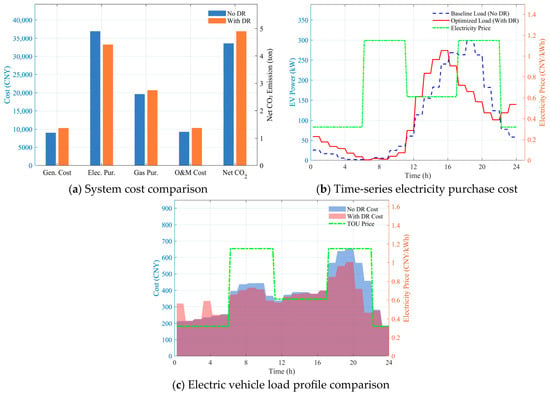
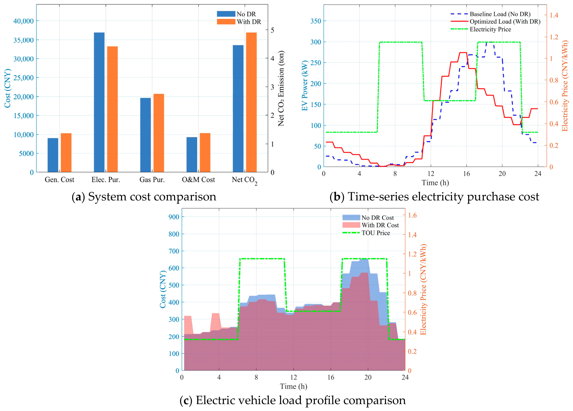
As shown in Figure 7a and Table 5, implementing the TOU-based DR strategy increases power generation, gas procurement, and O&M costs by 14.29%, 5.76%, and 11.41%, respectively. However, electricity procurement costs decrease significantly, by 9.97%. This reduction fully offsets the increases in other costs, thereby lowering the overall energy cost. This reflects a strategic gas-for-electricity substitution; under DR regulation, the system replaces expensive peak-hour grid purchases with local gas-fired generation, trading relatively controllable gas and O&M expenses for greater electricity savings. Carbon emissions increased from 4.4624 tons to 4.909 tons, representing a 10% increase. This serves as a reasonable physical cost for the system to pursue economic optimality in a market environment without strong carbon constraints.

Figure 7. Comparative analysis of demand response benefits: (a) System cost comparison; (b) Time-series electricity purchase cost; (c) Electric vehicle load profile comparison.

Table 5. Comparison of system costs with and without demand response.

Item	No DR	With DR
Generation cost (CNY)	9026.39	10,316.44
Electricity purchase cost (CNY)	36,964.90	33,280.03
Gas purchase cost (CNY)	19,645.90	20,776.72
O&M cost (CNY)	9287.17	10,346.58
Net carbon emissions (ton)	4.462	4.909

As detailed in Figure 7b, the temporal distribution of electricity purchase costs reflects the response capability of DR to price signals. During the high-price peak interval, DR exhibits a stronger hedging mechanism, significantly reducing single-period costs compared to the scenario without DR. During the electricity price valley interval, DR actively increases electricity consumption to absorb shifted loads, resulting in higher costs than the non-DR scenario. During the flat-price period, costs remain close, reflecting that the DR algorithm concentrates dispatch resources on peak–valley price spread arbitrage.

Figure 7c illustrates the optimization results of the EV load verify the capability of DR to reshape load distribution. Under the uncoordinated charging scenario, the concentrated evening peak load was 299.13 kW. DR reduced the optimized load peak to 274.24 kW, achieving a peak shaving of 8.32%. These curtailed loads during high-price periods shifted to the nighttime valley period. Total electricity consumption remained constant. Through spatiotemporal load shifting aligned with TOU pricing, DR reduced the actual EV electricity purchase cost from CNY 2072.29 to CNY 1761.44, achieving a 15% reduction and demonstrating its critical role in lowering user energy costs.

4.4.2. Comprehensive Analysis of the Benefits of Electricity-to-Gas Conversion

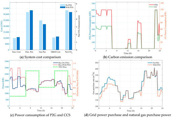
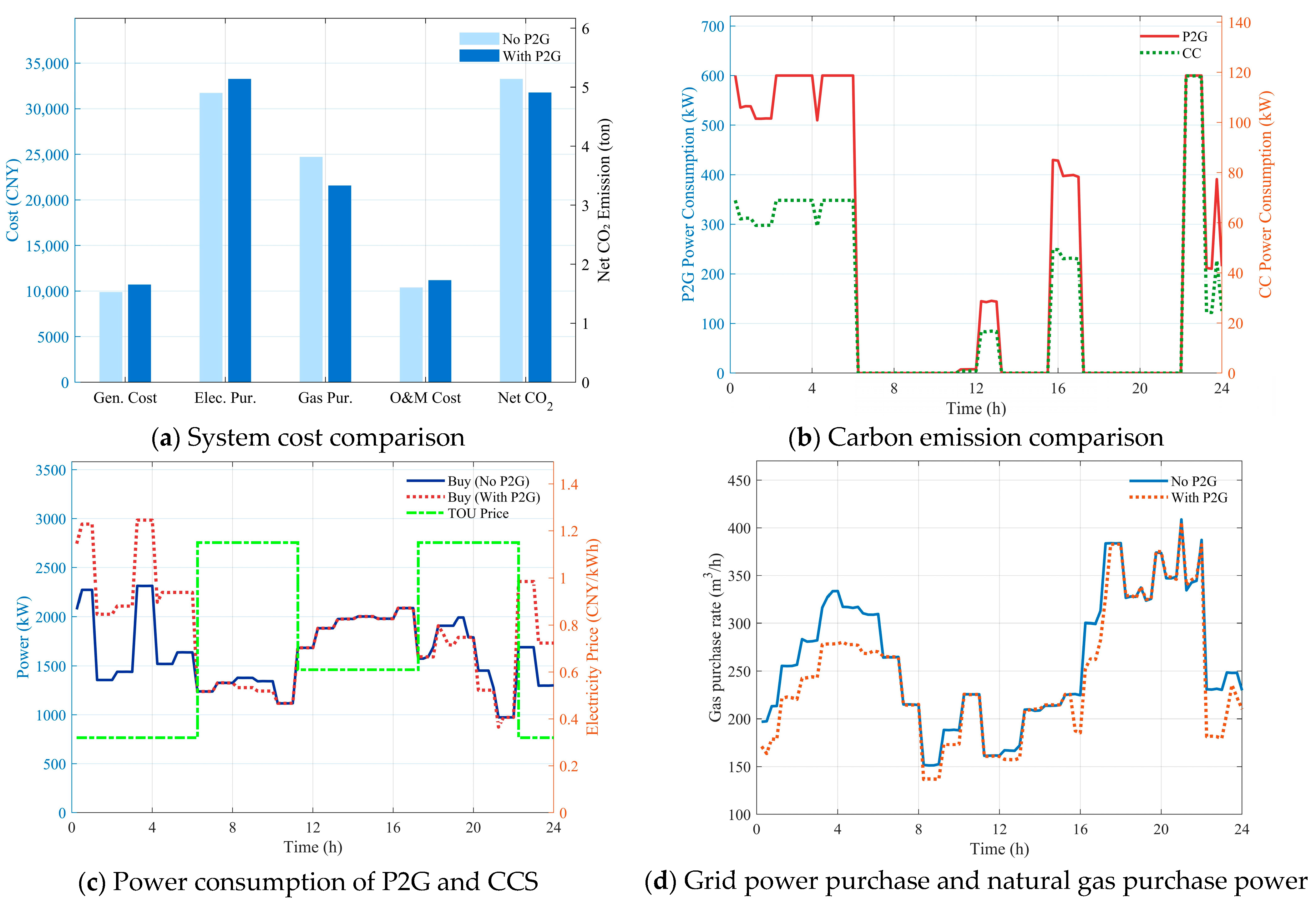
As shown in Figure 8a and Table 6, after introducing P2G, the system achieves cross-energy cost transfer. Generation and electricity purchase costs increase by 8.30% and 4.87%, respectively, reflecting a strategy of substituting electricity for gas. By increasing electricity consumption, gas purchase costs drop significantly by 12.70%. The savings in gas costs cover the rise in electricity costs, thereby reducing total system costs. O&M costs increase by 7.72%, representing a necessary investment to ensure the efficient operation of P2G and CCS, supporting multi-energy coupling functions. Regarding carbon emissions, net emissions decrease from 5.14 tons to 4.91 tons. This indicates that P2G acts as an efficient chemical carbon sink, converting CO₂ facing high-tier penalties into methane to offset gas consumption, exchanging a marginal increase in operating costs for valuable carbon penalty savings.

Figure 8. Comparative analysis of power-to-gas integration benefits: (a) System cost comparison; (b) Carbon emission comparison; (c) Power consumption of P2G and CCS; (d) Grid power purchase and natural gas purchase power.

Table 6. Comparison of system costs with and without power-to-gas.

Item	No P2G	With P2G
Generation cost (CNY)	9895.03	10,716.44
Electricity purchase cost (CNY)	31,735.22	33,280.03
Gas purchase cost (CNY)	24,714.88	21,576.72
O&M cost (CNY)	10,393.91	11,196.58
Net carbon emissions (ton)	5.140	4.909

As detailed in Figure 8b,c, the power consumption time series of P2G and CCS demonstrates a rapid response to TOU pricing signals. P2G exhibits a strong preference for low prices, maintaining full-power operation at 600 kW during valley periods of 0:00 to 6:00 and 22:00 to 24:00 at CNY 0.32/kWh, while completely shutting down during peak periods at 1.15 yuan/kWh. This concentrated output strategy indicates accurate economic dispatch logic. It coordinates with CCS through simultaneous start-up and shutdown, allowing chemical conversion and physical capture to operate in parallel for optimal cost-effectiveness. Grid purchase data confirms the positive role of P2G in absorbing low-price electricity. Total purchased electricity increases by 11.3% to 43,782.59 kWh, with peak power rising to 2985.13 kW. These increments are concentrated during nighttime valley periods, showing that P2G absorbs large amounts of low-price surplus power. This pattern achieves an excellent peak-shaving and valley-filling effect, improving the grid load factor.

Figure 8d reveals that P2G achieves import substitution. Total daily gas purchase drops by nearly 13% to 6164.78 m³. During nighttime valley periods when P2G operates at full power, pipeline gas purchases are effectively suppressed. This shows the system uses low-price electricity for self-production, shifting energy procurement from external high-price networks to efficient internal production. This reduces dependence on external gas sources, lowers total gas costs, and enhances the energy self-sufficiency rate and operational security of the IES.

5. Conclusions and Future Prospects

Addressing the operational challenges of low-carbon park IES under dual source-load uncertainties and multi-timescale decision conflicts, this paper constructs a multi-time-scale optimal scheduling model based on DR and multi-energy flow coupling. The model adopts a day-ahead, intra-day, and real-time progressive optimization framework, integrating the LCT mechanism, P2G, and multiple flexible load response strategies. Through hierarchical progressive refinement and coordinated source-grid-load-storage regulation, the model achieves a dynamic balance among operational economy, low-carbon performance, and real-time stability.

(1)

The multi-time-scale scheduling mechanism demonstrates significant advantages. Based on the day-ahead economic benchmark, intra-day rolling optimization reduces dependence on the main grid, lowering total purchased electricity by 5.60%. It activates the flexibility of slow rigid equipment; for instance, GT power generation surges by 40.70%, and ORC-driven waste-heat cooling consumption increases by 41.12%, effectively resolving temperature-controlled fluctuations in cooling load through heat-to-cooling coupling. At the real-time level, 5 min fine-grained response using IESS strictly controls real-time deviations of electricity, heating, and cooling loads at 0.17%, 0.10%, and 0.06%, respectively.

(2)

The DR mechanism effectively reshapes load spatiotemporal distribution. The introduction of DR prompts a gas-to-electricity substitution strategy. Although generation costs rise slightly, electricity procurement costs decrease significantly, by 9.97%, offsetting incremental costs and reducing total expenses. The evening peak of EV charging is shaved by 8.32%, lowering user electricity bills by 15%. While carbon emissions increase slightly to 4.91 tons to prioritize financial optimality, user satisfaction and thermal comfort remain high.

(3)

The synergistic operation of P2G and CCS demonstrates cross-energy synergy. With P2G, the system increases off-peak electricity procurement by 11.3% for self-produced gas, reducing pipeline gas purchases by nearly 13% and gas procurement costs by 12.70%. The equipment operates at full power during off-peak periods to convert CO₂ into methane, reducing net carbon emissions from 5.14 tons to 4.91 tons. This effectively balances low-carbon targets with operational safety at a marginal operational cost increase.

Future research should explore multi-objective optimization that explicitly treats carbon emissions as a hard constraint or assigns them a higher penalty weight, thereby further strengthening the low-carbon performance of the proposed framework. Additionally, the proposed multi-time-scale scheduling method should be systematically compared with traditional single-timescale and two-stage approaches, and the framework should be evaluated under multiple uncertainty levels or random scenarios to assess its robustness across diverse operating conditions.

References

- Wu, M.; Wu, Z.; Shi, Z.L. Low carbon economic dispatch of integrated energy systems considering utilization of hydrogen and oxygen energy. Int. J. Electr. Power Energy Syst. 2024, 158, 109923. [Google Scholar] [CrossRef] [Scilit]
- Zhang, G.M.; Wang, W.; Chen, Z.Y.; Li, R.L.; Niu, Y.G. Modeling and optimal dispatch of a carbon-cycle integrated energy system for low-carbon and economic operation. Energy 2022, 240, 122795. [Google Scholar] [CrossRef] [Scilit]
- Liu, X.O. Research on optimal placement of low-carbon equipment capacity in integrated energy system considering carbon emission and carbon trading. Int. J. Energy Res. 2022, 46, 20535–20555. [Google Scholar] [CrossRef] [Scilit]
- Zhang, Y.X.; Xiao, Y.; Shan, Q.H.; Li, T.S. Towards Lower Carbon Emissions: A Distributed Energy Management Strategy-Based Multi-Objective Optimization for the Seaport Integrated Energy System. J. Mar. Sci. Eng. 2023, 11, 681. [Google Scholar] [CrossRef] [Scilit]
- Pastore, L.M. Sector Coupling and Flexibility Measures in Distributed Renewable Energy Systems: A Comprehensive Review. Sustainability 2026, 18, 437. [Google Scholar] [CrossRef] [Scilit]
- Chaudry, M.; Jayasuriya, L.; Hall, J.W.; Jenkins, N.; Eyre, N.; Eggimann, S. Simulating flexibility, variability and decentralisation with an integrated energy system model for Great Britain. Sci. Rep. 2023, 13, 4772. [Google Scholar] [CrossRef] [Scilit] [PubMed]
- Kim, M.; Ghobadi, F.; Charmchi, A.S.T.; Lee, M.; Lee, J. Digital Twins for Clean Energy Systems: A State-of-the-Art Review of Applications, Integrated Technologies, and Key Challenges. Sustainability 2025, 18, 43. [Google Scholar] [CrossRef] [Scilit]
- Falbo, L.; Perrone, D.; Morrone, P.; Algieri, A. Integration of biodiesel internal combustion engines and transcritical organic Rankine cycles for waste-heat recovery in small-scale applications. Int. J. Energy Res. 2022, 46, 5235–5249. [Google Scholar] [CrossRef] [Scilit]
- Zhang, B.; Qiu, R.; Liao, Q.; Liang, Y.T.; Ji, H.R.; Jing, R. Design and operation optimization of city-level off-grid hydro-photovoltaic complementary system. Appl. Energy 2022, 306, 118000. [Google Scholar] [CrossRef] [Scilit]
- Guo, J.C.; Liu, Z.J.; Wu, X.; Wu, D.; Zhang, S.C.; Yang, X.Y.; Ge, H.; Zhang, P.W. Two-layer co-optimization method for a distributed energy system combining multiple energy storages. Appl. Energy 2022, 322, 119486. [Google Scholar] [CrossRef] [Scilit]
- Qian, L.; Lin, S.F.; Li, F.X.; Wang, W.; Li, D.D. Low carbon optimization dispatching of energy intensive industrial park based on adaptive stepped demand response incentive mechanism. Electr. Power Syst. Res. 2024, 233, 110504. [Google Scholar] [CrossRef] [Scilit]
- Lyu, X.; Liu, T.Q.; Liu, X.; He, C.; Nan, L.; Zeng, H. Low-carbon robust economic dispatch of park-level integrated energy system considering price-based demand response and vehicle-to-grid. Energy 2023, 263, 125739. [Google Scholar] [CrossRef] [Scilit]
- Yan, C.; Xu, J.Y.; Li, C.R.; Han, Q.L.; Li, H.W.; Wang, J. Carbon-Aware Dispatch of Industrial Park Energy Systems with Demand Response and Ladder-Type Carbon Trading. Sustainability 2025, 17, 9472. [Google Scholar] [CrossRef] [Scilit]
- Lu, N.; Wang, G.Y.; Su, C.G.; Ren, Z.M.; Peng, X.Y.; Sui, Q. Medium- and long-term interval optimal scheduling of cascade hydropower-photovoltaic complementary systems considering multiple uncertainties. Appl. Energy 2024, 353, 122085. [Google Scholar] [CrossRef] [Scilit]
- Zandrazavi, S.F.; Guzman, C.P.; Pozos, A.T.; Quiros-Tortos, J.; Franco, J.F. Stochastic multi-objective optimal energy management of grid-connected unbalanced microgrids with renewable energy generation and plug-in electric vehicles. Energy 2022, 241, 122884. [Google Scholar] [CrossRef] [Scilit]
- Sha, Z.; Cui, C.; Wang, Z.; Yu, F.; Yin, S.; Yang, Z.; Cao, C.; Huang, X.; Liu, Z. An Optimal Capacity Configuration Method for a Renewable Energy Integration-Transmission System Considering Economics and Reliability. Symmetry 2025, 17, 1880. [Google Scholar] [CrossRef] [Scilit]
- Li, Y.; Li, K.; Yang, Z.; Yu, Y.; Xu, R.N.; Yang, M.S. Stochastic optimal scheduling of demand response-enabled microgrids with renewable generations: An analytical-heuristic approach. J. Clean. Prod. 2022, 330, 129840. [Google Scholar] [CrossRef] [Scilit]
- Wang, Y.Q.; Qiu, J.; Tao, Y.C.A. Robust energy systems scheduling considering uncertainties and demand side emission impacts. Energy 2022, 239, 122317. [Google Scholar] [CrossRef] [Scilit]
- Yang, M.; Cui, Y.; Huang, D.W.; Su, X.; Wu, G. Multi-time-scale coordinated optimal scheduling of integrated energy system considering frequency out-of-limit interval. Int. J. Electr. Power Energy Syst. 2022, 141, 108268. [Google Scholar] [CrossRef] [Scilit]
- Wu, L.; Yin, X.Y.; Pan, L.; Liu, J.F. Economic model predictive control of integrated energy systems: A multi-time-scale framework. Appl. Energy 2022, 328, 120187. [Google Scholar] [CrossRef] [Scilit]
- Shen, W.J.; Zeng, B.; Zeng, M. Multi-timescale rolling optimization dispatch method for integrated energy system with hybrid energy storage system. Energy 2023, 283, 129006. [Google Scholar] [CrossRef] [Scilit]
- Jani, A.; Karimi, H.; Jadid, S. Multi-time scale energy management of multi-microgrid systems considering energy storage systems: A multi-objective two-stage optimization framework. J. Energy Storage 2022, 51, 104554. [Google Scholar] [CrossRef] [Scilit]
- Wang, X.J.; Han, L.; Wang, C.; Yu, H.B.; Yu, X.J. A time-scale adaptive dispatching strategy considering the matching of time characteristics and dispatching periods of the integrated energy system. Energy 2023, 267, 126584. [Google Scholar] [CrossRef] [Scilit]
- Wang, Y.L.; Ma, Y.Z.; Song, F.H.; Ma, Y.; Qi, C.Y.; Huang, F.F.; Xing, J.T.; Zhang, F.W. Economic and efficient multi-objective operation optimization of integrated energy system considering electro-thermal demand response. Energy 2020, 205, 118022. [Google Scholar] [CrossRef] [Scilit]
- Pan, C.C.; Jin, T.; Li, N.; Wang, G.X.; Hou, X.W.; Gu, Y.Q. Multi-objective and two-stage optimization study of integrated energy systems considering P2G and integrated demand responses. Energy 2023, 270, 126846. [Google Scholar] [CrossRef] [Scilit]
- Tan, H.; Yan, W.; Ren, Z.Y.; Wang, Q.J.; Mohamed, M.A. A robust dispatch model for integrated electricity and heat networks considering price-based integrated demand response. Energy 2022, 239, 121875. [Google Scholar] [CrossRef] [Scilit]
- Lai, S.Y.; Qiu, J.; Tao, Y.C.; Sun, X.Z. Demand Response Aggregation with Operating Envelope Based on Data-Driven State Estimation and Sensitivity Function Signals. IEEE Trans. Smart Grid 2022, 13, 2011–2025. [Google Scholar] [CrossRef] [Scilit]
- Li, K.; Ye, N.; Li, S.Z.; Wang, H.Y.; Zhang, C.H. Distributed collaborative operation strategies in multi-agent integrated energy system considering integrated demand response based on game theory. Energy 2023, 273, 127137. [Google Scholar] [CrossRef] [Scilit]
- Li, C.Z.; Wang, N.L.; Wang, Z.; Dou, X.X.; Zhang, Y.M.; Yang, Z.P.; Maréchal, F.; Wang, L.G.; Yang, Y.P. Energy hub-based optimal planning framework for user-level integrated energy systems: Considering synergistic effects under multiple uncertainties. Appl. Energy 2022, 307, 118099. [Google Scholar] [CrossRef] [Scilit]
- Karimi, H.; Gharehpetian, G.B.; Ahmadiahangar, R.; Rosin, A. Optimal energy management of grid-connected multi-microgrid systems considering demand-side flexibility: A two-stage multi-objective approach. Electr. Power Syst. Res. 2023, 214, 108902. [Google Scholar] [CrossRef] [Scilit]
- Zheng, J.; Xiao, W.T.; Wu, C.; Li, Z.G.; Wang, L.; Wu, Q. A gradient descent direction based-cumulants method for probabilistic energy flow analysis of individual-based integrated energy systems. Energy 2023, 265, 126290. [Google Scholar] [CrossRef] [Scilit]
- Zhou, Y.J.; Hua, Q.S.; Liu, P.; Sun, L. Multi-objective optimal droop control of solid oxide fuel cell based integrated energy system. Int. J. Hydrogen Energy 2023, 48, 11382–11389. [Google Scholar] [CrossRef] [Scilit]
- Chen, X.Q.; Dong, W.; Yang, L.F.; Yang, Q. Scenario-based robust capacity planning of regional integrated energy systems considering carbon emissions. Renew. Energy 2023, 207, 359–375. [Google Scholar] [CrossRef] [Scilit]
- Nachtigall, R.; Haller, M.L.; Wagner, A.; Walter, V. Revealing the Effects of Data Heterogeneity in Federated Learning Regression Models for Short-Term Solar Power Forecasting. IEEE Access 2024, 12, 171472–171487. [Google Scholar] [CrossRef] [Scilit]
- Cherni, R.; Amayri, M.; Bouguila, N. Interpretable generalized Gaussian mixture modeling for risk-aware solar power forecasting. Sustain. Cities Soc. Adv. 2026, 2, 100022. [Google Scholar] [CrossRef] [Scilit]
Disclaimer/Publisher’s Note: The statements, opinions and data contained in all publications are solely those of the individual author(s) and contributor(s) and not of MDPI and/or the editor(s). MDPI and/or the editor(s) disclaim responsibility for any injury to people or property resulting from any ideas, methods, instructions or products referred to in the content. |
© 2026 by the authors. Licensee MDPI, Basel, Switzerland. This article is an open access article distributed under the terms and conditions of the Creative Commons Attribution (CC BY) license.