Solving the Gardner Equation Through the Sardar Sub-Equation Method and a Hybrid Artificial Neural Network Model

Abstract

This study examines the Gardner equation, a fundamental nonlinear partial differential equation (PDE) used in modeling various physical phenomena, and wave motions. Hyperbolic and trigonometric analytical solutions are derived using the Sardar sub-equation method. Additionally, an artificial neural network (ANN) in combination with the Sardar sub-equation method, an analytical solution approach for the Gardner equation, is proposed. The results demonstrate that the ANN-based hybrid model predicted the Gardner equation solutions with accuracy. This study can be useful in the integration of classical analytical methods and the ANN-based approaches to solutions of nonlinear partial equations.

1. Introduction

Nonlinear partial differential equations (PDEs) are essential for mathematically modeling both natural phenomena and physical systems. Obtaining accurate solutions to these equations is critical for understanding the underlying dynamics of the relevant system. The primary research focus of this study is the Gardner equation, a combined form of the Korteweg–de Vries (KdV) and modified KdV equations. This equation is important for understanding phenomena in plasma physics, fluid mechanics, and quantum field theory [1,2,3,4,5,6,7,8,9,10,11]. To derive analytical solutions, this study employs the Sardar sub-equation method, an effective technique that has garnered significant attention over the past five years for its success in solving nonlinear PDEs [12,13,14,15,16,17,18,19,20,21,22].

Artificial neural networks (ANNs) are employed for approximating nonlinear functions and modeling complex systems in many scientific and engineering applications [23,24,25]. Within the scope of the ANNs, feedforward neural networks are preferred because of their simple structure and approximation capability [23,26]. The Levenberg–Marquardt (LM) algorithm is used for training algorithms for feedforward neural networks due to its fast convergence and optimization performance, particularly for regression problems [26,27]. In artificial neural network models, one of the performance metrics that measures the difference between the predicted and target values during the training process is the mean squared error (MSE) [28].

In the first phase of this study, hyperbolic and trigonometric solutions are obtained for the Gardner equation using the Sardar sub-equation method. Subsequently, a hybrid feedforward ANN model is developed as an analytical solution approach for the Gardner equation [23,24,29,30,31]. The ANN model is designed to approximate the analytical solution profiles rather than to solve the Gardner equation independently. Its predictive performance is evaluated using the MSE criterion together with graphical comparisons between the analytical and the ANN-generated solutions. The analytical and numerical solutions are then presented and compared using tables and graphs, calculating the error rates to assess model performance. The final Section 7 of this paper summarizes the findings and offers recommendations for future research directions.

The (1 + 1)-dimensional Gardner equation is defined as

$$U_t+kU{U}_x+l{U}^2{U}_x+p{U}_{xxx}=0$$

(1)

where $k$, $l$ and $p$ are constant coefficients representing plasma parameters [4,7].

2. Sardar Sub-Equation Method

This method is strong and robust for generating a large number of soliton solutions [13]. Consider the following PDE:

$$F(v,v_t,v_x,v_{tt},v_{xx},v_{xt},\dots )=0$$

(2)

Step 1: With the wave transformation of Equation (2), the PDE based on $v(x,t)=V(\eta )$ and $\eta =x-lt$ transforms into a nonlinear ordinary differential equation,

$$F(V,V^{\prime },V^{″},\dots )=0$$

(3)

Step 2: The proposed solution of Equation (3) is

$$V(\eta )={\displaystyle \sum _{j=0}^N{w}_j{\varphi }^j(\eta )}$$

(4)

where $w_N\ne 0$, $w_j$, and $j=0,1,2,\dots ,N$ are coefficients calculated later based on the condition that $\varphi (\eta )$ satisfies the given differential equation,

$${\varphi }^{\prime }(\eta )=\sqrt{a+b{\varphi }^2(\eta )+{\varphi }^4(\eta )}$$

(5)

where $a$ and $b$ are real constants. The solution sets for Equation (5) based on constants $a$ and $b$ are classified as follows:

Case 1: If $b<0$ and $a=0$,

$${\varphi }_1^{\pm }(\eta )=\pm \sqrt{-mnb}{\sec }_{mn}\left(\sqrt{-b}(\eta )\right)$$

$${\varphi }_2^{\pm }(\eta )=\pm \sqrt{-mnb}{\csc }_{mn}\left(\sqrt{-b}(\eta )\right)$$

Case 2: If $b>0$ and $a=0$,

$${\varphi }_3^{\pm }(\eta )=\pm \sqrt{-mnb}{\mathrm{sech}}_{mn}\left(\sqrt{b}(\eta )\right)$$

$${\varphi }_4^{\pm }(\eta )=\pm \sqrt{-mnb}{\mathrm{csch}}_{mn}\left(\sqrt{b}(\eta )\right)$$

Case 3: If $b<0$ and $a={\displaystyle \frac{b^2}{4}}$,

$${\varphi }_5^{\pm }(\eta )=\pm \sqrt{-{\displaystyle \frac{b}{2}}}{\tanh }_{mn}\left(\sqrt{-{\displaystyle \frac{b}{2}}}(\eta )\right)$$

$${\varphi }_6^{\pm }(\eta )=\pm \sqrt{-{\displaystyle \frac{b}{2}}}{\coth }_{mn}\left(\sqrt{-{\displaystyle \frac{b}{2}}}(\eta )\right)$$

$${\varphi }_7^{\pm }(\eta )=\pm \sqrt{-{\displaystyle \frac{b}{2}}}{\tanh }_{mn}\left(\sqrt{-2b}(\eta )\right)+i\sqrt{mn}{\mathrm{sech}}_{mn}\left(\sqrt{-2b}(\eta )\right)$$

$${\varphi }_8^{\pm }(\eta )=\pm \sqrt{-{\displaystyle \frac{b}{2}}}{\coth }_{mn}\left(\sqrt{-2b}(\eta )\right)+\sqrt{mn}{\mathrm{csch}}_{mn}\left(\sqrt{-2b}(\eta )\right)$$

$${\varphi }_9^{\pm }(\eta )=\pm \sqrt{-{\displaystyle \frac{b}{8}}}{\tanh }_{mn}\left(\sqrt{-{\displaystyle \frac{b}{8}}}(\eta )\right)+\sqrt{mn}{\coth }_{mn}\left(\sqrt{-{\displaystyle \frac{b}{8}}}(\eta )\right)$$

Case 4: If $b>0$ and $a={\displaystyle \frac{b^2}{4}}$,

$${\varphi }_{10}^{\pm }(\eta )=\pm \sqrt{{\displaystyle \frac{b}{2}}}{\tan }_{mn}\left(\sqrt{{\displaystyle \frac{b}{2}}}(\eta )\right)$$

$${\varphi }_{11}^{\pm }(\eta )=\pm \sqrt{{\displaystyle \frac{b}{2}}}{\cot }_{mn}\left(\sqrt{{\displaystyle \frac{b}{2}}}(\eta )\right)$$

$${\varphi }_{12}^{\pm }(\eta )=\pm \sqrt{{\displaystyle \frac{b}{2}}}\left({\tan }_{mn}\left(\sqrt{2b}(\eta )\right)+\sqrt{mn}{\sec }_{mn}\left(\sqrt{2b}(\eta )\right)\right)$$

$${\varphi }_{13}^{\pm }(\eta )=\pm \sqrt{{\displaystyle \frac{b}{2}}}\left({\cot }_{mn}\left(\sqrt{2b}(\eta )\right)+\sqrt{mn}{\csc }_{mn}\left(\sqrt{2b}(\eta )\right)\right)$$

$${\varphi }_{14}^{\pm }(\eta )=\pm \sqrt{{\displaystyle \frac{b}{8}}}\left({\tan }_{mn}\left(\sqrt{{\displaystyle \frac{b}{8}}}(\eta )\right)-\sqrt{mn}{\cot }_{mn}\left(\sqrt{{\displaystyle \frac{b}{8}}}(\eta )\right)\right)$$

Accordingly, the following functions are special generalized trigonometric functions [13]:

$${\sec }_{mn}\left(\eta \right)={\displaystyle \frac{2}{m{e}^{i\eta }+n{e}^{-i\eta }}}\hspace{1em}{\csc }_{mn}\left(\eta \right)={\displaystyle \frac{2i}{m{e}^{i\eta }-n{e}^{-i\eta }}}$$

$${\mathrm{sech}}_{mn}\left(\eta \right)={\displaystyle \frac{2}{m{e}^{\eta }+n{e}^{-\eta }}}\hspace{1em}{\csc h}_{mn}\left(\eta \right)={\displaystyle \frac{2}{m{e}^{\eta }-n{e}^{-\eta }}}$$

$${\tanh }_{mn}\left(\eta \right)={\displaystyle \frac{m{e}^{\eta }-n{e}^{-\eta }}{m{e}^{\eta }+n{e}^{-\eta }}}\hspace{1em}{\coth }_{mn}\left(\eta \right)={\displaystyle \frac{m{e}^{\eta }+n{e}^{-\eta }}{m{e}^{\eta }-n{e}^{-\eta }}}$$

$${\tan }_{mn}\left(\eta \right)=-i{\displaystyle \frac{m{e}^{i\eta }-n{e}^{-i\eta }}{m{e}^{i\eta }+n{e}^{-i\eta }}}\hspace{1em}{\cot }_{mn}\left(\eta \right)=i{\displaystyle \frac{m{e}^{i\eta }+n{e}^{-i\eta }}{m{e}^{i\eta }-n{e}^{-i\eta }}}$$

Step 3: A homogeneous equilibrium calculation is performed to obtain the balancing term $N$. In Equation (4), the balancing term $N$ is determined by balancing the highest-order linear term and the highest-order nonlinear term.

Step 4: A system of algebraic equations is obtained by substituting Equation (3) along with the necessary derivatives of Equation (4) and setting the ${\varphi }^j(\eta )$ coefficients equal to zero. The $w_j$ coefficients are obtained from the solution of this system of equations.

Step 5: The analytical solution of Equation (3) is derived by substituting the $w_j$ coefficients obtained from Equation (4).

3. Analytical Solutions of the Gardner Equation via the Sardar Sub-Equation Method

In this section, the Sardar sub-equation method for the (1 + 1)-dimensional Gardner equation is applied. Using the transformation defined in Equation (6), the nonlinear partial Gardner equation (1) is converted into Equation (7), an ordinary differential equation:

$$U(x,t)=U(\eta ),\hspace{1em}\eta =x-\lambda t$$

(6)

$$-\lambda U^{\prime }+kU{U}^{\prime }+l{U}^2{U}^{\prime }+p{U}^{‴}=0$$

(7)

where $\lambda$ is the speed of the traveling wave, which is constant. The integral of Equation (7) is given as

$$p{U}^{″}-\lambda U+{\displaystyle \frac{k}{2}}{U}^2+{\displaystyle \frac{l}{3}}{U}^3+c=0$$

(8)

where $c$ is an arbitrary integration constant and ${(}^{\prime })$ represents the differentiation with respect to $\eta$.

In Equation (8), a balancing calculation is performed between the linear term $U^{″}$ and nonlinear term $U^3$, and then $N=1$ is obtained. Since the balancing term is 1, the proposed solution to the equation is

$$U(\eta )=w_0+w_1\varphi \left(\eta \right)$$

(9)

Case 1: If $b<0$ and $a=0$, Equation (9) and its derivatives are taken and substituted into Equation (8) and then rearranged, yielding

$${\displaystyle \frac{1}{6}}\left(\begin{array}{l}{w}_0\left(3k{w}_0+2l{w}_0^2-6\lambda \right)+6w_1\left(bp+k{w}_0+l{w}_0^2-\lambda \right)\varphi \left(\eta \right)+3w_1^2\left(k+2l{w}_0\right)\varphi {\left(\eta \right)}^2\\ +2\left(6p{w}_1+l{w}_1^3\right)\varphi {\left(\eta \right)}^3\end{array}\right)=0$$

Since $\varphi$ and its components are not zero, the following system of equations, consisting of $\varphi$ and the coefficients of its components, is obtained:

$${\varphi }^3:2p{w}_1+{\displaystyle \frac{l{w}_1^3}{3}}=0,$$

$${\varphi }^2:{\displaystyle \frac{1}{2}}{w}_1^2\left(k+2l{w}_0\right)=0,$$

$${\varphi }^1:w_1\left(bp+k{w}_0+l{w}_0^2-\lambda \right)=0,$$

$${\varphi }^0:{\displaystyle \frac{1}{6}}{w}_0\left(3k{w}_0+2l{w}_0^2-6\lambda \right)=0.$$

The following equations are obtained when this system of equations is solved:

$$w_0=-{\displaystyle \frac{k}{2l}},\hspace{1em}{w}_1=-{\displaystyle \frac{\sqrt{\frac{3}{2}}\sqrt{-k^2-4l\lambda }}{\sqrt{b}l}},\hspace{1em}\lambda =-{\displaystyle \frac{k^2}{6l}},\hspace{1em}\mathrm{and}p=-{\displaystyle \frac{l{w}_1^2}{6}}$$

(10)

where $l\ne 0$. Substituting these coefficients into Equation (9) gives the solution as

$$U(\eta )=-{\displaystyle \frac{k}{2l}}-{\displaystyle \frac{\sqrt{-2k^2}\varphi (\eta )}{2l\sqrt{b}}}$$

When the solution functions of the auxiliary equation $\varphi (\eta )$ are substituted into the main equation along with the specified coefficients, the following analytical solutions are obtained:

$$U_1^{\pm }(\eta )=-{\displaystyle \frac{k+\sqrt{-2mn}\sqrt{-k^2}{\sec }_{mn}\left(\sqrt{-b}\eta \right)}{2l}}$$

(11)

and

$$U_2^{\pm }(\eta )=-{\displaystyle \frac{k+\sqrt{-2mn}\sqrt{-k^2}{\csc }_{mn}\left(\sqrt{-b}\eta \right)}{2l}}$$

(12)

Case 2: If $b>0$ and $a=0$,

$$U_3^{\pm }(\eta )=-{\displaystyle \frac{k+\sqrt{-2mn}\sqrt{-k^2}{\mathrm{sech}}_{mn}\left(\sqrt{b}\eta \right)}{2l}}$$

(13)

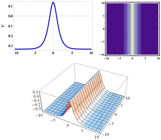
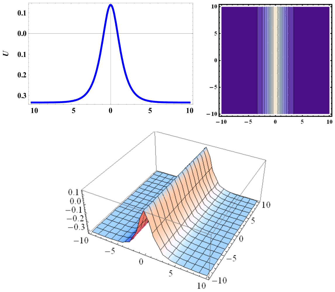
The solution corresponding to Equation (13) is illustrated in Figure 1.

Figure 1. For $k=2$, $l=3$, and $b=1$, the solution to Equation (13) is shown.

Equation (13) is physically significant due to the bright soliton structure. This is analyzed in Section 5 (An Artificial Neural Network Approach to the Gardner Equation).

$$U_4^{\pm }(\eta )=-{\displaystyle \frac{k+\sqrt{-2k^{2}mn}{\mathrm{csch}}_{mn}\left(\sqrt{b}\eta \right)}{2l}}.$$

(14)

Case 3: If $b<0$ and $a={\displaystyle \frac{b^2}{4}}$

$$U_5^{\pm }(\eta )=-{\displaystyle \frac{k+\sqrt{k^2}{\tanh }_{mn}\left(\sqrt{-\frac{b}{2}}\eta \right)}{2l}}$$

(15)

$$U_6^{\pm }(\eta )=-{\displaystyle \frac{k+\sqrt{k^2}{\coth }_{mn}\left(\sqrt{-\frac{b}{2}}\eta \right)}{2l}}$$

(16)

$$U_7^{\pm }(\eta )=-{\displaystyle \frac{k+\sqrt{k^2}\left({\tan h}_{mn}\left(\sqrt{-2b}\eta \right)+i\sqrt{mn}\sec h_{mn}\left(\sqrt{-2b}\eta \right)\right)}{2l}}$$

(17)

$$U_8^{\pm }(\eta )=-{\displaystyle \frac{k+\sqrt{k^2}\left(\cot h_{mn}\left(\sqrt{-2b}\eta \right)+\sqrt{mn}{\csc h}_{mn}\left(\sqrt{-2b}\eta \right)\right)}{2l}}$$

(18)

and

$$U_9^{\pm }(\eta )=-{\displaystyle \frac{k+\sqrt{\frac{k^2}{4}}\left({\tanh }_{mn}\left(\sqrt{\frac{-b}{8}}\eta \right)\right)+\sqrt{mn}{\coth }_{mn}\left(\sqrt{\frac{-b}{8}}\eta \right)}{2l}}$$

(19)

Case 4: If $b>0$ and $a={\displaystyle \frac{b^2}{4}}$

$$U_{10}^{\pm }(\eta )=-{\displaystyle \frac{k+\sqrt{-k^2}{\tan }_{mn}\left(\sqrt{\frac{b}{2}}\eta \right)}{2l}}$$

(20)

$$U_{11}^{\pm }(\eta )=-{\displaystyle \frac{k+\sqrt{-k^2}{\cot }_{mn}\left(\sqrt{\frac{b}{2}}\eta \right)}{2l}}$$

(21)

$$U_{12}^{\pm }(\eta )=-{\displaystyle \frac{k+\sqrt{-k^2}\left({\tan }_{mn}\sqrt{2b}\eta +\sqrt{mn}{\sec }_{mn}\sqrt{2b}\eta \right)}{2l}}$$

(22)

$$U_{13}^{\pm }(\eta )=-{\displaystyle \frac{k+\sqrt{-k^2}\left({\cot }_{mn}\sqrt{2b}\eta +\sqrt{mn}{\csc }_{mn}\sqrt{2b}\eta \right)}{2l}}$$

(23)

and

$$U_{14}^{\pm }(\eta )=-{\displaystyle \frac{k+\frac{\sqrt{-k^2}}{2}\left({\tan }_{mn}\left(\sqrt{\frac{b}{8}}\eta \right)-\sqrt{mn}{\cot }_{mn}\left(\sqrt{\frac{b}{8}}\eta \right)\right)}{2l}}$$

(24)

The above (11)–(24) analytical solutions are valid only under the (10) parameter constraints.

4. Artificial Neural Network Architecture Applied to the Gardner Equation

In this section, the ANN structure applied to the Gardner equation is presented.

4.1. Levenberg–Marquardt Algorithm

The Levenberg–Marquardt algorithm is an optimization method combining the advantages of the Gauss–Newton method with gradient descent, and it is commonly used in the training of ANNs because it provides stable and fast convergence, particularly in regions where the gradient of the error surface is low. The weight update formula is expressed as follows:

$$\Delta w=-{\left(J^{T}J+\mu I\right)}^{-1}{J}^{T}e\hspace{0.33em}.$$

Here, $\Delta w$ is the weight change, and $J$ is the Jacobian matrix of the residual error vector with respect to the network weights and biases. $e$ is the difference vector between the network’s outputs and the true values, $I$ is the identity matrix, and $\mu$ is the damping parameter that determines the algorithm’s behavior.

Throughout the training process, $\mu$ is adjusted adaptively. If the error decreases, $\mu$ decreases (approaching the Newton method), and if the error increases, $\mu$ increases (approaching gradient descent). Therefore, the Levenberg–Marquardt algorithm is a method that combines the speed of the Newton method with the stability of gradient descent, making it favorable for small and medium-sized datasets [26,32,33].

4.2. Training Process and Hyperparameters

To train ANNs successfully, simply selecting the right algorithms is not sufficient. The proper preparation of the dataset, the processing of input and output data, the separation of training and test data, and the correct selection of hyperparameters directly affect the performance. This section discusses the steps employed in training an ANN and the hyperparameters that affect model performance.

4.3. Activation Functions

Activation functions are mathematical operations that determine how each neuron generates an output based on its total input (weighted inputs and bias), enabling an ANN to model nonlinear relationships. Therefore, they have a direct impact on the network’s learning and generalization capabilities [23].

Activation functions are divided into two main categories: linear and nonlinear. The following functions are commonly used.

Sigmoid function

This function has been widely used in conventional neural network architectures. The output value ranges from 0 to 1, according to the following expression:

$$f\left(x\right)={\displaystyle \frac{1}{1+e^{-x}}}$$

This function has a limited output range and is sensitive to small changes, potentially leading to vanishing gradients [23].

Hyperbolic tangent function

The output value ranges from −1 to 1, and as the function produces symmetric outputs based on the sigmoid function, it is more advantageous and defined as follows [33]:

$$f\left(x\right)=\tanh \left(x\right)={\displaystyle \frac{e^x-e^{-x}}{e^x+e^{-x}}}$$

Linear activation function

This function is typically used in the output layer, as it passes the input directly to the output, which is preferred in regression problems. The form is expressed as follows [26]:

$$f\left(x\right)=x$$

4.4. Dataset Preparation and Normalization

Proper data preprocessing is critical for ensuring that the ANN model can learn accurately and quickly. This process typically consists of two main steps: dataset creation and scaling (normalization).

The dataset is defined as ${\left\{\left(x^{\left(i\right)},{\widehat{x}}^{\left(i\right)}\right)\right\}}_{i=1}^n$, where $x^{\left(i\right)}ϵR^d$ is the $d$-dimensional input vector for the sample $i.$, ${\widehat{x}}^{\left(i\right)}ϵR$ is the target output associated with the $i$-th sample, and $n$ denotes the total number of data samples.

The dataset is divided into training, validation, and test subsets using an appropriate partitioning strategy.

The scaling of input data in neural network training is particularly significant given the operating ranges of activation functions (e.g., [0, 1] for the sigmoid function or [−1, 1] for the tanh function). Wide or uneven data ranges can make learning difficult and prolong the model’s training time [23]. One of the most commonly used normalization methods is min–max scaling:

$$x^{norm}={\displaystyle \frac{x-x_{\min }}{x_{\max }-x_{\min }}}$$

where $x$ is the original input data, and $x_{\min }$ and $x_{\max }$ are the minimum and maximum values in the dataset.

Herein, the data are mapped to the range of [−1, 1] using this method. This process is automated in MATLAB R2019b, employing the mapminmax function [26].

4.5. Training, Validation, and Test Sets

The dataset is typically divided into three subsets to effectively train ANNs and evaluate their generalization ability: training set, validation set, and test set.

The primary purpose of this splitting is to ensure that the model does not merely memorize the training data but also achieves high accuracy on data it has not seen. Each subset is listed below:

• Training set: used to update weights.
• Validation set: measured the model’s generalization ability during the training process and can be used as an early stopping criterion.
• Test set: used to measure the model’s final performance after training is complete.

The following ratios are most commonly used for dividing the dataset into these subsets:

• Training: 70%; validation: 15%; and test: 15%.
• Training: 80%; validation: 10%; and test: 10%.

These ratios can be adjusted depending on the application; for example, alternative methods (e.g., cross-validation) may be preferred in studies with limited data. Data splitting is typically performed in MATLAB R2019b using the dividerand function, which randomly divides the entire dataset based on the specified ratios:

$$\left[x_{train},x_{val},x_{test}\right]=\mathrm{dividerand}\left(x,0.7,0.15,0.15\right)$$

Similarly, the target outputs are divided by the same ratios. During this process, the input–output mappings should be preserved [26].

4.6. Hyperparameters

Properly selecting the hyperparameters is just as important as selecting the training algorithm in terms of ANN performance. Hyperparameters are determined before the training process begins, and they directly influence the model’s learning behavior. This section discusses hyperparameters commonly used in ANN training, and the rationale for their selection is supported by mathematical expressions.

4.7. Epoch Number

An epoch refers to one cycle of the network processing all the training data. The training process typically consists of multiple epochs. The appropriate number of epochs determines how long the model continues to learn. If the number of epochs is too low, the network cannot learn sufficiently, but if it is set too high, the risk of overfitting increases [33]. The network typically updates the weights during the epoch:

$$w_{ij}^{\left(t+1\right)}=w_{ij}^{\left(t\right)}-\eta .{\displaystyle \frac{\partial E}{\partial w_{ij}}}$$

(25)

where $w_{ij}$ is the weight from neuron $i$ to neuron $j$, $w_{ij}^{(t+1)}$ is the updated weight value in the next iteration, $\eta$ is the learning coefficient, $E$ is the error (loss) function, and ${\displaystyle \frac{\partial E}{\partial w_{ij}}}$ is the gradient of the error function with respect to the relevant weight.

4.8. Learning Coefficient

The learning rate determines the magnitude of the weight updates made in each iteration. If it is set too low, the learning process slows down, but if it is set too high, the learning process may become unstable [23]. The weight function is formulated in Equation (25).

4.9. Number of Hidden Layers and Neurons

Another critical parameter defining the structure of a neural network is the number of hidden layers and the number of neurons in each layer. Single-hidden-layer feedforward networks can, in theory, approximate any continuous function. However, multiple hidden layers and a larger number of neurons may be required for highly complex problems [26]. This structure is expressed as follows:

$$h_j=f\left({\displaystyle \sum _{i=1}^n{w}_{ji}.x_i+b_j}\right)$$

where $h_j$ is the output of neuron $j$ in the hidden layer, $f\left(.\right)$ is the activation function, $x_i$ is the input data, $w_{ji}$ is the weight, and $b$ is the bias.

4.10. Mean Squared Error

The mean squared error (MSE) is a performance metric representing the average of the squares of the differences between the values predicted by the model and the actual values. The formula is as follows:

$$\mathrm{MSE}={\displaystyle \frac{1}{n}}{{\displaystyle \sum _{i=1}^n\left(x_i-{\widehat{x}}_i\right)}}^2$$

where $x_i$ indicates real values, ${\widehat{x}}_i$ denotes the values predicted by the model, and $n$ is the number of data. MSE is a widely used error function, particularly for regression problems. As the MSE value approaches zero, the model’s predictive performance improves [28,34].

5. An Artificial Neural Network Approach to the Gardner Equation

The data obtained from certain analytical solutions of the Gardner equation were evaluated to generate approximate solutions using a feedforward neural network model. This model comprises a classical architecture in which data are transmitted only in the forward direction (from the input layer to the output layer) and does not include a feedback structure. The training process was carried out based on the backpropagation algorithm.

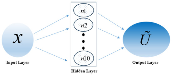
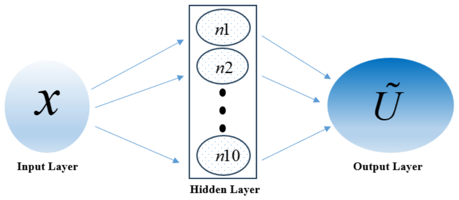
The feedforward artificial neural network employed in this study consisted of a single hidden layer containing 10 neurons. A single-hidden-layer architecture was selected because, according to the universal approximation theorem, such networks are capable of approximating continuous nonlinear functions with arbitrary accuracy when an adequate number of neurons are employed while maintaining relatively low computational complexity [35]. A very low number of neurons can limit the model’s learning power, whereas a very high number of neurons can increase training time and negatively impact generalization performance. Since each dataset contained input–output samples corresponding to uniformly spaced spatial points, a network architecture was considered appropriate to reduce the possibility of overfitting and to ensure stable training [23,36]. Therefore, 10 hidden neurons were adopted as a practical compromise between approximation accuracy, computational efficiency, and model simplicity for the present problem.

The nonlinear hyperbolic tangent activation function was chosen for the hidden layer, whereas the linear activation function was selected for the output layer. The hyperbolic tangent function transforms input values to a range between −1 and 1, allowing neurons to produce linear outputs, and the linear activation function enables the generation of output values across a wide range, making it preferable in regression-type problems [26,33].

In the ANN implementation, only the spatial variable x was used as the network input. The time variable t was treated as a fixed parameter and was not included as an input feature. For each selected time level, the corresponding analytical solution values were generated separately and used as the target dataset, while the same ANN architecture and training procedure were maintained throughout the study. The network’s input data consist of position values at specific time steps; the target outputs contain the corresponding $\tilde{U}$ solution values, and the network generates approximate solutions by learning these input–output mappings.

The number of epochs was set to 1000 during model training, with data split into training (70%), validation (15%), and test (15%) sets. The input and output data were normalized using the mapminmax function in MATLAB R2019b before being fed into the ANN. This process scales the data within the range [−1, 1] based on the minimum and maximum values in each dataset. All input values are expressed within the same range; therefore, the network can evaluate each input at a similar level, preventing data with large numerical values from dominating over smaller ones during training. This ensures that the learning process is both fast and stable.

The Levenberg–Marquardt algorithm was selected in the training process. It is an improved version of the classical gradient descent method and performs with high success on small and medium-sized datasets by utilizing the Gauss–Newton technique. Owing to its fast convergence property, it is highly effective in regression problems based on differential equations [27,37,38,39,40]. Additionally, this algorithm does not require a fixed learning rate but operates through a damping coefficient ($\mu$) that automatically adjusts the step size, eliminating the need for the user to manually define a learning rate; the algorithm adapts itself and continues the optimization with appropriate step sizes. This also facilitates quick and stable learning for the model.

MSE was adopted as the performance metric because the present study addresses a function approximation (regression) problem. MSE quantifies the average squared difference between the ANN predictions and the corresponding analytical solution values while assigning greater weight to larger prediction errors. This property makes MSE particularly suitable for training and evaluating neural networks in regression tasks and is therefore widely employed in the literature [28]. Low error rates indicate that the model can generate approximate solutions with high accuracy. Figure 2 illustrates the general structure of the model. The input layer includes the data, which are processed by the 10 neurons in the hidden layer, and the $\tilde{U}$ estimation is obtained in the output layer.

Figure 2. Illustration of the feedforward ANN model used in this study.

The ANN model was trained several times due to the random initialization of network weights and random data partitioning. The model providing the best regression performance and the lowest prediction error was selected for the analyses presented in this study. A statistical analysis based on different normalization ranges or fixed random seeds was beyond the scope of the present work. Network training was terminated in the MATLAB R2019b program when the specified minimum gradient threshold was reached, which ensures that the network has achieved the desired performance level and does not require further training.

In this study, the ANN was trained using the analytical solution corresponding to Equation (13). The approximate solution graphs, regression graphs, and tables comparing the analytical and ANN solutions for $t=0$ and $t=8$ (i.e., the time steps determined for the Gardner equation) are provided below.

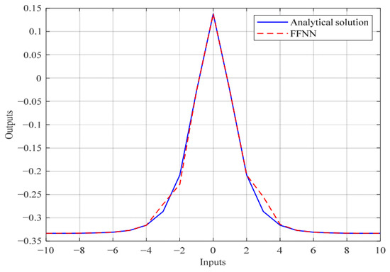
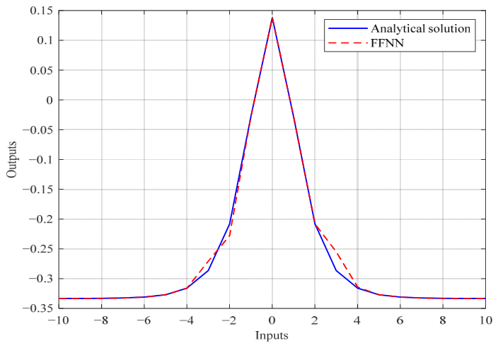
Figure 3 compares the analytical solution of the Gardner equation (Equation (13)) with the approximation obtained by the proposed ANN model. It is observed that the ANN prediction closely follows the analytical solution over the entire spatial domain, with only minor deviations near the region where the solution gradient is the highest. The approximate solution curve obtained from the ANN model overlaps significantly with the analytical solution curve, particularly outside the $2<x<4$ range. This agreement shows that the model successfully learned the solution structure at the initial time step.

Figure 3. Comparison of the analytical and ANN outputs at $t=0$ for the solution to the Gardner equation (Equation (13)).

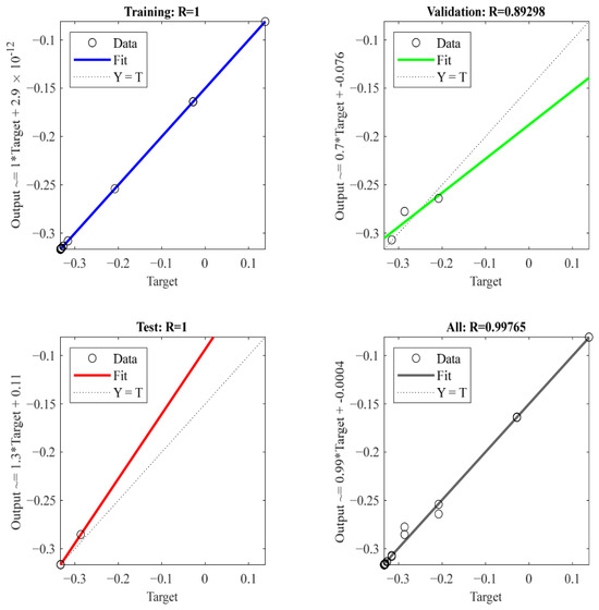
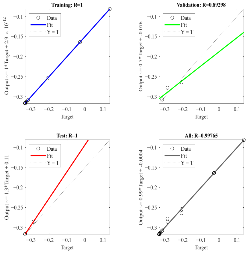
Figure 4 shows the regression relationships between the target values and the ANN outputs at time $t=0$ for the training, validation, test, and total sets. The correlation coefficients (R) are shown separately for each graph. Perfect agreement (R = 1) was obtained for both the training and test data. While the validation subset yielded a slightly lower value (R = 0.89298), the correlation for the dataset remained high (R = 0.99765).

Figure 4. Regression graphs showing the relationships between the target and output values at $t=0$ for the solution to the Gardner equation (Equation (13)).

Table 1 provides a point-by-point comparison between the analytical and ANN solutions calculated for specific $x$ and $y$ values at $t=0$. The $x$ and $y$ test points were selected to be symmetrical and equally spaced, ensuring a balanced assessment of model performance across the defined range. The last column lists the absolute error between the analytical solution and the ANN solutions at each test point.

Table 1. Comparison of the analytical and ANN outputs at $t=0$ for the solution to Equation (13).

$\mathit{x}$	$\mathit{y}$	Analytical Solution	ANN	Error
−10	−10	−0.333290529869154	−0.333290529644426	$2.2473\times {10}^{-10}$
−8	−8	−0.3330170561702263	−0.333013750955364	$3.3052\times {10}^{-6}$
−6	−6	−0.3309963577282055	−0.330996361673878	$3.9457\times {10}^{-9}$
−4	−4	−0.3160709742630202	−0.316070975333110	$1.0701\times {10}^{-9}$
−2	−2	−0.208032961024616	−0.228052040076727	0.0200
0	0	0.138071187457698	0.138071187444684	$1.3014\times {10}^{-11}$
2	2	−0.208032961024616	−0.208032961966403	$9.4179\times {10}^{-10}$
4	4	−0.3160709742630202	−0.314110212551543	0.0020
6	6	−0.3309963577282055	−0.330996365275372	$7.5472\times {10}^{-9}$
8	8	−0.3330170561702263	−0.332979893689757	$3.7162\times {10}^{-5}$
10	10	−0.333290529869154	−0.333290529737714	$1.3144\times {10}^{-10}$

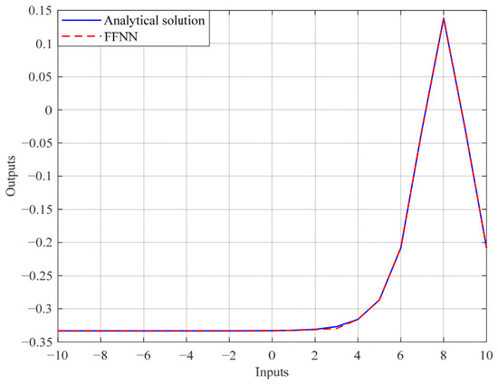
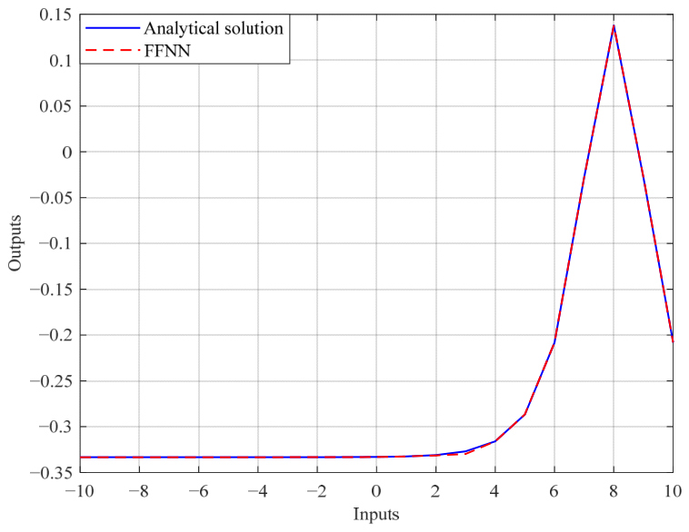
Figure 5 compares the analytical and ANN solutions at $t=8$ for the solution to Equation (13). The ANN output closely follows the analytical solution curve, indicating that the model can correctly learn and generalize the solution structure not only at the initial time steps but also at later time steps.

Figure 5. Comparison of the analytical and ANN outputs at time $t=8$ for the solution to the Gardner equation (Equation (13)).

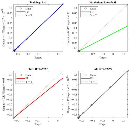
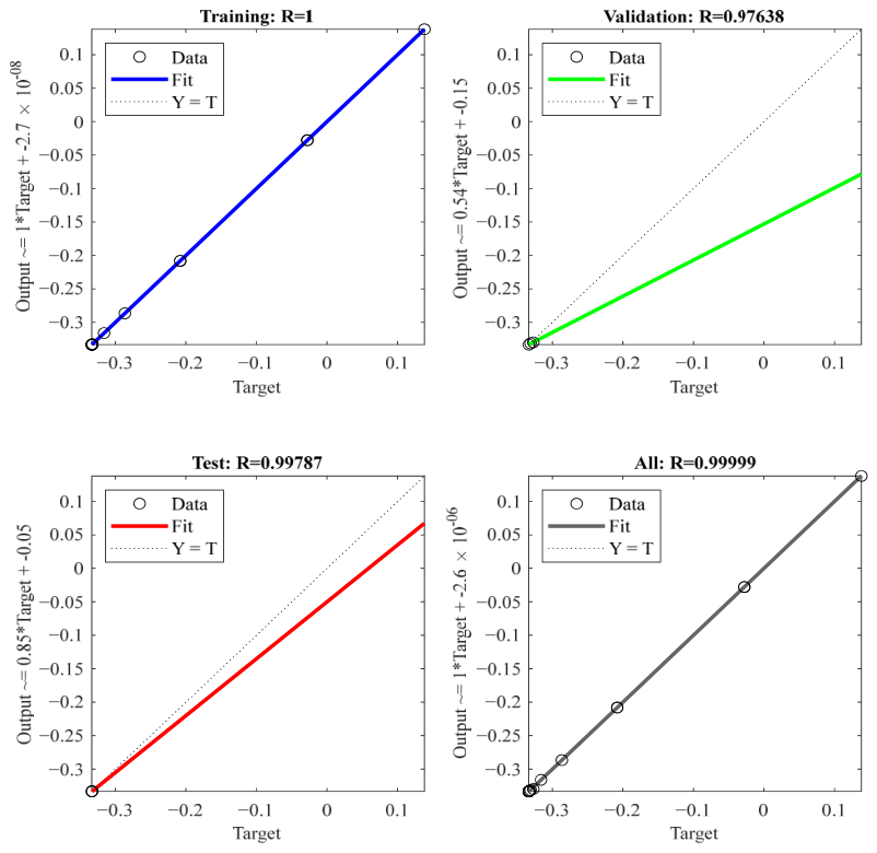
Figure 6 shows the corresponding regression plots for the training, validation, test, and total datasets at $t=8$. The correlation coefficient reaches R = 0.99999 for the total dataset, indicating high prediction accuracy. The high R values obtained for the training and test datasets indicate that the proposed ANN model provides accurate predictions and exhibits satisfactory generalization performance, as supported by an R value of 0.97638 in the validation set.

Figure 6. Regression graphs showing the relationships between the target and output values at $t=8$ for the solution to the Gardner equation (Equation (13)).

Table 2 presents a point-by-point comparison between the analytical solution and the ANN outputs at $t=8$. The predicted values remain in close agreement with the analytical solution across the computational domain. The reported differences between the analytical solution and the ANN outputs for specific $x$ and $y$ values, along with the corresponding error values, are shown. The absolute error values demonstrate that the ANN model consistently produces results proximal to the analytical solution, maintaining high accuracy at $t=8$ and obtaining the solution to the Gardner equation successfully.

Table 2. Comparison of the analytical and ANN outputs at $t=8$ for the solution to Equation (13).

$\mathit{x}$	$\mathit{y}$	Analytical Solution	ANN	Error
−10	−10	−0.333333318974371	−0.333333317303634	$1.6707\times {10}^{-9}$
−8	−8	−0.333333227234153	−0.333333658245799	$4.3101\times {10}^{-7}$
−6	−6	−0.333332549360539	−0.333335350494493	$2.8011\times {10}^{-6}$
−4	−4	−0.333327540514373	−0.333351447085781	$2.3907\times {10}^{-5}$
−2	−2	−0.333290529869154	−0.333292359625350	$1.8298\times {10}^{-6}$
0	0	−0.3330170561702263	−0.333076648030519	$5.9592\times {10}^{-5}$
2	2	−0.3309963577282055	−0.331378754248658	$3.8240\times {10}^{-4}$
4	4	−0.3160709742630202	−0.316070347000061	$6.2726\times {10}^{-7}$
6	6	−0.208032961024616	−0.208032972253681	$1.1229\times {10}^{-8}$
8	8	0.138071187457698	0.138071185451213	$2.0065\times {10}^{-9}$
10	10	−0.208032961024616	−0.208032961027235	$2.6190\times {10}^{-12}$

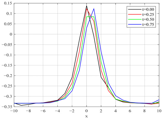
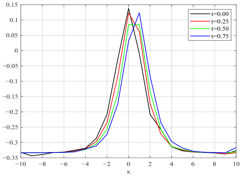
Figure 7 displays the approximate solutions obtained using the ANN model at various time steps ($t=0.00$, $0.25$, $0.50$, and $0.75$). For each time level, the ANN model was trained and evaluated using the corresponding analytical dataset generated from Equation (13). The curves in Figure 7 show that the model captures the temporal evolution of the solution structure, which does not change significantly with time. The continuity and similarity among the curves suggest that the ANN model can produce valid solutions not only for discrete time points but also over a continuous time interval. The ANN model’s ability to produce smooth transitions and maintain accuracy across different time steps underscores its capability to learn time-sensitive structural changes in nonlinear systems.

Figure 7. Comparative graph of the approximate solutions obtained using the ANN model at different time steps ($t=0.00,0.25,0.50,0.75$) for the solution to the Gardner equation (Equation (13)).

6. Results and Discussion

In this study, it is demonstrated that the feedforward artificial neural network (ANN) approximates the analytical solution of the Gardner equation over the considered spatial domain and at different time levels. The ANN learns the nonlinear coupling between the input variables and the corresponding analytic solution values using supervised training. After the learning stage, the trained network is capable of rapidly producing solution approximations for new input points within the considered domain. Such nonlinear function approximation capability is one of the major advantages of feedforward neural networks and has been extensively reported in the neural network literature [23,26,33].

Although the prediction errors remain small throughout the computational domain, slightly larger local errors are observed at a limited number of spatial points. These locations correspond to regions where the analytical solution exhibits relatively steeper gradients, making the approximation task more demanding for a neural network. Such localized deviations are expected in data-driven approximation models and do not affect the overall prediction quality, as confirmed by the high regression coefficients and the low absolute error values [26,36].

Another important observation is that the ANN maintains approximation accuracy at different time levels. Independent training and testing were carried out using the analytical datasets generated for each selected time instant, and the obtained results consistently demonstrate agreement with the corresponding analytical solutions. This demonstrates that the proposed ANN can accurately reproduce the solution profiles not only at the initial time but also at later time levels within the investigated time interval.

The objective of the present study was to investigate whether a feedforward ANN can accurately approximate the analytical solutions obtained for the Gardner equation using the Sardar sub-equation method. Therefore, the analytical solution was intentionally adopted as the reference solution for performance evaluation [32,37,38].

The primary contribution of this study lies in the successful application of the Sardar sub-equation method to generate analytical solutions and in demonstrating that these solutions can be accurately approximated using a feedforward artificial neural network. In this study, the ANN does not independently solve the Gardner equation; instead, it learns the mapping represented by the analytical reference data. Therefore, the present study does not include external validation using independently generated datasets or benchmark comparisons with alternative numerical approaches. In addition, the present results should be interpreted as demonstrating the approximation capability of the ANN. The obtained results indicate that the proposed ANN model provides an accurate and computationally efficient approximation for the Gardner equation within the investigated domain. The combination of analytical solutions for data generation and ANN-based approximation offers a practical strategy that may be extended to nonlinear partial differential equations with variable coefficients where repeated evaluations of the solution are required.

7. Conclusions

In this study, soliton wave solutions for the Gardner equation were first derived by applying the Sardar sub-equation method. The accuracy of these results was verified by substituting the resulting functions and their derivatives back into the governing equation. Systematic application of the Sardar sub-equation method yielded both hyperbolic and trigonometric analytical solutions. Notably, the bright soliton structure identified in Equation (13) and illustrated in Figure 1 is of significance, considering that bright solitons are fundamental to the distortion-free transmission of light pulses over long distances in optical fibers. The results confirm that the Sardar sub-equation method is a powerful and systematic method, and it is also a robust tool for generating soliton solutions to nonlinear PDEs.

Next, a feedforward ANN model was developed using the Levenberg–Marquardt algorithm to obtain solutions of the Gardner equation. In this model architecture, featuring a hidden layer of 10 neurons, error performance was evaluated based on the MSE. Following the training process, the model fit the sample data obtained from the analytical solution with high precision and minimal error. In the final section of the study, comparative graphical analysis of the numerical solutions generated by the ANN model at various time steps demonstrated that the curves and analytical solution structures obtained were nearly identical. As a result of the evaluations conducted on the test data after the training was completed, it was observed that the model could produce results with accuracy. Future studies addressing the derivation of solutions to nonlinear PDEs are expected to open new areas of research and application through the use of ANNs.

References

- Alam, N.; Akbar, M.A. Traveling wave solutions for the mKdV equation and the Gardner equations by new approach of the generalized (G′/G)-expansion method. J. Egypt. Math. Soc. 2014, 22, 402–406. [Google Scholar] [CrossRef] [Scilit]
- Betchewe, G.; Victor, K.K.; Thomas, B.B.; Crepin, K.T. New solutions of the Gardner equation: Analytical and numerical analysis of its dynamical understanding. Appl. Math. Comput. 2013, 223, 377–388. [Google Scholar] [CrossRef] [Scilit]
- Biswas, A.; Zerrad, E. Soliton perturbation theory for the Gardner equation. Adv. Stud. Theor. Phys. 2008, 2, 787–794. [Google Scholar]
- Dağhan, D.; Dönmez, O. Exact solutions of the Gardner equation and their applications to the different physical plasmas. Braz. J. Phys. 2016, 46, 321–333. [Google Scholar] [CrossRef] [Scilit]
- Kamchatnov, A.M.; Kuo, Y.-H.; Lin, T.-C.; Horng, T.-L.; Gou, S.-C.; Clift, R.; El, G.A.; Grimshaw, R.H.J. Undular bore theory for the Gardner equation. Phys. Rev. E—Stat. Nonlinear Soft Matter Phys. 2012, 86, 036605. [Google Scholar] [CrossRef] [Scilit] [PubMed]
- Vassilev, V.M.; Djondjorov, P.A.; Hadzhilazova, M.T.; Miadenov, I.M. Traveling wave solutions of the Gardner equation and motion of plane curves governed by the mKdV flow. AIP Conf. Proc. 2011, 1404, 86–93. [Google Scholar] [CrossRef] [Scilit]
- Yıldız, G.; Turkmen, Ç. Application of Kudryashov method to some equations used in physics science. J. Sci. Technol. 2019, 12, 1485–1492. [Google Scholar] [CrossRef] [Scilit]
- Fu, Z.; Liu, S.; Liu, S. New kinds of solutions to Gardner equation. Chaos Solitons Fractals 2004, 20, 301–309. [Google Scholar] [CrossRef] [Scilit]
- Wazwaz, A.-M. New solitons and kink solutions for the Gardner equation. Commun. Nonlinear Sci. Numer. Simul. 2007, 12, 1395–1404. [Google Scholar] [CrossRef] [Scilit]
- Raut, S.; Ma, W.-X.; Barman, R.; Roy, S. A non-autonomous Gardner equation and its integrability: Solitons, positons and breathers. Chaos Solitons Fractals 2023, 176, 114089. [Google Scholar] [CrossRef] [Scilit]
- Verheest, F.; Hereman, W.A. The Gardner equation and acoustic solitary waves in plasmas. J. Plasma Phys. 2025, 91, E117. [Google Scholar] [CrossRef] [Scilit]
- Debin, K.; Rezazadeh, H.; Ullah, N.; Vahidi, J.; Tariq, K.U.; Akinyemi, L. New soliton wave solutions of a (2 + 1)-dimensional Sawada-Kotera equation. J. Ocean Eng. Sci. 2022, 8, 527–532. [Google Scholar] [CrossRef] [Scilit]
- Esen, H.; Ozdemir, N.; Secer, A.; Bayram, M. On solitary wave solutions for the perturbed Chen–Lee–Liu equation via an analytical approach. Optik 2021, 245, 167641. [Google Scholar] [CrossRef] [Scilit]
- Hussain, R.; Imtiaz, A.; Rasool, T.; Rezazadeh, H.; Inc, M. Novel exact and solitary solutions of conformable Klein–Gordon equation via Sardar-subequation method. J. Ocean Eng. Sci. 2022. [Google Scholar] [CrossRef] [Scilit]
- Rahman, H.U.; Asjad, M.I.; Munawar, N.; Parvaneh, F.; Muhammad, T.; Hamoud, A.A.; Emadifar, H.; Hamasalh, F.K.; Azizi, H.; Khademi, M. Traveling wave solutions to the Boussinesq equation via Sardar sub-equation technique. AIMS Math. 2022, 7, 11134–11149. [Google Scholar] [CrossRef] [Scilit]
- Rehman, H.U.; Asjad, M.I.; Inc, M.; Iqbal, I. Exact solutions for new coupled Konno–Oono equation via Sardar subequation method. Opt. Quant. Electron. 2022, 54, 798. [Google Scholar] [CrossRef] [Scilit]
- Rehman, H.U.; Iqbal, I.; Aiadi, S.S.; Mlaiki, N.; Saleem, M.S. Soliton Solutions of Klein–Fock–Gordon equation using Sardar subequation method. Mathematics 2022, 10, 3377. [Google Scholar] [CrossRef] [Scilit]
- Rehman, H.U.; Akber, R.; Wazwaz, A.-M.; Alshehri, H.M.; Osman, M.S. Analysis of Brownian motion İn stochastic schrödinger wave equation using Sardar sub-equation method. Optik 2023, 289, 171305. [Google Scholar] [CrossRef] [Scilit]
- Rezazadeh, H.; Inc, M.; Baleanu, D. New solitary wave solutions for variants of (3+1)-dimensional Wazwaz-Benjamin-Bona-Mahony equations. Front. Phys. 2020, 8, 332. [Google Scholar] [CrossRef] [Scilit]
- Pleumpreedaporn, C.; Moore, E.J.; Sirisubtawee, S.; Khansai, N.; Pleumpreedaporn, S. Exact solutions for the Sharma–Tasso–Olver equation via the Sardar subequation method with a comparison between Atangana space–time beta-derivatives and classical derivatives. Mathematics 2024, 12, 2155. [Google Scholar] [CrossRef] [Scilit]
- Tariq, H.; Ashraf, H.; Rezazadeh, H.; Demirbilek, U. Travelling wave solutions of nonlinear conformable Bogoyavlenskii equations via two powerful analytical approaches. Appl. Math. J. Chin. Univ. 2024, 39, 502–518. [Google Scholar] [CrossRef] [Scilit]
- Yasin, S.; Khan, A.; Ahmad, S.; Osman, M.S. New exact solutions of (3+1)-dimensional modified KdV-Zakharov-Kuznetsov equation by Sardar-subequation method. Opt. Quantum Electron. 2024, 56, 90. [Google Scholar] [CrossRef] [Scilit]
- Goodfellow, I.; Bengio, Y.; Courville, A. Deep Learning; MIT Press: Cambridge, MA, USA, 2016. [Google Scholar]
- LeCun, Y.; Bengio, Y.; Hinton, G. Deep learning. Nature 2015, 521, 436–444. [Google Scholar] [CrossRef] [Scilit] [PubMed]
- Li, Z.; Wu, M.; Hussain, E.; Yildirim, Y. Exactly explicit solutions of (2+1)-dimensional conformable fractional diffusive Predator–Prey model via neural networks method. Front. Phys. 2026, 14, 1824530. [Google Scholar] [CrossRef] [Scilit]
- Hagan, M.T.; Demuth, H.B.; Beale, M.H.; De Jesus, O. Neural Network Design, 2nd ed.; Martin Hagan Publishing: Stillwater, OK, USA, 2014. [Google Scholar]
- Wilamowski, B.M.; Yu, H. Improved computation for Levenberg-Marquardt training. IEEE Trans. Neural Netw. 2010, 21, 930–937. [Google Scholar] [CrossRef] [Scilit] [PubMed]
- Chicco, D.; Warrens, M.J.; Jurman, G. The coefficient of determination R-squared is more informative than SMAPE, MAE, MAPE, MSE and RMSE in regression analysis evaluation. PeerJ Comput. Sci. 2021, 7, e623. [Google Scholar] [CrossRef] [Scilit] [PubMed]
- Chiu, C.-T.; Mehrotra, K.; Mohan, C.K.; Ranka, S. Robustness of feedforward neural networks. IEEE Int. Conf. Neural Netw. 1993, 2, 783–788. [Google Scholar] [CrossRef] [Scilit]
- Teso-Fz-Betoño, A.; Zulueta, E.; Cabezas-Olivenza, M.; Teso-Fz-Betoño, D.; Fernandez-Gamiz, U. A study of learning issues in feedforward neural networks. Mathematics 2022, 10, 3206. [Google Scholar] [CrossRef] [Scilit]
- Cuomo, S.; Di Cola, V.S.; Giampaolo, F.; Rozza, G.; Raissi, M.; Piccialli, F. Scientific machine learning through physics-informed neural networks: Where we are and what’s next. J. Sci. Comput. 2022, 92, 88. [Google Scholar] [CrossRef] [Scilit]
- Huang, G.-B.; Zhu, Q.-Y.; Siew, C.-K. Extreme learning machine: Theory and applications. Neurocomputing 2006, 70, 489–501. [Google Scholar] [CrossRef] [Scilit]
- Haykin, S. Neural Networks and Learning Machines, 3rd ed.; Pearson Education: London, UK, 2009. [Google Scholar]
- Noor, A.Z.; Fauadi, M.H.F.M.; Jafar, F.A.; Bakar, M.H.A. Optimal number of hidden neuron identification for sustainable manufacturing application. Int. J. Recent Technol. Eng. 2019, 8, 2447–2453. [Google Scholar] [CrossRef] [Scilit]
- Petersen, P.; Voigtlaender, F. Optimal approximation of piecewise smooth functions using deep ReLU neural networks. Neural Netw. 2018, 108, 296–330. [Google Scholar] [CrossRef] [Scilit] [PubMed]
- Geron, A. Hands on Machine Learning with Scikit-Learn, Keras and TensorFlow, 3rd ed.; O’Reilly Media: Sebastopol, CA, USA, 2022. [Google Scholar]
- Sun, H.; Hou, M.; Yang, Y.; Zhang, T.; Weng, F.; Han, F. Solving partial differential equation based on Bernstein neural network and extreme learning machine algorithm. Neural Process. Lett. 2019, 50, 1153–1172. [Google Scholar] [CrossRef] [Scilit]
- Chen, Y.; Yu, H.; Meng, X.; Xie, X.; Hou, M.; Chevallier, J. Numerical solving of the generalized Black-Scholes differential equation using Laguerre neural network. Digit. Signal Process. 2021, 112, 103003. [Google Scholar] [CrossRef] [Scilit]
- Pal, S.K.; Chakraborty, D. Surface roughness prediction in turning using artificial neural network. Neural Comput. Appl. 2005, 14, 319–324. [Google Scholar] [CrossRef] [Scilit]
- Malek, A.; Beidokhti, R.S. Numerical solution for high order differential equations using a hybrid neural network—Optimization method. Appl. Math. Comput. 2006, 183, 260–271. [Google Scholar] [CrossRef] [Scilit]
Disclaimer/Publisher’s Note: The statements, opinions and data contained in all publications are solely those of the individual author(s) and contributor(s) and not of MDPI and/or the editor(s). MDPI and/or the editor(s) disclaim responsibility for any injury to people or property resulting from any ideas, methods, instructions or products referred to in the content. |
© 2026 by the authors. Licensee MDPI, Basel, Switzerland. This article is an open access article distributed under the terms and conditions of the Creative Commons Attribution (CC BY) license.