A Dual-Factor-Driven Temporal Network for Pixel-Level NDVI Prediction in the Hulunbuir Grassland

Abstract

Normalized Difference Vegetation Index (NDVI) is an important remote sensing indicator for characterizing vegetation growth status and ecosystem changes. Improving NDVI prediction accuracy is of great significance for regional ecological monitoring and conservation. However, existing prediction methods often rely on single meteorological drivers or numerous explanatory variables that are difficult to obtain for future periods, limiting their applicability to pixel-level NDVI forecasting over spatially distributed areas. In this study, a Dual-Factor-Driven Temporal Network (DfT-Net) was proposed for pixel-level NDVI prediction in the Hulunbuir grassland based on MODIS NDVI data and ERA5-Land temperature and precipitation data from 2013 to 2024. The model was independently applied to valid 1000 m grassland pixels, with the same model parameters shared across pixels. This pixel-wise prediction strategy enables the model to learn common meteorological–vegetation response patterns across different pixels while generating spatially distributed NDVI predictions. For temporal feature modeling, Time Series Decomposition (TSD) was first applied to the temperature and precipitation sequences to decompose them into trend, seasonal, and residual components, thereby characterizing their multi-scale temporal variations and recurrent seasonal patterns. Subsequently, one-dimensional convolutional neural networks (CNNs) and long short-term memory networks (LSTMs) were employed to extract local temporal patterns and long-term temporal dependencies, respectively. Experimental results showed that DfT-Net achieved an RMSE of 0.100, an MAE of 0.074, and an R² of 0.828 on the independent temporal test set (2022–2024). Under the same experimental setting, DfT-Net achieved the lowest RMSE and MAE and the highest R² among the evaluated models, including LSTM, CNN, TSD-CNN, TSD-LSTM, and CNN-LSTM. These results indicate that DfT-Net effectively integrates dual-factor meteorological driving, multi-scale temporal feature representation, and pixel-level prediction, providing a useful framework for spatially distributed grassland NDVI forecasting and ecological monitoring.

1. Introduction

Vegetation is a fundamental component of terrestrial ecosystems, serving as a critical link among soil, hydrological, and atmospheric processes and acting as an important indicator of global environmental change. The quality and ecosystem services provided by vegetation constitute an essential foundation for sustainable human development [1]. Among various remote sensing indicators, the Normalized Difference Vegetation Index (NDVI) is one of the most widely used parameters for characterizing vegetation growth status and monitoring ecosystem dynamics. It provides reliable information on vegetation health and spatial distribution and has therefore become a key indicator in terrestrial ecosystem studies [2,3]. Continuous monitoring and accurate prediction of NDVI are essential for tracking ecosystem dynamics, understanding vegetation evolution mechanisms, and assessing ecosystem health. With the rapid development of smart agriculture and precision livestock management, reliable monthly NDVI forecasting has become increasingly important for crop management, grazing planning, agricultural yield estimation, and sustainable grassland utilization. Vegetation growth generally exhibits pronounced seasonal periodicity and recurrent interannual evolution, whereby similar growth stages tend to follow comparable temporal patterns. This temporal (seasonal) symmetry embedded in vegetation time series provides valuable prior information for vegetation forecasting. Effectively exploiting such temporal symmetric structures while incorporating meteorological drivers has therefore become an important research direction for improving NDVI prediction.

Studies on vegetation driving mechanisms have demonstrated that understanding the relationships between NDVI and meteorological variables is fundamental to predictive modeling. Previous studies have shown that the effects of temperature and precipitation vary considerably among different vegetation types [4]. In the Loess Plateau, vegetation cover has been reported to be highly sensitive to fluctuations in both temperature and precipitation [5]. In contrast, studies conducted in Hulunbuir, Inner Mongolia, indicate that temperature is the dominant factor controlling forest growth in the Greater Khingan Mountains, whereas precipitation plays a decisive role in maintaining grassland ecological stability and supporting regional agricultural and pastoral production [6,7]. These findings suggest that the synergistic effects of temperature and precipitation jointly determine the spatiotemporal dynamics of grassland NDVI.

With advances in mathematical modeling and computer science, NDVI prediction methods have evolved from conventional statistical approaches to deep learning techniques. Early studies mainly employed methods such as gray prediction models and support vector machines (SVMs) for vegetation dynamics simulation [8,9,10]. More recently, deep learning architectures represented by convolutional neural networks (CNNs) and recurrent neural networks (RNNs) have demonstrated remarkable advantages in NDVI prediction owing to their powerful nonlinear feature extraction capabilities [11]. For example, Pan et al. [12] employed ConvLSTM to capture the spatiotemporal dependencies of NDVI, while Reddy et al. [13] and Zhao et al. [14] achieved promising short- and medium-term prediction performance using LSTM-based models and their variants.

Despite these advances, several challenges remain in existing NDVI prediction studies. First, existing studies differ considerably in their choice of external driving factors. Some models rely primarily on historical NDVI sequences, which simplifies data requirements but may not adequately capture the effects of changing climatic conditions on vegetation dynamics. Other approaches incorporate multiple auxiliary variables, such as soil moisture, radiation, vegetation characteristics, and other remote-sensing or environmental factors [15,16,17]. These multi-factor models can provide richer explanatory information and improve predictive performance; however, some predictors may not be directly available for future prediction periods and may require additional forecasting models or future remote-sensing observations. This increases data acquisition and preprocessing requirements and limits their direct applicability to future NDVI forecasting based on readily available meteorological predictions. Therefore, a more parsimonious framework that uses key meteorological drivers as external inputs is desirable for practical future forecasting. Second, existing models do not always adequately characterize the multi-scale temporal structure of meteorological drivers. Although seasonal variables or meteorological factors have been incorporated into some NDVI prediction models [16], temperature and precipitation time series generally contain distinct trend, seasonal, and irregular fluctuation components. Directly treating these mixed signals as undifferentiated sequences may make it difficult for deep learning models to distinguish periodic patterns from irregular disturbances. Time-series decomposition provides an effective strategy for separating these components and has been shown to facilitate the extraction of characteristic temporal patterns and improve prediction performance [17,18]. However, the integration of meteorological time-series decomposition with dual-factor-driven NDVI forecasting, particularly for pixel-level prediction across spatially distributed grassland areas, remains insufficiently explored. Third, existing studies adopt different strategies for the spatial scale of NDVI prediction. Point-based or regional-mean forecasting methods can effectively characterize temporal evolution at specific locations or aggregated spatial scales, but they may not directly provide pixel-level predictions that preserve the spatial distribution and heterogeneity of vegetation dynamics across large grassland regions. Although spatial or spatiotemporal deep learning approaches can explicitly model spatial relationships, they often require spatial image sequences, neighboring-pixel information, or a relatively large number of explanatory variables [19,20,21,22]. Such requirements may increase model complexity and data-processing costs and may be difficult to satisfy when the objective is future NDVI forecasting using a limited set of meteorological predictors. Therefore, there remains a need for a relatively simple temporal forecasting framework that can use practically obtainable meteorological drivers to predict NDVI independently at spatially distributed pixels while preserving the spatial distribution of the resulting predictions.

To address these limitations, this study proposes a Dual-Factor-Driven Temporal Network (DfT-Net) for monthly pixel-level NDVI prediction using MODIS NDVI data together with ERA5-Land temperature and precipitation data collected over the Hulunbuir grassland during 2013–2024. The model is independently applied to valid 1000 m grassland pixels, with the same model parameters shared across pixels. This pixel-wise prediction strategy enables the model to learn common meteorological–vegetation response patterns across spatially distributed pixels while generating NDVI predictions that retain their original spatial distribution. The proposed framework first decomposes temperature and precipitation time series into trend, seasonal, and residual components to preserve both long-term trends and the temporal symmetric structures embedded in meteorological observations. Subsequently, a one-dimensional convolutional neural network (1D-CNN) and a long short-term memory (LSTM) network are employed to extract local temporal features and long-term temporal dependencies, respectively, thereby enabling synergistic modeling of vegetation dynamics driven by dual meteorological factors. Owing to its parameter-sharing mechanism, the CNN is capable of learning local patterns recurring at different temporal positions, which further exploits the temporal symmetry of vegetation dynamics and enhances the model’s ability to characterize recurrent interannual growth patterns. The objective of this study is to investigate the effectiveness of integrating dual-factor meteorological driving with time series decomposition for improving pixel-level NDVI prediction and to provide scientific support for ecological monitoring, grassland resource management, and the sustainable development of agriculture and animal husbandry in the Hulunbuir grassland.

2. Materials and Methods

2.1. Study Area

Hulunbuir is located in the northeastern part of the Inner Mongolia Autonomous Region, China (47°05′–53°20′ N, 115°13′–126°04′ E), bordering China, Russia, and Mongolia, with a total area of approximately 253,000 km². The region is characterized by complex topography, with the Greater Khingan Mountains extending from north to south and forming a natural geographical boundary between the monsoon climate zone to the east and the continental climate zone to the west. As a result, Hulunbuir represents a typical ecologically sensitive region integrating forests, grasslands, and wetlands.

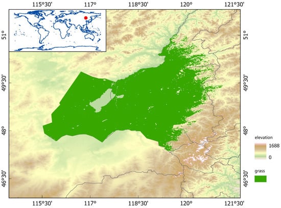
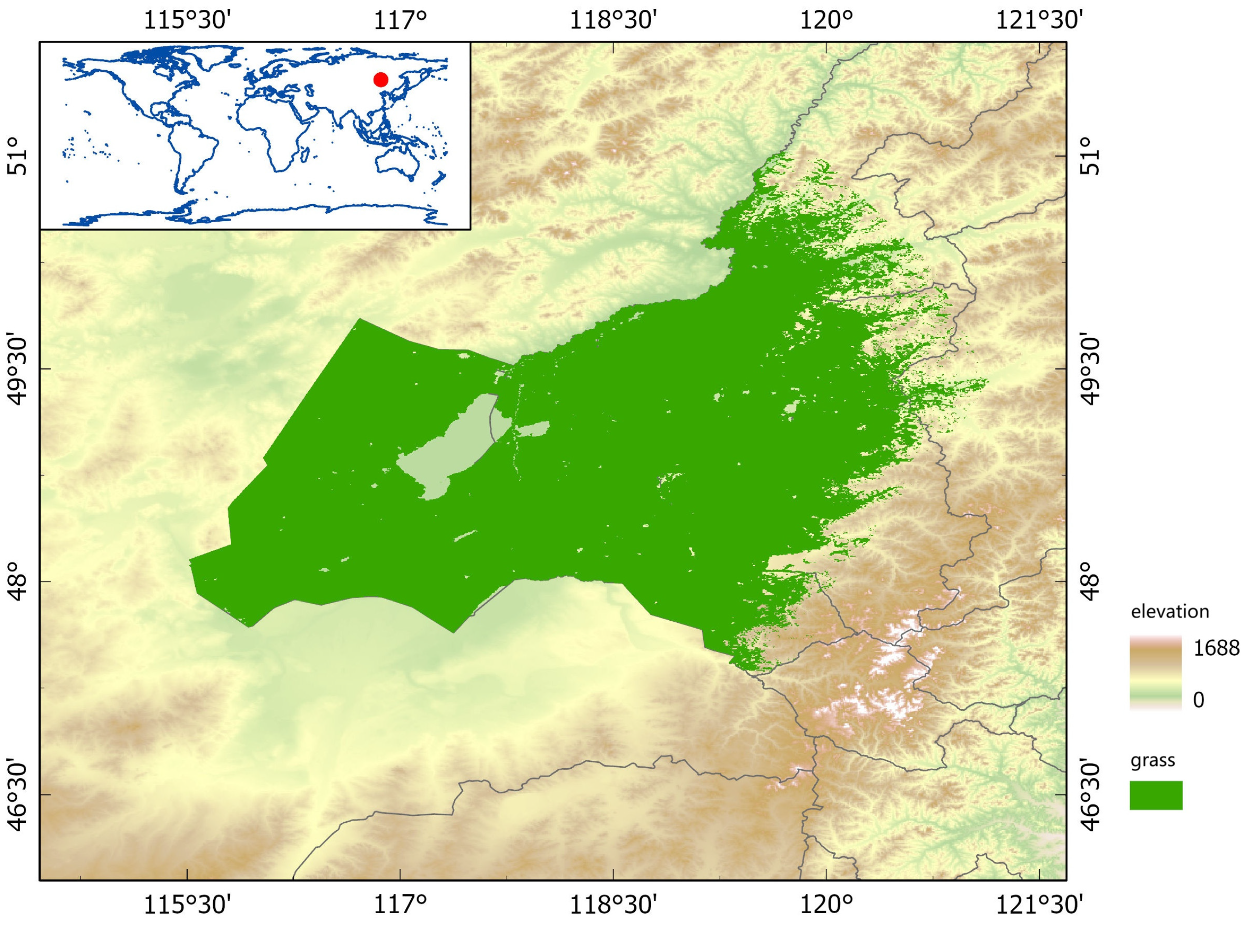
This study focuses on the Hulunbuir grassland located on the western side of the Greater Khingan Mountains (Figure 1), covering 46.94–51.13° N and 115.31–123.68° E, with a total area of approximately 110,500 km². The terrain gradually rises from west to east, with elevations increasing from about 600 m on the western plateau to nearly 1500 m along the eastern mountain ridges. The study area has a typical temperate semi-arid continental climate, characterized by long, cold winters and short, warm summers. The annual mean temperature ranges from −2 °C to 2 °C. Influenced by the topographic barrier of the Greater Khingan Mountains and the East Asian monsoon circulation, annual precipitation ranges from 300 to 500 mm and exhibits a pronounced decreasing gradient from east to west. Moreover, precipitation is highly unevenly distributed throughout the year, with approximately 70% occurring during July and August. These pronounced climatic gradients provide a natural setting for investigating the responses of NDVI to meteorological drivers.

Figure 1. Location of the study area (Hulunbuir Grassland), indicated by the red dot.

Driven by the spatial variation in hydrothermal conditions, the study area exhibits a vegetation transition from meadow steppe to typical steppe. The dominant vegetation types include meadow steppe, typical steppe, and sparse sandy vegetation. Soil development is also spatially differentiated, with chernozem soils predominating in the eastern region and chestnut soils becoming increasingly common toward the west. As one of China’s major high-quality forage production bases and an important ecological barrier, the vegetation dynamics of the Hulunbuir grassland are closely associated with the sustainable development of regional animal husbandry and ecological security.

2.2. Basic Data

This study obtained four types of fundamental datasets, including land cover, Normalized Difference Vegetation Index (NDVI), temperature, and precipitation, from the Google Earth Engine (GEE) platform. All original datasets were subjected to consistent preprocessing procedures to provide the data foundation for constructing the pixel-level temporal prediction model.

The land cover data were obtained from the MODIS MCD12Q1 dataset, covering the period from 2013 to 2024 with a spatial resolution of 1000 m. For each year within the study period, grassland pixels were extracted from the land cover maps. Subsequently, a pixel-wise annual logical “OR” operation was applied to generate the maximum grassland extent dataset during 2013–2024, which was used to define the spatial extent of the study area and the valid pixels for subsequent NDVI and meteorological data analysis. This unified grassland extent was used as the spatial mask to ensure consistent spatial coverage among the datasets.

The NDVI data were derived from the MODIS MOD13A1 dataset, which provides a 16-day Maximum Value Composite (MVC) product with a spatial resolution of 1000 m. In this study, the MOD13A1 data were further composited on a monthly basis using the maximum value method, resulting in a monthly NDVI time series dataset from 2013 to 2024, consisting of 144 months with a spatial resolution of 1000 m.

The meteorological data included 2 m air temperature (temperature_2m) and total precipitation (total_precipitation_sum), both obtained from the ERA5-Land dataset with a spatial resolution of 1000 m and covering the period from 2013 to 2024. Monthly temperature time series were generated by calculating the monthly mean values, while monthly precipitation time series were obtained by accumulating daily precipitation values within each month. Both meteorological variables were processed to match the temporal and spatial scales of the NDVI dataset. All datasets were spatially aligned to the same 1000 m grid and clipped using the unified grassland mask.

During data preprocessing, background and invalid raster values, including NoData values, were identified and excluded using the valid-pixel mask. Only pixels with valid data were retained for subsequent model construction. This procedure ensured that the meteorological inputs and NDVI prediction targets were aligned at the pixel level and prevented invalid observations from entering the model.

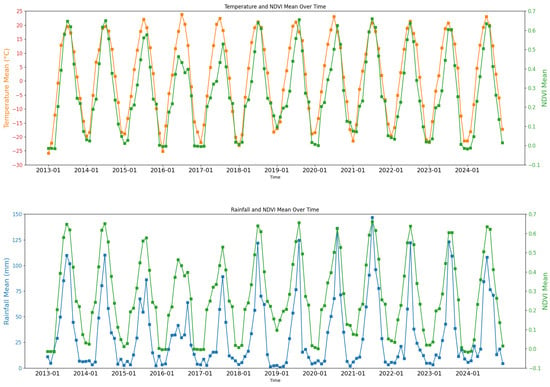
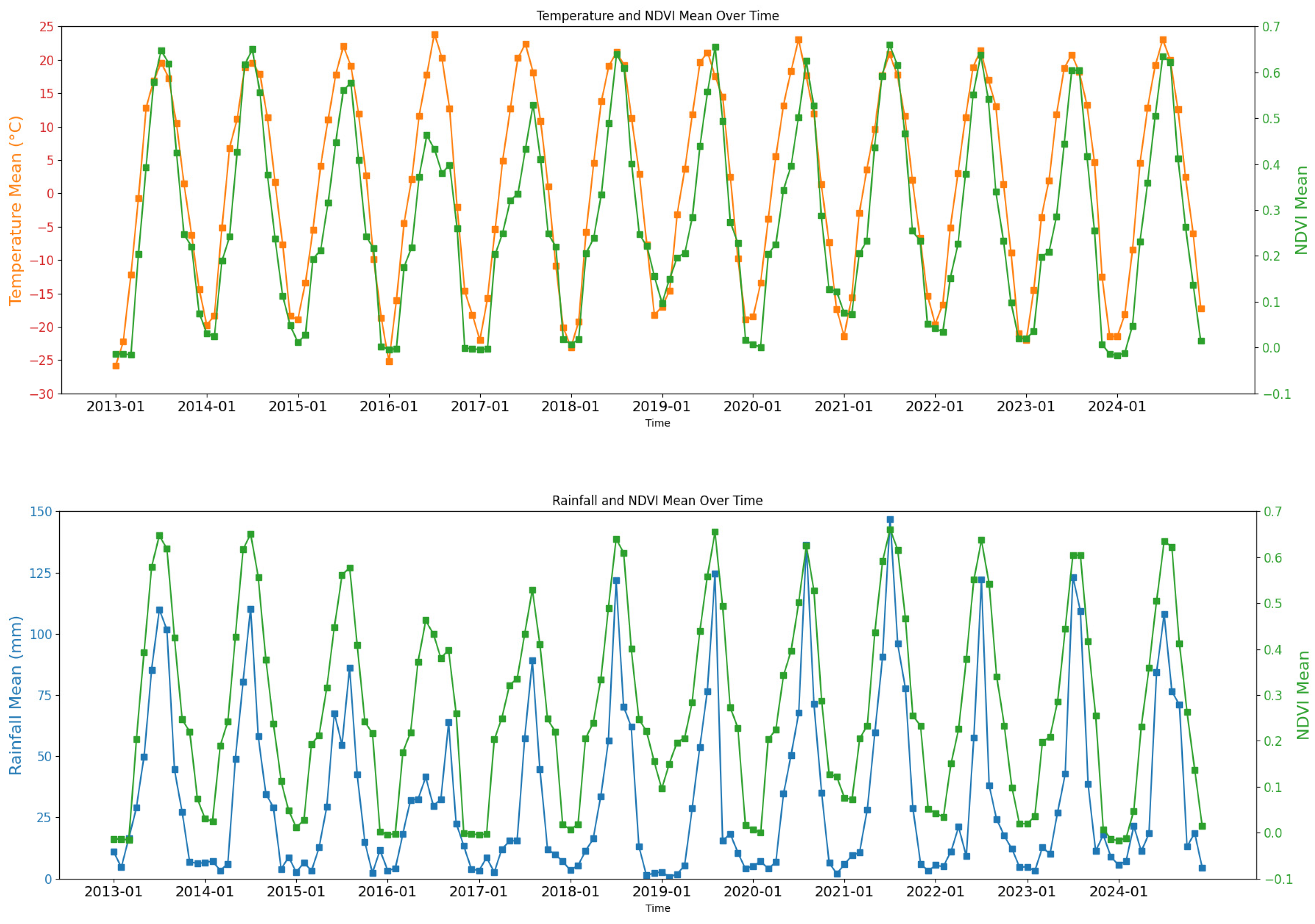
All four datasets were raster products with a spatial resolution of 1000 m. For preliminary temporal analysis and visualization, spatial averaging was performed over the valid pixels within the study area to characterize the overall monthly variations in NDVI, temperature, and precipitation from 2013 to 2024 (Figure 2). These regional mean time series were used exclusively for descriptive analysis and visualization and were not used as model inputs or training samples. In contrast, DfT-Net was trained using the original pixel-level 1000 m data, with each valid grassland pixel treated as an independent prediction unit. The same model parameters were shared across pixels, allowing the model to learn common meteorological–vegetation response patterns while generating predictions that could be mapped back to their corresponding spatial locations. The multi-year mean temperature, precipitation, and NDVI values were 1.46 ± 14.82 °C, 32.69 ± 34.90 mm, and 0.2756 ± 0.2060, respectively.

Figure 2. Monthly time series of NDVI, temperature, and precipitation in the Hulunbuir grassland during 2013–2024.

The peaks and troughs of the three variables showed recurrent temporal distributions over multiple years. The maximum values generally occurred during summer (July–August), whereas the minimum values mainly appeared during winter (November to February of the following year), indicating a stable annual cyclic structure between climatic conditions and vegetation growth processes in the study area. From the perspective of time series characteristics, the continuous monthly observations during 2013–2024 exhibited clear periodic repetition, with similar variation patterns occurring in the same months across different years. This recurring temporal structure can be interpreted as a form of temporal symmetry, in which the system exhibits similar seasonal responses under recurring annual climatic forcing.

Specifically, temperature variations mainly represent the annual thermal cycle, precipitation variations reflect seasonal water availability regulation, and NDVI variations integrate the effects of temperature and moisture conditions to characterize vegetation growth cycles. This periodic structure provides the data basis for subsequent extraction of trend, seasonal, and residual components using time series decomposition methods. It also highlights the necessity of incorporating temporal characteristics into model construction to improve NDVI prediction accuracy.

2.3. Methodology

2.3.1. Overall Technical Framework

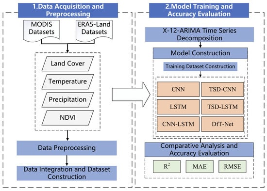
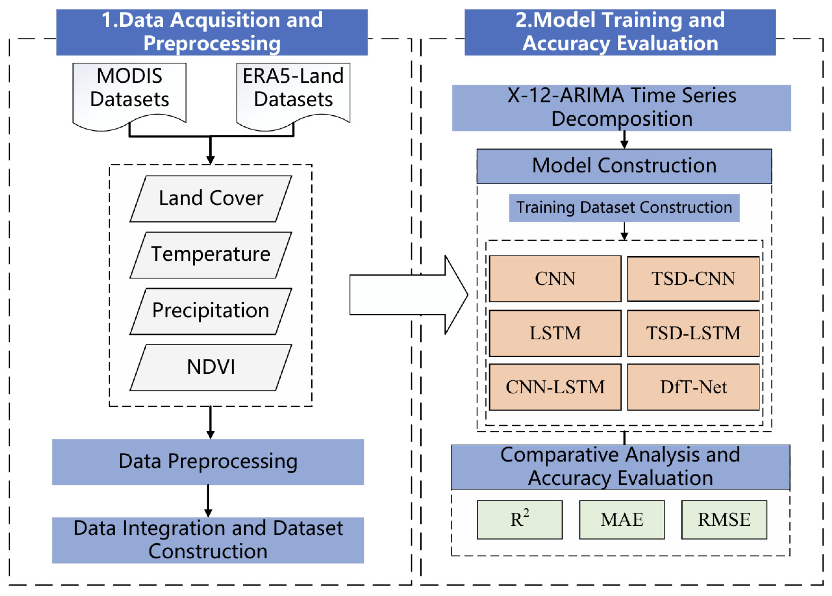
The overall technical framework of this study is illustrated in Figure 3, which mainly consists of the following four steps:

Figure 3. Technical framework of this study.

(1)

Data acquisition and preprocessing.

NDVI, precipitation, and temperature data for the Hulunbuir grassland during 2013–2024 were obtained from the Google Earth Engine (GEE) platform. The original datasets were preprocessed through spatial clipping, temporal scale harmonization, and missing data processing to construct a basic dataset with consistent spatial coverage, temporal periods, and spatial and temporal resolutions.

(2)

Time series decomposition of meteorological data.

The X-12-ARIMA method was applied to decompose the time series of the two meteorological variables (temperature and precipitation) into three components: trend, seasonal, and residual components. This decomposition enabled the extraction of temporal variation characteristics at different scales and provided multi-level meteorological driving factors for model construction. Although NDVI was also decomposed during the preliminary temporal analysis to investigate its temporal characteristics, the decomposed NDVI components were not used as model inputs or training features. The original pixel-level NDVI was directly used as the prediction target.

(3)

Model construction, training, and NDVI prediction.

Considering the influence of time series decomposition, the original and decomposed meteorological sequences were separately integrated with independent CNN, LSTM, and CNN-LSTM models, resulting in six experimental schemes. The proposed DfT-Net integrates the decomposed temperature and precipitation features with CNN and LSTM to jointly characterize local temporal patterns and long-term temporal dependencies. All models were trained using valid pixel-level samples, with the same model architecture and parameters applied across pixels. These schemes were used for model training and NDVI prediction, and the performance differences among various approaches were systematically compared.

(4)

Model evaluation and key factor analysis.

The prediction performance of the six experimental schemes was evaluated using statistical metrics, including the coefficient of determination (R²), root mean square error (RMSE), and mean absolute error (MAE). Furthermore, the impacts of meteorological factor decomposition, model architecture, and temporal feature representation on prediction accuracy were analyzed to identify the key factors contributing to improved NDVI prediction performance.

2.3.2. Time Series Decomposition (TSD)

As shown in Figure 2, temperature, precipitation, and NDVI in the study area exhibit distinct seasonal variation characteristics and annual cyclic patterns. Meanwhile, at the long-term scale from 2013 to 2024, no obvious overall trends were observed in temperature and precipitation. Since vegetation growth is strongly regulated by seasonal climatic conditions, meteorological variables and NDVI time series generally contain stable periodic repetition structures, where similar variation patterns occur at corresponding time intervals across different years. This phenomenon, referred to as temporal symmetry induced by seasonal cycles, reflects the response mechanisms of ecosystems to periodic environmental changes.

However, raw time series usually contain multiple components, including long-term trends, periodic fluctuations, and random disturbances. Directly inputting these mixed signals into prediction models may result in interference among information at different temporal scales. Therefore, to effectively extract periodic structures and latent patterns from time series data while reducing the influence of random noise during model training, this study applied Time Series Decomposition (TSD) to the non-stationary temperature and precipitation sequences. The original time series were decomposed into three components: trend, seasonal, and residual components.

The time series decomposition can be expressed as follows:

$$Y_i=T_i+S_i+R_i,$$

(1)

where $Y_i$ represents the original time series, and $T_i$, $S_i$, and $R_i$ denote the trend, seasonal, and residual components of the time series at time step $i$, respectively.

In this study, the X-12-ARIMA method was employed for time series decomposition. Proposed by the U.S. Census Bureau, X-12-ARIMA integrates the advantages of ARIMA modeling and the X-11 moving average method and has been widely applied in environmental time series analysis [23,24,25,26]. The method consists of three core modules: RegARIMA pre-adjustment, X-12 seasonal adjustment, and diagnostic and validation modules, enabling accurate time series decomposition through a multi-stage processing framework. The ARIMA model converts non-stationary time series into stationary sequences through differencing techniques [27] and characterizes temporal dependencies using autoregressive (AR) and moving average (MA) components [28].

The X-12-ARIMA method was selected based on the characteristics of the meteorological data and the objectives of this study. First, temperature and precipitation were represented as monthly time series with pronounced and recurrent seasonal patterns. X-12-ARIMA is specifically designed for seasonal time-series analysis and is therefore suitable for separating systematic seasonal variation from long-term and irregular components. Second, the combination of RegARIMA modeling and moving-average-based seasonal adjustment enables the method to account for both temporal dependence and seasonal structure, which is appropriate for meteorological sequences characterized by strong seasonality and interannual variability. Third, the resulting trend, seasonal, and residual components have clear temporal interpretations and can be directly incorporated as multi-scale meteorological features into the prediction model. Therefore, X-12-ARIMA was considered an appropriate and interpretable decomposition method for extracting the multi-scale temporal characteristics of temperature and precipitation in this study.

For model construction, X-12-ARIMA was independently applied to the monthly temperature and precipitation sequences of each valid 1000 m grassland pixel from 2013 to 2024, resulting in 144 monthly observations for each variable. Each pixel-level meteorological sequence was decomposed into trend, seasonal, and residual components. Accordingly, six decomposed meteorological sequences were obtained for each pixel and used as the input features of DfT-Net. The original pixel-level NDVI was directly used as the prediction target and was not decomposed for model training.

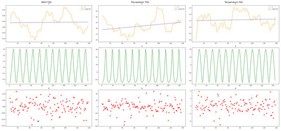
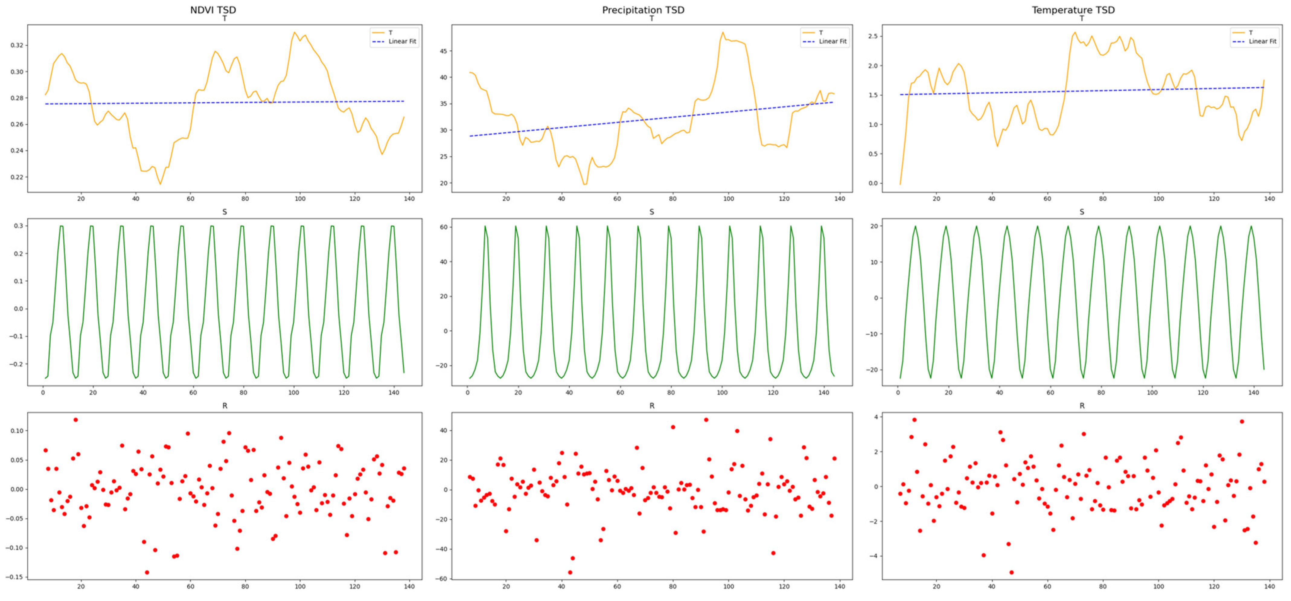
For preliminary temporal analysis, TSD was additionally applied to the regional mean temperature, precipitation, and NDVI time series to characterize their overall trend, seasonal, and residual components, as shown in Figure 4. These regional decomposition results were used exclusively for descriptive analysis and visualization and were not involved in model training or prediction. In particular, the NDVI decomposition was conducted only to examine its temporal characteristics and seasonal structure; no decomposed NDVI component was used as a model input or training feature. The ranges of the trend components for temperature, precipitation, and NDVI were 1.487 ± 1.155 °C, 32.827 ± 9.830 mm, and 0.2758 ± 0.064, respectively. The seasonal components exhibited ranges of 0 ± 14.716 °C, 0 ± 31.211 mm, and 0 ± 0.206, respectively. The residual components fluctuated within ranges of −0.02 ± 1.724 °C, −0.137 ± 18.160 mm, and 0 ± 0.071, respectively.

Figure 4. Time series decomposition results of the datasets.

Trend analysis indicated that neither NDVI nor temperature exhibited significant increasing or decreasing trends during the 12-year study period, although both showed certain fluctuations. In contrast, precipitation demonstrated a significant increasing trend (p = 0.0009). The decomposition results indicate that the seasonal components effectively preserved the periodic repetition information contained in temperature, precipitation, and NDVI variations. These results provide a basis for understanding the temporal characteristics and seasonal symmetry of vegetation–climate interactions, while the pixel-level decomposition of temperature and precipitation provides the meteorological input features for subsequent DfT-Net training.

2.3.3. Prediction Model Construction

(1)

CNN

A one-dimensional convolutional neural network (CNN) is a deep learning model capable of effectively extracting local variation features from time series data. Although conventional CNNs are primarily designed for spatially structured data such as images, one-dimensional convolutional networks are also suitable for time series analysis due to their local receptive fields and parameter-sharing characteristics [29]. A typical CNN architecture generally consists of convolutional layers, batch normalization layers, pooling layers, and fully connected layers.

The convolutional layer performs sliding operations on the input sequence using multiple convolution kernels to extract variation patterns within local temporal windows. Since the same convolution kernel parameters are shared across different temporal positions, this process exhibits a certain degree of temporal translation equivariance, meaning that sequence segments with similar variation patterns occurring at different time points can be consistently extracted through shared parameters. This mechanism is consistent with the recurrent variation patterns observed at the same seasonal stages across different years during vegetation growth, thereby facilitating the learning of local periodic structures embedded in time series data.

The batch normalization layer standardizes intermediate feature representations to improve training stability and accelerate convergence. The pooling layer reduces data dimensionality through feature compression, retaining essential variation information while minimizing redundant features. Finally, the fully connected layer integrates the high-dimensional features extracted by convolutional operations to generate prediction outputs.

In this study, two independent Conv1D networks were constructed using temperature and precipitation sequences, respectively. The convolution kernel size was set to 3 to capture short-term local variation characteristics of meteorological factors. The models were trained with a learning rate of 0.0001, and optimal performance was achieved by adjusting training parameters such as the number of epochs.

(2)

LSTM

The Long Short-Term Memory network (LSTM) is an improved recurrent neural network (RNN) architecture that enhances long-term information propagation through the introduction of gating mechanisms, effectively alleviating the problems of gradient vanishing and gradient explosion commonly encountered in conventional RNNs [30].

An LSTM network mainly consists of three gates: the input gate, forget gate, and output gate. By controlling the retention, updating, and output of historical information, LSTM can effectively model long-term dependencies within time series data [31,32]. For ecological time series characterized by pronounced seasonal cycles, LSTM can learn interannual evolutionary relationships over long temporal scales and capture dynamic interactions between climatic drivers and vegetation responses.

From the perspective of temporal symmetry, vegetation NDVI and meteorological variables generally exhibit recurrent seasonal variation patterns across years. Through its recurrent state transition mechanism, LSTM is capable of preserving such long-term evolutionary information and identifying latent correlations among different temporal cycles.

In this study, LSTM networks were constructed for six categories of decomposed temporal features, including the trend, seasonal, and residual components derived from temperature and precipitation time series. Each feature component was input into an independent LSTM layer, and network parameters were optimized to achieve the best prediction performance.

(3)

CNN-LSTM Hybrid Model

Considering the complementary advantages of CNN and LSTM in feature learning, a CNN-LSTM hybrid model was further developed to simultaneously extract local variation characteristics and long-term temporal dependencies from time series data.

The CNN component first performs convolution operations on the input meteorological sequences. Through parameter-sharing mechanisms, CNN extracts local variation patterns with similar characteristics across different temporal windows and enhances the model’s ability to recognize local temporal structures. Subsequently, the feature sequences generated by CNN are used as inputs to LSTM, which further learns long-term temporal dependencies through recurrent connections and captures cross-cycle dynamic response characteristics during vegetation evolution.

The hybrid model combines the local feature extraction capability of CNN with the long-term sequence modeling capability of LSTM, enabling joint modeling of vegetation dynamics driven by meteorological factors. Specifically, CNN focuses on extracting locally repeated structures within time series, whereas LSTM establishes long-term evolutionary relationships. Their integration improves the model’s ability to characterize periodic NDVI variation patterns.

In this study, the CNN-LSTM model was constructed by sequentially connecting Conv1D layers and LSTM layers, and model performance was optimized by adjusting network hyperparameters.

(4)

Dual-Factor-Driven Temporal Network (DfT-Net)

To integrate the complementary information provided by temperature and precipitation while preserving the temporal characteristics of meteorological drivers, a dual-factor-driven temporal network (DfT-Net) was developed for spatially distributed pixel-level NDVI prediction. The proposed model integrates dual-factor meteorological driving information, time series decomposition, local temporal feature extraction, and long-term temporal dependency modeling within a unified prediction framework.

For spatially distributed prediction, the study area was represented by valid 1000 m grassland pixels. Each valid pixel was treated as an independent prediction unit, and the corresponding temperature, precipitation, and NDVI observations were organized as pixel-level time series. The same DfT-Net architecture and model parameters were shared across all valid pixels. Consequently, model training was performed using temporal samples from spatially distributed pixels rather than a regional-average time series. After prediction, the outputs of individual pixels were assigned back to their original geographic locations, allowing the predicted NDVI values to be reconstructed as spatially distributed prediction maps.

The temporal dimension was explicitly modeled using decomposed temperature and precipitation sequences. For each valid pixel, the temperature and precipitation time series were independently decomposed into trend, seasonal, and residual components using X-12-ARIMA. The resulting six meteorological features were subsequently processed through the corresponding neural network layers. Conv1D was used to extract local temporal variation patterns, whereas LSTM was used to capture long-term temporal dependencies and recurrent relationships across seasonal and interannual cycles. The six decomposed meteorological features were jointly incorporated into the prediction process to characterize the temporal response of vegetation to thermal and moisture conditions.

From the perspective of temporal symmetry, the seasonal components obtained through TSD preserve the recurrent variation structures of temperature and precipitation across successive annual cycles. Meanwhile, the parameter-sharing mechanism of Conv1D enables similar local temporal patterns to be recognized at different positions along the time axis. LSTM further captures long-term dependencies among recurrent seasonal and interannual cycles. Through the combination of these mechanisms, DfT-Net exploits the periodic temporal structure of meteorological drivers and their relationships with NDVI dynamics.

The spatial distribution of the predictions does not represent explicit spatial dependency modeling. The model does not perform convolution, attention, or other operations between neighboring pixels and therefore does not explicitly learn spatial correlations among adjacent pixels. Instead, each valid pixel is independently modeled using its own meteorological and NDVI time series, while the shared model parameters allow common meteorological–vegetation response patterns to be learned across spatially distributed pixels. Therefore, DfT-Net should be regarded as a temporal prediction framework applied independently across spatially distributed pixels, rather than as an explicit spatio-temporal model.

2.3.4. Dataset Partitioning

In this study, the dataset covering the period from 2013 to 2024 (a total of 12 years) was divided into training, validation, and testing sets at a ratio of 8:1:3. Specifically, data from the first eight years were used for model training, data from the ninth year were used for validation, and data from the final three years were reserved for independent testing and performance evaluation. This chronological division was adopted to avoid information leakage from future observations and to provide a more realistic assessment of the model’s forecasting capability. The final three years were selected as an independent testing period to evaluate the model under unseen future temporal conditions.

Furthermore, considering different deep learning model architectures and whether Time Series Decomposition (TSD) preprocessing was applied, six experimental cases were designed and comparatively evaluated, including CNN, TSD-CNN, LSTM, TSD-LSTM, CNN-LSTM, and DfT-Net, as presented in Table 1. These experiments were conducted to investigate the effects of time series decomposition and model structure on NDVI prediction performance.

Table 1. Experimental configurations of multiple prediction models considering TSD preprocessing.

Model	TSD Preprocessing
CNN	No
LSTM	No
CNN-LSTM	No
TSD-CNN	Yes
TSD-LSTM	Yes
DfT-Net	Yes

2.3.5. Model Performance Evaluation

The predictive performance of the proposed models was evaluated using three commonly adopted statistical metrics: the Root Mean Square Error (RMSE), Mean Absolute Error (MAE), and the coefficient of determination (R²). The corresponding formulations are given as follows:

$$RMSE=\sqrt{{\displaystyle \frac{1}{n}}{\displaystyle {\sum }_{i=1}^n}{(y_i-\widehat{y_i})}^2},$$

(2)

$$MAE={\displaystyle \frac{1}{n}}{\displaystyle {\sum }_{i=1}^n}\left|y_i-\widehat{y_i}\right|,$$

(3)

$$R^2={\displaystyle \frac{{\left({\displaystyle {\sum }_{i=1}^n}(y_i-\overline{y_i})\left(x_i-\overline{x_i}\right)\right)}^2}{{\displaystyle {\sum }_{i=1}^n}{(y_i-\overline{y_i})}^2{\left(x_i-\overline{x_i}\right)}^2}},$$

(4)

where $n$ denotes the number of samples, $y_i$ is the observed NDVI value of the i-th sample, and ${\widehat{y}}_i$ is the corresponding predicted value. $\overline{y}$ and $\overline{\widehat{y}}$ represent the mean values of the observed and predicted NDVI, respectively.

Lower values of RMSE and MAE indicate higher prediction accuracy, whereas an R² value closer to 1 indicates better agreement between the predicted and observed values and thus superior model performance.

3. Results

3.1. Visual Assessment

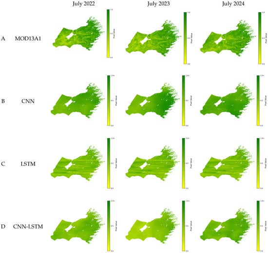
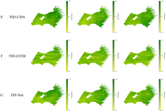
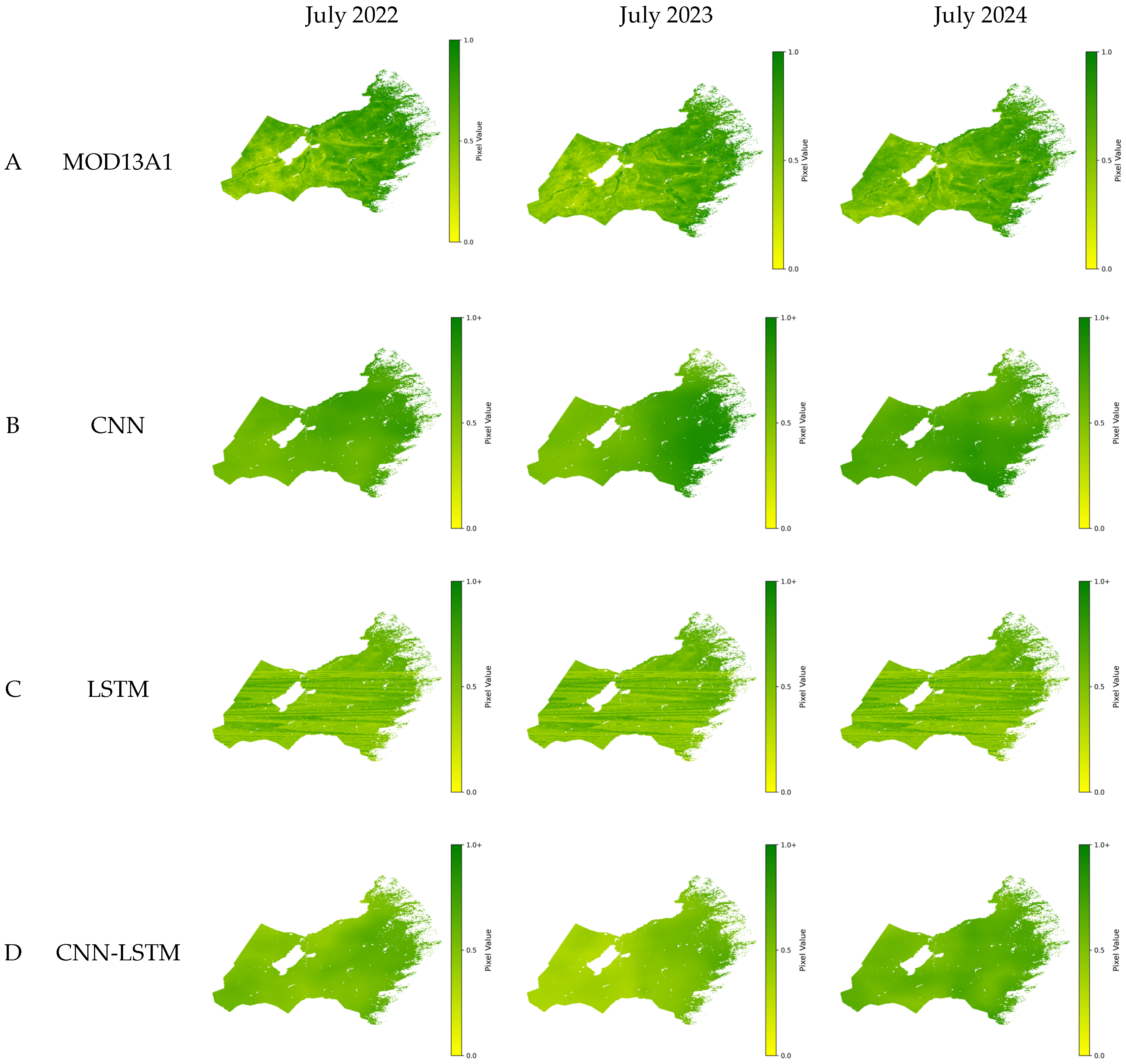
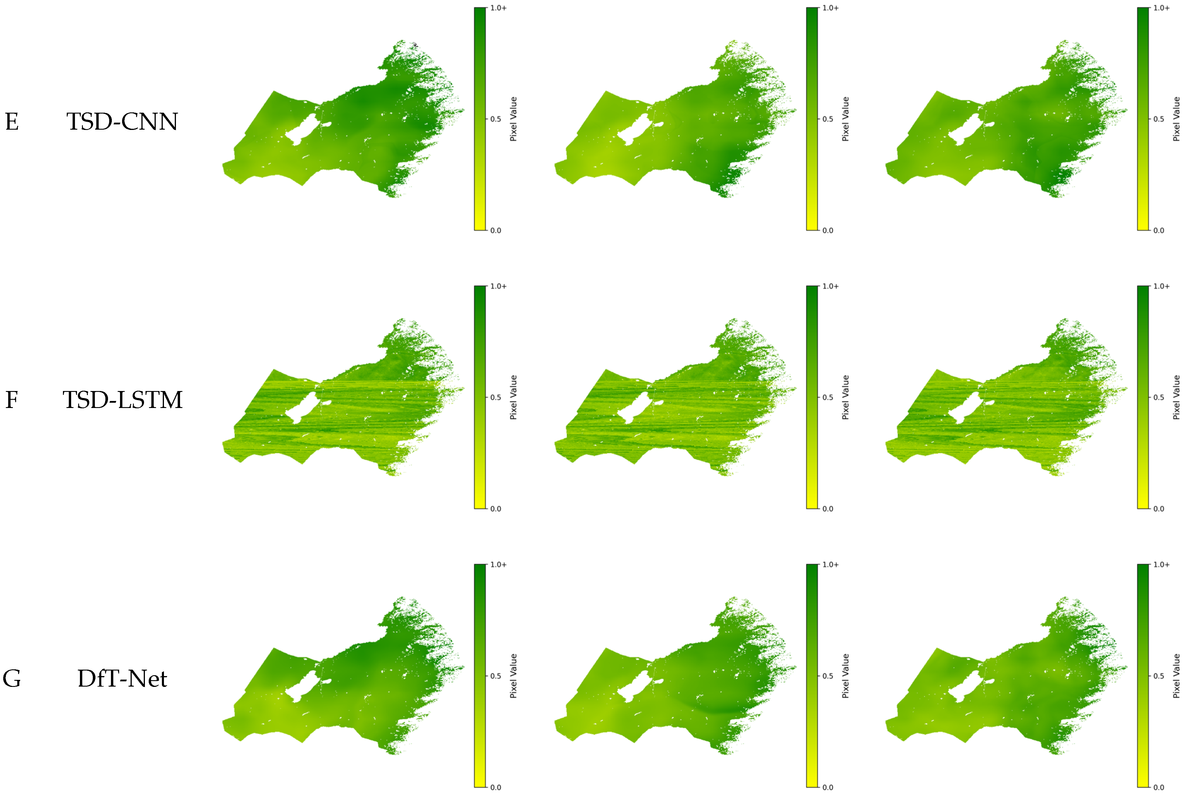
During the peak growing season of grassland vegetation (July), the NDVI prediction results of the six models across the study area are shown in Figure 5. Overall, all six models successfully captured the spatial distribution pattern of pixel-level NDVI predictions, characterized by a gradual decrease from east to west and from south to north. This spatial distribution pattern was consistent with the observed NDVI distribution (Figure 5A), indicating that the pixel-level prediction framework was able to preserve the geographic distribution of predicted NDVI values.

Figure 5. MODIS NDVI and prediction results of different models during the peak growing season of grassland vegetation (July).

A detailed examination of the spatially mapped prediction results showed that the transition zone from meadow steppe to typical dry steppe along the western foothills of the Greater Khingan Mountains exhibited a rapid NDVI gradient. In this region, the DfT-Net model demonstrated relatively better consistency with the observed NDVI distribution, suggesting that its combined modeling of decomposed meteorological features and temporal dependencies may improve the prediction of vegetation variation across individual pixels. However, this spatial pattern does not indicate that DfT-Net explicitly learns spatial relationships among neighboring pixels, as each pixel is treated as an independent prediction unit.

3.2. Bias Analysis

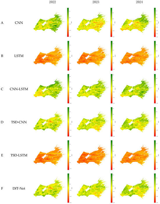
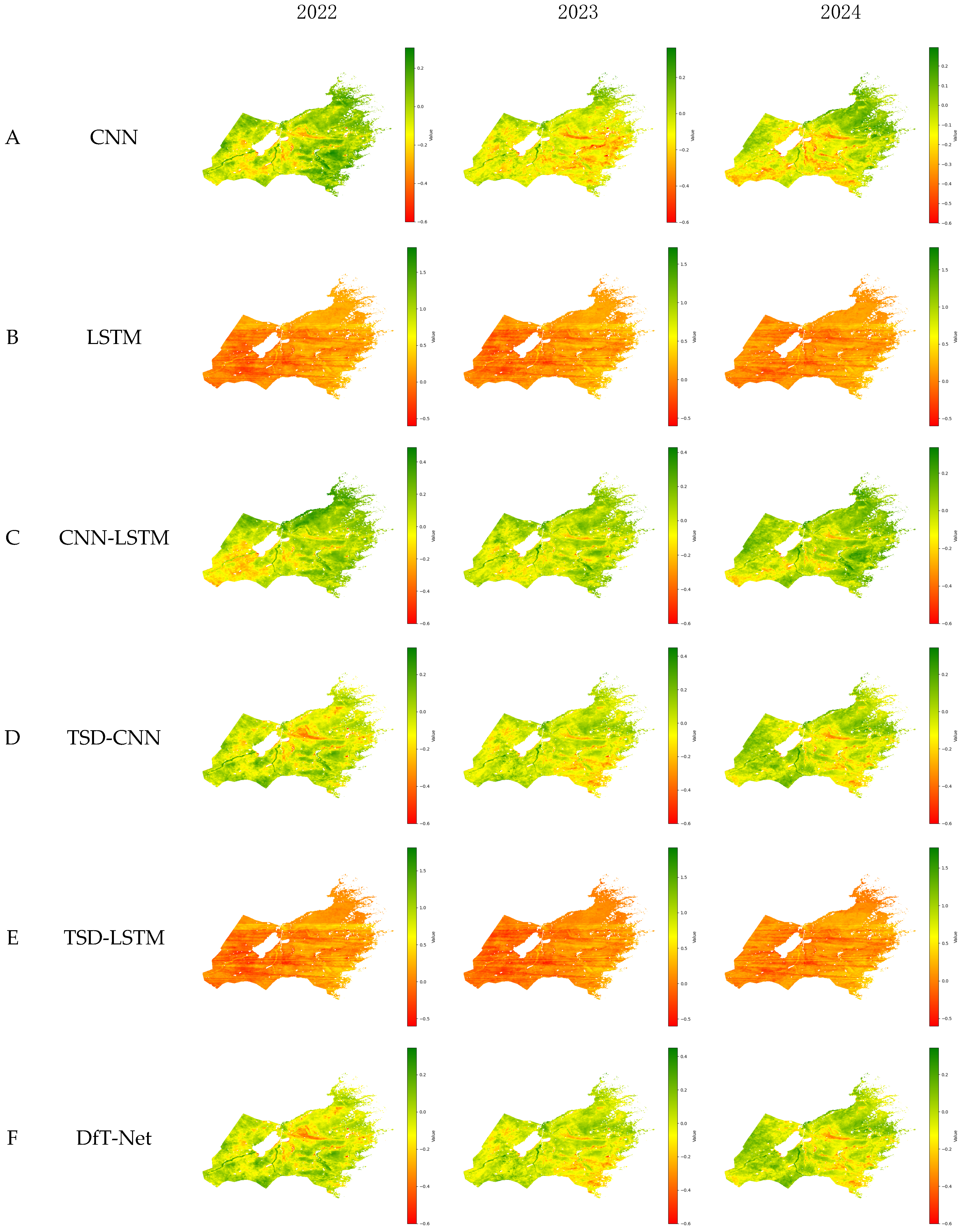
The prediction results of the six models obtained in Figure 5 (Figure 5B–G) were subtracted from the observed MODIS NDVI values (Figure 5A) to calculate the prediction errors between each model and the reference NDVI. The spatial distributions of these differences are presented in Figure 6.

Figure 6. Spatial differences between the NDVI predictions of different models and the MODIS NDVI (MOD13A1) during the peak growing season of grassland vegetation (July).

The results clearly show that, in July, the prediction errors of almost all models were closest to zero in the central region of the study area. Meanwhile, negative biases dominated most areas, indicating that the predicted NDVI values from all models were generally higher than the observed values. In contrast, positive biases were mainly distributed in the marginal areas, particularly in the northeastern and northern regions, suggesting that model predictions tended to underestimate NDVI values in these areas.

The models based solely on LSTM (Figure 5B,F) exhibited an overall underestimation tendency across the study area. In comparison, the other four models incorporating CNN structures did not show apparent systematic overestimation or underestimation. Instead, their positive and negative biases exhibited a more random spatial distribution pattern.

3.3. Overall Evaluation of Model Performance

The prediction results across the entire study area exhibited variation patterns similar to those of the observed NDVI values. Since the evaluation based on a single month cannot fully represent the overall predictive capability of a model, the six models were assessed using data from all 12 months and the entire study area. The evaluation results are presented in Table 2.

Table 2. Performance evaluation of different models.

Year	Model	RMSE	R2	MAE
2022	TSD-CNN	0.103	0.811	0.072
	TSD-LSTM	0.132	0.680	0.121
	CNN-LSTM	0.134	0.704	0.100
	CNN	0.104	0.817	0.076
	LSTM	0.158	0.560	0.121
	DfT-Net	0.103	0.823	0.078
2023	TSD-CNN	0.103	0.837	0.074
	TSD-LSTM	0.130	0.700	0.098
	CNN-LSTM	0.119	0.811	0.093
	CNN	0.108	0.832	0.083
	LSTM	0.116	0.565	0.133
	DfT-Net	0.101	0.833	0.093
2024	TSD-CNN	0.129	0.808	0.100
	TSD-LSTM	0.137	0.706	0.105
	CNN-LSTM	0.107	0.832	0.083
	CNN	0.127	0.809	0.101
	LSTM	0.166	0.565	0.133
	DfT-Net	0.099	0.852	0.071
2022–2024	TSD-CNN	0.112	0.808	0.082
	TSD-LSTM	0.133	0.694	0.100
	CNN-LSTM	0.120	0.753	0.092
	CNN	0.114	0.804	0.087
	LSTM	0.157	0.572	0.124
	DfT-Net	0.100	0.828	0.074

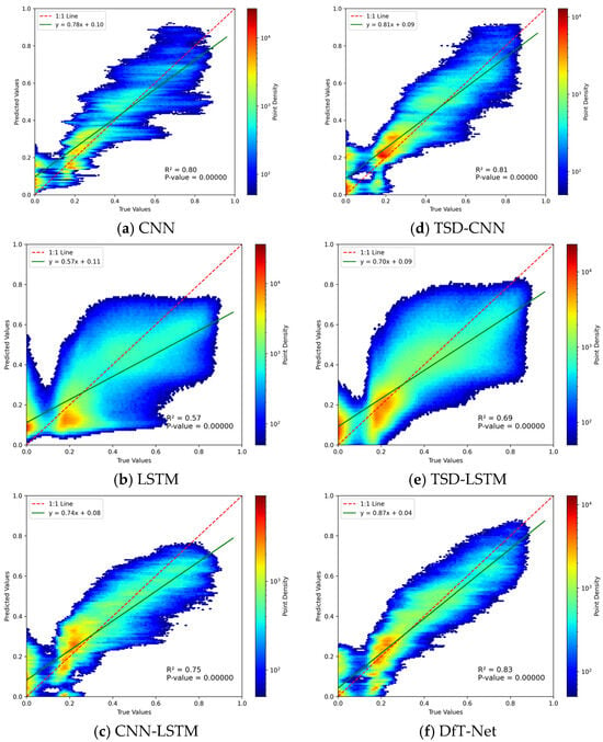
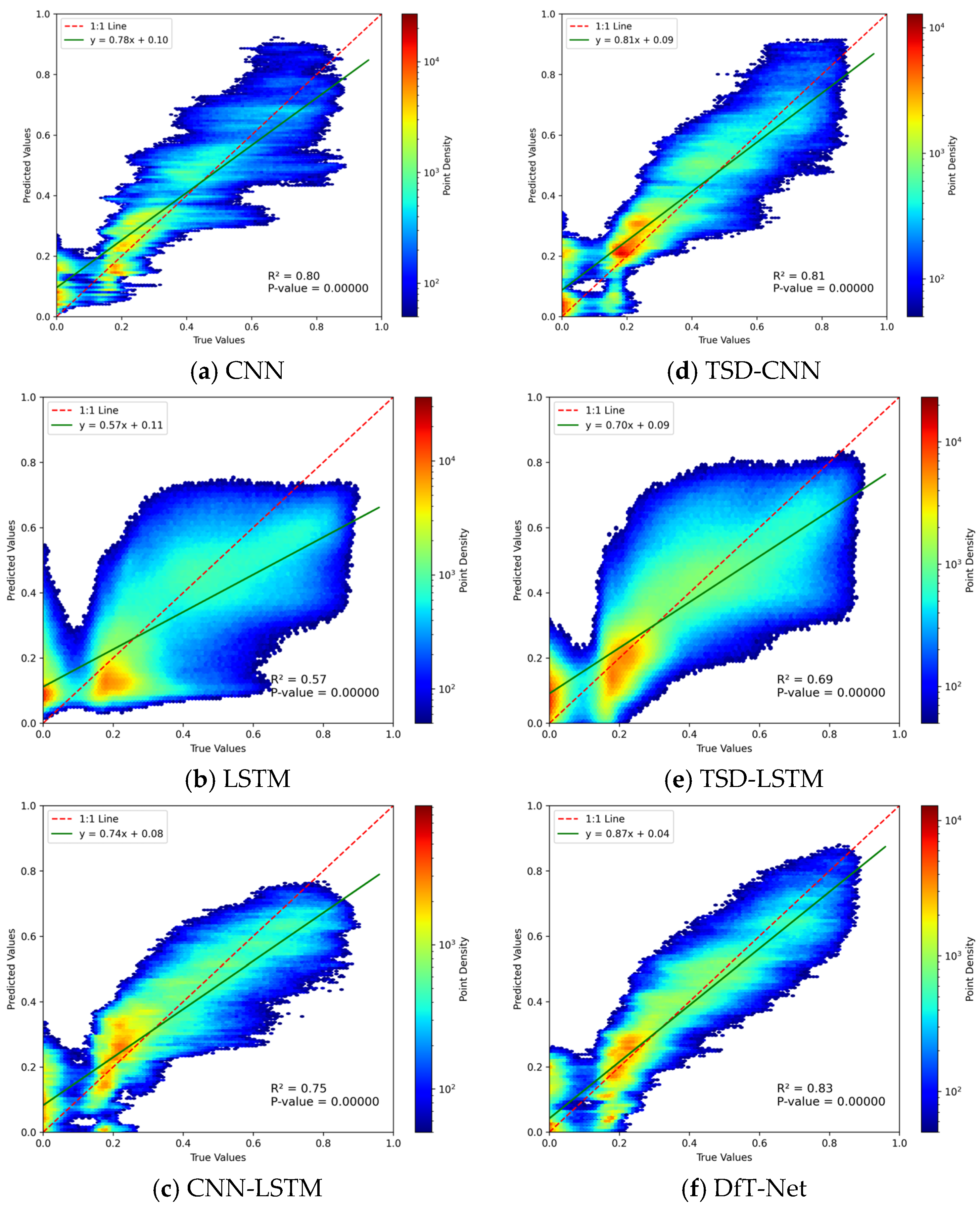
A linear regression analysis between the predicted and observed NDVI values was conducted using all prediction samples from the study area over the 36-month testing period, and the corresponding scatter plots are shown in Figure 7. The first row of Figure 7 presents the results without Time Series Decomposition (TSD) preprocessing, whereas the second row shows the results after TSD preprocessing. From left to right, the models are arranged as CNN, LSTM, and CNN-LSTM.

Figure 7. Density scatter plots between NDVI predictions from different models and MODIS NDVI.

Due to the large number of samples, point density was used to represent the distribution characteristics in the scatter plots. Red indicates densely distributed sample points, whereas blue represents relatively sparse point distributions (with a minimum density value of 50). The green solid line represents the fitted linear regression equation, and the red dashed line denotes the one-to-one reference line where predicted values are equal to observed values.

The results clearly demonstrate that among the six models, the LSTM-based models exhibited more dispersed point distributions and achieved the lowest prediction accuracy. In contrast, the other four models showed relatively better predictive performance, with most sample points concentrated near the one-to-one reference line, indicating stronger agreement between predicted and observed NDVI values.

By comparing models with and without Time Series Decomposition (TSD) preprocessing, it was observed that models trained using TSD-processed data achieved higher prediction accuracy. Furthermore, when comparing models based solely on CNN or LSTM architectures, the LSTM-based models showed lower accuracy than CNN-based models. By integrating CNN and LSTM, the hybrid model combined the advantages of both architectures and achieved better performance than the models using a single network. Although the overall three-year prediction performance of CNN-LSTM was slightly lower than that of CNN, it achieved relatively high accuracy in 2023 and 2024, with R² values exceeding 0.8.

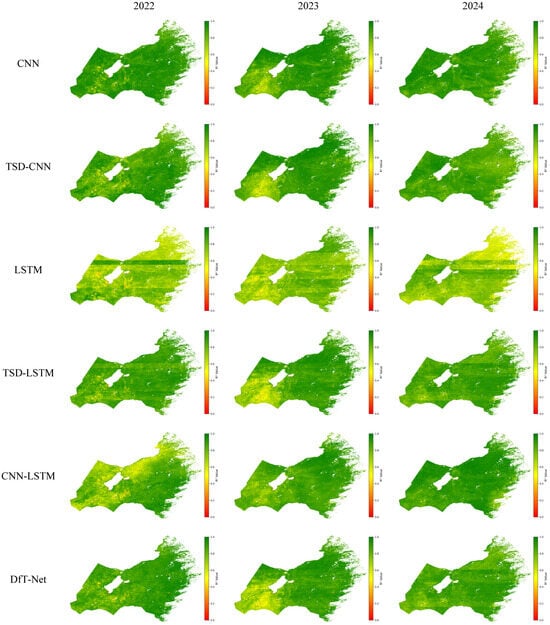
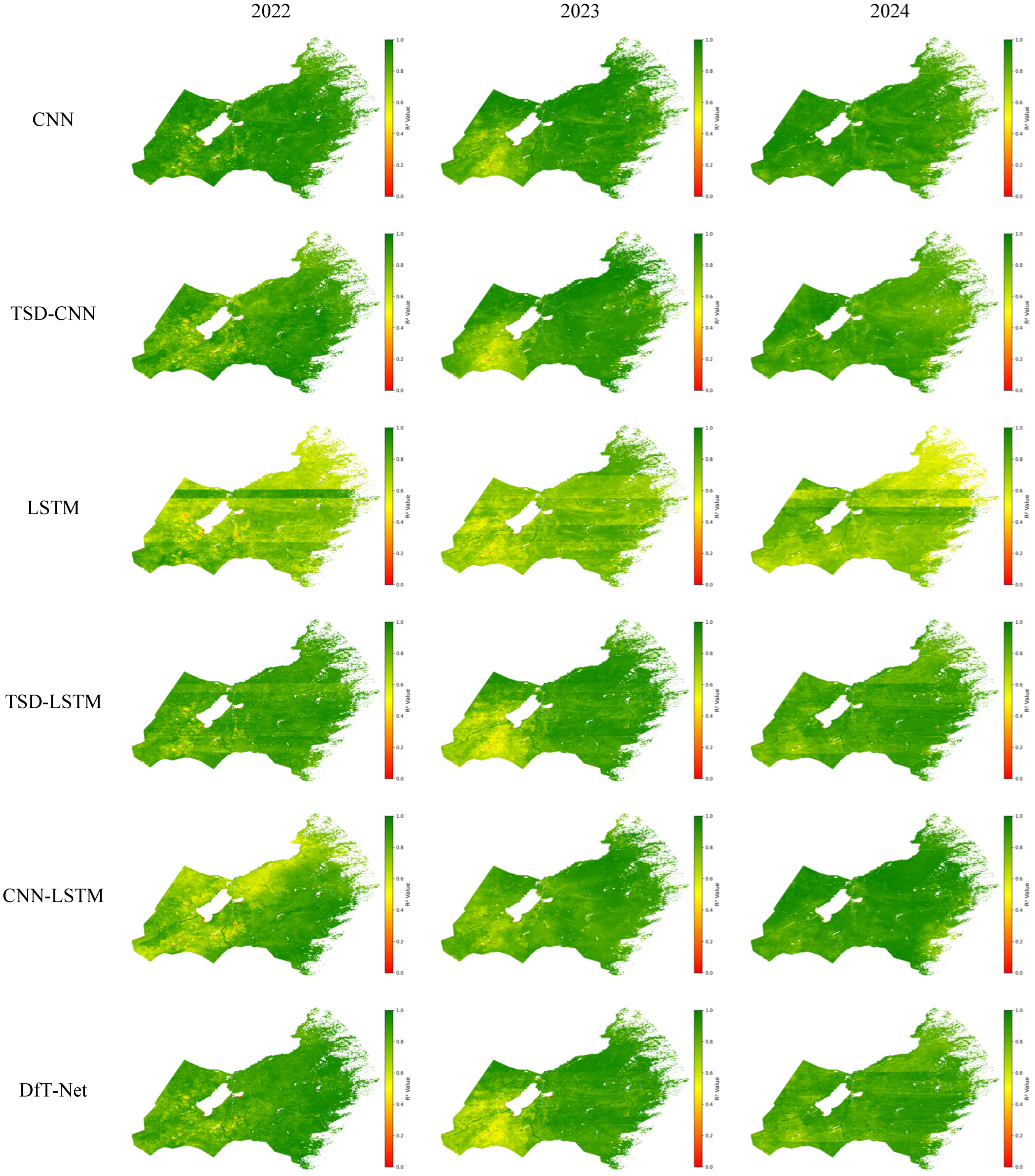
The annual R² values of all models were calculated pixel by pixel using monthly predictions from January to December, and the resulting pixel-level R² values were mapped according to their original geographic locations to generate the prediction-accuracy distribution maps shown in Figure 8. The results clearly indicate that CNN, TSD-CNN, and DfT-Net achieved high prediction accuracy at most individual locations, with the majority of pixels exhibiting R² values above 0.8 and only a few locations showing values between 0 and 0.2.

Figure 8. Spatial distribution of prediction accuracy (R²) for different models from January to December, 2022–2024.

In contrast, the LSTM model exhibited extensive yellow regions, indicating relatively low prediction accuracy. Among the three years evaluated, LSTM consistently showed the poorest performance, with R² values around 0.6. Except for the LSTM model, all other models exhibited an increasing trend in R² values from west to east, and the areas with the lowest prediction accuracy were mainly concentrated in the southwestern part of the Hulunbuir grassland.

The CNN-LSTM model showed lower accuracy in 2022 compared with the subsequent two years. In 2022, prediction accuracy in the western region was noticeably lower than that in the eastern region, whereas the model maintained relatively high accuracy across the entire study area in 2023 and 2024. This pattern was consistent with the overall evaluation results presented in Table 2.

Across the entire study area, no large-scale red or orange regions were observed, indicating that all six models were capable of providing effective pixel-level NDVI predictions.

Overall, the DfT-Net model achieved the highest prediction accuracy among all six models and demonstrated reliable pixel-level NDVI prediction performance across spatially distributed grassland pixels. Moreover, TSD preprocessing effectively provided additional temporal information, enabling the models to extract meaningful patterns from complex time series signals and improving overall NDVI prediction performance.

4. Discussion

4.1. Significance of Time Series Decomposition Preprocessing

Previous studies by Bandara et al. demonstrated that conventional LSTM models have limited capability in effectively capturing trend and seasonal patterns embedded in time series data [33]. Therefore, before LSTM training and prediction, decomposing non-stationary time series into two deterministic components (periodic and trend information) and one fluctuation component (random disturbances) can enable deep learning models to focus on relatively simple nonlinear relationships between individual features and NDVI, rather than requiring additional network capacity to identify complex nonlinear relationships hidden in mixed signals.

To ensure a reliable determination of the training duration, each model was trained repeatedly under the same experimental setting, and the epoch corresponding to the best validation performance was selected as the optimal training epoch. Based on these repeated training results, the CNN, LSTM, CNN-LSTM, TSD-CNN, TSD-LSTM, and DfT-Net models reached their respective best performance at approximately 55, 83, 50, 50, 65, and 40 epochs, respectively. The corresponding recorded training times were approximately 40, 59, 36, 34, 47, and 32 min.

The comparison shows that the TSD-based models generally reached their best validation performance with fewer or comparable training epochs than the corresponding models using the original meteorological sequences. For example, TSD-LSTM reached its best performance at approximately 68 epochs, compared with approximately 83 epochs for LSTM, while also achieving higher prediction accuracy. Although the TSD-based models contain multiple decomposed feature sequences and therefore involve a larger number of input features, the explicit representation of trend, seasonal, and residual characteristics may reduce the burden on the network to learn these temporal structures directly from mixed signals. This effect is particularly relevant to the present dataset because temperature and precipitation exhibit pronounced seasonal periodicity and recurrent interannual patterns. By separating these components, the models can process relatively more homogeneous temporal signals rather than simultaneously identifying long-term variation, seasonal repetition, and irregular fluctuations from the original sequences.

The shorter optimal training duration of TSD-LSTM therefore suggests that explicit temporal decomposition may facilitate the learning of recurrent and multi-scale temporal patterns. Although TSD introduces additional input features, it can reduce the difficulty of extracting temporal structures directly from the original mixed sequences.

These results suggest that TSD can improve the efficiency of temporal feature learning while enhancing prediction performance under the experimental settings of this study. However, the observed reduction in training epochs and training time should be interpreted as empirical results obtained under the specific experimental configuration rather than as evidence that TSD universally reduces computational complexity.

4.2. Influence of Deep Learning Model Combination

Previous studies by Bandara et al. demonstrated that conventional LSTM models have limited capability in effectively capturing trend and seasonal patterns embedded in time series data [33]. Therefore, before LSTM training and prediction, decomposing non-stationary time series into deterministic components representing trend and periodic information and a residual component representing irregular fluctuations can enable deep learning models to focus on relatively simple nonlinear relationships between individual features and NDVI, rather than requiring additional network capacity to identify complex nonlinear relationships hidden in mixed signals.

In this study, the comparison of prediction performance between models with and without TSD preprocessing demonstrated the effectiveness of TSD. Regardless of whether CNN, LSTM, or CNN-LSTM architectures were applied, models incorporating TSD preprocessing achieved higher prediction accuracy than their corresponding models without decomposition. These results indicate that decomposing meteorological time series into trend, seasonal, and residual components can provide more explicit temporal representations and facilitate the learning of meteorological–NDVI relationships.

The differences in prediction performance can be interpreted from the characteristics of the meteorological and NDVI time series and the feature extraction mechanisms of the models. The study data exhibited pronounced seasonal periodicity and recurrent interannual patterns. CNN can effectively extract local temporal patterns through convolution and parameter sharing, whereas LSTM is more suitable for modeling long-term temporal dependencies. The CNN-LSTM model therefore combines these complementary capabilities. Furthermore, TSD explicitly separates trend, seasonal, and residual components from the original meteorological sequences, reducing the difficulty of learning mixed temporal patterns. The superior performance of DfT-Net can therefore be attributed to the joint use of temperature and precipitation, their decomposed multi-scale temporal representations, and the complementary extraction of local and long-term temporal features.

To ensure a reliable comparison of model performance and computational efficiency, all models were trained under the same hardware and software environment, as summarized in Table 3. The experimental platform consisted of an Intel Core i9-12900H CPU, 32 GB RAM, and an NVIDIA GeForce RTX 3070 Ti Laptop GPU with 8 GB of VRAM. The models were implemented using TensorFlow 2.8.0. The operating system was Windows 11, and CUDA 12.0 was used to support GPU-based model training.

Table 3. Experimental environment and model training configuration.

Category	Configuration
CPU	Intel Core i9-12900H
GPU	NVIDIA GeForce RTX 3070 Ti Laptop GPU
RAM	32G
Deep Learning Framework	TensorFlow 2.8.0
CUDA	CUDA 12.0
System	Win 11

To determine the appropriate training duration, each model was repeatedly trained under the same experimental configuration, and the optimal epoch was determined according to the best validation performance obtained during training. The batch sizes, number of layers, optimal epochs, and recorded training times of the six models are summarized in Table 4. CNN, LSTM, CNN-LSTM, TSD-CNN, TSD-LSTM, and DfT-Net used batch sizes of 128, 64, 64, 128, 64, and 64, respectively, and contained 2, 2, 2, 6, 6, and 6 layers, respectively. The corresponding optimal epochs were 58, 83, 52, 53, 68, and 40, with recorded training times of approximately 40, 59, 36, 34, 47, and 32 min, respectively. The Adam optimizer was used for all models with an initial learning rate of 0.0001.

Table 4. Training epochs and recorded training time of different models.

Model	Batch Size	Layers	Optimal Epoch	Recorded Training Time (min)
CNN	128	2	58	40
LSTM	64	2	83	59
CNN-LSTM	64	2	52	36
TSD-CNN	128	6	53	34
TSD-LSTM	64	6	68	47
DfT-Net	64	6	40	32

The comparison shows that the TSD-based models generally achieved higher prediction accuracy while requiring fewer or comparable training epochs than their corresponding models using the original meteorological sequences. For example, TSD-LSTM reached its best performance at approximately 68 epochs, compared with approximately 83 epochs for LSTM, while also achieving higher prediction accuracy. Although the TSD-based models contained three times as many layers as their corresponding non-TSD models, their optimal training epochs and recorded training times did not increase proportionally. DfT-Net showed the shortest recorded training time among the evaluated models under the same computational environment. However, training time alone does not fully characterize computational complexity. Therefore, this result is considered only as an empirical observation of training efficiency rather than evidence of reduced computational cost. Overall, the results suggest that TSD can facilitate temporal feature learning and improve prediction performance under the experimental conditions of this study.

4.3. Effects of Temporal Scale

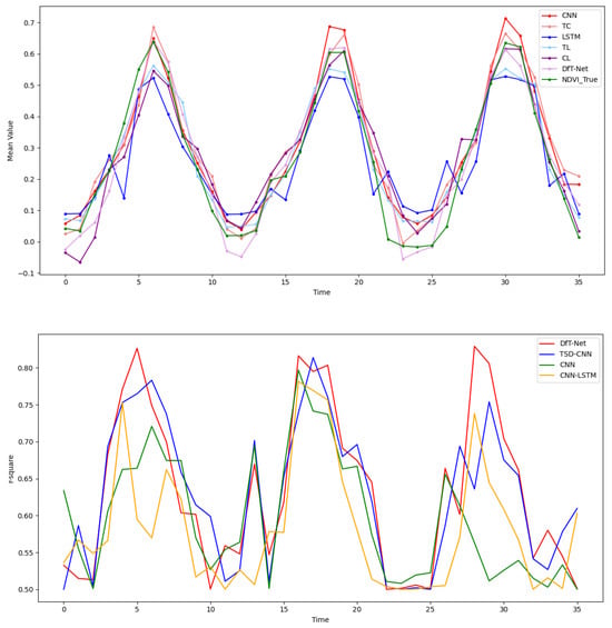
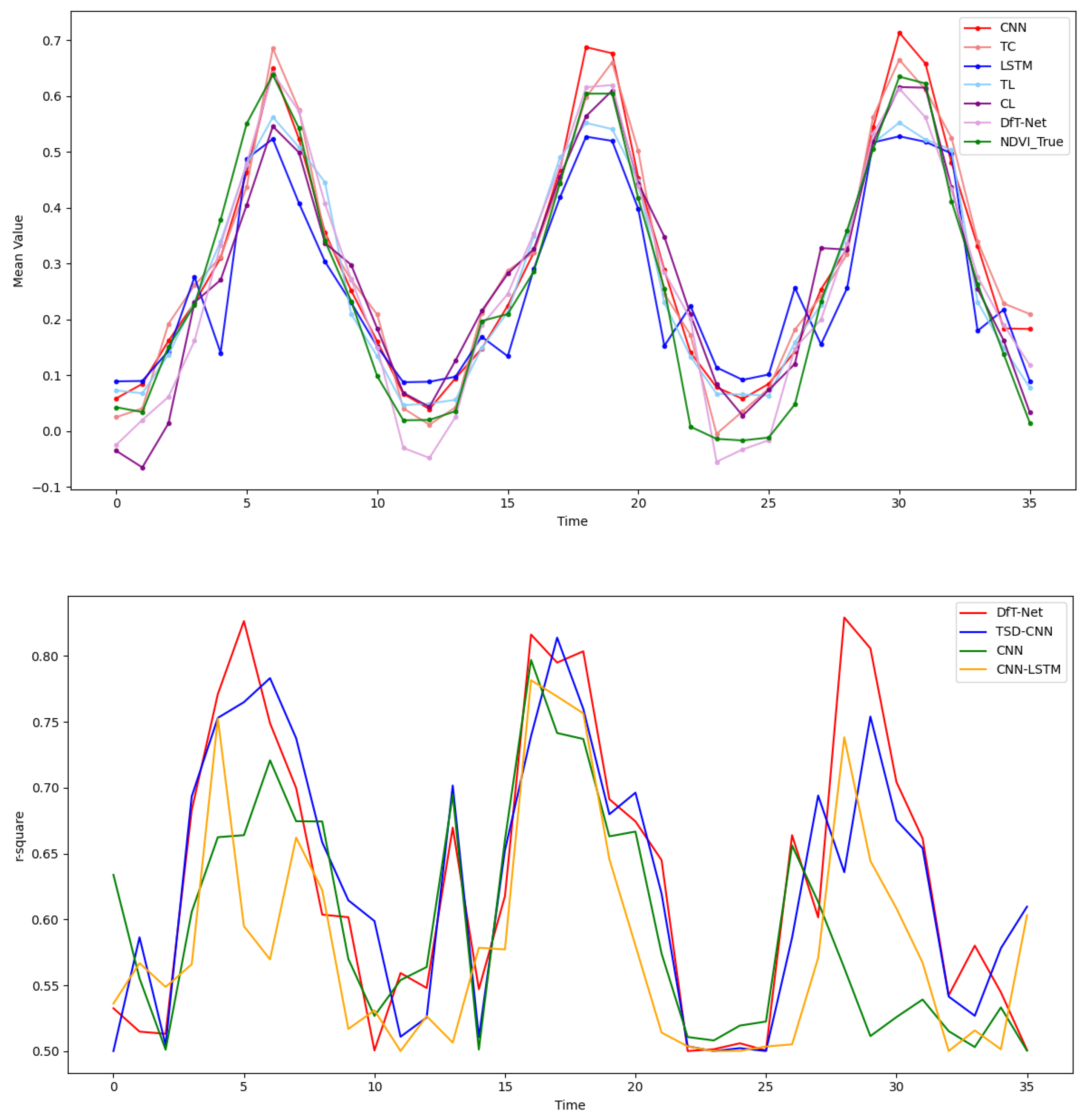
The monthly mean predicted NDVI values and corresponding R² values were calculated to investigate the influence of temporal scale, and the results are presented in Figure 9. At the monthly scale, all prediction results exhibited variation cycles consistent with the observed NDVI patterns.

Figure 9. Monthly variations in observed and predicted NDVI values and monthly prediction accuracy (R²) of different models.

Among the different models, the largest discrepancies occurred during the low-NDVI period from November to January and the peak-NDVI period from June to August. The LSTM and TSD-LSTM models showed relatively large deviations from the observed NDVI during these periods. Their predicted seasonal amplitudes were relatively small, resulting in underestimated NDVI values during peak vegetation growth periods and overestimated values during periods of low vegetation activity.

The CNN model showed a seasonal variation amplitude generally consistent with the observed NDVI, although its predicted values remained relatively higher than the observations. In contrast, DfT-Net, TSD-CNN, and CNN-LSTM maintained seasonal variation amplitudes that were closer to the observed NDVI throughout the year, indicating better consistency in capturing seasonal vegetation dynamics.

To further analyze the temporal variation in prediction accuracy, four high-performing models were selected, and pixel-level R² values were calculated for each month and presented as line graphs. The results showed that prediction accuracy exhibited a clear seasonal pattern that was broadly consistent with the seasonal dynamics of NDVI. Specifically, model accuracy was relatively lower during the non-growing season and generally increased during the vegetation growing season.

These results indicate that the predictive performance of the models varied with the seasonal state of vegetation. During the main growing season, temperature and precipitation provided relatively strong information for characterizing vegetation growth, allowing the meteorologically driven models to better capture NDVI variations. In contrast, prediction uncertainty tended to increase during the non-growing season and transitional periods. This seasonal variation suggests that factors beyond temperature and precipitation may also contribute to NDVI variability during specific periods. The potential influence of these factors and the resulting limitations of the dual-factor framework are discussed in Section 4.4.

4.4. Limitations and Future Directions

Despite the satisfactory prediction performance of DfT-Net, several limitations should be acknowledged. The proposed model primarily uses temperature and precipitation as the two meteorological driving factors and therefore does not explicitly represent other environmental and anthropogenic factors that may affect grassland vegetation dynamics.

In particular, grazing and harvesting activities may cause rapid changes in vegetation conditions during specific periods of the year. For example, the relatively rapid decline in NDVI observed around September may be partly associated with grass harvesting and grazing activities in the Hulunbuir grassland. Such anthropogenic disturbances cannot be fully characterized by temperature and precipitation alone and may therefore contribute to prediction uncertainty during this period.

Snow-related processes represent another potential source of uncertainty, particularly during the non-growing season. During winter, precipitation in the form of snow does not immediately contribute to vegetation or soil water availability. Snow cover may also affect the remote-sensing observation of vegetation and consequently influence the observed NDVI. Moreover, the ecological effects of winter precipitation may be delayed until snowmelt in the following spring, resulting in a temporal lag between meteorological forcing and vegetation response. These processes are not explicitly represented in the current dual-factor framework.

Therefore, DfT-Net should be regarded as a dual-factor meteorological-driven prediction framework rather than a comprehensive model incorporating all ecological controls. The current design intentionally focuses on temperature and precipitation because of their important roles in grassland vegetation dynamics and their potential compatibility with future meteorological forecasting applications. Nevertheless, incorporating additional forecastable environmental and anthropogenic variables may further improve the representation of complex vegetation responses.

Future studies could extend the DfT-Net framework by incorporating snow-cover information, soil moisture, grazing intensity, grassland management information, and other relevant ecological variables. Such extensions may improve the model’s ability to characterize non-meteorological influences and further enhance spatially distributed pixel-level NDVI forecasting.

5. Conclusions

This study developed a dual-factor-driven temporal network (DfT-Net) for spatially distributed pixel-level monthly NDVI forecasting in the Hulunbuir grassland, Inner Mongolia, China. Using MODIS NDVI and ERA5-Land temperature and precipitation data from 2013 to 2024, the proposed framework was evaluated against several deep learning models under the same experimental setting.

The temporal analysis showed that temperature, precipitation, and NDVI exhibited clear seasonal periodicity and recurring annual variation patterns. These periodic characteristics reflect the temporal response of grassland vegetation to seasonal climatic conditions. The X-12-ARIMA method was used to decompose the temperature and precipitation sequences into trend, seasonal, and residual components, thereby separating temporal information at different scales and providing decomposed meteorological representations for subsequent model training. The decomposition of NDVI was used only for preliminary temporal analysis and was not used as a model input or training feature.

DfT-Net achieved an RMSE of 0.100, an MAE of 0.074, and an R² of 0.828, showing the best overall performance among the comparative models, including LSTM, CNN, TSD-CNN, TSD-LSTM, and CNN-LSTM, under the experimental conditions of this study. The results suggest that combining dual-factor meteorological information with time series decomposition can improve the representation of meteorological–vegetation relationships and contribute to improved NDVI prediction performance.

From the perspective of temporal feature modeling, the proposed framework incorporates periodic and multi-scale temporal information into the prediction process. The TSD procedure separates the seasonal structure and other temporal components of meteorological drivers, while the CNN extracts local temporal patterns through shared convolutional parameters. The LSTM subsequently models longer-term temporal dependencies across the input sequence. This combination enables DfT-Net to represent recurring temporal patterns in grassland vegetation dynamics and provides a temporal modeling framework for spatially distributed pixel-level NDVI prediction.

For spatially distributed prediction, DfT-Net was applied independently to valid 1000 m grassland pixels, with the same model parameters shared across pixels. The model does not explicitly model spatial dependencies or interactions between neighboring pixels. Instead, each pixel provides an independent temporal prediction sequence, and the resulting predictions are assigned back to their original geographic locations to generate spatially distributed NDVI prediction maps. The regional mean time series presented in the preliminary analysis were used only to characterize the overall temporal variation in the study area and were not used for model training or prediction.

Nevertheless, several limitations should be acknowledged. The current framework focuses on temperature and precipitation as the primary driving factors and does not explicitly incorporate other potentially important environmental and anthropogenic influences, such as soil moisture, grazing, harvesting, snow cover, and delayed snowmelt. These factors may contribute to prediction uncertainty during specific periods, particularly during the non-growing season and transitional periods. In addition, the current evaluation was conducted within the study period and experimental conditions considered in this work. Therefore, the reported results demonstrate the potential of DfT-Net under the present experimental setting rather than universal or operational forecasting capability.

Overall, DfT-Net provides a potential framework for integrating decomposed meteorological drivers and multi-scale temporal features into spatially distributed pixel-level grassland NDVI forecasting. The framework may provide a useful reference for regional grassland vegetation monitoring based on pixel-level predictions. Future studies should incorporate additional forecastable environmental and anthropogenic factors and conduct evaluations across different regions and forecasting scenarios to further assess the generalizability and practical applicability of the proposed approach.

References

- Huang, S.Z.; Ming, B.; Huang, Q.; Leng, G.; Hou, B. A Case Study on a Combination NDVI Forecasting Model Based on the Entropy Weight Method. Water Resour. Manag. 2017, 31, 3667–3681. [Google Scholar] [CrossRef] [Scilit]
- Liu, X.; Zhu, X.; Pan, Y.; Li, Y.; Zhao, A. Spatiotemporal Changes in Vegetation Coverage in China during 1982–2012. Acta Ecol. Sin. 2015, 35, 5331–5342. [Google Scholar] [CrossRef] [Scilit]
- Cao, Y.G.; Liu, C. The Development of Snow-Cover Mapping from AVHRR to MODIS. Geogr. Geo-Inf. Sci. 2005, 5, 15–19. [Google Scholar]
- Li, C.E.; Ma, J.; He, Z. Change Characteristic Analysis of Natural Vegetation Coverage in Yili River Valley. Geospat. Inf. 2022, 20, 84–88. [Google Scholar]
- Wang, Y.N.; Kong, X.B.; Zhao, C.J.; Yao, G.Q.; Guo, K. Change of Vegetation Coverage in the Loess Plateau from 2000 to 2020 and Its Spatiotemporal Pattern Analysis. J. Soil Water Conserv. 2022, 36, 130–137. [Google Scholar]
- Qu, X.B.; Wang, Y.P.; Gao, S.X.; Zhang, X.M.; Xin, X.F.; Ao, M.Q. Temporal and Spatial Change of NDVI and Its Response to Climatic Conditions in Hulun Buir Region from 2000 to 2020. J. Meteorol. Environ. 2022, 38, 57–63. [Google Scholar]
- Bianchi, E.; Villalba, R.; Solarte, A. NDVI Spatio-Temporal Patterns and Climatic Controls over Northern Patagonia. Ecosystems 2019, 23, 84–97. [Google Scholar] [CrossRef] [Scilit]
- Wu, T.S.; Fu, H.P.; Feng, F.; Bai, H.M. A New Approach to Predict Normalized Difference Vegetation Index Using Time-Delay Neural Network in the Arid and Semi-Arid Grassland. Int. J. Remote Sens. 2019, 40, 9050–9063. [Google Scholar] [CrossRef] [Scilit]
- Li, Y.H.; Jiang, T.; Guo, Q.H. Temporal Spatial Variation and Prediction Analysis of Vegetation Coverage in the Loess Plateau. Beijing Surv. Mapp. 2020, 34, 1564–1569. [Google Scholar]
- Jia, S.T.; Huang, S.Z.; Wang, H.; Li, Z.Y.; Huang, Q.; Liang, H. Simulation of Vegetation Change Based on BP-SVM Model. Arid. Zone Res. 2021, 38, 1085–1093. [Google Scholar]
- Pérez-Alarcón, A.; Garcia-Cortes, D.; Fernández-Alvarez, J.C.; Martínez-González, Y. Improving Monthly Rainfall Forecast in a Watershed by Combining Neural Networks and Autoregressive Models. Environ. Process. 2022, 9, 53. [Google Scholar] [CrossRef] [Scilit]
- Pan, X.L.; Zhang, Z.; Jiang, T.; Sui, B.K.; Sun, Y.C. An Approach of the Convolutional Long Short-Term Memory Network for NDVI Prediction. Geomat. World 2020, 27, 60–67. [Google Scholar]
- Reddy, D.S.; Prasad, P.R.C. Prediction of Vegetation Dynamics Using NDVI Time Series Data and LSTM. Model. Earth Syst. Environ. 2018, 4, 409–419. [Google Scholar] [CrossRef] [Scilit]
- Zhao, F.; Yang, G.; Yang, H.; Zhu, Y.; Meng, Y.; Han, S.; Bu, X. Short and Medium-Term Prediction of Winter Wheat NDVI Based on the DTW–LSTM Combination Method and MODIS Time Series Data. Remote Sens. 2021, 13, 4660. [Google Scholar] [CrossRef] [Scilit]
- Guo, Y.; Zhang, L.; He, Y.; Cao, S.; Li, H.; Ran, L.; Ding, Y.; Filonchyk, M. LSTM Time Series NDVI Prediction Method Incorporating Climate Elements: A Case Study of Yellow River Basin, China. J. Hydrol. 2024, 629, 130518. [Google Scholar] [CrossRef] [Scilit]
- Zhao, F.; Xu, N.; Fang, Z.; Bai, S.; Jiang, M.; Zhu, Y. A New Approach for Predicting NDVI of Winter Wheat Using Seasonal LSTM. J. Indian Soc. Remote Sens. 2025, 3, 2419–2434. [Google Scholar] [CrossRef] [Scilit]
- Liu, S.; Ji, H.; Wang, M.C. Nonpooling Convolutional Neural Network Forecasting for Seasonal Time Series with Trends. IEEE Trans. Neural Netw. Learn. Syst. 2020, 31, 2879–2888. [Google Scholar] [CrossRef] [Scilit] [PubMed]
- Zarei, A.R.; Mahmoudi, M.R. Investigating the Ability of Periodically Correlated (PC) Time Series Models to Forecast the Climate Index. Stoch. Environ. Res. Risk Assess. 2020, 34, 121–137. [Google Scholar] [CrossRef] [Scilit]
- Gao, P.; Du, W.; Lei, Q.; Li, J.; Zhang, S.; Li, N. NDVI Forecasting Model Based on the Combination of Time Series Decomposition and CNN–LSTM. Water Resour. Manag. 2023, 37, 1481–1497. [Google Scholar] [CrossRef] [Scilit]
- Farbo, A.; Sarvia, F.; De Petris, S.; Basile, V.; Borgogno-Mondino, E. Forecasting Corn NDVI through AI-Based Approaches Using Sentinel-2 Image Time Series. ISPRS J. Photogramm. Remote Sens. 2024, 211, 244–261. [Google Scholar] [CrossRef] [Scilit]
- Su, Z.; Shen, J.; Sun, Y.; Hu, R.; Zhou, Q.; Yong, B. Deep Spatio-Temporal Fuzzy Model for NDVI Forecasting. IEEE Trans. Fuzzy Syst. 2024, 33, 290–301. [Google Scholar] [CrossRef] [Scilit]
- Iele, I.; Romoli, G.; Molino, D.; Ayllón, E.M.; Ruffini, F.; Soda, P.; Tortora, M. Probabilistic NDVI Forecasting from Sparse Satellite Time Series and Weather Covariates. arXiv 2026, arXiv:2602.17683. [Google Scholar]
- Hou, L. Impact of COVID-19 on Latent Emissiveness of Residents in China: Based on the X-12-ARIMA Additive Seasonal Adjustment Model. J. Comput. Methods Sci. Eng. 2021, 21, 1591–1604. [Google Scholar] [CrossRef] [Scilit]
- Guo, H.Y.; Chen, Q.X.; Xia, Q.; Kang, C.Q.; Zhang, X. A Monthly Electricity Consumption Forecasting Method Based on Vector Error Correction Model and Self-Adaptive Screening Method. Int. J. Electr. Power Energy Syst. 2018, 95, 427–439. [Google Scholar] [CrossRef] [Scilit]
- Su, T.; Feng, T.C.; Huang, B.H.; Han, Z.X.; Qian, Z.H.; Feng, G.L.; Hou, W. Trend, Seasonal, and Irregular Variations in Regional Actual Evapotranspiration over China: A Multi-Dataset Analysis. Front. Phys. 2021, 9, 718771. [Google Scholar] [CrossRef] [Scilit]
- Findley, D.F.; Monsell, B.C.; Bell, W.R.; Otto, M.C.; Chen, B.C. New Capabilities and Methods of the X-12-ARIMA Seasonal-Adjustment Program. J. Bus. Econ. Stat. 1998, 16, 127–152. [Google Scholar] [CrossRef] [Scilit]
- Shin, S.; Her, Y.; Muñoz-Carpena, R.; Khare, Y.P. Multi-Parameter Approaches for Improved Ensemble Prediction Accuracy in Hydrology and Water Quality Modeling. J. Hydrol. 2023, 622, 129458. [Google Scholar] [CrossRef] [Scilit]
- Yan, B.; Mu, R.; Guo, J.; Liu, Y.; Tang, J.; Wang, H. Flood Risk Analysis of Reservoirs Based on Full-Series ARIMA Model under Climate Change. J. Hydrol. 2022, 610, 127979. [Google Scholar] [CrossRef] [Scilit]
- Li, Y.; Wang, W.; Wang, G.; Tan, Q. Actual Evapotranspiration Estimation over the Tuojiang River Basin Based on a Hybrid CNN-RF Model. J. Hydrol. 2022, 610, 127788. [Google Scholar] [CrossRef] [Scilit]
- He, Y.; Yao, S.; Chen, Y.; Yan, H.; Zhang, L. Spatiotemporal Prediction of Time-Series InSAR Land Subsidence Based on ConvLSTM Neural Network. Geomat. Inf. Sci. Wuhan Univ. 2025, 50, 483–496. [Google Scholar]
- Zhao, Z.; He, Y.; Yao, S.; Wang, Y.; Wang, W.; Zhang, L.; Sun, Q. A Comparative Study of Different Neural Network Models for Landslide Susceptibility Mapping. Adv. Space Res. 2022, 70, 383–401. [Google Scholar] [CrossRef] [Scilit]
- Wang, W.C.; Cheng, Q.; Chau, K.W.; Hu, H.; Zang, H.F.; Xu, D.M. An Enhanced Monthly Runoff Time Series Prediction Using Extreme Learning Machine Optimized by Salp Swarm Algorithm Based on Time Varying Filtering Based Empirical Mode Decomposition. J. Hydrol. 2023, 620, 129460. [Google Scholar] [CrossRef] [Scilit]
- Bandara, K.; Bergmeir, C.; Smyl, S. Forecasting across Time Series Databases Using Recurrent Neural Networks on Groups of Similar Series: A Clustering Approach. Expert Syst. Appl. 2020, 140, 112896. [Google Scholar] [CrossRef] [Scilit]
Disclaimer/Publisher’s Note: The statements, opinions and data contained in all publications are solely those of the individual author(s) and contributor(s) and not of MDPI and/or the editor(s). MDPI and/or the editor(s) disclaim responsibility for any injury to people or property resulting from any ideas, methods, instructions or products referred to in the content. |
© 2026 by the authors. Licensee MDPI, Basel, Switzerland. This article is an open access article distributed under the terms and conditions of the Creative Commons Attribution (CC BY) license.