


Abstract
Urban pollutant dispersion is governed by highly nonlinear interactions between flow structures, turbulence characteristics, and scalar transport processes, making accurate prediction computationally demanding. The present study investigates pollutant dispersion behaviour within an idealised urban configuration using a combined computational fluid dynamics (CFD) and surrogate machine learning. Reynolds-averaged Navier–Stokes simulations were performed to analyse the effects of Reynolds number, Schmidt number, turbulence kinetic energy, concentration transport, velocity distribution, and injection ratio on flow symmetry and pollutant redistribution. The numerical results showed that variations in Reynolds number and injection ratio modified the spatial organisation and relative symmetry of the computed vorticity and concentration fields, together with the corresponding centreline concentration, velocity, and turbulent kinetic energy responses. To complement the CFD analysis, an Extreme Gradient Boosting (XGBoost) model was trained to predict concentration, velocity, and turbulence kinetic energy using CFD-generated datasets. Feature importance analysis further revealed physically meaningful relationships among the governing transport variables, with Reynolds number dominating velocity and turbulence kinetic energy behaviour, while concentration transport remained strongly influenced by injection ratio.
1. Introduction
Air pollution in urban environments has become a critical global concern due to its direct impact on human health, environmental sustainability, and urban liveability. The dispersion of pollutants in cities is governed by complex interactions between atmospheric flow, built structures, and emission sources. In densely built environments, such as street canyons and building clusters, airflow is significantly altered by obstacles, leading to highly heterogeneous and localised concentration fields. These flow modifications can result in pollutant accumulation zones, reduced ventilation efficiency, and increased exposure risks [1,2,3]. Therefore, understanding the mechanisms governing airflow and pollutant transport in urban configurations is essential for effective urban planning and environmental management.
From a fluid mechanics perspective, symmetry plays a fundamental role in determining flow behaviour and transport processes [4,5,6,7]. In idealised configurations, geometric symmetry in the domain and boundary conditions often leads to symmetric flow structures, which can simplify both analysis and prediction [8,9,10]. Many urban layouts, particularly regular building arrays and simplified street canyon models, exhibit nominal geometric symmetry. Under such conditions, velocity fields, vorticity distribution, and scalar transport patterns are expected to follow symmetric configurations [4,11]. However, the presence of nonlinear interactions in fluid flow means that such symmetry is often only preserved under limited conditions. In practical scenarios, fluid flows frequently undergo symmetry breaking due to the dominance of inertial forces, turbulence generation, and complex interactions between flow structures and obstacles. As the Reynolds number increases, the flow transitions from a relatively ordered and symmetric state to a more chaotic regime characterised by vortex shedding, recirculation zones, and wake interactions. These processes disrupt the initial symmetry of the system, leading to asymmetric velocity fields and nonuniform pollutant dispersion patterns. In urban environments, such symmetry breaking is particularly significant, as it directly influences pollutant accumulation, mixing efficiency, and exposure distribution within built-up areas.
Computational fluid dynamics (CFD) has been widely employed to investigate airflow and pollutant dispersion in urban environments, offering detailed insights into flow structures and scalar transport phenomena. Approaches such as Reynolds-averaged Navier–Stokes (RANS) [12,13,14] and large eddy simulation (LES) [11,15,16] have been extensively used to simulate urban flows with varying degrees of accuracy and computational demand. While these methods are effective in capturing general flow behaviour, they often face limitations when dealing with highly complex, unsteady, and turbulent flow regimes typical of urban settings. In particular, many studies have focused primarily on descriptive analysis of flow patterns and concentration fields, without explicitly examining the role of symmetry in governing dispersion processes. Furthermore, high-fidelity simulations can be computationally expensive, limiting their applicability for rapid assessment or real-time decision making.
In recent years, machine learning (ML) has emerged as a powerful tool for augmenting traditional CFD approaches by providing fast and efficient surrogate models for complex fluid systems [17,18,19]. ML models are capable of learning nonlinear relationships between input parameters and flow responses, enabling rapid prediction of key quantities such as velocity, concentration, and energy distribution. This capability is particularly valuable in scenarios where repeated simulations are required across a wide parameter space. However, despite their predictive strength, many ML models operate as black-box systems, offering limited physical interpretability and weak connections to the underlying transport mechanisms governing the flow. Recent studies have demonstrated that ensemble learning approaches, particularly tree-based algorithms such as Extreme Gradient Boosting (XGBoost), can effectively capture complex multivariate interactions associated with pollutant transport and turbulent flow behaviour [20]. In addition to strong predictive capability, such models provide feature-importance analysis that enables the identification of dominant governing parameters influencing transport behaviour. When integrated with CFD-generated datasets, machine learning frameworks, therefore, offer the potential to bridge data-driven modelling with physically interpretable fluid dynamics analysis. In the context of urban pollutant dispersion, ML-assisted surrogate modelling can be particularly useful for rapidly exploring the influence of Reynolds number, turbulence characteristics, and scalar transport behaviour on symmetry preservation, symmetry breaking, and pollutant redistribution patterns within complex urban flow environments.
A substantial body of research has been dedicated to understanding airflow behaviour and pollutant dispersion in urban environments using both numerical and data-driven approaches. These studies have progressively advanced the understanding of flow structures, dispersion mechanisms, and the influence of geometric and environmental factors. At the same time, recent developments in machine learning have introduced new opportunities for efficient prediction and analysis.
Hassan et al. [11] conducted a detailed investigation of pollutant dispersion within urban street canyons using an LES approach. Their study highlighted the significant influence of building symmetry and asymmetry on flow structure and pollutant concentration distribution. The key findings of this study indicate that the three-dimensional interaction between dominant canyon vortices and the roof-level flow plays a crucial role in determining pollutant concentration levels along the windward walls. In particular, the extent of corner eddies and their interaction with the primary vortical structures were found to significantly influence ventilation efficiency within the canyon. These findings also highlight the potential for further refinement of such analyses, particularly in accounting for additional urban features such as vegetation within street canyons. Further investigation on their influence on flow and dispersion characteristics, supported by appropriate modelling strategies, would contribute to a more comprehensive understanding of urban pollutant transport.
Building on this, Ali et al. [12] examined the role of urban morphology, including variations in building arrangement and canyon geometry, on airflow and pollutant transport by a hybrid finite volume method (FVM)–RANS approach. Their findings revealed that geometric modifications can significantly alter recirculation zones, ventilation efficiency, and pollutant accumulation behaviour. Nevertheless, the analysis was largely centred on geometric effects and their influence on flow structures, with limited emphasis on the underlying flow organisation. In particular, the evolution of flow structures from more ordered to complex states under changing flow conditions was not explicitly characterised, suggesting an opportunity for further investigation into the fundamental behaviour governing these transitions.
In addition to steady-state analyses, Du et al. [3] investigated the influence of time-dependent inflows on pollutant dispersion within an idealised two-dimensional street canyon using LES. Their study demonstrated that unsteady inflow conditions significantly enhance pollutant removal efficiency compared to steady inflow cases, particularly at higher amplitudes and shorter periods. This enhancement was attributed to intensified turbulent transport mechanisms, including dominant counter-gradient mass flux and increased frequency of ejection and sweep events, which promote the exchange of polluted and fresh air within the canyon. While this work offered important insight into the temporal variability of urban flow behaviour, the analysis was conducted within an idealised two-dimensional configuration under isothermal conditions. As such, the interaction between unsteady inflow conditions, three-dimensional flow organisation, and structural characteristics of the flow field remains an area for further exploration, particularly in the context of more complex and realistic urban environments.
Che and Zhuang [21] extended the analysis of urban pollutant dispersion by incorporating coupled thermo-fluid and environmental effects through the inclusion of vegetation within street canyons. Using a validated three-dimensional CFD framework, the study examined the combined influence of street trees and vertical greening on airflow, temperature distribution, and pollutant transport. The results demonstrated that integrated vegetation systems can simultaneously reduce near-building temperatures and significantly enhance pollutant removal efficiency, achieving removal rates of up to when vertical greening is combined with street trees. These effects were attributed to modifications in airflow structure, including reduced wind speeds and more uniform distribution of flow and scalar fields within the canyon. The analysis was conducted within a simplified and idealised configuration, where vegetation was represented in an approximate manner and broader urban-scale influences such as symmetry and asymmetry of street canyons, wind direction were not explicitly considered. As such, while the study effectively highlighted the impact of added physical complexity, the systematic interpretation of how these interacting factors influence the organisation of flow structures and dispersion behaviour remains an area for further investigation. In parallel with advances in CFD-based modelling, data-driven approaches have been increasingly adopted to predict and analyse pollutant dispersion in urban environments. Some recent works [17,18,22] demonstrated that machine learning techniques can effectively capture complex, nonlinear relationships between governing parameters and pollutant concentration levels, offering a computationally efficient alternative to high-fidelity simulations. These approaches have shown strong predictive capability across a range of environmental conditions and configurations. However, the primary focus of such models is often on prediction accuracy, with comparatively less emphasis on linking the learned relationships to the underlying physical processes. Although recent developments in ML have begun to address this limitation, the integration of data-driven methods with physically interpretable flow structures remains an emerging area of research.
Despite significant advances in CFD-based urban flow modelling and the growing use of machine learning techniques, limited attention has been given to the systematic interpretation of spatial symmetry characteristics in pollutant-dispersion fields under varying governing parameters. Existing studies commonly focus either on detailed numerical simulations or on predictive modelling, with comparatively less emphasis on relating parameter-dependent changes in flow organisation and scalar distribution to interpretable surrogate predictions. A controlled framework that combines parametric CFD analysis with surrogate modelling can therefore provide useful insight into the relationships among flow conditions, pollutant transport, and the spatial organisation of the resulting fields.
The present study investigates airflow and pollutant dispersion in an idealised geometrically symmetric urban building array, with particular emphasis on the evolution of spatial symmetry characteristics in the computed flow and scalar fields as the governing parameters vary. The flow is modelled using a Reynolds-averaged Navier–Stokes framework with the standard k– turbulence model, and the effects of Reynolds number, Schmidt number, and injection ratio are systematically examined. The numerical analysis evaluates the corresponding variations in vorticity, concentration distribution, centreline velocity, and turbulent kinetic energy. In addition, an XGBoost-based surrogate framework is developed to predict selected CFD-derived scalar responses and assess the relative influence of the governing parameters. The surrogate models are intended to complement the CFD analysis by enabling rapid prediction within the investigated parameter space.
2. Mathematical Formulation
2.1. Physical Model Description
In the present investigation, geometric symmetry is employed as a controlled reference for examining parameter-dependent changes in flow and scalar-field organisation, consistent with the broader role of symmetry in simplifying and interpreting thermal-fluid systems [23]. Figure 1 represents the schematic diagram of this investigation. The rectangular domain is 30 D in streamwise length and 10 D in crosswise length, where D = 1. The left wall is the inlet, the right wall is the outlet, and the top and bottom walls are symmetric. The cylindrical-shaped pollutant source was split into four equal pieces. Pollutant gas inlets are two arcs that are diametrically opposed to one another (Figure 1 shows these arcs as limits with dotted lines). These arcs inject pollutant gas with a constant velocity, . The solid lines on the remaining cylinder surfaces are subject to a no-slip wall condition. With a steady free-stream velocity , air enters from the left wall of the channel.
Figure 1.
The schematic diagram of the square domain with building and pollution source.
The computational configuration was deliberately selected as an idealised geometrically symmetric reference arrangement rather than as a representation of a particular urban site or an established experimental benchmark. The repeated building array and the diametrically opposed pollutant-injection arcs provide a controlled spatial configuration about the domain centreline. This arrangement allows the individual effects of Reynolds number, Schmidt number, and injection ratio to be examined while keeping the geometry and source position unchanged. Consequently, parameter-dependent changes in the spatial organisation and relative symmetry of the vorticity, concentration, velocity, and turbulent kinetic energy fields can be interpreted with respect to a common reference configuration.
Symmetry is widely employed in thermal-fluid and computational fluid dynamics studies to simplify geometric descriptions, isolate governing physical mechanisms, and improve the efficiency and interpretation of numerical analyses [23]. Caetano [23] also emphasised that the suitability of a symmetry assumption must be evaluated for the specific physical problem because an imposed symmetry may obscure important asymmetric or unstable behaviour under some conditions. In the present study, geometric symmetry is used as a controlled reference for comparing the computed field characteristics rather than as evidence that all resulting flow and dispersion fields must remain perfectly symmetric. The adopted configuration is therefore intended to support a systematic parametric investigation and is not presented as a universal urban geometry or an internationally standardised validation case [24,25].
2.2. Governing Equations for Turbulence and Scalar Transport
In this study, the flow is two-dimensional, turbulent, unsteady, and incompressible. The following governing Navier–Stokes equations are used for flow [26]:
where
- is the velocity vector;
- p is the pressure;
- is the density;
- is the kinematic viscosity;
- is the turbulent viscosity.
Standard k- Model
The typical k- turbulence model, first introduced by Launder and Spalding [27], is among the most used two-equation models for modelling turbulent flows. This model addresses transport equations for turbulent kinetic energy (k) and its dissipation rate (), using a linear eddy viscosity hypothesis to correlate Reynolds stresses with mean velocity gradients. The model relies on the premise of isotropic turbulence and employs experimentally derived constants to guarantee accurate predictions throughout a wide spectrum of canonical flows. The typical k- model is recognized for its simplicity, resilience, and comparatively cheap computing expense; yet, it has certain limitations. It may have difficulty precisely capturing the impacts of pronounced streamline curvature, rotation, and flows characterized by substantial separation or intricate recirculation zones. Nonetheless, the traditional k- model continues to be favoured for its adequate accuracy in free shear flows, including jets and mixing layers, as well as its established dependability in engineering applications related to wall-bounded turbulent flows [27,28].
The turbulence closure is provided by the standard k- model [29,30]:
- k is the turbulent kinetic energy.
- is the turbulence dissipation rate.
- is the production term of turbulent kinetic energy.
- is the Prandtl number for turbulent kinetic energy.
- is the Prandtl number for the dissipation rate.
- and are model constants in the turbulence dissipation rate equation.
- represents the rate of energy transfer from turbulence to dissipation, and represents the rate of energy loss due to dissipation.
The advection–diffusion equation is used to represent the transport of a conserved scalar quantity [26]:
where
- C is the scalar concentration field;
- is the diffusion coefficient.
We define the dimensionless ratio of the velocity of fluid injection to the free stream velocity. Here, is for the no-injection case and increased with increasing injection velocity.
The governing equations are solved in nondimensional form. The characteristic length scale is the side length of the square buildings, D, and the characteristic velocity scale is the uniform free-stream (inlet) velocity . All lengths are therefore normalised by D and all velocities by and the source concentration as the scalar scale, so that the prescribed inlet condition becomes . The two dimensionless groups governing the present problem are the Reynolds number and the Schmidt number, defined as
where is the free-stream velocity, D is the side length of the square buildings, is the kinematic viscosity of the fluid, and is the molecular diffusivity of the transported scalar introduced in Equation (6). In the normalised formulation adopted here, the density is unity and the inlet velocity is , so that the kinematic viscosity and the scalar diffusivity are prescribed directly as and . The Reynolds and Schmidt numbers therefore enter the governing equations as the sole control parameters, and all reported field variables are dimensionless.
The turbulent viscosity and the turbulent kinetic energy production term is defined as [31]
The constants , , , , and are empirically calibrated to ensure accurate performance of the k- turbulence model for a wide range of canonical turbulent flows. The standard model constants used in this study are
The particle tracing is performed by solving the following equations:
where
- is the position vector of the particle at time t.
- m is the particle mass.
- is the particle velocity.
- is the drag force acting on the particle.
- is the kinematic viscosity of the fluid.
- is the particle diameter.
- t is the time of release for the particles.
In this study, the tracked particles are considered to be spherical, rigid, and sufficiently sparse, allowing us to apply a one-way coupling between the particles and the fluid. The specific values for particle diameter, density, and mass will be inserted here. As the particle Reynolds number stays well below one across the computational domain, the motion of the particles is mainly influenced by viscous drag. As a result, the Stokes drag model is used to characterize the drag force acting on the particles. Other hydrodynamic forces like lift, virtual mass, Basset history force, Brownian motion, and interactions between particles have been overlooked, as their effects are minimal given the current flow conditions. In the COMSOL particle tracing module, the particle properties with a diameter of and a density of = 1 kg/m3 were set. To model the drag force, the built-in Stokes drag formulation was used, as the particle Reynolds number stayed within the Stokes flow regime during the entire simulation process.
2.3. Boundary Conditions
The computational domain is bounded by four boundaries: the left and right boundaries, which act as the inlet and the outlet, respectively, and the upper and lower boundaries, which are aligned with the streamwise direction and carry neither inflow nor outflow. The boundary conditions for the airflow and pollutant dispersion model of the rectangular domain are as follows:
Left boundary (Inlet):
Right boundary (Outlet):
Bottom boundary (Symmetry):
Top boundary (Symmetry):
The boundary conditions for the airflow and pollutant dispersion model of the cylinder are as follows (considering the cylinder has four arcs):
Bottom Arc (Inlet-1):
Top Arc (Inlet-2):
The buildings and the left and right arcs of the cylinder are treated as no-slip walls (); a zero normal scalar flux is imposed on the building surfaces and on the lateral arcs of the source. The scalar concentrations are expressed in normalised form, with denoting the background (clean-air) value and the source value, and the pressure is normalised by .
3. Grid Independence Test and Code Validation
3.1. Grid Independent Test
A grid independence test was carried out using three successively refined meshes containing 136,364, 174,932 and 429,898 elements, at a fixed injection ratio = 0.3. The wake-averaged normalised concentration was monitored at , downstream of the building array, for the three Reynolds numbers spanning the investigated range. The Grid 2 mesh deviated from the finest by up to 8.02%, whereas the coarser mesh agreed to within 1.97% over the full range and to within 0.74% for Re ≤ 1500. Grid 2 was therefore adopted for all subsequent simulations, providing an appropriate balance between accuracy and computational cost (Table 1).
Table 1.
Grid independence test for the wake-averaged (from to at a fixed ) normalised concentration evaluated for .
To assess the numerical performance of the present computational framework, two comparisons were conducted against previously published benchmark datasets. The first case evaluates the implementation of the governing equations under a low-Reynolds-number steady-flow condition, while the second assesses the ability of the adopted RANS framework to reproduce selected mean wake characteristics under turbulent conditions.
3.2. Validation of Flow and Thermal Transport Characteristics at Low Number
The numerical solver was validated against the study of forced convection over a stationary circular cylinder reported by Singhal et al. [32]. For the validation case, a circular cylinder of diameter was considered, and the flow configuration was reproduced under identical dimensionless conditions. The validation was performed for a low Reynolds number regime corresponding to , where the flow remains steady and symmetric with a pair of attached recirculation zones in the wake region.
Figure 2a,b presents the comparison of the streamline and thermal field distributions obtained from the present numerical model with the results reported by Singhal et al. [32], as shown in Figure 2c,d. The predicted flow structure successfully captured the formation of the steady wake bubble behind the cylinder, including the symmetric recirculation pattern and behaviour characteristic of laminar flow at low numbers. The thermal contours also demonstrated close agreement with the reference solution, showing similar temperature-gradient distributions around the cylinder surface and within the downstream wake region. In addition to the qualitative agreement, the present model reproduced the overall wake length and thermal transport behaviour reported in the benchmark study. The close correspondence between the present results and the published numerical data confirms the capability of the computational framework to accurately resolve the coupled momentum and heat-transfer characteristics associated with bluff body forced convection flows.
Figure 2.
Validation of the present numerical model (a,b) through comparison of the streamwise velocity profiles with the benchmark results reported by (c,d) Singhal et al. [32] for laminar flow at Reynolds number . The comparison demonstrates good agreement between the present numerical predictions and the published benchmark solution, confirming the accuracy of the implemented numerical methodology.
3.3. Benchmark Assessment of Mean Wake Characteristics at Turbulent Reynolds Number
To further assess the numerical framework under turbulent wake conditions, a benchmark comparison was performed against the experimental measurements and three-dimensional large eddy simulation results reported by Parnaudeau et al. [33] for flow past a circular cylinder at . The comparison focuses on the mean streamwise velocity profiles and downstream wake-recovery characteristics. The purpose of this assessment is to evaluate the principal mean-flow quantities predicted by the present two-dimensional RANS formulation, rather than to reproduce the complete instantaneous three-dimensional turbulent dynamics resolved by LES and observed experimentally.
Figure 3a presents the comparison of the normalised streamwise velocity profile along the transverse direction at . The present 2D RANS prediction reproduces the overall wake structure and velocity deficit observed in both the experimental and 3D LES datasets. The characteristic reverse flow region and the symmetric wake profile behind the cylinder are successfully captured by the present model. In particular, the location and magnitude of the minimum velocity region exhibited close correspondence with the benchmark datasets. Minor deviations were observed in the outer shear-layer regions, where the present 2D RANS solution predicted slightly smoother velocity gradients compared to the experimental and 3D LES results. Nevertheless, the overall comparison demonstrates that the present numerical framework reproduces the principal mean velocity-deficit and wake-profile characteristics relevant to the scope of this study.
Figure 3.
Benchmark comparison of the mean wake velocity characteristics at between the present two-dimensional RANS simulation and the experimental and three-dimensional LES results reported by Parnaudeau et al. [33]: (a) transverse profile of the normalised mean streamwise velocity, , at ; and (b) centreline mean streamwise velocity recovery downstream of the cylinder.
Figure 3b compares the centreline streamwise velocity recovery downstream of the cylinder. The present 2D RANS model captures the recirculation behaviour and subsequent velocity recovery trend observed in both the experimental and 3D LES datasets. The negative velocity region associated with wake recirculation was reproduced with good agreement, followed by a gradual recovery towards the free-stream velocity further downstream. The predicted wake recovery behaviour closely followed the reference datasets throughout the computational domain, although some differences were visible in the downstream recovery rate. These differences were expected due to the reduced dimensionality and turbulence modelling assumptions associated with the 2D RANS formulation compared to the fully 3D LES approach. Overall, the comparison shows that the present model captures the principal mean wake-recovery trend and reverse-flow behaviour relevant to the subsequent parametric analysis.
The remaining differences are primarily attributable to the different modelling resolutions of the present two-dimensional RANS formulation and the experimental and three-dimensional LES datasets. The RANS model predicts the mean wake characteristics through turbulence closure rather than explicitly resolving the instantaneous three-dimensional eddy structures captured by LES. Consequently, differences are expected in the shear-layer gradients, turbulent entrainment, and downstream wake-recovery rate. Nevertheless, the present model reproduces the principal velocity deficit, reverse-flow region, transverse mean-velocity profile, and downstream recovery trend. The comparison is therefore interpreted as a benchmark assessment of the predicted mean wake characteristics and not as validation of the complete three-dimensional unsteady turbulent physics.
4. Results and Discussion
All numerical simulations were performed using COMSOL Multiphysics 6.3. The following will represent the obtained results.
4.1. Effect of Number on Vorticity and Concentration
Figure 4 illustrates the evolution of vorticity magnitude as the Reynolds number () increases from 1000 to 2500. A clear transition in flow structure and mixing behaviour is observed across this range.
Figure 4.
Vorticity contour isolines illustrating the influence of Reynolds number on flow structure and vortex distribution: (a) , (b) , (c) , and (d) with .
Figure 4 illustrates the vorticity contour isolines for Reynolds numbers ranging from 1000 to 2500 while maintaining a constant injection ratio (). The figure provides a qualitative visualisation of the evolution of the wake structure as the Reynolds number increases. At (Figure 4a), the vorticity field is primarily confined to the vicinity of the obstacles, with peak vorticity values of approximately 62.9. As the Reynolds number increases to 1500 and 2000 (Figure 4b,c), the wake extends further downstream and the vortical structures become progressively more spatially distributed, while the maximum vorticity remains of a similar magnitude (approximately 62.4 and 61.5, respectively). At (Figure 4d), the wake exhibits a more intricate distribution of vortical structures throughout the downstream region, although the peak vorticity remains comparable (∼61.8). These observations indicate that increasing Reynolds number primarily influences the spatial organisation of the vorticity field rather than its maximum magnitude.
The variation in the peak vorticity is less than approximately 2.5% across the investigated Reynolds number range, indicating that the principal effect of increasing Reynolds number is the redistribution of vorticity within the computational domain rather than a substantial increase in its intensity. Consequently, Figure 4 provides a qualitative representation of the wake evolution, while the corresponding influence of Reynolds number on pollutant transport, velocity and turbulent kinetic energy is examined quantitatively in the following sections.
Figure 5 presents the evolution of the concentration field as the Reynolds number () increases from 1000 to 2500. A progressive transition in scalar transport and mixing characteristics is observed, closely linked to the underlying flow dynamics.
Figure 5.
Concentration contour isolines demonstrating the impact of Reynolds number on scalar dispersion: (a) , (b) , (c) , and (d) with .
The concentration field is highly localised near the source region at (Figure 5a), with peak values approaching unity. The concentration decays rapidly in the downstream direction, and the high-gradient region remains confined to a narrow zone along the central axis. The limited lateral spread indicates weak cross-stream mixing, which is consistent with a flow regime dominated by viscous effects. The concentration contours exhibit a relatively symmetric distribution about the centreline, reflecting the presence of stable and organised flow structures that restrict large-scale scalar transport. As the Reynolds number increases to (Figure 5b), the concentration field expands both longitudinally and laterally. Although the peak concentration remains high (approximately –), the downstream decay becomes more gradual, and the spread of intermediate concentration levels increases noticeably. This corresponds to an approximate increase of 30–40% in the spatial extent of the concentration field compared to . The enhanced dispersion is driven by the strengthening of convective transport and the onset of flow instabilities, which promote increased interaction between fluid layers. Minor asymmetries begin to emerge in the concentration contours, indicating the initial disruption of symmetric flow organisation. At (Figure 5c), the concentration distribution becomes significantly more uniform across the domain. The peak concentration remains close to unity, but the region of elevated concentration extends further downstream and occupies a larger cross-sectional area. Compared to , the dispersion width increases by more than , highlighting a substantial improvement in mixing efficiency. The concentration gradients are less steep, indicating enhanced scalar transport through both convection and turbulent diffusion. The contours also display noticeable asymmetry, with irregular spreading patterns that reflect increased vortex interaction and multiscale mixing processes. At (Figure 5d), the concentration field exhibits the most pronounced dispersion, with a broad and relatively uniform distribution extending throughout the downstream region. While the maximum concentration remains of similar magnitude, the gradient becomes significantly smoother, and low-concentration regions are substantially reduced. The dispersion region expands further, indicating an additional increase in mixing effectiveness of approximately 10–15% compared to . The concentration contours are distinctly asymmetric, with complex and irregular structures resulting from intensified vortex interactions and chaotic flow behaviour.
The evolution of the concentration field reflects a shift in the dominant scalar dispersion mechanisms as the Reynolds number increases. While the peak concentration remains close to unity across all cases, the spatial distribution undergoes a marginal transformation. For instance, the downstream extent of the high-concentration region (defined here as ) increases by approximately 40–50% from to , indicating a substantial enhancement in convective transport. Furthermore, the lateral spread of intermediate concentration levels (e.g., ) expands by more than , demonstrating a marked increase in cross-stream mixing. At lower Reynolds numbers, the concentration field maintains a relatively symmetric distribution about the centreline, with sharp gradients indicating limited scalar exchange between adjacent flow regions. As increases, this symmetry progressively deteriorates, with concentration contours exhibiting uneven spreading and localised distortions. This symmetry characteristics is not merely a geometric feature but reflects a fundamental change in scalar transport behaviour. The increased irregularity in concentration contours corresponds to enhanced interaction between vortical structures, which promotes multidirectional transport and reduces concentration gradients more effectively than symmetric flow configurations. At , the concentration field exhibits the highest degree of spatial uniformity, with a noticeable reduction in peak-to-background concentration contrast. Compared to , the effective concentration gradient is reduced by approximately 30–40%, indicating a more efficient redistribution of scalar quantities throughout the domain. This demonstrates that the improvement in mixing is primarily governed by the redistribution of concentration rather than changes in peak values, reinforcing the importance of flow structure over scalar magnitude.
From an application standpoint, these results highlight that improved pollutant dispersion is strongly linked to flow conditions that tend to confine pollutants within predictable recirculation zones.
4.2. Effect of Injection Ratio on Vorticity and Concentration
Figure 6 illustrates the variation of vorticity magnitude with increasing injection ratio () at a fixed Reynolds number of 1500. The results reveal a progressive redistribution of vortical structures rather than a significant change in peak vorticity magnitude.
Figure 6.
Vorticity contour isolines representing the effect of injection ratio on flow organisation: (a) , (b) , (c) , and (d) at .
At (Figure 6a), the vorticity field is characterised by relatively compact and well-defined structures concentrated around the obstacle surfaces and in the immediate wake regions. The peak vorticity reaches approximately , with limited downstream spread. The vortical structures remain relatively coherent and exhibit a near-symmetric distribution about the centreline, indicating that the injected momentum flux is low and the flow remains dominated by organised structures. As increases to (Figure 6b), the spatial extent of the vortical regions expands, particularly in the downstream wake. Although the peak vorticity remains nearly unchanged (approximately , representing less than variation), the area occupied by intermediate vorticity levels increases by approximately 20–30%. This indicates that turbulent energy is being redistributed across a broader region, leading to enhanced interaction between adjacent vortical structures. Minor deviations from symmetry begin to emerge, particularly in the wake region, suggesting the onset of structural irregularities in the flow. At (Figure 6c), the vorticity field becomes more diffuse and less spatially concentrated. The peak magnitude slightly decreases to approximately (a reduction of about compared to ), while the downstream wake expands further by approximately 40–50%. The vortical structures exhibit increased fragmentation, indicating that higher injection momentum promotes the redistribution of coherent vortical structures over a broader region. This transition is accompanied by a more pronounced asymmetry in the vorticity distribution, reflecting the reduced dominance of organised flow patterns. Moving to (Figure 6d), the vorticity distribution reaches its most dispersed state. Although the peak value remains within a narrow range (∼62.8), the spatial coverage of low-to-moderate vorticity regions increases significantly, with an estimated increase in effective wake width compared to . The flow structures become highly irregular, with reduced coherence and strong asymmetry across the domain. This behaviour indicates that stronger injection enhances the interaction and redistribution of large-scale vortical structures, leading to a broader but less spatially organised vorticity field.
Based on the above outcomes, increasing corresponds to a stronger injection of momentum and scalar from the source, which intensifies the interaction between the injected jets and the surrounding flow and promotes the fragmentation of larger coherent structures. As a result, the flow transitions from organised and symmetric vortex structures at low to fragmented distributions at higher . Importantly, the results demonstrate that the influence of is primarily manifested through the redistribution and degradation of vortex coherence rather than an increase in peak vorticity magnitude.
These findings suggest that a higher injection ratio can enhance mixing by promoting the break-up of coherent flow structures, thereby increasing scalar dispersion. However, excessively strong injection may also disrupt the large-scale transport mechanisms by weakening organised vortex-driven motion. This highlights the need for a balanced turbulence regime in urban environments, where sufficient mixing is achieved without completely suppressing coherent flow structures that contribute to efficient ventilation.
Figure 7 illustrates the evolution of the concentration field with increasing injection ratio () at a fixed Reynolds number of 1500. The results reveal that variations in primarily influence the spatial redistribution and uniformity of the concentration field rather than significantly altering peak concentration values.
Figure 7.
Concentration contour isolines showing the influence of injection ratio on scalar distribution: (a) , (b) , (c) , and (d) at .
At (Figure 7a), the concentration field remains relatively confined, with peak values close to located near the inlet region. The downstream decay is relatively rapid, and the high-concentration core remains narrow along the centreline. The lateral spread of intermediate concentration levels is limited, indicating restricted cross-stream mixing. The concentration contours exhibit a largely symmetric distribution, consistent with the presence of coherent and organised flow structures that constrain scalar transport. Increasing to (Figure 7b) suggests that the concentration field expands moderately in both the streamwise and transverse directions. Although the peak concentration remains nearly unchanged (variation less than ), the region corresponding to intermediate concentration levels (e.g., ) increases by approximately 20–25%. This indicates enhanced redistribution of scalar quantities driven by increased interaction between vortical structures. Slight deviations from symmetry begin to appear, particularly in the wake region, reflecting the gradual disruption of organised transport pathways. At (Figure 7c), the concentration field becomes more uniformly distributed across the domain. The downstream extent of the plume increases by approximately 35–45% compared to , and the concentration gradients become noticeably smoother. The widening of the plume and reduction in sharp gradients indicate improved scalar mixing. The concentration contours exhibit increased asymmetry, with irregular spreading patterns emerging due to the breakdown of coherent flow structures and enhanced small-scale mixing processes. In the next part, at (Figure 7d), the concentration distribution reaches its most dispersed state. While the peak concentration remains within a narrow range (∼0.89), the spatial coverage of low-to-moderate concentration regions increases significantly, with an estimated 50–60% increase in plume width relative to . The concentration gradients are substantially reduced, indicating a more homogeneous scalar distribution. The contours display pronounced asymmetry and irregularity, reflecting the dominance of fragmented and multiscale transport mechanisms.
To summarise, increasing strengthens the injected momentum and scalar flux, promoting enhanced interaction and break-up of large-scale coherent structures into smaller-scale motions. This process enhances scalar redistribution by increasing the frequency of local mixing events, while simultaneously reducing the persistence of organised transport pathways. Importantly, the improvement in mixing is achieved through the smoothing of concentration gradients and expansion of the plume, rather than an increase in peak concentration levels.
The aforementioned outcomes indicate that a higher injection ratio can reduce localised concentration hotspots by promoting a more uniform scalar distribution. However, excessively strong injection may weaken large-scale convective transport, which plays a key role in efficient pollutant removal. Therefore, an optimal balance between coherent flow structures and injection-driven mixing is required to achieve effective ventilation.
4.3. Temporal Evolution of Particle Transport
Figure 8 presents the Lagrangian particle trajectories at four dimensionless time instances (, 10, 15 and 20) for and . The particles are released at and advected through the converged steady flow field described in Section 4.1. The velocity field is therefore invariant in time, and the sequence illustrates the progressive dispersion of the released particles rather than an evolution of the underlying flow structures.
Figure 8.
Time-resolved particle paths showing the evolution of flow organisation: at and .
At , the released particles remain confined to the upstream region and their trajectories closely follow the local flow direction, deviating only near the leading edges of the first row of obstacles where they are deflected by the separating shear layers. By , the particles have advanced through the first building rows and a fraction becomes entrained within the recirculation regions behind the obstacles, so that their trajectories depart appreciably from the streamwise direction and lateral transport increases. At , the particles have dispersed across a large portion of the array; the trajectories exhibit stronger curvature and increased cross-stream movement as particles sample the wake regions, and the distribution becomes progressively more irregular because particles entrained into different recirculation zones follow markedly different paths. By , well-defined transport pathways are established through the gaps between the buildings, while a fraction of the particles remains retained within the larger recirculation regions. The spatial distribution ceases to change appreciably beyond this time, indicating that the dispersion pattern has reached a statistically established state.
The temporal evolution of the flow reflects the gradual transition from inertia-driven alignment to instability-driven mixing. Initially, the flow is governed by the imposed boundary conditions, resulting in ordered and symmetric patterns. As time progresses, shear layer development and vortex interactions introduce instabilities that break this symmetry and promote enhanced mixing. The results highlight that symmetry pattern is not instantaneous but develops progressively through the growth and interaction of flow structures.
These findings demonstrate the significance of transient flow development in determining pollutant transport pathways in urban environments. Early-stage flow conditions may lead to temporarily confined transport, whereas fully developed flow structures enable efficient dispersion through enhanced connectivity between regions. This suggests that time-dependent effects and flow evolution should be considered in urban ventilation assessments, particularly in scenarios involving fluctuating wind conditions or intermittent pollutant release.
4.4. Centreline Concentration, Streamwise Velocity and Turbulent Kinetic Energy Distributions
Figure 9 presents the centreline concentration distribution under two different parametric variations: varying injection ratio at a fixed Reynolds number (), and varying Reynolds number at a fixed injection ratio (). This analysis is conducted to isolate the individual roles of the injection ratio and inertial effects in governing scalar transport along the centreline. By examining these parameters independently, the underlying mechanisms controlling concentration redistribution and downstream transport can be clearly identified.
Figure 9.
Centreline concentration profiles showing the influence of (a) injection ratio (, , , and at ) and (b) Reynolds number (, 1500, 2000, and 2500 at ) at .
For the first case (Figure 9a), the concentration along the centreline increases consistently with distance for all values of , reflecting the gradual accumulation and downstream transport of scalar quantities. At lower injection ratio (), the centreline concentration remains relatively low, with values below at . As increases, the centreline concentration rises significantly across the entire domain. For example, at , increasing from to results in an approximate increase of 60% in concentration, while a further increase to produces an additional rise of about 35–40%. Overall, the centreline concentration at is more than three times higher than that at at downstream locations. This behaviour indicates that a higher injection ratio enhances scalar redistribution towards the centreline. Physically, increasing strengthens the injected scalar flux and the interaction between the injected jets and the wake, promoting local mixing and reducing the persistence of lateral concentration gradients. As a result, scalar quantities are more effectively transported from peripheral regions into the central flow path, leading to a higher centreline concentration. This reflects a redistribution effect rather than an increase in total scalar content.
In contrast, the second case (Figure 9b) shows that increasing Reynolds number leads to a reduction in centreline concentration. At lower Reynolds numbers (), the centreline concentration reaches approximately at , whereas at higher Reynolds numbers (), it decreases to around , corresponding to a reduction of approximately 15%. At intermediate locations (e.g., ), increasing from 1500 to 2000 reduces the concentration by approximately 13–14%, consistent with the observed trend. This opposite behaviour is governed by the increasing dominance of advective transport at higher Reynolds numbers. As increases, the flow velocity and inertial effects strengthen, allowing scalar quantities to be transported more rapidly downstream before diffusing laterally towards the centreline. Consequently, the residence time available for cross-stream diffusion decreases, leading to lower concentration accumulation along the centreline.
From a symmetry perspective, the centreline represents a reference axis of the flow field. Higher promotes redistribution towards this axis, effectively reinforcing centreline concentration despite increased local mixing. In contrast, higher Reynolds numbers enhance asymmetry in the flow structures, leading to increased lateral transport and reduced scalar accumulation along the centreline. This highlights the competing roles of the injection ratio and inertia in governing scalar transport pathways and concentration distribution.
Figure 10 presents the centreline streamwise velocity (U) distribution under two parametric variations: (a) varying injection ratio at fixed , and (b) varying Reynolds number at fixed and .
Figure 10.
Centreline streamwise velocity profiles showing the effects of (a) injection ratio (, , , and at ) and (b) Reynolds number (, 1500, 2000, and 2500 at ).
As shown in Figure 10a, the influence of on the velocity profile is nonuniform along the streamwise direction. In the upstream region (), increasing results in a slight reduction in centreline velocity, with differences of approximately 3–5% between and . This behaviour is associated with enhanced turbulent diffusion, which redistributes momentum away from the centreline and flattens the velocity profile in regions where the flow is strongly influenced by obstacle-induced shear. Beyond , the trend reverses, and higher leads to an increase in centreline velocity. At , the velocity at is approximately 8–10% higher than that at , with the difference increasing slightly further downstream. This behaviour reflects the influence of the injected flow on the redistribution of momentum and the modification of the wake structure, thereby facilitating more efficient flow recovery along the centreline. The reduced persistence of coherent vortical structures allows the flow to realign with the primary streamwise direction, resulting in higher centreline velocities.
In the next part, as depicted in Figure 10b, increasing Reynolds number consistently enhances the centreline velocity across the domain. Near the inlet region, the differences between cases remain relatively small (less than ), as the flow is still adjusting to the presence of obstacles and viscous effects are nonnegligible. However, further downstream (), the influence of Reynolds number becomes more pronounced. At , increasing from 1000 to 2500 results in an approximate increase of 15–20% in centreline velocity.
This behaviour is governed by the increasing dominance of inertial forces at higher Reynolds numbers, which reduces the relative impact of viscous dissipation and enables the flow to maintain higher momentum as it passes through and around the obstacle array. The enhanced momentum retention leads to faster recovery of the velocity profile and reduced influence of wake-induced deceleration. From a transport perspective, the centreline velocity plays a key role in determining the balance between advection and diffusion. Higher promotes redistribution of momentum, leading to improved recovery in downstream regions, while higher Reynolds number strengthens advective transport, reducing the residence time of scalar quantities. In terms of flow organisation, the centreline acts as a symmetry axis, where an increased injection ratio tends to stabilise the velocity profile, whereas higher Reynolds number introduces stronger asymmetry in the surrounding flow structures, indirectly influencing the centreline behaviour through enhanced lateral interactions.
Figure 11 presents the centreline turbulent kinetic energy (TKE) distribution for two cases: (a) varying injection ratio at fixed , and (b) varying Reynolds number at fixed . The results highlight distinct spatial regions where the production, transport, and dissipation of turbulent kinetic energy dominate.
Figure 11.
Centreline turbulent kinetic energy profiles showing the influence of (a) injection ratio (, , , and at ) and (b) Reynolds number (, 1500, 2000, and 2500) at and .
First, the effect of along the streamwise direction is shown in Figure 11a. In the near-field region (), increasing leads to a slight increase in turbulent kinetic energy, with differences of approximately 5–8% between and . This is associated with enhanced local mixing and increased energy production due to stronger shear interactions near the obstacles. Beyond , the trend reverses, and higher results in a systematic reduction in turbulent kinetic energy. At , the TKE at is approximately 15–20% lower than that at . This reduction becomes more pronounced further downstream, indicating that stronger injection promotes a more rapid redistribution and downstream decay of turbulent kinetic energy. Physically, increasing strengthens the injected momentum, enhancing near-source mixing and distributing turbulent energy over a broader region, thereby reducing the persistence of concentrated high-energy structures along the centreline.
According to Figure 11b, the influence of Reynolds number exhibits a nonmonotonic behaviour along the domain. In the upstream region ( m), increasing leads to a reduction in kinetic energy, with differences of approximately 10–12% between and . This is attributed to stronger inertial effects that promote flow separation and redistribute energy away from the centreline. In the intermediate region (), higher Reynolds numbers result in an increase in kinetic energy, with values at exceeding those at by approximately 10–15%. This reflects enhanced recovery of the flow and increased production of turbulent energy due to intensified shear layer interactions and vortex dynamics. Further downstream (), the kinetic energy decreases again with increasing Reynolds number, with reductions of approximately 10–15% observed at . This behaviour indicates that, although higher Reynolds numbers promote stronger turbulence generation, they also accelerate energy transfer and dissipation through increased vortex interaction and breakdown.
To summarise the outcomes presented in Figure 11, the distribution of kinetic energy reflects the balance between production, transport, and dissipation mechanisms. Increasing primarily enhances near-source production and mixing, leading to a broader spread and more rapid downstream homogenisation of turbulent energy. In contrast, increasing modifies both production and transport processes, resulting in region-dependent behaviour. Importantly, the results indicate that higher dissipation tends to suppress coherent energetic structures, promoting more uniform but less intense turbulence, whereas higher Reynolds number enhances flow instability and intermittency. From a symmetry standpoint, regions of high kinetic energy are associated with strong, coherent vortical structures that tend to preserve organised flow patterns. As increases, the reduction in kinetic energy contributes to the breakdown of these structures, leading to more irregular and asymmetric flow configurations. Conversely, increasing Reynolds number introduces stronger fluctuations and spatial variability, which further disrupt symmetry through enhanced vortex interaction.
5. Machine Learning for Surrogate Modelling and Physical Interpretation
Despite the capability of computational fluid dynamics (CFD) to resolve complex flow structures and pollutant transport mechanisms with CFD-generated data, such simulations remain computationally expensive, particularly when exploring wide parametric spaces involving Reynolds number, turbulence characteristics, and scalar transport properties. Systematically analysing these interactions using CFD alone becomes impractical due to the high computational cost and the nonlinear coupling between governing variables.
The CFD simulations provide detailed information on the influence of the governing parameters on flow and pollutant-transport responses. However, repeated numerical simulations across an extended parameter space remain computationally demanding. Therefore, machine learning is introduced as a surrogate-modelling approach to approximate the nonlinear relationships between the governing parameters and selected CFD-derived scalar responses. The machine learning analysis complements the CFD investigation by enabling rapid prediction and by identifying the relative contribution of the variables used in each model.
In this study, Extreme Gradient Boosting (XGBoost) is adopted to develop a surrogate relationship between the governing parameters and the corresponding flow responses [20,34]. The selection of XGBoost is motivated by its ability to capture highly nonlinear interactions between variables such as Reynolds number, injection ratio, and scalar transport properties, while maintaining robustness for relatively small datasets [35]. Unlike traditional regression approaches, XGBoost constructs an ensemble of sequential decision trees that iteratively minimise prediction error, enabling accurate approximation of complex multivariate relationships. In addition to its predictive capability, XGBoost provides a structured framework for feature importance analysis and integration with explainable artificial intelligence techniques, allowing the identification of dominant parameters influencing flow behaviour.
5.1. Dataset Preparation and Feature Configuration
The machine learning framework was developed using a dataset generated from the numerical simulations of the pollutant dispersion problem. A total of six governing parameters were considered in the present study, namely, the Reynolds number (), Schmidt number (), turbulence kinetic energy (E), concentration parameter (C), velocity parameter (U), and injection ratio (), as shown in Table 2. The Sc number was varied between 0.1712 and 1.0 to represent a broad spectrum of scalar diffusivity conditions. While values around are commonly adopted for gaseous pollutant transport in air [36,37], extending the range to lower Sc numbers enables a systematic assessment of the influence of molecular diffusivity on pollutant dispersion and provides a more comprehensive dataset for surrogate model development. These parameters were utilised to construct separate supervised regression models using the Extreme Gradient Boosting (XGBoost) algorithm. For convenience in the machine learning framework, the injection ratio (denoted in the CFD analysis) is represented by the feature d. The complete two-dimensional CFD field arrays were not supplied directly to the learning algorithms. Instead, each dataset record associates a combination of the three governing parameters, , with the corresponding scalar CFD-derived responses, . Three separate supervised regression models were developed using , , and as the input features, with C, U, and E considered individually as the target variable. The resulting surrogate models therefore predict scalar CFD responses for the investigated parameter combinations rather than complete spatial fields.
Table 2.
Statistical summary of the governing parameters utilised in the machine learning framework.
The dataset contains no missing values, as all samples are directly obtained from controlled numerical simulations. To ensure numerical stability and consistent feature scaling during model training, the input variables are standardised using a zero-mean and unit-variance transformation. The selected parameter ranges enable systematic exploration of different flow regimes, including conditions associated with both organised and disrupted flow structures. This structured parametric design ensures that the dataset captures the underlying relationships between governing variables and flow responses, providing a physically consistent foundation for machine learning model development.
Prior to model training, the dataset was examined for completeness, consistency, and statistical characteristics. No missing values were identified, as all samples were generated from controlled CFD simulations. Outlier detection was performed using both the Z-score method and the interquartile range (IQR) method to ensure robustness. The normality of both input features and target variables was assessed using the Shapiro–Wilk test. For all variables, the null hypothesis of normal distribution was rejected (). This outcome is consistent with the structured nature of the dataset, where input parameters are systematically varied across predefined ranges rather than randomly sampled. As a result, nonnormal distributions are expected and do not adversely affect model training, particularly for tree-based algorithms such as XGBoost, which do not rely on distributional assumptions. To ensure numerical stability and consistent feature scaling, all input variables were standardised using a zero-mean and unit-variance transformation. The target variables were retained in their original physical scales to preserve interpretability and maintain a direct link to the underlying flow physics.
5.2. Training, Internal and Independent Validation Strategy
The available dataset was divided into three subsets consisting of training, internal validation, and independent validation data. Approximately of the total dataset was utilised for model training, while was reserved for internal validation. The remaining of the dataset was used exclusively for independent validation to assess the predictive capability of the developed models under previously unseen conditions.
To ensure a rigorous leakage-free evaluation framework, all samples corresponding to the geometric condition were completely isolated from the training and internal validation stages and were assigned solely to the independent validation dataset. Consequently, the independent validation process represented a physically distinct condition that was not encountered during model training. This approach was adopted to evaluate the extrapolation capability and robustness of the machine learning models beyond the parameter space directly observed during the fitting stage.
The remaining samples satisfying were randomly divided into training and internal validation subsets using a fixed random seed to maintain reproducibility of the data partitioning process. The training dataset was used to optimise the XGBoost regression models, whereas the internal validation dataset was employed to evaluate model convergence and predictive performance during the development stage.
The final dataset distribution consisted of 124 samples for training, 36 samples for internal validation, and 30 samples for independent validation. The adopted validation strategy enabled both interpolation-based performance assessment through the internal validation dataset and extrapolation-oriented testing through the independent validation dataset.
5.3. XGBoost Model Configuration
Hyperparameter tuning was performed to optimise the predictive performance and generalisation capability of the XGBoost model. Given the nonlinear interactions between governing parameters such as Reynolds number, injection ratio, and Schmidt number, appropriate tuning of model complexity and regularisation parameters is essential to ensure stable and physically meaningful predictions.
A grid search approach was employed using GridSearchCV to systematically explore combinations of key hyperparameters [20]. This method evaluates model performance across a predefined parameter space and selects the optimal configuration based on cross-validation. The tuning process aims to balance model flexibility and overfitting, particularly considering the relatively small size of the dataset. The explored parameter space and the selected optimal values are summarised in Table 3. The maximum tree depth controls model complexity, while the learning rate governs the contribution of individual trees during boosting. The number of estimators determines the total number of boosting iterations. Subsampling parameters (subsample and colsample_bytree) are used to improve generalisation by introducing randomness [38], while regularisation parameters such as min_split_loss and min_child_weight help prevent overfitting by controlling tree-splitting behaviour [39].
Table 3.
Hyperparameter tuning of the XGBoost model. The qualified parameter values are shown in bold.
The selected hyperparameters provide a balance between model accuracy and robustness, enabling the XGBoost model to capture the underlying relationships between the input features and flow responses without introducing excessive variance.
5.4. Performance Metrics
The predictive performance of the XGBoost model was evaluated using a set of complementary statistical metrics, including root mean square error (RMSE), mean absolute error (MAE), mean squared error (MSE), the coefficient of determination (), and Lin’s concordance correlation coefficient (LCCC). These metrics collectively assess both prediction accuracy and the agreement between model outputs and CFD results.
RMSE measures the square root of the average squared differences between predicted and actual values, providing a global indicator of model accuracy with greater sensitivity to large errors. MAE represents the average absolute deviation and offers a robust measure of typical error magnitude. MSE evaluates the mean of squared errors and emphasises larger deviations. The coefficient of determination () quantifies the proportion of variance in the target variable explained by the model, with values closer to unity indicating better predictive performance [40].
To further evaluate the agreement between predictions and reference CFD values, Lin’s concordance correlation coefficient (LCCC) was employed. Unlike Pearson correlation, LCCC accounts for both precision and accuracy by measuring how closely the predicted values fall along the 45-degree line of perfect agreement.
where and represent the means, and and represent the variances of the predicted and actual values, respectively.
These metrics collectively provide a comprehensive evaluation of model performance, ensuring that both error magnitude and agreement with the underlying CFD-based physical behaviour are appropriately assessed.
5.5. Internal Validation Performance
The internal validation results demonstrate that the developed XGBoost framework successfully captured the nonlinear relationships among the governing transport variables associated with the pollutant dispersion problem. As illustrated in Figure 12, the predicted values for all three target parameters based on three ML models closely followed the ideal one-to-one agreement line, indicating strong predictive consistency throughout the validation domain.
Figure 12.
Internal validation results comparing the actual and XGBoost-predicted values for the concentration parameter (C), velocity parameter (U), and energy-related parameter (E). The solid diagonal line represents the ideal one-to-one agreement between the predicted and actual values.
Among the three developed models, the velocity prediction model exhibited the highest predictive stability, achieving near-perfect agreement between the predicted and actual values. The corresponding performance metrics presented in Table 4 confirm the exceptionally low prediction errors and extremely high correlation characteristics obtained for the velocity field prediction. Such behaviour suggests that the underlying velocity distribution within the numerical dataset maintained comparatively smooth and consistent nonlinear relationships with the remaining governing variables.
Table 4.
Performance metrics obtained during the internal validation stage for the developed XGBoost models corresponding to the prediction of concentration (C), velocity (U), and turbulence kinetic energy (E).
The concentration prediction model also demonstrated excellent predictive capability, with only minor deviations observed at relatively higher concentration levels. The high and LCCC values indicate that the developed model effectively learned the coupled interaction between Reynolds number, Schmidt number, turbulence characteristics, and concentration transport behaviour. The close agreement observed in the parity plots further confirms the capability of the boosting-based regression framework to reproduce concentration-field variations with numerically generated data.
Although the turbulence kinetic energy prediction model produced slightly lower values compared with the concentration and velocity models, the overall agreement between the predicted and actual values remained highly satisfactory. The comparatively larger scatter observed for the turbulence kinetic energy predictions may be associated with the increased nonlinear complexity and local fluctuations typically present in turbulence-related quantities. Nevertheless, the obtained concordance coefficient demonstrates that the model retained strong predictive agreement despite the increased variability of the target parameter.
Overall, the internal validation analysis confirms that the adopted XGBoost framework provides a robust and reliable data-driven modelling approach for predicting key transport and turbulence quantities associated with pollutant dispersion phenomena.
5.6. Independent Validation Performance
The predictive robustness of the developed XGBoost framework was further evaluated using the independent validation dataset corresponding exclusively to the previously unseen condition of . As this condition was completely excluded from both the training and internal validation stages, the independent validation process provided a more rigorous assessment of the extrapolation capability and generalisation performance of the developed machine learning models. The corresponding parity plots and performance metrics are presented in Figure 13 and Table 5, respectively.
Figure 13.
Independent validation results comparing the actual and XGBoost-predicted values for the concentration parameter (C), velocity parameter (U), and turbulence kinetic energy (E). The solid diagonal line represents the ideal one-to-one agreement between the predicted and actual values.
Table 5.
Performance metrics obtained during the independent validation stage for the developed XGBoost models corresponding to the prediction of concentration (C), velocity (U), and turbulence kinetic energy (E).
The velocity and turbulence kinetic energy prediction models retained exceptionally strong predictive performance during the independent validation stage. Both models demonstrated near-perfect agreement between the predicted and actual values, indicating that the developed XGBoost framework successfully generalised the underlying nonlinear transport relationships beyond the parameter combinations directly observed during model training. The very low prediction errors together with the extremely high and LCCC values confirm the robustness and stability of the learned feature interactions governing the velocity and turbulence kinetic energy distributions.
In contrast, the concentration prediction model exhibited comparatively larger deviations from the ideal agreement line under the independent validation condition. Although the model continued to demonstrate reasonably strong predictive capability, the reduction in predictive agreement relative to the internal validation stage suggests that the concentration field exhibited greater sensitivity to the previously unseen injection ratio condition. Such behaviour is physically plausible, as pollutant concentration transport is generally more susceptible to local flow instabilities, nonlinear scalar mixing mechanisms, and turbulence-driven dispersion effects compared with the comparatively smoother velocity and turbulence kinetic energy fields.
Despite the increased scatter observed for the concentration predictions, the obtained independent validation performance still demonstrates that the proposed machine learning framework retained substantial predictive capability under extrapolation-oriented testing conditions. The ability of the developed XGBoost models to maintain high predictive consistency for unseen parameter conditions highlights the suitability of data-driven ensemble learning approaches for modelling complex nonlinear pollutant dispersion phenomena.
5.7. Variable Importance Analysis
The relative importance of the governing parameters obtained from the XGBoost models is illustrated in Figure 14. The feature importance analysis was evaluated based on the gain contribution of each variable, which represents the relative improvement in predictive performance introduced by a given feature during the boosting process.
Figure 14.
Relative variable importance obtained from the developed XGBoost models for the prediction of concentration (C), velocity (U), and turbulence kinetic energy (E). The gain values represent the relative contribution of each governing parameter to the predictive performance of the corresponding model.
For the concentration prediction model, the injection ratio parameter (d) emerged as the dominant controlling variable, contributing substantially more than the remaining parameters. The significantly higher gain associated with d indicates that the concentration distribution within the pollutant dispersion field was highly sensitive to the injection ratio and the associated scalar mixing behaviour. The velocity parameter (U) and turbulence kinetic energy (E) also contributed to the concentration prediction process, although their influence remained comparatively smaller.
In contrast, the Reynolds number () overwhelmingly dominated the prediction of both the velocity parameter (U) and turbulence kinetic energy (E). This behaviour is physically consistent with the governing role of Reynolds number in determining the overall inertial and turbulence characteristics of fluid flow systems. The comparatively small contributions from the Schmidt number (), concentration parameter (C), and injection ratio parameter (d) suggest that the velocity and turbulence kinetic energy fields were primarily controlled by the large-scale flow dynamics represented through Reynolds number variations.
The feature importance analysis further reveals that different transport variables respond to distinct governing mechanisms within the pollutant dispersion framework. While the concentration field exhibited stronger sensitivity to injection ratio related effects, the velocity and turbulence kinetic energy fields remained predominantly inertia-driven. Such observations demonstrate that the developed XGBoost framework successfully captured physically meaningful nonlinear relationships among the governing transport parameters rather than functioning purely as a black-box predictive model.
5.8. Interpretation of Machine Learning Predictions Within the CFD Framework
The present machine learning framework was developed to complement the computational fluid dynamics (CFD) simulations rather than replace the underlying physics-based modelling approach. The CFD simulations remain the primary source of physically resolved flow, turbulence, and pollutant transport information, while the XGBoost models were utilised as a data-driven surrogate framework capable of learning complex nonlinear relationships among the governing transport variables.
The obtained predictive performance demonstrates that the machine learning models successfully captured the dominant physical interactions embedded within the CFD-generated dataset. The strong agreement observed between the predicted and simulated values indicates that the ensemble learning framework effectively reproduced the coupled relationships between Reynolds number, scalar transport, turbulence characteristics, and pollutant concentration behaviour. Importantly, the feature importance analysis further revealed physically meaningful trends consistent with established fluid dynamics principles, including the dominant influence of Reynolds number on velocity and turbulence kinetic energy distributions, as well as the strong sensitivity of concentration transport to injection ratio related effects.
Despite the strong predictive capability demonstrated by the machine learning models, the present framework does not eliminate the need for CFD simulations. The machine learning models rely entirely on the CFD-generated dataset for training and validation and therefore inherit the physical assumptions, boundary conditions, turbulence modelling strategies, and numerical characteristics embedded within the CFD simulations. Consequently, the predictive capability of the developed models remains fundamentally linked to the quality, range, and physical representativeness of the CFD database.
Within this context, the machine learning framework should be interpreted as a computationally efficient complementary tool capable of accelerating parameter-space exploration, assisting rapid preliminary assessments, and identifying dominant nonlinear interactions among governing variables. Such a hybrid CFD–machine learning approach may significantly reduce the computational burden associated with repeated high-fidelity simulations while still maintaining strong consistency with the underlying transport physics. Therefore, the present study highlights the potential of integrating data-driven modelling approaches with physics-based CFD simulations to support more efficient analysis of complex pollutant dispersion phenomena. The developed XGBoost models are specific to the idealised urban configuration and the range of governing parameters considered in this study. Extending the surrogate modelling framework to more complex urban geometries and broader flow conditions will require additional CFD-generated training data and represents an important direction for future research.
6. Conclusions
The present study investigated pollutant dispersion behaviour in an idealised urban configuration using a combined computational fluid dynamics (CFD) and surrogate machine learning model. The CFD analysis demonstrated that variations in Reynolds number and injection ratio modified the spatial organisation and relative symmetry of the computed vorticity and concentration fields. These changes were accompanied by variations in scalar redistribution, centreline velocity, and turbulent kinetic energy within the investigated configuration.
The results further showed that symmetry played an important role in enhancing pollutant dispersion efficiency by increasing vortex interaction and multiscale mixing processes. Higher Reynolds number conditions promoted stronger advective transport and wider scalar redistribution, whereas a higher injection ratio enhanced local mixing through stronger injected momentum and scalar flux and the associated break-up of coherent vortical structures. To complement the CFD analysis, XGBoost-based machine learning models were developed as surrogate predictors for concentration, velocity, and turbulence kinetic energy fields. The developed models demonstrated strong predictive capability during both internal and independent validation stages, while the feature importance analysis revealed physically meaningful relationships among the governing transport variables. In particular, Reynolds number dominated the velocity and turbulence kinetic energy predictions, whereas concentration transport remained strongly influenced by injection ratio effects.
One limitation of the present study was the adoption of a two-dimensional CFD formulation, which did not explicitly capture three-dimensional vortex dynamics, spanwise instabilities, and secondary flow structures. Nevertheless, the adopted numerical framework demonstrated good agreement with published benchmark studies and provided an efficient basis for the development of the machine learning surrogate models. Future work may extend the present methodology by incorporating three-dimensional turbulence models, such as large eddy simulation (LES), to further investigate complex transient flow structures and enhance the generalisation capability of the proposed CFD–machine learning framework. In addition, future investigations may benefit by incorporating quantitative symmetry metrics to complement the qualitative assessment of symmetry patterns presented in this study and provide a more rigorous characterization of flow evolution.
Overall, the present study demonstrates the potential of integrating physics-based CFD simulations with interpretable machine learning frameworks for efficient analysis of complex pollutant dispersion phenomena. The machine learning framework should be interpreted as a computationally efficient complementary tool for rapid prediction and parameter-space exploration rather than a replacement for CFD-based physical modelling.
Author Contributions
Conceptualization, M.Z.M., M.M.M., M.F.H., M.N.A.; methodology, M.Z.M., M.M.M., M.F.H.; software, M.Z.M., M.M.M., M.F.H., M.N.A.; validation, M.Z.M., M.M.M., M.F.H.; formal analysis, M.Z.M., M.M.M., M.F.H., M.N.A.; investigation, M.Z.M., M.M.M., M.F.H.; resources, M.Z.M., M.M.M., M.F.H., M.N.A.; data curation, M.Z.M., M.M.M., M.F.H.; writing—original draft preparation, M.Z.M., M.F.H.; writing—review and editing, M.M.M., M.F.H., M.N.A.; visualization, M.Z.M., M.M.M., M.F.H.; supervision, M.M.M.; project administration, M.M.M.; funding acquisition, M.M.M. All authors have read and agreed to the published version of the manuscript.
Funding
(i) Ministry of Posts, Telecommunications and Information Technology (ICT Division), Government of the People’s Republic of Bangladesh, Grant No.:1280101-1200028431-3631107, (ii) North South University, Bangladesh, Grant No.: CTRG-25-SEPS-13.
Data Availability Statement
Available on request.
Acknowledgments
We used licensed Microsoft Copilot for language proofreading and grammar checking. The manuscript was written by the authors, and all data, including figures and tables, were generated through our research.
Conflicts of Interest
The authors declare no conflicts of interest.
References
- Ma, H.; Zhou, X.; Kong, D. Influence of wind direction and tree plantings on flow structure and pollutant dispersion within urban street canyon. In Building Simulation; Tsinghua University Press: Beijing, China, 2026; Volume 19, pp. 1–20. [Google Scholar] [CrossRef] [Scilit]
- Boyu, Z.; Xiaomin, X.; Zhen, H.; Haoyu, C. Numerical simulation of flow characteristics and pollutant distribution in 3D urban street canyons. City Environ. Interact. 2026, 29, 100287. [Google Scholar] [CrossRef] [Scilit]
- Du, Y.; Zhang, G.; Tian, Z.; Zheng, H.; Wei, J.; He, J.; Kwok, K. Characterizing dynamic pollutant dispersion mechanism under time-dependent inflows in an idealized two-dimensional street canyon. Urban Clim. 2026, 65, 102812. [Google Scholar] [CrossRef] [Scilit]
- Cai, C.; Yang, X.; Yuan, X.; Shi, T.; Li, W.; Lin, W.; Ming, T. Fluid flow and pollutant dispersion in naturally ventilated traffic tunnels. Atmosphere 2026, 17, 66. [Google Scholar] [CrossRef] [Scilit]
- Zhang, Y.; Ma, Q.; Qi, F.; Zhou, X. Impacts of tree morphology on shortwave radiation disturbance of south-facing façades in east–west street canyons. Buildings 2026, 16, 447. [Google Scholar] [CrossRef] [Scilit]
- Liu, Y.; Chen, G.; Chen, W.L.; Gao, D.; Kim, K.C. Flow control of a square cylinder at the most unfavorable angle of attack via bionic shark scales. Phys. Fluids 2026, 38, 065145. [Google Scholar] [CrossRef] [Scilit]
- Chen, G.B.; Chen, W.L.; Kim, K.C. An investigation of aerodynamic characteristics of leading-edge jet and trailing-edge suction set in the bridge main girder. Phys. Fluids 2025, 37, 075175. [Google Scholar] [CrossRef] [Scilit]
- Ali, S.Z.; Dey, S. Mechanics of advection of suspended particles in turbulent flow. Proc. R. Soc. A 2016, 472, 20160749. [Google Scholar] [CrossRef] [Scilit]
- Dey, S.; Ali, S.Z.; Padhi, E. Advances in analytical modeling of suspended sediment transport. J. Hydro-Environ. Res. 2018, 20, 110–126. [Google Scholar] [CrossRef] [Scilit]
- Dey, S.; Ali, S.Z. Fluvial instabilities. Phys. Fluids 2020, 32, 061301. [Google Scholar] [CrossRef] [Scilit]
- Hassan, S.; Akter, U.H.; Nag, P.; Molla, M.M.; Khan, A.; Hasan, M.F. Large-eddy simulation of airflow and pollutant dispersion in a model street canyon intersection of Dhaka city. Atmosphere 2022, 13, 1028. [Google Scholar] [CrossRef] [Scilit]
- Ali, M.E.; Hasan, M.F.; Siddiqa, S.; Molla, M.M.; Nasrin Akhter, M. FVM-RANS modeling of air pollutants dispersion and traffic emission in Dhaka city on a suburb scale. Sustainability 2022, 15, 673. [Google Scholar] [CrossRef] [Scilit]
- Rawden, J.I.; Vanderwel, C.; Symon, S. Physics-informed neural networks for passive scalar emission and transport. Phys. Rev. Fluids 2026, 11, 024501. [Google Scholar] [CrossRef] [Scilit]
- Chai, M.X.; Jon, K.S.; Sin, C.H.; Cui, P.Y.; Luo, Y.; Huang, Y.D. Effect of different canyon lengths and wind conditions on ventilation and pollutant dispersion inside asymmetric street canyons. Environ. Fluid Mech. 2025, 25, 24. [Google Scholar] [CrossRef] [Scilit]
- Duan, G.; Bi, Z.; Wang, H.; Zhao, L.; Zheng, X.; Takemi, T. Turbulent flow and air exchange within alternating building–vegetation-constrained canyons: Evaluation of leaf-area-density impacts. Flow Turbul. Combust. 2026, 116, 37. [Google Scholar] [CrossRef] [Scilit]
- Jiao, H.; Takemi, T. Using large eddy simulation to investigate pollutant dispersion over stepped roofs. Build. Environ. 2025, 274, 112704. [Google Scholar] [CrossRef] [Scilit]
- He, Y.; Jiang, Y.; Cao, Q.; Liu, Z.; Han, J.; Li, W.; Chen, Z. A study on the prediction and driving mechanisms of typical air pollutant concentrations in the Yunnan Plateau region using machine learning. Atmos. Environ. 2026, 372, 121880. [Google Scholar] [CrossRef] [Scilit]
- Wu, F.; Zhu, J.; Yang, H.; He, X.; Peng, Q. Data-driven symmetry and asymmetry investigation of vehicle emissions using machine learning: A case study in Spain. Symmetry 2025, 17, 1223. [Google Scholar] [CrossRef] [Scilit]
- Zhu, X.; Li, B.; Cao, Y.; Zhang, Q. Applicability analysis of tree-based ensemble learning for air pollutant prediction models. Sci. Rep. 2026, 16, 9602. [Google Scholar] [CrossRef] [Scilit] [PubMed]
- Singh, S.; Kumar, M.; Sengar, V.; Kumar, A.; Abhishek, K.; Shafeeq, B.A. Ensemble learning for air quality index prediction: Integrating gradient boosting, XGBoost, and stacking with SHAP-based interpretability. Sci. Rep. 2026, 16, 8544. [Google Scholar] [CrossRef] [Scilit] [PubMed]
- Che, W.; Zhuang, W. Integrated vegetation effects on thermal environment and air quality in urban street canyons. Urban Clim. 2025, 63, 102593. [Google Scholar] [CrossRef] [Scilit]
- Birinci, E.; Ekmekcioğlu, Ö.; Ozdemir, H.; Deniz, A. Interpretable machine learning framework for air quality prediction in Istanbul using Shapley additive explanations (SHAP). Stoch. Environ. Res. Risk Assess. 2026, 40, 37. [Google Scholar] [CrossRef] [Scilit]
- Caetano, N.R. Review on the theoretical and practical applications of symmetry in thermal sciences, fluid dynamics, and energy. Symmetry 2025, 17, 1240. [Google Scholar] [CrossRef] [Scilit]
- Kavian Nezhad, M.R.; RahnamayBahambary, K.; Lange, C.F.; Fleck, B.A. Modified accuracy of RANS modeling of urban pollutant flow within generic building clusters using a high-quality full-scale dispersion dataset. Sustainability 2023, 15, 14317. [Google Scholar] [CrossRef] [Scilit]
- Wang, C.; Wang, W.; Qu, J.; Wang, Q.; Wang, X.; Liu, X. Multi-Scale Validation of CFD Simulations for Pollutant Dispersion Around Buildings. Processes 2025, 13, 4076. [Google Scholar] [CrossRef] [Scilit]
- Naqvi, S.B.; Siddiqa, S.; Matyka, M.; Gorla, R.S.R.; Molla, M.M. Enhancing crossflow dynamics through the gas injection from multiple cylinders. Int. J. Heat Mass Transf. 2024, 233, 125977. [Google Scholar] [CrossRef] [Scilit]
- Launder, B.E.; Spalding, D.B. The numerical computation of turbulent flows. In Numerical Prediction of Flow, Heat Transfer, Turbulence and Combustion; Elsevier: Amsterdam, The Netherlands, 1983; pp. 96–116. [Google Scholar] [CrossRef] [Scilit]
- Sabatino, S.D.; Buccolieri, R.; Pulvirenti, B.; Britter, R.E. Flow and pollutant dispersion in street canyons using FLUENT and ADMS-Urban. Environ. Model. Assess. 2008, 13, 369–381. [Google Scholar] [CrossRef] [Scilit]
- Launder, B.E.; Spalding, D.B. Lectures in Mathematical Models of Turbulence; Academic Press: London, UK, 1972. [Google Scholar]
- Lakshminarayana, B. Turbulence modeling for complex shear flows. AIAA J. 1986, 24, 1900–1917. [Google Scholar] [CrossRef] [Scilit] [PubMed]
- Hassan, S.; Molla, M.M.; Nag, P.; Akhter, N.; Khan, A. Unsteady RANS simulation of wind flow around a building shape obstacle. In Building Simulation; Springer: Cham, Switzerland, 2022; Volume 15, pp. 291–312. [Google Scholar] [CrossRef] [Scilit]
- Singhal, R.; Dutta, S.; Kalita, J.C. Comprehensive study of forced convection over a heated elliptical cylinder with varying angle of incidences to uniform free stream. Int. J. Therm. Sci. 2023, 194, 108588. [Google Scholar] [CrossRef] [Scilit]
- Parnaudeau, P.; Carlier, J.; Heitz, D.; Lamballais, E. Experimental and numerical studies of the flow over a circular cylinder at Reynolds number 3900. Phys. Fluids 2008, 20, 085101. [Google Scholar] [CrossRef] [Scilit]
- Hernandez-Santiago, E.; Tello-Leal, E.; Jaramillo-Perez, J.M.; Macías-Hernández, B.A. Development of an Ozone (O3) Predictive Emissions Model Using the XGBoost Machine Learning Algorithm. Big Data Cogn. Comput. 2026, 10, 15. [Google Scholar] [CrossRef] [Scilit]
- Stevanović, S.; Dashti, H.; Milošević, M.; Al-Yakoob, S.; Stevanović, D. Comparison of ANN and XGBoost surrogate models trained on small numbers of building energy simulations. PLoS ONE 2024, 19, e0312573. [Google Scholar] [CrossRef] [Scilit] [PubMed]
- Weerasuriya, A.U.; Longo, R.; Zhang, X.; Cotteleer, L.; Parente, A. Comprehensive evaluation of constant and variable turbulent Schmidt numbers for CFD simulation of near-field air pollutant dispersion. Build. Environ. 2025, 270, 112493. [Google Scholar] [CrossRef] [Scilit]
- Hossain, R.; Islam, M.M.; Hasan, M.M.; Basak, A.; Paul, S.C.; Akter, S. Numerical Simulation of Pollutant Dispersion of Industrial Area with Staggered Novel Cavity. Therm. Adv. 2026, 7, 100127. [Google Scholar] [CrossRef] [Scilit]
- SK, A.; Ravindiran, G. Integrating machine learning techniques for Air Quality Index forecasting and insights from pollutant-meteorological dynamics in sustainable urban environments. Earth Sci. Inform. 2024, 17, 3733–3748. [Google Scholar] [CrossRef] [Scilit]
- Razavi-Termeh, S.V.; Sadeghi-Niaraki, A.; Ali, F.; Pirasteh, S.; Choi, S.M. Particulate matter pollution prone-areas mapping using an enhanced explainable ensemble meta-algorithm. Int. J. Digit. Earth 2025, 18, 2557511. [Google Scholar] [CrossRef]
- Tırınk, S. Machine learning-based forecasting of air quality index under long-term environmental patterns: A comparative approach with XGBoost, LightGBM, and SVM. PLoS ONE 2025, 20, e0334252. [Google Scholar] [CrossRef] [Scilit] [PubMed]
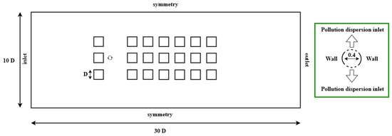
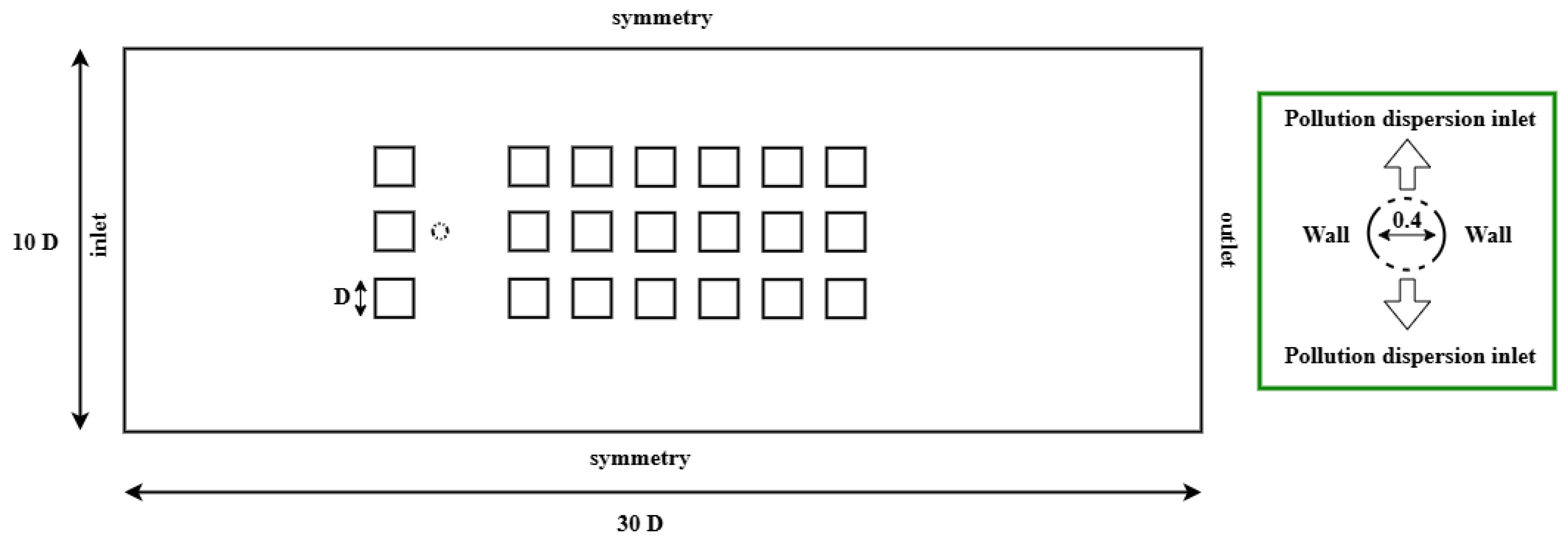
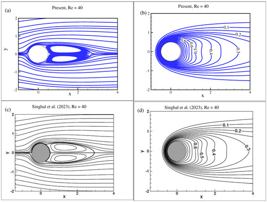
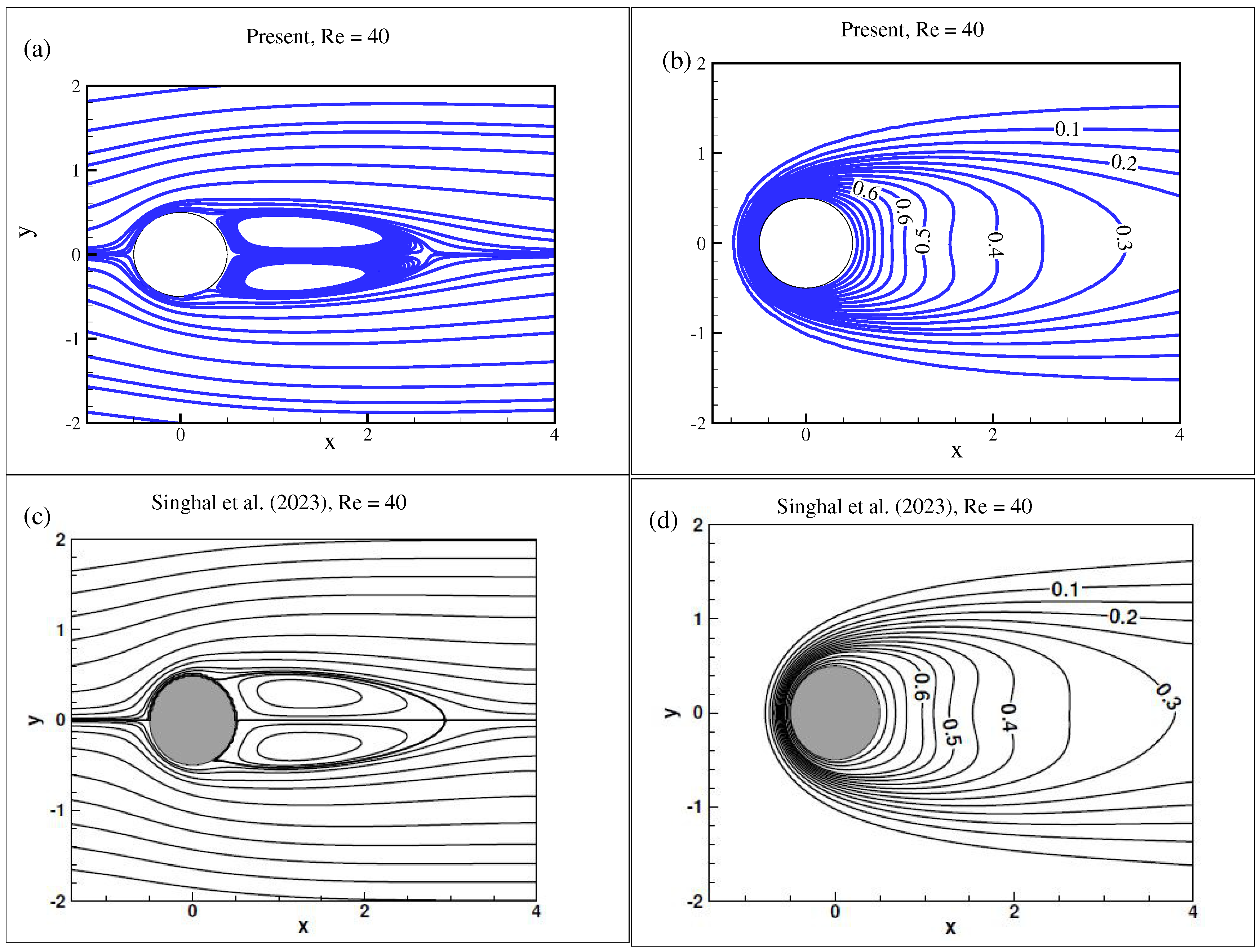
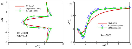
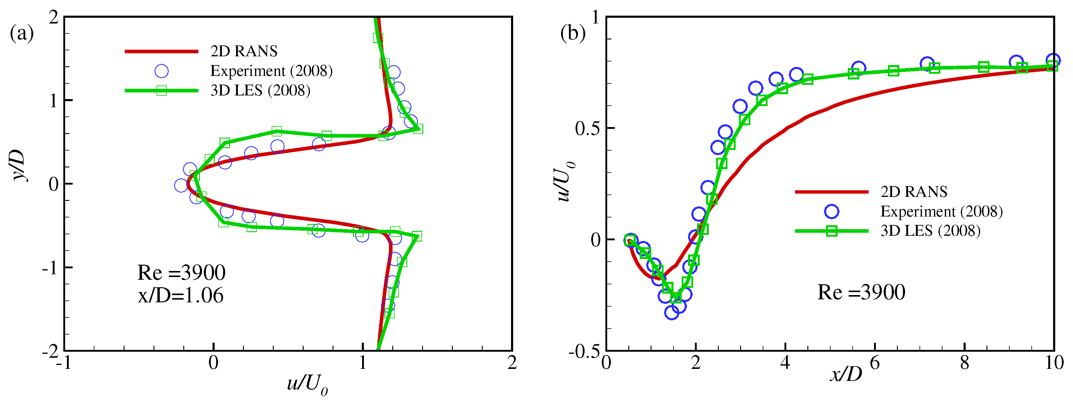
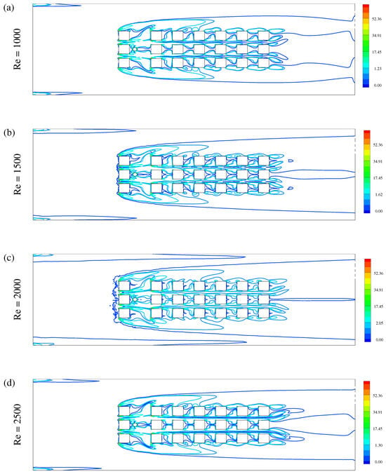
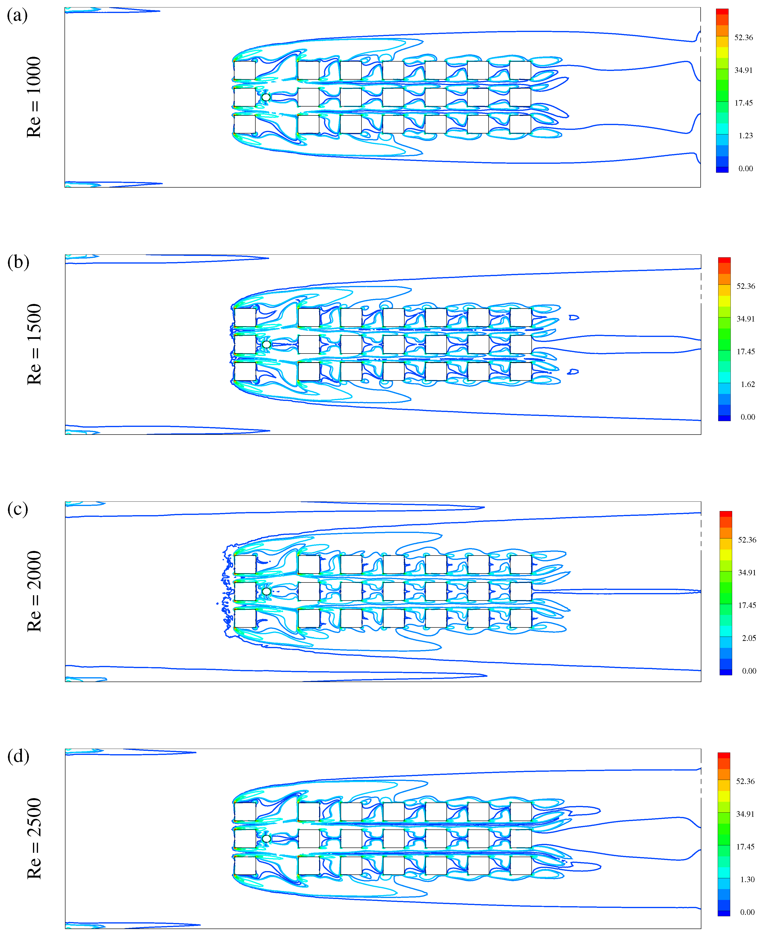
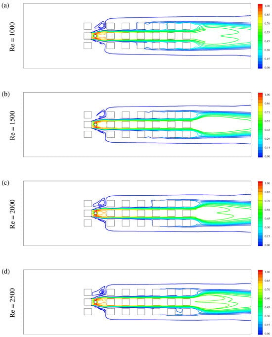
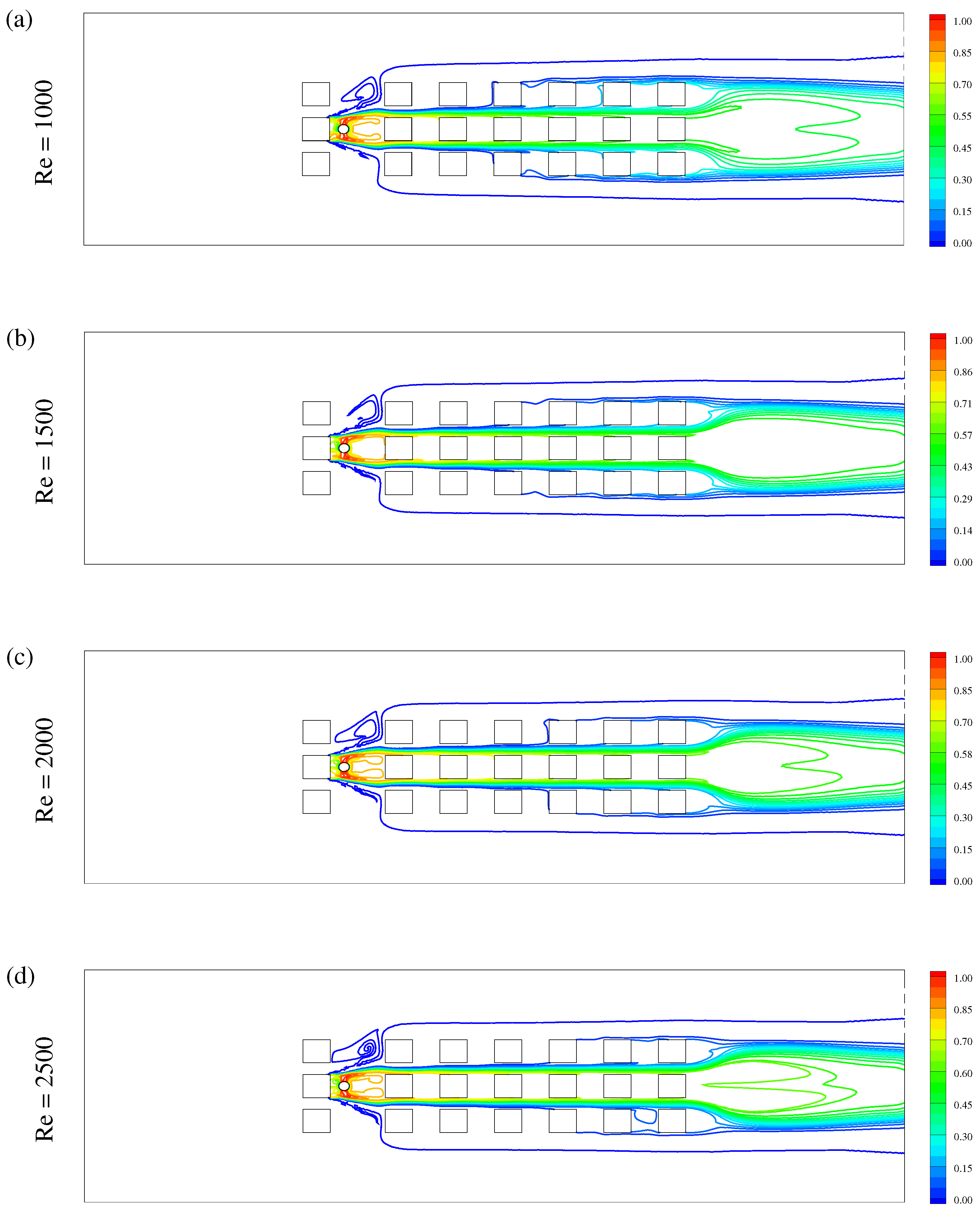
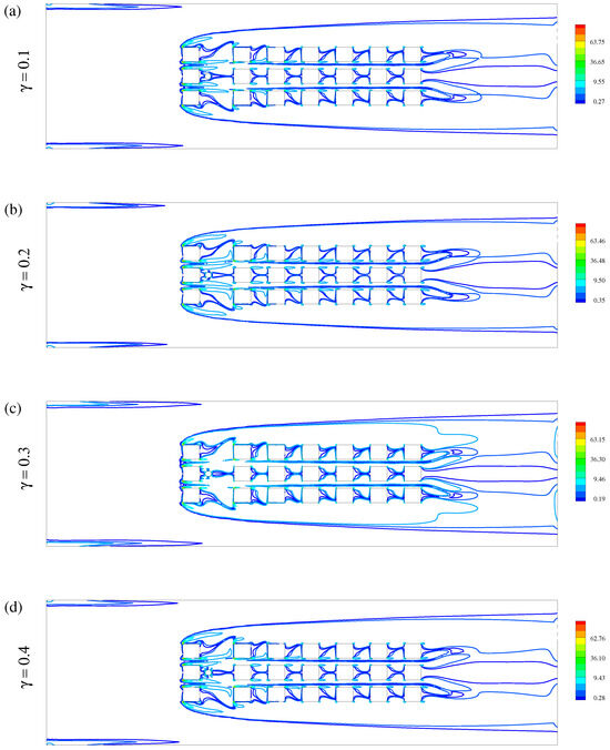
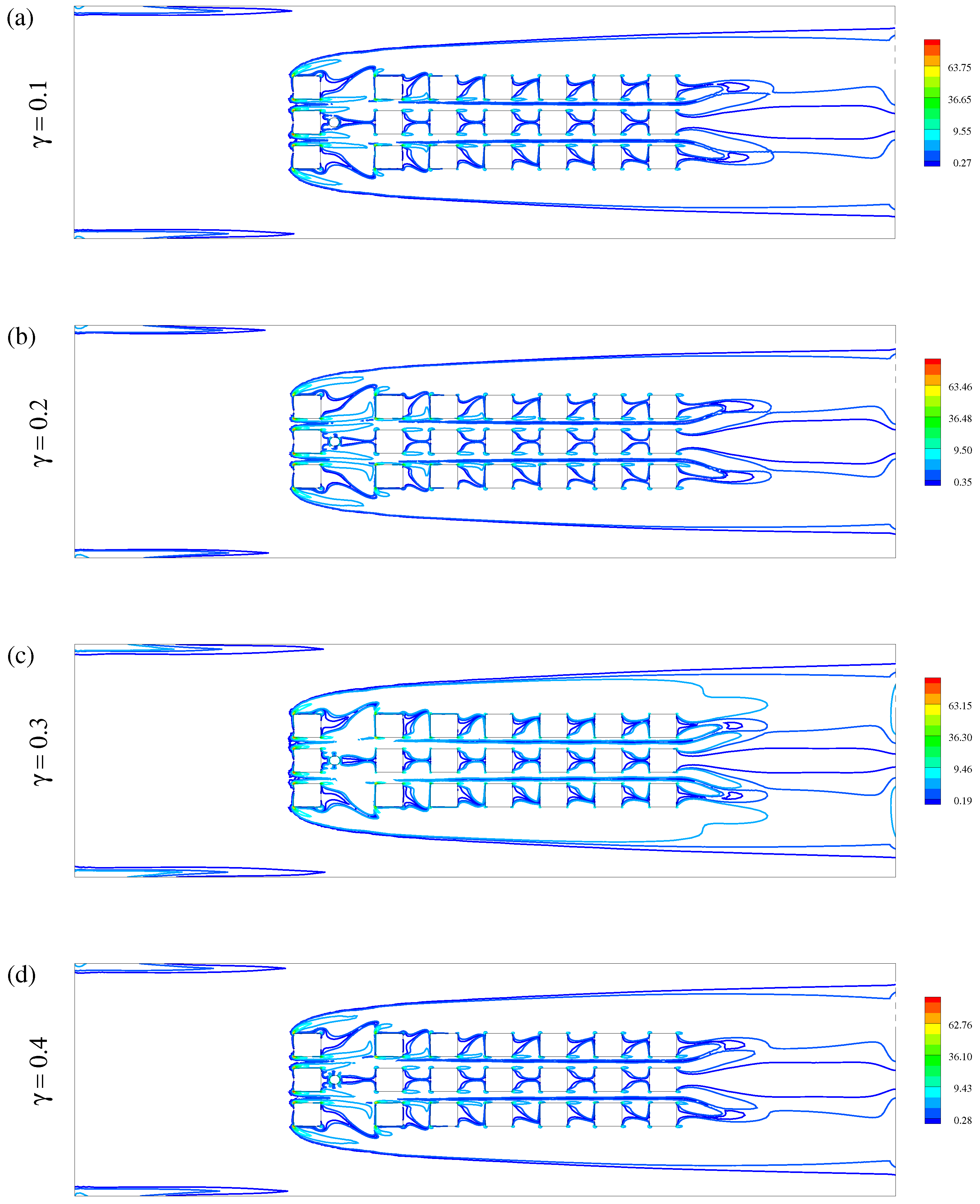
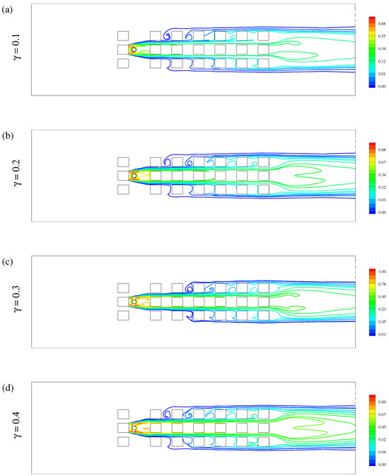
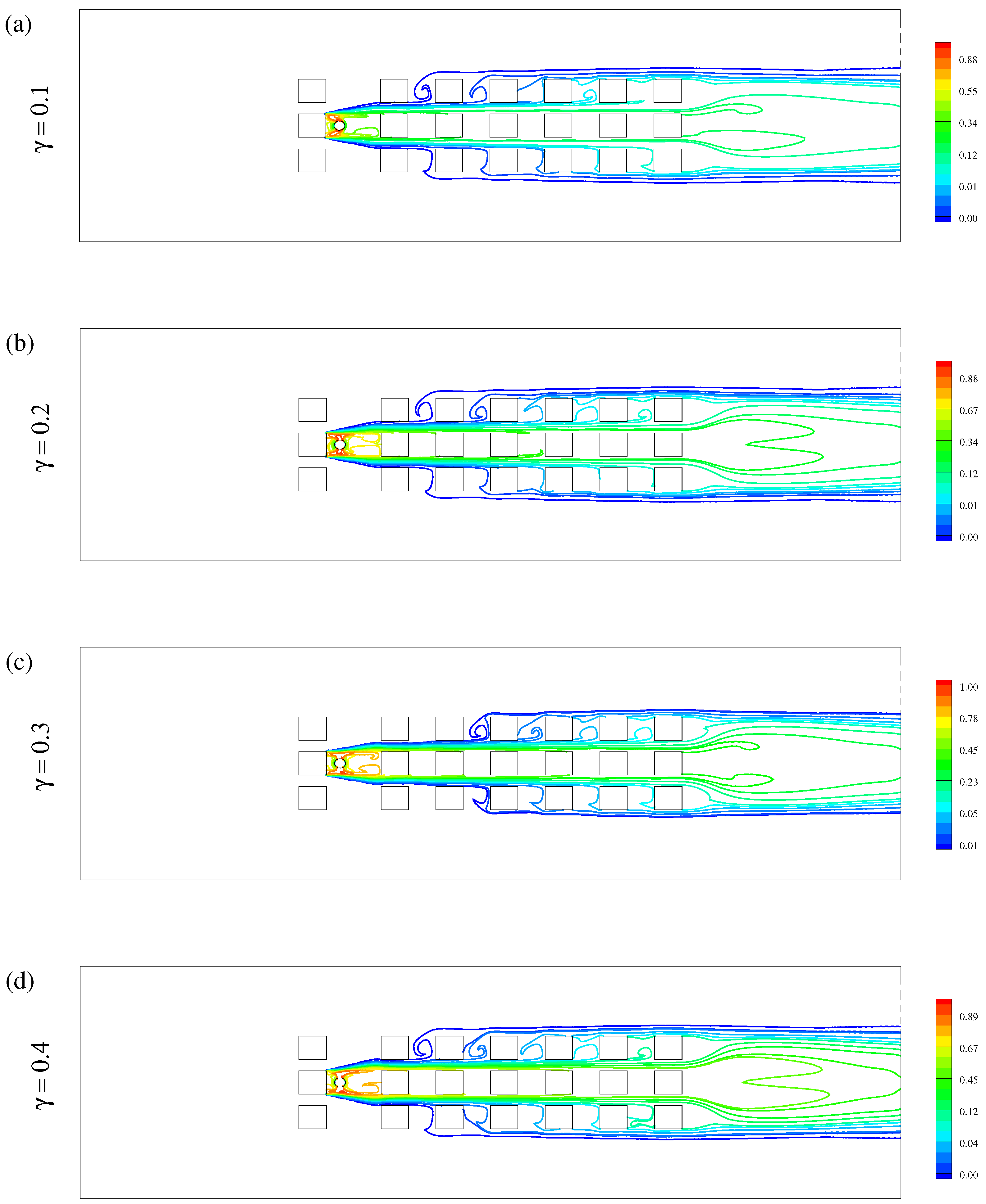
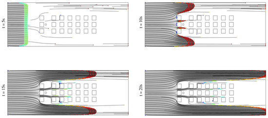
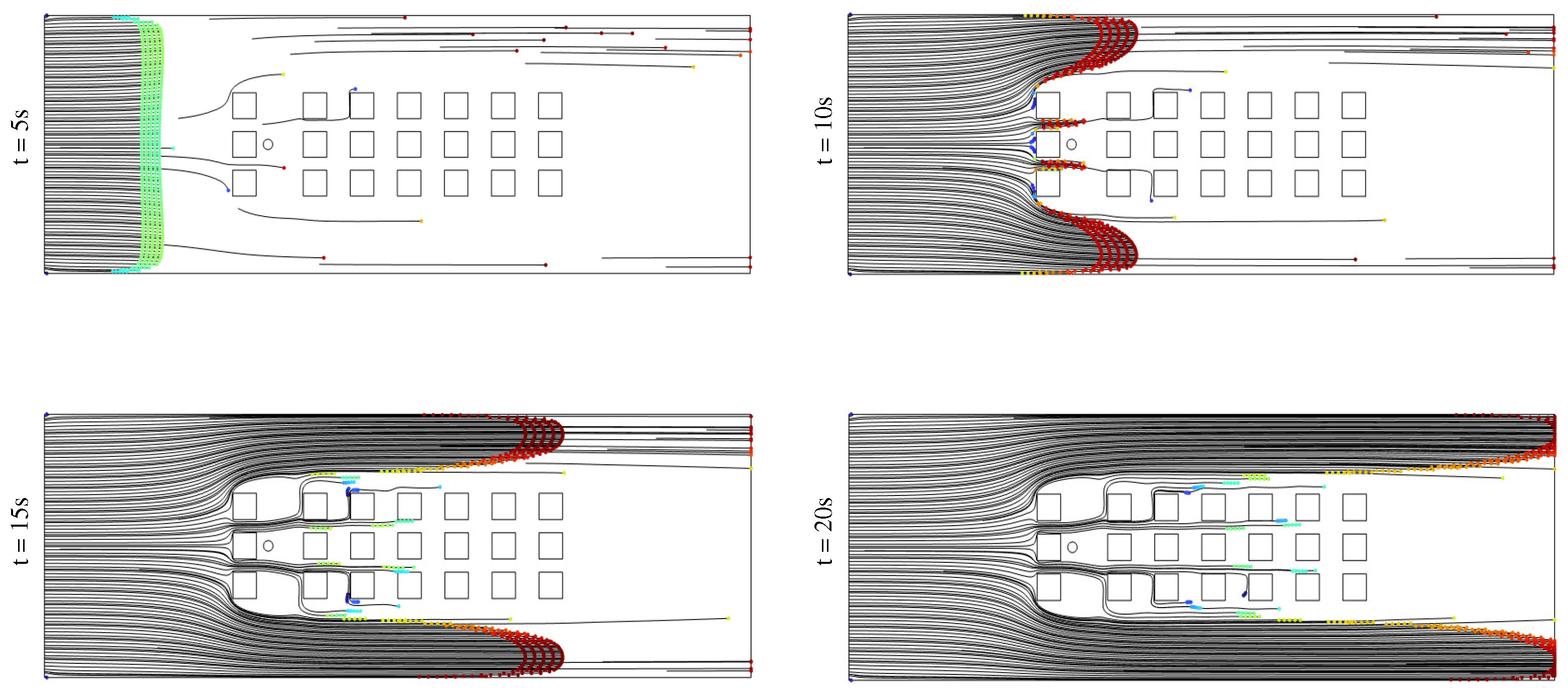
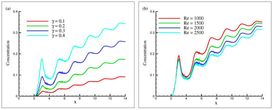
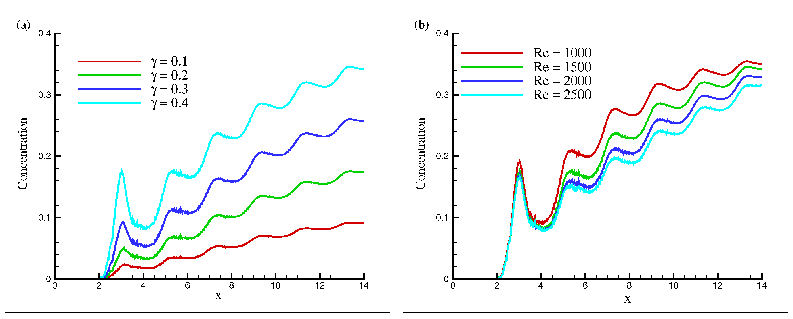
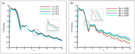
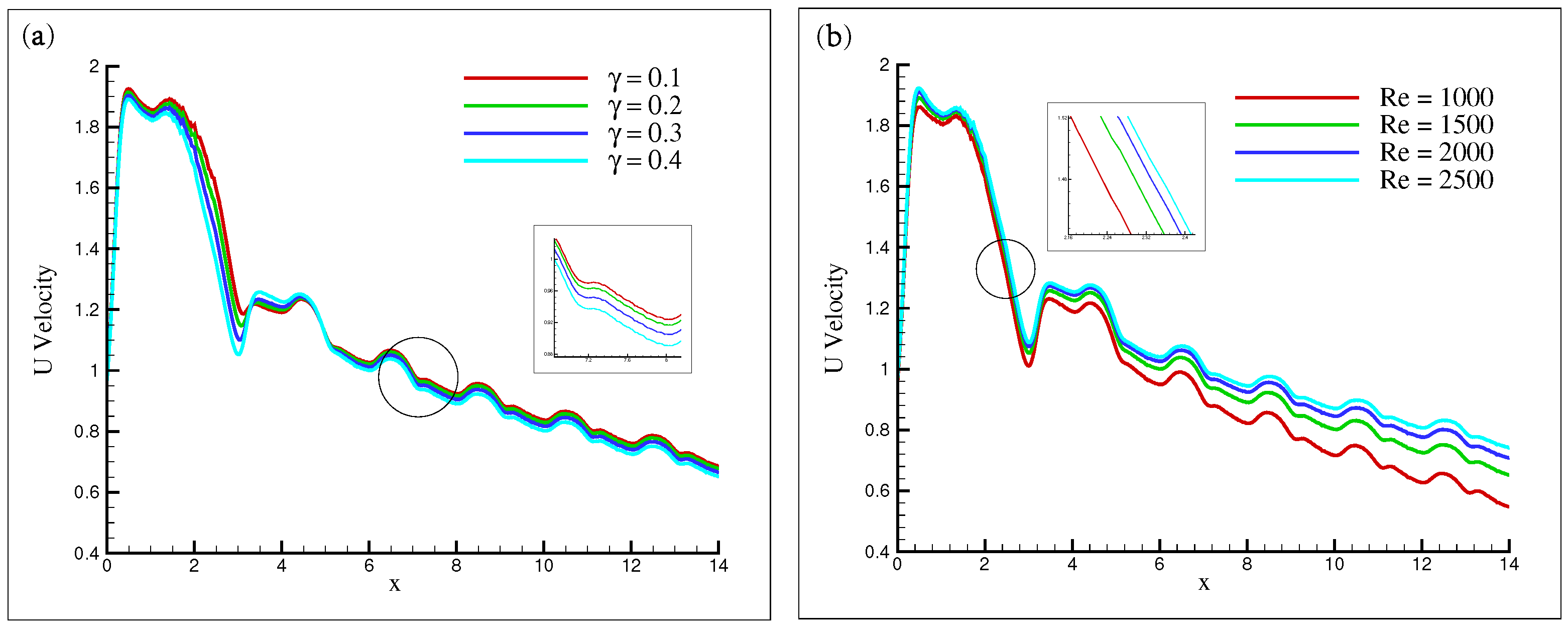
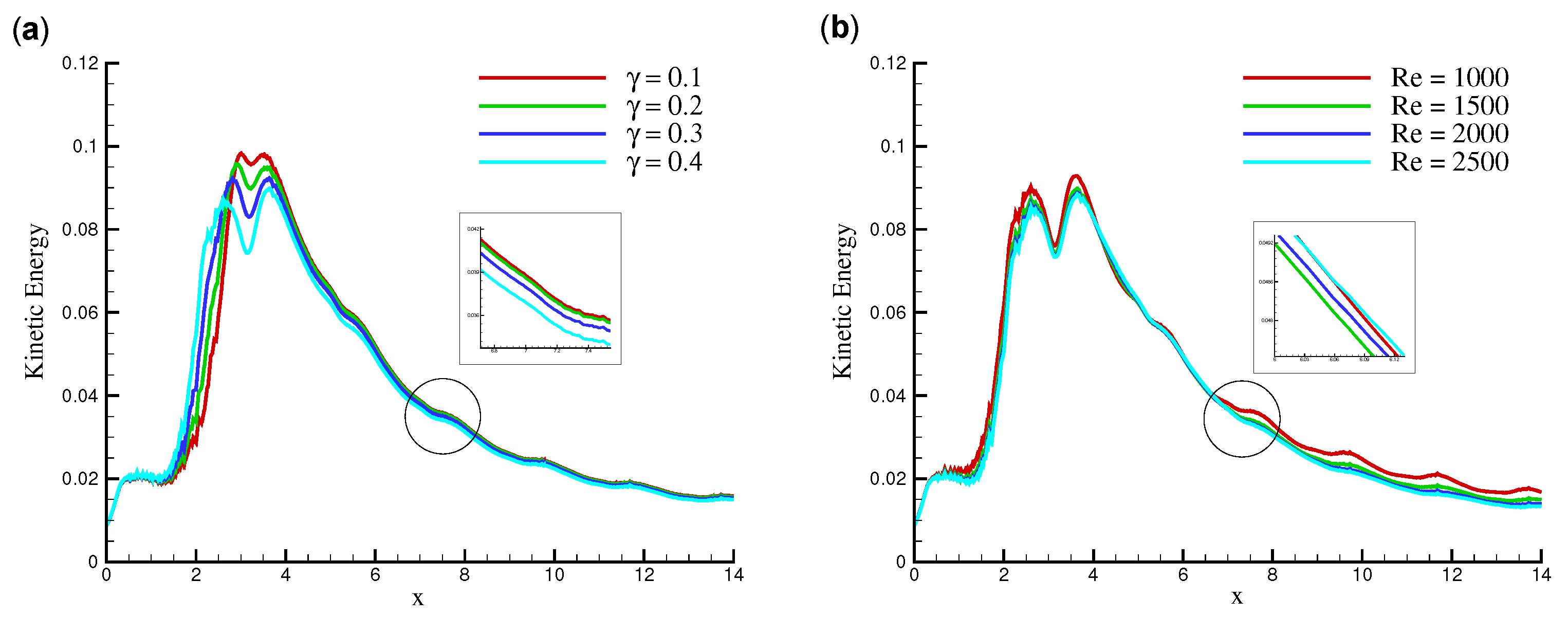
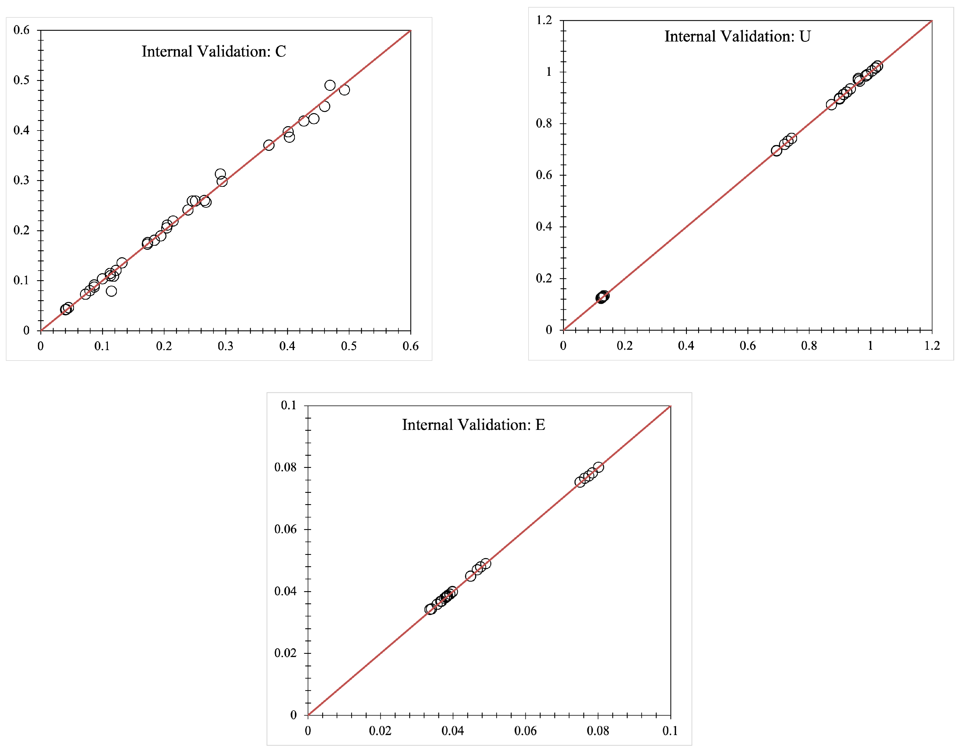
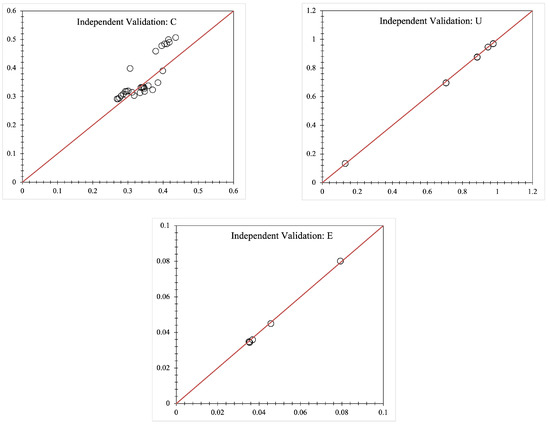
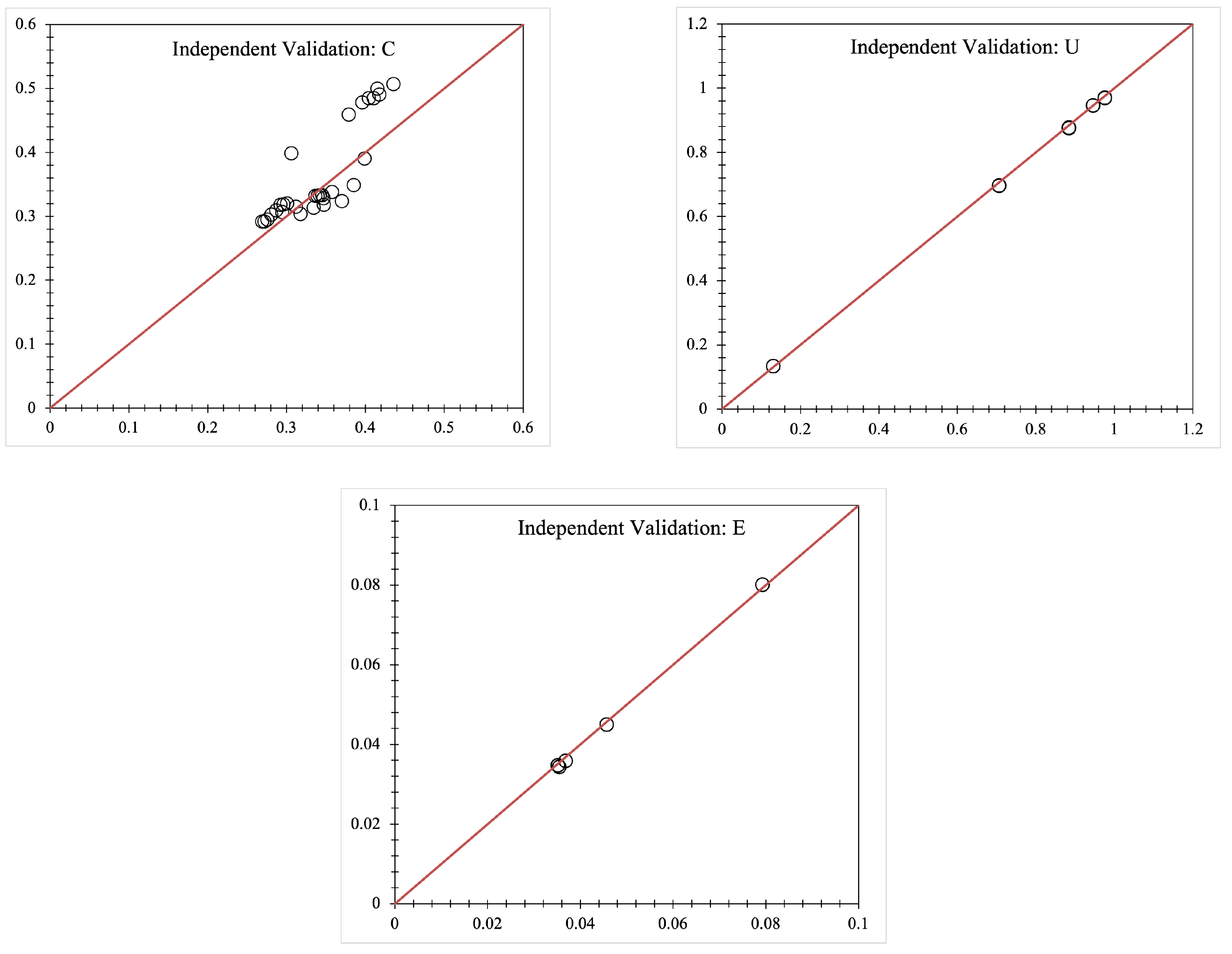
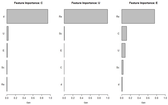
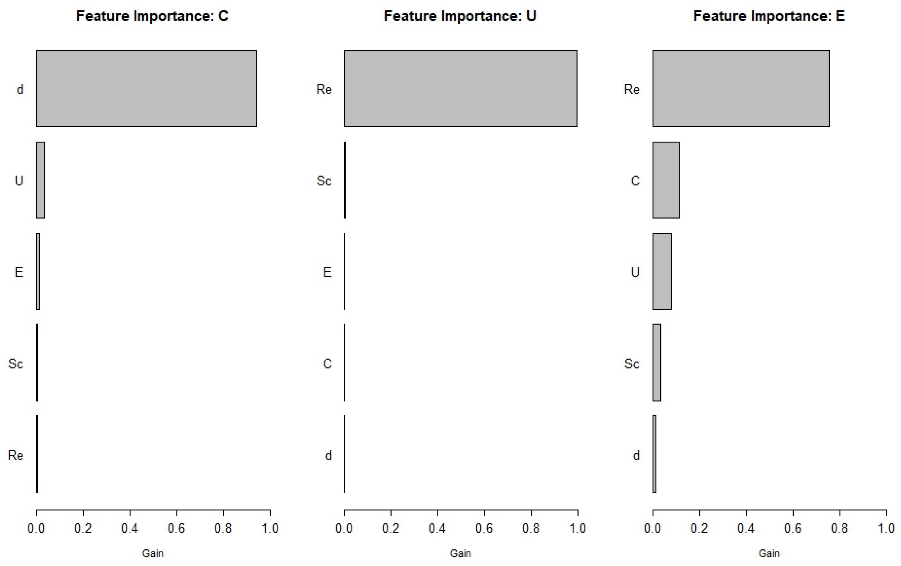

Disclaimer/Publisher’s Note: The statements, opinions and data contained in all publications are solely those of the individual author(s) and contributor(s) and not of MDPI and/or the editor(s). MDPI and/or the editor(s) disclaim responsibility for any injury to people or property resulting from any ideas, methods, instructions or products referred to in the content. |
© 2026 by the authors. Licensee MDPI, Basel, Switzerland. This article is an open access article distributed under the terms and conditions of the Creative Commons Attribution (CC BY) license.