A Novel l₁ Exact Penalty Function Method and Its Application

Abstract

Penalty function methods are fundamental for solving constrained optimization problems, yet the widely used $l_1$ exact penalty function is non-differentiable and therefore incompatible with gradient-based algorithms. This paper proposes a continuously differentiable smoothing approximation that preserves the exactness of the original penalty while enabling efficient numerical solution. The proposed smoothing function is shown to be ${\mathcal{C}}^1$ on $\mathbb{R}$, with explicit error bounds and a computable lower bound for the penalty parameter that guarantees exactness under standard constraint qualifications. An iterative algorithm is developed and its convergence is proved. Numerical experiments on benchmark problems validate the effectiveness of the approach. The method is then applied to a policy-driven university financial risk management model with twelve decision variables, three conflicting objectives, and multiple regulatory constraints. Results demonstrate faster convergence and improved objective values compared with the traditional non-smooth penalty method, confirming the practical utility of the proposed smoothing technique.

1. Introduction

Constrained optimization problems are widely applied in economics and public administration. The core methods for constrained optimization include Lagrangian approaches and penalty function methods. Among the various solution methodologies, the penalty function method is one of the most fundamental and widely used approaches, which transforms a constrained problem into an unconstrained one by adding a penalty term that penalizes constraint violations. The classical quadratic penalty method requires the penalty parameter to tend to infinity to recover the exact solution, often leading to ill-conditioned numerical subproblems. In contrast, the exact penalty function attains the true solution for a finite penalty parameter, thereby overcoming the numerical instability inherent in quadratic penalty methods. However, its non-differentiability at constraint boundaries prevents the direct use of gradient-based optimization algorithms.

Since Zangwill’s pioneering work [1], the development of exact penalty methods has evolved significantly. For continuously differentiable $f,g_i:{\mathbb{R}}^n\to \mathbb{R}$, the original inequality constrained problem reads

$$\begin{array}{cc}\hfill \left(P\right)\min & f\left(x\right)\hfill \\ \hfill \mathrm{s}.\mathrm{t}.& g_i\left(x\right)\le 0,i\in I,\hfill \end{array}$$

where $I=\{1,2,\dots ,m\}$. Let $p\left(t\right)=\max \{t,0\}$. The constraint violation term is uniformly written as $p\left(g_i\left(x\right)\right)$, and the feasible set is $X_0=\{x\in {\mathbb{R}}^n\mid g_i\left(x\right)⩽0,i\in I\}$. In 1967, Zangwill introduced the classical exact but non-differentiable $l_1$ penalty function:

$$F_1\left(x,\rho \right)=f\left(x\right)+\rho {\displaystyle \sum _{i=1}^m}p\left(g_i\left(x\right)\right),$$

which corresponds to unconstrained problem

$$\left(P_1\right)\min F_1\left(x,\rho \right),\mathrm{s}.\mathrm{t}.x\in {\mathbb{R}}^n.$$

Since then, a great deal of research has focused on various alternative formulations. Luo [2] developed a lower-order penalty approach:

$$f\left(x\right)+\alpha {\left({\displaystyle \sum _{i=1}^m}p\left(g_i\left(x\right)\right)\right)}^{{\displaystyle \frac{1}{\beta }}},$$

where $\alpha >0$ and $\beta >0$ are penalty parameters. The literature [3,4] investigated generalized nonlinear penalty functions:

$$L^k\left(x,d\right)={\left[f{\left(x\right)}^k+{\displaystyle \sum _{i=1}^m}{d}_i\left(p{\left(g_i\left(x\right)\right)}^k\right)\right]}^{{\displaystyle \frac{1}{k}}},$$

where $k>0$, $d=(d_1,d_2,\dots ,d_m)$ is the penalty parameter.

Wu [5] proposed a class of lower-order exact penalty functions:

$$F^k\left(x,\rho \right)=f\left(x\right)+\rho {\displaystyle \sum _{i=1}^m}{\left(p\left(g_i\left(x\right)\right)\right)}^k,$$

where $\rho$ is the penalty parameter and $k\in (0,1)$ represents the order of the lower-order penalty function. When $k=1$, it degenerates into the $l_1$ penalty function.

Although lower-order penalty functions with $k\in (0,1)$ can achieve exactness with smaller penalty parameters, their derivatives become unbounded as $g_i\left(x\right)\to 0^{+}$, which may cause numerical instability in gradient-based optimization. In contrast, the classical $l_1$ formulation has bounded derivatives and exhibits more stable numerical behavior, making it preferable for practical applications such as the financial risk management problem considered in this paper. We therefore focus on smoothing the $l_1$ exact penalty function.

Due to the non-differentiability of the $l_1$ penalty, scholars have developed multiple smoothing approximation techniques. Representative existing smoothing functions are listed as follows:

Liu [6] introduced a twice continuously differentiable piecewise exponential smoothing function:

$$p_{\epsilon }\left(t\right)=\left\{\begin{array}{cc}{\displaystyle \frac{1}{2}}\epsilon e^{{\displaystyle \frac{t}{\epsilon }}},& t<0,\\ t+{\displaystyle \frac{1}{2}}\epsilon e^{-{\displaystyle \frac{t}{\epsilon }}},& t>0.\end{array}\right.$$

Sood et al. [7] presented a power-based smoothing technique:

$$p_{\epsilon }\left(t\right)=\left\{\begin{array}{cc}0,& t<0,\\ {\displaystyle \frac{1}{2}}{t}^{{\displaystyle \frac{3}{2}}}{\epsilon }^{-{\displaystyle \frac{3}{4}}},& 0⩽t⩽\epsilon ,\\ t^{{\displaystyle \frac{3}{4}}}-{\displaystyle \frac{1}{2}}{\epsilon }^{{\displaystyle \frac{3}{4}}},& t⩾\epsilon .\end{array}\right.$$

Yilmaz and Zeytinoglu [8] put forward a rational smoothing function with second-order differentiability:

$$s_{\epsilon }\left(t\right)=\left\{\begin{array}{cc}0,& t<0,\\ {\displaystyle \frac{t^{p+4}}{t^4+{\epsilon }^4}},& t⩾0.\end{array}\right.$$

Considerable efforts have been devoted to smoothing the $l_1$ exact penalty function. Early works include Pinar and Zenios [9], who proposed a first-order differentiable smoothing approximation and established convergence relationships between the smoothed and original problems. Wu et al. [10] introduced a quadratic smoothing function and proved global convergence under standard assumptions. Liu [6] extended the idea to a family of twice-differentiable exponential smoothing functions. Lian [11] developed a piecewise cubic smoothing function with improved error bounds, while Xu and Dang [12] proposed a second-order smoothing function and demonstrated its numerical efficiency. Qiu et al. [13] further investigated a two-parameter smoothing framework with enhanced flexibility. Concurrently, several studies have explored smoothing techniques for lower-order exact penalty functions [14]. Despite these advances, most existing methods provide only qualitative or implicit estimates of the penalty parameter threshold, leaving practitioners without a clear guideline for choosing $\rho$ in real applications. Moreover, recent smoothing works have primarily targeted generic convex engineering optimization problems [15,16], while the non-convex, multi-coupled constraints arising in university financial systems have received less attention. It is acknowledged that the proposed smoothing function itself is an incremental development within the existing literature. Its distinguishing features are twofold: a computable lower bound for the penalty parameter under the LICQ condition, and the first application of a smoothing penalty method to a multi-constraint university financial risk optimization model. A piecewise ${\mathcal{C}}^1$ continuous smoothing approximation for the $l_1$ exact penalty function is constructed. Strict exactness conditions for the penalty parameter, including a computable lower bound under the mild assumption, are derived. The proposed algorithm is then applied to a multi-constraint university financial risk optimization model.

The remainder of this paper is organized as follows. Section 2 elaborates the proposed smoothed penalty function and its approximation properties. Section 3 designs the iterative algorithm and proves convergence. Section 4 conducts tests on standard optimization benchmarks. Section 5 establishes a multi-variable nonlinear financial model based on real regulatory rules and verifies algorithm performance. The last section concludes this work.

2. A Smoothing Penalty Function

To theoretically analyze the exactness property of the $l_1$ exact penalty function and lay a solid theoretical basis for the subsequent smoothing approximation design and algorithm improvement, two standard assumptions that will be enforced throughout this paper.

Assumption 1.

The objective function $f\left(x\right)$ is coercive, $i.e., {\lim }_{\parallel x\parallel \to \infty }f\left(x\right)=+\infty$.

This implies that all local minimizers of the original constrained optimization problem lie within a bounded compact set.

Assumption 2.

The original constrained optimization problem has only a finite number of local minimizers.

Under the above assumptions, the exact property of the penalty function can be guaranteed by selecting a sufficiently large penalty parameter. The original inequality-constrained optimization problem (P) can be equivalently transformed into an unconstrained optimization problem via the $l_1$ exact penalty strategy. For any given penalty parameter $\rho >0$, the optimization problem is formulated as

$$G(x,\rho )=f\left(x\right)+\rho {\displaystyle \sum _{i=1}^m}p\left(g_i\left(x\right)\right),$$

(1)

where $p\left(t\right)=\max \{t,0\}$.

The associated constrained problem is

$$\begin{array}{cc}\hfill \left(P_{\rho }\right)& \min G(x,\rho ),\mathrm{s}.\mathrm{t}.x\in {\mathbb{R}}^n.\hfill \end{array}$$

(2)

To approximate $p\left(t\right)$, a smoothed variant $p_{\epsilon }\left(t\right)$ parameterized by $\epsilon >0$ is introduced:

$$p_{\epsilon }\left(t\right)=\left\{\begin{array}{cc}0,& t<0,\\ {\displaystyle \frac{t^3}{3{\epsilon }^2}}+{\displaystyle \frac{t^2}{4\epsilon }},& 0\le t\le \epsilon ,\\ t-{\displaystyle \frac{1}{2}}\epsilon e^{-{\displaystyle \frac{t}{\epsilon }}+1}+{\displaystyle \frac{1}{12}}\epsilon ,& t>\epsilon ,\end{array}\right.$$

where $\epsilon$ controls the approximation accuracy and smoothness.

It can be obtained from $p_{\epsilon }\left(t\right)$ that

$$G_{\epsilon }(x,\rho )=f\left(x\right)+\rho {\displaystyle \sum _{i=1}^m}{p}_{\epsilon }\left(g_i\left(x\right)\right),$$

(3)

which yields the following smoothed penalty optimization problem:

$$\left(S{P}_{\rho ,\epsilon }\right)\min G_{\epsilon }\left(x,\rho \right),\mathrm{s}.\mathrm{t}.x\in {\mathbb{R}}^n.$$

(4)

When f is continuously differentiable, $G_{\epsilon }(x,\rho )$ inherits this property.

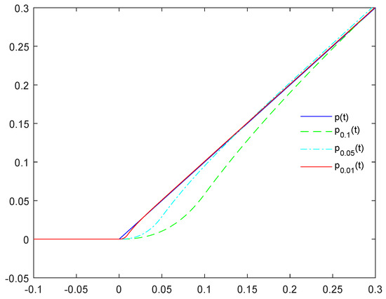
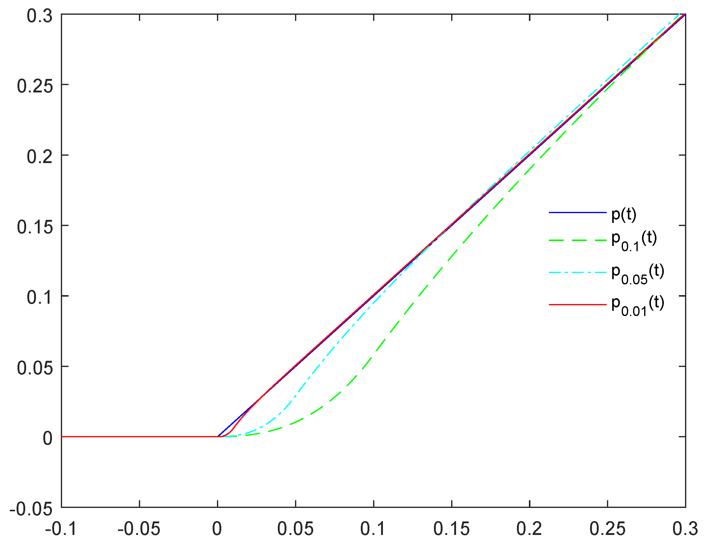
Figure 1 shows the curves of the original function $p\left(t\right)$ and the proposed smoothed function $p_{\epsilon }\left(t\right)$ with $\epsilon =0.1,0.05,0.01$. It can be observed that $p_{\epsilon }\left(t\right)$ gradually converges to the original non-smooth function $p\left(t\right)$ as $\epsilon$ decreases.

Figure 1. The figure of $p\left(t\right)$ and $p_{\epsilon }\left(t\right)$.

The following theorem gives the critical threshold of the penalty parameter.

Theorem 1.

Suppose that Assumptions 1 and 2 hold, $x^{\ast }$ is a local (or global) minimizer of the original constrained problem (P). There exists a threshold $\overline{\rho }>0$ such that for any penalty parameter $\rho \in (\overline{\rho },+\infty )$, every optimal solution to the unconstrained penalty problem is also an optimal solution to the original constrained problem.

Proof. 

The proof follows the standard exact penalty argument established in ([5], Corollary 2.3), with the key distinction that the boundedness of the penalty parameter threshold is ensured by the coercivity of $f\left(x\right)$ (Assumption 1) and the finiteness of local minimizers (Assumption 2). Under these assumptions, the argument proceeds by contradiction: if a minimizer of $G(x,\rho )$ were infeasible, the penalty term would grow without bound as $\rho \to \infty$, contradicting the optimality of $x^{\ast }$. Hence there exists a threshold $\overline{\rho }>0$ such that for any penalty parameter $\rho \in (\overline{\rho },+\infty )$, every optimal solution of the unconstrained penalty problem is feasible and optimal for the original constrained problem.    □

Corollary 1.

Suppose $x^{\ast }$ is a local minimizer of $\left(P\right)$ satisfying the Linear Independence Constraint Qualification (LICQ) at the active constraints. Let ${\lambda }_i\ge 0$ be the corresponding Lagrange multipliers for the active constraints $i\in I\left(x^{\ast }\right)=\{i\mid g_i\left(x^{\ast }\right)=0\}$. Then the threshold in Theorem 1 can be estimated as

$$\overline{\rho }>\underset{i\in I\left(x^{\ast }\right)}{\max }\left|{\lambda }_i\right|.$$

Proof. 

Under the LICQ assumption, the KKT conditions hold at $x^{\ast }$ with unique Lagrange multipliers ${\lambda }_i$ for $i\in I\left(x^{\ast }\right)$. As shown in the proof of Theorem 1, the penalty parameter threshold is determined by the magnitudes of these multipliers. Specifically, ([5], Remark 2.1) establishes that for a lower-order penalty function ${\varphi }_{\rho ,k}\left(x\right)=f\left(x\right)+\rho \sum \left[p\left(g_i\left(x\right)\right)\right]$, the second-order sufficiency condition implies local exact penalty property when $\rho >{\max }_{i}k{(f\left(x^{\ast }\right)+c)}^{k-1}{\lambda }_i$. For the classical $l_1$ penalty function, which corresponds to the case $k=1$ and $c=0$, this condition reduces to

$$\rho >\underset{i\in I\left(x^{\ast }\right)}{\max }\left|{\lambda }_i\right|.$$

Thus the threshold $\overline{\rho }$ in Theorem 1 can be taken as

$$\underset{i\in I\left(x^{\ast }\right)}{\max }\left|{\lambda }_i\right|.$$

   □

Remark 1.

The bound $\rho >{\max }_{i\in I\left(x^{\ast }\right)}\left|{\lambda }_i\right|$ has a natural interpretation: the penalty parameter must be large enough to dominate the largest Lagrange multiplier associated with the active constraints. Intuitively, if ρ is smaller than some $|{\lambda }_i|$, the cost of violating the $i\mathrm{th}$ constraint is cheaper than the reduction in the objective obtained by moving away from the constraint boundary, so the minimizer of the penalty problem would not satisfy the original constraint. Thus ρ must exceed the magnitude of all active Lagrange multipliers to ensure that constraint violations are never beneficial. This provides a practical guideline: one can estimate ρ by solving the KKT system locally, or use a conservative large value when such estimates are unavailable.

Remark 2.

The smoothed function $p_{\epsilon }\left(t\right)$ satisfies the properties:

(i) 

For any $\epsilon >0$, $p_{\epsilon }\left(t\right)$ is continuously differentiable with derivative:

$$p_{\epsilon }^{\prime }\left(t\right)=\left\{\begin{array}{cc}0,\hfill & t<0,\hfill \\ {\displaystyle \frac{t^2}{{\epsilon }^2}}+{\displaystyle \frac{t}{2\epsilon }},\hfill & 0⩽t⩽\epsilon ,\hfill \\ 1+{\displaystyle \frac{1}{2}}{e}^{1-t/\epsilon },\hfill & t>\epsilon .\hfill \end{array}\right.$$

(ii) 

It converges pointwise to the original penalty function: $\underset{\epsilon \to 0}{\lim }{p}_{\epsilon }\left(t\right)=p\left(t\right)$.

Proof. 

To verify that $p_{\epsilon }\left(t\right)$ is continuously differentiable on $\mathbb{R}$, it suffices to check the continuity of $p_{\epsilon }\left(t\right)$ and $p_{\epsilon }^{\prime }\left(t\right)$ at the junction points $t=0$ and $t=\epsilon$:

$$\begin{array}{cc}\hfill \underset{t\to 0^{-}}{\lim }{p}_{\epsilon }\left(t\right)& =\underset{t\to 0^{+}}{\lim }{p}_{\epsilon }\left(t\right)=0=p_{\epsilon }\left(0\right),\hfill \\ \hfill \underset{t\to 0^{-}}{\lim }{p}_{\epsilon }^{\prime }\left(t\right)& =\underset{t\to 0^{+}}{\lim }{p}_{\epsilon }^{\prime }\left(t\right)=0=p_{\epsilon }^{\prime }\left(0\right),\hfill \\ \hfill \underset{t\to {\epsilon }^{-}}{\lim }{p}_{\epsilon }\left(t\right)& =\underset{t\to {\epsilon }^{+}}{\lim }{p}_{\epsilon }\left(t\right)=\frac{7}{12}\epsilon =p_{\epsilon }\left(\epsilon \right),\hfill \\ \hfill \underset{t\to {\epsilon }^{-}}{\lim }{p}_{\epsilon }^{\prime }\left(t\right)& =\underset{t\to {\epsilon }^{+}}{\lim }{p}_{\epsilon }^{\prime }\left(t\right)=\frac{3}{2}=p_{\epsilon }^{\prime }\left(\epsilon \right).\hfill \end{array}$$

These limits confirm $p_{\epsilon }$ is ${\mathcal{C}}^1$ for all $\epsilon >0$.

The pointwise convergence follows from:

$$\underset{\epsilon \to 0}{\lim }{p}_{\epsilon }\left(t\right)=\left\{\begin{array}{cc}0=p\left(t\right),\hfill & t<0,\hfill \\ 0=p\left(t\right),\hfill & t=0,\hfill \\ t=p\left(t\right),\hfill & t>0.\hfill \end{array}\right.$$

where the $t=0$ case uses $\underset{\epsilon \to 0}{\lim }\left({\displaystyle \frac{t^3}{3{\epsilon }^2}}+{\displaystyle \frac{t^2}{4\epsilon }}\right)=0$ and the $t>0$ case follows from $\underset{\epsilon \to 0}{\lim }\left(t-{\displaystyle \frac{1}{2}}\epsilon e^{-{\displaystyle \frac{t}{\epsilon }}+1}+{\displaystyle \frac{1}{12}}\epsilon \right)=t$.    □

Definition 1 

([17]). For any $\epsilon >0$, a point $x_{\epsilon }\in {\mathbb{R}}^n$ is called an ε-feasible solution to $\left(P\right)$ if

$$g_i\left(x_{\epsilon }\right)⩽\epsilon ,\forall i\in I$$

(5)

Definition 2 

([17]). Let $f^{\ast }$ be the optimal objective value of $\left(P\right)$. For any $\epsilon >0$, a point $x_{\epsilon }\in X_0$ is called an ε-approximate optimal solution to $\left(P\right)$ if

$$\left|f^{\ast }-f\left(x_{\epsilon }\right)\right|⩽\epsilon .$$

Next, the error estimates are analyzed.

Theorem 2.

For any given positive constants ε and ρ,

$$-{\displaystyle \frac{1}{12}}m\rho \epsilon <G\left(x,\rho \right)-G_{\epsilon }\left(x,\rho \right)⩽{\displaystyle \frac{5}{12}}m\rho \epsilon ,\forall x\in {\mathbb{R}}^n.$$

(6)

Proof. 

For all $x\in {\mathbb{R}}^n$ and $i\in I$, it can be obtained from $p\left(t\right)$ and $p_{\epsilon }\left(t\right)$ that

$$p\left(g_i\left(x\right)\right)-p_{\epsilon }\left(g_i\left(x\right)\right)=\left\{\begin{array}{cc}0,\hfill & g_i\left(x\right)<0,\hfill \\ g_i\left(x\right)-{\displaystyle \frac{{\left(g_i\left(x\right)\right)}^3}{3{\epsilon }^2}}-{\displaystyle \frac{{\left(g_i\left(x\right)\right)}^2}{4\epsilon }},\hfill & 0⩽g_i\left(x\right)⩽\epsilon ,\hfill \\ {\displaystyle \frac{1}{2}}\epsilon e^{-{\displaystyle \frac{g_i\left(x\right)}{\epsilon }}+1}-{\displaystyle \frac{1}{12}}\epsilon ,\hfill & g_i\left(x\right)>\epsilon .\hfill \end{array}\right.$$

(7)

Then for each $i\in I$,

$$-{\displaystyle \frac{1}{12}}\epsilon <p\left(g_i\left(x\right)\right)-p_{\epsilon }\left(g_i\left(x\right)\right)⩽{\displaystyle \frac{5}{12}}\epsilon .$$

(8)

It can be derived by summing over i from 1 to m that

$$-{\displaystyle \frac{1}{12}}m\epsilon <{\displaystyle \sum _{i=1}^m}p\left(g_i\left(x\right)\right)-{\displaystyle \sum _{i=1}^m}{p}_{\epsilon }\left(g_i\left(x\right)\right)⩽{\displaystyle \frac{5}{12}}m\epsilon .$$

Hence,

$$-{\displaystyle \frac{1}{12}}m\rho \epsilon <\rho {\displaystyle \sum _{i=1}^m}p\left(g_i\left(x\right)\right)-\rho {\displaystyle \sum _{i=1}^m}{p}_{\epsilon }\left(g_i\left(x\right)\right)⩽{\displaystyle \frac{5}{12}}m\rho \epsilon .$$

This completes the proof.    □

Theorem 3.

Let ${\epsilon }_j$ be a sequence of positive numbers converging to 0. Assume $x_j$ is a solution to the minimization problem $\underset{x\in {\mathbb{R}}^n}{\min }{G}_{{\epsilon }_j}\left(x,\rho \right)$ for some $\rho >0$. If $x_{\epsilon }$ is an accumulation point of the sequence $\left\{x_j\right\}$, then $x_{\epsilon }$ is an optimal solution to the minimization problem $\underset{x\in {\mathbb{R}}^n}{\min }G\left(x,\rho \right)$.

Proof. 

Let x be any point in ${\mathbb{R}}^n$. Since $x_j$ minimizes $G_{{\epsilon }_j}\left(·,\rho \right)$, ones have

$$G_{{\epsilon }_j}\left(x_j,\rho \right)\le G_{{\epsilon }_j}\left(x,\rho \right).$$

Taking the limit $j\to \infty$ on both sides, and using the pointwise convergence $G_{{\epsilon }_j}\left(x,\rho \right)\to G\left(x,\rho \right)$ established in Remark 2, yields

$$G\left(x_{\epsilon },\rho \right)\le G\left(x,\rho \right)$$

for all $x\in {\mathbb{R}}^n$. Hence $x_{\epsilon }$ is a global minimizer of $G\left(x,\rho \right)$.    □

Theorem 4.

Let $x^{\ast }$ and $x_{\epsilon }$ be optimal solutions to $\left(P_{\rho }\right)$ and $\left(S{P}_{\rho ,\epsilon }\right)$ respectively for some $\rho >0$. Then

$$-{\displaystyle \frac{1}{12}}m\rho \epsilon <G\left(x^{\ast },\rho \right)-G_{\epsilon }\left(x_{\epsilon },\rho \right)⩽{\displaystyle \frac{5}{12}}m\rho \epsilon .$$

(9)

Proof. 

According to Theorem 2, it can be derived from $\rho >0$ that

$$-{\displaystyle \frac{1}{12}}m\rho \epsilon <G\left(x^{\ast },\rho \right)-G_{\epsilon }\left(x^{\ast },\rho \right)⩽{\displaystyle \frac{5}{12}}m\rho \epsilon$$

(10)

and

$$-{\displaystyle \frac{1}{12}}m\rho \epsilon <G\left(x_{\epsilon },\rho \right)-G_{\epsilon }\left(x_{\epsilon },\rho \right)⩽{\displaystyle \frac{5}{12}}m\rho \epsilon .$$

(11)

Since $x^{\ast }$ and $x_{\epsilon }$ are optimal solutions to $\left(P_{\rho }\right)$ and $\left(S{P}_{\rho ,\epsilon }\right)$, respectively, then

$$G\left(x^{\ast },\rho \right)⩽G\left(x_{\epsilon },\rho \right)\mathrm{and}{G}_{\epsilon }\left(x_{\epsilon },\rho \right)⩽G_{\epsilon }\left(x^{\ast },\rho \right).$$

These, together with (10) and (11), give

$$\begin{array}{cc}\hfill -{\displaystyle \frac{1}{12}}m\rho \epsilon & <G(x^{\ast },\rho )-G_{\epsilon }(x^{\ast },\rho )\hfill \\ \hfill & ⩽G(x^{\ast },\rho )-G_{\epsilon }(x_{\epsilon },\rho )\hfill \\ \hfill & ⩽G(x_{\epsilon },\rho )-G_{\epsilon }(x_{\epsilon },\rho )\hfill \\ \hfill & ⩽{\displaystyle \frac{5}{12}}m\rho \epsilon .\hfill \end{array}$$

(12)

This completes the proof.    □

3. A New Smoothing Algorithm

In this section, a penalty function algorithm for addressing problem $\left(P\right)$ is developed, closely linked to the smooth penalty problem $\left(S{P}_{\rho ,\epsilon }\right)$ established in the preceding discussion.

Remark 3.

In practical implementations, the subproblem ${\min }_{x\in {\mathbb{R}}^n}{G}_{{\epsilon }_j}\left(x,{\rho }_j\right)$ can be solved using any standard gradient-based optimization solver, terminated when the gradient norm falls below a specified tolerance ${\tau }_j$, i.e., $\parallel \nabla G_{{\epsilon }_j}(x,\rho )\parallel \le {\tau }_j$, where ${\tau }_j$ is set to $max\{{\epsilon }_j,1\times {10}^{-6}\}$. The initial penalty parameter ${\rho }_0$ is chosen moderately to avoid ill-conditioning at early iterations. The update factors $N>1$ and $0<\delta <1$ are selected to balance convergence speed and approximation accuracy: a larger N accelerates constraint satisfaction but may cause instability, while a smaller δ improves smoothness approximation but increases the number of iterations. In the numerical experiments, these parameters are tuned on a case-by-case basis, as reported in Section 4.

Remark 4.

Under Algorithm 1 with parameters $N>1$ and $0<\delta <1$, the parameter sequences satisfy ${\epsilon }_j\to 0$ and ${\rho }_j\to +\infty$ as $j\to \infty$.

Algorithm 1 A penalty function algorithm
	Step 1: Initialize $x_0$, with $\epsilon >0$, ${\epsilon }_0>0$, ${\rho }_0>0$, $0<\delta <1$, and $N>1$. Then, set $j=0$ and move to Step 2;
	Step 2: Starting from $x_j$, solve the problem $$\left(S{P}_{{\rho }_j,{\epsilon }_j}\right)\underset{x\in {\mathbb{R}}^n}{\min }{G}_{{\epsilon }_j}\left(x,{\rho }_j\right)=f\left(x\right)+{\rho }_j{\displaystyle \sum _{i=1}^m}{p}_{{\epsilon }_j}\left(g_i\left(x\right)\right)$$ and obtain a stationary point $x_{j+1}$ satisfying $\nabla G_{{\epsilon }_j}(x_{j+1},{\rho }_j)=0$;
	Step 3: If $x_{j+1}$ is $\epsilon$-feasible to $\left(P\right)$, terminate the process. Otherwise, update the parameters with ${\rho }_{j+1}=N{\rho }_j$, ${\epsilon }_{j+1}=\delta {\epsilon }_j$, and $j=j+1$, and return to Step 2.

In practical implementations, exact minimization $x_j\in \arg \underset{x\in {\mathbb{R}}^n}{\min }{G}_{{\epsilon }_j}(x,{\rho }_j)$ is computationally challenging. Instead, seek a local minimizer or stationary point $x_{j+1}$ satisfying the first-order optimality condition $\nabla G_{{\epsilon }_j}(x_{j+1},{\rho }_j)=0$.

As illustrated in Remark 4, ${\rho }_j\to +\infty$ as $j\to \infty$. Nevertheless, all feasible regions of the constrained optimization problems considered in this paper, ranging from standard numerical examples to the university financial risk model, are closed and bounded. In view of the non-negativity of $p_{\epsilon }\left(t\right)$, the sequence $\left\{G_{{\epsilon }_j}(x_j,{\rho }_j)\right\}$ remains uniformly bounded even when the penalty parameter tends to infinity. Accordingly, the boundedness condition in Theorem 5 holds for all test problems studied in this work.

To characterize the constraint activity, set the index set I as follows:

• $I_{\epsilon }^{+}\left(x\right)=\{i\in I\mid g_i\left(x\right)\ge \epsilon \}$
• $I_{\epsilon }^{-}\left(x\right)=\{i\in I\mid g_i\left(x\right)<0\}$
• $I_{\epsilon }^{+-}\left(x\right)=\{i\in I\mid 0\le g_i\left(x\right)\le \epsilon \}$

Theorem 5.

Let $\underset{\parallel x\parallel \to +\infty }{\lim }f\left(x\right)=+\infty$ and $\left\{x_j\right\}$ be the sequence generated by Algorithm 1. If $\left\{G_{{\epsilon }_j}(x_j,{\rho }_j)\right\}$ is bounded, then

(a) 

$\left\{x_j\right\}$ is bounded;

(b) 

Any limit point $x^{\ast }$ of $\left\{x_j\right\}$ is feasible for $\left(P\right)$;

(c) 

There exist positive constants λ and ${\mu }_i\ge 0$ ($i=1,\dots ,m$) such that $x^{\ast }$ satisfies

$$\lambda \nabla f\left(x^{\ast }\right)+{\displaystyle \sum _{i=1}^m}{\mu }_i\nabla g_i\left(x^{\ast }\right)=0.$$

(13)

Proof. 

Assume that the sequence $\left\{G_{{\epsilon }_j}(x_j,{\rho }_j)\right\}$ is bounded, i.e., there exists a positive constant L such that

$$G_{{\epsilon }_j}(x_j,{\rho }_j)⩽L,j=0,1,2,\dots .$$

(14)

Suppose, for the sake of contradiction, that $\left\{x_j\right\}$ is unbounded. Without loss of generality, assume that $\underset{j\to +\infty }{\lim }\parallel x_j\parallel =+\infty$. From the definition of $p_{\epsilon }\left(t\right)$, ones have

$${\displaystyle \sum _{i=1}^m}{p}_{{\epsilon }_j}\left(g_i\left(x_j\right)\right)⩾0.$$

(15)

Therefore,

$$L⩾G_{{\epsilon }_j}(x_j,{\rho }_j)=f\left(x_j\right)+{\rho }_j\sum _{i\in I}{p}_{{\epsilon }_j}\left(g_i\left(x_j\right)\right)⩾f\left(x_j\right),$$

which contradicts $\underset{\parallel x\parallel \to +\infty }{\lim }f\left(x\right)=+\infty$. Hence, $\left\{x_j\right\}$ is bounded.

Without loss of generality, assume $x_j\to x^{\ast }$. Suppose, to the contrary, that $x^{\ast }$ is infeasible for $\left(P\right)$. Then there exists $i_0\in I$ such that $g_{i_0}\left(x^{\ast }\right)>0$. By continuity,

$$\underset{j\to \infty }{\lim }{g}_{i_0}\left(x_j\right)=g_{i_0}\left(x^{\ast }\right)>0.$$

A simple calculation gives

$$\begin{array}{cc}\hfill G_{{\epsilon }_j}(x_j,{\rho }_j)=& f\left(x_j\right)+{\rho }_j\sum _{i\in I_{{\epsilon }_j}^{+}\left(x_j\right)}\left({\displaystyle \frac{g_i^3\left(x_j\right)}{3{\epsilon }_j^2}}+{\displaystyle \frac{g_i^2\left(x_j\right)}{4{\epsilon }_j}}\right)\hfill \\ \hfill & +{\rho }_j\sum _{i\in I_{{\epsilon }_j}^{+-}\left(x_j\right)}\left(g_i\left(x_j\right)-{\displaystyle \frac{1}{2}}{\epsilon }_j{e}^{-{\displaystyle \frac{g_i\left(x_j\right)}{{\epsilon }_j}}+1}+{\displaystyle \frac{1}{12}}{\epsilon }_j\right).\hfill \end{array}$$

(16)

It follows that $\underset{j\to +\infty }{\lim }{G}_{{\epsilon }_j}(x_j,{\rho }_j)=+\infty$, a contradiction.

From part (b), $x^{\ast }\in X$, so $g_i\left(x^{\ast }\right)⩽0$ for all $i\in I$. There exist $\lambda ⩾0$ and ${\mu }_i⩾0$ such that

$$\lambda \nabla f\left(x^{\ast }\right)+\sum _{i\in I}{\mu }_i\nabla g_i\left(x^{\ast }\right)=0.$$

By Step 2 of Algorithm 1, $\nabla G_{{\epsilon }_j}(x_j,{\rho }_j)=0$, so

$$\begin{array}{cc}\hfill & \nabla f\left(x_j\right)+{\rho }_j\sum _{i\in I_{{\epsilon }_j}^{+}\left(x_j\right)}\left({\displaystyle \frac{g_i^2\left(x_j\right)}{{\epsilon }_j^2}}+{\displaystyle \frac{g_i\left(x_j\right)}{2{\epsilon }_j}}\right)\nabla g_i\left(x_j\right)\hfill \\ \hfill & +{\rho }_j\sum _{i\in I_{{\epsilon }_j}^{+-}\left(x_j\right)}\left(1+{\displaystyle \frac{1}{2}}{e}^{-{\displaystyle \frac{g_i\left(x_j\right)}{{\epsilon }_j}}+1}\right)\nabla g_i\left(x_j\right)=0.\hfill \end{array}$$

(17)

For each j, define

$$\begin{array}{cc}\hfill {\gamma }_j& =1+{\rho }_j\sum _{i\in I_{{\epsilon }_j}^{+}\left(x_j\right)}\left({\displaystyle \frac{g_i^2\left(x_j\right)}{{\epsilon }_j^2}}+{\displaystyle \frac{g_i\left(x_j\right)}{2{\epsilon }_j}}\right)\hfill \\ \hfill & +{\rho }_j\sum _{i\in I_{{\epsilon }_j}^{+-}\left(x_j\right)}\left(1+{\displaystyle \frac{1}{2}}{e}^{-{\displaystyle \frac{g_i\left(x_j\right)}{{\epsilon }_j}}+1}\right).\hfill \end{array}$$

(18)

Clearly ${\gamma }_j>1$. Dividing (17) by ${\gamma }_j$,

$$\begin{array}{cc}\hfill & {\displaystyle \frac{\nabla f\left(x_j\right)}{{\gamma }_j}}+{\displaystyle \frac{{\rho }_j}{{\gamma }_j}}\sum _{i\in I_{{\epsilon }_j}^{+}\left(x_j\right)}\left({\displaystyle \frac{g_i^2\left(x_j\right)}{{\epsilon }_j^2}}+{\displaystyle \frac{g_i\left(x_j\right)}{2{\epsilon }_j}}\right)\nabla g_i\left(x_j\right)\hfill \\ \hfill & +{\displaystyle \frac{{\rho }_j}{{\gamma }_j}}\sum _{i\in I_{{\epsilon }_j}^{+-}\left(x_j\right)}\left(1+{\displaystyle \frac{1}{2}}{e}^{-{\displaystyle \frac{g_i\left(x_j\right)}{{\epsilon }_j}}+1}\right)\nabla g_i\left(x_j\right)=0.\hfill \end{array}$$

(19)

Let

$${\lambda }_j={\displaystyle \frac{1}{{\gamma }_j}},$$

$${\mu }_i^j=\left\{\begin{array}{cc}{\displaystyle \frac{{\rho }_j}{{\gamma }_j}}\left({\displaystyle \frac{g_i^2\left(x_j\right)}{{\epsilon }_j^2}}+{\displaystyle \frac{g_i\left(x_j\right)}{2{\epsilon }_j}}\right),\hfill & i\in I_{{\epsilon }_j}^{+}\left(x_j\right),\hfill \\ {\displaystyle \frac{{\rho }_j}{{\gamma }_j}}\left(1+{\displaystyle \frac{1}{2}}{e}^{-{\displaystyle \frac{g_i\left(x_j\right)}{{\epsilon }_j}}+1}\right),\hfill & i\in I_{{\epsilon }_j}^{+-}\left(x_j\right),\hfill \\ 0,\hfill & i\in I\setminus \left(I_{{\epsilon }_j}^{+}\left(x_j\right)\cup I_{{\epsilon }_j}^{+-}\left(x_j\right)\right).\hfill \end{array}\right.$$

Then

$${\lambda }_j+\sum _{i\in I}{\mu }_i^j=1,{\mu }_i^j⩾0.$$

(20)

Taking convergent subsequences, ${\lambda }_j\to \lambda ⩾0$, ${\mu }_i^j\to {\mu }_i⩾0$. Passing to the limit in (19),

$$\lambda \nabla f\left(x^{\ast }\right)+\sum _{i\in I}{\mu }_i\nabla g_i\left(x^{\ast }\right)=0,\lambda +\sum _{i\in I}{\mu }_i=1.$$

For inactive constraints $i\in I\setminus I\left(x^{\ast }\right)$, ones have ${\mu }_i=0$. Thus the KKT conditions hold.

This completes the proof. □

The boundedness of $\left\{G_{{\epsilon }_j}(x_j,{\rho }_j)\right\}$ is guaranteed if the feasible set is nonempty and compact and f is bounded below. For any feasible $\overline{x}$, optimality of $x_j$ gives $G_{{\epsilon }_j}\left(x_j,{\rho }_j\right)<G_{{\epsilon }_j}\left(\overline{x},{\rho }_j\right)=f\left(\overline{x}\right)$, since $p_{{\epsilon }_j}\left(g_i\left(\overline{x}\right)\right)=0$ for sufficiently small ${\epsilon }_j$. Thus the sequence is bounded above by $f\left(\overline{x}\right)$, independent of j. This condition holds for all test problems in this study.

4. Numerical Examples

The algorithm’s implementation in MATLAB R2022A is presented in this section, followed by a discussion of numerical results that demonstrate its effectiveness. Before evaluating the proposed method on practical problems, its numerical performance is first assessed on four standard benchmark problems that are widely used in the constrained optimization literature. These examples serve to validate the algorithm’s solution accuracy and numerical stability in generic constrained optimization settings, providing a reliable basis for assessing its fundamental capabilities.

Detailed outcomes are presented in tables, where specific symbols are used for brevity. In these tables, j denotes the iteration number, $x_j$ is the local minimum point at iteration j, ${\rho }_j$ is the penalty function parameter, $g_i\left(x_j\right)$ indicates the constraint function’s value evaluated at $x_j$, and $f\left(x_j\right)$ corresponds to the value of the local minimum point $x_j$ under the objective function f.

Example 1.

Consider example $\left(COP1\right)$, as presented in [11].

$$\begin{array}{cc}\hfill \min & f\left(x\right)=x_1^2+x_2^2+2x_3^2+x_4^2-5x_1-5x_2-21x_3+7x_4\hfill \\ \hfill \mathrm{s}.\mathrm{t}.& g_1\left(x\right)=2x_1^2+x_2^2+x_3^2+2x_1+x_2+x_4-5\le 0,\hfill \\ & g_2\left(x\right)=x_1^2+x_2^2+x_3^2+x_4^2+x_1-x_2+x_3-x_4-8\le 0,\hfill \\ & g_3\left(x\right)=x_1^2+2x_2^2+x_3^2+2x_4^2-x_1-x_4-10\le 0.\hfill \end{array}$$

Table 1 presents the numerical results of Algorithm 1 applied to $\left(COP1\right)$, with the initial condition set as $x_0=(1,1,1,1)$, ${\rho }_0=5$, $N=1$, ${\epsilon }_0=0.05$, $\delta =0.05$, and $\epsilon ={10}^{-6}$. As can be seen from the table, the approximate global solution obtained is $x^{\ast }=(0.16958,0.83556,2.00860,-0.96490)$, in just three iterations, achieving an objective function value of $-44.23390$.

Table 1. Results of Algorithm 1 with $x_0=(1,1,1,1)$, ${\rho }_0=5$, $N=1$.

j	${\mathit{\rho }}_{\mathit{j}}$	${\mathit{\epsilon }}_{\mathit{j}}$	$\mathit{f}\left({\mathit{x}}_{\mathit{j}}\right)$	${\mathit{g}}_1\left({\mathit{x}}_{\mathit{j}}\right)$	${\mathit{g}}_2\left({\mathit{x}}_{\mathit{j}}\right)$	${\mathit{g}}_3\left({\mathit{x}}_{\mathit{j}}\right)$	${\mathit{x}}_{\mathit{j}}$
1	5	0.05	$-44.26261$	0.01048	0.16226	$-1.69266$	$(0.17019,0.83586,$ $2.01122,-0.96735)$
2	5	0.0025	$-44.23412$	0.00078	0.00018	$-1.88262$	$(0.16950,0.83559,$ $2.00866,-0.96491)$
3	5	0.000125	$-44.23383$	$-0.00005$	$-0.00006$	$-1.88309$	$(0.16958,0.83556,$ $2.00860,-0.96490)$

When compared to the existing literature, the superiority of the optimal value derived from Algorithm 1 in this study becomes evident. Ref. [11] reports an approximate global solution of $x^{\ast }=(0.1684621,0.8529065,2.000167,-0.9755604)$, yielding an objective function value of $-44.23040$. Similarly, [18] achieves an approximate global solution of $x^{\ast }=(0.170768,0.827977,2.011779,-0.960639)$ with a corresponding objective function value of $-44.233515$. The optimal value in this paper is also better than the optimal value in [18]. Further, the solution presented in [13], the obtained approximate global solution is $x^{\ast }=(0.1712,0.8317,2.0097,-0.9632)$, results in an objective function value of $-44.2338$. The optimal value in this paper is also better than the optimal value in [13]. The proposed algorithm consistently surpasses these results, achieving a superior optimal value in the aforementioned references.

Example 2.

For illustration, examine example $\left(COP2\right)$ from [10].

$$\begin{array}{cc}\hfill \min & f\left(x\right)=-2x_1-6x_2+x_1^2-2x_1{x}_2+2x_2^2\hfill \\ \hfill \mathrm{s}.\mathrm{t}.& g_1\left(x\right)=x_1+x_2\le 2,\hfill \\ & g_2\left(x\right)=-x_1+2x_2\le 2,\hfill \\ & x_1,x_2\ge 0.\hfill \end{array}$$

Numerical results for solving problem $\left(COP2\right)$ using Algorithm 1, initiated at $x_0=(1,1)$ and parameterized by ${\rho }_0=5$, $N=10$, ${\epsilon }_0=0.05$, $\delta =0.005$, and termination tolerance $\epsilon ={10}^{-6}$, are provided in Table 2. The resulting approximate global optimum, $x^{\ast }=(0.80005,1.19995)$, yields an objective function value of $-7.20000$. This result aligns with the optimal value $f\left(x^{\ast }\right)=-7.200000$ reported in [18].

Table 2. Results of Algorithm 1 with $x_0=(1,1)$, ${\rho }_0=5$, $N=10$.

j	${\mathit{\rho }}_{\mathit{j}}$	${\mathit{\epsilon }}_{\mathit{j}}$	$\mathit{f}\left({\mathit{x}}_{\mathit{j}}\right)$	${\mathit{g}}_1\left({\mathit{x}}_{\mathit{j}}\right)$	${\mathit{g}}_2\left({\mathit{x}}_{\mathit{j}}\right)$	${\mathit{x}}_{\mathit{j}}$
1	5	0.05	$-7.24410$	0.02687	$-0.39453$	$(0.81609,1.21078)$
2	50	0.00025	$-7.20034$	0.00021	$-0.39983$	$(0.80009,1.20013)$
3	500	0.00000125	$-7.20000$	0.00000	$-0.40015$	$(0.80005,1.19995)$

Example 3.

Examine $\left(COP3\right)$ from [11].

$$\begin{array}{cc}\hfill \min & f\left(x\right)=x_1^2+x_2^2-\cos \left(17x_1\right)-\cos \left(17x_2\right)+3\hfill \\ \hfill \mathrm{s}.\mathrm{t}.& g_1\left(x\right)={(x_1-2)}^2+x_2^2-1.6^2\le 0,\hfill \\ & g_2\left(x\right)=x_1^2+{(x_2-3)}^2-2.7^2\le 0,\hfill \\ & 0\le x_1\le 2,0\le x_2\le 2.\hfill \end{array}$$

As detailed in Table 3, Algorithm 1 accurately solves $\left(COP3\right)$ using initial conditions $x_0=(1,1)$, ${\rho }_0=12$, $N=10$, ${\epsilon }_0=0.05$, $\delta =0.001$, and $\epsilon ={10}^{-6}$. The algorithm converges to an approximate global optimum, $x^{\ast }=(0.72537,0.39926)$, providing an objective value of $1.83754$, demonstrating good agreement with the value reported in [11] where $f\left(x^{\ast }\right)=1.837623$. Furthermore, the proposed algorithm achieves a superior optimal value compared to the solution $x^{\ast }=(0.72608,0.39946)$ with corresponding objective function value $1.8376$ presented in [13].

Table 3. Results of Algorithm 1 with $x_0=(1,1)$, ${\rho }_0=12$, $N=10$.

j	${\mathit{\rho }}_{\mathit{j}}$	${\mathit{\epsilon }}_{\mathit{j}}$	$\mathit{f}\left({\mathit{x}}_{\mathit{j}}\right)$	${\mathit{g}}_1\left({\mathit{x}}_{\mathit{j}}\right)$	${\mathit{g}}_2\left({\mathit{x}}_{\mathit{j}}\right)$	${\mathit{x}}_{\mathit{j}}$
1	12	0.01	$1.837359$	$-0.77598$	$-1.92693$	$(0.72539,0.39923)$
2	120	0.00005	$1.83754$	$-0.77593$	$-1.92686$	$(0.72538,0.39926)$
3	1200	0.00000005	$1.83754$	$-0.77590$	$-1.92685$	$(0.72537,0.39926)$

Example 4.

Apply the proposed method to example $\left(COP4\right)$ discussed in [19].

$$\begin{array}{cc}\hfill \min & f\left(x\right)=x_1^2+x_1{x}_2+2x_2^2-6x_1-14x_2-12x_3\hfill \\ \hfill \mathrm{s}.\mathrm{t}.& g_1\left(x\right)=x_1+x_2+x_3=20,\hfill \\ & g_2\left(x\right)=x_1+2x_2\le 30,\hfill \\ & x_1,x_2,x_3\ge 0.\hfill \end{array}$$

Table 4 presents numerical results of Algorithm 1 for solving $\left(COP4\right)$ using initial conditions $x_0=(1,1,1)$, ${\rho }_0=10$, $N=2$, ${\epsilon }_0=0.01$ and $\delta =0.05$. The obtained approximate global solution $x^{\ast }=(0.00000,0.50002,19.49999)$ yields an objective function value of $-240.50010$, slightly better than the $-240.20$ reported in [19].

Table 4. Results of Algorithm 1 with $x_0=(1,1,1)$, ${\rho }_0=10$, $N=2$.

j	${\mathit{\rho }}_{\mathit{j}}$	${\mathit{\epsilon }}_{\mathit{j}}$	$\mathit{f}\left({\mathit{x}}_{\mathit{j}}\right)$	${\mathit{g}}_1\left({\mathit{x}}_{\mathit{j}}\right)$	${\mathit{g}}_2\left({\mathit{x}}_{\mathit{j}}\right)$	${\mathit{x}}_{\mathit{j}}$
1	10	0.01	$-240.50276$	0.00056	$-28.99981$	$(0.00001,0.50009,19.50046)$
2	20	0.0005	$-240.50010$	0.00000	$-28.99996$	$(0.00000,0.50002,19.49999)$

The four examples above demonstrate that the proposed smoothing $l_1$ exact penalty algorithm consistently achieves superior optimal values compared to existing methods in the literature, with fast convergence within a few iterations. These results confirm the algorithm’s fundamental numerical reliability and computational efficiency. In the following section, its practical performance is further evaluated on the university financial risk management model, which involves multiple financial decision variables, various categories of regulatory constraints, and a multi-objective optimization structure. This extension serves to validate the algorithm’s applicability in real-world financial risk control scenarios.

The numerical results above consistently show that the proposed smoothing function achieves competitive or better accuracy and faster convergence compared with existing methods. This behavior can be attributed to the structural properties of the smoothing function $p_{\epsilon }\left(t\right)$. In the transition region $0<t\le \epsilon$, the cubic polynomial ${\displaystyle \frac{t^3}{3{\epsilon }^2}}+{\displaystyle \frac{t^2}{4\epsilon }}$ provides a smooth transition from the flat region $t\le 0$ to the approximately linear growth region $t>\epsilon$. The derivative $p_{\epsilon }^{\prime }\left(t\right)$ is continuous and bounded across the junction points, which prevents numerical oscillations during gradient-based optimization. The exponential tail $t-{\displaystyle \frac{1}{2}}\epsilon e^{-{\displaystyle \frac{t}{\epsilon }}+1}+{\displaystyle \frac{1}{12}}\epsilon$ for $t>\epsilon$ ensures that the smoothed penalty closely tracks the original $l_1$ penalty for large constraint violations, preserving the exactness property of the original formulation. These features collectively explain the improved performance observed in the numerical experiments.

5. Application in University Financial Risk Optimization

With the rapid expansion of higher education in China, universities have continuously scaled up their operations, funding sources have diversified, and financial activities have become increasingly sophisticated. The financial management of universities—covering budget allocation, fund utilization, debt control, and resource deployment—is subject to multiple constraints including budget caps, debt limits, and regulatory requirements. The core objective is to minimize comprehensive financial risks while satisfying all these constraints. From the perspective of optimization theory, university financial risk management can be naturally formulated as a nonlinear constrained optimization problem. The smoothed $l_1$ exact penalty algorithm proposed in this paper is employed to solve this model, which not only validates the practical performance of the algorithm but also provides a scientific quantitative basis for precise financial risk control and optimal resource allocation in universities.

Building upon the validated algorithmic performance in Section 4, this section constructs a comprehensive nonlinear optimization model tailored to university financial risk management. The model incorporates domain-specific variables, multiple objectives, and complex constraints that reflect real regulatory and operational realities, thereby testing the algorithm’s capability in practical application environments.

University financial risks originate from multiple interrelated factors: excessive budget adjustments disrupt capital planning, long-term idle research funds reduce resource efficiency, and excessive debt increases repayment pressure and operational instability. Since simple linear models fail to capture the intricate relationships among risk indicators, this paper develops a quadratic nonlinear constrained optimization model grounded in the actual financial context of public universities. The model integrates linear inequalities, equality constraints, and bilateral bounds, which closely align with the multi-level supervision, risk interaction, and rigid financial balance characteristic of university finance. Through comparative experiments against traditional $l_1$ penalty algorithms, the feasibility, effectiveness, and practicality of the proposed method are comprehensively verified in terms of iteration count, optimal objective value, and other performance metrics.

5.1. Definition of Decision Variables

Twelve decision variables are defined, corresponding to twelve core financial risk dimensions: budget management, capital project implementation, debt risk prevention, fund operation, research fund utilization, state-owned asset administration, income structure, debt structure, liquidity management, investment stability, and personnel cost control. All indicators are normalized to the interval $[0,1]$ and satisfy the non-negativity condition $x_i\ge 0$, $i=1,2,\dots ,12$.

• $x_1$: Budget adjustment ratio, the proportion of adjusted funds to the total project budget, used to evaluate the standardization of budget formulation and execution;
• $x_2$: Unfinished ratio of capital projects, reflecting the lagging progress of infrastructure construction and large-scale equipment procurement;
• $x_3$: Illegal financing risk coefficient, measuring the risk of unauthorized loans and disguised debt financing;
• $x_4$: Ratio of overdue carry-over and surplus funds, representing fiscal funds that fail to be disposed within the required time limit;
• $x_5$: Idle ratio of special research funds, describing long-term unused research fiscal funds with low utilization efficiency;
• $x_6$: Idle ratio of state-owned assets, the proportion of idle fixed assets and large scientific instruments, which serves as a key indicator in asset performance evaluation;
• $x_7$: Fiscal funding dependency, the ratio of government fiscal allocation to total revenue, reflecting the university’s reliance on public budgets;
• $x_8$: Social donation and self-raised income ratio, the proportion of non-fiscal income in total revenue, measuring the diversification of funding sources;
• $x_9$: Short-term debt ratio, the proportion of debt maturing within one year to total debt, indicating the urgency of debt repayment pressure;
• $x_{10}$: Current ratio, the ratio of current assets to current liabilities, serving as a key indicator of short-term solvency;
• $x_{11}$: Investment return volatility coefficient, measuring the fluctuation of investment returns and the stability of financial assets;
• $x_{12}$: Personnel expenditure ratio, the proportion of personnel expenditure to total expenditure, reflecting the structure of university expenditure.

5.2. Objective Function

The optimization objective is to minimize the comprehensive financial risk of universities. Considering the mutual coupling among various risk indicators, a weighted quadratic function with cross-coupling terms is established. Based on expert evaluation widely adopted in university financial supervision, the weights of the first six single indicators are set as ${\omega }_1=0.24$, ${\omega }_2=0.20$, ${\omega }_3=0.22$, ${\omega }_4=0.16$, ${\omega }_5=0.12$, ${\omega }_6=0.06$; the coupling weight between any two of these indicators is uniformly set to ${\omega }_{ij}=0.02$ ($i<j$). For the six newly added variables, the single-indicator weights are set as ${\omega }_7=0.10$, ${\omega }_8=0.06$, ${\omega }_9=0.08$, ${\omega }_{10}=0.06$, ${\omega }_{11}=0.04$, ${\omega }_{12}=0.04$; the coupling weight between any two indicators is uniformly set to ${\omega }_{ij}=0.01$ ($i<j$). The financial risk minimization objective is formulated as

$$\min F_1\left(\mathbf{x}\right)={\displaystyle \sum _{i=1}^{12}}{\omega }_i{x}_i^2+\sum _{1\le i<j\le 12}{\omega }_{ij}{x}_i{x}_j.$$

(21)

In addition to risk minimization, universities must also pursue efficient fund utilization and financial sustainability. These three objectives are inherently conflicting: reducing debt risk may limit investment opportunities, while maximizing efficiency may increase short-term volatility.

Objective 2 (Fund utilization efficiency maximization):

$$\max F_2\left(\mathbf{x}\right)={\alpha }_1(1-x_2-x_4-x_5-x_6)+{\alpha }_2{x}_8+{\alpha }_3{\displaystyle \frac{1}{1+x_{11}}},$$

(22)

where the first term reflects the actual utilization rate of funds (deducting idle and delayed portions), the second term reflects income diversification, and the third term reflects investment stability. The weights are set as ${\alpha }_1=0.5$, ${\alpha }_2=0.3$, ${\alpha }_3=0.2$.

Objective 3 (Financial sustainability maximization):

$$\max F_3\left(\mathbf{x}\right)={\beta }_1(1-x_9)+{\beta }_2(x_{10}-1)+{\beta }_3(1-x_3)+{\beta }_4{x}_7,$$

(23)

where the four terms respectively reflect debt structure rationality, short-term solvency, financing compliance, and fiscal support stability. The weights are set as ${\beta }_1=0.3$, ${\beta }_2=0.3$, ${\beta }_3=0.2$, ${\beta }_4=0.2$.

By the weighted sum method, the three objectives are transformed into a single composite objective:

$$\min F\left(\mathbf{x}\right)={\lambda }_1{F}_1\left(\mathbf{x}\right)-{\lambda }_2{F}_2\left(\mathbf{x}\right)-{\lambda }_3{F}_3\left(\mathbf{x}\right),$$

(24)

where ${\lambda }_1=0.5$, ${\lambda }_2=0.3$, ${\lambda }_3=0.2$ satisfy ${\sum }_{k=1}^3{\lambda }_k=1$.

The weight coefficients ${\lambda }_1,{\lambda }_2,{\lambda }_3$ are determined by the comprehensive scoring of financial supervision experts in local universities, which prioritizes financial risk prevention while balancing capital efficiency and long-term operational sustainability.

5.3. Constraint Conditions

According to the whole process financial management, multi-indicator joint assessment standards, and rigid balance requirements, the constraints are divided into five categories: variable bound constraints, regular regulatory constraints, correlation constraints, financial equality constraints, and chance constraints. These categories include bilateral inequalities, linear couplings, rigid equalities, and stochastic uncertainties to capture real-world financial management scenarios.

5.3.1. Variable Interval Constraints

Normal operation of universities requires indicators to stay within a reasonable range. Extremely low values imply blocked teaching, research and infrastructure work, so bilateral bounds are imposed for all variables:

$$l_i\le x_i\le u_i,i=1,2,\dots ,12.$$

The above bounds are formulated following the operational rules of public institutions.

5.3.2. Regular Regulatory Constraints

Hard thresholds are set in line with financial supervision regulations:

$$\begin{array}{cc}\hfill & x_1\le 0.10,x_2\le 0.70,x_3\le 0.25,\hfill \\ \hfill & x_4\le 0.15,x_5\le 0.20,x_6\le 0.20.\hfill \end{array}$$

(25)

5.3.3. Correlation Constraints

Financial risks are mutually transmissible and jointly assessed in daily management. Five correlation constraints are established:

$$\begin{array}{c}{x}_1+2x_4\le 0.22,\\ x_2+1.5x_3\le 1.00,\\ x_5+x_6\le 0.35,\\ x_7+x_8\ge 0.55,\\ x_9+0.5x_3\le 0.45.\end{array}$$

(26)

5.3.4. Financial Equality Constraints

Two rigid balance equations are established following fiscal revenue and expenditure rules:

$$\begin{array}{cc}\hfill & x_1+x_2+x_4=0.85,\hfill \\ \hfill & x_7+x_8+x_{12}=1.0.\hfill \end{array}$$

(27)

5.3.5. Chance Constraints

Considering uncertainties in revenue fluctuations and policy adjustments, chance constraints are introduced to ensure financial robustness under stochastic conditions:

$$\begin{array}{cc}\hfill & \mathbb{P}\left(x_7+x_8+x_{10}\ge 1.2\right)\ge 0.90,\hfill \\ \hfill & \mathbb{P}\left(x_9\le 0.35\mid \mathrm{policy}\mathrm{tightening}\right)\ge 0.85.\hfill \end{array}$$

(28)

The first constraint ensures the combined revenue–liquidity index is no less than 1.2 with a confidence level of 90%, while the second restricts short-term debt ratio below 0.35 under policy tightening with 85% confidence. This paper adopts worst-case deterministic equivalents as conservative surrogates for the original stochastic constraints.

All constraints are summarized as follows:

$$\begin{array}{c}0.02\le x_1\le 0.10,0.10\le x_2\le 0.70,0\le x_3\le 0.25,\\ 0.02\le x_4\le 0.15,0.02\le x_5\le 0.20,0.02\le x_6\le 0.20,\\ 0.40\le x_7\le 0.80,0.05\le x_8\le 0.30,0\le x_9\le 0.40,\\ 1.2\le x_{10}\le 3.0,0\le x_{11}\le 0.15,0.40\le x_{12}\le 0.65,\\ x_1\le 0.10,x_2\le 0.70,x_3\le 0.25,x_4\le 0.15,x_5\le 0.20,x_6\le 0.20,\\ x_1+2x_4\le 0.22,x_2+1.5x_3\le 1.00,x_5+x_6\le 0.35,\\ x_7+x_8\ge 0.55,x_9+0.5x_3\le 0.45,\\ x_1+x_2+x_4=0.85,x_7+x_8+x_{12}=1.0,\\ x_7+x_8+x_{10}\ge 1.2,x_9\le 0.35.\end{array}$$

5.4. Experimental Settings

The financial model is constructed from publicly available regulatory frameworks and operational standards for public universities. All variable bounds and constraint coefficients are derived from established financial regulations and debt risk management policies, rather than from proprietary institutional data. Before applying the algorithm, it can be verified that the financial model satisfies the LICQ condition required by Corollary 1 In the model constructed in Section 5.3, all constraints are linear or convex quadratic, and the active constraint Jacobian has full row rank at any feasible point. Hence LICQ holds naturally, and a finite threshold $\overline{\rho }$ is guaranteed. This justifies the use of the proposed smoothing penalty algorithm without requiring the penalty parameter to tend to infinity, thus avoiding numerical instability in practical financial computations. Moreover, the error bounds established in Theorem 2 allow decision-makers to preselect the smoothing parameter $\epsilon$ according to the acceptable tolerance in risk estimation, providing a practical guideline for implementing the algorithm in real-world financial planning.

Employ the proposed Algorithm 1 to solve the above model and compare it with the traditional $l_1$ penalty algorithm.

Initial iterate point:

$$\begin{array}{cc}\hfill x^0=& (0.09,0.70,0.10,0.06,0.08,0.08,\hfill \\ & 0.48,0.10,0.10,2.00,0.05,0.42).\hfill \end{array}$$

Penalty parameter: initial value ${\rho }_0=10$, update rule ${\rho }_{k+1}=4{\rho }_k$.

Smoothing parameter: initial value ${\epsilon }_0=0.01$, contraction rule ${\epsilon }_{k+1}=0.01{\epsilon }_k$.

Termination criterion: convergence tolerance set to ${10}^{-6}$.

Chance constraints: adopt the deterministic worst-case equivalent formulation, i.e., $x_7+x_8+x_{10}\ge 1.2$ and $x_9\le 0.35$, as a conservative approximation of the probabilistic requirements.

5.5. Feasibility Analysis of the Optimal Solution

After convergence, the solutions obtained by both algorithms strictly satisfy all interval constraints, correlation constraints, equality constraints, and chance constraints; all indicators lie within the compliant ranges prescribed by financial regulations. The final optimal solution is:

$$\begin{array}{cc}\hfill x^{\ast }=& (0.0915,0.6947,0.0000,0.0638,0.0200,0.0200,\hfill \\ & 0.4870,0.1056,0.0000,1.2000,0.0000,0.4074).\hfill \end{array}$$

All constraint verifications show that the optimal solution fully meets the actual financial regulatory requirements, with all indicators within reasonable ranges.

5.6. Algorithm Performance Comparison

The iteration counts and optimization results of the two algorithms are listed in Table 5.

Table 5. Performance comparison of different penalty algorithms.

Algorithm	Iterations	${\mathit{F}}_1$	${\mathit{F}}_2$	${\mathit{F}}_3$	F
Traditional $l_1$ penalty	8	0.252676	0.332416	0.657399	−0.104867
Algorithm 1	3	0.248311	0.345300	0.664026	−0.109413

From Table 5, it can be observed that the traditional $l_1$ penalty function suffers from nonsmoothness, which causes oscillations during optimization and requires 8 iterations; in contrast, the proposed smooth $l_1$ exact penalty function, via a continuously differentiable smooth approximation, converges in only 3 iterations. The proposed algorithm achieves better results on all three objectives:

• $F_1$ (comprehensive financial risk) decreases from 0.252676 to 0.248311, a reduction of 1.7%;
• $F_2$ (fund utilization efficiency) increases from 0.332416 to 0.345300, an improvement of 3.9%;
• $F_3$ (financial sustainability) increases from 0.657399 to 0.664026, an improvement of 1.0%.

The composite objective value of the proposed algorithm, $-0.109413$, is better than that of the traditional $l_1$ approach, $-0.104867$, further verifying the comprehensive advantage of the algorithm in balancing multiple objectives.

The composite objective $F=0.5F_1-0.3F_2-0.2F_3$ naturally yields negative values because $F_2$ and $F_3$ enter with negative signs. The actual risk level should be assessed by the value of $F_1$; the optimal solution in this paper gives $F_1=0.248311$, indicating that financial risk has been effectively controlled at a relatively low level.

These results fully demonstrate the effectiveness of smoothing in improving both the convergence speed and solution accuracy of the algorithm: the smooth $l_1$ exact penalty algorithm outperforms the traditional $l_1$ algorithm on all indicators.

Based on the optimization results and regulatory requirements, the following key risk control measures are proposed: control the budget adjustment rate within 10% and curb frequent adjustments via an approval system; ensure the project incompletion rate is below 70% with progress assessment to prevent debt and funding gaps from delays; restrict the illegal financing coefficient to below 25% through strict approval procedures to prohibit disguised debt-raising; keep the overdue rate of carried-over surplus funds within 15% and conduct timely clearance to improve turnover; limit the idle rate of research funds to no more than 20% with enhanced tracking and supervision; cap the idle rate of state-owned assets at 20% and promote sharing platforms to boost utilization; maintain fiscal dependence between 40% and 80% while expanding social donations and self-raised channels for revenue diversification; hold the short-term debt ratio below 40% and arrange repayment schedules reasonably to avoid maturity concentration; ensure a current ratio of at least 1.2 to safeguard short-term solvency; and integrate finance, auditing, and asset management departments to build a joint early-warning system for coordinated risk prevention and control.

6. Conclusions

This paper has proposed a continuously differentiable smoothing approximation for the $l_1$ exact penalty function and applied it to nonlinear constrained optimization problems. The smoothing function preserves exactness while enabling gradient-based computation, with explicit error bounds and a computable penalty parameter threshold derived under standard constraint qualifications. An iterative algorithm is developed and its convergence is proved. Numerical experiments on benchmark problems validate the effectiveness of the algorithm, while its practical relevance is demonstrated through a policy-driven university financial risk management model with twelve decision variables, three conflicting objectives, and multiple regulatory constraints. The results confirm that the proposed method achieves faster convergence and improved solutions compared with the traditional non-smooth approach. Nevertheless, the method relies on gradient information and its performance depends on heuristic parameter initialization; the financial application is model-driven and awaits validation with institutional data. Future work will focus on adaptive parameter strategies, extension to lower-order penalty functions, and large-scale real-world applications.

References

- Zangwill, W. Nonlinear programming via penalty function. Manag. Sci. 1967, 13, 344–358. [Google Scholar]
- Luo, Z.; Pang, J.; Ralph, D. Mathematical Programs with Equilibrium Constraints; Cambridge University Press: Cambridge, UK, 1996. [Google Scholar]
- Huang, X.; Yang, X.; Teo, K. Convergence analysis of a class of penalty methods for vector optimization problems with cone constraints. J. Glob. Optim. 2006, 36, 637–652. [Google Scholar] [CrossRef] [Scilit]
- Rubinov, A.; Yang, X.; Bagirov, A. Penalty functions with a small penalty parameter. Optim. Method. Softw. 2002, 17, 931–964. [Google Scholar]
- Wu, Z.Y.; Bai, F.S.; Yang, X.Q.; Zhang, L.S. An exact lower order penalty function and its smoothing in nonlinear programming. Optimization 2004, 53, 51–68. [Google Scholar]
- Liu, B. On smoothing exact penalty functions for nonlinear constrained optimization problems. J. Appl. Math. Comput. 2009, 30, 259–270. [Google Scholar]
- Sood, D.; Singh, A.; Habelalmateen, M.I.; Siddiqui, M.A.; Kaushal, S.; Jha, S.; Prashar, D.; Garg, R. A Smoothing Technique for Objective Penalty Functions in InequalityConstrained Optimization: Applications in Wireless Sensor Networks and 5G Communication. Internet Technol. Lett. 2025, 8, e70095. [Google Scholar]
- Yilmaz, N.; Zeytinoglu, A. A novel class of exact penalty function approach for optimization problems with inequality constraints. J. Math. Model. 2025, 13, 153–167. [Google Scholar]
- Pinar, M.; Zenios, S. On smoothing exact penalty functions for convex constrained optimization. SIAM J. Optim. 1994, 4, 486–511. [Google Scholar] [CrossRef] [Scilit]
- Wu, Z.; Lee, H.; Bai, F. Quadratic smoothing approximation to l1 exact penalty function in global optimization. J. Ind. Manag. Optim. 2005, 1, 533–547. [Google Scholar] [CrossRef] [Scilit]
- Lian, S. Smoothing approximation to l1 exact penalty function for inequality constrained optimization. Appl. Math. Comput. 2012, 219, 3113–3121. [Google Scholar] [CrossRef] [Scilit]
- Xu, X.; Dang, C. On smoothing l1 exact penalty function for constrained optimization problems. Numer. Funct. Anal. Optim. 2019, 40, 1–18. [Google Scholar] [CrossRef] [Scilit]
- Qiu, J.; Yu, J.; Lian, S. Smoothing approximation to the two-parameter exact penalty function. Asia. Pac. J. Oper. Res. 2021, 38, 1–19. [Google Scholar] [CrossRef] [Scilit]
- Lian, S.; Niu, N. Smoothing approximation to the lower-order exact penalty function for inequality constrained optimization. J. Inequal. Appl. 2018, 2018, 131. [Google Scholar] [CrossRef] [Scilit] [PubMed]
- Meng, Z.; Dang, C.; Jiang, M.; Shen, R. A smoothing objective penalty function algorithm for inequality constrained optimization problems. Numer. Funct. Anal. Optim. 2011, 32, 806–820. [Google Scholar] [CrossRef] [Scilit]
- Yılmaz, N.; Öğüt, H. An exact penalty function approach for inequality constrained optimization problems based on a new smoothing technique. Commun. Fac. Sci. Univ. Ank. Ser. A1 Math. Stat. 2023, 72, 761–777. [Google Scholar] [CrossRef] [Scilit]
- Yang, X.; Meng, Z.; Huang, X.; Pong, G. Smoothing nonlinear penalty functions for constrained optimization problems. Numer. Funct. Anal. Optim. 2003, 24, 351–364. [Google Scholar] [CrossRef] [Scilit]
- Binh, N. Smoothing approximation to l1 exact penalty function for constrained optimization problems. J. Appl. Math. Inform. 2015, 33, 387–399. [Google Scholar] [CrossRef] [Scilit]
- Cheng, M. A new exact penalty function method for nonlinear programming problems. ScienceeAsia 2018, 44, 268–276. [Google Scholar] [CrossRef] [Scilit]
Disclaimer/Publisher’s Note: The statements, opinions and data contained in all publications are solely those of the individual author(s) and contributor(s) and not of MDPI and/or the editor(s). MDPI and/or the editor(s) disclaim responsibility for any injury to people or property resulting from any ideas, methods, instructions or products referred to in the content. |
© 2026 by the author. Licensee MDPI, Basel, Switzerland. This article is an open access article distributed under the terms and conditions of the Creative Commons Attribution (CC BY) license.