Quartic Equimodular Curves and Spectral Reductions in Prism-Derived Chromatic Polynomials

Abstract

We study limiting chromatic-root loci for several recursively constructed prism-derived graph families by means of finite transfer-matrix reductions. For each family, the chromatic polynomial admits a spectral expansion $P(G_n,z)={\sum }_j{\alpha }_j\left(z\right){\lambda }_j{\left(z\right)}^n$, so the Beraha–Kahane–Weiss theorem reduces the asymptotic analysis to dominant spectral competition and residual amplitude cancellation. For the antiprism family $A_n$, the reduced transfer operator has discriminant $\Delta \left(z\right)=9-4z$. The unit-modulus conditions for the two nontrivial spectral branches pull back to the irreducible quartic $x^4-8x^3+2x^2{y}^2+21x^2-8x{y}^2-18x+y^4+5y^2=0$. We prove that this entire quartic is the equimodular accumulation locus for $A_n$, with the node at $z=3$ separating the two dominance types. The same quartic arises for the circulant family $C_n\left(1,2\right)$ through the same reduced spectral normal form. We also prove that $A_n$ has a nonfixed isolated accumulation point at the fifth Beraha number $B_5=(3+\sqrt{5})/2$, and that $C_n\left(1,2\right)$ has the same isolated point along its even subsequence after the residual branches $+1$ and $-1$ are combined by parity. In contrast, for $C_n\left(1,3\right)$, the identity ${\lambda }_{+}\left(z\right){\lambda }_{-}\left(z\right)=-1$ collapses the reduced-sector equimodular locus to the vertical segment $\mathfrak{R}\left(z\right)=2$, $|\mathfrak{I}(z)|\le 2$. For the generalized Petersen family $G(n,2)$, we obtain an irreducible cubic equation for one invariant sector, indicating the first obstruction to the quadratic pullback method while leaving the full branch expansion open.

1. Introduction

The chromatic polynomial $P(G,z)$ counts the proper colorings of a finite graph G as a polynomial in the number of colors. Introduced by Birkhoff [1] and systematically developed by Whitney [2], it occupies a central position in algebraic graph theory, combinatorics, and statistical mechanics. Through the Fortuin–Kasteleyn representation [3,4], the chromatic polynomial appears as the zero-temperature antiferromagnetic specialization of the Potts partition function [5]; like the all-terminal reliability polynomial [6], it is a one-variable specialization of the Tutte polynomial [4]. Extending the variable from positive integers to the complex plane transforms the problem from combinatorial enumeration to the study of algebraic and geometric root distributions.

For recursively constructed graph families $\left\{G_n\right\}$, the chromatic roots often accumulate on structured subsets of $\mathbb{C}$ as $n\to \infty$. Understanding the geometry of these limiting sets has become a central theme in chromatic-root theory. The transfer-matrix method expresses the chromatic polynomial in the form $P(G_n,z)={\sum }_j{\alpha }_j\left(z\right){\lambda }_j{\left(z\right)}^n$, where the ${\lambda }_j\left(z\right)$ are spectral branches of a finite transfer operator and the amplitudes ${\alpha }_j\left(z\right)$ encode the invariant-sector structure. The theorem of Beraha, Kahane, and Weiss [7] then identifies two accumulation mechanisms: roots accumulate where two dominant branches have equal modulus, producing continuous accumulation curves, and at zeros of the amplitude of a uniquely dominant branch, producing isolated accumulation points.

Transfer-matrix methods for Potts-model partition functions and chromatic polynomials were developed extensively in [8,9]. Structural results on zero-free intervals appear in [10,11]. Explicit equimodular geometry for the prism family was obtained in [12], and finite-n Cassini-type bounds were established in [13]. Related spectral behavior for circulant graph families was investigated in [14].

The present article extends this program to several recursively layered families amenable to the same sector-decomposition analysis. We use the term prism-derived for any such family whose transfer operator admits a finite interface reduction in the kind developed in Section 2. For the families built on a two-vertex interface—the prism $Y_n$, the antiprism $A_n$, the Möbius ladder $M_n$, the circulant $C_n\left(\{1,2\}\right)$, and the open-boundary ladder $L_n$—this reduction is the decomposition ${\mathbb{C}}^{{\Omega }_q}=\mathbb{C}\mathbf{1}\oplus {\mathcal{W}}_q\oplus {\mathcal{U}}_q$, and the general expansion of Theorem 1 applies once the transition rule of the family is checked to preserve it. The chord family $C_n\left(\{1,3\}\right)$ and the generalized Petersen family $G(n,2)$ instead require a three-color interface state and are governed by orbit-type sectors of a different dimension; they lie outside the two-vertex expansion theorem and are analyzed directly in Section 4.3 and Section 5.

Although these families differ substantially at the graph-theoretic level, they share a common spectral mechanism governed by low-dimensional transfer reductions.

The antiprism family provides the central example. Its reduced transfer matrix has discriminant $\Delta \left(z\right)=9-4z$, and the conditions $|{\lambda }_{\pm }\left(z\right)|=1$—representing competition between the row–column branches and the constant residual—pull back under $w^2=9-4z$ to circle equations in the w-plane whose preimages form the irreducible quartic $Q(x,y)=0$ of (4). We prove that the entire quartic is the equimodular accumulation locus for $A_n$ (Proposition 5). In addition, the family has a nonfixed isolated accumulation point at the fifth Beraha number $B_5=(3+\sqrt{5})/2={\varphi }^2$, arising from amplitude cancellation within a region where the constant residual is uniquely dominant.

The circulant family $C_n\left(\{1,2\}\right)$ independently reproduces the same quartic through the identical discriminant $\Delta \left(z\right)=9-4z$, showing that the limiting curve is spectrally rather than combinatorially determined. By contrast, the chord family $C_n\left(\{1,3\}\right)$ satisfies ${\lambda }_{+}\left(z\right){\lambda }_{-}\left(z\right)=-1$, which forces both reduced branches onto the unit circle simultaneously and collapses the equimodular locus of the reduced spectral pair to the vertical segment $\mathrm{Re}\left(z\right)=2$, $|\mathrm{Im}(z)|\le 2$. At the opposite extreme, the ladder family $L_n$ has a single spectral branch $z^2-3z+3$; its chromatic polynomial factors as $z(z-1){(z^2-3z+3)}^{n-1}$. Thus, no branch competition arises; the full fixed-zero set is $\{0,1,(3+i\sqrt{3})/2,(3-i\sqrt{3})/2\}$, and after the universal chromatic factors $z(z-1)$ are removed, the only nontrivial fixed zeros and the only zeros of unbounded multiplicity are $(3\pm i\sqrt{3})/2$.

The generalized Petersen family $G(n,2)$ marks the transition to higher-order spectral behavior: its reduced transfer operator has an irreducible cubic characteristic polynomial over $\mathbb{Q}\left(z\right)$, and the corresponding accumulation geometry lies beyond the quadratic circle-pullback method.

These examples lead to a structural observation, stated as Remark 2, relating the dimension and splitting structure of the reduced characteristic polynomial to the topology of the equimodular set. The main structural results are established in Theorems 3–9.

2. Transfer-Matrix Framework and Equimodular Geometry

A family ${\left\{G_n\right\}}_{n\ge n_0}$ is recursively layered if each graph is obtained by iterating a fixed layer construction along a prescribed interface, with the admissibility of each new layer determined entirely by the current and next interface colorings. In the closed case, the terminal interface is identified with the initial one.

Definition 1

(State space and transfer operator). Let $q\ge 3$ be an integer. For a two-vertex interface, set $\left[q\right]=\{1,\dots ,q\}$ and let ${\Omega }_q=\{(a,b)\in {\left[q\right]}^2:a\ne b\}$ denote the set of proper q-colorings of that interface; in particular $|{\Omega }_q| = q(q-1)$. The transfer operator $T_q$ is the ${\Omega }_q\times {\Omega }_q$ matrix whose $(s,s^{\prime })$-entry equals 1 if the transition $s\to s^{\prime }$ satisfies all layer constraints and equals 0 otherwise.

The transfer operator recasts the proper-coloring problem as counting walks in a directed state graph.

Proposition 1

(Trace formula). Let $\left\{G_n\right\}$ be a recursively layered graph family with transfer matrix $T_q$. If the family is closed cyclically after n layers, then $P(G_n,q)=\mathrm{tr}\left(T_q^n\right)$ for every integer $q\ge 3$. If the family has open boundary conditions, then $P(G_n,q)={\mathbf{v}}^T{T}_q^{n-1}\mathbf{w}$, where $\mathbf{v}$ and $\mathbf{w}$ are the indicator vectors of admissible initial and terminal interface states, respectively.

Proof. 

In the closed case, a proper q-coloring of $G_n$ determines a sequence $s_0,s_1,\dots ,s_{n-1}$ of interface states, in which each transition $s_i\to s_{i+1\mathrm{mod}n}$ is admissible; the transfer rule records exactly the coloring constraints between consecutive layers, so the correspondence is bijective. The number of such closed state sequences is $\mathrm{tr}\left(T_q^n\right)$. In the open-boundary case, the closing condition is removed: $\mathbf{v}$ selects admissible initial states, $\mathbf{w}$ selects admissible terminal states, and ${\mathbf{v}}^T{T}_q^{n-1}\mathbf{w}$ counts admissible state paths from the initial boundary to the terminal boundary. □

For fixed n, an identity established for all integers $q\ge 3$ extends to all $z\in \mathbb{C}$ as soon as both sides are polynomial in q, since two polynomials that agree on an infinite set of integers are identical.

Equip ${\mathbb{C}}^{{\Omega }_q}$ with the standard inner product $⟨f,g⟩={\sum }_{(a,b)\in {\Omega }_q}\overline{f(a,b)}g(a,b)$. The symmetric group $S_q$ acts on ${\mathbb{C}}^{{\Omega }_q}$ by relabeling colors; the transfer operators considered below commute with this action, and the inner product is $S_q$-invariant, so the orthogonal complement of any invariant subspace is again invariant. Set ${\mathcal{W}}_q=\{f(a,b)=g\left(a\right)+h\left(b\right):{\sum }_{i}g\left(i\right)={\sum }_{i}h\left(i\right)=0\}$. For any $f=g\left(a\right)+h\left(b\right)\in {\mathcal{W}}_q$, one has $⟨\mathbf{1},f⟩={\sum }_{a\ne b}(g\left(a\right)+h\left(b\right))=(q-1){\sum }_{a}g\left(a\right)+(q-1){\sum }_{b}h\left(b\right)=0,$ so ${\mathcal{W}}_q\perp \mathbb{C}\mathbf{1}$. For $q\ge 3$, the map $(g,h)\mapsto \left[f\right(a,b)=g(a)+h(b\left)\right]$ from zero-sum pairs to ${\mathcal{W}}_q$ is injective: if $g\left(a\right)+h\left(b\right)=0$ for all $a\ne b$, then fixing b and varying a, g must be constant; then, ${\sum }_{a}g\left(a\right)=0$ forces $g\equiv 0$, and hence, $h\equiv 0$. Thus, $\dim {\mathcal{W}}_q=2(q-1)$. Define ${\mathcal{U}}_q$ as the orthogonal complement of $\mathbb{C}\mathbf{1}\oplus {\mathcal{W}}_q$ in ${\mathbb{C}}^{{\Omega }_q}$. The dimension count $\dim {\mathcal{U}}_q=q(q-1)-1-2(q-1)=q^2-3q+1$ yields the $S_q$-invariant decomposition ${\mathbb{C}}^{{\Omega }_q}=\mathbb{C}\mathbf{1}\oplus {\mathcal{W}}_q\oplus {\mathcal{U}}_q$.

Every two-vertex family treated below the transition rule is checked directly to preserve this decomposition; where a family requires a larger interface, as with $C_n\left(\{1,3\}\right)$ and $G(n,2)$, the corresponding invariant sectors are constructed separately in Section 4.3 and Section 5.

Remark 1

(Characterization of ${\mathcal{U}}_q$). An element $f\in {\mathbb{C}}^{{\Omega }_q}$ belongs to ${\mathcal{U}}_q$ if and only if every row sum ${\sum }_{b\ne a}f(a,b)$ and every column sum ${\sum }_{a\ne b}f(a,b)$ vanishes. The q row-sum conditions and q column-sum conditions share exactly one linear dependency (total row sum equals total column sum), so their joint rank is $2q-1$, and the common zero-set has dimension $q(q-1)-(2q-1)=q^2-3q+1=\dim {\mathcal{U}}_q$. To confirm that this zero-set equals ${\mathcal{U}}_q$, write $f=c\mathbf{1}+w+u$ with $w(a,b)=g\left(a\right)+h\left(b\right)\in {\mathcal{W}}_q$ and $u\in {\mathcal{U}}_q$, and suppose all row and column sums of f vanish. The row sum at a of $c\mathbf{1}+w$ is $c(q-1)+(q-1)g\left(a\right)-h\left(a\right)$ (using ${\sum }_{b}h\left(b\right)=0$ to evaluate ${\sum }_{b\ne a}h\left(b\right)=-h\left(a\right)$); summing over a gives $c(q-1)q=0$, hence, $c=0$. The row equation then reads $h\left(a\right)=(q-1)g\left(a\right)$ for each a, and the column equation gives $g\left(b\right)=(q-1)h\left(b\right)={(q-1)}^{2}g\left(b\right)$. Since ${(q-1)}^2\ne 1$ for $q\ge 3$, one has $g\equiv h\equiv 0$ and therefore, $f=u\in {\mathcal{U}}_q$.

Let J denote the transposition involution $\left(Jf\right)(a,b)=f(b,a)$. Since every orbit of J on ${\Omega }_q$ has size two (as $a\ne b$ prevents fixed points), the J-symmetric and J-antisymmetric subspaces of ${\mathbb{C}}^{{\Omega }_q}$ each have dimension $q(q-1)/2$. The subspace $\mathbb{C}\mathbf{1}$ is J-symmetric. For $f(a,b)=g\left(a\right)+h\left(b\right)\in {\mathcal{W}}_q$, the J-symmetric part is $(f+Jf)/2=\left(\varphi \right(a)+\varphi (b\left)\right)/2$, where $\varphi =g+h$ satisfies ${\sum }_i\varphi \left(i\right)=0$, and the J-antisymmetric part is $(f-Jf)/2=\left(\psi \right(a)-\psi (b\left)\right)/2$, where $\psi =g-h$ satisfies ${\sum }_i\psi \left(i\right)=0$; each is parameterized by a zero-sum function on $\left[q\right]$, so both symmetric and antisymmetric parts of ${\mathcal{W}}_q$ have dimension $q-1$. Writing ${\mathcal{U}}_q^{+}$ and ${\mathcal{U}}_q^{-}$ for the J-symmetric and J-antisymmetric parts of ${\mathcal{U}}_q$, dimension subtraction gives $\dim {\mathcal{U}}_q^{+}=q(q-1)/2-1-(q-1)=q(q-3)/2$ and $\dim {\mathcal{U}}_q^{-}=q(q-1)/2-(q-1)=(q-1)(q-2)/2.$ Note that $\dim {\mathcal{U}}_q^{+}=0$ at $q=3$, consistent with $\dim {\mathcal{U}}_3=1=\dim {\mathcal{U}}_3^{-}$.

Among the families studied in Section 4 and Section 5, the residual action $T_{q}f=-Jf$ for every $f\in {\mathcal{U}}_q$ holds for the circulant $C_n\left(\{1,2\}\right)$; we call this the J-reversal residual condition. The prism $Y_n$ and the Möbius ladder $M_n$ instead satisfy $T_q{|}_{{\mathcal{U}}_q}=+\mathrm{Id}$ (the residual eigenvalue ${\lambda }_3=1$ of [12]), as does the antiprism $A_n$ (Proposition 4). The residual action must in every case be verified directly from the transition rule.

Proposition 2

(J-reversal residual eigenvalues). If a recursively layered family satisfies $T_{q}f=-Jf$ for every $f\in {\mathcal{U}}_q$, then $T_q{|}_{{\mathcal{U}}_q}$ has eigenvalue $-1$ with multiplicity $q(q-3)/2$ and eigenvalue $+1$ with multiplicity $(q-1)(q-2)/2$.

Proof. 

For $f\in {\mathcal{U}}_q^{+}$, $Jf=f$ so $T_{q}f=-Jf=-f$; for $f\in {\mathcal{U}}_q^{-}$, $Jf=-f$ so $T_{q}f=-Jf=f$. The multiplicities are $\dim {\mathcal{U}}_q^{+}=q(q-3)/2$ and $\dim {\mathcal{U}}_q^{-}=(q-1)(q-2)/2$. □

The antiprism does not satisfy the J-reversal condition; its residual sector is computed separately in Section 3. Whenever the residual sector contributes only the eigenvalues $\pm 1$ with multiplicities polynomial in q—as holds for every family treated below—the sector decomposition yields the following expansion.

Theorem 1

(Branch expansion). Let $\left\{G_n\right\}$ be a closed recursively layered graph family with two-vertex interface. Assume $T_q$ preserves $\mathbb{C}\mathbf{1}\oplus {\mathcal{W}}_q\oplus {\mathcal{U}}_q$; that the induced action on ${\mathcal{W}}_q\cong {\mathbb{C}}^2\otimes V_{q-1}$, where $V_{q-1}=\{f:\left[q\right]\to \mathbb{C}:{\sum }_{i}f\left(i\right)=0\}$, takes the form $A_q\otimes I_{q-1}$ for a $2\times 2$ matrix $A_q$ with entries polynomial in q; and that the residual sector contributes only the eigenvalues $\pm 1$ with multiplicities polynomial in q. Then,

$$P(G_n,z)={\alpha }_0\left(z\right){\lambda }_0{\left(z\right)}^n+(z-1){\lambda }_{+}{\left(z\right)}^n+(z-1){\lambda }_{-}{\left(z\right)}^n+{\alpha }_{-1}\left(z\right){(-1)}^n+{\alpha }_1\left(z\right),$$

(1)

where ${\lambda }_{\pm }\left(z\right)$ are the eigenvalues of $A_q{|}_{q=z}$ and the ${\alpha }_j$ are polynomials in z. If the residual sector contributes only eigenvalue $+1$, the term ${\alpha }_{-1}\left(z\right){(-1)}^n$ is absent.

Proof. 

For integer $q\ge 3$, Proposition 1 gives $P(G_n,q)=\mathrm{tr}\left(T_q^n\right)$. The constant sector contributes ${\alpha }_0\left(q\right){\lambda }_0{\left(q\right)}^n$. Since the row–column action is $A_q\otimes I_{q-1}$, one has $T_q^n{|}_{{\mathcal{W}}_q}=A_q^n\otimes I_{q-1}$ and the row–column trace is $(q-1)\mathrm{tr}\left(A_q^n\right)=(q-1)({\lambda }_{+}{\left(q\right)}^n+{\lambda }_{-}{\left(q\right)}^n),$ which accounts for the amplitude $(q-1)=z-1$ in (1). The residual sector contributes ${\alpha }_{-1}\left(q\right){(-1)}^n+{\alpha }_1\left(q\right)$ by hypothesis. The power sum ${\lambda }_{+}{\left(q\right)}^n+{\lambda }_{-}{\left(q\right)}^n$ is polynomial in q via the Newton recurrence $S_n=\mathrm{tr}\left(A_q\right)·S_{n-1}-\det \left(A_q\right)·S_{n-2}$, with $S_0=2$ and $S_1=\mathrm{tr}\left(A_q\right)$, both polynomial in q. Hence, the right side of (1) is polynomial in q and agrees with $P(G_n,q)$ for every integer $q\ge 3$; two polynomials agreeing on infinitely many values are identical, so the formula holds for all $z\in \mathbb{C}$. □

The asymptotic geometry of chromatic-root accumulation is governed by the dominant branches in (1). The equimodular locus $\mathcal{E}={\bigcup }_{i\ne j}\{z\in \mathbb{C}:|{\lambda }_i\left(z\right)|=|{\lambda }_j\left(z\right)|\}$ and its role in limiting root geometry is made precise by the following theorem.

Theorem 2

(Beraha–Kahane–Weiss [7]). Let $P_n\left(z\right)={\sum }_{j=1}^m{\alpha }_j\left(z\right){\lambda }_j{\left(z\right)}^n$ on a domain $D\subseteq \mathbb{C}$, where each ${\alpha }_j$ and ${\lambda }_j$ is analytic and no two distinct branches differ by a unimodular constant on any open subset of D. A point $z_0\in D$ is a limit point of zeros of $\left\{P_n\right\}$ if and only if either at least two branches achieve the maximum modulus at $z_0$ and the ratio of any two such dominant branches is not locally constant, or a unique branch ${\lambda }_j$ is dominant at $z_0$ and ${\alpha }_j\left(z_0\right)=0$.

The first condition produces accumulation along curves of equal dominant-branch modulus; the second produces isolated accumulation points through amplitude cancellation. In the quadratic cases below, the branches take the form ${\lambda }_{\pm }\left(z\right)=\left(f\left(z\right)\pm \sqrt{\Delta \left(z\right)}\right)/2$ with $\Delta$ linear in z. The branch $\sqrt{\Delta \left(z\right)}$ is analytic on any simply connected domain avoiding the ray $\{z\in \mathbb{R}:\Delta (z)\ge 0\}$; BKW applies to each such analytic branch on its domain of definition, and the equimodular locus $\mathcal{E}$ is independent of branch-cut choice since it is defined by modulus conditions $|{\lambda }_i| = |{\lambda }_j|$, which are symmetric between the two determinations of $\sqrt{\Delta }$. The accumulation set of $\left\{P_n\right\}$ is a subset of $\mathcal{E}$: it consists precisely of those equimodular points where the dominant branches are not related by a unimodular constant, together with isolated points from amplitude cancellation. Accordingly, in each family, we identify the candidate equimodular locus first, then verify dominant-branch conditions to determine which components support the actual accumulation. Setting $w^2=\Delta \left(z\right)$ and writing $w=u+iv$, the conditions $|{\lambda }_{\pm }\left(z\right)|=1$, equivalently $|f(z)\pm w|=2$, become circle equations in the w-plane. Their pullbacks under the quadratic map $w^2=\Delta \left(z\right)$ are real quartic curves in $(\mathrm{Re}z,\mathrm{Im}z)$.

Proposition 3

(Isolated accumulation criterion). Let $P_n\left(z\right)={\sum }_{k=1}^m{\alpha }_k\left(z\right){\lambda }_k{\left(z\right)}^n$ satisfy the hypotheses of Theorem 2. Suppose ${\lambda }_j$ is uniquely dominant throughout a neighborhood U of $z_0$, that ${\alpha }_j\left(z_0\right)=0$, and that ${\alpha }_j$ is not identically zero near $z_0$. Then, $z_0$ is an isolated limit point of zeros of $\left\{P_n\right\}$.

Proof. 

Shrink U to obtain $\eta \in (0,1)$ with $|{\lambda }_k\left(z\right)|\le \eta |{\lambda }_j\left(z\right)|$ for all $k\ne j$ and $z\in U$. Write $P_n\left(z\right)={\lambda }_j{\left(z\right)}^n\left({\alpha }_j\left(z\right)+r_n\left(z\right)\right),$ where $r_n\left(z\right)={\sum }_{k\ne j}{\alpha }_k\left(z\right){({\lambda }_k\left(z\right)/{\lambda }_j\left(z\right))}^n$ satisfies $|r_n\left(z\right)|\le C{\eta }^n$ on compact subsets of U for some constant C, so $r_n\to 0$ uniformly on compact subsets of U. Since ${\alpha }_j$ is analytic and not identically zero, its zero at $z_0$ is isolated; choose $r>0$ with $\overline{B(z_0,r)}\subset U$ and ${\alpha }_j\ne 0$ on $\partial B(z_0,r)$. For all sufficiently large n, $|r_n\left(z\right)|<|{\alpha }_j\left(z\right)|$ on $\partial B(z_0,r)$, so Rouché’s theorem gives ${\alpha }_j+r_n$ and ${\alpha }_j$ the same number of zeros inside $B(z_0,r)$. Applying this to every sufficiently small $r>0$ shows that zeros of ${\alpha }_j+r_n$ accumulate at $z_0$. After shrinking U, ${\lambda }_j\ne 0$ throughout, so ${\lambda }_j{\left(z\right)}^n$ does not contribute zeros and the zeros of $P_n$ in U coincide with those of ${\alpha }_j+r_n$. Since ${\lambda }_j$ is uniquely dominant throughout U, no equimodular curve intersects U, so the accumulation at $z_0$ is isolated. □

3. The Antiprism Family

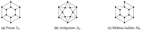
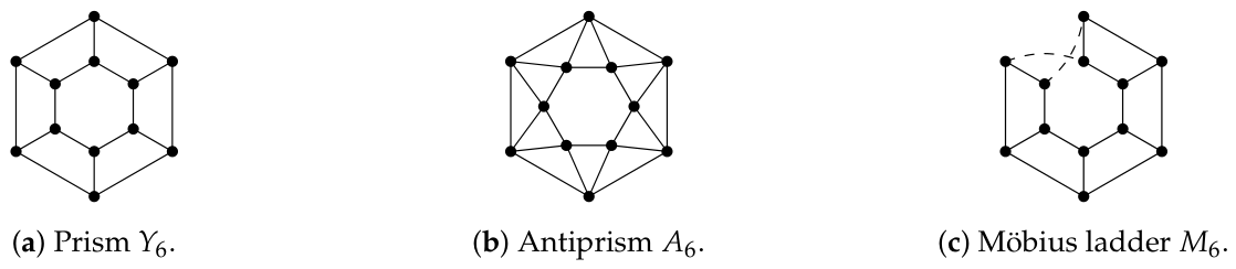
For $n\ge 3$, the antiprism $A_n$ has vertex set $\{u_i,v_i:i\in \mathbb{Z}/n\mathbb{Z}\}$ and edges $u_i{u}_{i+1}$, $v_i{v}_{i+1}$, $u_i{v}_i$, and $u_i{v}_{i+1}$, with all indices read modulo n; see Figure 1. A transfer state is a pair $(a,b)\in {\Omega }_q$, where $a=c\left(u_i\right)$ and $b=c\left(v_i\right)$. A transition $(a,b)\to (a^{\prime },b^{\prime })$ is admissible precisely when $a^{\prime }\ne a$, $b^{\prime }\ne b$, $b^{\prime }\ne a$, and $a^{\prime }\ne b^{\prime }$. To count admissible successors: $b^{\prime }$ must avoid $\{a,b\}$, giving $q-2$ choices; for each such $b^{\prime }$ (with $b^{\prime }\ne a$ already enforced), $a^{\prime }$ must avoid $\{a,b^{\prime }\}$, giving another $q-2$ choices. Hence, every state has exactly ${(q-2)}^2$ admissible successors, and the constant-sector eigenvalue is ${\lambda }_0\left(q\right)={(q-2)}^2$.

Figure 1. Three graph families: prism $Y_6$, antiprism $A_6$, and Möbius ladder $M_6$ (each on 12 vertices; here $M_n$ denotes the n-layer twisted ladder).

The induced action on the row–column sector is given by

$$A_q^A=\left(\begin{array}{cc}-(q-3)& -(q-2)\\ 1& -(q-2)\end{array}\right).$$

(2)

To verify this, let $F(a,b)=g\left(a\right)+h\left(b\right)$ with ${\sum }_{i}g\left(i\right)={\sum }_{i}h\left(i\right)=0$. Summing $g\left(a^{\prime }\right)+h\left(b^{\prime }\right)$ over admissible successors, and using $\sum g=\sum h=0$ to evaluate the resulting partial sums, one obtains $\left(T_q^{A}F\right)(a,b)=-(q-3)g\left(a\right)-(q-2)h\left(a\right)+g\left(b\right)-(q-2)h\left(b\right)$. The coefficient pair $(g,h)$ is therefore mapped to $(-(q-3)g-(q-2)h,g-(q-2\left)h\right)$, which is the action of $A_q^A$ on the two-dimensional coefficient factor. The characteristic polynomial is ${\lambda }^2-(5-2q)\lambda +{(q-2)}^2$, the discriminant is $\Delta \left(q\right)=9-4q$, and the spectral branches are ${\lambda }_{\pm }\left(q\right)=\left(5-2q\pm \sqrt{9-4q}\right)/2$.

Because $A_n$ does not satisfy the J-reversal condition $T_{q}f=-Jf$ on ${\mathcal{U}}_q$, its residual sector requires a direct computation from the transition rule.

Proposition 4

(Antiprism residual action). For every $f\in {\mathcal{U}}_q$ and every $(a,b)\in {\Omega }_q$, one has $\left(T_q^{A}f\right)(a,b)=f(a,b)$. Consequently, $T_q^A{|}_{{\mathcal{U}}_q}=+\mathrm{Id}$, and the residual sector contributes eigenvalue $+1$ with multiplicity $q^2-3q+1$.

Proof. 

Fix $(a,b)\in {\Omega }_q$. The admissible successors are those $(a^{\prime },b^{\prime })\in {\Omega }_q$ satisfying $a^{\prime }\ne a$, $b^{\prime }\ne b$, and $b^{\prime }\ne a$. Apply inclusion–exclusion to these three forbidden conditions starting from ${\sum }_{(a^{\prime },b^{\prime })\in {\Omega }_q}f(a^{\prime },b^{\prime })$. Since $f\in {\mathcal{U}}_q$, every row sum and every column sum of f vanishes by Remark 1; in particular the full sum, the row sum at $a^{\prime }=a$, and the column sums at $b^{\prime }=b$ and $b^{\prime }=a$ all equal zero. Among the pairwise intersections: $\{a^{\prime }=a\}\cap \{b^{\prime }=b\}$ contributes the single term $f(a,b)$ (valid since $a\ne b$); $\{a^{\prime }=a\}\cap \{b^{\prime }=a\}$ is empty in ${\Omega }_q$ because it forces $a^{\prime }=b^{\prime }$; and $\{b^{\prime }=b\}\cap \{b^{\prime }=a\}$ is empty because it forces $a=b$. The triple intersection is empty. Inclusion–exclusion therefore gives $\left(T_q^{A}f\right)(a,b)=0-0-0-0+f(a,b)+0+0-0=f(a,b)$. Since $(a,b)$ was arbitrary, $T_q^A$ fixes ${\mathcal{U}}_q$ pointwise. The multiplicity is $\dim {\mathcal{U}}_q=q(q-1)-1-2(q-1)=q^2-3q+1$. □

Together, the preceding computation and the row–column reduction give $\mathrm{tr}\left({\left(T_q^A\right)}^n\right)={(q-2)}^{2n}+(q-1)\mathrm{tr}\left({\left(A_q^A\right)}^n\right)+(q^2-3q+1)$, from which the branch expansion follows immediately.

Theorem 3

(Branch expansion of $A_n$). For all $z\in \mathbb{C}$ and all $n\ge 3$,

$$P(A_n,z)={(z-2)}^{2n}+(z-1){\lambda }_{+}{\left(z\right)}^n+(z-1){\lambda }_{-}{\left(z\right)}^n+(z^2-3z+1),$$

(3)

where ${\lambda }_{\pm }\left(z\right)=\left(5-2z\pm \sqrt{9-4z}\right)/2$.

Proof. 

For integers $q\ge 3$, Proposition 1 gives $P(A_n,q)=\mathrm{tr}\left({\left(T_q^A\right)}^n\right)$. The constant sector contributes ${(q-2)}^{2n}$. The row–column sector contributes $(q-1)\mathrm{tr}\left({\left(A_q^A\right)}^n\right)=(q-1)({\lambda }_{+}{\left(q\right)}^n+{\lambda }_{-}{\left(q\right)}^n)$. Proposition 4 gives the residual contribution $q^2-3q+1$. Summing yields (3) for all integers $q\ge 3$. The power sum $S_n={\lambda }_{+}^n+{\lambda }_{-}^n$ satisfies the Newton recurrence $S_n=(5-2z)S_{n-1}-{(z-2)}^2{S}_{n-2}$ with $S_0=2$ and $S_1=5-2z$, both polynomial in z, so $S_n$ is polynomial in z for each fixed n. Both sides of (3) are therefore polynomial in z and agree for infinitely many integer values, hence, they are identical for all $z\in \mathbb{C}$. □

Verification at $n=3$. One has ${\lambda }_{\pm }\left(3\right)=(-1\pm i\sqrt{3})/2=e^{\pm 2\pi i/3}$, so ${\lambda }_{\pm }{\left(3\right)}^3=1$. Substituting into (3) gives $P(A_3,3)=1^6+(3-1)(1+1)+(9-9+1)=6$. The graph $A_3$ is the octahedral graph, equivalently the complete tripartite graph $K_{2,2,2}$ [15]. Its proper 3-colorings assign one color class to each antipodal pair, and hence, there are $3!=6$ such colorings. This confirms $P(A_3,3)=P(K_{2,2,2},3)=6$.

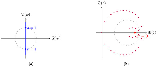
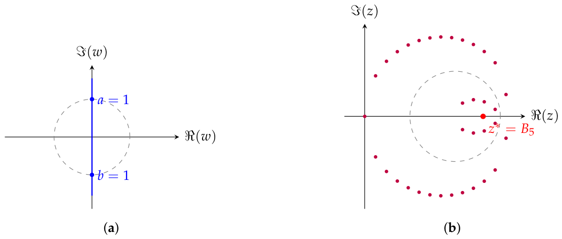
Setting $w=\sqrt{9-4z}$, so that $w^2=9-4z$ and $5-2z=(1+w^2)/2$, the spectral branches factor as ${\lambda }_{\pm }\left(z\right)={(w\pm 1)}^2/4$. The product formula ${\lambda }_{+}\left(z\right){\lambda }_{-}\left(z\right)={(w^2-1)}^2/16$ simplifies via $w^2-1=8-4z=4(2-z)$ to ${\lambda }_{+}\left(z\right){\lambda }_{-}\left(z\right)={(z-2)}^2={\lambda }_0\left(z\right)$. Writing $a= |{\lambda }_{+}\left(z\right)|$ and $b= |{\lambda }_{-}\left(z\right)|$, the four branch moduli are ${\lambda }_0:{|z-2|}^2=ab$; ${\lambda }_{+}:a$; ${\lambda }_{-}:b$; residual: 1. No two of the four branches ${\lambda }_0,{\lambda }_{+},{\lambda }_{-},1$ differ by a unimodular constant: each pairwise ratio equals one of ${\lambda }_{+},{\lambda }_{-},{\lambda }_{+}/{\lambda }_{-},{\lambda }_0$ or a reciprocal thereof, and none of these is constant on an open set, so the hypotheses of Theorem 2 hold. Their pairwise equimodular boundaries are $a=1$, $b=1$, $ab=1$, and $a=b$. The boundary $ab=1$, i.e., $|z-2|=1$, is a circle in the z-plane; the boundary $a=b$ reduces to $\mathrm{Re}\left(w\right)=0$, a half-line on the real axis $x\ge 9/4$. The candidate equimodular locus governed by the Beraha–Kahane–Weiss theorem is therefore contained in the union of the quartic arising from $a=1$ and $b=1$ (competition between the row–column branches and the constant residual branch of modulus 1) together with this circle and half-line; the actual accumulation set is the subset on which the relevant pair of branches is dominant, determined rigorously in Proposition 5 and illustrated in Figure 2.

Figure 2. (a) the two unit-modulus circles $a=1$, $b=1$ in the w-plane (schematic). (b) the equimodular locus of $A_n$, plotted as computed solution points of $Q(x,y)=0$ from (4); the dashed circle $|z-2|=1$ separates the outer arc (where ${\lambda }_0$ and one row–column branch dominate) from the inner arc (where a row–column branch and the residual 1 dominate), and the red point is the isolated accumulation point $z^{\ast }=B_5$ of Theorem 5. (a) Unit-modulus circles in the w-plane (schematic); (b) computed points of $Q(x,y)=0$ with the circle $|z-2|=1$.

Theorem 4

(Quartic equimodular curve). Fix a determination of $w=\sqrt{9-4z}$ on a simply connected domain avoiding the ray $\{z\in \mathbb{R}:9-4z\ge 0\}$, and label the branches by ${\lambda }_{\pm }\left(z\right)={(w\pm 1)}^2/4$. For this determination, the two loci $\{z\in \mathbb{C}:|{\lambda }_{+}\left(z\right)|=1\}$ and $\{z\in \mathbb{C}:|{\lambda }_{-}\left(z\right)|=1\}$ are in general distinct: for example, with $w\left(0\right)=3$ one has ${\lambda }_{+}\left(0\right)=4$ and ${\lambda }_{-}\left(0\right)=1$, so $z=0$ lies on the second locus but not the first. Their union is the real quartic curve $Q(x,y)=0$, where $z=x+iy$ and

$$Q(x,y):=x^4-8x^3+2x^2{y}^2+21x^2-8x{y}^2-18x+y^4+5y^2.$$

(4)

This union is independent of the chosen determination, since replacing w by $-w$ interchanges ${\lambda }_{+}$ and ${\lambda }_{-}$. Moreover, Q is irreducible over $\mathbb{Q}[x,y]$.

Proof. 

Let $z=x+iy$ and choose a square root $w=u+iv$ satisfying $w^2=9-4z$. Equating real and imaginary parts of $w^2=9-4z$ gives $u^2-v^2=9-4x$ and $uv=-2y$.

Since ${\lambda }_{\pm }\left(z\right)={\displaystyle \frac{{(w\pm 1)}^2}{4}}$, the condition $|{\lambda }_{+}\left(z\right)|=1$ is equivalent to $|w+1|=2$. Expanding yields ${(u+1)}^2+v^2=4$, or equivalently $u^2+v^2+2u=3$. Combining this relation with $u^2-v^2=9-4x$ gives $u^2+u=6-2x$ and $v^2=2x-3-u$.

Squaring the identity $uv=-2y$ yields $u^2{v}^2=4y^2$. Substituting $u^2=6-2x-u$ and $v^2=2x-3-u$ gives $(6-2x-u)(2x-3-u)=4y^2$. After expansion and a second substitution of $u^2=6-2x-u$, the equation simplifies to $(6-2x)(2x-2)-4u=4y^2$, and hence, $u=(x-1)(3-x)-y^2$.

Substituting this expression for u into $u^2+u=6-2x$ and simplifying yields precisely the quartic equation $Q(x,y)=0$. Therefore, every point satisfying $|{\lambda }_{+}\left(z\right)|=1$ lies on the quartic $Q(x,y)=0$.

For the branch ${\lambda }_{-}$, the condition $|{\lambda }_{-}\left(z\right)|=1$ is equivalent to $|w-1|=2$, or $u^2+v^2-2u=3$. The resulting system differs from the preceding one only by replacing u with $-u$. The same elimination therefore produces the identical quartic polynomial $Q(x,y)$. Consequently, every point satisfying $|{\lambda }_{-}\left(z\right)|=1$ also lies on $Q(x,y)=0$. Combining the two forward inclusions, every point of $\{|{\lambda }_{+}\left(z\right)|=1\}\cup \{|{\lambda }_{-}\left(z\right)|=1\}$ satisfies $Q(x,y)=0$.

It remains to prove the converse and verify that the elimination process introduces no extraneous points. Assume that $Q(x,y)=0$ and define $u=(x-1)(3-x)-y^2$. Direct substitution into Q shows that $u^2+u=6-2x$. Now define $v^2:=2x-3-u$. Then, $u^2-v^2=u^2-(2x-3-u)=u^2+u-2x+3=9-4x$.

Moreover, $u^2{v}^2=u^2(2x-3-u)$. Using $u^2=6-2x-u$ gives $u^2{v}^2=(6-2x-u)(2x-3-u)=4y^2$, and therefore, ${\left(uv\right)}^2=4y^2$.

To show that v is real, first suppose that $u\ne 0$. Then, $v^2=4y^2/u^2\ge 0$. If $u=0$, the identity $u^2+u=6-2x$ forces $x=3$. Substituting $x=3$ into $u=(x-1)(3-x)-y^2$ gives $y=0$, and consequently, $v^2=2x-3-u=3>0$. Hence, $v^2\ge 0$ in all cases, so a real value of v exists. Choose its sign so that $uv=-2y$.

Setting $w=u+iv$, we obtain $w^2=(u^2-v^2)+2iuv=(9-4x)-4iy=9-4z$. Thus, w is indeed a square root of $9-4z$.

Next, ${|w+1|}^2={(u+1)}^2+v^2=u^2+v^2+2u+1$. Using $u^2+u=6-2x$ and $v^2=2x-3-u$ yields ${|w+1|}^2=(6-2x)+(2x-3)+1=4$, so $|w+1|=2$. If the fixed determination of $\sqrt{9-4z}$ equals this w, then $|{\lambda }_{+}\left(z\right)|=\left|{(w+1)}^2/4\right|=1$; if it equals $-w$, then $|{\lambda }_{-}\left(z\right)|=\left|{(-w-1)}^2/4\right|={|w+1|}^2/4=1$. In either case, the point z lies in the union $\{|{\lambda }_{+}\left(z\right)|=1\}\cup \{|{\lambda }_{-}\left(z\right)|=1\}$.

We conclude that $\{z\in \mathbb{C}:|{\lambda }_{+}\left(z\right)|=1\}\cup \{z\in \mathbb{C}:|{\lambda }_{-}\left(z\right)|=1\}=\{(x,y)\in {\mathbb{R}}^2:Q(x,y)=0\},$ and, since interchanging w and $-w$ merely swaps the two sets in the union, this locus is independent of the chosen determination of $\sqrt{9-4z}$.

For irreducibility, write $Q=y^4+A\left(x\right)y^2+B\left(x\right)$, where $A\left(x\right)=2x^2-8x+5$ and $B\left(x\right)=x(x-2){(x-3)}^2$.

Since Q is primitive as a polynomial in y, Gauss’s lemma reduces the problem to irreducibility over the field $F=\mathbb{Q}\left(x\right)$. The polynomial $B\left(x\right)$ is not a square in F because the factors x and $x-2$ occur with odd multiplicity. Furthermore, $A{\left(x\right)}^2-4B\left(x\right)=25-8x$, which is not a square in F since it has a simple zero at $x=25/8$.

Assume, for contradiction, that Q is reducible over F. If Q possessed a linear factor, then it would have a root $y_0\in F$. Consequently, $y_0^2$ would be a root of $t^2+A\left(x\right)t+B\left(x\right)$, forcing $y_0^2=\left(-A\left(x\right)\pm \sqrt{A{\left(x\right)}^2-4B\left(x\right)}\right)/2$. This would imply $\sqrt{25-8x}\in F$, contrary to the preceding observation. Therefore, Q has no linear factor over F.

Any nontrivial factorization must therefore be quadratic. Since the coefficient of $y^3$ vanishes, such a factorization has the form $Q=(y^2+py+r)(y^2-py+s),$ with $p,r,s\in F$. Comparing coefficients gives $p(s-r)=0$, $r+s-p^2=A$, and $rs=B$.

If $p=0$, then r and s are roots of $t^2-A\left(x\right)t+B\left(x\right)$. Its discriminant is $A{\left(x\right)}^2-4B\left(x\right)=25-8x$, which is not a square in F, a contradiction.

If $s=r$, then $r^2=B\left(x\right)$, which would make $B\left(x\right)$ a square in F, again a contradiction.

Both possibilities are impossible. Hence, no quadratic factorization exists, and Q is irreducible over $F=\mathbb{Q}\left(x\right)$. Gauss’s lemma then implies that Q is irreducible over $\mathbb{Q}[x,y]$. □

Setting $y=0$ gives $Q(x,0)=x(x-2){(x-3)}^2$, so the quartic meets the real axis at $x=0$, $x=2$, and $x=3$; the double factor at $x=3$ marks a singular point of the curve. Indeed, $Q_x(3,0)=Q_y(3,0)=0$, while $Q_{xx}(3,0)=6$, $Q_{yy}(3,0)=-2$, $Q_{xy}(3,0)=0$ give Hessian determinant $6·(-2)-0=-12<0$, so $(3,0)$ is a node at which two real branches cross, not a smooth tangency. In Beraha notation $B_k=4{\cos }^2(\pi /k)$, these real intersections are $B_2=0$, $B_4=2$, and $B_6=3$.

The next proposition determines which points of $Q(x,y)=0$ actually carry accumulation of chromatic roots, rather than leaving this to the figure.

Proposition 5

(Dominant arcs on the antiprism quartic). Write ${\mu }_0={(z-2)}^2$, ${\mu }_1={\lambda }_{+}\left(z\right)$, ${\mu }_2={\lambda }_{-}\left(z\right)$, and ${\mu }_3=1$ for the four branches of (3), so that ${\mu }_1{\mu }_2={\mu }_0$. On the component of $Q(x,y)=0$ where $|{\mu }_1| =1$ one has $|{\mu }_2| = |{\mu }_0{| =|z-2|}^2$, and on the component where $|{\mu }_2| =1$ one has $|{\mu }_1| = |{\mu }_0{| =|z-2|}^2$. Consequently, away from the node $z=3$, exactly two branches attain the maximum modulus, the ratio of these two dominant branches equals ${\lambda }_{+}\left(z\right)$ or ${\lambda }_{-}\left(z\right)$ and is nonconstant, and the corresponding amplitudes in (3) are nonzero; at $z=3$ all four branches have modulus 1. Hence, the entire curve $Q(x,y)=0$ is the equimodular accumulation locus of $\left\{A_n\right\}$. The circle $|z-2|=1$ meets $Q(x,y)=0$ only at the node $z=3$ and separates it into an outer arc $|z-2|>1$, on which ${\mu }_0$ and the modulus-${|z-2|}^2$ row–column branch dominate, and an inner arc $|z-2|<1$, on which the unit-modulus row–column branch and the residual ${\mu }_3=1$ dominate.

Proof. 

The identity ${\mu }_1{\mu }_2={\mu }_0$ is ${\lambda }_{+}{\lambda }_{-}={(z-2)}^2$. On $|{\mu }_1| =1$, it gives $|{\mu }_2| = |{\mu }_0|/|{\mu }_1| = |{\mu }_0{| =|z-2|}^2$; the case $|{\mu }_2| =1$ is symmetric. At such a point, the four moduli are ${|z-2|}^2,1,{|z-2|}^2,1$, so the maximum equals $\max (|z-2{|}^2,1)$. On $Q(x,y)=0$, the equation $|z-2|=1$ forces $z=3$: writing $y^2=1-{(x-2)}^2$ and substituting into Q gives $Q=2(x-3)$, whereas $x=3$ and $y=0$. Away from $z=3$ one has $|z-2|\ne 1$, so the maximum is attained by exactly two branches. If $|z-2|>1$ the dominant pair is $\{{\mu }_0,{\mu }_2\}$ on the first component (respectively $\{{\mu }_0,{\mu }_1\}$ on the second), with ratio ${\mu }_0/{\mu }_2={\mu }_1={\lambda }_{+}$ (respectively ${\mu }_0/{\mu }_1={\mu }_2={\lambda }_{-}$); if $|z-2|<1$ the dominant pair is $\{{\mu }_1,{\mu }_3\}$ (respectively $\{{\mu }_2,{\mu }_3\}$), with ratio ${\mu }_1/{\mu }_3={\lambda }_{+}$ (respectively ${\lambda }_{-}$). At the node $z=3$, all four moduli equal 1; among the tied branches, the pair $\{{\mu }_1,{\mu }_3\}$ has nonconstant ratio ${\lambda }_{+}$ and nonzero amplitudes $z-1=2$ and $z^2-3z+1=1$, so this multiple-tie point also accumulates. In every case the ratio of two dominant branches is a nonconstant analytic function. The amplitudes 1, $z-1$, and $z^2-3z+1$ appearing in (3) do not vanish on $Q(x,y)=0$: their zeros $z=1$ and $z=(3\pm \sqrt{5})/2$ give $Q(1,0)=-4$, $Q((3-\sqrt{5})/2,0)=-(2+\sqrt{5})$, and $Q((3+\sqrt{5})/2,0)=\sqrt{5}-2$, all nonzero. Applying Theorem 2 on each analytic branch domain, as in the remark following it, identifies every point of $Q(x,y)=0$ as an accumulation point of zeros of $\left\{P(A_n,z)\right\}$, with the two dominance types separated by the node $z=3$. □

Theorem 5

(Isolated accumulation point). The antiprism family has an isolated accumulation point at $z^{\ast }=(3+\sqrt{5})/2={\varphi }^2=B_5$. This is the unique zero of the residual amplitude ${\alpha }_1\left(z\right)=z^2-3z+1$ lying in the open region where the constant residual branch is uniquely dominant.

Proof. 

Set $z^{\ast }=(3+\sqrt{5})/2$. Then, $9-4z^{\ast }=3-2\sqrt{5}<0$, so $\sqrt{9-4z^{\ast }}=is$ with $s=\sqrt{2\sqrt{5}-3}>0$, and $|{\lambda }_{\pm }\left(z^{\ast }\right)| = |{(1\pm is)}^2|/4=(1+s^2)/4$. Substituting $s^2=2\sqrt{5}-3$ gives $1+s^2=2\sqrt{5}-2$, hence, $|{\lambda }_{\pm }\left(z^{\ast }\right)| =(\sqrt{5}-1)/2<1$. Also, $|{\lambda }_0\left(z^{\ast }\right)| ={(z^{\ast }-2)}^2={((\sqrt{5}-1)/2)}^2=(3-\sqrt{5})/2<1$. Since all three non-residual branches have modulus less than 1 at $z^{\ast }$ and the constant residual has modulus 1, the residual is uniquely dominant at $z^{\ast }$ and remains so throughout a neighborhood U of $z^{\ast }$.

The residual amplitude is ${\alpha }_1\left(z\right)=z^2-3z+1$. Its roots are $(3\pm \sqrt{5})/2$, so ${\alpha }_1\left(z^{\ast }\right)=0$ and ${\alpha }_1\not\equiv 0$. Proposition 3 therefore implies that $z^{\ast }$ is an isolated limit point of chromatic roots of $\left\{A_n\right\}$.

The other root $z^{\ast \ast }=(3-\sqrt{5})/2$ satisfies $|{\lambda }_0\left(z^{\ast \ast }\right)|={(z^{\ast \ast }-2)}^2={(1+\sqrt{5})}^2/4={\varphi }^2>1$, so ${\lambda }_0$ is dominant at $z^{\ast \ast }$ and the residual branch is not. Hence, $z^{\ast }$ is the only zero of ${\alpha }_1$ in the region where the residual is uniquely dominant. □

Proposition 6.

$z^{\ast }=(3+\sqrt{5})/2=4{\cos }^2(\pi /5)={\varphi }^2=B_5$.

Proof. 

The identity $\cos (\pi /5)=(1+\sqrt{5})/4$ gives $4{\cos }^2(\pi /5)={(1+\sqrt{5})}^2/4=(3+\sqrt{5})/2$. Since $\varphi =(1+\sqrt{5})/2$, one has ${\varphi }^2=(3+\sqrt{5})/2$. Hence, $z^{\ast }=4{\cos }^2(\pi /5)={\varphi }^2=B_5$. □

4. Spectral Deformations: Möbius, Circulant, and Chord

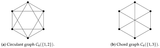
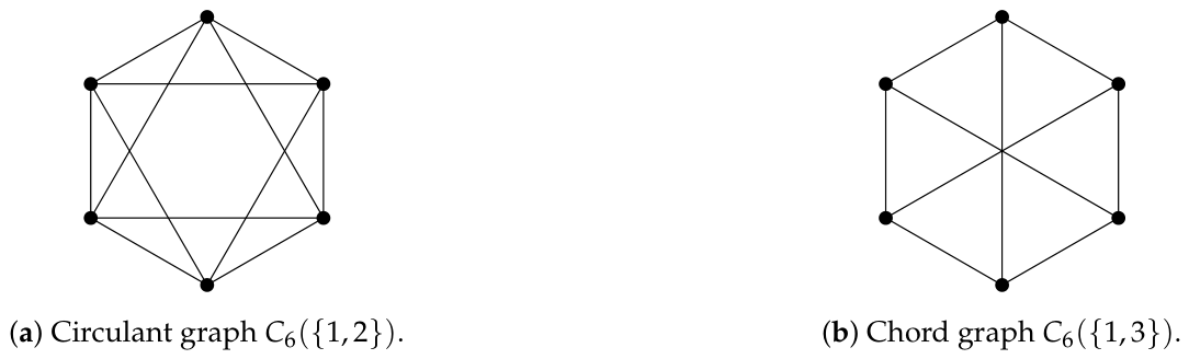
The antiprism’s accumulation geometry is driven by the discriminant $\Delta \left(z\right)=9-4z$ of its reduced transfer matrix and the flat residual eigenvalue $+1$. The three families studied here each arise from a closely related construction and deviate from the antiprism in one precisely controlled way: the Möbius ladder preserves the prism spectrum but alters the amplitudes through a twisted closure; the circulant $C_n\left(\{1,2\}\right)$ (see, for e.g., Figure 3a) independently reproduces the discriminant $9-4z$; and the chord family $C_n\left(\{1,3\}\right)$ (see, for e.g., Figure 3b) satisfies a product identity on its reduced branches that forces the quartic geometry to degenerate to a segment. The contrast among these cases shows that the equimodular geometry is determined by the discriminant and determinant of the reduced transfer matrix, not by the graph structure alone.

Figure 3. Circulant graphs defined by jump sets $\{1,2\}$ and $\{1,3\}$, illustrated for $n=6$. Panel (b) shows the jump structure only; the chord analysis of Section 4.3 assumes $n\ge 7$, for which the two distance-3 neighbors are distinct.

4.1. The Möbius Ladder

The Möbius ladder $M_n$, shown in Figure 1c, is obtained from the prism $Y_n$ by a twisted cyclic closure: the terminal interface $(u_n,v_n)$ is identified with $(v_1,u_1)$ rather than $(u_1,v_1)$. A proper q-coloring of $M_n$ corresponds to a state sequence $s_0,s_1,\dots ,s_{n-1}$ in which each transition $s_i\to s_{i+1}$ is admissible and the closing condition is $s_n=J\left(s_0\right)$ rather than $s_n=s_0$, where J is the transposition involution $\left(Jf\right)(a,b)=f(b,a)$. The number of such twisted closed walks is $\mathrm{tr}\left(T_q^{n}J\right)$, giving the twisted trace formula $P(M_n,q)=\mathrm{tr}\left(T_q^{n}J\right)$.

Since the local transition rule for $M_n$ is identical to that of the prism $Y_n$, the transfer matrix and its eigenvalues are unchanged. By [12], the prism transfer operator has four spectral branches ${\lambda }_0=q^2-3q+3$, ${\lambda }_1=3-q$, ${\lambda }_2=1-q$, and ${\lambda }_3=1$, with corresponding eigenspaces: the constant space $\mathbb{C}\mathbf{1}$ for ${\lambda }_0$; the J-symmetric subspace of ${\mathcal{W}}_q$ for ${\lambda }_1$; the J-antisymmetric subspace of ${\mathcal{W}}_q$ for ${\lambda }_2$; and ${\mathcal{U}}_q$ for ${\lambda }_3$. The computation of $\mathrm{tr}\left(T_q^{n}J\right)$ proceeds sector by sector. Writing $P_j$ for the spectral projector onto the eigenspace of ${\lambda }_j$:

The constant sector: $J\mathbf{1}=\mathbf{1}$, so $\mathrm{tr}\left(P_{0}J\right)={\mathbf{1}}^{T}J\mathbf{1}/|{\Omega }_q|=1$, contributing ${(q^2-3q+3)}^n$.

The row–column sector: on the J-symmetric eigenspace of ${\lambda }_1$, J acts as the identity, so $\mathrm{tr}\left(P_{1}J\right)=q-1$, contributing $(q-1){(3-q)}^n$. On the J-antisymmetric eigenspace of ${\lambda }_2$, J acts as $-\mathrm{Id}$, so $\mathrm{tr}\left(P_{2}J\right)=-(q-1)$, contributing $-(q-1){(1-q)}^n$.

The residual sector: since J has no fixed point on ${\Omega }_q$ (a fixed point would require $a=b$), $\mathrm{tr}\left(J\right)=0$. The four sector contributions must sum to zero: $\mathrm{tr}\left(P_{\mathrm{res}}J\right)=\mathrm{tr}\left(J\right)-\mathrm{tr}\left(P_{0}J\right)-\mathrm{tr}\left(P_{1}J\right)-\mathrm{tr}\left(P_{2}J\right)=0-1-(q-1)+(q-1)=-1,$ contributing $1^n·(-1)=-1$.

Summing gives

$$P(M_n,z)={(z^2-3z+3)}^n+(z-1){(3-z)}^n-(z-1){(1-z)}^n-1.$$

(5)

Both sides are polynomial in z and agree for all integers $q\ge 3$, so the identity holds for all $z\in \mathbb{C}$. Since the twisted closure modifies amplitudes but not eigenvalues, $M_n$ shares its pairwise equimodular loci with the prism family.

4.2. The Circulant $C_n\left(\{1,2\}\right)$ and the Shared Discriminant

For $n\ge 5$, let $X_n=C_n\left(\{1,2\}\right)$ have vertex set $\mathbb{Z}/n\mathbb{Z}$ with edges $i\sim i\pm 1$ and $i\sim i\pm 2$. The bound $n\ge 5$ ensures the graph is simple: when $n=4$, the vertex $i+2\equiv i-2\left(\mathrm{mod}4\right)$ collapses two distance-2 neighbors to one, giving $C_4\left(\{1,2\}\right)=K_4$, while for $n=5$ all adjacencies are distinct and $C_5\left(\{1,2\}\right)=K_5$.

The transfer construction records two consecutive colors as a state $(a,b)\in {\Omega }_q$. A transition $(a,b)\to (b,c)$ is admissible when $c\notin \{a,b\}$, enforcing both the distance-1 constraint $c\ne b$ and the distance-2 constraint $c\ne a$. For fixed $(a,b)$, there are exactly $q-2$ admissible choices for c, giving constant-sector eigenvalue ${\lambda }_0\left(q\right)=q-2$.

To derive the row–column action, let $F(a,b)=g\left(a\right)+h\left(b\right)$ with ${\sum }_{i}g\left(i\right)={\sum }_{i}h\left(i\right)=0$. Then, $\left(T_q^{X}F\right)(a,b)={\sum }_{c\notin \{a,b\}}(g\left(b\right)+h\left(c\right))=(q-2)g\left(b\right)+{\sum }_{c\notin \{a,b\}}h\left(c\right).$ Since ${\sum }_{c}h\left(c\right)=0$ and $a\ne b$, one has ${\sum }_{c\notin \{a,b\}}h\left(c\right)=-h\left(a\right)-h\left(b\right)$, and thus, $\left(T_q^{X}F\right)(a,b)=-h\left(a\right)+(q-2)g\left(b\right)-h\left(b\right).$ The coefficient pair $(g,h)$ maps to $(-h,(q-2)g-h)$, so the reduced action on the row–column sector is $A_q^X=\left(\begin{array}{cc}0& -1\\ q-2& -1\end{array}\right),$ with characteristic polynomial ${\lambda }^2+\lambda +(q-2)$ and discriminant $\Delta \left(q\right)=1-4(q-2)=9-4q$. The reduced spectral branches are therefore ${\lambda }_{\pm }\left(z\right)=(-1\pm \sqrt{9-4z})/2$.

For the residual sector, let $f\in {\mathcal{U}}_q$. Then, $\left(T_q^{X}f\right)(a,b)={\sum }_{c\notin \{a,b\}}f(b,c)={\sum }_{c\ne b}f(b,c)-f(b,a),$ and ${\sum }_{c\ne b}f(b,c)=0$ by the zero row-sum condition of Remark 1. Hence, $\left(T_q^{X}f\right)(a,b)=-f(b,a)=-\left(Jf\right)(a,b)$, so $T_q^X{|}_{{\mathcal{U}}_q}=-J$. Proposition 2 therefore applies, and the residual sector contributes eigenvalue $-1$ with multiplicity $q(q-3)/2$ and eigenvalue $+1$ with multiplicity $(q-1)(q-2)/2$. The two residual branches $+1$ and $-1$ differ by the unimodular constant $-1$; the hypothesis of Theorem 2 therefore excludes this pair from producing an accumulation curve, consistent with their common modulus being constant. Among the remaining pairs, every ratio is one of ${\lambda }_0/{\lambda }_{\pm }$, ${\lambda }_{+}/{\lambda }_{-}$, ${\lambda }_{\pm }/(\pm 1)$, or ${\lambda }_0/(\pm 1)$, none constant on an open set, so apart from the excluded pair $\{+1,-1\}$, the hypotheses of Theorem 2 are met.

Theorem 6

(Branch expansion of $C_n\left(\{1,2\}\right)$). For all $z\in \mathbb{C}$ and all $n\ge 5$,

$$P(C_n\left(\{1,2\}\right),z)={(z-2)}^n+(z-1){\lambda }_{+}{\left(z\right)}^n+(z-1){\lambda }_{-}{\left(z\right)}^n+{\displaystyle \frac{z(z-3)}{2}}{(-1)}^n+{\displaystyle \frac{(z-1)(z-2)}{2}},$$

(6)

where ${\lambda }_{\pm }\left(z\right)=(-1\pm \sqrt{9-4z})/2$. For $n=5$, this reduces to $P(K_5,z)=z(z-1)(z-2)(z-3)(z-4)$.

Proof. 

For integer $q\ge 3$, the trace formula gives $P(C_n\left(\{1,2\}\right),q)=\mathrm{tr}\left({\left(T_q^X\right)}^n\right)$. The constant sector contributes ${(q-2)}^n$. Since the row–column action is $A_q^X\otimes I_{q-1}$, the row–column sector contributes $(q-1)({\lambda }_{+}{\left(q\right)}^n+{\lambda }_{-}{\left(q\right)}^n)$. By Proposition 2, the residual sector contributes ${\displaystyle \frac{q(q-3)}{2}}{(-1)}^n+{\displaystyle \frac{(q-1)(q-2)}{2}}$. Summing yields (6) for all integers $q\ge 3$. The power sum ${\lambda }_{+}^n+{\lambda }_{-}^n$ is polynomial in q by the Newton recurrence with initial values $S_0=2$ and $S_1=-1$ and step $S_k=-S_{k-1}-(q-2)S_{k-2}$; all other terms in (6) are visibly polynomial. Hence, both sides are polynomial in q, and the polynomial identity extends the formula to all $z\in \mathbb{C}$.

For $n=5$, $C_5\left(\{1,2\}\right)=K_5$. Evaluating the right side of (6) at $z=0,1,2,3,4$ gives 0 in each case (verified from the recurrence with $\det A_q^X=q-2$), so the formula yields a monic degree-five polynomial with roots $0,1,2,3,4$, confirming $P(C_5\left(\{1,2\}\right),z)=P(K_5,z)$. □

Setting $w=\sqrt{9-4z}$, the circulant branches are ${\lambda }_{\pm }\left(z\right)=(-1\pm w)/2$. The equimodular conditions $|{\lambda }_{\pm }\left(z\right)|=1$ become $|-1\pm w|=2$, i.e., $|w\mp 1|=2$, which are exactly the same two circles in the w-plane that arise in the antiprism analysis (Theorem 4), with branch labels interchanged. Their pullback under $w^2=9-4z$ is again the quartic $Q(x,y)=0$ from (4). The shared discriminant $9-4z$ is thus the precise spectral reason for the identical limiting geometry, even though the two families differ substantially as graphs.

Corollary 1

(Shared w-plane modulus locus implies shared equimodular geometry). Let $\left\{G_n\right\}$ and $\left\{H_n\right\}$ be closed recursively layered graph families whose reduced $2\times 2$ transfer matrices have spectral branches ${\lambda }_{\pm }^G$, ${\lambda }_{\pm }^H$ and a common linear discriminant $\Delta \left(z\right)$. Fix $w=\sqrt{\Delta \left(z\right)}$, so $w^2=\Delta \left(z\right)$, and suppose that under this substitution the conditions $\{|{\lambda }_{+}^G|=1\}$, $\{|{\lambda }_{-}^G|=1\}$ and the conditions $\{|{\lambda }_{+}^H|=1\}$, $\{|{\lambda }_{-}^H|=1\}$ determine the same unordered pair of curves $\mathcal{C}$ in the w-plane. Then, the reduced unit-modulus loci coincide,

$$\{z\in \mathbb{C}:|{\lambda }_{+}^G|=1\}\cup \{z:|{\lambda }_{-}^G|=1\}=\{z\in \mathbb{C}:|{\lambda }_{+}^H|=1\}\cup \{z:|{\lambda }_{-}^H|=1\},$$

and equal the preimage of $\mathcal{C}$ under the covering $w^2=\Delta \left(z\right)$.

In particular, for the antiprism $A_n$ and the circulant $C_n\left(\{1,2\}\right)$ the common discriminant is $\Delta \left(z\right)=9-4z$ and the common w-plane locus is the pair of circles $|w+1|=2$, $|w-1|=2$; its pullback under $w^2=9-4z$ is the irreducible quartic $Q(x,y)=0$ of Theorem 4. This holds even though the trace and determinant of the two reduced matrices differ.

Proof. 

Because $\Delta$ is linear with a nonzero leading coefficient, $w^2=\Delta \left(z\right)$ defines a single-valued map $\pi :w\mapsto z={\Delta }^{-1}\left(w^2\right)$. For a $2\times 2$ reduced operator, each condition $|{\lambda }_{\pm }\left(z\right)|=1$ pulls back under $w^2=\Delta \left(z\right)$ to a condition on w alone; by hypothesis, the union of the two conditions is, for both families, the same curve set $\mathcal{C}$. Hence,

$$\{z:|{\lambda }_{+}^G|=1\}\cup \{z:|{\lambda }_{-}^G|=1\}=\pi \left(\mathcal{C}\right)=\{z:|{\lambda }_{+}^H|=1\}\cup \{z:|{\lambda }_{-}^H|=1\}.$$

For the two named families, ${\lambda }_{\pm }^A={(w\pm 1)}^2/4$ gives $|{\lambda }_{+}^A| =1\iff |w+1|=2$ and $|{\lambda }_{-}^A| =1\iff |w-1|=2$, while ${\lambda }_{\pm }^X=(-1\pm w)/2$ gives $|{\lambda }_{+}^X| =1\iff |w-1|=2$ and $|{\lambda }_{-}^X| =1\iff |w+1|=2$. Both produce the unordered pair $\mathcal{C}=\{|w-1|=2,|w+1|=2\}$, whose pullback under $w^2=9-4z$ was computed in Theorem 4 to be $Q(x,y)=0$. □

Because the two residual branches $+1$ and $-1$ differ by the constant unimodular factor $-1$, Theorem 2 cannot be applied to them as independent branches; the residual sector must first be combined after fixing the parity of n, as recorded by the following elementary lemma.

Lemma 1

(Parity reduction for residual branches $+1$ and $-1$). Let $P_n\left(z\right)={\sum }_{j=1}^r{a}_j\left(z\right){\lambda }_j{\left(z\right)}^n+{\alpha }_{-}\left(z\right){(-1)}^n+{\alpha }_{+}\left(z\right)$. For $ϵ\in \{0,1\}$, write $n=2m+ϵ$. Then,

$$P_{2m+ϵ}\left(z\right)={\displaystyle \sum _{j=1}^r}{a}_j\left(z\right){\lambda }_j{\left(z\right)}^{ϵ}{\left({\lambda }_j{\left(z\right)}^2\right)}^m+{\beta }_{ϵ}\left(z\right),$$

(7)

where ${\beta }_0\left(z\right)={\alpha }_{+}\left(z\right)+{\alpha }_{-}\left(z\right)$ and ${\beta }_1\left(z\right)={\alpha }_{+}\left(z\right)-{\alpha }_{-}\left(z\right)$. The set of limit points of zeros of $\left\{P_n\right\}$ is the union of the sets of limit points of the two parity subsequences $\left\{P_{2m}\right\}$ and $\left\{P_{2m+1}\right\}$.

Proof. 

Substituting $n=2m+ϵ$ gives ${\lambda }_j^n={\lambda }_j^{ϵ}{\left({\lambda }_j^2\right)}^m$ and ${(-1)}^n={(-1)}^{ϵ}$, which yields (7) and the two amplitudes. If $z_0$ is a limit point of zeros of $\left\{P_n\right\}$, there are $n_k\to \infty$ and zeros $z_k\to z_0$; one parity occurs for infinitely many $n_k$, so $z_0$ is a limit point of that parity subsequence. The converse is immediate, since each parity subsequence is a subsequence of $\left\{P_n\right\}$. □

For $X_n=C_n\left(\{1,2\}\right)$, the amplitudes are ${\alpha }_{-}\left(z\right)=z(z-3)/2$ and ${\alpha }_{+}\left(z\right)=(z-1)(z-2)/2$, so ${\beta }_0\left(z\right)=z^2-3z+1$ for even n and ${\beta }_1\left(z\right)=1$ for odd n. The even residual amplitude therefore has the same zeros as the antiprism residual amplitude, and this produces an isolated accumulation point along the even subsequence.

Proposition 7

(Even-subsequence isolated point for $C_n\left(\{1,2\}\right)$). Let $X_n=C_n\left(\{1,2\}\right)$ and $z^{\ast }=(3+\sqrt{5})/2=B_5$. Then, $z^{\ast }$ is an isolated accumulation point of chromatic roots of the even subsequence $\left\{P(X_{2m},z)\right\}$, hence, of the full family $\left\{P(X_n,z)\right\}$; the odd subsequence has no isolated point from residual amplitude cancellation.

Proof. 

By Lemma 1 the even subsequence has residual branch 1 with amplitude ${\beta }_0\left(z\right)=z^2-3z+1$, and ${\beta }_0\left(z^{\ast }\right)=0$. At $z^{\ast }$, $9-4z^{\ast }=3-2\sqrt{5}<0$, so $\sqrt{9-4z^{\ast }}=is$ with $s=\sqrt{2\sqrt{5}-3}$, and $|{\lambda }_{\pm }\left(z^{\ast }\right){|}^2=(1+s^2)/4=(\sqrt{5}-1)/2<1$; also, $|z^{\ast }{-2|}^2={((\sqrt{5}-1)/2)}^2=(3-\sqrt{5})/2<1$. In the squared-branch system $\{{(z-2)}^2,{\lambda }_{+}^2,{\lambda }_{-}^2,1\}$ of (7), the residual branch 1 is therefore uniquely dominant at $z^{\ast }$, and remains so throughout a neighborhood. Since ${\beta }_0\not\equiv 0$, Proposition 3 gives an isolated accumulation point at $z^{\ast }$. The other zero $z^{\ast \ast }=(3-\sqrt{5})/2$ is excluded because $|z^{\ast \ast }-2|=(1+\sqrt{5})/2>1$, so ${(z-2)}^2$ dominates there. For odd n, the residual amplitude is ${\beta }_1\equiv 1$, which has no zeros, so no residual isolated point arises. □

Away from the isolated point, the whole quartic accumulates for each parity, exactly as for the antiprism.

Proposition 8

(Dominance on the circulant quartic). Let ${\lambda }_0\left(z\right)=z-2$ and ${\lambda }_{\pm }\left(z\right)=(-1\pm \sqrt{9-4z})/2$, so that ${\lambda }_{+}{\lambda }_{-}=z-2={\lambda }_0$ by Vieta. On $Q(x,y)=0$, if $|{\lambda }_i| =1$ for one row–column branch and ${\lambda }_j$ denotes the other, then $|{\lambda }_j| = |{\lambda }_0| =|z-2|$, and the four moduli are $|z-2|,1,|z-2|,1$. The circle $|z-2|=1$ meets $Q(x,y)=0$ only at $z=3$. Away from $z=3$, the dominant pair is $\{{\lambda }_0,{\lambda }_j\}$ when $|z-2|>1$ and $\{{\lambda }_i,1\}$ when $|z-2|<1$; at $z=3$ all relevant branches have modulus 1. Applying Theorem 2 after the parity split of Lemma 1, whose squared branches carry the nonconstant ratios ${\lambda }_i^2$, the entire quartic $Q(x,y)=0$ is the equimodular accumulation locus of each parity subsequence of $\left\{X_n\right\}$.

Proof. 

The product identity is Vieta’s formula for ${\lambda }^2+\lambda +(z-2)$. On $|{\lambda }_i| =1$, the relation $|{\lambda }_i{\lambda }_j| =|z-2|$ gives $|{\lambda }_j| =|z-2|= |{\lambda }_0|$, so the four moduli are $|z-2|,1,|z-2|,1$. The circulant equimodular locus is the same quartic $Q(x,y)=0$ (Corollary 1), and on it, $|z-2|=1$ forces $z=3$ by the substitution $y^2=1-{(x-2)}^2$, which gives $Q=2(x-3)$. If $|z-2|>1$, the branches ${\lambda }_0,{\lambda }_j$ dominate; after the parity split, their squares have equal modulus and ratio ${({\lambda }_0/{\lambda }_j)}^2={\lambda }_i^2$, which is nonconstant. If $|z-2|<1$, the branches ${\lambda }_i,1$ dominate, with squared ratio ${\lambda }_i^2$, again nonconstant. At $z=3$, all branches tie, and at least one admissible dominant-pair ratio is nonconstant. The relevant amplitudes do not vanish on $Q(x,y)=0$: $z-1\ne 0$ there, the even residual amplitude $z^2-3z+1$ has zeros $(3\pm \sqrt{5})/2\notin Q$, and the odd residual amplitude is 1. Hence, Theorem 2 gives accumulation along the entire quartic for both parities. □

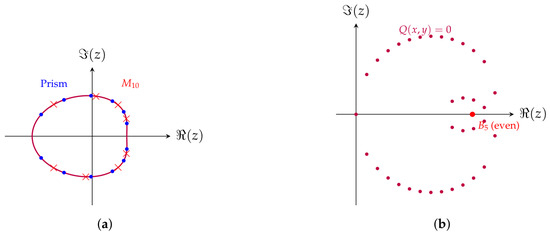
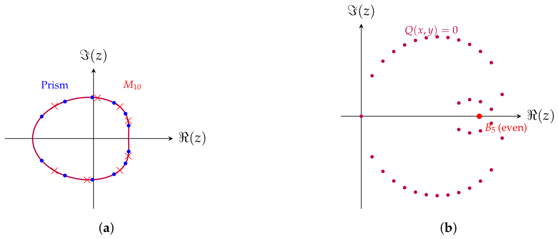
The two parity subsequences of $M_n$ and $C_n\left(\{1,2\}\right)$ are shown in Figure 4.

Figure 4. (a) prism and Möbius ladder $M_{10}$, governed by the prism equimodular curve from ${\lambda }_0=z^2-3z+3$ (distinct from Q); this panel is schematic. (b) the shared quartic (4) governing $C_n\left(\{1,2\}\right)$, plotted as computed solution points of $Q(x,y)=0$; the red point is the even-subsequence isolated accumulation point $B_5$ of Proposition 7. (a) Prism and Möbius ladder roots (schematic); (b) $C_n\left(\{1,2\}\right)$: computed $Q(x,y)=0$ and even-subseq. point $B_5$.

4.3. The Chord Graph $C_n\left(\{1,3\}\right)$ and a Degenerate Equimodular Locus

For $n\ge 7$, let $C_n\left(\{1,3\}\right)$ have vertex set $\mathbb{Z}/n\mathbb{Z}$ and edges $i\sim i\pm 1$ and $i\sim i\pm 3$. The bound $n\ge 7$ ensures the two distance-3 neighbors $i\pm 3$ are distinct: for $n=6$, one has $i+3\equiv i-3\left(\mathrm{mod}6\right)$, so the jump-3 edges form a perfect matching and the local transition counts below change; the analysis assumes the generic case $n\ge 7$. The distance-3 edges couple vertices three steps apart, so the transfer construction must retain three consecutive colors. A transfer state has the form $(a,b,c)$ with $a\ne b$ and $b\ne c$, representing the color triple $(x_{i-2},x_{i-1},x_i)$. Appending $d=x_{i+1}$ requires $d\ne c$ (the distance-1 edge $i\sim i+1$) and $d\ne a$ (the distance-3 edge $(i-2)\sim (i+1)$); no distance-2 constraint arises since $i-1$ and $i+1$ are not adjacent in $C_n\left(\{1,3\}\right)$.

Under the $S_q$-orbit decomposition, the state space $\left\{\right(a,b,c):a\ne b,b\ne c\}$ has two orbit types: Type I, where $a=c$ (count $q(q-1)$), and Type II, where $a\ne c$ (count $q(q-1)(q-2)$). For an $S_q$-invariant function f that takes value x on Type I and y on Type II:

On a Type I state $(a,b,a)$: d avoids only $\left\{a\right\}$, giving $q-1$ successors. Exactly one has $d=b$ (type Type I successor $(b,a,b)$) and $q-2$ have $d\notin \{a,b\}$ (Type II successors). Hence, $\left(T_q^{C}f\right)(a,b,a)=x+(q-2)y.$

On a Type II state $(a,b,c)$ with $a\ne c$: d avoids $\{a,c\}$, giving $q-2$ successors. Exactly one has $d=b$ (the Type I successor $(b,c,b)$) and $q-3$ have $d\notin \{a,b,c\}$ (Type II successors). Hence, $\left(T_q^{C}f\right)(a,b,c)=x+(q-3)y.$

The reduced action on the two-dimensional orbit-type sector is therefore represented by $B_q^C=\left(\begin{array}{cc}1& q-2\\ 1& q-3\end{array}\right)$, with characteristic polynomial $(\lambda -1)(\lambda -(q-3))-(q-2)={\lambda }^2-(q-2)\lambda -1$, giving the reduced spectral branches ${\lambda }_{\pm }\left(z\right)=\left((z-2)\pm \sqrt{z^2-4z+8}\right)/2$ and the product ${\lambda }_{+}\left(z\right){\lambda }_{-}\left(z\right)=-1$ (Vieta).

Theorem 7

(Equimodular locus of the reduced spectral pair for $C_n\left(\{1,3\}\right)$). The reduced branches satisfy ${\lambda }_{+}\left(z\right){\lambda }_{-}\left(z\right)=-1$, and the equimodular locus of the pair $\{{\lambda }_{+},{\lambda }_{-}\}$ is exactly ${\mathcal{E}}_C=\{z\in \mathbb{C}:\mathrm{Re}z=2,|\mathrm{Im}z|\le 2\}$.

Proof. 

The product identity is immediate from Vieta’s formulas. If $|{\lambda }_{+}\left(z\right)|= |{\lambda }_{-}\left(z\right)|$, then taking moduli gives $|{\lambda }_{+}{\left(z\right)|}^2=|{\lambda }_{+}\left(z\right){\lambda }_{-}\left(z\right)|=1$, so both branches have modulus 1. Choose $\theta \in \mathbb{R}$ with ${\lambda }_{+}\left(z\right)=e^{i\theta }$. Substituting into ${\lambda }^2-(z-2)\lambda -1=0$ and dividing by $e^{i\theta }$ gives $e^{i\theta }-e^{-i\theta }=z-2$, i.e., $2i\sin \theta =z-2$, hence, $z=2+2i\sin \theta$. Thus, $\mathrm{Re}z=2$ and $|\mathrm{Im}z|\le 2$.

Conversely, let $z=2+it$ with $|t|\le 2$ and choose $\theta \in \mathbb{R}$ with $2\sin \theta =t$. Then, $z-2=e^{i\theta }-e^{-i\theta }$, and substituting $\lambda =e^{i\theta }$ into the characteristic equation gives $e^{2i\theta }-(e^{i\theta }-e^{-i\theta })e^{i\theta }-1=e^{2i\theta }-e^{2i\theta }+1-1=0.$ So $e^{i\theta }$ is a root. The second root is $-e^{-i\theta }$ (since the product of the two roots equals $-1$), which also has modulus 1. Hence, $|{\lambda }_{+}\left(z\right)|= |{\lambda }_{-}\left(z\right)|$, completing the characterization. □

We stress that Theorem 7 describes only the reduced $2\times 2$ orbit-type sector $B_q^C$; the full transfer decomposition and the dominance of ${\lambda }_{\pm }$ over the residual sectors are not established here, so the segment is the reduced-pair equimodular locus rather than a proven limiting root set. The product identity ${\lambda }_{+}{\lambda }_{-}=-1$ is the spectral mechanism that collapses the quartic geometry. Whereas the antiprism and circulant families have $|{\lambda }_{+}| =1$ and $|{\lambda }_{-}| =1$ defining distinct circles in the w-plane whose pullbacks produce a quartic, the chord family has $|{\lambda }_{+}| = |{\lambda }_{-}| =1$ simultaneously, and the parametrization $z=2+2i\sin \theta$ traces out a line segment rather than the nondegenerate quartic algebraic curve found in the antiprism and circulant cases. This transition from quartic to segment is the geometric content of level two in the spectral hierarchy of Section 6.

5. The Ladder Graph and the Generalized Petersen Family

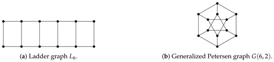
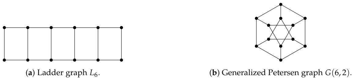
The two families studied here occupy opposite ends of the spectral hierarchy. The ladder graph $L_n$ (Figure 5a) has a single dominant spectral branch, so the Beraha–Kahane–Weiss mechanism produces no equimodular accumulation curve whatsoever. The generalized Petersen graph $G(n,2)$ (Figure 5b) has an irreducible cubic spectral equation, placing its accumulation geometry beyond the quadratic analysis of the preceding sections. Together they delimit the range of behavior stated in Remark 2.

Figure 5. Ladder graph $L_n$ and Generalized Petersen family $G(n,2)$ for $n=6$.

5.1. The Ladder Graph $L_n$

The ladder $L_n=P_n\square P_2$ is the Cartesian product of a path on n vertices with a single edge; it has $2n$ vertices arranged as two parallel paths connected by n rungs. Because the family has open boundary conditions, the transfer formula of Proposition 1 applies in its vector form. A transfer state is a pair $(a,b)\in {\Omega }_q$. A transition $(a,b)\to (a^{\prime },b^{\prime })$ is admissible when $a^{\prime }\ne a$, $b^{\prime }\ne b$, and $a^{\prime }\ne b^{\prime }$. For a fixed state $(a,b)$, there are initially $q(q-1)$ ordered pairs $(a^{\prime },b^{\prime })$ with $a^{\prime }\ne b^{\prime }$; exactly $q-1$ have $a^{\prime }=a$, exactly $q-1$ have $b^{\prime }=b$, and exactly one pair satisfies both conditions (namely $(a,b)$ itself). Inclusion–exclusion gives $q(q-1)-2(q-1)+1=q^2-3q+3$ admissible successors for every state, so $T_q\mathbf{1}=(q^2-3q+3)\mathbf{1}$.

Theorem 8

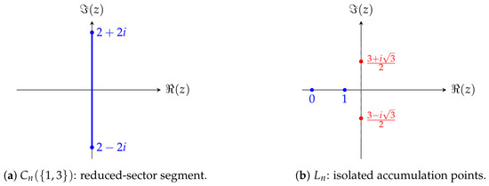
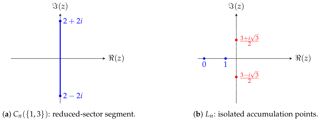
(Chromatic polynomial of $L_n$). For all $n\ge 1$ and all $z\in \mathbb{C}$, $P(L_n,z)=z(z-1){(z^2-3z+3)}^{n-1}$. The full fixed-zero set is $\{0,1,(3+i\sqrt{3})/2,(3-i\sqrt{3})/2\}$; the zeros 0 and 1 occur with fixed multiplicity 1, while $(3\pm i\sqrt{3})/2$ occur with multiplicity $n-1$. After the universal chromatic factors $z(z-1)$ are removed, the only remaining fixed zeros—and the only zeros of unbounded multiplicity—are $(3\pm i\sqrt{3})/2$. Since a single spectral branch survives the open-boundary projection, no equimodular accumulation curve occurs.

Proof. 

The first rung of $L_n$ is an edge and contributes $q(q-1)$ colorings. Since $T_q\mathbf{1}=(q^2-3q+3)\mathbf{1}$, the open-boundary transfer formula with $\mathbf{v}=\mathbf{w}=\mathbf{1}$ gives $P(L_n,q)={\mathbf{1}}^T{T}_q^{n-1}\mathbf{1}={(q^2-3q+3)}^{n-1}{\mathbf{1}}^T\mathbf{1}=q(q-1){(q^2-3q+3)}^{n-1}$ for every integer $q\ge 0$. Both sides are polynomial in q, so the identity holds for all $z\in \mathbb{C}$.

The factorization shows that every zero of $P(L_n,z)$ is either 0, 1, or a root of $z^2-3z+3$. The roots of $z^2-3z+3$ are $(3\pm i\sqrt{3})/2$, and each appears with multiplicity $n-1$ for all $n\ge 2$; they are therefore fixed zeros of the family of unbounded multiplicity, and trivially its only nontrivial limit points. Since the chromatic polynomial involves only the single spectral branch $\lambda \left(z\right)=z^2-3z+3$, no two branches can compete in modulus, and the first condition of Theorem 2 never applies. The sole accumulation mechanism is that of fixed zeros, and no equimodular accumulation curve arises. □

Figure 6 compares the isolated-point behavior of the ladder with the vertical segment arising for $C_n\left(\{1,3\}\right)$.

Figure 6. Degenerate limiting geometries for the chord and ladder families. Both panels are exact: the chord panel shows the reduced-sector segment of Theorem 7; the ladder panel shows the exact fixed zeros of Theorem 8.

5.2. The Generalized Petersen Family $G(n,2)$

For $n\ge 5$, the generalized Petersen graph $G(n,2)$ has vertex set $\{u_i,v_i:i\in \mathbb{Z}/n\mathbb{Z}\}$ with outer cycle edges $u_i{u}_{i+1}$, spokes $u_i{v}_i$, and inner edges $v_i{v}_{i+2}$. Unlike the prism and antiprism families, the inner edges couple vertices separated by two layers, so the transfer process must retain one previous inner color. Accordingly, a transfer state is represented by a triple $(a,b,c)=(c\left(u_i\right),c\left(v_i\right),c\left(v_{i-1}\right)),$ where the spoke constraint forces $a\ne b$.

A transition $(a,b,c)\to (a^{\prime },b^{\prime },b)$ is admissible precisely when the new layer satisfies all adjacency constraints: $a^{\prime }\ne a$ (from the outer edge $u_i{u}_{i+1}$), $a^{\prime }\ne b^{\prime }$ (from the spoke $u_{i+1}{v}_{i+1}$), and $b^{\prime }\ne c$ (from the inner edge $v_{i-1}{v}_{i+1}$). The colour-relabeling group $S_q$ acts on the state set $\left\{\right(a,b,c):a\ne b\}$, and an $S_q$-invariant function depends only on the equality pattern of $(a,b,c)$. Since $a\ne b$ is fixed, there are exactly three patterns, so the invariant sector is 3-dimensional, spanned by the indicators of

$$T_1=\{c=a\},T_2=\{c=b\},T_3=\{a,b,c\mathrm{distinct}\}.$$

Write an invariant f as the triple $(x_1,x_2,x_3)$ of its values on $T_1,T_2,T_3$. The reduced action sends f to the function whose value at a state is $\sum f(a^{\prime },b^{\prime },b)$ over the admissible successors $(a^{\prime },b^{\prime },b)$, those with $a^{\prime }\ne a$, $a^{\prime }\ne b^{\prime }$, and $b^{\prime }\ne c$; a successor lies in $T_1$ when $b=a^{\prime }$, in $T_2$ when $b=b^{\prime }$, and in $T_3$ otherwise. Counting the successors of each pattern gives the following.

From $T_1$ (so $c=a$): the $T_1$ successors ($a^{\prime }=b$) require $b^{\prime }\notin \{a,b\}$, giving $q-2$; the $T_2$ successors ($b^{\prime }=b$) require $a^{\prime }\notin \{a,b\}$, giving $q-2$; the $T_3$ successors require $a^{\prime }\notin \{a,b\}$ then $b^{\prime }\notin \{a,b,a^{\prime }\}$, giving $(q-2)(q-3)$.

From $T_2$ (so $c=b$): the $T_1$ successors ($a^{\prime }=b$) require $b^{\prime }\ne b$, giving $q-1$; no $T_2$ successor exists, since $b^{\prime }=b$ violates $b^{\prime }\ne c=b$; the $T_3$ successors require $a^{\prime }\notin \{a,b\}$ and $b^{\prime }\notin \{a^{\prime },b\}$, giving ${(q-2)}^2$.

From $T_3$ ($a,b,c$ distinct): the $T_1$ successors ($a^{\prime }=b$) require $b^{\prime }\notin \{b,c\}$, giving $q-2$; the $T_2$ successors ($b^{\prime }=b$) require $a^{\prime }\notin \{a,b\}$, giving $q-2$; the $T_3$ successors require $a^{\prime }\notin \{a,b\}$ and $b^{\prime }\notin \{a^{\prime },b,c\}$, which yields $q-2$ choices of $b^{\prime }$ when $a^{\prime }=c$ and $q-3$ otherwise, hence, $(q-2)+{(q-3)}^2=q^2-5q+7$.

Collecting the counts as the matrix whose $(i,j)$-entry is the number of type-$T_j$ successors of a type-$T_i$ state gives

$$B_q=\left(\begin{array}{ccc}q-2& q-2& (q-2)(q-3)\\ q-1& 0& {(q-2)}^2\\ q-2& q-2& q^2-5q+7\end{array}\right).$$

The remaining $S_q$-isotypic sectors contribute lower-dimensional residual blocks that we do not record here.

We can check with the case when $q=3$. Direct enumeration of the admissible single-layer extensions yields the integer matrix $B_3=\left(\begin{array}{ccc}1& 1& 0\\ 2& 0& 1\\ 1& 1& 1\end{array}\right)$, whose characteristic polynomial is ${\lambda }^3-2{\lambda }^2-2\lambda +2$, in agreement with Theorem 9. We emphasize that Theorem 9 establishes the cubic as the spectral equation of this three-dimensional invariant sector; its dominance over the remaining $S_q$-isotypic sectors is not established here, and a complete branch expansion of $P\left(G\right(n,2),z)$, including the residual amplitudes, is not derived. The higher-degree accumulation geometry below is therefore stated as structural evidence and an open direction, not as a proved classification.

Theorem 9

(Cubic spectral equation). The characteristic polynomial of $B_q{|}_{q=z}$ is $f(\lambda ,z)={\lambda }^3-(z^2-4z+5){\lambda }^2-(z^3-5z^2+8z-4)\lambda +(z-1)(z-2),$ and $f(\lambda ,z)$ is irreducible over $\mathbb{Q}\left(z\right)$.

Proof. 

Setting $p=z-2$, a direct expansion of $\det (\lambda I-B_q){|}_{q=z}$ gives ${\lambda }^3-(p^2+1){\lambda }^2-p^2(p+1)\lambda +p(p+1)$. Substituting back: $p^2+1={(z-2)}^2+1=z^2-4z+5$; $p^2(p+1)={(z-2)}^2(z-1)=z^3-5z^2+8z-4$; and $p(p+1)=(z-2)(z-1)=(z-1)(z-2)$. This gives the stated polynomial. One can verify that at $z=3$, we have $f(\lambda ,3)={\lambda }^3-2{\lambda }^2-2\lambda +2$ with a direct expansion from $B_3=\left(\begin{array}{ccc}1& 1& 0\\ 2& 0& 1\\ 1& 1& 1\end{array}\right)$ to confirm the result.

For irreducibility over $\mathbb{Q}\left(z\right)$: since f is monic in $\lambda$ with coefficients in $\mathbb{Q}\left[z\right]$ and $\mathbb{Q}\left[z\right]$ is integrally closed, any root of f in $\mathbb{Q}\left(z\right)$ must lie in $\mathbb{Q}\left[z\right]$. A cubic over a field is reducible if and only if it has a root in that field, so it suffices to show f has no root $p\left(z\right)\in \mathbb{Q}\left[z\right]$. The constant term $(z-1)(z-2)$ forces $p\left(z\right)$ to divide $(z-1)(z-2)$ in $\mathbb{Q}\left[z\right]$, so $p\left(z\right)\in \{c,c(z-1),c(z-2),c(z-1\left)\right(z-2\left)\right\}$ for some $c\in {\mathbb{Q}}^{\times }$.

If $p\left(z\right)=c$: the leading power of z in $f(c,z)$ is $z^3$ with coefficient $-c$, forcing $c=0$, a contradiction.

If $p\left(z\right)=c(z-1)$: the coefficient of $z^4$ in $f\left(p\right(z),z)$ is $-c^2-c$, so $c=-1$. Then, $f(1-z,z)=-(z-1)(z^2-2z+2)$; since $z^2-2z+2={(z-1)}^2+1$ has no real roots and is not identically zero, $f(1-z,z)\not\equiv 0$.

If $p\left(z\right)=c(z-2)$: the $z^4$ coefficient is again $-c^2-c$, giving $c=-1$. Then, $f(2-z,z)=z-2\not\equiv 0$.

If $p\left(z\right)=c(z-1)(z-2)$: the coefficient of $z^6$ in $f\left(p\right(z),z)$ is $c^3-c^2$, giving $c=1$. Then, $f((z-1)(z-2),z)=-(z-1)(z-2)(z^2-3z+1)\not\equiv 0$.

In every case $f\left(p\right(z),z)\not\equiv 0$, so f has no root in $\mathbb{Q}\left(z\right)$ and is therefore irreducible over $\mathbb{Q}\left(z\right)$. □

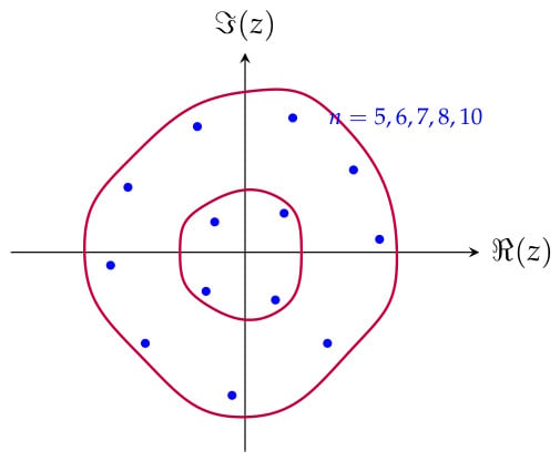
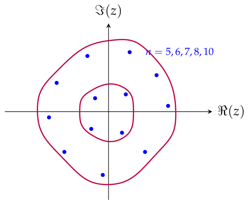
The three spectral branches of $G(n,2)$ are thus algebraic of degree three over $\mathbb{Q}\left(z\right)$. Their equimodular geometry is not governed by a single quadratic discriminant, and the pairwise modulus-competition locus is a higher-degree real algebraic set whose structure lies beyond the methods of the preceding sections. The numerical root distributions in Figure 7 are consistent with multibranch cubic competition but do not constitute a proof of a specific algebraic degree for the accumulation set.

Figure 7. Schematic chromatic-root distribution for $G(n,2)$ ($n=5,6,7,8,10$); curves and points illustrate multibranch cubic competition and are not computed loci. This figure is exploratory only and is not used as evidence for the results of the paper.

6. Spectral Hierarchy and Consequences

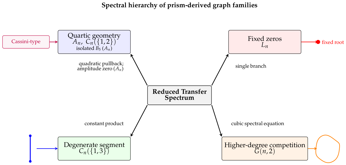
The families studied in the preceding sections are governed by a common spectral mechanism: the limiting chromatic-root geometry is determined not by the graph structure directly, but by the dimension and algebraic properties of the reduced transfer operator—specifically its discriminant, its determinant, and the moduli of its branches relative to the constant residual eigenvalue. The following remark summarizes the four qualitatively distinct outcomes exhibited by the families of this paper.

Remark 2

(Spectral hierarchy). The preceding examples exhibit a structural relationship between the reduced transfer spectrum and the geometry of the limiting chromatic-root locus.

1. 

For $2\times 2$ reduced transfer operators with linear discriminant, the unit-modulus conditions reduce under $w^2=\Delta \left(z\right)$ to circle equations in the w-plane. Their quadratic pullbacks produce quartic equimodular curves, as in the antiprism and circulant families $C_n\left(\{1,2\}\right)$, for which the whole quartic is proved to accumulate; see Theorem 4, Proposition 5, and Corollary 1.

2. 

When ${\lambda }_{+}\left(z\right){\lambda }_{-}\left(z\right)=-1$ identically, the equimodular condition forces both branches onto the unit circle, collapsing the reduced-sector geometry to a real line segment rather than a quartic curve; see Theorem 7.

3. 

For reduced transfer operators of degree at least three with irreducible characteristic polynomial over $\mathbb{Q}\left(z\right)$, the equimodular geometry arises from higher-degree algebraic branch competition and is not governed by the quadratic pullback mechanism; see Theorem 9.

4. 

If the boundary conditions project onto a single dominant spectral branch, then no dominant branch competition occurs, and no equimodular accumulation curve arises; see Theorem 8.

These examples suggest that the algebraic complexity of the reduced transfer spectrum strongly constrains the topology and geometry of the limiting chromatic-root set.

Each level of this hierarchy is realized by one or more families studied above. The antiprism $A_n$ and the circulant $C_n\left(\{1,2\}\right)$ both fall under item 1: they share the discriminant $\Delta \left(z\right)=9-4z$, so the conditions $|{\lambda }_{\pm }\left(z\right)|=1$ produce the same two circles in the w-plane and, upon pullback, the same irreducible quartic $Q(x,y)=0$ from (4), and for both this whole quartic carries accumulation by Propositions 5 and 8 together with Corollary 1. Despite their common quartic locus, the two families differ in the way the residual sector enters the trace. For the antiprism, the residual branch is $+1$ with amplitude $z^2-3z+1$, giving the isolated accumulation point $z^{\ast }=B_5$. For the circulant, the residual branches $+1$ and $-1$ must be combined by parity (Lemma 1): the even subsequence carries the same amplitude $z^2-3z+1$, and hence, the same isolated point $B_5$ (Proposition 7), while the odd subsequence carries the constant amplitude 1 and has no such point. Thus, both the antiprism and the even circulant subsequence exhibit the isolated point $B_5$. The prism $Y_n$ also realizes item 1, but through a different quadratic mechanism: its reduced row–column matrix has the constant discriminant 4, so the relevant quadratic branch is the constant-sector eigenvalue ${\lambda }_0=z^2-3z+3$, whose unit-modulus competition produces a quartic equimodular curve distinct from $Q(x,y)$. The Möbius ladder $M_n$ shares the full prism spectrum, and hence, shares that same prism quartic—again not $Q(x,y)$. Thus, the shared quartic Q of (4) is specific to the pair $\{A_n,C_n\left(\{1,2\}\right)\}$, which alone realize the linear-discriminant pullback $w^2=9-4z$.

The chord family $C_n\left(\{1,3\}\right)$ falls under item 2. Its reduced branches satisfy ${\lambda }_{+}\left(z\right){\lambda }_{-}\left(z\right)=-1$ (Theorem 7), and the unit-circle parametrization ${\lambda }_{+}=e^{i\theta }$ forces $z-2=2i\sin \theta$, collapsing the reduced-sector equimodular locus to the segment ${\mathcal{E}}_C=\{\mathrm{Re}z=2,|\mathrm{Im}z|\le 2\}$. The determinant condition ${\lambda }_{+}{\lambda }_{-}=-1$ is specific to this family; a general unit-determinant condition $|{\lambda }_{+}{\lambda }_{-}| =1$ would yield a one-dimensional equimodular locus, but not necessarily a vertical segment.

The ladder $L_n$ realizes item 4: the open boundary conditions project entirely onto the single branch $\lambda \left(z\right)=z^2-3z+3$, so no branch competition arises and the zeros $(3\pm i\sqrt{3})/2$ are fixed for all $n\ge 2$. The generalized Petersen family $G(n,2)$ realizes item 3: its characteristic polynomial is irreducible of degree three over $\mathbb{Q}\left(z\right)$ (Theorem 9), placing its accumulation geometry beyond the quadratic circle-pullback method.

Table 1 summarizes the spectral profiles, and Figure 8 depicts the hierarchy schematically.

Table 1. Spectral profiles of the prism-derived families.

Family	Degree	Spectral Structure	Limiting Geometry	Isolated Points
Prism $Y_n$	2	const. disc.; ${\lambda }_0=z^2-3z+3$	quartic ‡	none
Antiprism $A_n$	2	$\Delta \left(z\right)=9-4z$	quartic Q	$B_5$
Möbius $M_n$	2	prism spectrum	quartic ‡	none
$C_n\left(\{1,2\}\right)$	2	$\Delta \left(z\right)=9-4z$	quartic Q	$B_5$ along the even subsequence
$C_n\left(\{1,3\}\right)$	2	${\lambda }_{+}{\lambda }_{-}=-1$	segment †, $\mathfrak{R}z=2$	none established
Ladder $L_n$	1	single branch	fixed zeros	fixed nontrivial pair
$G(n,2)$	3	irreducible cubic	higher-degree set	unknown

^† Established as the equimodular locus of the reduced $2\times 2$ spectral pair (Theorem 7); dominance over the residual sectors of the full transfer operator is not analyzed. ^‡ The prism and Möbius equimodular curve is determined by the quadratic constant-sector branch ${\lambda }_0=z^2-3z+3$, the reduced row–column discriminant being the constant 4; it is a quartic in $(\mathrm{Re}z,\mathrm{Im}z)$ distinct from $Q(x,y)$ of (4), obtained in [12]. The shared quartic Q of item 1 in Remark 2 applies only to the pair $\{A_n,C_n\left(\{1,2\}\right)\}$; for that pair, the entire quartic is proved to accumulate by Proposition 5 for $A_n$ and by Proposition 8 for $C_n\left(\{1,2\}\right)$.

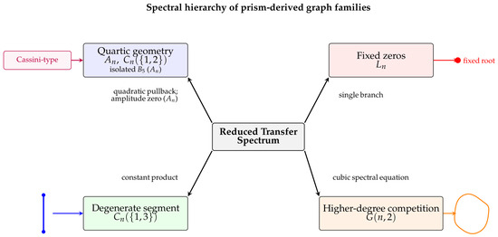
Figure 8. Spectral hierarchy for prism-derived graph families.

The chromatic polynomial arises as the zero-temperature antiferromagnetic specialization of the Potts partition function [3,5], and in the thermodynamic limit, the dominant transfer branch determines the free energy while the equimodular set marks the complex phase boundary [4,8]. Under this correspondence, the quartic (4) is the complex phase boundary for both the antiprism and circulant families; the segment $\{\mathrm{Re}z=2,|\mathrm{Im}z|\le 2\}$ constitutes the equimodular locus of the reduced spectral pair and is therefore the component of the phase boundary of the chord family arising from reduced-sector competition; contributions from the full transfer operator, including any residual sector, are not characterized here.

Several problems remain open. A structural classification of circulant families $C_n\left(S\right)$ whose reduced discriminant equals $9-4q$ would clarify the combinatorial origin of the shared quartic geometry. Whether higher Beraha numbers $B_k$ arise as isolated accumulation points in other prism-derived families through amplitude cancellation within a uniquely dominant residual region remains unresolved. The irreducibility of the cubic spectral equation for $G(n,2)$ suggests the existence of higher-degree equimodular sets, but the algebraic structure of the corresponding accumulation set, together with the missing residual-sector analysis and a full branch expansion, is not yet understood. More broadly, a general theory relating the degree and splitting field of the reduced characteristic polynomial to the topology of the limiting root set would unify the hierarchy of the present paper.

References

- Birkhoff, G.D. A determinant formula for the number of ways of coloring a map. Ann. Math. 1912, 14, 42–46. [Google Scholar] [CrossRef] [Scilit]
- Whitney, H. The coloring of graphs. Ann. Math. 1932, 33, 688–718. [Google Scholar] [CrossRef] [Scilit]
- Fortuin, C.M.; Kasteleyn, P.W. On the random-cluster model I. Introduction and relation to other models. Physica 1972, 57, 536–564. [Google Scholar] [CrossRef] [Scilit]
- Welsh, D.J.A.; Merino, C. The Potts model and the Tutte polynomial. J. Math. Phys. 2000, 41, 1127–1152. [Google Scholar] [CrossRef] [Scilit]
- Potts, R.B. Some generalized order-disorder transformations. Proc. Camb. Philos. Soc. 1952, 48, 106–109. [Google Scholar] [CrossRef] [Scilit]
- Colbourn, C.J. The Combinatorics of Network Reliability; Oxford University Press: Oxford, UK, 1987. [Google Scholar]
- Beraha, S.; Kahane, J.; Weiss, N.J. Limits of zeros of recursively defined families of polynomials. In Studies in Foundations and Combinatorics, Advances in Mathematics, Supplementary Studies; Academic Press: Cambridge, MA, USA, 1978; Volume 1, pp. 213–232. [Google Scholar]
- Salas, J.; Sokal, A.D. Transfer matrices and partition-function zeros for antiferromagnetic Potts models. I. General theory and square-lattice chromatic polynomial. J. Stat. Phys. 2001, 104, 609–699. [Google Scholar] [CrossRef] [Scilit]
- Shrock, R.; Tsai, S.-H. Asymptotic limits and zeros of chromatic polynomials and ground-state entropy of Potts antiferromagnets. Phys. Rev. E 1997, 55, 5165–5178. [Google Scholar] [CrossRef] [Scilit]
- Jackson, B. A zero-free interval for chromatic polynomials of graphs. Comb. Probab. Comput. 1993, 2, 325–336. [Google Scholar] [CrossRef] [Scilit]
- Thomassen, C. The zero-free intervals for chromatic polynomials of graphs. Comb. Probab. Comput. 1997, 6, 497–506. [Google Scholar] [CrossRef] [Scilit]
- Allagan, J.; Voloshin, V.; Deriglazov, V.; Lopez-Bonilla, R.N. Explicit equimodular curves for prism-graph chromatic polynomials and the Beraha–Kahane–Weiss limit set. Amer. J. Comput. Math. 2026, 16, 14–26. [Google Scholar] [CrossRef]
- Allagan, J.; Voloshin, V.; Gao, W.; Deriglazov, V. Chromatic roots of prism graphs: Cassini geometry and a uniform finite-n bound. J. Comb. Math. Comb. Comput. 2026; to appear.
- Lopez-Bonilla, R.N.; Allagan, J.; Langley, S.M.; Clinton, A.J. Chromatic polynomials of graphs. J. Adv. Math. Comput. Sci. 2025, 40, 79–98. [Google Scholar] [CrossRef] [Scilit]
- Biggs, N. Algebraic Graph Theory, 2nd ed.; Cambridge University Press: Cambridge, UK, 1993. [Google Scholar]
Disclaimer/Publisher’s Note: The statements, opinions and data contained in all publications are solely those of the individual author(s) and contributor(s) and not of MDPI and/or the editor(s). MDPI and/or the editor(s) disclaim responsibility for any injury to people or property resulting from any ideas, methods, instructions or products referred to in the content. |
© 2026 by the authors. Licensee MDPI, Basel, Switzerland. This article is an open access article distributed under the terms and conditions of the Creative Commons Attribution (CC BY) license.