A Fuzzy Difference Equation Framework for Water-Consumption Modeling Under Data Uncertainty

Abstract

This paper develops a fuzzy difference equation model for analyzing long-term domestic water-consumption dynamics under parameter uncertainty. The proposed framework combines a difference equation with fuzzy parameter representations, allowing uncertainty to be incorporated directly into the modeling process through triangular fuzzy numbers and their associated $\alpha$-cut intervals. Fundamental properties of the model are investigated, including the existence, boundedness, and nesting behavior of fuzzy solutions. The model is applied to annual domestic water-consumption data from Taiwan covering the period 2008–2024. Parameter estimates are obtained using ordinary least squares, and both deterministic and fuzzy solution trajectories are constructed. Numerical results show that the deterministic model captures the overall long-term behavior of the consumption series, while the fuzzy formulation provides uncertainty bands that contain 94.12% of the observed data. The results demonstrate that the proposed approach offers an interpretable framework for studying water-consumption dynamics while explicitly accounting for uncertainty in model parameters.

1. Introduction

Reliable forecasting and analysis of water consumption play an important role in water-resources planning, infrastructure management, and long-term sustainability studies. Understanding consumption patterns can support decision-making related to resource allocation, capacity expansion, and policy development. A variety of approaches have been proposed for modeling water-consumption dynamics. Early studies focused primarily on statistical and regression-based techniques. For example, Maidment and Miaou [1] examined daily water-use patterns in several cities and highlighted the importance of temporal variability in consumption records. Jain and Ormsbee [2] reviewed short-term forecasting methods and discussed the strengths of regression-based approaches for operational water-demand prediction. Herrera et al. [3] later investigated predictive models for hourly urban water demand and demonstrated that data-driven techniques can successfully capture short-term fluctuations in consumption.

As larger datasets became available, researchers began exploring more sophisticated forecasting frameworks. House-Peters and Chang [4] provided a comprehensive review of urban water-demand modeling and emphasized the influence of demographic, climatic, and socioeconomic factors on consumption patterns. Donkor et al. [5] surveyed forecasting methodologies and concluded that the most appropriate modeling approach often depends on the characteristics of the available data and the intended application. Romano and Kapelan [6] proposed adaptive forecasting strategies for smart water-distribution systems, while Adamowski et al. [7] compared statistical and machine learning techniques and reported that nonlinear methods can provide improved forecasting performance under certain conditions. More recent studies by Oyebode and Ighravwe [8], Pacchin et al. [9], Niknam et al. [10], and Ghannam and Hussain [11] have continued to evaluate forecasting tools and compare the effectiveness of conventional and data-driven approaches.

Although these studies have significantly advanced water-demand forecasting, most of them focus primarily on predictive accuracy and short-term forecasting performance. In contrast, the objective of the present work is to develop a mathematically tractable framework for studying long-term water-consumption dynamics while explicitly accounting for uncertainty. Rather than introducing another forecasting algorithm, we employ a fuzzy difference equation model that allows uncertainty to be incorporated directly into the governing dynamics and analyzed through the evolution of fuzzy solution trajectories.

Despite the success of these approaches, uncertainty remains an inherent feature of water-consumption systems. Population growth, socioeconomic changes, climate variability, measurement errors, and incomplete information can all influence consumption patterns and affect the reliability of model predictions. Consequently, there has been increasing interest in mathematical frameworks capable of representing uncertainty explicitly rather than treating all model parameters as precise quantities.

Fuzzy set theory, introduced by Zadeh [12], provides a natural framework for modeling uncertainty when precise probabilistic information is unavailable. Since its introduction, fuzzy theory has been applied extensively in engineering, environmental sciences, decision-making, and resource management [13,14,15,16,17,18]. Within this framework, uncertain quantities are represented by fuzzy numbers, allowing uncertainty to be incorporated directly into mathematical models while preserving interpretability.

The study of fuzzy dynamical systems has attracted significant attention over the last several decades. Kaleva [19] established foundational results for fuzzy differential equations and demonstrated how uncertainty can be incorporated directly into dynamical models. Puri and Ralescu [20] introduced the concept of fuzzy random variables, providing an alternative framework for representing uncertain quantities. Buckley and Feuring [21] further developed the theory of fuzzy differential equations and investigated practical solution procedures for fuzzy dynamical systems.

Subsequent developments expanded the mathematical foundations of the field. Bede and Gal [22] studied generalized differentiability concepts for fuzzy-valued functions, while Stefanini and Bede [23] extended these ideas to interval-valued systems and generalized Hukuhara differentiability. Together, these contributions have provided important tools for analyzing uncertainty propagation and the qualitative behavior of fuzzy dynamical systems.

Comprehensive treatments of fuzzy mathematics and fuzzy dynamical systems can be found in the works of Dubois and Prade [13], Zimmermann [14], Ross [15], and Bede [24]. Building upon this theoretical foundation, the present study focuses on the application of fuzzy dynamical ideas to long-term water-consumption modeling and investigates how parameter uncertainty influences the evolution of the resulting solution trajectories.

Recent research has continued to expand the role of uncertainty quantification in dynamical systems and environmental applications. In addition to classical fuzzy differential and difference equation models, researchers have investigated interval-valued systems, generalized differentiability concepts, fuzzy random variables, and hybrid uncertainty frameworks that combine fuzzy and numerical approaches [20,21,22]. These developments have broadened the applicability of fuzzy dynamical systems and provided new tools for analyzing uncertainty propagation, stability, and long-term system behavior.

Within water-resources research, fuzzy methodologies have been applied to a variety of practical problems, including rainfall–runoff prediction, groundwater-level forecasting, water-level estimation, and hydrological decision support [25,26,27,28]. Fuzzy neural networks, soft-computing techniques, and uncertainty-aware modeling approaches have demonstrated their usefulness in situations where observations are incomplete or affected by significant uncertainty. These studies highlight the continuing relevance of fuzzy methodologies in water-related applications and motivate the development of interpretable mathematical models that explicitly describe the evolution of uncertainty over time.

Although fuzzy methods have been widely used in hydrology and water-resources management, relatively few studies have focused on fuzzy difference equation models for long-term water-consumption dynamics while simultaneously investigating the mathematical properties of the resulting fuzzy solutions. Much of the existing literature emphasizes predictive performance through machine learning models, fuzzy inference systems, or hybrid soft-computing frameworks. Comparatively less attention has been devoted to developing mathematically tractable fuzzy dynamical models that describe how uncertainty propagates through time and how the structure of fuzzy solutions evolves under the governing dynamics.

The present study aims to address this gap by developing a fuzzy difference equation model for domestic water consumption. Uncertainty is incorporated directly into the model parameters through triangular fuzzy numbers, and the resulting fuzzy solutions are analyzed using an $\alpha$-cut representation. In addition to the numerical investigation, several theoretical properties of the model are established, including existence, boundedness, interval nesting, and symmetry-preservation properties. These results provide insight into both the mathematical structure of the model and its ability to represent uncertainty in long-term consumption dynamics.

To illustrate the proposed framework, annual domestic water-consumption data obtained from the Taiwan Government Open Data Platform [29] are used in the numerical study. The objective is not short-term operational forecasting but rather the analysis of long-term consumption behavior under uncertainty. The proposed framework combines fuzzy uncertainty representation with dynamical-system analysis and provides a foundation for future extensions involving additional explanatory variables, alternative fuzzy structures, and more complex water-consumption systems.

2. Preliminaries

In this section, we briefly review the basic concepts of fuzzy numbers and fuzzy difference equations that will be used throughout the paper. The presentation is kept concise and focused on the elements needed for the proposed model.

2.1. Fuzzy Numbers

A fuzzy number provides a convenient way to represent uncertainty when precise numerical values are not available.

Definition 1.

A fuzzy number $\tilde{A}$ is a function $\tilde{A}:\mathbb{R}\to [0, 1]$ that is normal, convex, upper semi-continuous, and has compact support.

In practice, fuzzy numbers are often described using their $\alpha$-cuts, which provide an interval representation at different confidence levels.

Definition 2.

For $\alpha \in (0, 1]$, the α-cut of a fuzzy number $\tilde{A}$ is defined by

$${\left[\tilde{A}\right]}^{\alpha }=\{x\in \mathbb{R}:\tilde{A}\left(x\right)\ge \alpha \}.$$

Each α-cut is a closed interval that can be written as

$${\left[\tilde{A}\right]}^{\alpha }=[A_L\left(\alpha \right),A_U\left(\alpha \right)].$$

This representation allows us to work with fuzzy numbers through interval arithmetic, which is particularly useful in dynamical systems.

2.2. Fuzzy Difference Equations

Let $\left\{{\tilde{x}}_n\right\}$ be a sequence of fuzzy numbers. A fuzzy difference equation has the general form

$${\tilde{x}}_{n+1}=F(n,{\tilde{x}}_n),$$

where F is a suitable mapping.

Using $\alpha$-cuts, the fuzzy difference equation can be transformed into a family of interval-valued difference equations:

$${\left[x_{n+1}\right]}^{\alpha }=F^{\alpha }(n,{\left[x_n\right]}^{\alpha }),\alpha \in (0, 1].$$

This approach allows the analysis of fuzzy systems by studying the corresponding interval systems.

Remark 1.

In this work, we adopt the α-cut approach, which provides a practical and mathematically consistent way to analyze fuzzy dynamical systems.

3. Model Formulation

3.1. Modeling Assumptions and Motivation

The objective of this study is to analyze the long-term evolution of domestic water consumption under uncertainty through a fuzzy difference equation framework. Using annual per-capita water-consumption observations, the proposed model combines a mean-reverting structure with periodic forcing to describe long-term consumption behavior while accounting for uncertainty in the model parameters. The focus is on understanding long-term consumption patterns and uncertainty propagation rather than short-term forecasting.

Two characteristics are commonly observed in long-term water-consumption records. First, consumption tends to fluctuate around a characteristic long-term level rather than increasing indefinitely. Second, recurring seasonal or cyclical effects often influence consumption patterns through climatic, social, and economic factors. These observations motivate the use of a mean-reverting structure combined with periodic forcing.

Let $D_n$ denote the observed water consumption at year n. The first observation in the dataset is used as the initial condition $D_0$. This initial value serves only as the starting point of the dynamical system and does not represent additional forecasting information.

3.2. Deterministic Difference Equation Model

Based on the above considerations, we consider the deterministic model

$$D_{n+1}=D_n+\kappa (\theta -D_n)+{\gamma }_{1}sin\left({\displaystyle \frac{2\pi n}{T}}\right)+{\gamma }_{2}cos\left({\displaystyle \frac{2\pi n}{T}}\right),$$

where

• $D_n$ denotes water consumption at time n;
• $\theta$ represents the long-term equilibrium consumption level;
• $\kappa$ is the adjustment rate toward equilibrium;
• ${\gamma }_1$ and ${\gamma }_2$ describe periodic fluctuations;
• T denotes the period of the seasonal cycle.

The parameter $\kappa$ controls the speed at which deviations from equilibrium are corrected. When $0<\kappa <1$, consumption gradually returns toward the equilibrium level $\theta$, producing a mean-reverting behavior commonly observed in long-term resource-consumption data.

3.3. Fuzzification of Model Parameters

The parameters obtained from the deterministic model are subject to uncertainty arising from measurement errors, data aggregation, and model simplifications. To account for this uncertainty, the deterministic parameters are extended to fuzzy numbers.

Specifically, the parameters

$$\kappa ,\theta ,{\gamma }_1,{\gamma }_2$$

are replaced by the fuzzy quantities

$$\tilde{\kappa },\tilde{\theta },{\tilde{\gamma }}_1,{\tilde{\gamma }}_2.$$

For each parameter p, a triangular fuzzy number is defined by

$$\tilde{p}=(p_L,\widehat{p},p_U),$$

where $\widehat{p}$ denotes the estimated parameter value obtained from the deterministic calibration and $p_L$ and $p_U$ represent lower and upper uncertainty bounds.

In this study, the uncertainty bounds are introduced as a sensitivity-analysis mechanism around the estimated parameters. Therefore, they should be interpreted as plausible ranges of parameter variability rather than statistical confidence intervals.

3.4. Alpha-Cut Representation

For a triangular fuzzy parameter

$$\tilde{p}=(p_L,\widehat{p},p_U),$$

the corresponding $\alpha$-cut is

$${\left[p\right]}_{\alpha }=\left[p_L+\alpha (\widehat{p}-p_L),p_U-\alpha (p_U-\widehat{p})\right],\alpha \in [0, 1].$$

Applying the $\alpha$-cut representation to all fuzzy parameters yields

$${\left[D_{n+1}\right]}_{\alpha }={\left[D_n\right]}_{\alpha }+{\left[\kappa \right]}_{\alpha }\left({\left[\theta \right]}_{\alpha }-{\left[D_n\right]}_{\alpha }\right)+{\left[{\gamma }_1\right]}_{\alpha }sin\left({\displaystyle \frac{2\pi n}{T}}\right)+{\left[{\gamma }_2\right]}_{\alpha }cos\left({\displaystyle \frac{2\pi n}{T}}\right).$$

Consequently, the fuzzy model is transformed into a family of interval-valued difference equations that can be analyzed using standard techniques.

3.5. Computational Procedure

The implementation of the proposed framework consists of the following steps:

• Estimate the deterministic parameters $\kappa$, $\theta$, ${\gamma }_1$, and ${\gamma }_2$ using least-squares regression.
• Construct triangular fuzzy numbers around the estimated parameters.
• Compute the corresponding $\alpha$-cut intervals.
• Solve the interval-valued difference equations for selected $\alpha$-levels.
• Generate uncertainty bands from the collection of interval-valued solutions.

This procedure provides interval-valued predictions that describe the propagation of parameter uncertainty through the water-consumption dynamics.

4. Existence, Stability, and Uncertainty Analysis

In this section, we investigate the qualitative properties of the proposed fuzzy difference equation model. Using the $\alpha$-cut representation introduced in the previous section, the fuzzy system can be analyzed through an associated family of interval-valued difference equations. We establish existence and uniqueness of solutions, characterize the equilibrium of the unforced system, study its stability, and examine the propagation of uncertainty through the fuzzy dynamics.

Proposition 1 (Symmetry Preservation).

Assume that the parameters of the fuzzy difference equation are represented by symmetric triangular fuzzy numbers. Let

$${\tilde{D}}_n^{\alpha }=[D_n^L\left(\alpha \right),D_n^U\left(\alpha \right)]$$

denote the corresponding α-cut interval of the solution at time step n. If the initial fuzzy state is symmetric about its midpoint and the parameter uncertainties are symmetric with respect to their modal values, then the α-cut intervals generated by the fuzzy difference equation remain symmetric about their corresponding deterministic solution values for all $n\ge 0$.

Proof. 

For each parameter, the assumed triangular fuzzy representation produces $\alpha$-cut intervals of the form

$$[p^L\left(\alpha \right),p^U\left(\alpha \right)],$$

where the lower and upper bounds are equidistant from the modal value. Consequently, each parameter interval is symmetric about its midpoint.

The deterministic part of the difference equation is affine with respect to the uncertain parameters. Therefore, the lower and upper solution bounds generated through the $\alpha$-cut procedure are obtained by applying symmetric perturbations around the deterministic parameter values. Since symmetric intervals are preserved under affine transformations, the resulting solution interval

$$[D_n^L\left(\alpha \right),D_n^U\left(\alpha \right)]$$

remains symmetric about the deterministic solution value $D_n$.

Hence, the symmetry of the fuzzy parameters is preserved throughout the evolution of the system. □

4.1. Existence and Uniqueness of Solutions

We consider the fuzzy difference equation

$${\tilde{D}}_{n+1}={\tilde{D}}_n+\tilde{\kappa }(\tilde{\theta }-{\tilde{D}}_n)+{\tilde{\gamma }}_{1}sin\left({\displaystyle \frac{2\pi n}{T}}\right)+{\tilde{\gamma }}_{2}cos\left({\displaystyle \frac{2\pi n}{T}}\right).$$

Using the $\alpha$-cut representation, the system becomes

$${\left[D_{n+1}\right]}_{\alpha }={\left[D_n\right]}_{\alpha }+{\left[\kappa \right]}_{\alpha }\left({\left[\theta \right]}_{\alpha }-{\left[D_n\right]}_{\alpha }\right)+{\left[{\gamma }_1\right]}_{\alpha }sin\left({\displaystyle \frac{2\pi n}{T}}\right)+{\left[{\gamma }_2\right]}_{\alpha }cos\left({\displaystyle \frac{2\pi n}{T}}\right),$$

for every $\alpha \in [0, 1]$.

Theorem 1.

Suppose that the fuzzy parameters $\tilde{\kappa }$, $\tilde{\theta }$, ${\tilde{\gamma }}_1$, and ${\tilde{\gamma }}_2$ are bounded fuzzy numbers and that an initial fuzzy value ${\tilde{D}}_0$ is given. Then the proposed fuzzy difference equation admits a unique fuzzy solution ${\left\{{\tilde{D}}_n\right\}}_{n\ge 0}$.

Proof. 

For a fixed $\alpha \in [0, 1]$, the corresponding interval system can be written as

$${\left[D_{n+1}\right]}_{\alpha }=(1-{\left[\kappa \right]}_{\alpha }){\left[D_n\right]}_{\alpha }+{\left[\kappa \right]}_{\alpha }{\left[\theta \right]}_{\alpha }+{\left[{\gamma }_1\right]}_{\alpha }sin\left({\displaystyle \frac{2\pi n}{T}}\right)+{\left[{\gamma }_2\right]}_{\alpha }cos\left({\displaystyle \frac{2\pi n}{T}}\right).$$

This is a linear interval-valued difference equation. Since all interval coefficients are bounded and the forcing terms are continuous and bounded, the solution at step $n+1$ is uniquely determined by the solution at step n. By induction, a unique interval solution exists for every $n\ge 0$.

Since this construction holds for every $\alpha \in [0, 1]$, the corresponding fuzzy solution exists and is unique. □

4.2. Equilibrium of the Unforced System

To study the intrinsic behavior of the model, we first consider the unforced system obtained by removing the seasonal terms:

$${\tilde{D}}_{n+1}={\tilde{D}}_n+\tilde{\kappa }(\tilde{\theta }-{\tilde{D}}_n).$$

An equilibrium solution ${\tilde{D}}^{\ast }$ satisfies

$${\tilde{D}}^{\ast }={\tilde{D}}^{\ast }+\tilde{\kappa }(\tilde{\theta }-{\tilde{D}}^{\ast }).$$

Therefore,

$$\tilde{\kappa }(\tilde{\theta }-{\tilde{D}}^{\ast })=0.$$

Assuming that $\tilde{\kappa }$ is nonzero, we obtain

$${\tilde{D}}^{\ast }=\tilde{\theta }.$$

Thus, the long-term equilibrium of the unforced system is given by the fuzzy parameter representing the equilibrium consumption level.

4.3. Stability of the Equilibrium

We now analyze the stability of the equilibrium of the unforced system.

Theorem 2.

Assume that

$$0<{\kappa }^{\alpha }<1$$

for every $\alpha \in [0, 1]$. Then the equilibrium

$${\tilde{D}}^{\ast }=\tilde{\theta }$$

is asymptotically stable.

Proof. 

For a fixed $\alpha$, define the error

$$e_n^{\alpha }=D_n^{\alpha }-{\theta }^{\alpha }.$$

Substituting into the interval system gives

$$e_{n+1}^{\alpha }=(1-{\kappa }^{\alpha })e_n^{\alpha }.$$

Since

$$0<{\kappa }^{\alpha }<1,$$

it follows that

$$|1-{\kappa }^{\alpha }|<1.$$

Therefore,

$$|e_n^{\alpha }|=|1-{\kappa }^{\alpha }{|}^n\left|e_0^{\alpha }\right|⟶0\mathrm{as}n\to \infty .$$

Hence each $\alpha$-level converges to the equilibrium value. Since this holds for every $\alpha \in [0, 1]$, the fuzzy solution converges to $\tilde{\theta }$. Therefore, the equilibrium is asymptotically stable. □

4.4. Boundedness in the Presence of Periodic Forcing

We now return to the full model including the periodic forcing terms.

Proposition 2.

Assume that

$$0<{\kappa }^{\alpha }<1$$

for all $\alpha \in [0, 1]$. Then every solution of the forced system remains bounded.

Proof. 

For each $\alpha$-level,

$$D_{n+1}^{\alpha }=(1-{\kappa }^{\alpha })D_n^{\alpha }+{\kappa }^{\alpha }{\theta }^{\alpha }+{\gamma }_1^{\alpha }sin\left({\displaystyle \frac{2\pi n}{T}}\right)+{\gamma }_2^{\alpha }cos\left({\displaystyle \frac{2\pi n}{T}}\right).$$

Taking absolute values and using

$$|sin(·\left)\right|\le 1,|cos(·\left)\right|\le 1,$$

gives

$$|D_{n+1}^{\alpha }|\le |1-{\kappa }^{\alpha }\left|\right|D_n^{\alpha }|+|{\kappa }^{\alpha }{\theta }^{\alpha }|+|{\gamma }_1^{\alpha }|+|{\gamma }_2^{\alpha }|.$$

Since $\left|1-{\kappa }^{\alpha }\right|<1$ and all coefficients are bounded, standard results for linear difference equations imply that the solution remains bounded for all $n\ge 0$. □

4.5. Propagation of Uncertainty Through $\alpha$-Cuts

The fuzzy model generates interval-valued solutions whose widths depend on the selected $\alpha$-level.

Theorem 3.

Let

$$0\le {\alpha }_1<{\alpha }_2\le 1.$$

Then

$${\left[D_n\right]}_{{\alpha }_2}\subseteq {\left[D_n\right]}_{{\alpha }_1}$$

for all $n\ge 0$.

Proof. 

For triangular fuzzy numbers, the $\alpha$-cut intervals satisfy the nesting property

$${\left[p\right]}_{{\alpha }_2}\subseteq {\left[p\right]}_{{\alpha }_1}$$

whenever

$${\alpha }_1<{\alpha }_2.$$

The interval-valued difference equations are constructed directly from these nested parameter intervals. Consequently, the resulting solution intervals inherit the same nesting property. Therefore,

$${\left[D_n\right]}_{{\alpha }_2}\subseteq {\left[D_n\right]}_{{\alpha }_1}$$

for all $n\ge 0$. □

Remark 2.

Theorem 3 provides a theoretical explanation for the uncertainty bands observed in the numerical simulations. As the value of α increases, the corresponding parameter intervals become narrower, leading to narrower prediction intervals. At $\alpha =1$, the fuzzy solution reduces to the deterministic solution.

5. Numerical Simulations

This section demonstrates the application of the proposed fuzzy difference equation model to domestic water-consumption data. The objectives are to estimate the model parameters from observed data, evaluate the ability of the deterministic model to describe long-term consumption dynamics, and investigate the effect of parameter uncertainty through the fuzzy framework.

5.1. Dataset Description

The dataset used in this study was obtained from the Taiwan Government Open Data Platform [29]. The original dataset contains annual records of domestic water consumption for multiple counties and cities in Taiwan. For each region, the available information includes annual water consumption, population served, and daily domestic water consumption per person.

To construct a single national consumption series suitable for model calibration, the regional observations were aggregated at the annual level. A population-weighted average was then computed to obtain a national estimate of daily domestic water consumption per person. The resulting dataset covers the period from 2008 to 2024 and consists of seventeen annual observations.

The aggregated series has a mean value of 278.04 liters per capita per day (LPCD), with a minimum value of 269.16 LPCD and a maximum value of 290.17 LPCD. The number of reporting regions varies between 22 and 25 during the study period.

5.2. Parameter Estimation

The deterministic difference equation

$$D_{n+1}-D_n=a-b{D}_n+{\gamma }_{1}sin\left({\displaystyle \frac{2\pi n}{T}}\right)+{\gamma }_{2}cos\left({\displaystyle \frac{2\pi n}{T}}\right)$$

was calibrated using ordinary least squares.

The estimated parameter values are

$$a=14.1350,b=0.0473,{\gamma }_1=-0.1651,{\gamma }_2=0.0874.$$

The corresponding equilibrium level is

$$\theta ={\displaystyle \frac{a}{b}}=298.8126.$$

The positive value of b indicates that the system tends to return toward its equilibrium level, while the periodic forcing terms account for long-term cyclical fluctuations in water consumption.

5.3. Construction of Fuzzy Parameters

To represent uncertainty in the parameter estimates, each parameter was replaced by a triangular fuzzy number. Specifically, a relative uncertainty of $10\%$ was introduced around each estimated parameter value. Thus, for a parameter estimate $\widehat{p}$, the corresponding fuzzy parameter is defined as

$$\tilde{p}=(0.9\widehat{p},\widehat{p},1.1\widehat{p}).$$

The associated $\alpha$-cut intervals were then computed and propagated through the difference equation according to the procedure described in Section 3. This approach produces a family of interval-valued solution trajectories that quantify the effect of parameter uncertainty on the model output.

5.4. Reproducibility and Computational Details

All numerical computations were carried out using Python 3.12. The implementation relied on standard scientific-computing libraries, including NumPy for numerical calculations, Pandas for data processing, Matplotlib for visualization, and SciPy for parameter estimation.

The deterministic model parameters were estimated using ordinary least squares applied to the annual water-consumption series described in Section 5.1. The resulting parameter estimates were then extended to triangular fuzzy numbers by introducing a relative uncertainty of 10% around each estimated parameter value.

For a selected value of $\alpha \in [0, 1]$, the corresponding $\alpha$-cut intervals were computed using the interval representation described in Section 3.4. The interval-valued difference equations were then solved recursively for each time step. Repeating this procedure for multiple $\alpha$-levels produced the family of interval-valued solution trajectories used to construct the uncertainty bands shown in the numerical results.

The dataset used in this study was obtained from the Taiwan Government Open Data Platform and is publicly available through the source listed in Reference [29]. All figures and numerical results reported in this paper were generated directly from this dataset using the computational procedure described above.

5.5. Deterministic Model Performance

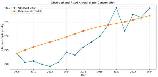
Figure 1 compares the observed annual water-consumption data with the deterministic model solution.

Figure 1. Observed annual domestic water consumption and fitted deterministic model.

The model reproduces the overall long-term behavior of the consumption series and captures the principal variations observed during the study period.

The goodness-of-fit measures are

$$R^2=0.4885,MAE=4.3903,RMSE=5.1550.$$

Although the coefficient of determination is moderate ($R^2=0.4885$), this value should be interpreted in the context of the dataset used in the study. The annual domestic water-consumption series exhibits relatively low variability, with values ranging from 269.16 to 290.17 LPCD and a mean of 278.04 LPCD. In such situations, relatively small deviations from the observed values can produce a noticeable reduction in $R^2$, even when the absolute prediction errors remain modest. For this reason, additional error measures may provide a more informative assessment of model performance.

Using the mean consumption value as a reference, the normalized mean absolute error is approximately $1.58\%$, while the normalized root mean square error is approximately $1.85\%$. These values indicate that the average discrepancy between the observed and predicted consumption levels remains small relative to the magnitude of the data. Consequently, the reported performance measures suggest that the model captures the overall long-term behavior of the annual consumption series reasonably well despite the moderate $R^2$ value.

It should also be noted that the numerical study is based on annual observations covering the period 2008–2024, resulting in a dataset of seventeen observations. The use of annual data is consistent with the objective of the study, which is to investigate long-term water-consumption dynamics under uncertainty rather than short-term forecasting. Therefore, the numerical results should be interpreted within the context of a small annual dataset characterized by relatively limited variability.

5.6. Uncertainty Analysis

The fuzzy model was evaluated by constructing uncertainty bands corresponding to different $\alpha$-levels.

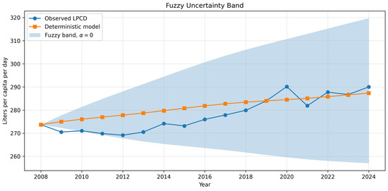
Figure 2 presents the widest uncertainty interval generated by the model, corresponding to $\alpha =0$.

Figure 2. Fuzzy uncertainty band obtained from the proposed model.

The uncertainty band contains 94.12% of the observed data points, indicating that the fuzzy formulation successfully captures a substantial portion of the variability present in the annual consumption series. This result demonstrates that the proposed framework provides meaningful information about the range of plausible consumption values arising from parameter uncertainty.

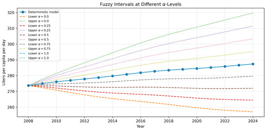
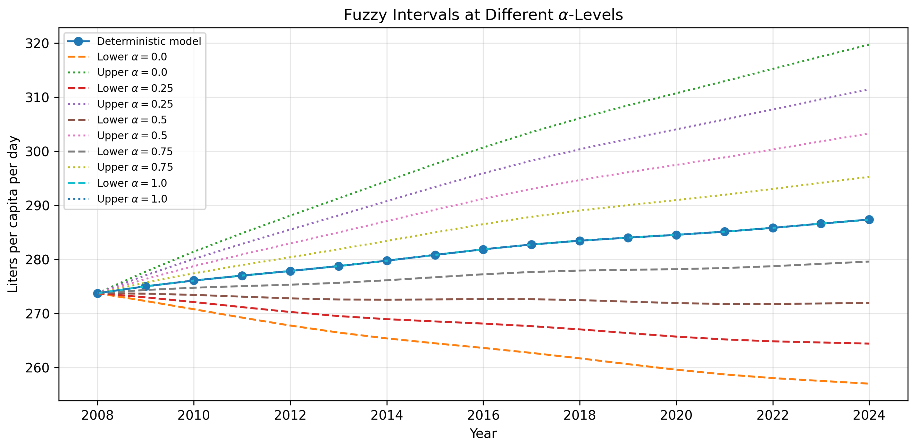
Figure 3 illustrates the interval-valued solutions corresponding to different $\alpha$-levels.

Figure 3. Interval-valued solutions for different $\alpha$-levels.

As predicted by Theorem 3, the uncertainty intervals become progressively narrower as $\alpha$ increases. At $\alpha =1$, the interval collapses to the deterministic solution, while smaller values of $\alpha$ generate wider uncertainty bands that reflect higher levels of uncertainty.

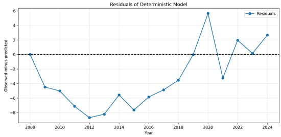
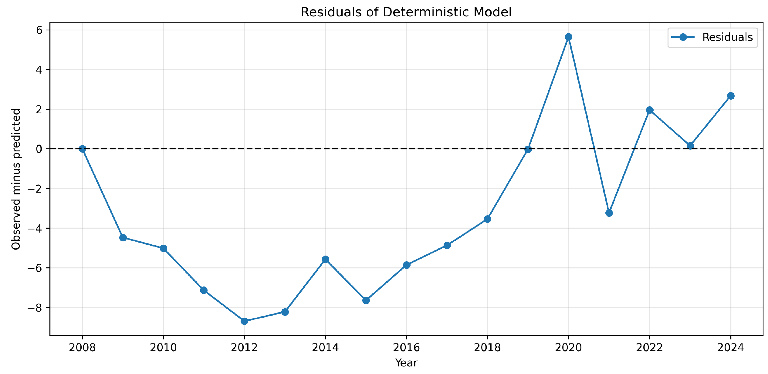
Finally, Figure 4 presents the residuals associated with the deterministic model.

Figure 4. Residuals of the deterministic difference equation model.

The residuals remain bounded throughout the observation period and do not exhibit systematic divergence. This behavior is consistent with the stability and boundedness properties established in Section 4 and further supports the suitability of the proposed model for analyzing long-term water-consumption dynamics.

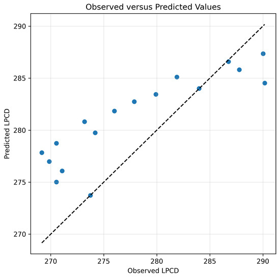
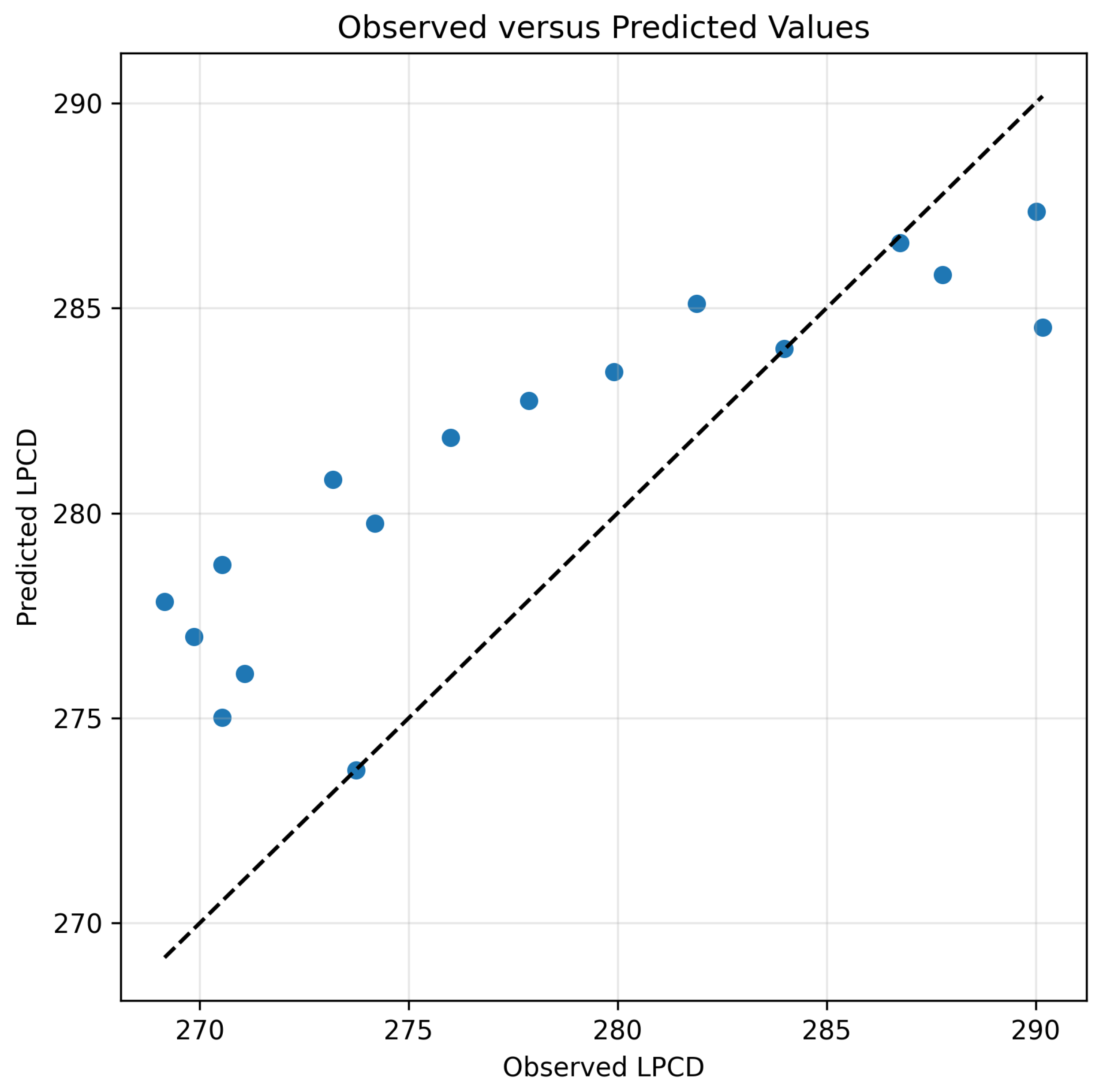
Figure 5 provides an additional assessment of model performance by comparing observed and predicted consumption values. The concentration of points around the diagonal line indicates that the model captures the overall relationship between the observed data and the fitted values, although some deviations remain due to factors not explicitly included in the model.

Figure 5. Observed versus predicted annual domestic water consumption.

6. Discussion

The numerical results show that the proposed fuzzy difference equation model provides a reasonable description of long-term domestic water-consumption dynamics. The estimated parameter $b>0$ indicates a tendency for consumption levels to move toward an equilibrium state, while the periodic forcing terms account for cyclical fluctuations around this level.

The deterministic model achieved an $R^2$ value of 0.4885. Although the model does not capture all sources of variability in the data, it successfully reproduces the overall long-term trend using a relatively simple mathematical structure. Since the objective of this study is to analyze long-term consumption behavior and uncertainty rather than short-term forecasting, the obtained fit is considered satisfactory. An additional observation can be made from the observed-versus-predicted comparison shown in Figure 5. Several points corresponding to lower observed consumption values lie above the diagonal reference line, indicating a tendency of the deterministic model to overestimate consumption during periods when the observed values are relatively low. This behavior is likely related to the mean-reverting structure of the model, which continuously pulls the solution toward the estimated equilibrium level. As a result, unusually low observations may be smoothed toward the long-term average and therefore appear slightly over-predicted, while this tendency represents a limitation of the deterministic formulation, it is not unexpected given the simplicity of the model and its focus on long-term behavior rather than short-term fluctuations. Consequently, the results should be interpreted primarily as a description of long-term consumption dynamics rather than as an attempt to reproduce every variation present in the observed series.

A notable result is the performance of the fuzzy uncertainty analysis. The widest uncertainty band contains 94.12% of the observed data points, indicating that the fuzzy formulation captures a substantial portion of the variability present in the annual consumption series. This demonstrates the usefulness of the proposed framework for quantifying uncertainty in water-consumption dynamics.

The interval-valued solutions also confirm the theoretical results established in Section 4. As the $\alpha$-level increases, the uncertainty intervals become progressively narrower and collapse to the deterministic solution when $\alpha =1$. This behavior illustrates the consistency between the theoretical and numerical components of the model.

Several limitations should be noted. The analysis is based on an aggregated annual dataset containing only seventeen observations, which restricts the complexity of the model that can be reliably estimated. In addition, the current framework considers uncertainty only through fuzzy parameters and does not explicitly incorporate external factors such as climate conditions, economic variables, or population growth.

Future research may extend the proposed approach by incorporating additional explanatory variables, developing multi-region fuzzy difference equation models, or combining fuzzy dynamical systems with machine learning techniques. Such extensions may provide a more detailed representation of water-consumption dynamics while preserving the uncertainty quantification capabilities of the proposed framework.

7. Conclusions

Water-consumption data are often affected by uncertainty, particularly when observations are aggregated over long periods and precise parameter values are difficult to determine. This study explored how a fuzzy difference equation framework can be used to represent that uncertainty while still providing a simple description of the underlying consumption dynamics.

Using annual domestic water-consumption data from Taiwan, the proposed model was able to reproduce the general behavior of the observed series and generate uncertainty bands around the deterministic solution. The numerical results showed that the fuzzy formulation provides additional information beyond a single fitted trajectory by describing a range of plausible outcomes associated with uncertainty in the model parameters.

From a mathematical perspective, the analysis established several properties of the model and showed that the interval structure of the fuzzy solution is preserved throughout the evolution of the system. The numerical simulations were consistent with these theoretical findings and illustrated how uncertainty changes over time under the proposed dynamics.

The model considered in this paper is intentionally simple. Its purpose is not to provide highly accurate forecasts but rather to offer an interpretable framework for studying long-term consumption behavior when uncertainty cannot be ignored. Despite its simplicity, the results suggest that fuzzy difference equations can provide useful insight into water-consumption dynamics and may serve as a foundation for more detailed models.

There are several directions in which this work can be extended. Future studies may incorporate additional variables that influence water consumption, investigate regional differences through multi-area models, or combine the proposed framework with other modeling approaches. Such developments may lead to a richer understanding of water-consumption patterns while retaining the ability to account for uncertainty in a systematic way.

References

- Maidment, D.R.; Miaou, S.-P. Daily water use in nine cities. Water Resour. Res. 1986, 22, 845–851. [Google Scholar] [CrossRef] [Scilit]
- Jain, A.; Ormsbee, L.E. Short-term water demand forecast modeling techniques. J. AWWA 2002, 94, 64–72. [Google Scholar] [CrossRef] [Scilit]
- Herrera, M.; Torgo, L.; Izquierdo, J.; Pérez-García, R. Predictive models for forecasting hourly urban water demand. J. Hydrol. 2010, 387, 141–150. [Google Scholar] [CrossRef] [Scilit]
- House-Peters, L.A.; Chang, H. Urban water demand modeling: Review of concepts, methods, and organizing principles. Water Resour. Res. 2011, 47, W05401. [Google Scholar] [CrossRef] [Scilit]
- Donkor, E.A.; Mazzuchi, T.A.; Soyer, R.; Roberson, J.A. Urban water demand forecasting: Review of methods and models. J. Water Resour. Plan. Manag. 2014, 140, 146–159. [Google Scholar] [CrossRef] [Scilit]
- Romano, M.; Kapelan, Z. Adaptive water demand forecasting for near real-time management of smart water distribution systems. Environ. Model. Softw. 2014, 60, 265–276. [Google Scholar] [CrossRef] [Scilit]
- Adamowski, J.; Chan, H.F.; Prasher, S.O.; Ozga-Zielinski, B.; Sliusarieva, A. Comparison of multiple linear and nonlinear regression, autoregressive integrated moving average, artificial neural network, and wavelet artificial neural network methods for urban water demand forecasting in Montreal, Canada. Water Resour. Res. 2012, 48, W01528. [Google Scholar] [CrossRef] [Scilit]
- Oyebode, O.; Ighravwe, D.E. Urban water demand forecasting: A comparative evaluation of conventional and soft computing techniques. Resources 2019, 8, 156. [Google Scholar] [CrossRef] [Scilit]
- Pacchin, E.; Gagliardi, F.; Alvisi, S.; Franchini, M. A comparison of short-term water demand forecasting models. Water Resour. Manag. 2019, 33, 1481–1497. [Google Scholar] [CrossRef] [Scilit]
- Niknam, A.; Zare, H.K.; Hosseininasab, H.; Mostafaeipour, A.; Herrera, M. A critical review of short-term water demand forecasting tools: What method should I use? Sustainability 2022, 14, 5412. [Google Scholar] [CrossRef] [Scilit]
- Ghannam, S.; Hussain, F. Short-term water demand forecasting: A review. Australas. J. Water Resour. 2024, 1–19. [Google Scholar] [CrossRef] [Scilit]
- Zadeh, L.A. Fuzzy sets. Inf. Control 1965, 8, 338–353. [Google Scholar] [CrossRef] [Scilit]
- Dubois, D.; Prade, H. Fuzzy Sets and Systems: Theory and Applications; Academic Press: New York, NY, USA, 1980. [Google Scholar]
- Zimmermann, H.-J. Fuzzy Set Theory and Its Applications, 4th ed.; Springer: New York, NY, USA, 2001. [Google Scholar]
- Ross, T.J. Fuzzy Logic with Engineering Applications, 4th ed.; Wiley: Hoboken, NJ, USA, 2017. [Google Scholar]
- Pedrycz, W.; Gomide, F. An Introduction to Fuzzy Sets: Analysis and Design; MIT Press: Cambridge, MA, USA, 1998. [Google Scholar]
- Klir, G.J.; Yuan, B. Fuzzy Sets and Fuzzy Logic: Theory and Applications; Prentice Hall: Upper Saddle River, NJ, USA, 1995. [Google Scholar]
- Yager, R.R.; Filev, D.P. Essentials of Fuzzy Modeling and Control; Wiley: New York, NY, USA, 1994. [Google Scholar]
- Kaleva, O. Fuzzy differential equations. Fuzzy Sets Syst. 1987, 24, 301–317. [Google Scholar] [CrossRef] [Scilit]
- Puri, M.L.; Ralescu, D.A. Fuzzy random variables. J. Math. Anal. Appl. 1986, 114, 409–422. [Google Scholar] [CrossRef] [Scilit]
- Buckley, J.J.; Feuring, T. Fuzzy differential equations. Fuzzy Sets Syst. 2000, 110, 43–54. [Google Scholar] [CrossRef] [Scilit]
- Bede, B.; Gal, S.G. Generalizations of the differentiability of fuzzy-number-valued functions with applications to fuzzy differential equations. Fuzzy Sets Syst. 2005, 151, 581–599. [Google Scholar] [CrossRef] [Scilit]
- Stefanini, L.; Bede, B. Generalized Hukuhara differentiability of interval-valued functions and interval differential equations. Nonlinear Anal. Theory Methods Appl. 2009, 71, 1311–1328. [Google Scholar] [CrossRef] [Scilit]
- Bede, B. Mathematics of Fuzzy Sets and Fuzzy Logic; Springer: Berlin/Heidelberg, Germany, 2013. [Google Scholar]
- Alvisi, S.; Franchini, M. Fuzzy neural networks for water level and discharge forecasting with uncertainty. Environ. Model. Softw. 2011, 26, 523–537. [Google Scholar] [CrossRef] [Scilit]
- Chang, F.J.; Chang, L.C.; Huang, C.W.; Kao, I.F. Prediction of monthly regional groundwater levels through hybrid soft-computing techniques. J. Hydrol. 2016, 541, 965–976. [Google Scholar] [CrossRef] [Scilit]
- Nayak, P.C.; Sudheer, K.P.; Ramasastri, K.S.; Rangan, D.M. Fuzzy computing based rainfall-runoff model for real-time flood forecasting. Hydrol. Process. 2005, 19, 955–968. [Google Scholar]
- Kambalimath, S.; Deka, P.C. A basic review of fuzzy logic applications in hydrology and water resources. Appl. Water Sci. 2020, 10, 191. [Google Scholar] [CrossRef] [Scilit]
- Taiwan Government Open Data Platform. Statistical Data on Domestic Water Usage. Available online: https://data.gov.tw/en/datasets/8316 (accessed on 6 June 2026).
Disclaimer/Publisher’s Note: The statements, opinions and data contained in all publications are solely those of the individual author(s) and contributor(s) and not of MDPI and/or the editor(s). MDPI and/or the editor(s) disclaim responsibility for any injury to people or property resulting from any ideas, methods, instructions or products referred to in the content. |
© 2026 by the author. Licensee MDPI, Basel, Switzerland. This article is an open access article distributed under the terms and conditions of the Creative Commons Attribution (CC BY) license.