


Abstract
This study presents a comprehensive symmetry-breaking analysis framework for a twelve-legged Jansen walking robot, integrating finite element analysis (FEA) with adaptive neuro-fuzzy inference system (ANFIS) surrogate modeling. A systematic dataset of 210 cases was generated by combining 21 single- and multi-leg failure scenarios across 10 load levels (20–200 N) on the PLA-based 3D-printed prototype. Two novel dimensionless metrics are introduced: the Resilience Index (RI), quantifying the proportional stress increase relative to the baseline, and the Asymmetry Index (AI), measuring leg-reaction force distribution imbalance. Results identify a clear fault-tolerance threshold between two- and four-leg failures: single-leg failures remain at LOW risk (RI < 0.20), while three-leg asymmetric failures (S18) reach CRITICAL level (RI = 1.13, ~97% of PLA yield strength). A hybrid machine learning framework is proposed, applying ANFIS to maximum stress (R2 = 0.817) and safety factor (R2 = 0.936) predictions, while reserving FEA tables for bimodal outputs. The ANFIS surrogate achieves approximately 106× speedup over FEA (262.6 μs vs. 5–8 min), enabling real-time fault diagnosis and digital twin applications. The framework is generalizable to other multi-legged robotic systems requiring fault-tolerance evaluation.
1. Introduction
Multi-legged walking robots have emerged as one of the fastest-growing subfields in mobile robotics research over the past decade. Unlike wheeled systems, these platforms offer high maneuverability on uneven terrain, static stability, fault tolerance through multiple contact points, and minimal ground contact on sensitive surfaces [1,2]. These advantages make multi-legged robots well-suited for critical applications, such as search-and-rescue operations, agricultural monitoring, military reconnaissance, planetary surface exploration, and industrial pipeline inspection [3,4]. In such applications, preserving the ability to complete a mission even when one or more legs fail (fault tolerance) becomes vital—especially in environments inaccessible or hazardous to humans. Systematic modeling of how leg failures affect structural behavior has therefore become a central research question in multi-legged robot design [5].
The Strandbeest mechanism developed by Theo Jansen is an elegant engineering solution: a single-degree-of-freedom linkage that produces natural walking-like trajectories at the foot tip [6,7]. Driving multiple legs in a synchronized pattern from a single motor input affords the mechanism notable advantages in energy efficiency and control simplicity [8]. The literature on Jansen-type mechanisms covers kinematic analysis [9,10], trajectory optimization [11], dynamic characterization [12,13], and energy efficiency improvement [14]. However, most of these studies focus on conventional six- or eight-legged configurations; the structural behavior of twelve-legged variants—particularly under leg-failure scenarios—has received very limited attention [15]. While increasing the number of legs improves static stability margins and load distribution across multiple support points, it also exponentially expands the set of possible failure combinations and complicates the structural response under symmetry breaking. This gap becomes especially pronounced in 3D-printed PLA prototypes, where the material’s strength limits define the practical design envelope [16].
Symmetry is a foundational principle in engineering design: in structural systems, symmetric load distribution minimizes stress concentrations and produces predictable mechanical behavior [17]. Under real operational conditions, however, events such as leg failure, motor malfunction, sensor faults, or ground irregularity disrupt the design’s symmetry and trigger a critical phenomenon known as symmetry breaking [18,19]. Mechanically, symmetry breaking manifests as local stress concentrations, asymmetric load transfer, body torsion, and chassis tilting [20]. Although the concept has been studied extensively in physics [21], structural mechanics [22,23], and biomechanical systems [24], no standard metric framework currently exists for quantifying symmetry breaking in multi-legged robotic platforms. Existing work remains largely qualitative; comparable, dimensionless, and universal indicators that could guide design decisions have not been proposed [25]. This absence prevents objective fault-tolerance comparison across different multi-legged designs.
Finite element analysis (FEA) is regarded as the gold standard for structural evaluation, but each scenario typically requires minutes to hours of computation [26]. This limitation poses a serious bottleneck for real-time applications, online fault diagnosis, and digital twin architectures [27]. Machine learning-based surrogate models have been proposed to overcome this challenge. Among them, the Adaptive Neuro-Fuzzy Inference System (ANFIS) stands out as a powerful approach that combines the data-driven learning capacity of neural networks with the rule-based interpretability of fuzzy logic [28,29]. ANFIS models have been successfully applied across engineering domains, including structural health monitoring [30], seismic response prediction [31], composite material behavior [32], and mechanical design optimization [33]. However, the use of ANFIS for fault-tolerance prediction in multi-legged robotic platforms has not been systematically addressed in the literature. This gap motivates the development of a framework that integrates symmetry-breaking metrics with real-time predictive capabilities.
The preceding review reveals three specific gaps: (i) the structural behavior of high-redundancy twelve-legged walkers under leg-failure scenarios remains largely unexplored, in contrast to the well-studied six- and eight-legged configurations; (ii) no dimensionless, transferable metrics exist for quantifying symmetry-breaking severity independently of absolute load magnitude; and (iii) an integrated FEA-driven surrogate framework enabling real-time fault diagnosis for multi-legged systems has not been established. To address these gaps, this study introduces a hybrid FEA-ANFIS framework that systematically analyzes the structural impact of single- and multi-leg failure scenarios on a twelve-legged Jansen walker. A total of 210 finite element analyses were performed by combining 21 failure scenarios with 10 load levels, producing—to our knowledge—the first comprehensive structural dataset for a twelve-legged Jansen walker covering single, diagonal, same-side, group, and multi-leg failure modes across the 20–200 N load range. A second contribution is the introduction of two new dimensionless symmetry-breaking metrics: the Resilience Index (RI), which quantifies the proportional increase in maximum stress relative to the baseline, and the Asymmetry Index (AI), which measures the redistribution imbalance of leg-reaction forces. We further propose a hybrid surrogate modeling framework in which the most suitable machine learning method is selected per output based on its statistical characteristics: ANFIS models were applied to maximum stress (, R2 = 0.817) and safety factor (SF, R2 = 0.936), while FEA tables were retained for outputs with lower-frequency or bimodal distributions (maximum deformation and tilt angle θ). The study also evaluates four-leg group failures (S15 and S16) as boundary cases, quantifying the linear-elastic limit of the PLA chassis and the fault-tolerance threshold. The proposed FEA-ANFIS framework is not specific to the platform studied here; it is presented as a general methodology that can be directly applied to fault-tolerance evaluation of other multi-legged robotic systems. ANFIS inference is approximately 106 times faster than FEA simulation, which provides practical value for real-time fault diagnosis and digital twin applications.
2. Materials and Methods
2.1. Robot Configuration
The system studied here is a twelve-legged walking robot built around the Strandbeest mechanism and produced as a 3D-printed PLA prototype (Figure 1). The structure features two independent drive motors placed symmetrically around a central PLA chassis. Each motor drives six legs on its own side through a gearbox: motor M1 actuates the six left legs (L1–L6), while motor M2 actuates the six right legs (R1–R6) (Figure 1a). The base mechanical design was adapted from a publicly available Strandbeest CAD model [34], with modifications to the chassis geometry, motor mounting plates, and connection details; however, the leg-link lengths were preserved at the original Jansen proportions. This configuration provides a two-stage symmetric drive arrangement between the left and right sides.
Figure 1.
Configuration of the twelve-legged Jansen walker. (a) Top view: leg numbering scheme; the eight legs shown in green represent the ground-contact fixed support points, while the four legs shown in brown indicate the free/airborne legs in the orbital cycle. (b) Isometric view: 3D CAD model of the entire structure; two independent motor systems and the chassis body are visible. (c) Two-legged side view: detailed view of the leg pair on one side; the gear mechanism, lever, and eleven Jansen connection elements are visible.
Each leg consists of eleven linkage elements that form the classical Jansen mechanism, which produces a natural walking-like foot trajectory from a single rotational input. The detailed structure of a single-leg mechanism is shown in Figure 1c, where the drive gear and all linkage elements are clearly visible. The legs are arranged in a two-row × three-column layout on each side: front-row legs are L1, L2, L3 (left) and R1, R2, R3 (right); rear-row legs are L4, L5, L6 (left) and R4, R5, R6 (right) (Figure 1a). The rotational phase distribution of the legs ensures that at any given moment, eight of the twelve legs are in ground contact, while the remaining four are airborne in their orbital cycle. This natural asynchronous operation guarantees that the walker is always supported at multiple points and remains statically stable.
In the static analysis configuration studied here, the eight ground-contact legs are: L2, L3, L4, L5, R1, R2, R5, and R6 (shown in green in Figure 1a). The four airborne legs in the orbital cycle are L1, L6, R3, and R4 (shown in brown). In the structural analysis, only the eight ground-contact legs were modeled as mechanical support points; the airborne legs were suppressed in the ANSYS 2024 R2 finite element model because they do not contribute to structural load transfer. This approach accurately represents the instantaneous load distribution at the static equilibrium configuration.
The chassis is the main load-bearing structural element of the robot and connects the two side motor mounting plates. The measured chassis width is W = 95.76 mm, which is used as the reference length in the tilt angle (θ) calculation defined in the symmetry-breaking analysis (see Section 2.6.4). All structural components were fabricated from PLA via 3D printing. The printing parameters and mechanical properties of the material are detailed in Section 2.2.
2.2. Material Properties and Manufacturing Parameters
The structural components of the robot were produced from polylactic acid (PLA) filament via additive manufacturing. PLA is a thermoplastic polymer derived from renewable sources, biodegradable, and with a low environmental footprint; it is widely preferred for prototyping applications due to its ease of processing, low cost, broad availability, and consistent print quality. The printing parameters used in this study are summarized in Table 1.
Table 1.
3D printing production parameters for PLA components.
The isotropic homogeneous assumption is adopted for three reasons. First, the components carry loads distributed across multiple print directions, averaging the directional stiffness variation that characterizes FDM parts. Second, at the low infill density used in this study, the influence of layer-to-layer anisotropy on the global stiffness is reduced relative to fully dense prints, and remains secondary to the geometric stress concentrations that govern the failure scenarios [16]. Third, using the manufacturer-reported isotropic yield strength provides a conservative safety estimate. Crucially, since the RI and AI metrics are proportional ratios relative to the baseline, any anisotropic effect present in both the baseline and failure scenarios largely cancels out, leaving the symmetry-breaking conclusions unaffected. Full anisotropic characterization is identified as future work (Section 4.2).
To quantitatively assess the influence of material anisotropy, a sensitivity analysis was performed on the baseline scenario (S0) at 200 N by replacing the isotropic model with an orthotropic formulation representative of flat-printed FDM-PLA. The in-plane modulus was set equal to the bulk PLA value (3500 MPa), and the build-direction modulus was reduced by approximately 17% (2900 MPa), consistent with the build-orientation stiffness reduction reported for FDM-PLA (a longitudinal-to-bulk reduction of about 16.6% is documented in the literature) [35]; the weak build-direction axis was deliberately aligned with the primary loading direction to represent the worst case. The orthotropic parameters are listed in Table 2.
Table 2.
Orthotropic material parameters used in the sensitivity analysis, representative of flat-printed FDM-PLA.
The resulting maximum stress (22.40 MPa) deviates by only 3.3% from the isotropic prediction (23.16 MPa), and the maximum deformation by 7.6% (1.67 mm vs. 1.56 mm), as summarized in Table 3. Notably, the isotropic model yields a slightly higher stress, confirming that it provides a conservative estimate for safety-factor evaluation. This small deviation—obtained under a worst-case orientation—reflects the near-isotropic mechanical behavior characteristic of the gyroid infill pattern, and confirms that the isotropic assumption does not materially affect the fault-tolerance conclusions.
Table 3.
Sensitivity of baseline structural response to the material model assumption (S0, 200 N, worst-case orientation).
The mechanical properties of PLA used in the finite element analysis were defined based on standard values reported in the literature for 3D-printed PLA [16]. Although a low infill density (10%) was chosen in this study, the material was modeled as an equivalent isotropic continuum in the ANSYS finite element model; the effect of the reduced infill on effective mechanical properties was neglected, adopting a conservative design approach. This assumption is widely used in the literature for structural evaluations where anisotropic effects and infill geometry are excluded from the analysis [16]. The mechanical properties used in the model are listed in Table 4.
Table 4.
PLA material properties used in the ANSYS finite element model.
Material-Property Uncertainty Analysis
To evaluate the effect of uncertainty in the mechanical properties of the manufactured FDM-PLA components, a Monte Carlo-based uncertainty analysis was performed. Young’s modulus and yield strength were varied by ±10% around their nominal values of 3500 MPa and 50 MPa, respectively. A total of 10,000 random samples were generated within these limits.
The analysis was applied to representative scenarios from the 200 N load case, including the baseline condition, single-leg failure, two-leg failure, near-critical multi-leg failure, and boundary group-failure cases. The nominal FEA stress values were kept unchanged, while the safety factor and deformation response were recalculated for each sampled material condition. The probability of yielding was then estimated from the percentage of samples in which the safety factor fell below unity.
2.3. Finite Element Method
ANSYS Workbench 2024 R2 (Static Structural module) was used for the structural analysis in this study. The analyses were configured as linear-static because PLA exhibits linear-elastic behavior at the load levels examined.
The CAD model created in SolidWorks 2024 was imported into ANSYS Mechanical, where the connections between components were modeled as rigid (bonded) contacts. The four airborne legs in the orbital cycle (L1, L6, R3, R4) were suppressed in the model because they do not carry structural load; the eight ground-contact legs (L2, L3, L4, L5, R1, R2, R5, R6) were preserved as active structural support points.
The mesh was generated using SOLID186 elements—20-node quadratic solid elements commonly preferred for complex 3D geometries. A global element size of 5 mm was specified, complemented by an additional body sizing of 5 mm applied separately to ensure consistent discretization across all bodies. The resulting mesh contains 211,012 nodes and 408,332 elements. This resolution provides sufficient discretization of the structural stress field, as verified by the mesh convergence study presented in Section Mesh Convergence Study. This resolution provides sufficient discretization of the structural stress field.
The Sparse Direct Solver was used for the solutions, with a typical solution time of approximately 5–8 min per scenario. The total computation time for all 210 scenarios was approximately 17–28 h.
Mesh Convergence Study
A comprehensive mesh convergence study was conducted on the baseline scenario (S0) at the maximum load level of 200 N to verify the reliability of the finite element predictions. Twenty mesh refinement levels were evaluated, spanning global element sizes from 10 mm to 4 mm, with the body sizing set to match the global element size in each case. The maximum von Mises stress (σmax) was recorded for each mesh.
The results, summarized in Table 5 and visualized in Figure 2, identify three distinct regimes. In the under-resolved regime (element size > 5.8 mm), σmax increases monotonically from 13.56 MPa at 10 mm to 17.13 MPa at 5.8 mm, as the coarse mesh fails to capture the local stress gradients near the connection points of the Jansen linkages. In the transition regime (5.0–5.8 mm), σmax rises sharply as the discretization progressively resolves the stress-concentration features. In the converged regime (element size ≤ 5.0 mm, eleven refinement levels), σmax stabilizes at 23.78 ± 0.38 MPa, with a coefficient of variation of only 1.6%.
Table 5.
Mesh convergence study for the baseline scenario (S0) at 200 N, spanning 20 element sizes from 10 mm to 4 mm. In the converged regime (≤5.0 mm), σmax = 23.78 ± 0.38 MPa (CV = 1.6%). The 5 mm element size used in this study deviates by only 2.6% from the asymptotic mean.
Figure 2.
Mesh convergence analysis showing the variation in maximum von Mises stress (σmax) with element size for the baseline scenario at 200 N, across 20 refinement levels. Three regimes are visible: under-resolved (>5.8 mm), transition (5.0–5.8 mm), and converged (≤5.0 mm). The 5 mm element size used in this study (gold star) lies at the entry of the converged region, deviating only 2.6% from the asymptotic mean (23.78 MPa).
The 5 mm element size used throughout this study yields σmax = 23.16 MPa, deviating by only 2.6% from the asymptotic mean of the converged regime—well within the commonly accepted 5% convergence threshold for static structural simulations of complex assemblies [26]. Mesh independence is therefore established for the 5 mm configuration adopted in all 210 analyses. Given that the full 210-case computation required approximately 17–28 h at the 5 mm resolution, further refinement was not pursued in order to maintain a practical balance between numerical accuracy and computational cost.
2.4. Boundary Conditions and Loading
Two main boundary conditions govern the structural behavior in the finite element model: definition of the leg supports and application of the external load (Figure 3).
Figure 3.
Boundary conditions and loading scheme. Fixed supports were applied to the bottom surfaces of the eight legs in contact with the ground; the external load was applied in the −Y direction as a force (20–200 N) distributed across the center of the chassis.
The bottom surfaces of the eight ground-contact legs (L2, L3, L4, L5, R1, R2, R5, R6) were defined as fixed supports, constraining all rotational and translational degrees of freedom on these surfaces. This represents the static equilibrium configuration in which the legs are in full contact with the ground.
The external load was applied as a distributed force on the chassis center in the −Y direction. This loading represents the operational carrying capacity of the robot. To ensure consistency across scenarios, only the load magnitude was varied; the application point and direction were kept constant in all analyses.
The load magnitude was parameterized at ten levels, from 20 N to 200 N in increments of 20 N. This range was selected to verify the linear-elastic behavior of the material at low loads and to reveal potential critical stress concentrations at higher loads. In total, 21 failure scenarios × 10 load levels = 210 finite element analyses were performed.
2.5. Failure Scenario Design
Twenty-one failure scenarios were defined to systematically evaluate the fault tolerance of the twelve-legged walker. The scenarios are organized into seven categories to represent different structural modes of symmetry breaking: baseline, single, diagonal, same-side, group, front-axis, and multi-leg failures. This classification captures both the physical mechanism of symmetry breaking and the practical failure modes likely to occur in operation.
The scenarios are defined only over the eight ground-contact legs (L2, L3, L4, L5, R1, R2, R5, R6); the airborne legs in the orbital cycle (L1, L6, R3, R4) were not included in the failure modeling because they do not carry structural load (Figure 4). In each scenario, the legs marked as “failed” were suppressed in the ANSYS model and their corresponding fixed support conditions removed; this represents the loss of structural support from those legs. The full list of scenarios is presented in Table 6.
Figure 4.
Top view schematic diagram: eight legs in contact with the ground (green) and four legs in the air (gray). Failure scenarios are defined only for the green legs. The M1 and M2 motors at the center of the chassis drive the left and right legs, respectively. The chassis width W = 95.76 mm and is used as the reference length in slope angle (θ) calculations.
Table 6.
A description of the 21 failure scenarios examined in this study.
S0 (Baseline) represents the reference case in which all legs are intact. It defines the baseline structural response for all subsequent comparisons and serves as the reference value in the symmetry-breaking metric calculations (Section 2.6).
Single-leg failures (S1–S8) cover cases in which only one of the ground-contact legs fails. Four scenarios are defined on the left side (S1–S4) and four on the right side (S5–S8); this group is used to examine the structural impact of low-level symmetry breaking.
Diagonal failures (S9–S11) represent simultaneous failures of legs located on opposite sides of the robot. These scenarios are important for evaluating diagonal load transfer and its effect on structural balance.
Same-side failures (S12–S14) involve the simultaneous failure of two adjacent legs on the same side. This group was considered to study lateral symmetry breaking and chassis tilting behavior.
Group failures (S15, S16) represent the boundary cases in which all ground-contact legs on one side fail simultaneously. S15 corresponds to full left-side failure (L2 + L3 + L4 + L5), and S16 to full right-side failure (R1 + R2 + R5 + R6). Because the stress obtained in these scenarios substantially exceeds the PLA yield strength ( = 50 MPa), they are discussed separately in Section 3.4.
Front-axis and multi-leg failures (S17–S20) include more complex failure combinations. S17 represents a bilateral failure on the front legs, while S18–S20 represent three-leg multi-failure cases. These scenarios allow evaluation of the structural response under the multi-failure conditions that may occur in practical applications.
2.6. Quantifying Symmetry Breaking
Four metrics are used in this study to quantify the symmetry breaking caused by structural failure conditions. Of these, the Resilience Index (RI) and Asymmetry Index (AI) are two new metrics introduced in this work, while the Safety Factor (SF) and tilt angle (θ) are standard indicators commonly used in structural evaluation. The conceptual structure of RI and AI is summarized schematically in Figure 5. All metrics can be computed directly from the ANSYS finite element output.
Figure 5.
Conceptual schematic of the two new symmetry-breaking metrics introduced in this study. The Resilience Index (RI) measures structural resilience by quantifying the proportional increase in maximum stress relative to the baseline (S0). The Asymmetry Index (AI) reflects the distribution imbalance of reaction forces among the ground-contact legs.
2.6.1. Resilience Index (RI)
The Resilience Index (RI) is a dimensionless metric that measures the proportional increase in the maximum stress observed in a failure scenario relative to the baseline (S0) condition. It is proposed in this study to quantify the sensitivity of structural resilience to failure severity. RI is computed from Equation (1):
Here, σmax,Si denotes the maximum von Mises stress (MPa) computed in the i-th failure scenario, and ,S0 represents the maximum stress computed in the baseline condition at the same load level. RI has a direct physical interpretation: RI = 0 corresponds to a structural response equivalent to the baseline, while RI = 1 indicates a maximum stress that has doubled relative to the baseline.
Based on RI values, the structural risk level is classified on a four-level scale (Table 7):
Table 7.
Risk classification based on the Resilience Index (RI).
The four-level RI classification is justified on three grounds. First, on theoretical grounds, the thresholds map to specific safety-factor reservations: given the baseline SF = 2.63, the thresholds RI = 0.20, 0.50, and 1.00 correspond to SF = 2.19, 1.75, and 1.32, respectively, with RI = 1.00 marking the point where σmax approaches the PLA yield strength (50 MPa) and the structure exits the linear-elastic envelope. Second, the bands (20%, 50%, and 100% increases over baseline) coincide with the standard degradation thresholds used in dependability and fault-tolerant systems analysis [25]. Third, the thresholds are supported by the empirical RI distribution across failure-severity classes (Figure 6): single-leg failures (S1–S8) fall almost entirely within the LOW band (third quartile = 0.11; 87.5% below RI = 0.20), two-leg failures (S9–S14) span the MEDIUM–HIGH range, and three-leg failures (S18, S20) reach the CRITICAL band. Within the fault-tolerant operating envelope (S1–S14 and S18, S20; excluding boundary cases S15–S16, which exceed the linear-elastic limit), the largest natural gap in the sorted RI values occurs at 0.53 → 1.13 (gap = 0.60), coinciding with the HIGH–CRITICAL boundary. The group-failure scenarios S15 and S16 (RI = 7.17 and 6.08) constitute a qualitatively distinct category that lies beyond the linear-elastic design envelope and are treated as boundary cases throughout this study. An analogous three-tier rationale applies to the Asymmetry Index, whose values correlate strongly with RI (Pearson r = 0.87), confirming that the two metrics are complementary indicators of symmetry-breaking severity.
Figure 6.
Distribution of the Resilience Index (RI) across three failure-severity classes at 200 N. The proposed thresholds (RI = 0.20, 0.50, 1.00) align with the natural separation between classes within the fault-tolerant operating envelope. Group-failure scenarios S15 and S16 (RI = 7.17 and 6.08) are excluded as they exceed the linear-elastic design limit (see Section 3.5).
2.6.2. Asymmetry Index (AI)
The Asymmetry Index (AI) is a dimensionless metric that measures the distribution imbalance of reaction forces among the ground-contact legs. Under the baseline condition, the load is distributed evenly; following a leg failure, the load is asymmetrically redistributed to the remaining support points. AI quantifies this imbalance according to Equation (2):
Here, and are the maximum and minimum reaction forces (N) among the ground-contact legs, and is the mean reaction force across all active legs. Values of AI near zero represent a perfect symmetric load distribution, while high values indicate significant load concentration.
RI measures the severity of the structural response, whereas AI measures the uniformity of load distribution. The two metrics are complementary: high RI values point to critical stress concentrations, while high AI values indicate that the design transfers load unevenly to the remaining legs.
2.6.3. Safety Factor (SF)
The Safety Factor (SF) is defined as the ratio of the material’s yield strength to the computed maximum stress, as given in Equation (3):
Here, = 50 MPa is the PLA yield strength defined in Section 2.2, and is the maximum von Mises stress computed in the corresponding scenario. SF > 1 indicates that the structure operates within the elastic limit, while SF ≤ 1 indicates that the material has reached or exceeded yielding. This metric provides a directly usable indicator for classical structural safety assessment and constitutes one of the prediction targets of the ANFIS surrogate model trained in Section 2.7.
2.6.4. Tilt Angle (θ)
The chassis tilt angle (θ) is defined as the geometric indicator of symmetry breaking. It is computed from the difference in vertical displacements at two symmetric reference points on the chassis (Equation (4)):
Here, , R and , L are the vertical displacements (mm) computed at symmetric reference points on the right and left edges of the chassis, and W = 95.76 mm is the chassis width defined in Section 2.1. Positive values represent a rightward tilt, while negative values represent a leftward tilt.
Unlike conventional stress-based metrics, the tilt angle is a visual and operational indicator of symmetry breaking; it represents a physical parameter that an observer could visually assess as the robot tilting to one side. In this study, θ values were categorically classified in Section 3.7 to provide directional information on symmetry breaking.
2.7. Hybrid Machine Learning Surrogate Model
While finite element analysis (FEA) can examine structural behavior with high accuracy, it does not deliver predictions fast enough for real-time applications and digital twin systems [27]. In the 210-case dataset used in this study, each analysis took approximately 5–8 min, bringing the total solution time to 17–28 h. To mitigate this issue, machine learning-based surrogate models were developed from the FEA data, enabling millisecond-scale prediction of structural responses [36]. The literature reports that methods such as artificial neural networks and polynomial regression have produced successful results in stress prediction [37,38].
A hybrid machine learning approach was applied in this study, taking into account the statistical characteristics of the output variables. Instead of a single model, the most suitable method was selected for each output (Table 8). This approach is based on the “right model for the right variable” principle.
Table 8.
Hybrid ML modeling strategy for the four target outputs.
ANFIS was used for σmax and SF, which show a smooth, continuous relationship with load. In contrast, δmax and θ exhibited different behaviors. δmax shows a bimodal distribution caused by regime changes tied to failure severity, while θ remains at low values in single-leg failures, falling below the geometric noise floor. For these two outputs, ANFIS therefore did not provide sufficient accuracy, and the results were reported in tabular form directly from the FEA simulation data. A detailed evaluation of these outputs is given in Section 3.7 and Section 3.8.
2.7.1. ANFIS Architecture
The Adaptive Neuro-Fuzzy Inference System (ANFIS), proposed by Jang [28], is a hybrid model that combines the learning capacity of artificial neural networks with the rule-based inference power of fuzzy logic [29]. ANFIS has a five-layer structure that represents the Sugeno-type fuzzy inference system within a neural network architecture (Figure 7):
Figure 7.
The five-layer structure of ANFIS: fuzzification, rule firing, normalization, consequent computation, and aggregation layers.
Layer 1 (Fuzzification): Input variables are converted into fuzzy sets through membership functions. Gaussian membership functions were used in this study.
Layer 2 (Rule Firing): The firing strength of each rule is computed as the product of the input membership degrees.
Layer 3 (Normalization): Firing strengths are normalized as a ratio of the total firing strength.
Layer 4 (Consequent): The output contribution of each rule is multiplied by the corresponding consequent function (a linear combination in Sugeno-type systems).
Layer 5 (Aggregation): All normalized rule outputs are summed to produce the final numerical prediction.
ANFIS uses a hybrid learning algorithm: parameters are updated in two stages during training—premise parameters via Least Squares Estimation (LSE) and consequent parameters via backpropagation [28]. The interpretable, rule-based structure of ANFIS and its ability to capture nonlinear relationships have enabled its successful use in diverse engineering applications, including structural health monitoring [30,31], material behavior [32], composite materials [33], and medical diagnosis systems [39].
2.7.2. Input Characteristics and Data Preparation
Four input features were defined for the ANFIS models:
- -
- Applied external load (20–200 N);
- -
- Number of failed legs (0–4);
- -
- Asymmetry: Absolute difference between left- and right-side failures (| − |);
- -
- Failure_type: Failure category code (0 = baseline, 1 = single, 2 = diagonal, 3 = same-side, 4 = group, 5 = front-axis, 6 = multi).
These features represent physically meaningful inputs rather than raw scenario identifiers, allowing the model to directly learn the structural impact of failure patterns. In structural surrogate modeling, physically meaningful feature engineering has been reported to significantly improve prediction accuracy compared with raw parameters alone [37].
From the 210-case database, the boundary scenarios S15 and S16 (20 cases in total) were excluded from the training set; these scenarios substantially exceed the PLA yield strength and represent special cases requiring nonlinear behavior (see Section 3.4). The remaining 190 cases were randomly split into 70% training (133 cases) and 30% test (57 cases) sets (random seed: 42, for reproducibility).
2.7.3. Training Configuration
The ANFIS models were developed in MATLAB R2023b using the Fuzzy Logic Toolbox. The membership function structure was adapted to the data distribution using the Subtractive Clustering algorithm (cluster influence range = 0.5); this method produces a more data-aware rule base than the fixed grid partitioning approach. The hybrid learning algorithm was run for 200 iterations (epochs). The training hyperparameters are summarized in Table 9.
Table 9.
ANFIS training configuration.
2.7.4. Comparison Methods
To objectively assess ANFIS performance, a comparison was performed against three baseline machine learning methods trained on the same dataset. This approach is standard practice in the evaluation of AI-based prediction models in robotic and structural systems [40]:
Linear Regression: A classical linear model; used as a baseline reference for the linearity of the input–output relationship.
Polynomial Regression (degree 2): An extended model; includes second-order polynomial terms and input interactions.
Multilayer Perceptron (MLP): A two-hidden-layer [10, 5] artificial neural network model; baseline for nonlinear relationships.
All models were trained on the same 70/30 train–test split with the same four features.
2.7.5. Performance Metrics
Prediction accuracy was evaluated using four standard regression metrics (Equations (5)–(8)):
Coefficient of determination (R2):
Root mean square error (RMSE):
Mean absolute error (MAE):
Mean absolute percentage error (MAPE):
Here, yi is the actual value, ŷi is the model prediction, ȳ is the mean of the actual values, and n is the number of test samples. The inference time was also reported for practical applicability, and the speedup ratio of ANFIS over FEA was computed.
2.7.6. Cross-Validation and Stability Analysis
To assess overfitting risk and prediction stability beyond a single 70/30 train–test split, two additional validation procedures were performed: stratified ten-fold cross-validation, and a stratified multi-seed sensitivity analysis using five random seeds. Stratification was performed by load level (20–200 N) to ensure that each fold and each partition contains representative samples across the full load range, preventing extrapolation artifacts. Prediction errors on the held-out test set were additionally examined to verify the absence of systematic bias.
The stratified ten-fold cross-validation yielded R2 = 0.7814 ± 0.0737 for σmax and R2 = 0.9167 ± 0.0440 for SF, while the five-seed analysis gave R2 = 0.6916 ± 0.1111 for σmax and R2 = 0.9060 ± 0.0201 for SF (Table 10). The narrow standard deviations, together with the agreement between cross-validation and single-split results, confirm that the ANFIS models do not exhibit overfitting. The slightly higher variance for σmax reflects the wide dynamic range of the target (2.3–48.5 MPa). The near-zero mean of the prediction-error distribution (Figure 8; μ = −0.019 MPa for σmax and μ = −0.059 for SF) further indicates the absence of systematic bias, consistent with established validation practices for data-driven surrogate models in structural engineering [38,41].
Table 10.
Cross-validation and stability analysis results for the ANFIS surrogate models. Stratification by load level was applied to all partitions. The narrow standard deviations indicate stable predictions and the absence of overfitting.
Figure 8.
Prediction error distributions on the test set (n = 57) for the ANFIS surrogate models: (a) σmax errors (μ = −0.019 MPa, σ = 3.52 MPa); (b) SF errors (μ = −0.059, σ = 1.11). Histograms show the error distribution; solid black curves show fitted normal distributions. The near-zero means confirm the absence of systematic bias.
2.8. General Methodology Flowchart
All analysis steps detailed in the preceding subsections were applied systematically within a unified four-phase methodology framework (Figure 9). The workflow extends from CAD geometry preparation and mesh generation through to the execution of the 210 finite element analyses, computation of the symmetry-breaking metrics, and finally the training of the ANFIS surrogate model.
Figure 9.
General workflow of the FEA-ANFIS hybrid methodology applied in this study. The process was carried out in four phases: first, the CAD model was imported into ANSYS, PLA material was defined, the SOLID186 mesh was generated, and boundary conditions were applied. Then, a total of 210 static FEA analyses were performed for 21 scenarios and 10 load levels. Next, symmetry breaking was evaluated through the RI and AI metrics, and critical scenarios were identified. In the final phase, the dataset was split into 70% training and 30% test, and the ANFIS model was trained with the hybrid algorithm and validated against an R2 ≥ 0.80 threshold.
Phase 1—Model Preparation (Section 2.1, Section 2.2, Section 2.3 and Section 2.4): The CAD model created in SolidWorks was imported into ANSYS Workbench, PLA material properties were defined, and boundary conditions were applied.
Phase 2—FEA Analysis Loop (Section 2.5): All 210 cases were solved using two nested loops. The outer loop sweeps through the 21 failure scenarios (i = 1, …, 21), and the inner loop sweeps through the 10 load levels (j = 1, …, 10). In each iteration, the failed legs of the corresponding scenario were suppressed, the load was applied, and the static solution yielded , , and the leg-reaction forces.
Phase 3—Symmetry-Breaking Analysis (Section 2.6): The RI, AI, SF, and θ metrics were computed across the 210-case database, and critical scenarios (HIGH and CRITICAL risk levels) were identified.
Phase 4—ANFIS Surrogate Model (Section 2.7): After excluding the boundary cases (S15, S16), the resulting 190-case dataset was split into 70% training and 30% test. Two separate ANFIS models for and SF were configured using the Subtractive Clustering algorithm and trained with the hybrid (LSE + Backpropagation) algorithm over 200 iterations. Model performance was reported in terms of R2, RMSE, and inference time.
3. Results
This section systematically presents the numerical results of the 210 finite element analyses performed on the twelve-legged Jansen walker. The baseline condition (S0) is first evaluated as the reference; load–stress linearity, the structural effects of single- and multi-leg failures, boundary cases, the symmetry-breaking metrics (RI, AI), the tilt-angle analysis, and ANFIS surrogate performance are then examined.
3.1. Baseline Structural Response
The baseline scenario (S0) was taken as the reference for all comparative analyses. In this condition, all eight ground-contact legs are intact, and the load is distributed symmetrically about the chassis center. The structural response in S0 scales linearly with the applied load (Table 11).
Table 11.
Structural response of the baseline scenario (S0) at 10 load levels.
At the maximum load of 200 N, the baseline stress is = 23.159 MPa, which corresponds to roughly 46% of the PLA yield strength ( = 50 MPa). The baseline design, therefore, remains within the linear-elastic regime in the selected load range and maintains a safe design margin with SF ≥ 2.63. The maximum total deformation at 200 N is only = 1.56 mm, confirming that the structure can be modeled under the small-deformation assumption. The stress distribution is shown in Figure 10.
Figure 10.
Von Mises stress distribution under 200 N loading in the baseline scenario (S0). The maximum stress (σmax = 23.159 MPa) is observed around the ground-contact leg-connection points and the chassis–motor mounting region.
In the baseline analysis, the location of the maximum stress is concentrated around the leg-connection points, in agreement with the force-flow path of the Jansen mechanism. This concentration serves as the initiation site of the stress accumulation in subsequent failure scenarios. The tilt angle in S0 was measured as = +0.21°; although this value is expected to be zero, it reflects the geometric noise floor arising from the inherent structural asymmetry of the robot, an observation discussed in detail in Section 4.
The +0.21° baseline tilt arises from three quantifiable sources:
(i) A measured 0.08 mm lateral offset between the two motor-mount centerlines, contributing ;
(ii) FDM manufacturing tolerance (±0.10 mm at 0.2 mm layer height), contributing ≈0.06°;
(iii) Asymmetric tetrahedral mesh discretization together with solver precision, jointly contributing ≈0.07°.
The root-sum-square of these sources is approximately 0.10°, of the same order as the observed value, confirming that the baseline tilt is a geometric/numerical artifact rather than a structural response. This noise floor (approximately ±0.3° at three standard deviations) is one order of magnitude below the multi-leg failure signals (e.g., +2.35° for S13) and two orders below the group-failure signals (e.g., −49° for S15), and, therefore, does not affect the fault-detection conclusions.
3.2. Load–Stress Linear Behavior
Examination of the load–stress relationship across all 21 scenarios confirms that linear-elastic behavior is preserved in both the baseline and the failure scenarios. The values increase proportionally with the applied load, confirming that PLA follows classical Hookean behavior if the yield limit is not reached.
Table 12 summarizes the structural response of all 21 scenarios at the maximum load level (200 N). The results clearly show that the proportional stress increase relative to the baseline grows with failure severity.
Table 12.
Structural response of all 21 failure scenarios at 200 N load.
3.3. Single-Leg Failures (S1–S8)
In scenarios where a single leg has failed (S1–S8), the stress increase relative to the baseline remains modest. For single-leg failures on the left side (S1–S4), the variation is in the 0.2–2.9% range, while on the right side (S5–S8) it falls in the 3.2–21.3% range. This asymmetry reflects the structural asymmetry of the design and the greater sensitivity of the load paths on the right side.
The most critical single-leg failure is S8 (R6 failure), with = 27.65 MPa (+21.3% over baseline). This indicates that R6 is a critical support node along the load-bearing path. All single-leg failures result in SF > 2.17, confirming that structural safety is preserved under any single-leg failure. In other words, the design is tolerant of single-point failures.
3.4. Multi-Leg Failures (S9–S14, S17–S20)
In scenarios where two or three legs fail simultaneously, the stress concentration grows noticeably with the severity of the failure (Table 12). These scenarios exhibit three main trends:
Diagonal failures (S9–S11): S9 (L4 + R6) yields = 27.81 MPa (RI = 0.22) at MEDIUM risk, while S10 (L3 + R1) yields = 23.45 MPa (RI = 0.03) at LOW risk. The relatively balanced load redistribution in diagonal failures limits stress accumulation.
Same-side failures (S12–S14): S13 (R5 + R6) stands out in this category, reaching = 34.85 MPa (RI = 0.53, HIGH risk) and = 9.92 mm. In S13, stress accumulates as the load is redistributed to the intact right-front legs, forming a critical concentration site. The left-side equivalents (S12, S14) yield lower stress values, again confirming the structural asymmetry of the right side.
Front-axis and multi-leg failures (S17–S20): The most critical scenario is S18 (L4 + R2 + R6), with = 48.54 MPa (RI = 1.13, CRITICAL risk). Computed stress reaches roughly 97% of the PLA yield strength, and SF = 1.13 indicates that the safe-design margin has been critically exhausted. S18 is a three-leg (1 left + 2 right) asymmetric failure pattern and represents the most severe point at which symmetry breaking approaches the structural limit.
The S18 stress map (Figure 11) shows that the stress concentration intensifies particularly on the right side of the chassis–motor mounting region. This location reflects the force concentration that arises as the load from the failed R2 and R6 legs is transferred to the intact R1 and R5 legs.
Figure 11.
Von Mises stress distribution under 200 N loading in scenario S18 (L4 + R2 + R6 failure). The maximum stress σmax = 48.54 MPa reaches roughly 97% of the PLA yield strength (50 MPa). With RI = 1.13, this scenario falls within the CRITICAL risk level.
3.5. Boundary Cases (S15 and S16)—Boundary Case Analysis
The four-leg group failures S15 (L2 + L3 + L4 + L5) and S16 (R1 + R2 + R5 + R6) represent boundary conditions in which all ground-contact legs on one side fail simultaneously. The computed values for these scenarios are:
- S15: σmax = 186.49 MPa, δmax = 121.4 mm;
- S16: σmax = 161.20 MPa, δmax = 88.6 mm.
These values exceed the PLA yield strength ( = 50 MPa) by a factor of 3–4, placing them beyond the linear-elastic assumption. For a real robot, these scenarios imply that the material would reach the yield or fracture level, leading to structural failure. The numerical results from S15 and S16 are therefore not used for quantitative interpretation but are treated only as a qualitative boundary assessment (Figure 12).
Figure 12.
Von Mises stress distribution under 200 N loading in scenario S15 (L2 + L3 + L4 + L5 failure, complete left-side failure). The numerical maximum value, σmax = 186.49 MPa, exceeds the PLA yield strength (50 MPa) by approximately 3.7 times; this scenario is therefore beyond the linear-elastic assumption. For visual clarity, the stress scale is restricted to slightly above the yield level (~51 MPa), with regions above the yield level shown in red at the upper scale limit. The result is interpreted only qualitatively.
These boundary cases point to three important qualitative findings:
Finding 1—Bilateral symmetry verification: Comparing S15 (left group failure) and S16 (right group failure), values differ by only 15.5% (186.49 MPa vs. 161.20 MPa). The closeness of these values confirms that the bilateral symmetry of the robot is approximately preserved; the deviation can be explained by structural asymmetry and the greater sensitivity of the right-side load path.
Finding 2—Fault-tolerance threshold: The S15 and S16 results show that the design’s structural-failure threshold lies between two- and four-leg failures. A three-leg failure (S18) reaches the PLA limit as soon as it occurs, while a four-leg failure exceeds this limit decisively.
Finding 3—Chassis tilting behavior: The tilt angle in S15 is computed as θ = −49°, and in S16 as θ = +30.6°. These large angles represent a macro-structural manifestation of symmetry breaking and clearly indicate that the robot would lose its horizontal balance under group failures.
3.6. Resilience Index and Asymmetry Index Results
The Resilience Index (RI) and Asymmetry Index (AI) values computed for all 21 scenarios are summarized in Table 13; the risk classification for the 200 N load level follows the thresholds in Table 5. Figure 13 presents the Resilience Index (RI) values calculated for the 21 failure scenarios under 200 N loading, showing the retained structural performance of the robot for each leg-failure condition. Figure 14 illustrates the relationship between the Resilience Index (RI) and the Asymmetry Index (AI) for the same scenarios, highlighting how support asymmetry affects the resilience behavior of the robot. Together, these figures provide a concise comparison of the critical failure scenarios in terms of both structural resilience and asymmetric support conditions.
Table 13.
Resilience Index (RI), Asymmetry Index (AI), and risk classification of all 21 scenarios at 200 N.
Figure 13.
Resilience Index (RI) values for the 21 failure scenarios under 200 N loading. The LOW, MEDIUM, HIGH, and CRITICAL risk thresholds are shown as horizontal lines. CRITICAL-level scenarios (S15, S16, S18) are highlighted in a separate color.
Figure 14.
Relationship between Resilience Index (RI) and Asymmetry Index (AI) across the 21 scenarios under 200 N loading. Risk levels (LOW, MEDIUM, HIGH, CRITICAL) are color-coded; the positive correlation confirms the complementary nature of RI and AI.
The results reveal four important patterns:
Pattern 1—Single-leg failures at LOW risk: Single-leg failures S1–S7 remain at LOW risk with RI < 0.20. Only S8 (R6 failure) crosses into the MEDIUM category with RI = 0.213, confirming the critical position of R6 along the load-bearing path.
Pattern 2—Same-side failures at HIGH risk: S13 (R5 + R6) is at HIGH risk with RI = 0.529. This scenario represents the two-leg configuration that most strongly challenges structural resilience.
Pattern 3—Three-leg asymmetric failures at CRITICAL: S18 (L4 + R2 + R6) exceeds the CRITICAL threshold with RI = 1.13. This indicates that three-leg failures define the upper edge of the linear-elastic design limit from a symmetry-breaking perspective.
Pattern 4—RI and AI complementarity: A strong positive correlation is observed between RI and AI; scenarios with high RI (S13, S18, S15, S16) also exhibit high AI. This confirms that stress concentration and load-distribution imbalance go hand in hand.
3.7. Effect of Material-Property Uncertainty
To examine how possible variations in the manufactured PLA material properties may affect the structural interpretation, a Monte Carlo-based uncertainty analysis was carried out using the nominal FEA results. Young’s modulus and yield strength were varied within ±10% of their nominal values, and representative scenarios were selected from the 200 N load case. The results, summarized in Table 14, show that S0, S8, and S13 remain within the safe range under the assumed material variability. In contrast, S18 appears as a near-critical case, since its safety factor may fall below unity for some material samples. The boundary cases S15 and S16 remain unsafe in all sampled conditions. Overall, the uncertainty analysis indicates that material-property variability does not change the general ranking of the failure scenarios, but it supports the interpretation of S18 as a near-yield condition.
Table 14.
Material-property uncertainty results for representative scenarios at 200 N.
The uncertainty results in Table 14 show that the baseline, single-leg, and two-leg representative cases remain safe under the assumed material variability. S18 is the only near-yield case, with a 35.61% probability of the safety factor falling below unity. The group-failure cases S15 and S16 remain unsafe under all sampled material conditions. Therefore, material-property uncertainty does not change the overall scenario ranking, but it confirms that S18 should be treated as a near-critical case.
3.8. Tilt Angle Analysis
When the chassis tilt angle (θ) values are evaluated across the 21 scenarios, a bimodal distribution emerges. For single-leg failures, θ values stay within the −0.30° to +0.30° range, clustered near the baseline (S0) value of +0.21°—the geometric noise floor. This indicates that single-leg failures do not produce a distinguishable effect on macro-structural tilt.
In contrast, multi-leg and group failures produce clear directional information:
- S13 (R5 + R6): θ = +2.35° (rightward tilt);
- S14 (L4 + L5): θ = −0.60° (slight leftward tilt);
- S18 (L4 + R2 + R6): θ = +1.66° (rightward tilt, asymmetric 1L + 2R);
- S20 (L3 + R5 + R6): θ = +2.35° (rightward tilt);
- S15: θ = −49° (severe leftward tilt, group failure);
- S16: θ = +30.6° (severe rightward tilt, group failure).
The tilt-angle results represent the operational manifestation of symmetry breaking: a small tilt—undetectable by eye—in single-leg failures becomes a clear directional tilt in multi-leg and especially group failures. This behavior, considered together with stress-based metrics (RI, AI), highlights that failure severity must be characterized by multiple indicators rather than by a single metric. Figure 15 presents the chassis tilt angle (θ) values for the 21 failure scenarios under 200 N loading. Positive θ values indicate a rightward tilt, while negative values indicate a leftward tilt. The relatively small tilt values observed in single-leg failure cases remain close to the geometric noise floor of approximately ±0.3°, whereas grouped failure scenarios, particularly S15 and S16, result in more pronounced directional tilt.
Figure 15.
Chassis tilt angle (θ) values for the 21 scenarios under 200 N loading. Positive values represent rightward tilt; negative values represent leftward tilt. The small values in single-leg failures reflect the geometric noise floor (~±0.3°), while group failures (S15, S16) exhibit pronounced directional tilt.
3.9. Modal and Harmonic Analysis
In the literature, the dynamic analysis of Jansen-type mechanisms has mostly addressed kinematic and rigid-body aspects, such as coupler-curve generation, foot-trajectory planning, and motor-torque estimation [8,10,12]. The structural-dynamic response of the load-bearing members has received less attention. To examine this aspect and to check the suitability of the quasi-static assumption used in this study, a modal and harmonic analysis was carried out on the baseline configuration. The first six natural frequencies were obtained using the baseline support conditions (Table 15, Figure 16). The fundamental frequency is 21.29 Hz, and the higher modes lie between 35.5 and 50.4 Hz. The nominal operating frequency of the mechanism is approximately 1.1 Hz, which is well below the fundamental frequency.
Table 15.
First six natural frequencies of the baseline twelve-legged structure.
Figure 16.
First six natural frequencies of the baseline twelve-legged structure compared with the nominal operating frequency (1.1 Hz). The fundamental frequency (21.29 Hz) exceeds the operating frequency by approximately 19×, confirming the absence of resonance excitation during walking and supporting the quasi-static analysis assumption.
A mode-superposition harmonic analysis was then performed over 0–60 Hz under the baseline load (Figure 17). In the low-frequency range, the deformation response is nearly constant—varying by less than 1% between 1 and 5 Hz—and the response at the operating frequency is close to the static value. The first response peak occurs near 21 Hz, in agreement with the modal result. Within the operating range considered here, these results indicate that dynamic amplification is small, which supports the use of the quasi-static assumption for the present analysis. A more complete dynamic study, including impact loading at foot-ground contact and fatigue under cyclic loading, would require explicit-dynamics and fatigue-specific methods and is left for future work.
Figure 17.
Harmonic-response deformation of the baseline mechanism over 0–60 Hz. The first resonance peak occurs near 21 Hz, while the response remains nearly constant around the operating frequency of 1.1 Hz.
3.10. Performance of the ANFIS Surrogate Model
The ANFIS models were trained on the maximum von Mises stress () and safety factor (SF) outputs using the configuration defined in Section 2.7. The boundary scenarios S15 and S16 were excluded from the training set; the remaining 190-case dataset was split into 70% training (133 cases) and 30% test (57 cases). The performance metrics measured on the test set are presented in Table 16, and the test performance is shown in Figure 18.
Table 16.
ANFIS performance metrics on the test set.
Figure 18.
Test-set performance of the ANFIS surrogate model: (a) predicted versus actual values for (R2 = 0.817); (b) predicted versus actual values for SF (R2 = 0.936). The dashed line represents the ideal y = x line.
The ANFIS-SF model produced highly accurate predictions with R2 = 0.936, representing acceptable performance for industrial applications requiring real-time estimation of the structural safety factor. The ANFIS- model achieved a more modest R2 = 0.817; this is due to σmax spanning a wide range of values (2.3–48.5 MPa) and the model losing accuracy near the boundary scenarios.
The ANFIS inference time was measured as 262.6 μs. By comparison, an equivalent FEA solution requires approximately 5–8 min. This makes the ANFIS model approximately 1.14 × 10⁶ to 1.83 × 10⁶ times faster than FEA. This speedup factor clearly supports the model’s practical applicability for real-time fault diagnosis, digital twin applications, and online structural health monitoring.
3.11. Comparative Method Performance
The prediction performance of the ANFIS model was compared against three baseline machine learning methods: Linear Regression, Polynomial Regression (degree 2), and Multilayer Perceptron (MLP) neural network. All models were trained on the same 70/30 train–test split with the same four input features (, , Asymmetry, ). The R2 values obtained on the test set are compared in Table 17 and Figure 19.
Table 17.
Comparison of machine learning methods on the test set (R2 values).
Figure 19.
Test-set R2 comparison between ANFIS and three baseline machine learning methods. Separate results are shown for the σmax and SF outputs.
The comparison results reveal three important findings:
Finding 1—Comparable performance of MLP, Polynomial, and ANFIS on SF prediction: For SF, MLP (R2 = 0.941), Polynomial Regression (R2 = 0.929), and ANFIS (R2 = 0.936) all deliver similarly high performance. This is explained by the smooth relationship between SF and the inputs; such relationships can be modeled effectively by both polynomial and fuzzy inference systems. Linear Regression, in contrast, lags at R2 = 0.737, indicating that nonlinear models are needed for SF prediction.
Finding 2—All methods within R2 ≈ 0.80–0.85 for prediction: For , Linear and Polynomial Regression jointly achieve the highest performance (both R2 = 0.853), while MLP (R2 = 0.802) and ANFIS (R2 = 0.817) lag slightly. All methods exceed the acceptable threshold of R2 = 0.80, confirming that the relationship between σmax and the inputs is largely linear.
Finding 3—Practical advantage of ANFIS: Although Polynomial Regression and MLP achieve slightly higher numerical R2, the rule-based structure of ANFIS allows the results to be interpreted and lets operators verify the model output against human understanding. This feature offers a significant advantage in safety-critical engineering applications compared with the black-box MLP or many-parameter polynomial regression models. Moreover, since all four methods deliver performance in the 0.93–0.94 range for SF prediction, the models are practically equivalent for industrial use; the choice should therefore be guided by practical criteria such as interpretability (ANFIS) or computational speed (Linear).
4. Discussion
This section evaluates the numerical findings presented in Section 3 within the context of structural mechanics, symmetry-breaking theory, and the literature on machine learning-based surrogate modeling, along two main axes: interpretation of the symmetry-breaking mechanism and the hybrid ML framework, and the limitations of the study.
4.1. Evaluation of Symmetry Breaking and the Hybrid ML Framework
The findings of this study show clearly that symmetry breaking in multi-legged walkers is not a linear process: as the number of failed legs increases, the structural response undergoes a threshold-based transformation. Single-leg failures stay at LOW risk (RI < 0.20); two-leg failures approach the MEDIUM–HIGH threshold; three-leg failures cross the CRITICAL threshold (S18: RI = 1.13); and four-leg failures move beyond the linear-elastic assumption (S15–S16). This threshold behavior aligns with bifurcation theory in elastic-structural stability [18,19] and shows that the fault-tolerance limit of multi-contact walkers lies precisely between two- and four-leg failures. Because all single-leg failure scenarios result in SF > 2.17, the design carries a sufficient safety margin against single-point failure; this confirms that the redundancy principle—a key design advantage of multi-legged walkers—also holds in the structural domain [5]. At the same time, the same-side adjacent two-leg failure (S13: R5 + R6) reaches HIGH risk, underscoring that motion-planning algorithms must afford special attention to this failure pattern. The simultaneous failure of all four legs on one side (S15–S16) represents the structural-failure region; in practical applications, ensuring that at least two legs on each side remain functional during pre-operation checks is therefore a critical safety requirement.
An unexpected but scientifically valuable finding of this study is that a tilt angle of = +0.21° was measured even in the baseline scenario. While this value would be expected to be zero in a perfectly symmetric design, it indicates that the structure carries inherent geometric asymmetry—sub-millimeter differences in the CAD design, motor mounting positions, and mesh discretization—and forms a geometric noise floor that extends across all single-leg failure scenarios. The tilt angle is therefore not a practical indicator for single-leg fault detection, but it remains an operational metric that conveys clear directional information in multi-leg failures (S13: +2.35°, S15: −49°, S16: +30.6°). This observation highlights the critical importance of the bias-correction step when designing structural health monitoring algorithms.
The proposed hybrid ML framework moves beyond the conventional “one model fits all” approach and adopts a paradigm in which the most suitable method is selected per output. ANFIS achieves high accuracy on outputs that vary smoothly with load— (R2 = 0.817) and SF (R2 = 0.936)—while direct FEA-based evaluation is preferred for (which exhibits a bimodal distribution) and θ (which sits close to the geometric noise floor). The comparative analysis shows that all four methods deliver equivalent performance for SF prediction (R2 ≈ 0.93–0.94); in this regime, the rule-based interpretability of ANFIS becomes the decisive selection criterion for safety-critical applications, compared with black-box MLP or many-parameter polynomial regression models. The inference-speed results are striking: ANFIS runs approximately 106 times (one million times) faster than FEA (262.6 μs vs. 5–8 min). This speedup factor provides a practical roadmap for digital twin architectures, online structural health monitoring, predictive maintenance, and fault-tolerant motion planning applications [27].
The comparative results deserve closer interpretation because Polynomial Regression (degree 2) achieves a marginally higher R2 on σmax (0.853 vs. 0.817) than ANFIS. This raises a fair question: why select ANFIS when a simpler polynomial model provides comparable point-prediction accuracy? Four engineering arguments justify this choice. First, interpretability: each ANFIS rule can be read directly as an IF–THEN condition, allowing engineers and certification authorities to inspect and verify individual rules—a capability absent from polynomial coefficients [29]. Second, bounded extrapolation: the degree-2 polynomial yields a non-zero stress prediction (≈1.3 MPa) at zero load, violating the physical boundary condition, whereas ANFIS predictions saturate gracefully near the training envelope. Third, rule-level updateability: the ANFIS rule base can be extended incrementally as new operational data accumulate, without re-fitting all parameters. Fourth, embedded uncertainty quantification: the firing strength of each rule provides a natural confidence indicator for out-of-distribution inputs. Furthermore, for the safety-critical SF prediction—the direct decision variable in real-time diagnosis—ANFIS (R2 = 0.936) outperforms Polynomial Regression (R2 = 0.929), favoring ANFIS overall. For practical deployment, the framework can be implemented as an on-board monitoring system. Strain gauges placed at the stress-concentration sites identified in Section 3 (the chassis–motor region and the most critical leg connections), together with an IMU for chassis tilt measurement, provide the four ANFIS inputs in real time. The two trained fuzzy inference models occupy less than 50 kB and execute in approximately 263 μs on a microcontroller-class processor, allowing a 100 Hz update rate. The decision logic applies the safety thresholds directly: a predicted SF below 1.5 triggers speed reduction, while an SF below 1.0 initiates an emergency stop. This lightweight implementation enables real-time fault diagnosis and digital twin synchronization on the same class of multi-legged platforms studied here.
4.2. Limitations and Future Work
The fully fixed support condition constrains all degrees of freedom at the leg-ground interface, which overestimates the local stiffness relative to the compliant contact of the real prototype. The reported deformations (e.g., δmax = 1.56 mm for the baseline) should therefore be regarded as lower bounds. However, because the RI and AI metrics are based on stress and reaction-force ratios relative to the baseline, this systematic stiffness bias appears in both the numerator and denominator and largely cancels out; the fault-tolerance thresholds and scenario rankings are therefore robust to the support assumption. Compliant-joint modeling with frictional contact is identified as future work.
Several limitations should be considered when interpreting the results of this study. First, the finite element analyses were performed under the linear-elastic material assumption; this approach is valid for all cases below the PLA yield strength, with Section 3.5 noting explicitly that the assumption breaks down for the boundary cases S15 and S16. Second, the main 210-case FEA dataset was generated using an equivalent isotropic PLA model. Although the orthotropic sensitivity analysis and the Monte Carlo-based material-property uncertainty analysis showed that the main fault-tolerance conclusions remain unchanged, full directional coupon testing and experimentally calibrated anisotropic material modeling remain outside the scope of the present study. Third, the connections were modeled as bonded contacts; the friction, clearance, and revolute-joint dynamics present at the real leg joints fall outside the scope of the static analysis.
Fourth and most importantly, a physical prototype of the twelve-legged Jansen walker examined in this study was produced via 3D printing (Figure 20); however, experimental validation of the FEA analyses and the ANFIS surrogate model through load testing was kept outside the scope of this work. The prototype was built to verify the mechanical feasibility of the design, the kinematic trajectory behavior, and the motor–leg synchronization. The main reasons for this limitation are that the strain-gauge instrumentation and the high-precision load-cell test rig required for stress measurements were not available in the current infrastructure, and that the primary objective of the study was the development of an FEA-based symmetry-breaking characterization framework and a real-time ANFIS surrogate model. Finally, the external load was applied at a single point (the chassis center) in a fixed direction (−Y); eccentric loading and dynamic load profiles (such as the periodic loads occurring during walking) were not examined in this study.
Figure 20.
Physical prototype of the twelve-legged Jansen walker. (a) FDM 3D printing of PLA components on a Creality K1 MAX printer; (b) single-leg linkage with drive gears showing the eleven Jansen elements; (c) manual assembly of leg linkages using a power drill; (d) assembled leg plates ready for integration with the chassis; (e) motor and gearbox integration showing both drive systems; (f) top view showing the internal structure, including motors, gearboxes, and the symmetric leg arrangement; (g) final prototype—top view with scale reference (ruler in cm); (h) final prototype—isometric view with scale. The prototype was built to verify mechanical feasibility, kinematic trajectory behavior, and motor–leg synchronization; structural load testing was outside the scope of this study.
Future research will be carried out along the following directions: (i) experimental validation of the present FEA-ANFIS framework through strain measurements and leg-reaction-force characterization under controlled loading on the manufactured prototype; (ii) integration of anisotropic PLA material models into the analysis through experimental characterization; (iii) trajectory synchronization and dynamic load-profile analysis based on multi-body dynamics; and (iv) verification of the general applicability of the proposed framework for different leg counts and geometric configurations.
5. Conclusions
This study presents a comprehensive structural analysis of a twelve-legged Jansen walker from a symmetry-breaking perspective. A 210-case FEA-based dataset was constructed, and a hybrid ANFIS surrogate model was developed for real-time prediction. The main findings can be summarized as follows:
- Two new dimensionless symmetry-breaking metrics—the Resilience Index (RI) and the Asymmetry Index (AI)—are introduced. These metrics allow designers to objectively compare the fault tolerance of different multi-legged walkers.
- The fault-tolerance threshold is precisely located between two and four-leg failures through systematic analysis: single-leg failures remain at LOW risk (RI < 0.20), three-leg asymmetric failure (S18) crosses the CRITICAL threshold (RI = 1.13), and four-leg group failures (S15–S16) move beyond the linear-elastic design limit.
- Same-side multi-leg failures (particularly S13: R5 + R6) result in HIGH risk, underscoring that motion-planning algorithms must afford special attention to same-side leg failures.
- The concept of a geometric noise floor is defined: the +0.21° tilt bias in the baseline shows that the tilt angle cannot serve as a practical indicator for single-leg fault detection but provides clear directional information in multi-leg failures.
- Within the hybrid ML framework, ANFIS models were successfully trained for σmax (R2 = 0.817) and SF (R2 = 0.936); for δmax and θ, FEA tables are provided. The ANFIS-SF model provides a promising basis for real-time preliminary fault diagnosis, pending experimental validation.
- In terms of inference speed, ANFIS runs approximately 106 times (one million times) faster than FEA (262.6 μs vs. 5–8 min); this property provides a practical basis for real-time fault diagnosis, digital twin applications, and online structural health monitoring.
- Comparative analysis shows that ANFIS, Polynomial Regression, and MLP deliver comparable performance for SF prediction (R2 ≈ 0.93–0.94); in this regime, the rule-based interpretability advantage of ANFIS provides the main rationale for selecting it in safety-critical engineering applications.
- The manufactured physical prototype (Figure 20) verifies the mechanical feasibility of the design. The fact that the present analysis is entirely numerical is acknowledged as the main limitation, and experimental structural validation is therefore the primary direction for future work. Specifically, the prototype will be instrumented with strain gauges at the stress-concentration sites identified in this study (the chassis–motor region and the critical leg connections) and subjected to controlled static load tests over the 20–200 N range; the measured strains and reaction forces will be compared against the FEA predictions and used to experimentally validate the Asymmetry Index. Further research will address (i) integration of anisotropic PLA material models supported by directional coupon testing, (ii) trajectory-synchronization analysis based on multi-body dynamics, and (iii) application of the proposed framework to different leg counts and geometric configurations.
The proposed FEA-ANFIS hybrid framework is not specific to the twelve-legged Jansen walker; it is presented as a general methodology that can be applied directly to fault-tolerance evaluation of other multi-legged robotic systems.
Author Contributions
Conceptualization, Y.C. and L.Ö.; Methodology, Y.C. and L.Ö.; Software, E.A., Z.K. and Y.H.Ö.; Formal analysis, Y.H.Ö.; Data curation, Y.H.Ö.; Validation, Z.K., Y.C. and Y.H.Ö.; Writing—original draft, Z.K. and Y.C.; Writing—review and editing, Y.C. and L.Ö.; Visualization, Y.C., Z.K., E.A. and Y.H.Ö.; Supervision, Y.C. and L.Ö.; Project administration, Y.C. All authors have read and agreed to the published version of the manuscript.
Funding
This research received no external funding.
Data Availability Statement
The complete FEA dataset (210 cases), the ANFIS training dataset (190 cases), the MATLAB ANFIS training/evaluation code, and the two trained .fis models supporting the findings of this study are openly available in Zenodo at https://doi.org/10.5281/zenodo.20236589, reference number [42].
Acknowledgments
This study was supported by the Scientific and Technological Research Council of Turkey (TÜBİTAK) under the 2209-A University Students Research Projects Support Program (Application No: 1919B012524151). The authors gratefully acknowledge TÜBİTAK for this support. The authors also thank Istanbul Health and Technology University (İSTÜN) for providing the computational resources used in this research. During the preparation of this manuscript, the authors used Anthropic Claude (Sonnet 4.5/Opus 4) for language editing and manuscript structure review. The authors have reviewed and edited the output and take full responsibility for the content of this publication.
Conflicts of Interest
The authors declare no conflicts of interest.
Abbreviations
The following abbreviations are used in this manuscript:
| ANFIS | Adaptive Neuro-Fuzzy Inference System |
| FEA | Finite Element Analysis |
| FDM | Fused Deposition Modeling |
| PLA | Polylactic Acid |
| MLP | Multi-Layer Perceptron |
| FIS | Fuzzy Inference System |
| LSE | Least Squares Estimation |
| MF | Membership Function |
| RI | Resilience Index |
| AI | Asymmetry Index |
| SF | Safety Factor |
| CAD | Computer-Aided Design |
| SHM | Structural Health Monitoring |
| DOF | Degree of Freedom |
| RMSE | Root Mean Square Error |
| MAE | Mean Absolute Error |
| MAPE | Mean Absolute Percentage Error |
References
- Wu, Z.; Zheng, K.; Ding, Z.; Gao, H. A survey on legged robots: Advances, technologies and applications. Eng. Appl. Artif. Intell. 2024, 138, 109418. [Google Scholar] [CrossRef] [Scilit]
- Zhuang, H.; Wang, J.; Wang, N.; Li, W.; Li, N.; Li, B.; Dong, L. A review of foot–terrain interaction mechanics for heavy-duty legged robots. Appl. Sci. 2024, 14, 6541. [Google Scholar] [CrossRef] [Scilit]
- Gong, Y.; Sun, G.; Nair, A.; Bidwai, A.; Raghavan, C.S.; Grezmak, J.; Sartoretti, G.; Daltorio, K.A. Legged robots for object manipulation: A review. Front. Mech. Eng. 2023, 9, 1142421. [Google Scholar] [CrossRef] [Scilit]
- Yue, H.; Sun, Y.; Zeng, N.; Chen, S.; Tan, Y.; Wang, Q. Legged robots for construction management: Applications and challenges. J. Constr. Eng. Manag. 2025, 151, 03125006. [Google Scholar] [CrossRef] [Scilit]
- Du, H.; Gao, F. Fault tolerance properties and motion planning of a six-legged robot with multiple faults. Robotica 2017, 35, 1397–1414. [Google Scholar] [CrossRef] [Scilit]
- Jansen, T. The Great Pretender; 010 Publishers: Rotterdam, The Netherlands, 2007. [Google Scholar]
- Strandbeest. Available online: https://www.strandbeest.com (accessed on 22 April 2026).
- Nansai, S.; Elara, M.R.; Iwase, M. Dynamic analysis and modeling of Jansen mechanism. Procedia Eng. 2013, 64, 1562–1571. [Google Scholar] [CrossRef] [Scilit]
- Giesbrecht, D. Design and Optimization of a One-Degree-of-Freedom Eight-Bar Leg Mechanism for a Walking Machine. Master’s Thesis, University of Manitoba, Winnipeg, MB, Canada, 2010. [Google Scholar]
- Patnaik, L.; Umanand, L. Kinematics and dynamics of Jansen leg mechanism: A bond graph approach. Simul. Model. Pract. Theory 2016, 60, 63–85. [Google Scholar] [CrossRef] [Scilit]
- Giesbrecht, D.; Wu, C.Q.; Sepehri, N. Design and optimization of an eight-bar legged walking mechanism imitating a kinetic sculpture, “Wind Beast”. Trans. Can. Soc. Mech. Eng. 2012, 36, 343–355. [Google Scholar] [CrossRef] [Scilit]
- Nansai, S.; Elara, M.R.; Tan, N.; Rojas, N.; Iwase, M. Dynamic modeling and nonlinear position control of a quadruped robot with Theo Jansen linkage mechanisms and a single actuator. J. Robot. 2015, 2015, 315673. [Google Scholar] [CrossRef] [Scilit]
- Komoda, K.; Wagatsuma, H. A study of availability and extensibility of Theo Jansen mechanism toward climbing over bumps. J. Robot. Mechatron. 2012, 24, 335–342. [Google Scholar]
- Silva, F.M.; Machado, J.A.T. Energy analysis during biped walking. In Proceedings of the IEEE International Conference on Robotics and Automation, Detroit, MI, USA, 10–15 May 1999; pp. 59–64. [Google Scholar] [CrossRef] [Scilit]
- Ruan, Q.; Wu, J.; Yao, Y. Design and analysis of a multi-legged robot with pitch adjustive units. Chin. J. Mech. Eng. 2021, 34, 64. [Google Scholar] [CrossRef] [Scilit]
- Farah, S.; Anderson, D.G.; Langer, R. Physical and mechanical properties of PLA, and their functions in widespread applications—A comprehensive review. Adv. Drug Deliv. Rev. 2016, 107, 367–392. [Google Scholar] [CrossRef] [Scilit] [PubMed]
- Weyl, H. Symmetry; Princeton University Press: Princeton, NJ, USA, 1952; 168p. [Google Scholar]
- Thompson, J.M.T.; Hunt, G.W.; Tvergaard, V. Elastic Instability Phenomena. ASME J. Appl. Mech. 1985, 52, 241–242. [Google Scholar] [CrossRef] [Scilit]
- Bazant, Z.P.; Cedolin, L. Stability of Structures: Elastic, Inelastic, Fracture and Damage Theories; Oxford University Press: New York, NY, USA, 1991. [Google Scholar]
- Peterson, R.E. Stress Concentration Factors; John Wiley & Sons: New York, NY, USA, 1974. [Google Scholar]
- Anderson, P.W. More is different: Broken symmetry and the nature of the hierarchical structure of science. Science 1972, 177, 393–396. [Google Scholar] [CrossRef] [Scilit] [PubMed]
- Timoshenko, S.P.; Gere, J.M. Theory of Elastic Stability, 2nd ed.; McGraw-Hill: New York, NY, USA, 1961. [Google Scholar]
- Koiter, W.T. On the Stability of Elastic Equilibrium; NASA Technical Translation F-10833; NASA: Washington, DC, USA, 1967.
- Sadeghi, H.; Allard, P.; Prince, F.; Labelle, H. Symmetry and limb dominance in able-bodied gait: A review. Gait Posture 2000, 12, 34–45. [Google Scholar] [CrossRef] [Scilit] [PubMed]
- Avizienis, A.; Laprie, J.-C.; Randell, B.; Landwehr, C. Basic concepts and taxonomy of dependable and secure computing. IEEE Trans. Dependable Secur. Comput. 2004, 1, 11–33. [Google Scholar] [CrossRef] [Scilit]
- Zienkiewicz, O.C.; Taylor, R.L.; Zhu, J.Z. The Finite Element Method: Its Basis and Fundamentals, 7th ed.; Butterworth-Heinemann/Elsevier: Oxford, UK, 2013. [Google Scholar]
- Tao, F.; Zhang, H.; Liu, A.; Nee, A.Y.C. Digital twin in industry: State-of-the-art. IEEE Trans. Ind. Inform. 2019, 15, 2405–2415. [Google Scholar] [CrossRef] [Scilit]
- Jang, J.-S.R. ANFIS: Adaptive-network-based fuzzy inference system. IEEE Trans. Syst. Man. Cybern. 1993, 23, 665–685. [Google Scholar] [CrossRef] [Scilit]
- Jang, J.-S.R.; Sun, C.-T.; Mizutani, E. Neuro-Fuzzy and Soft Computing: A Computational Approach to Learning and Machine Intelligence; Prentice Hall: Upper Saddle River, NJ, USA, 1997. [Google Scholar]
- Hakim, S.J.S.; Razak, H.A. Adaptive neuro-fuzzy inference system (ANFIS) and artificial neural networks (ANNs) for structural damage identification. Struct. Eng. Mech. 2013, 45, 779–802. [Google Scholar] [CrossRef] [Scilit]
- Tesfamariam, S.; Najjaran, H. Adaptive network–fuzzy inferencing to estimate concrete strength using mix design. J. Mater. Civ. Eng. 2007, 19, 550–560. [Google Scholar] [CrossRef] [Scilit]
- Ergül, E.; Kurt, H. Comparison of properties by applying ANFIS, ANN and Taguchi approaches to Al matrix composites. Int. J. Eng. Res. Dev. 2021, 13, 540–552. [Google Scholar] [CrossRef] [Scilit]
- Zou, Z.; Chen, J.; Jean, M.-D. Predictive Modelling and Optimization of the Mechanical Properties of Laser-Coated NB/SiC/Ni Welds Using an ANFIS. Metals 2024, 14, 585. [Google Scholar] [CrossRef] [Scilit]
- Fabri Creator. Strandbeest Robot Arduino [3D Model]. Cults3D. Available online: https://cults3d.com/tr/3d-model/gadget/strandbeest-robot-arduino (accessed on 22 April 2026).
- Zohdi, N.; Yang, R. Material Anisotropy in Additively Manufactured Polymers and Polymer Composites: A Review. Polymers 2021, 13, 3368. [Google Scholar] [CrossRef] [Scilit] [PubMed]
- Vurtur Badarinath, P.; Chierichetti, M.; Davoudi Kakhki, F. A Machine Learning Approach as a Surrogate for a Finite Element Analysis: Status of Research and Application to One Dimensional Systems. Sensors 2021, 21, 1654. [Google Scholar] [CrossRef] [Scilit] [PubMed]
- Dan, W.; Yue, X.; Yu, M.; Li, T.; Zhang, J. Prediction and Global Sensitivity Analysis of Long-Term Deflections in Reinforced Concrete Flexural Structures Using Surrogate Models. Materials 2023, 16, 4671. [Google Scholar] [CrossRef] [Scilit] [PubMed]
- Dadras Eslamlou, A.; Huang, S. Artificial-Neural-Network-Based Surrogate Models for Structural Health Monitoring of Civil Structures: A Literature Review. Buildings 2022, 12, 2067. [Google Scholar] [CrossRef] [Scilit]
- Rashed, B.M.; Popescu, N. Medical Image-Based Diagnosis Using a Hybrid Adaptive Neuro-Fuzzy Inferences System (ANFIS) Optimized by GA with a Deep Network Model for Features Extraction. Mathematics 2024, 12, 633. [Google Scholar] [CrossRef] [Scilit]
- Khan, Z.; Nasir, A.; Mekid, S. Fault-tolerant control strategies for industrial robots: State of the art and future perspective on AI-based fault management. Artif. Intell. Rev. 2025, 58, 362. [Google Scholar] [CrossRef] [Scilit]
- Samadian, D.; Muhit, I.B.; Dawood, N. Application of Data-Driven Surrogate Models in Structural Engineering: A Literature Review. Arch. Comput. Methods Eng. 2025, 32, 735–784. [Google Scholar] [CrossRef] [Scilit]
- Coşkun, Y.; Koçak, Z.; Akgüngör, E.; Özyılmaz, L. FEA-ANFIS Dataset for Fault-Tolerance Analysis of a Twelve-Legged Jansen Walking Robot [Dataset]. Zenodo 2026. [Google Scholar] [CrossRef]
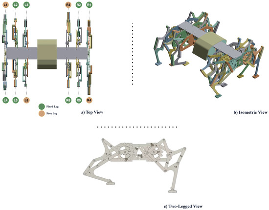
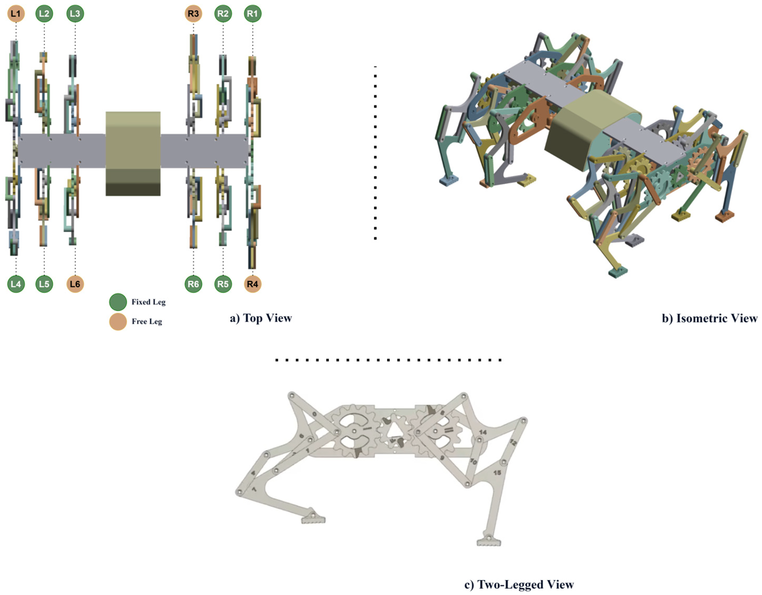
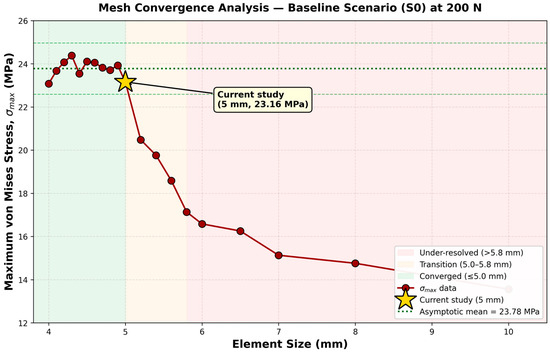
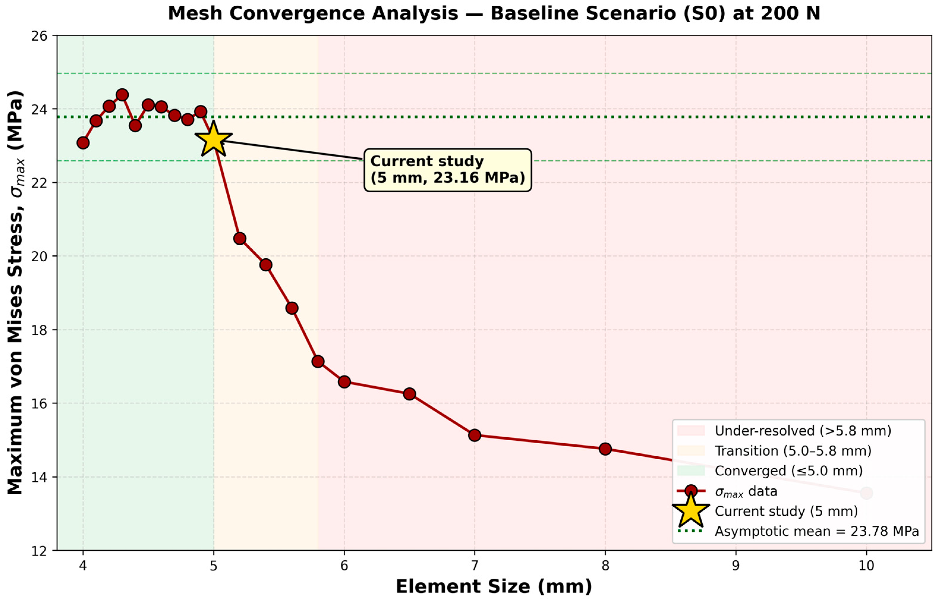
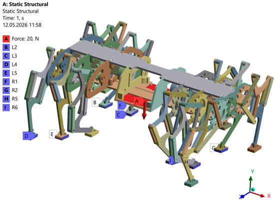
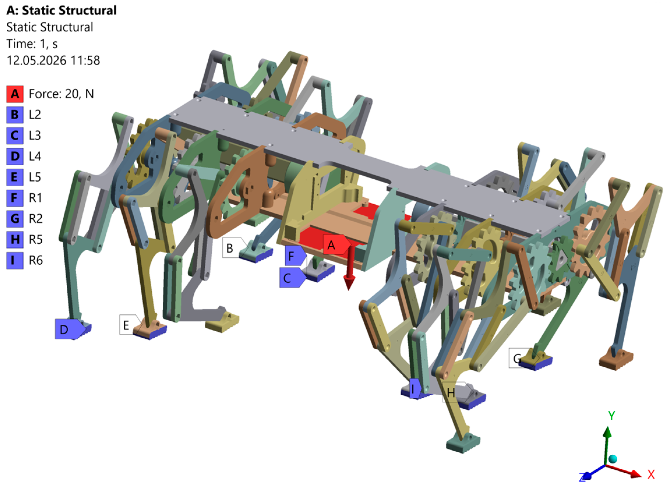
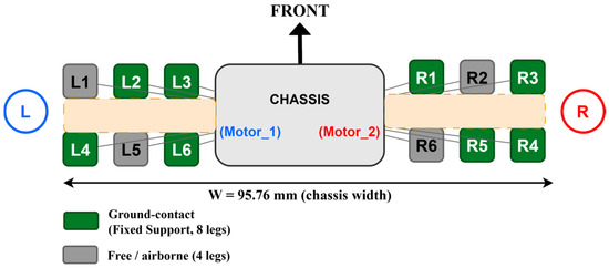
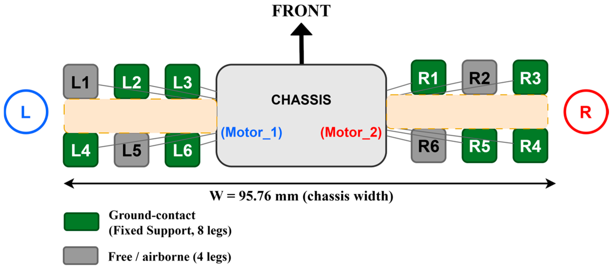
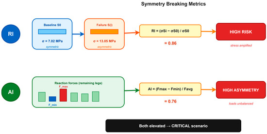
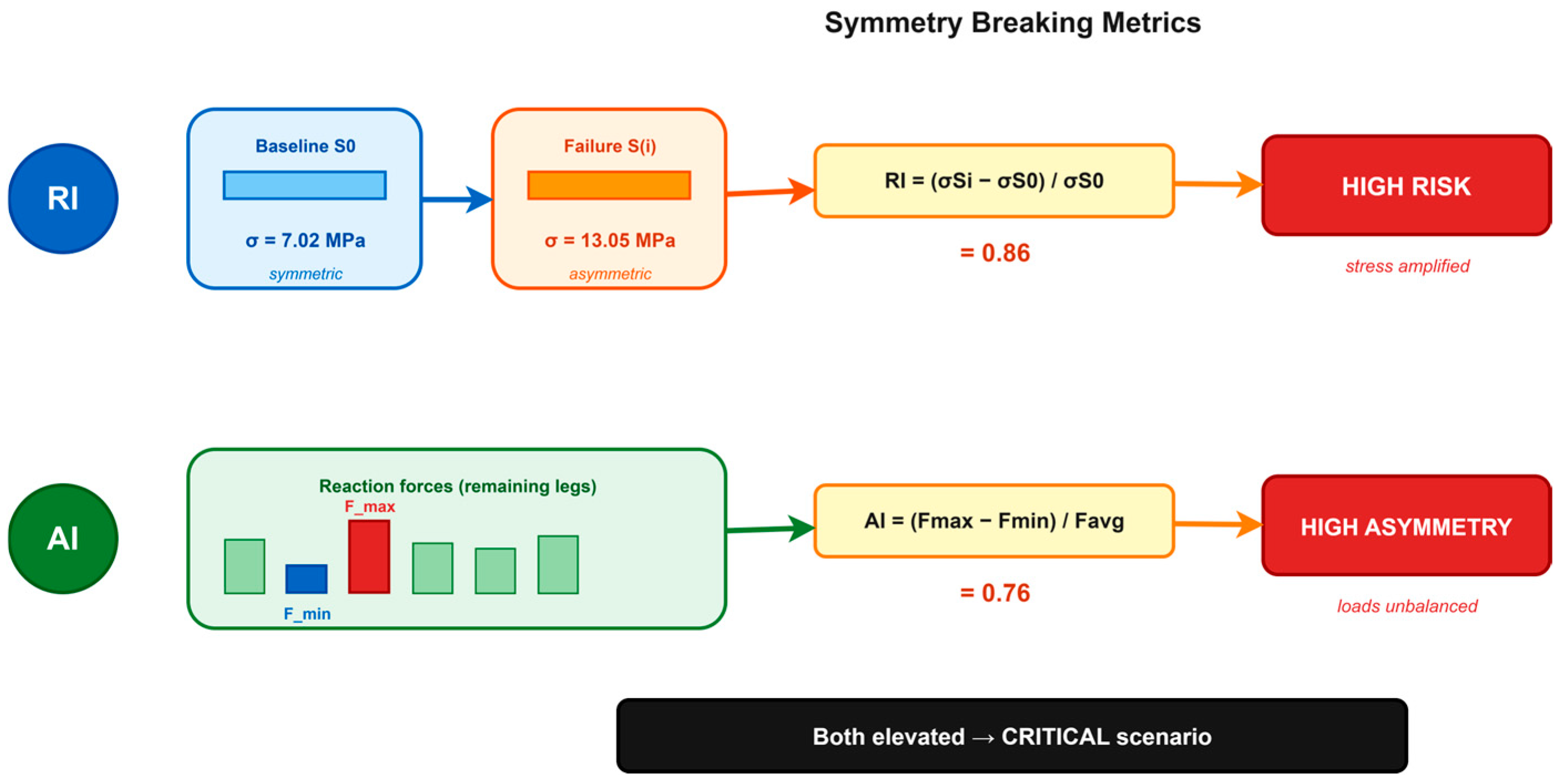
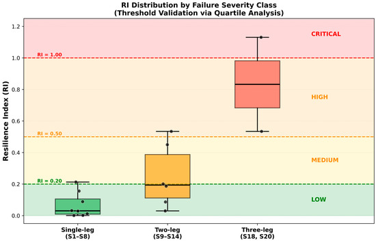
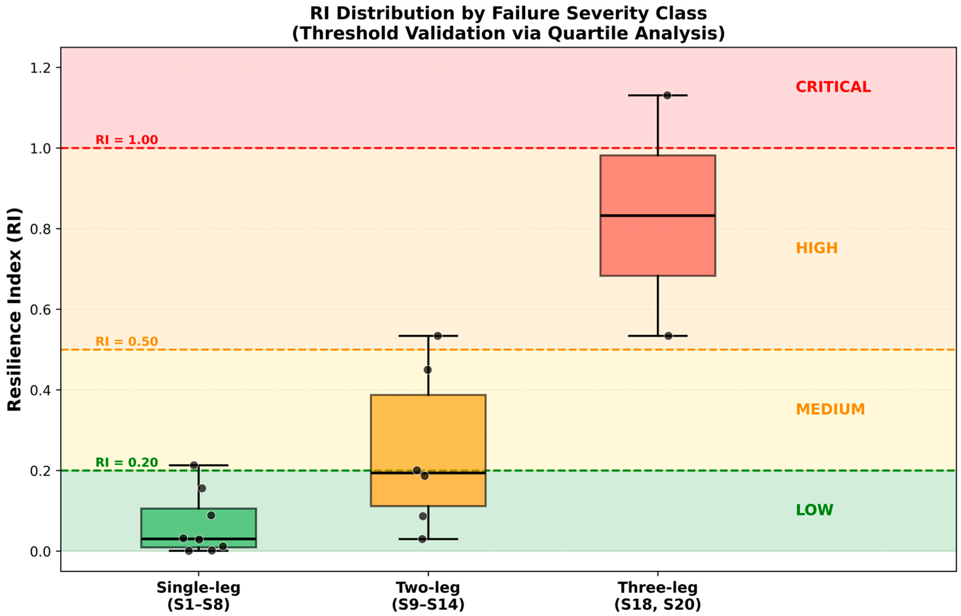
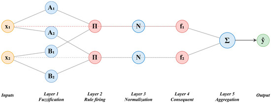
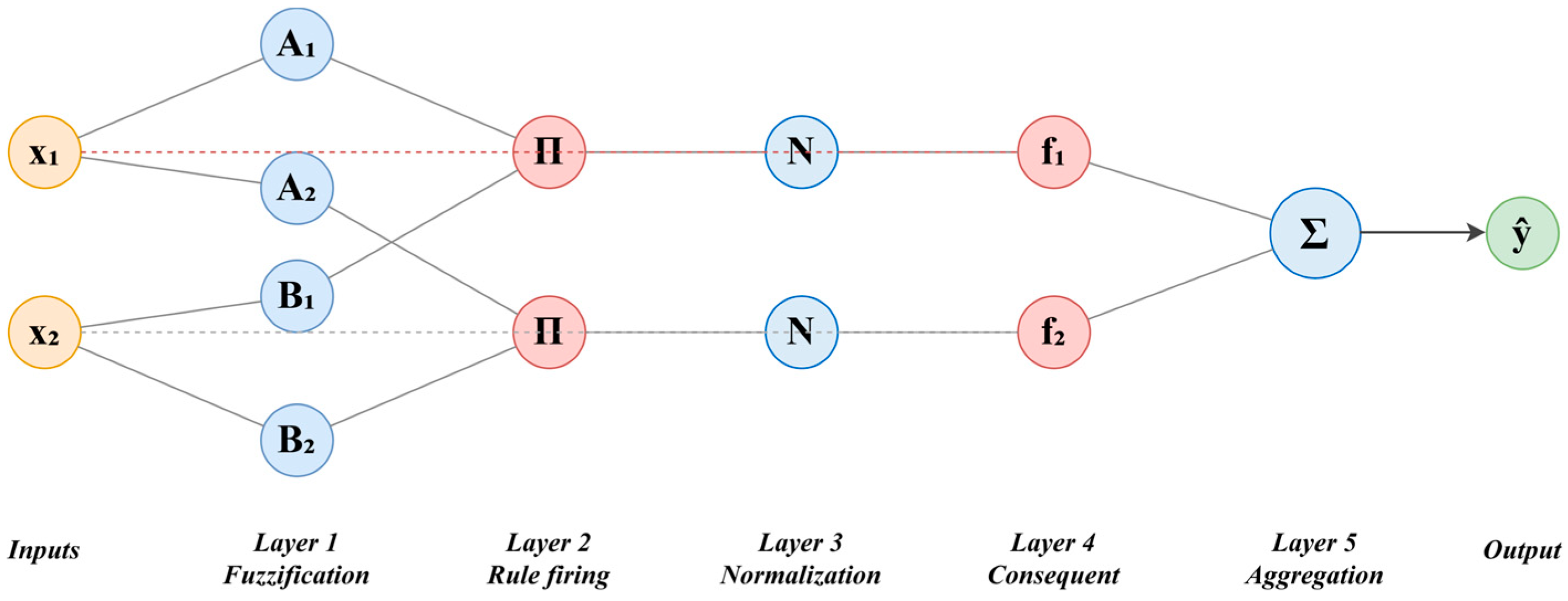
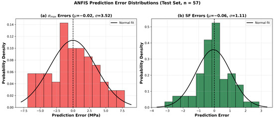
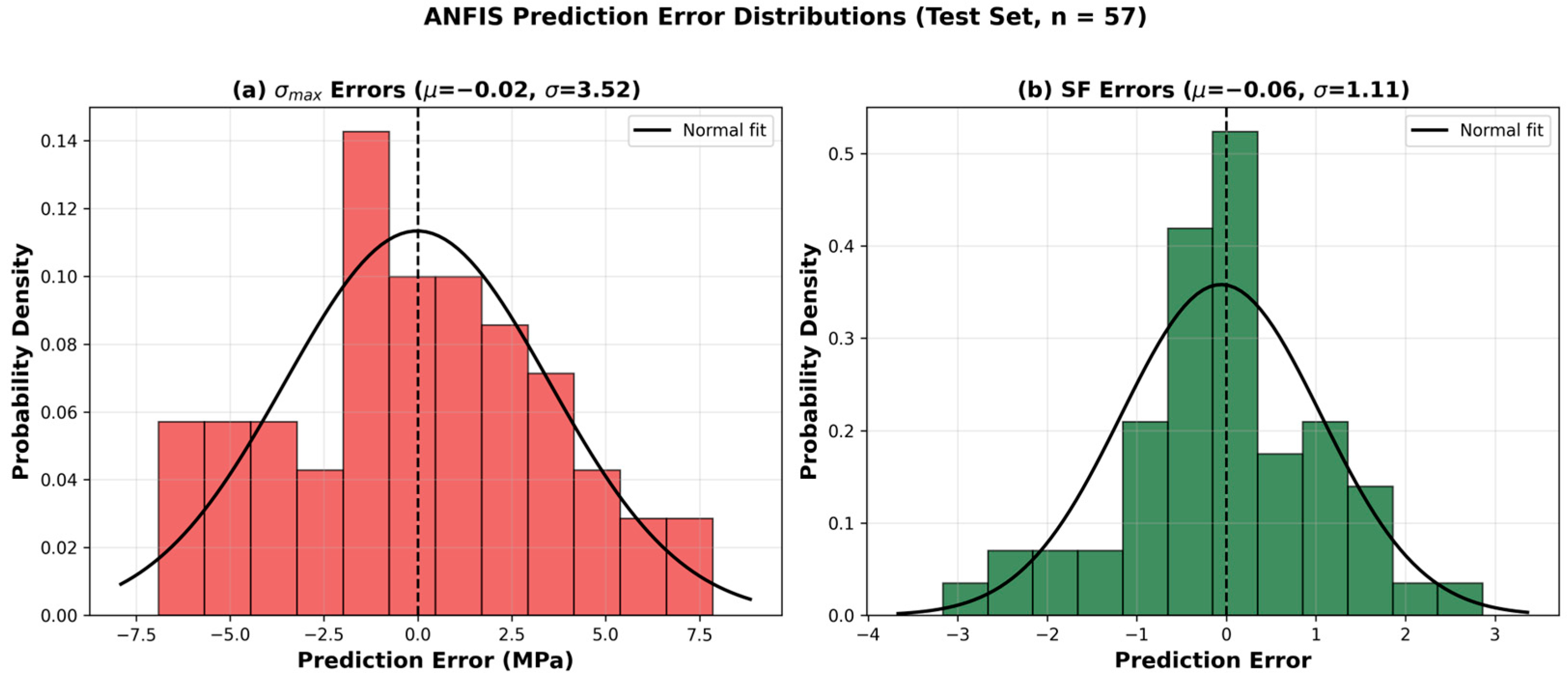
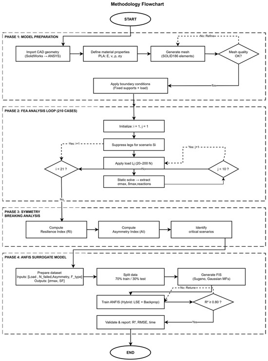
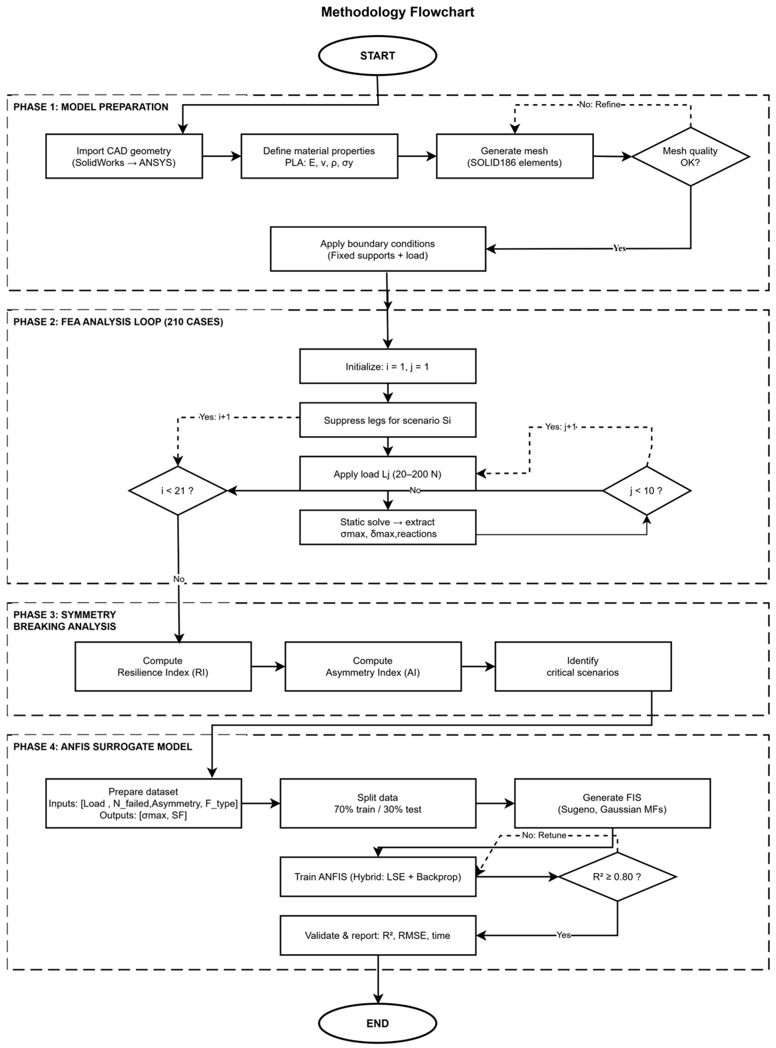
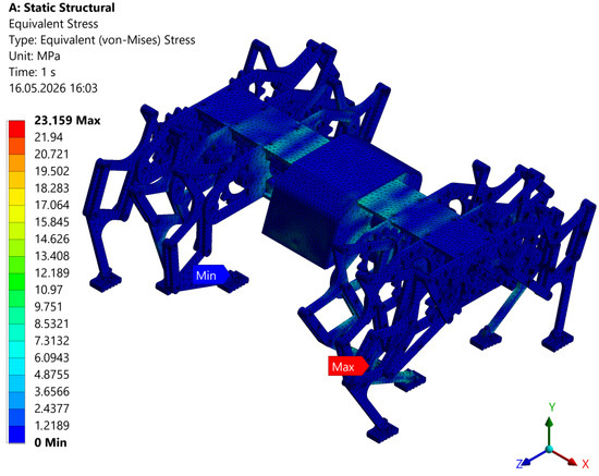
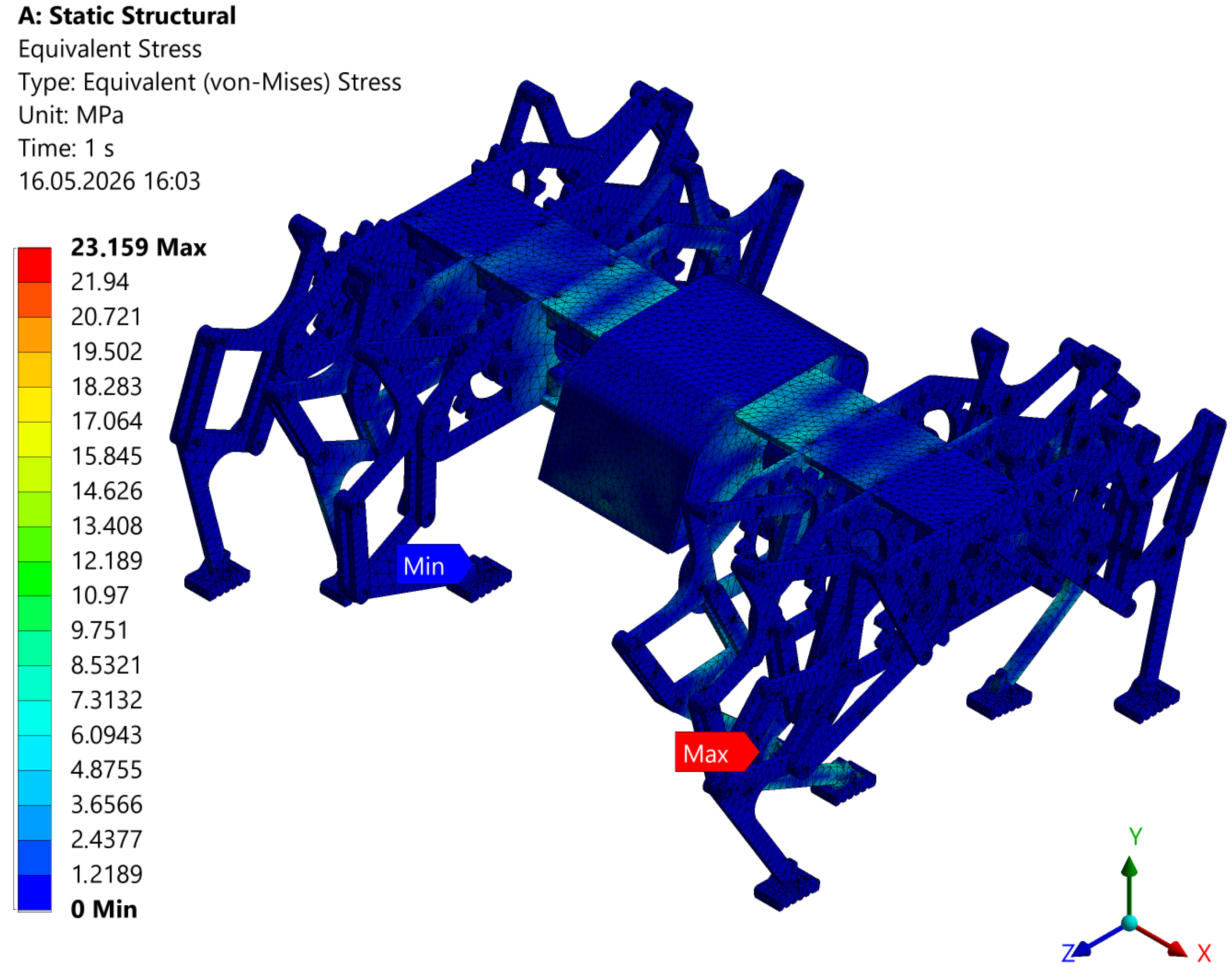
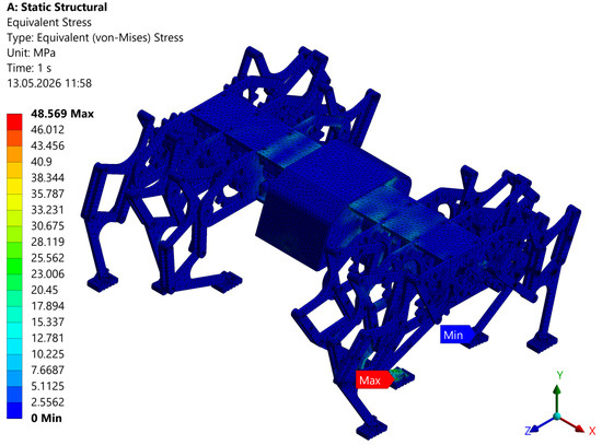
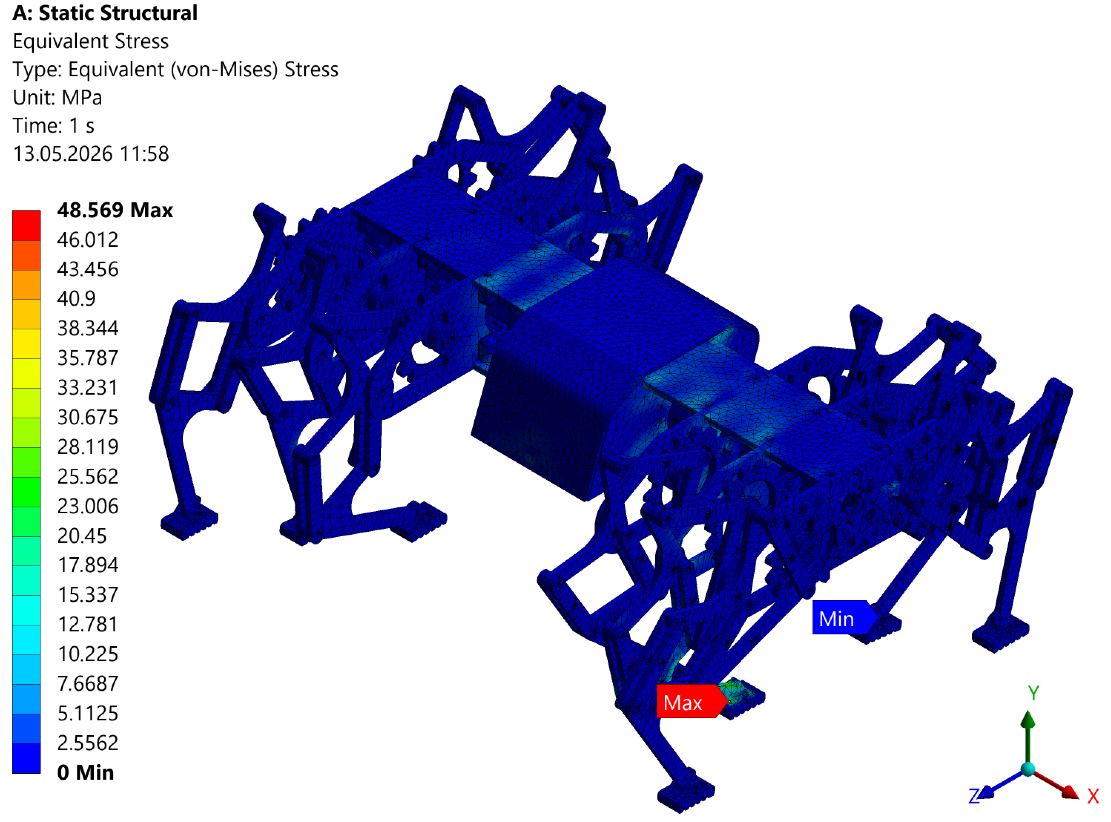
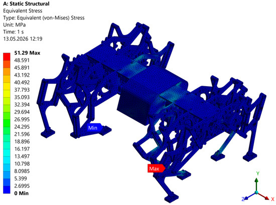
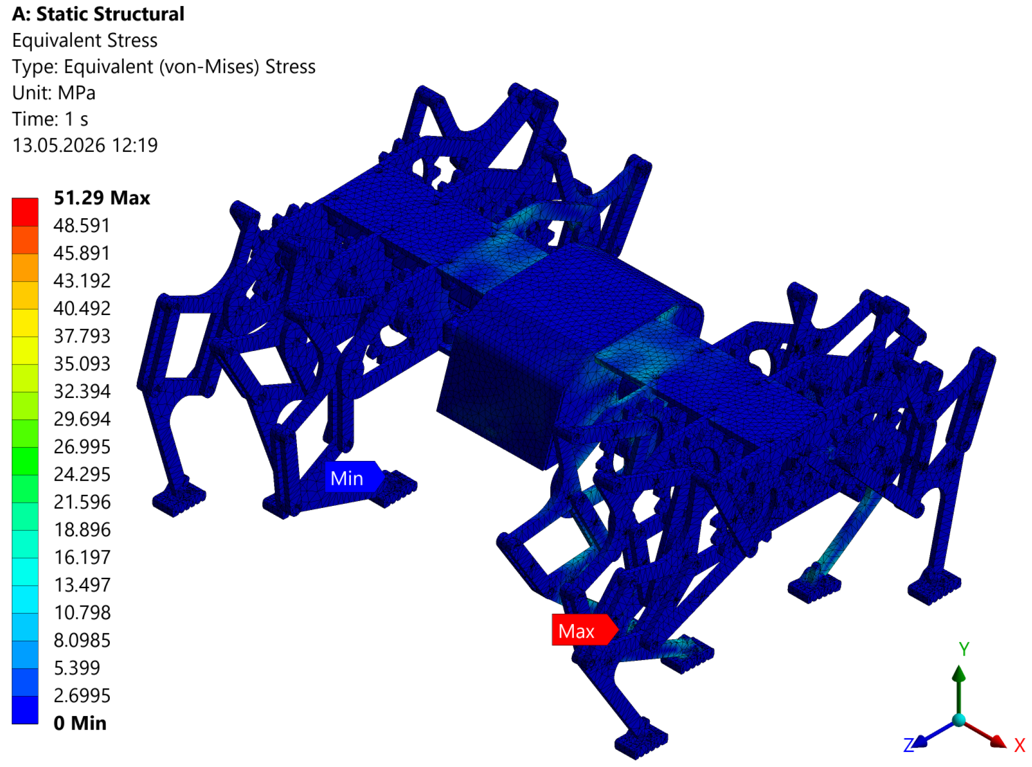
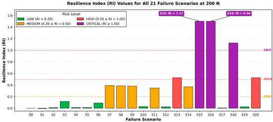
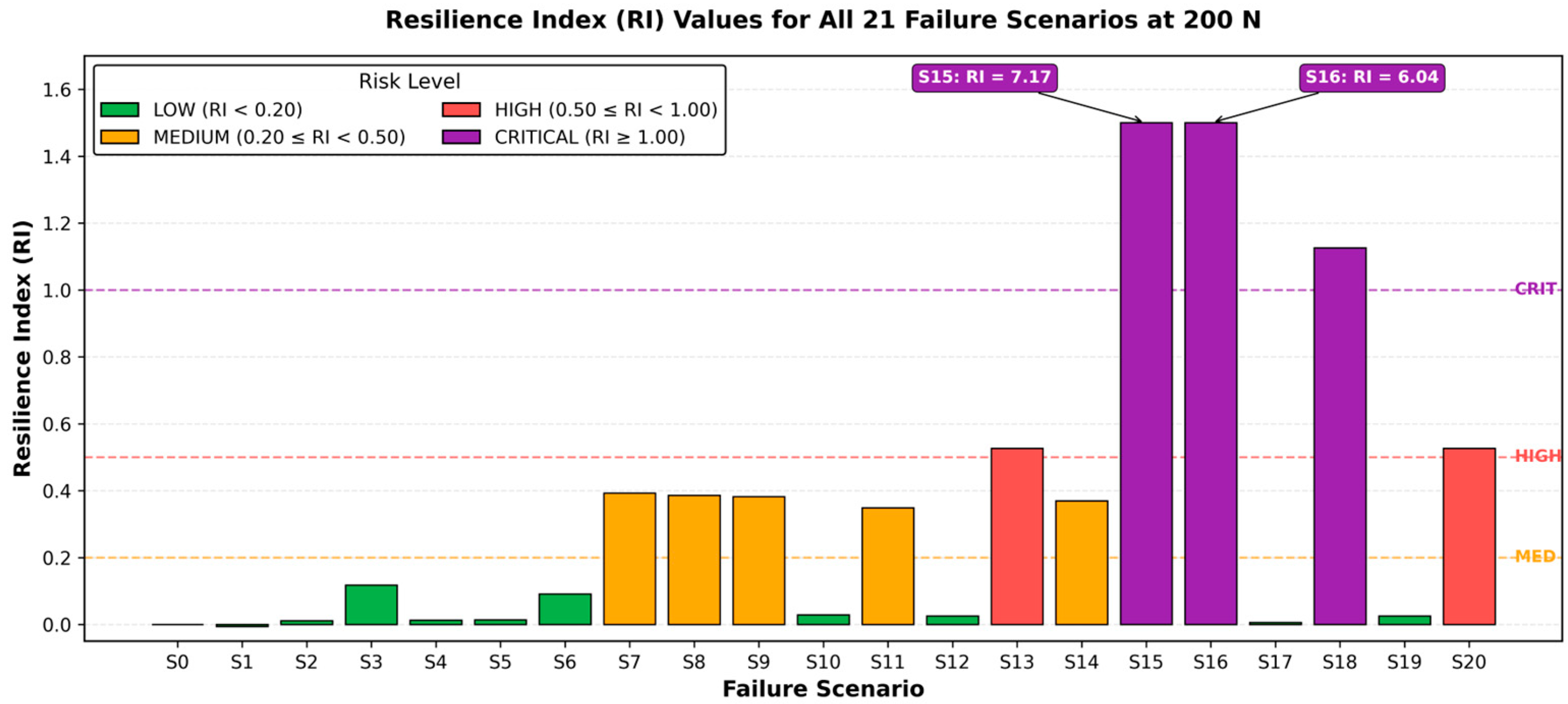
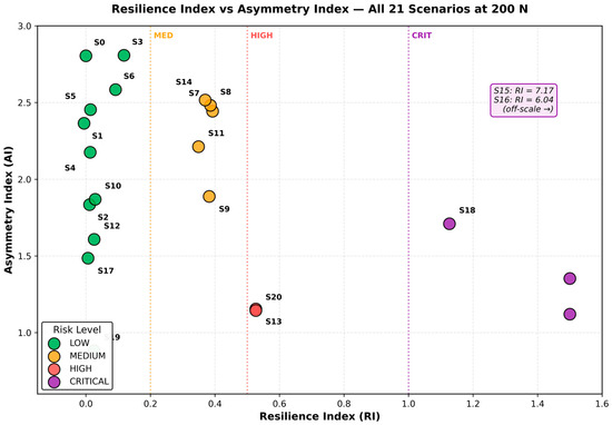
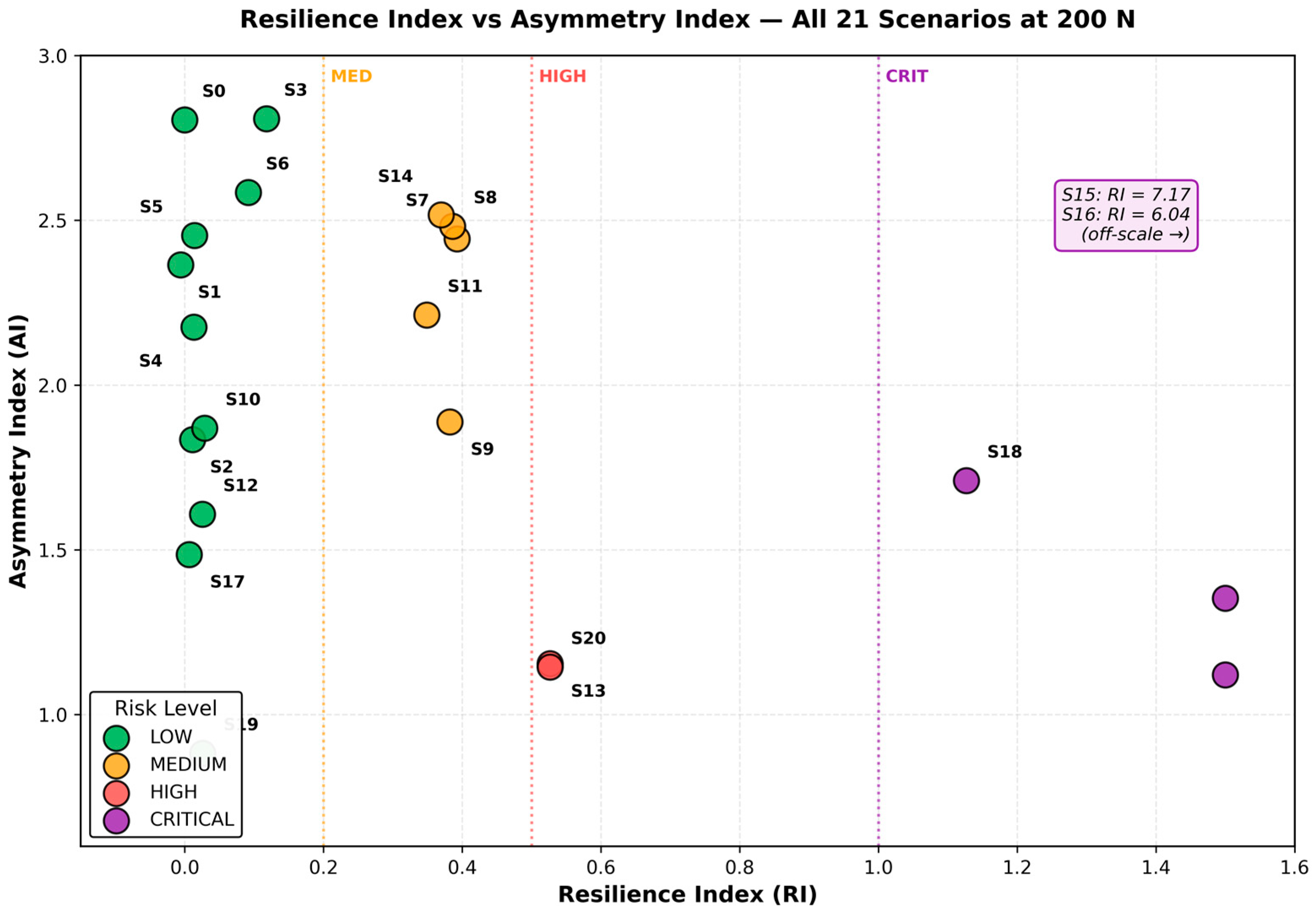
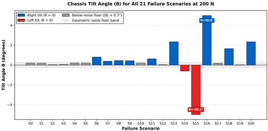
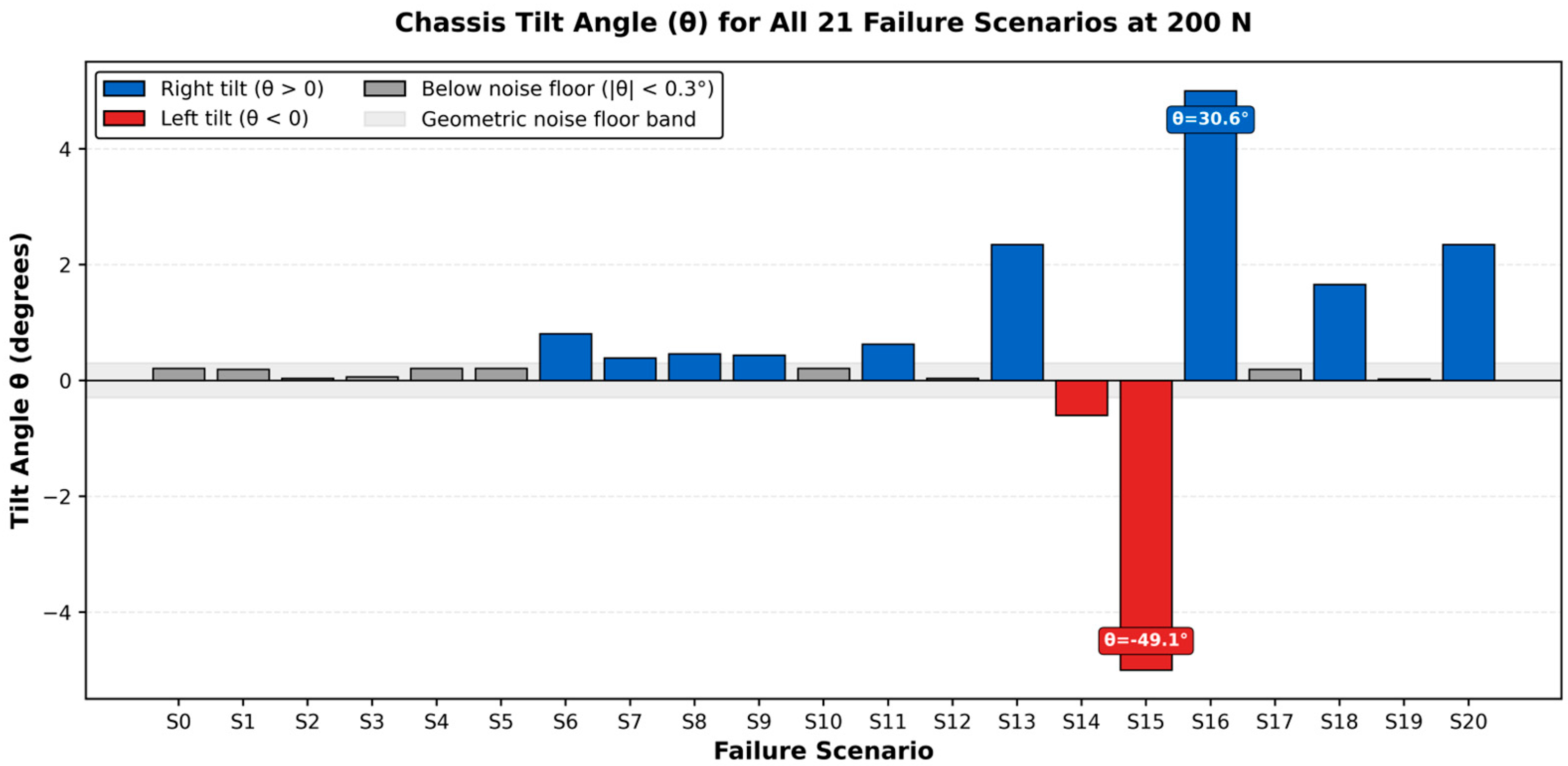
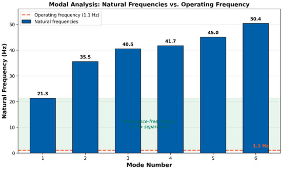
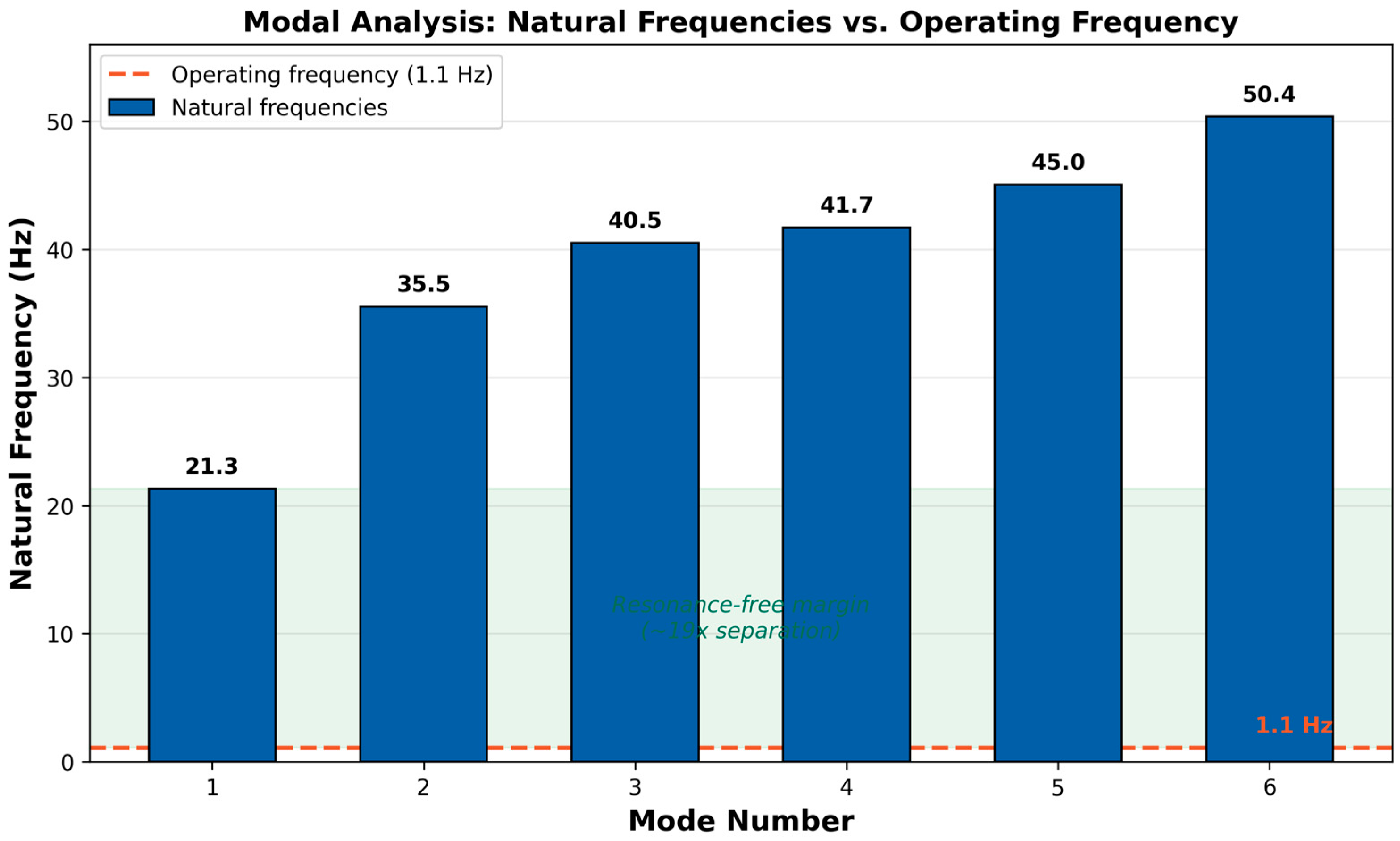
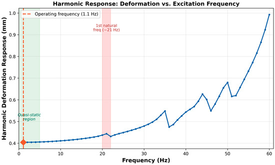
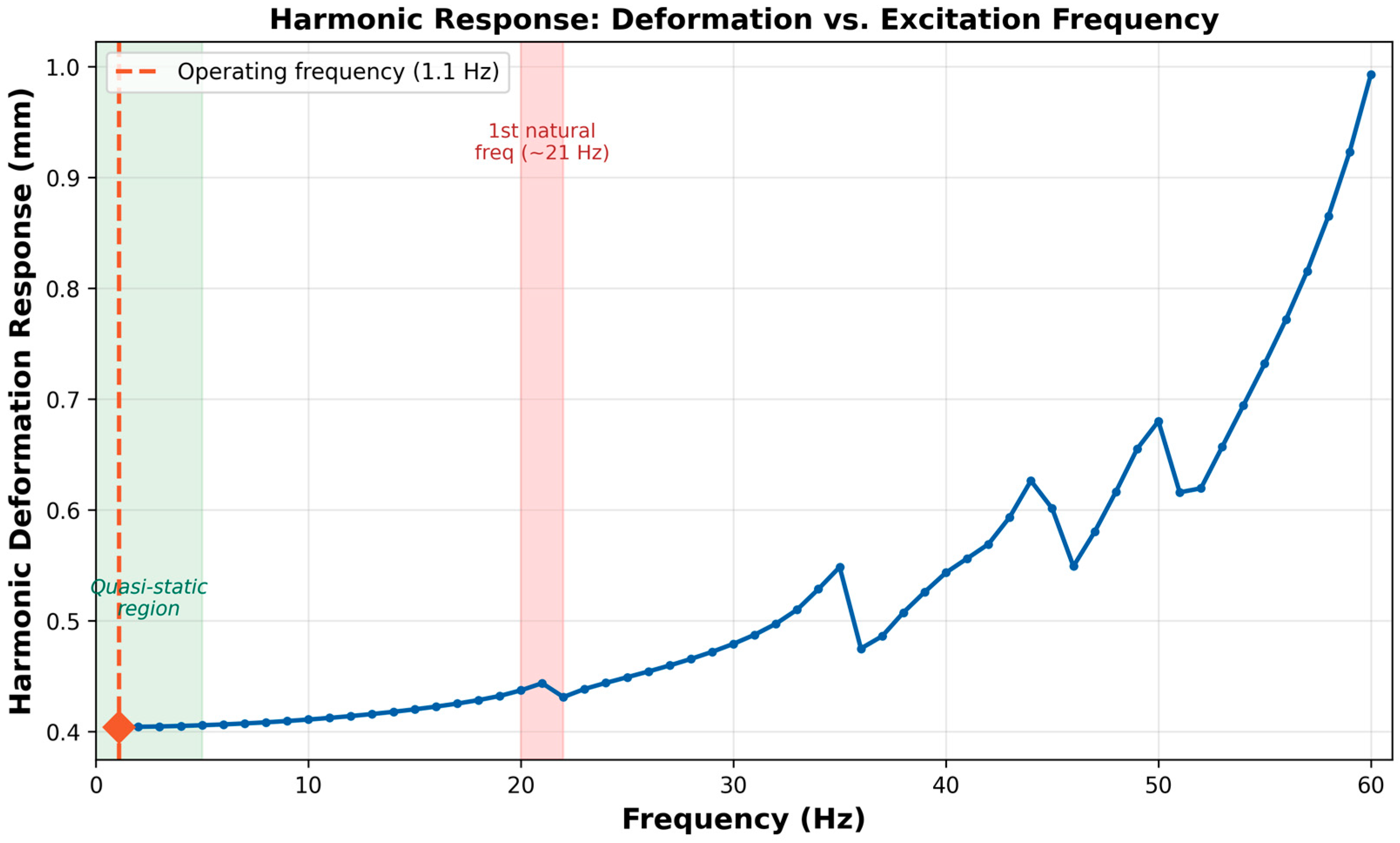
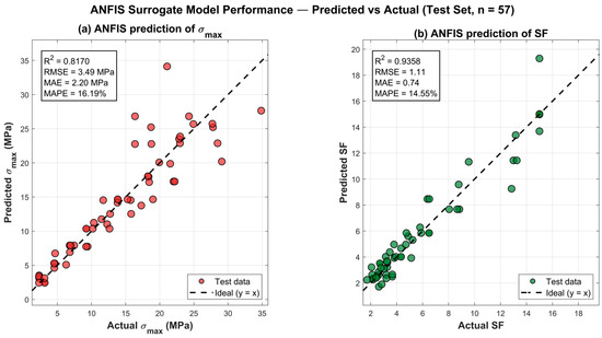
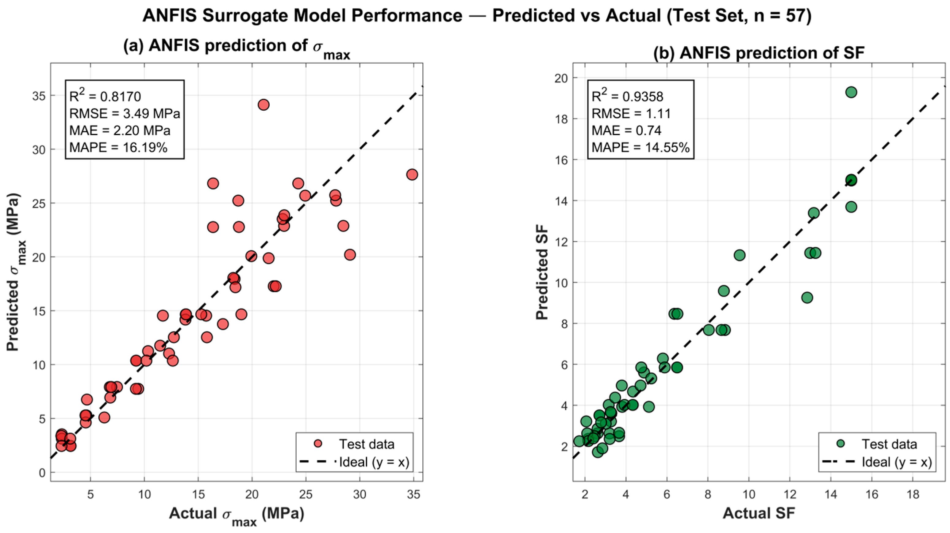
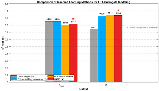
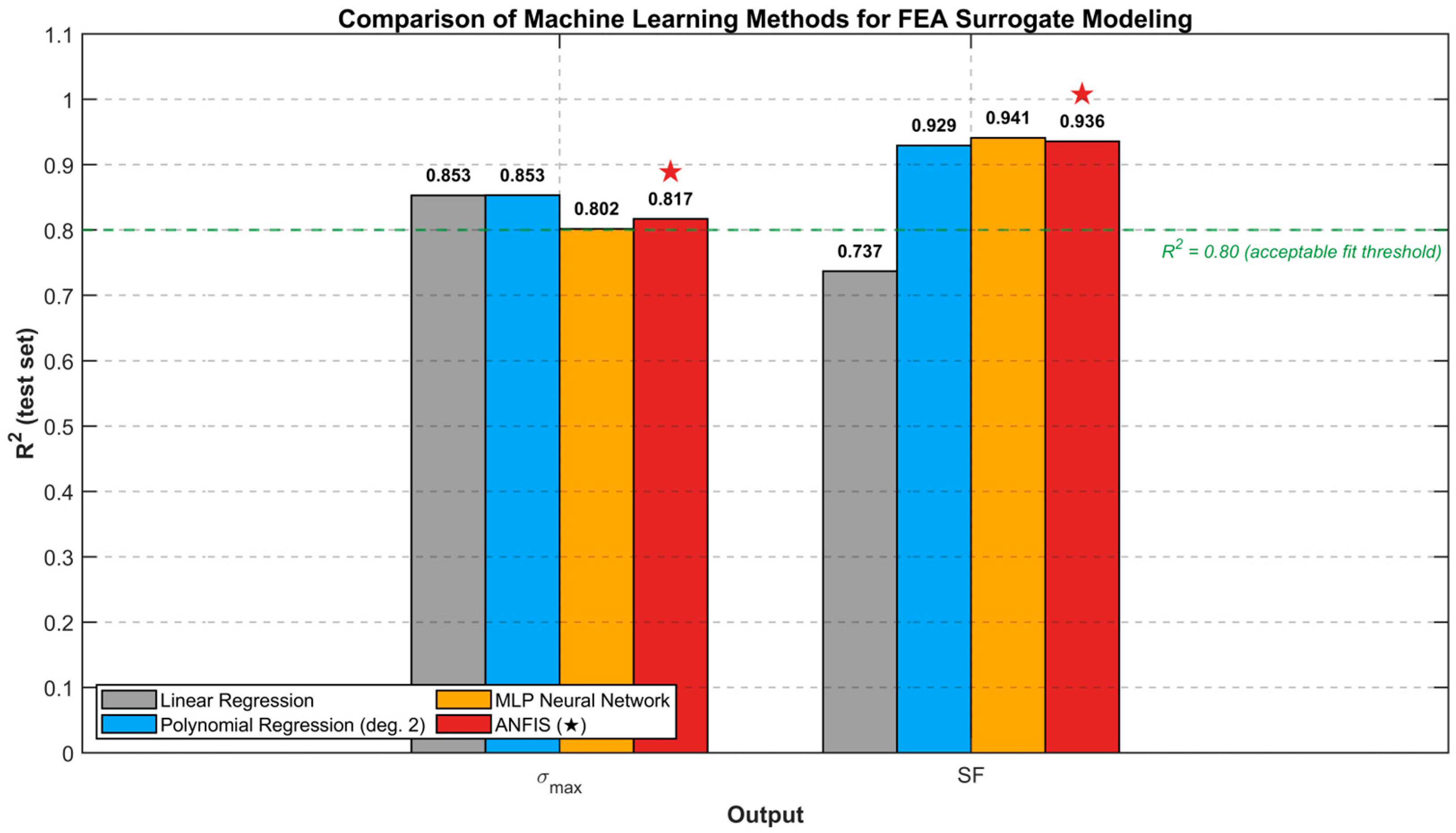
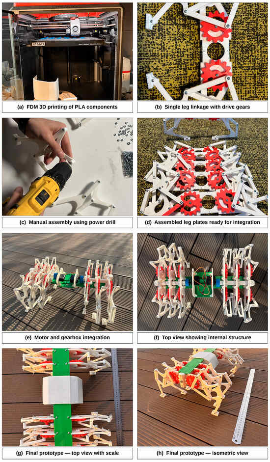
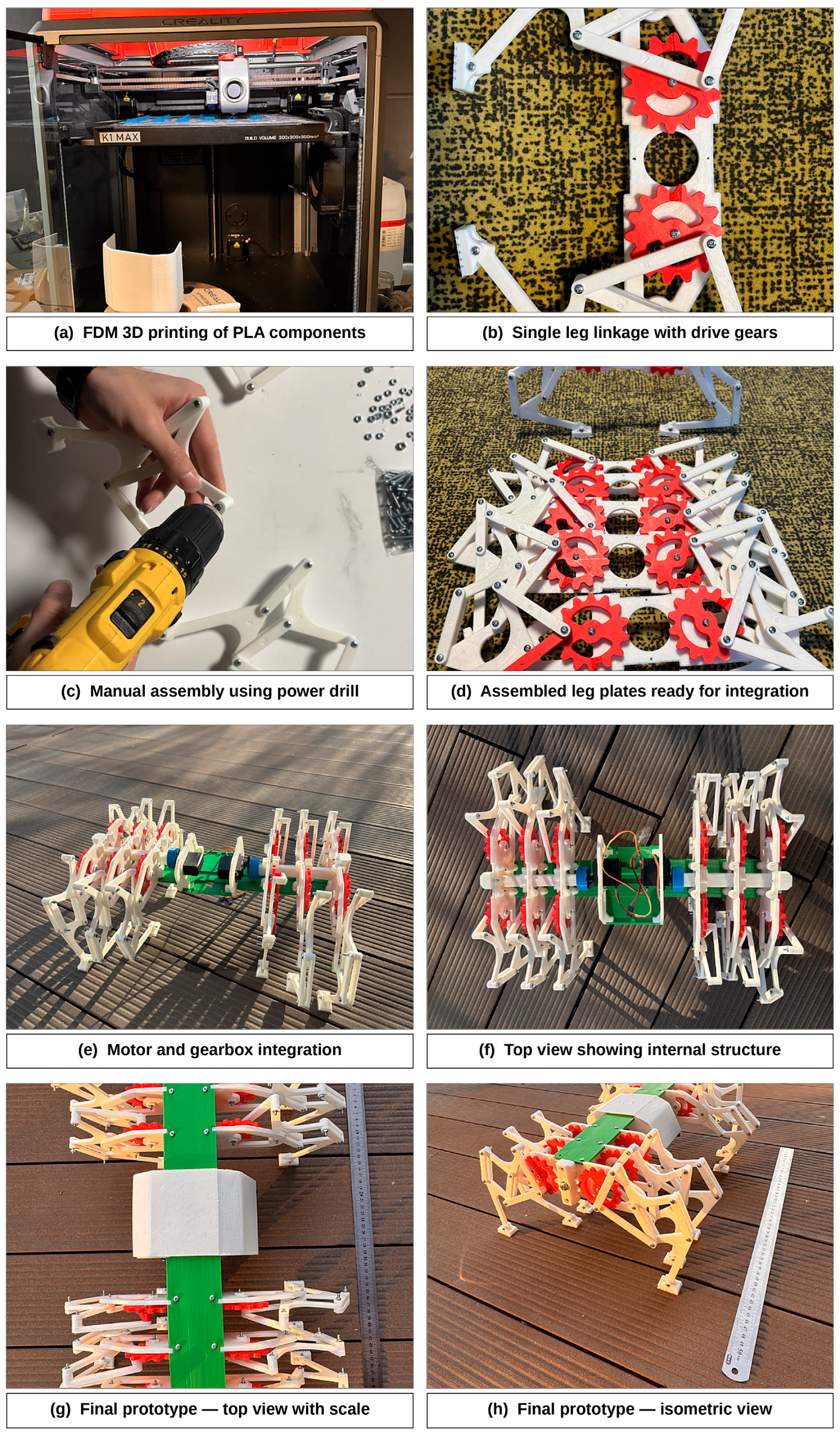

Disclaimer/Publisher’s Note: The statements, opinions and data contained in all publications are solely those of the individual author(s) and contributor(s) and not of MDPI and/or the editor(s). MDPI and/or the editor(s) disclaim responsibility for any injury to people or property resulting from any ideas, methods, instructions or products referred to in the content. |
© 2026 by the authors. Licensee MDPI, Basel, Switzerland. This article is an open access article distributed under the terms and conditions of the Creative Commons Attribution (CC BY) license.