


Abstract
This paper proposes a superelliptic dual quaternion framework that extends classical dual quaternion kinematics by replacing the Euclidean metric structure with a Gielis-formula-induced superelliptic inner product and its associated vector product. Within the resulting space , superelliptic dual numbers, dual vectors, and an E-Study-type correspondence between unit dual vectors and directed superelliptic lines are established, yielding an algebraic model adapted to non-Euclidean geometric profiles. In contrast to the standard Euclidean dual quaternion formalism, where rotations, translations, and screw motions are governed by the ordinary inner product of , the present formulation encodes these motions relative to a parameter-dependent superelliptic geometry determined by Gielis’ superformula. This distinction enables the kinematic description of motions associated with superelliptic axes and trajectories that cannot be represented naturally within the classical Euclidean setting. A superelliptic screw motion theorem is obtained, showing that a unit superelliptic dual quaternion generates simultaneous rotation about and translation along a common superelliptic axis. The framework offers a compact mathematical basis for advanced rigid-body modeling in robotics and geometric design. The proposed framework represents rotation, translation, and screw displacement by a single unit superelliptic dual quaternion, providing a compact basis for shape-dependent rigid-body modeling in robotics and geometric design.
MSC:
11R52; 70B10; 39B42; 65F60; 53A05; 70E1
1. Introduction
Superellipses are getting more and more attention in modern research because they are very good at describing and parameterizing things. In three-dimensional modeling, they offer a versatile structure for depicting shapes with greater realism and precision than numerous traditional geometric forms. Superelliptic representations are used in many fields, such as computer engineering, physics, biology, robotics, and geometry. Previous research has shown that many natural patterns and biological structures, especially those found in plants and animals, are more accurately represented by superelliptic curves than by circles or standard ellipses. Superellipses and their generalizations have gained prominence in both theoretical and applied research due to their geometric versatility, concise mathematical representation, and efficacy in modeling intricate shapes.
G. Lamé generalized the equations of the circle and ellipse so as to include squares, rectangles, rhombuses, and astroids within a single mathematical formulation [1]. This formulation later inspired Piet Hein, who introduced the term superellipse for a curve lying geometrically between a rectangle and a circle [2]. One of the earliest engineering applications of the superellipse was reported by Flanagan and Hefner in 1967 in the design of aircraft fuselage cross-sections [3]. Thereafter, Gridgeman analyzed Lamé curves for various parameter values and alternative forms of the general superellipse equation [4], while Matsuura investigated how the maximum curvature of Lamé curves varies with the superellipse parameters and characterized the corresponding extremal conditions [5].
Barr introduced superquadrics as a three-dimensional extension of superelliptic geometry, defined by parameters that govern edges, corners, and surface shape [6]. This advancement offered a versatile mathematical framework for geometric modeling that extends beyond traditional quadric surfaces. Later, Franklin and Barr suggested a different way to use parameters that made it easier to find points on superquadric surfaces than traditional methods [7]. Pentland advanced this research trajectory by presenting deformed superquadrics as a substitute for generalized cylinders and by illustrating their efficacy in modeling natural shapes for computer vision [8]. Gielis proposed the superformula as a comprehensive mathematical expression that can encapsulate a wide range of natural and abstract forms beyond those delineated by classical Euclidean geometry [9]. Additionally, optimization-based research has demonstrated that superelliptic models can produce superior volumetric object representations compared to traditional ellipses [10]. Using the superformula, Tavkhelidze et al. looked into the geometric shapes and particle-like forms that come from cutting Möbius–Listing bodies [11]. Lamé–Gielis curves, which are a generalization of classical Lamé curves, provide a precise mathematical way to describe natural shapes and how they grow both inside and outside of themselves [12]. Additionally, models based on superquadrics and superellipses have resulted in effective methods for geometric representation and shape compression in fields like computer graphics and digital modeling [13].
Hamilton introduced quaternions as a four-dimensional extension of complex numbers, offering a robust algebraic framework for rotations in three-dimensional space [14]. After this, Clifford introduced dual numbers, which later became very important in geometric and kinematic formulations [15]. Several authors, such as Cayley, Kelland, and Hardy [16,17,18], later built on the theory of quaternions. Quaternions have practical uses as well as theoretical importance. For example, they can be used to animate rotations on the unit sphere and show random spherical curves [19]. The study further developed this framework via the transformation named after him, employing dual numbers and dual vectors to depict directed lines [20]. Later, McAulay combined dual numbers and quaternions, which led to the creation of dual quaternions [21]. These improvements laid the groundwork for modern geometric kinematics in math. Quaternion algebra has been employed to delineate rotation operators for matrices and has achieved extensive technological applications [22]; moreover, quaternion-based methodologies have demonstrated particular efficacy for successive rotations in inertial navigation [23]. Screw theory, which Sir Robert Stawell Ball introduced, has become very important for studying robot kinematics and rigid-body dynamics [24].
Dual quaternion methods have developed into a powerful framework for the representation and analysis of rigid-body motion, with applications spanning robotics, estimation, control, and geometric modeling. A formulation for solving the kinematic problems of multiarm robot systems within the screw-theoretic setting by means of quaternion algebra was presented in [25]. This line of research was subsequently extended to three-dimensional kinematics and its applications in neuroscience through a dual-quaternion formalism in [26], while a unified representation of points, lines, screws, and planes in dual quaternion kinematics was established in [27]. Building on this geometric and algebraic foundation, unit dual quaternions were employed for the kinematic modeling and control of robot arms in [28], and later advanced toward robust and efficient formulations of forward, differential, and inverse kinematics in [29]. Generalized representations of rigid-body kinematics via hyper dual quaternions were reported in [30], followed by motion-control strategies based on kinematic screws and dual quaternions in [31]. Interpolation and motion generation were addressed through dual-quaternion interpolation in [32] and real-time motion planning based on cascade dual-quaternion screw-geometry MPC in [33]. A comprehensive review of dual quaternion applications was provided in [34], confirming the growing relevance of this formalism across disciplines. More recent studies have focused on rigid-body motion operations and hand–eye calibration [35], RRT*-based path planning for satellite rendezvous and docking [36], spacecraft screw-motion tracking [37]. Beyond classical Euclidean rigid-body motion, this research direction has also expanded toward shape-dependent generalized geometries through the introduction of superelliptic motion and superelliptic quaternions via the Gielis formula in [38], and further through superquadric motion and superquadric hyperbolic split quaternion algebra in [39].
Although the present study is motivated by our previous works on superelliptic motion and superelliptic quaternions via the Gielis formula [38] and on superquadric motion with hyperbolic split quaternion algebra [39], it differs from them by introducing a dual-quaternion-based kinematic structure. While ordinary superelliptic quaternions mainly describe rotational behavior in the Gielis-formula-induced metric, a superelliptic dual quaternion , with , simultaneously encodes rotation, translation, and line-moment information. Here, s represents the superelliptic rotational part, whereas represents the translational or moment component of a directed superelliptic line. Thus, the present framework extends previous shape-dependent quaternionic models to a screw-theoretic setting through the superelliptic E-Study correspondence and the superelliptic screw motion theorem. This paper is devoted to the study of superellipses, superelliptic dual quaternions, and superelliptic screw motion, motivated by the occurrence of superelliptic forms in natural and man-made structures. As three-dimensional generalizations of superellipses, superquadrics provide a more realistic geometric setting for the modeling of complex shapes and motions.
The remainder of the paper is organized as follows. Section 1 outlines the historical background and main applications of superellipses and quaternions. Section 2 introduces the basic concepts and notation. Section 3 defines superelliptic dual numbers and vectors. Section 4 develops superelliptic quaternions and the main theorem on superelliptic screw motion. The final section visualizes the proposed superelliptic screw motion through Gielis-formula-based curves generated by MATLAB R2024a.
2. Basic Concepts and Notions
The Gielis formula, also known as the superformula, is a basic idea behind this study. This formulation derives from the prior contributions of Gabriel Lamé, who generalized the equations of the circle and ellipse to include squares, rectangles, parallelograms, and astroids within a singular mathematical expression [1]. The Lamé curve that goes with it can be written as
where a, b, and n are all positive numbers. Accordingly, Lamé curves have become a significant subject in geometric analysis. Previous studies have shown that the parameters in the Lamé curve equation determine the deformation between ellipse-like and rectangle-like geometries [40]. The polar form of the Lamé curve is given by
In the 1990s, Johan Gielis introduced the following generalization of the Lamé curve:
He referred to this expression as the superformula, since it extends the classical Lamé equation to a broader parametric family of curves. Here, , the real parameters m, a, b, , , and , which collectively determine the rotational symmetry, local curvature behavior, and overall geometric structure of the resulting curve, under the assumption that , , and . By varying these parameters, the superformula provides a unified mathematical framework for representing a wide range of natural and abstract forms beyond standard Euclidean curve families [2,9,13]. Gielis referred to these parameter-dependent forms as supershapes. In the related literature, the terms superellipse, Gielis formula, and Gielis curve are also used in closely related settings. To introduce the underlying geometry of the proposed framework, we equip with a symmetric positive-definite bilinear form. For and in , we define
where
and for . The parameters m, a, b, , , and each contribute fundamentally to the geometric formation of the superelliptic structure. The scaling coefficients a, b, and regulate the directional dilation and anisotropic stretching of the geometry along the coordinate axes, whereas the parameter m prescribes the rotational periodicity and symmetry order of the generated profile. In contrast, the exponents , , and control the local and global morphological behavior of the shape by influencing curvature concentration, edge sharpness, and smoothness transitions. In particular, smaller values of tend to generate angular or corner-type formations, while larger values produce progressively smoother and more rounded geometric configurations. It is also essential to emphasize the geometric character of the superelliptic inner product introduced in this setting. Although the formulation involves the direction-dependent radial function , this dependence enters the metric structure only through a smooth conformal-type modulation of the classical Euclidean inner product. Consequently, at every point of the underlying manifold, the associated bilinear form preserves symmetry, bilinearity, and positive definiteness on the tangent space. Therefore, the induced geometric framework remains intrinsically Riemannian. The role of the superelliptic factor is not to alter the metric category itself, but rather to introduce an anisotropic and direction-sensitive scaling mechanism that enriches the geometric behavior of the space while maintaining the fundamental properties of a Riemannian metric tensor. When and , the metric tensor reduces to the Euclidean identity matrix, and the superelliptic dual quaternion model reduces to the classical dual quaternion kinematics. Vectors and will be referred to as superelliptic vectors. The bilinear form is called the superelliptic inner product. The space endowed with this inner product is called the superelliptic 3-space and is denoted by
Moreover, the superelliptic inner product can be expressed in matrix form as
where the associated matrix G is given by
The length of a superelliptic vector associated with the superelliptic inner product is given by
In , any two superelliptic vectors and are called superelliptic orthogonal if and only if Additionally, if the superelliptic norm of each superelliptic vector is equal to 1, then these vectors are called superelliptic orthonormal vectors. Let us denote the standard basis of Euclidean 3-space as . Then, the base vectors of can be denoted as and satisfy
and any vector can be written in the following form:
Let and be two non-zero superelliptic vectors; the cosine function of the angle between them
where is in agreement with the angular parametric equations of a superellipse or a superellipsoid. The superelliptic cross product of two vectors is given by
where and are positive real numbers (see [38,39] for details).
3. Superelliptic Dual Numbers and Vectors
In this section, we will define dual numbers and dual vectors defined in relation to the superelliptic inner product, which we will use to describe superelliptic E-Study transformation, dual quaternions and screw motion.
3.1. Superelliptic Dual Numbers
Definition 1.
A dual number can be denoted as and the set of the dual numbers is given by
For any superelliptic dual number , the real part and dual part are denoted, respectively, as , , .
In , for and
addition operation
is a ring with unity and commutativity with respect to the multiplication operation. In the set of superelliptic dual numbers, the identity element with respect to addition is , and for every
due to the superelliptic dual number is a unit element with respect to multiplication. The conjugate of any superelliptic dual number is denoted as
Definition 2.
For any vectors we define the superelliptic inner product as
Definition 3.
For any the superelliptic norm is calculated as follows:
3.2. Superelliptic Dual Vectors
Definition 4.
Let us define the set as follows:
Let us take and . Then, we can write the following equations:
and
According to these operations, the set is a module on the ring of superelliptic dual numbers. Each element of the module is called a superelliptic dual vector.
Theorem 1.
Each superelliptic dual vector can be written in the form , here .
Proof.
By definition, where each component is a superelliptic dual number of the form Let Then
Separating the real and dual parts component-wise, we obtain
Define
and
Hence,
Therefore, every superelliptic dual vector
can be expressed in the form
□
Definition 5.
For any two dual vectors , the superelliptic dual inner product is defined as follows:
Definition 6.
For any dual vector the superelliptic norm can be defined as follows:
If we have and , then the dual vector is called a unit superelliptic dual vector.
Definition 7.
On module the set
is called unit dual superellipsoid.
Definition 8.
Directed superelliptic lines have a specific direction and orientation and are expressed as follows:
Namely, it can be defined as the line that passes through the superelliptic point and has the superelliptic direction vector .
Theorem 2 (Superelliptic E-study transformation).
The points of the dual superellipsoid correspond to directed superelliptic lines in the space in a one-to-one connection. In other words, a directed superelliptic line in the space is equivalent to each unit superelliptic dual vector.
Proof.
Let P be a fixed reference point in . We first show that every directed superelliptic line determines a unit superelliptic dual vector. Let l be a directed superelliptic line with unit direction vector , that is,
Choose a point , and put
The moment vector of l with respect to P is defined by
We claim that does not depend on the choice of the point on the line. Indeed, if is another point and
then, since and lie on the same directed line, there exists such that
Therefore,
Hence,
Thus, the vector is well defined. Since , the vector is superelliptically orthogonal to . Hence,
Together with , this gives
Therefore, every directed superelliptic line determines a unit superelliptic dual vector. Conversely, let
Then
We shall construct a directed superelliptic line whose direction vector is and whose moment vector is . Consider the superelliptic orthogonal complement of ,
Define the linear map
If , then
Thus, is parallel to . On the other hand, , so
Since , the only vector which is both parallel and orthogonal to is the zero vector. Hence,
Therefore, is injective. Since is two-dimensional, is also surjective. Because , there exists a unique such that
Now let C be the point satisfying
Define to be the directed superelliptic line passing through C with direction vector . In parametric form, this line is
Equivalently, in the coordinate notation of , it can be written as
By construction, its moment vector is
Therefore, the directed superelliptic line corresponds to the unit dual vector
It remains to prove uniqueness. Suppose that the same unit superelliptic dual vector
corresponds to two directed superelliptic lines and . Let and be the closest points of and to P, respectively, and put
Since both lines correspond to the same U, we have
Subtracting these equations gives
Hence, is parallel to . On the other hand, since and are the closest points to P, we have
Therefore,
Thus, is both parallel and superelliptic orthogonal to . Since , this implies
Hence,
The two directed lines have the same direction vector and pass through the same closest point . Consequently,
Thus, each directed superelliptic line determines exactly one unit superelliptic dual vector, and each unit superelliptic dual vector determines exactly one directed superelliptic line. Hence, the correspondence is bijective. □
The following example illustrates the practical role of the superelliptic E-Study correspondence. In particular, it shows how a given unit superelliptic dual vector determines a directed superelliptic line explicitly.
Example 1.
Let us find the directed superelliptic line corresponding to the unit superelliptic dual vector , for , , and . In Study’s mapping, a point on the line is obtained from
Hence, the line passes through the point
with direction vector
Therefore, the parametric equation of the line is
Next let us obtain the dual number corresponding to the equation of the superelliptic line passing through the point
with direction vector
First normalize the direction vector:
Hence, the unit superelliptic direction vector is
In the superelliptic E. Study representation, the superelliptic dual vector of the line is
where
Therefore, we compute
3.3. Superelliptic Plücker Coordinates
This coordinate system, which was established in 1865 by the German mathematician Julius Plücker, uses six homogeneous coordinates to represent each directional line in three dimensions. Let be a superelliptic vector, where Q is the beginning point and R is the finishing point, according to the assumption that a single line travels through two points in space. The point P is the beginning, while the points Q and R are the ends. Let us assume that two superelliptic vectors are given by and such that . In addition to being perpendicular to the vector, this superelliptic vector is also perpendicular to the and vectors. Two of our superelliptic vectors are perpendicular to one another. The Plücker coordinate is the six-component coordinate that we get when we write the components of these two superelliptic vectors side by side.
For the real number , there is only one line that corresponds to these coordinates.
The coordinate and the line are the same. In light of this, this coordinate system is homogeneous.
Example 2.
Let us determine the Plücker coordinates related to the superelliptic line
for , , and . First, we take two points and . Then the related two vectors according to the origin are obtained as and . Thus, we can compute and
where . Consequently, the Plücker coordinates of the superelliptic line are calculated as follows:
3.4. Geometric Interpretation of Scalar and Vector Multiplication of Superelliptic Dual Vectors
Theorem 3.
Let and be the directed lines that correlate with the unit superelliptic dual vectors and offered in the space, respectively. The distance and the angle φ between the lines and such that the following equality is satisfied.
Proof.
In the space , we define the scalar products of the and unit superelliptic dual vectors as follows.
Let , be two unit superelliptic dual vectors. According to the E-Study transformation, the superelliptic line , which passes through the point P and lies in a plane with normal , is a superelliptic line with a directional superelliptic vector . Similarly, the superelliptic line , which passes through the point P and lies in a plane with normal , is a superelliptic line with directional vector . Let us denote the common perpendicular feet of these two superelliptic lines as A and B. Then we have that and are
superelliptic vector is perpendicular to both superelliptic lines. Therefore, the superelliptic vector is in the direction of the superelliptic line. Let the superelliptic lines and be represented by the dual unit vectors
where are unit direction vectors and
with and . Assume that the common perpendicular direction of the two lines is
Since is orthogonal to both and , the vector joining the closest points of the two lines must be parallel to . Hence, there exists a scalar such that
By definition, the distance between the lines and is denoted by , namely
Taking norms in
gives
Because is a unit vector,
and thus,
Choosing the orientation consistently, we obtain
Substituting this into
yields
Thus, the angle between the superelliptic vector and is denoted by , then we compute
and
These ensured the following equation:
□
Definition 9.
The superelliptic dual angle is defined by
where is the shortest distance between the two superelliptic lines and φ is the angle between them.
Definition 10.
The superelliptic cross product of two dual vectors and in is defined in the form of
Additionally, it can be easily seen that the following features are provided:
Theorem 4.
Let the directional superelliptic lines that correspond to the unit superelliptic dual vectors and be and , respectively. Assume that the angle between the lines and is φ and the distance is . Then, following equation is satisfied:
Proof.
Using the Lagrange identity, we can prove the equation as follows:
□
4. Superelliptic Dual Quaternions
Any superelliptic dual quaternion can be written in the form below:
where , are dual numbers. Then, if we denote
the multiplication rules of the superelliptic quaternion algebra become
The set of superelliptic dual quaternions can be defined as follows:
The set of superelliptic dual quaternions with a zero scalar part is called the set of pure superelliptic dual quaternions and given as
The quaternionic conjugate of a superelliptic dual quaternion is given by
The dual conjugate is obtained by taking the conjugates of the dual numbers as
The total conjugate of a superelliptic dual quaternion is obtained by taking the conjugates of both the quaternion and the dual numbers denoted by
The norm of the superelliptic dual quaternion is defined by
We can also write any superelliptic dual quaternion as follows:
Then, the superelliptic norm of is equal to a superelliptic dual number defined by
If , then is called unit superelliptic dual quaternion. Then the unit superelliptic dual quaternion satisfies and . For any superelliptic dual quaternion the equation
gives a unit superelliptic dual quaternion. The inverse of a superelliptic dual quaternion is defined by the equation
For its inverse to be defined, the real part of must be different from zero. This is ensured when is present in the writing of Let the real part of the norm of the superelliptic dual quaternion be different from zero. In this case, we have
This equation gives
; also if we write
then the following equation is mentioned:
This expression is called the polar representation of the superelliptic dual quaternion .
Theorem 5.
Assume that is a unit superelliptic quaternion and is any pure superelliptic dual vector; then the superelliptic dual quaternion is defined in the form of
, that is, a unit superelliptic dual quaternion.
Proof.
Under the given condition . The dual quaternion is defined as . The conjugate of the dual quaternion , denoted as , is calculated as:
Now, let us evaluate the norm . Applying the distributive property to the expression inside the square root:
Since acts as a scalar, it commutes with the quaternions. In the last term, because , that entire term vanishes:
Substituting :
We know that . Let us substitute this into our expression to prepare for factoring:
Since is a scalar (a real number), it commutes freely with any quaternion:
Factoring out the common scalar term: :
Since is a unit quaternion, we set :
Substituting into the parentheses:
This completely eliminates the dual part of the expression:
Taking the square root to find the final norm:
Therefore, is proven to be a unit dual quaternion. □
Definition 11.
For any point Z, the superelliptic dual quaternion is defined in the form
called the superelliptic dual quaternion corresponding to the point Z. We will denote the set of superelliptic dual quaternions corresponding to the points of the space as the elements of .
Before formalizing these spatial transformations through dual quaternion algebra, it is essential to clarify the intrinsic geometric mechanics of quaternion operators. A fundamental characteristics of the quaternion rotation sandwich operator is that an initial angular parameter yields a total spatial rotation of twice its value (). The following section provides a detailed conceptual and mathematical justification for this double-angle progression, laying the groundwork for the theorems that follow. Let us take the unit superelliptic quaternion
then we have
Let be regarded as a pure superelliptic quaternion. The rotational action is given by the quaternionic sandwich product
Since
we obtain
Expanding this expression gives
For pure superelliptic quaternions one has
Hence,
Now decompose Z into its components parallel and orthogonal to :
where
Using the identities
we get
Therefore,
By the double-angle identities,
we obtain
This is the Rodrigues-type rotation formula in the superelliptic metric structure. Hence, the action
rotates the point Z around the superelliptic axis determined by through the angle . Consequently, the parameter appearing in
is one half of the actual rotation angle.
Theorem 6.
Let be a unit superelliptic quaternion and be any superelliptic vector, then we have the superelliptic dual quaternion . Assume that the superelliptic dual quaternion corresponding to any point Z, then the transformation
rotates the point Z around the superelliptic vector ϖ about the superelliptic angle and translates it along the superelliptic vector .
Proof.
Under the given condition, . We evaluate the transformation by breaking down the multiplication into detailed steps. First, let us multiply the dual quaternion with the point term :
Since is a scalar commuting property, we group it. The last term contains , which vanishes ():
Now, we multiply the last result by from the right side:
Expanding this completely using the distributive property yields:
Any term containing becomes zero. This gives
Using the quaternion conjugate property , we rewrite the second term:
Using the associativity property, we group :
Since is a scalar, it can be substituted directly into the equation:
Factoring out from the last two terms gives:
Since , the expression inside the parentheses simplifies to:
Substituting this back into the main equation:
Factoring out the shared dual unit leads to the final expression:
The resulting dual quaternion corresponds directly to a transformed point in space:
This final mathematical result shows that the point is rotated around the axis by an angle of (via the unit quaternion operation ) and subsequently translated by the vector . □
Theorem 7.
Let be a unit superelliptic quaternion and be any superelliptic vector, then we have the superelliptic dual quaternion . Assume that the superelliptic dual quaternion corresponding to any point Z, then the transformation
translates the point Z along the superelliptic vector and rotates it around the superelliptic vector ϖ about the superelliptic angle .
Proof.
holds true because is a pure superelliptic quaternion. We evaluate the transformation by explicitly detailing every algebraic transition found in your document: First, let us distribute the terms of over the dual point representation :
Grouping terms by the scalar and setting the term to zero ():
Now, we take the result from Step 1 and multiply it from the right by :
Expanding this product gives:
All terms scaled by vanish instantly. We collect the remaining non-zero terms:
We know that . Let us rewrite the expression to group all dual components together under a single parenthesis:
Using the rule for the conjugate of a product (), the last term inside the parenthesis becomes :
Since is a unit quaternion, we substitute :
Because is a pure vector, its conjugate satisfies . Therefore, the subtraction yields:
Plugging this result back into our main equation cancels out the scalar:
To explicitly match the factored form shown in your text, we use the fact that . We can multiply the translation vector by on the left and on the right () because is in the middle of a rotation wrapper. Let us see how it reveals the final step:
Now, factoring out the common left multiplier and right multiplier gives the elegant factored state:
The dual quaternion expression maps directly to the transformed geometric coordinates:
This confirms the geometric operation sequence: the point Z is first translated by the vector , and the combined result is then rotated around the axis by an angle of via the unit quaternion . □
Superelliptic Screw Motion
In this section we define the superelliptic screw motion associated with the unit dual superelliptic vector . The choice
is based on the standard interpretation of a unit dual vector as an oriented line. In the present superelliptic setting, the real part represents the unit direction vector of the superelliptic screw axis, whereas the dual part represents the corresponding moment vector. The conditions
guarantee that corresponds to a directed superelliptic line under the superelliptic E-Study transformation.
Definition 12.
A superelliptic screw motion is one that conveys both superelliptic rotation around an axis and superelliptic translation along the same axis. This movement is carried out by an operator known as the superelliptic screw operator.
Theorem 8.
In , let us take the unit superelliptic dual quaternion , where is the superelliptic dual angle. Then, the superelliptic screw operator
yields a positive rotation motion around the superelliptic line , about the superelliptic angle φ and a translation motion along the line by the distance .Similarly,
performs a negative rotation motion around the superelliptic line , about the superelliptic angle φ and a translation motion along the line by the distance .
Proof.
Let us consider any two different unit superelliptic dual quaternions and . Then, they can be considered superelliptic dual vectors, and both are equivalent to one-direction lines. To denote these directional superelliptic lines, we will use the symbols and , respectively. When analyzing the superelliptic dual angle, the terms and denote the angle and distance between the superelliptic lines in this two-way line segment, respectively. Thus, we have
Next, let us compute
Because of the fact that
where , the directed superelliptic line is represented by , which is a pure superelliptic unit dual quaternion. Then we get
On the other hand:
Taking into account that and , the following equations are obtained:
then it is represented as . Thus, we obtain and , where and satisfy
What we can say about the equation is as follows. If is multiplied by the unit superelliptic dual quaternion, the directional superelliptic line that results is the one obtained by rotating the directional line corresponding to around the -directional line corresponding to by a superelliptic angle and translating it by . The superelliptic unit dual quaternion
is a superelliptic screw operator that rotates a direction in the space around the oriented line by a superelliptic angle and translates it by the amount . Similarly, the equation is interpreted geometrically. In this equation:
- If the superelliptic dual angle is taken as , the superelliptic unit dual quaternion represents only translation.
- If the superelliptic dual angle are real and , the unit superelliptic dual quaternion expresses rotation only as much as the angle.
The distinction between the positive and negative rotations in Theorem 8 comes from the non-commutativity of the superelliptic dual quaternion product. Let and be two unit pure superelliptic dual quaternions. By the superelliptic E-Study correspondence, they represent the directed superelliptic lines and , respectively. Let
be the superelliptic dual angle between these two directed lines, where is the angle and is the shortest distance between them. Using the product formula for pure superelliptic dual quaternions, we have
Since
and
we may write
Set
Then N is a unit pure superelliptic dual quaternion representing the oriented superelliptic screw axis , and
On the other hand, reversing the order of multiplication gives
Since the superelliptic inner product is symmetric and the superelliptic cross product is anti-symmetric, we obtain
and
Therefore,
Thus, the sign of the vector part changes when the order of multiplication is reversed. This sign change is precisely the algebraic origin of the distinction between positive and negative rotation. Since and are unit pure superelliptic dual quaternions, one has
Hence,
Define
Then
Therefore, left multiplication by maps the directed line to the directed line . Since N is determined by
the ordered pair fixes the positive orientation of the screw axis . Consequently, the operator
is interpreted geometrically as a positive screw displacement: it rotates the directed line about the oriented superelliptic axis through the angle , and translates it along the same axis by the distance (see Figure 1 and Figure 2a,b). Similarly,
Thus, right multiplication by the same unit dual quaternion maps back to . However, because the multiplication is now performed on the right, the order of the vector product is reversed. Algebraically, this replaces by , and hence replaces N by in the rotational part. Therefore,
is interpreted as a negative rotation about the same oriented superelliptic axis , together with a translation along this axis by the distance (see Figure 2c,d). In summary, the sign of the rotation is determined by the side on which the screw operator acts:
corresponds to a positive rotation from to about , whereas
corresponds to the reverse, or negative, rotation from to about the same oriented axis. The translational component is encoded by the dual part of the dual angle
so both operators include translation along the screw axis by the amount .
Example 3.
Let the superelliptic screw axis coincide with the z-axis in . Consider the unit superelliptic dual vector
where the dual part vanishes, namely
since the axis passes through the origin. Hence, the corresponding superelliptic line is the z-axis itself. Let
be the superelliptic dual angle, where φ represents the superelliptic rotation angle and denotes the translation distance along the screw axis. Then the associated unit superelliptic dual quaternion becomes
Using the dual-angle identities
and
we obtain
Now let the superelliptic vector
be subjected to the left superelliptic screw operator
The induced motion corresponds to:
- a positive superelliptic rotation about the z-axis through the angle φ;
- together with a translation of magnitude along the same axis.
Consequently, the trajectory of the end-points of the vector is expressed parametrically by
where h denotes the pitch parameter of the screw motion and
is the superelliptic radial function. Therefore, the resulting trajectory represents a superelliptic helix generated by the simultaneous action of superelliptic rotation and translation along the z-axis. The related superelliptic screw motion is presented in Figure 1.
Figure 1.
Superelliptic for the parameters , , , , and . The angle denotes the instantaneous orientation of the screw axis with respect to the reference frame, while represents the corresponding conjugate (dual) angular displacement associated with the screw motion.
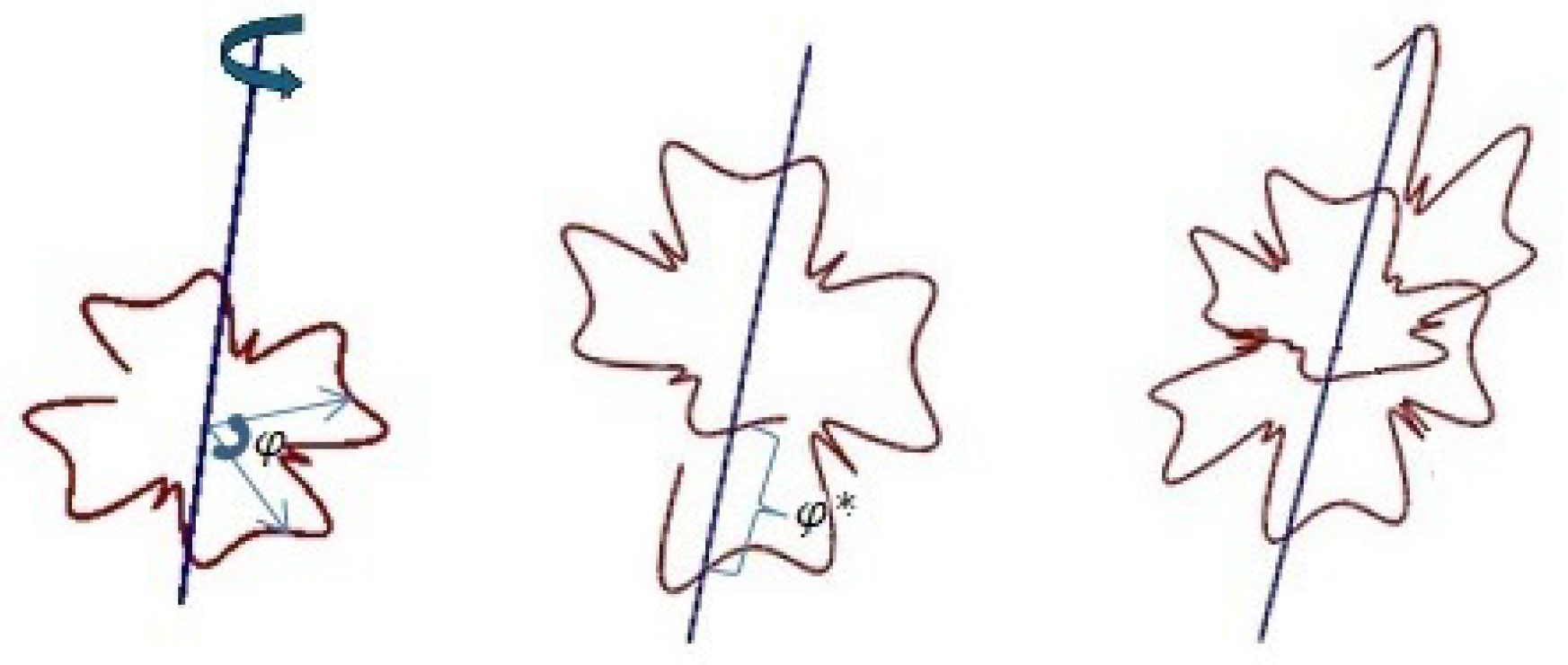
Furthermore, in Figure 2, we give some superelliptic screw motion models for different values of , respectively. □
Figure 2.
Some superelliptic right and left screw motion models for different values of , respectively.
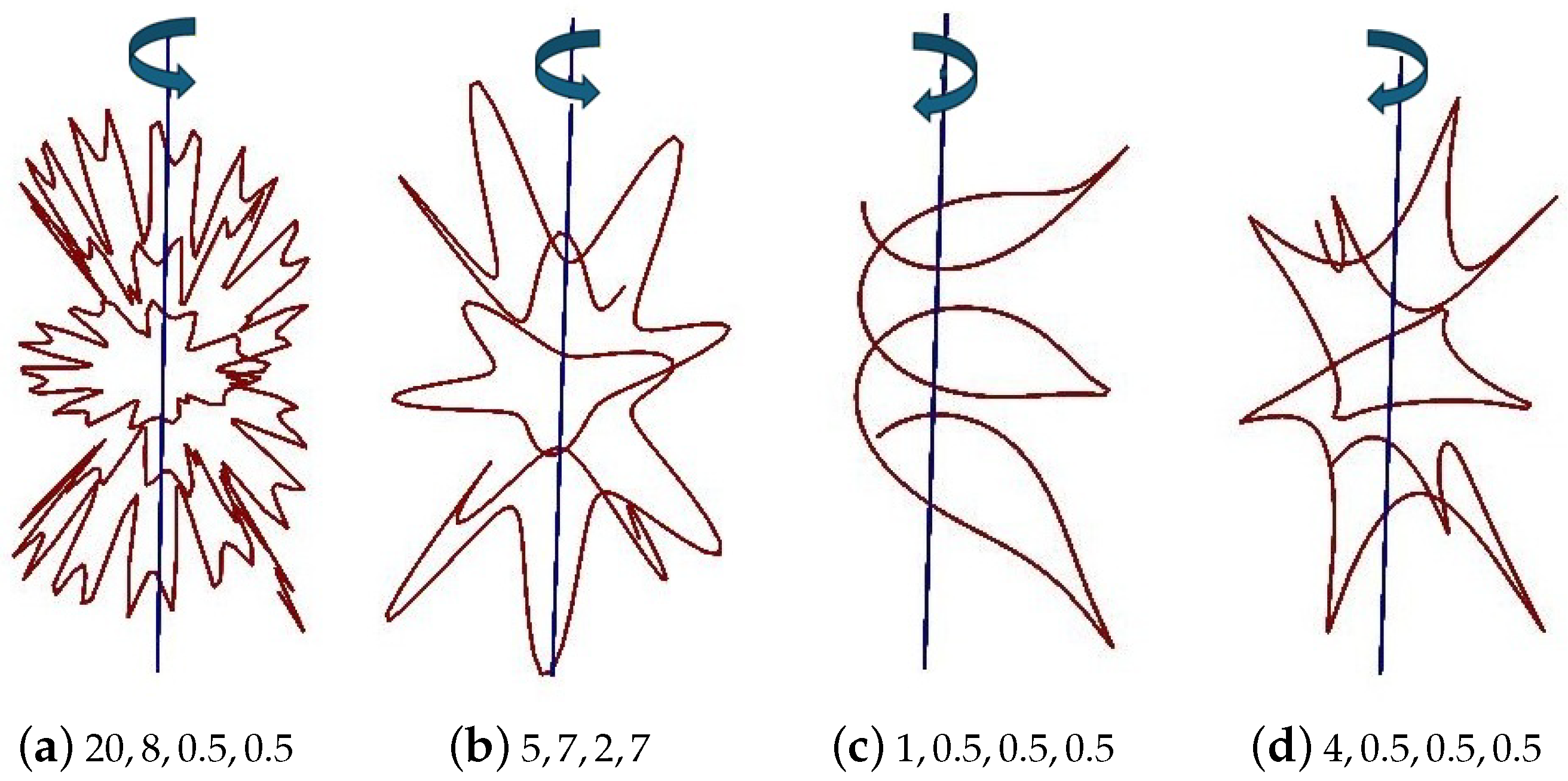
In screw motions defined by standard dual quaternions, when a vector of constant length with respect to the Euclidean metric rotates, the endpoints of this vector trace a circular helix. However, in the superelliptic metric structure considered here, the notion of “constant length” differs fundamentally from the Euclidean norm. Consequently, a vector that has constant length in this space does not preserve a constant Euclidean magnitude; instead, its magnitude is scaled according to the Gielis superformula. Therefore, during a screw motion in the superelliptic space, the endpoints of the rotating superelliptic vector form a circular helix when observed within the intrinsic geometry of the space itself. On the other hand, when the same motion is viewed through the “Euclidean lens,” the resulting trajectories are no longer classical helices but rather more intricate helical curves associated with Gielis-type geometries (seen in Figure 1 and Figure 2). In other words, motions that are geometrically natural and regular in the superelliptic setting appear in Euclidean space as nonlinearly scaled helical trajectories. This perspective demonstrates that screw motions are not restricted solely to classical cylindrical helices; instead, their geometric appearance may vary significantly depending on the underlying metric structure. In particular, superelliptic screw motions provide an important geometric framework for modeling many organic forms, growth patterns, and spiral structures observed in nature. From this viewpoint, the proposed approach offers an effective and extensible method for explaining the formation mechanisms of complex natural shapes. Moreover, in the special case where and for , the proposed superelliptic structure reduces to the classical Euclidean metric framework, and consequently, the standard dual quaternion theory together with its classical kinematic applications is recovered.
5. Conclusions
In this paper, we developed a superelliptic dual quaternion framework by incorporating Gielis’ superformula into the metric and algebraic structure of rigid-body kinematics. Starting from a superelliptic inner product on and its associated vector product, we introduced superelliptic dual numbers and superelliptic dual vectors, thereby extending the classical E-Study correspondence to a superelliptic setting. This construction provides a one-to-one relation between unit superelliptic dual vectors and directed superelliptic lines, and thus establishes the geometric foundation of the proposed theory.
On this basis, we formulated the algebra of superelliptic dual quaternions, including their conjugations, norm, inverse, and polar representation. Within this framework, we derived operators that describe coupled translation and rotation in , showing that rigid motions can be represented consistently with the underlying superelliptic geometry. A further contribution of the study is the introduction of the superelliptic dual angle, which encodes both the angular separation and the shortest distance between directed superelliptic lines in a unified manner.
The main result of the paper is the theorem of superelliptic screw motion. This theorem shows that a unit superelliptic dual quaternion generates a motion consisting of rotation about and translation along a common superelliptic axis, thereby extending the classical Euclidean screw-theoretic interpretation of dual quaternions to a parameter-dependent superelliptic geometry. In this sense, the proposed model does not merely generalize the algebraic formalism, but also enlarges the class of admissible motion profiles and geometric trajectories that can be described within a single compact framework.
The visual realizations obtained for different parameter choices of the Gielis formula further demonstrate the geometric richness and kinematic flexibility of the proposed approach. These examples indicate that the present formulation can capture a wide variety of nonclassical rigid motions associated with superelliptic shapes and axes. Therefore, the theory developed here offers a new mathematical perspective for shape-dependent kinematics and may serve as a useful basis for future studies in robotics, geometric modeling, motion planning, and related applications in which non-Euclidean or nonstandard geometric structures play a central role.
Future studies may extend the proposed framework to higher-dimensional superelliptic or superquadric geometries and develop a corresponding theory of superelliptic rigid-body dynamics. Another important research direction is the systematic investigation of admissible Gielis-parameter domains and singular configurations for stable computation and motion planning. From an applied perspective, the proposed framework may be relevant to applications in robotics, artificial intelligence, computer vision, geometric design, and computational motion modeling. In robotics, many objects and obstacles are more accurately approximated by superelliptic or superquadric shapes than by spheres, cylinders, or classical quadrics. Therefore, a screw-motion formulation adapted to superelliptic geometry may provide useful tools for robotic grasping, obstacle avoidance, robotic manipulation, pose interpolation, and trajectory generation around non-circular profiles. In artificial intelligence and computer vision, the Gielis-parameter-dependent structure may offer compact and flexible shape descriptors for model-based recognition and learning-assisted motion generation. Furthermore, in geometric design and computer-aided modeling, the proposed algebraic operators may be employed to construct controlled shape-dependent trajectories, tool paths, and animation motions associated with superelliptic axes and profiles. Moreover, integrating the present framework with optimization methods, control theory, and learning-based approaches may significantly enhance its practical applicability. Future investigations may also explore approximation-theoretic and wavelet-based operator techniques for the computational realization of superelliptic screw motions and Gielis-type helical trajectories. In this context, operator-based approximation methods may provide efficient numerical frameworks for the representation and approximation of superelliptic geometric motions and related kinematic structures [41,42].
Author Contributions
Conceptualization, E.P. and Z.Ö.; methodology, E.P. and Z.Ö.; software, E.P. and Z.Ö.; validation, E.P. and Z.Ö.; formal analysis, E.P. and Z.Ö.; investigation, E.P. and Z.Ö.; resources, E.P. and Z.Ö.; data curation, E.P. and Z.Ö.; writing—original draft preparation, E.P. and Z.Ö.; writing—review and editing, E.P. and Z.Ö.; visualization, E.P. and Z.Ö.; supervision, Z.Ö.; project administration, Z.Ö. All authors have read and agreed to the published version of the manuscript.
Funding
The authors declare that no funds, grants, or other support was received during the preparation of this manuscript.
Data Availability Statement
No data sets were generated or analyzed during the preparation of the article.
Conflicts of Interest
The authors declare no conflicts of interest.
References
- Lamé, G. Examen des Différentes Méthodes Employées pour Résoudre les Problèmes de Géométrie; Mme. Ve. Courcier, Imprimeur-Libraire: Paris, France, 1818. [Google Scholar]
- Gardiner, M. The superellipse: A curve that lies between the ellipse and the rectangle. Sci. Am. 1965, 213, 222–232. [Google Scholar]
- Flanagan, D.L.; Hefner, O.V. Surface molding—New tool for the engineer (Man-Computer Graphics/MCG/allows operator control through oscilloscope via light sensitive pen). Astronaut. Aeronaut. 1967, 4, 58–62. [Google Scholar]
- Gridgeman, N.T. Lamé ovals. Math. Gaz. 1970, 54, 31–37. [Google Scholar] [CrossRef] [Scilit]
- Matsuura, M. Asymptotic behaviour of the maximum curvature of Lamé curves. J. Geom. Graph. 2014, 18, 45–59. [Google Scholar]
- Barr, A.H. Superquadrics and angle-preserving transformations. IEEE Comput. Graph. Appl. 1981, 1, 11–23. [Google Scholar] [CrossRef] [Scilit]
- Franklin, W.R.; Barr, A.H. Faster calculation of superquadric shapes. IEEE Comput. Graph. Appl. 1981, 1, 41–47. [Google Scholar] [CrossRef] [Scilit]
- Pentland, A.P. Perceptual organization and the representation of natural form. In Readings in Computer Vision; Morgan Kaufmann: Burlington, MA, USA, 1987; Volume 28, pp. 680–699. [Google Scholar]
- Gielis, J. A generic geometric transformation that unifies a wide range of natural and abstract shapes. Am. J. Bot. 2003, 90, 333–338. [Google Scholar] [CrossRef] [Scilit]
- Silva, E.C.E.; Costa, M.F.; Erlhagen, W.; Bicho, E. Superquadrics objects representation for robot manipulation. AIP Conf. Proc. 2016, 1738, 300004. [Google Scholar]
- Tavkhelidze, I.; Cassisa, C.; Gielis, J.; Ricci, P.E. About “bulky” links, generated by generalized Mobius Listing’s bodies [GML. sup. n. sub. 3]. Rend. Lincei-Mat. E Appl. 2013, 24, 11–39. [Google Scholar]
- Gielis, J.; Shi, P.; Beirinckx, B.; Caratelli, D.; Ricci, P.E. Lamé-Gielis curves in biology and geometry. In Proceedings of the 2021 International Conference Riemannian Geometry and Applications (RIGA 2021), Bucharest, Romania, 15–17 January 2021; pp. 5–33. [Google Scholar]
- Gielis, J.; Beirinckx, B.; Bastiaens, E. Superquadrics with rational and irrational symmetry. In Proceedings of the Eighth ACM Symposium on Solid Modeling and Applications; Association for Computing Machinery: New York, NY, USA, 2003; pp. 262–265. [Google Scholar]
- Hamilton, W.R., II. On quaternions; or on a new system of imaginaries in algebra. Dublin Philos. Mag. J. Sci. 1844, 25, 10–13. [Google Scholar]
- Clifford, W.K. Preliminary sketch of biquaternions. Proc. Lond. Math. Soc. 1873, 4, 381–395. [Google Scholar] [CrossRef] [Scilit]
- Cayley, A. On certain results relating to quaternions. Philos. Mag. 1845, 26, 141–145. [Google Scholar]
- Kelland, P.; Tait, P.G. Introduction to Quaternions; Macmillan and Company: London, UK, 1882. [Google Scholar]
- Hardy, A.S. Elements of Quaternions; Ginn, Heath, and Co.: Boston, MA, USA, 1881. [Google Scholar]
- Shoemake, K. Animating rotation with quaternion curves. In Proceedings of the 12th Annual Conference on Computer Graphics and Interactive Techniques; Association for Computing Machinery: New York, NY, USA, 1985; Volume 19, pp. 245–254. [Google Scholar]
- Study, E. Geometrie der Dynamen. Z. Math. Naturwissenschaftlischen Unterr. 1903, 35, 470–483. [Google Scholar]
- McAulay, A. Octonions: A Development of Clifford’s Bi-Quaternions; Cambridge University Press: Cambridge, UK, 1898. [Google Scholar]
- Kuipers, J.B. Quaternions and Rotation Sequences: A Primer with Applications to Orbits, Aerospace, and Virtual Reality; Princeton University Press: Princeton, NJ, USA, 1999. [Google Scholar]
- Vicci, L. Quaternions and Rotations in 3-Space: The Algebra and Geometric Interpretation; Technical Report; UNC: Chapel Hill, NC, USA, 2001. [Google Scholar]
- Ball, R.S. The Theory of Screws: A Study in the Dynamics of a Rigid Body; Hodges, Foster, and Co.: Dublin, Ireland, 1876. [Google Scholar]
- Sariyildiz, E.; Temeltaş, H. A new formulation method for solving kinematic problems of multiarm robot systems using quaternion algebra in the screw theory framework. Turk. J. Electr. Eng. Comput. Sci. 2012, 20, 607–628. [Google Scholar] [CrossRef] [Scilit]
- Leclercq, G.; Lefèvre, P.; Blohm, G. 3D kinematics using dual quaternions: Theory and applications in neuroscience. Front. Behav. Neurosci. 2013, 7, 7. [Google Scholar] [CrossRef] [Scilit] [PubMed]
- Radavelli, L.A.; De Pieri, E.R.; Martins, D.; Simoni, R. Points, lines, screws and planes in dual quaternions kinematics. In Advances in Robot Kinematics; Springer International Publishing: Cham, Switzerland, 2014; pp. 285–293. [Google Scholar]
- Özgür, E.; Mezouar, Y. Kinematic modeling and control of a robot arm using unit dual quaternions. Robot. Auton. Syst. 2016, 77, 66–73. [Google Scholar] [CrossRef] [Scilit]
- Dantam, N.T. Robust and efficient forward, differential, and inverse kinematics using dual quaternions. Int. J. Robot. Res. 2021, 40, 1087–1105. [Google Scholar] [CrossRef] [Scilit]
- Cohen, A.; Shoham, M. Hyper Dual Quaternions representation of rigid bodies kinematics. Mech. Mach. Theory 2020, 150, 103861. [Google Scholar] [CrossRef] [Scilit]
- Abaunza, H.; Chandra, R.; Özgür, E.; Ramon, J.A.C.; Mezouar, Y. Kinematic screws and dual quaternion based motion controllers. Control Eng. Pract. 2022, 128, 105325. [Google Scholar] [CrossRef] [Scilit]
- Kenwright, B. Dual-quaternion interpolation. arXiv 2023, arXiv:2303.13395. [Google Scholar] [CrossRef] [Scilit]
- Teimoorzadeh, A.; Silva, F.F.A.; Figueredo, L.F.; Haddadin, S. Smooth real-time motion planning based on a cascade dual-quaternion screw-geometry MPC. In International Workshop on Human-Friendly Robotics; Springer Nature: Cham, Switzerland, 2023; pp. 164–180. [Google Scholar]
- Farias, J.G.; De Pieri, E.; Martins, D. A review on the applications of dual quaternions. Machines 2024, 12, 402. [Google Scholar] [CrossRef] [Scilit]
- Wang, X.; Sun, H.; Liu, C.; Song, H. Dual quaternion operations for rigid body motion and their application to the hand–eye calibration. Mech. Mach. Theory 2024, 193, 105566. [Google Scholar] [CrossRef] [Scilit]
- Stankovic, A.; Ben-Larbi, M.K.; Müller, W.H. A Dual Quaternion based RRT* Path Planning Approach for Satellite Rendezvous and Docking. IFAC-PapersOnLine 2025, 59, 103–108. [Google Scholar] [CrossRef] [Scilit]
- Weiss, H.; Zivan, Y. Dual-Quaternion Tracking Loops for Spacecraft Screw Motion. J. Guid. Control Dyn. 2026, 49, 852–868. [Google Scholar] [CrossRef] [Scilit]
- Parlak, E.; Özdemir, Z. Superelliptic motion and superelliptic quaternions via Gielis formula. Phys. Scr. 2025, 100, 095212. [Google Scholar] [CrossRef] [Scilit]
- Özdemir, Z.; Parlak, E. Superquadric Motion and Superquadric Hyperbolic Split Quaternion Algebra Via Gielis Formula. Math. Methods Appl. Sci. 2025, 48, 15035–15048. [Google Scholar] [CrossRef] [Scilit]
- Allard, J. Note on squares and cubes. Math. Mag. 1964, 37, 210–214. [Google Scholar] [CrossRef]
- Ayman-Mursaleen, M.; Alshaban, E.; Nasiruzzaman, M. Shape preserving approximation properties to family of α-Bernstein shifted knot operators. J. Inequal. Appl. 2025, 1, 107. [Google Scholar] [CrossRef] [Scilit]
- Ayman-Mursaleen, M. Quadratic function preserving wavelet type Baskakov operators for enhanced function approximation. Comput. Appl. Math. 2025, 44, 395. [Google Scholar] [CrossRef] [Scilit]
Disclaimer/Publisher’s Note: The statements, opinions and data contained in all publications are solely those of the individual author(s) and contributor(s) and not of MDPI and/or the editor(s). MDPI and/or the editor(s) disclaim responsibility for any injury to people or property resulting from any ideas, methods, instructions or products referred to in the content. |
© 2026 by the authors. Licensee MDPI, Basel, Switzerland. This article is an open access article distributed under the terms and conditions of the Creative Commons Attribution (CC BY) license.