Soliton Solutions to a Nonisospectral mKdV-sG Equation with Self-Consistent Sources and Reductions

Abstract

We derive multisoliton solutions for a nonisospectral mKdV-sG equation with self-consistent sources by means of the bilinear approach. This nonisospectral equation is a generic one which is related to a time-dependent spectral parameter with time evolution ${\lambda }_t={\mu }_2\lambda +4{\mu }_3{\lambda }^3+{\nu }_2/\left(4\lambda \right)$. Reductions to some soliton equations with self-consistent sources are investigated. One- and two-soliton solutions for the reduced equations are presented and dynamical behaviors are illustrated.

1. Introduction

Nonisospectral integrable equations play special roles in both mathematics and physics. Unlike isospectral integrable equations, the nonisospectral integrable equations are always associated with time-dependent spectral parameters, namely ${\lambda }_t\ne 0$ [1]. Such equations can be used to model nonlinear wave evolution in nonuniform media [1,2]. In such models, the wave amplitude, velocity, or width may depend on time. Related spectral transform studies also appeared in [3]. In addition, the nonisospectral integrable equations were usually used to generate $\tau$-symmetries [4,5,6,7]. To date, a lot of progress has been achieved on the nonisospectral integrable equations. The inverse scattering transform, Hirota’s method and Darboux transformation were developed systematically to solve the nonisospectral integrable equations [8,9,10,11,12,13,14]. Recently, many classical nonisospectral integrable equations were revisited within the framework of the Cauchy matrix approach [15,16], including the nonisospectral Korteweg–de Vries (KdV) equation, the nonisospectral modified KdV (mKdV) equation, and the nonisospectral sine-Gordon (sG) equation (cf. [17]). Motivated by this work, Tian et al. applied the Cauchy matrix approach to construct three types of nonisospectral matrix mKdV equations and presented their Cauchy matrix structures and solutions. Furthermore, three nonisospectral three-component mKdV equations were obtained, which can be regarded as novel members of the nonisospectral Ablowitz–Kaup–Newell–Segur (AKNS) hierarchy [18]. In [19], Silem et al. interpreted how space-time-localized waves are generated by introducing nonisospectral effects.

Soliton equations with self-consistent sources (SCSs) are of much physical interest. They are employed to depict the propagation of waves with nonconstant velocity and the interaction between different waves. For example, the KdV equation with SCSs describes the interaction of long and short capillary–gravity waves [20] and the Kadomtsev–Petviashvili (KP) equation with SCSs is relevant to some problems in hydrodynamic solid-state physics, plasma physics, etc. [21,22]. In addition, the Yajima–Oikawa system [23] is actually related to $u_t=u_y+$ SCSs in the KP hierarchy with SCSs. Many methods have been developed to obtain the soliton equations with SCSs. One of them is using the high-order constrained flows of soliton equations; in particular, the high-order constrained flows of soliton equations are considered as the stationary equations of the soliton equations with SCSs [24]. With this method, it is easy to obtain the Lax representations of the soliton hierarchies with SCSs. Mathematically, many classical solving methods, such as inverse scattering transform, Darboux transformation, the Hirota method and the Wronskian technique, have been applied to such systems and many explicit exact solutions have been derived [25,26,27,28]. Recently, Tian and Zhang utilized the Cauchy matrix scheme to construct explicit multiple-pole solutions to the multi-component Yajima–Oikawa system, of which there is more freedom in dispersion relations and amplitudes [29]. Subsequently, Li et al. derived the Lakshmanan–Porsezian–Daniel equation with SCSs, whose soliton solutions, breather solutions and rogue wave solutions were obtained via the Darboux transformation [30].

To describe the propagation of few-cycle optical pulses (FCPs) in transparent media, Sazonov [31] introduced the mKdV-sG equation

$$\begin{array}{c}\hfill u_{tx}=-{\mu }_1(u_{xxxx}+{\displaystyle \frac{3}{2}}{u}_x^2{u}_{xx})+{\nu }_{1}sinu\end{array}$$

(1)

by using non-slowly varying envelope approximation, which governs the evolution of an optical FCP in a two-component medium (see also [32]). In (1), both ${\mu }_1$ and ${\nu }_1$ are constants. Leblond and Mihalache showed that all other non-slowly varying envelope approximation models of FCP propagation that can be found in the literature, especially the so-called `short pulse equation’, are in fact approximations or special cases of the mKdV-sG model [33]. In [34], they further gave a review concentrating on theoretical studies performed in the past decade concerning the description of FCP solitons beyond the slowly varying envelope approximation. Like the usual integrable equations, the mKdV-sG Equation (1) also possesses the multisoliton solutions [35,36]. In recent decades, a great deal of attention has been devoted to the study of the mKdV-sG Equation (1), such as nonautonomous soliton solutions [37], breather and soliton molecule solutions [38,39], nonlocal version and linear superposition [40], infinitely many nonlocal symmetries and nonlocal conservation laws [41].

In [42], a general nonisospectral mKdV-sG equation was introduced, which admits several reductions by choosing special parameters. The multisoliton solutions were presented in Hirota’s bilinear method and the Wronskian technique. This combination is useful for two reasons. Physically, the mKdV-sG equation has been used as a model for few-cycle optical pulses beyond the slowly varying envelope approximation. Nonisospectrality is commonly used to describe waves in nonuniform media, where the spectral parameter depends on time. This may affect the soliton’s trajectory, velocity, and, in some reductions, its local width or slope. The SCS terms introduce auxiliary source fields through the eigenfunctions of the associated spectral problem. Thus, the present equation may be viewed as a mathematical model for studying few-cycle pulse dynamics in nonuniform media with self-consistent source effects. Mathematically, it also gives a unified setting to study time-dependent spectral parameters and source effects together. In the present paper, we will generalize those results to the following nonisospectral mKdV-sG equation with SCSs (ni-mKdV-SG-SCSs).

$$\begin{array}{cc}\hfill u_{tx}=& -{\mu }_1(u_{xxxx}+{\displaystyle \frac{3}{2}}{u}_x^2{u}_{xx})+{\mu }_2{(x{u}_x)}_x\hfill \\ \hfill & +{\mu }_3(x(u_{xxxx}+{\displaystyle \frac{3}{2}}{u}_x^2{u}_{xx})+3u_{xxx}+u_x^3+{\displaystyle \frac{1}{2}}{u}_{xx}{\partial }^{-1}{u}_x^2)+{\nu }_{1}sinu\hfill \\ \hfill & +{\nu }_2\left(xsinu-cosu{\partial }^{-1}sinu+sinu{\partial }^{-1}(cosu-1)\right)+2{\displaystyle \sum _{j=1}^N}{({\varphi }_{1j}^2+{\varphi }_{2j}^2)}_x,\hfill \end{array}$$

(2)

$${\varphi }_{1j,x}=-{\lambda }_j{\varphi }_{1j}+{\displaystyle \frac{u_x}{2}}{\varphi }_{2j},{\varphi }_{2j,x}=-{\displaystyle \frac{u_x}{2}}{\varphi }_{1j}+{\lambda }_j{\varphi }_{2j},(j=1,2,\dots ,N),$$

(3)

where ${\partial }^{-1}={\displaystyle \frac{1}{2}}({\int }_{-\infty }^x-{\int }_x^{+\infty })·dx$ denotes the inverse differential operator, ${\lambda }_j={\lambda }_j\left(t\right)$; ${\mu }_1,{\mu }_2,{\mu }_3,{\nu }_1$ and ${\nu }_2$ are parameters, and $\left\{{({\varphi }_{1j}^2+{\varphi }_{2j}^2)}_x\right\}$ are N SCSs. Equation (2) is Lax-integrable and related to a time-dependent spectral parameter $\lambda$ with time evolution ${\lambda }_t={\mu }_2\lambda +4{\mu }_3{\lambda }^3+{\displaystyle \frac{{\nu }_2}{4\lambda }}$ (cf. [42] and see also Section 2). This equation is a general form and contains many special reductions. For example, taking ${\mu }_1={\mu }_2={\mu }_3={\nu }_2=0$ and ${\nu }_1=1$, Equation (2) reduces to

$$u_{tx}=sinu+2{\displaystyle \sum _{j=1}^N}{({\varphi }_{1j}^2+{\varphi }_{2j}^2)}_x.$$

(4)

For this sG-SCSs reduction, the source equations are the same as (3). For this reason, they are not repeated. Here, $\left\{{\lambda }_j\right\}$ are N different eigenvalues. This system is nothing but the sG equation with SCSs (sG-SCSs) and was solved through Hirota’s method and the Wronskian technique [27]. When ${\mu }_2={\mu }_3={\nu }_2=0$, Equation (2) yields the mKdV-sG equation with SCSs (mKdV-sG-SCSs) [43]

$$u_{tx}=-{\mu }_1(u_{xxxx}+{\displaystyle \frac{3}{2}}{u}_x^2{u}_{xx})+{\nu }_{1}sinu+2{\displaystyle \sum _{j=1}^N}{({\varphi }_{1j}^2+{\varphi }_{2j}^2)}_x.$$

(5)

For this mKdV-sG-SCSs reduction, the source equations are also the same as (3), and hence are not repeated. Here, $\left\{{\lambda }_j\right\}$ are N different eigenvalues. When ${\mu }_1={\mu }_2={\nu }_1={\nu }_2=0$ and ${\mu }_3=1$, we obtain the nonisospectral mKdV equation with SCSs (ni-mKdV-SCSs)

$$\begin{array}{cc}\hfill u_{tx}=& x\left(u_{xxxx}+{\displaystyle \frac{3}{2}}{u}_x^2{u}_{xx}\right)+3u_{xxx}+u_x^3+{\displaystyle \frac{1}{2}}{u}_{xx}{\partial }^{-1}{u}_x^2+2{\displaystyle \sum _{j=1}^N}{({\varphi }_{1j}^2+{\varphi }_{2j}^2)}_x.\hfill \end{array}$$

(6)

For this ni-mKdV-SCSs reduction, the source equations are again the same as (3), and therefore are not repeated. This equation is reduced to the one given in [44] via transformation $u_x=v/2$, where $\{{\lambda }_j={\lambda }_j\left(t\right)\}$ are N different eigenvalues.

In this paper, we are interested in multisoliton solutions for the general ni-mKdV-SG-SCS Equation (2). We aim to construct its solutions by means of Hirota’s method. The paper is organized as follows. In Section 2, we describe the Lax integrability of the ni-mKdV-SG-SCS Equation (2). In Section 3, we transform (2) into its bilinear form and solve the bilinear equations by Hirota’s bilinear method. In Section 4, one- and two-soliton solutions for some special reduction equations are presented, and the corresponding dynamical behaviors are illustrated. Section 5 contains the conclusions.

2. Lax Integrability for the ni-mKdV-sG-SCS Equation (2)

Generally speaking, depending on the underlying linear spectral problems, a nonisospectral hierarchy can be derived via the Lax equation, zero-curvature equation, or within the framework of Kac–Moody algebras, among other approaches [45,46,47]. In this section, we show the Lax integrability of the ni-mKdV-sG-SCS Equation (2).

To begin with, we consider the linear spectral problem [48]

$$\begin{array}{c}\hfill {\varphi }_x=M\varphi =\left(\begin{array}{cc}-\lambda & {\displaystyle \frac{u_x}{2}}\\ -{\displaystyle \frac{u_x}{2}}& \lambda \end{array}\right)\varphi ,\end{array}$$

(7)

where $\varphi ={({\varphi }_1,{\varphi }_2)}^{\mathrm{T}}$, $u=u(x,t)$ is the potential function and $\lambda$ is the spectral parameter. For deriving the ni-mKdV-sG-SCS Equation (2), we introduce the time evolution part

$$\begin{array}{c}\hfill {\varphi }_t=N\varphi =\left(\begin{array}{cc}A& B\\ C& -A\end{array}\right)\varphi .\end{array}$$

(8)

The compatibility of (7) and (8), i.e., ${\varphi }_{xt}={\varphi }_{tx}$, yields the zero-curvature equation

$$\begin{array}{c}\hfill M_t-N_x+[M,N]=0,\end{array}$$

(9)

whose components are expressed as

$$\begin{array}{cc}\hfill & A={\displaystyle \frac{1}{2}}{\partial }^{-1}(B+C)u_x+A_0-{\lambda }_{t}x,\hfill \end{array}$$

(10)

$$\begin{array}{cc}\hfill & {\displaystyle \frac{1}{2}}\left(\begin{array}{c}{u}_{xt}\\ -u_{xt}\end{array}\right)=L\left(\begin{array}{c}-B\\ C\end{array}\right)-2\lambda \left(\begin{array}{c}-B\\ C\end{array}\right)-{\lambda }_t\left(\begin{array}{c}x{u}_x\\ x{u}_x\end{array}\right)+A_0\left(\begin{array}{c}{u}_x\\ u_x\end{array}\right),\hfill \end{array}$$

(11)

where

$$\begin{array}{c}\hfill L=\left(\begin{array}{cc}-\partial -{\displaystyle \frac{1}{2}}{u}_x{\partial }^{-1}{u}_x& {\displaystyle \frac{1}{2}}{u}_x{\partial }^{-1}{u}_x\\ -{\displaystyle \frac{1}{2}}{u}_x{\partial }^{-1}{u}_x& \partial +{\displaystyle \frac{1}{2}}{u}_x{\partial }^{-1}{u}_x\end{array}\right),\partial ={\displaystyle \frac{\partial }{\partial x}},\end{array}$$

(12)

is the recursion operator and $A_0=A_0(t,\lambda )$. Assuming

$$\begin{array}{cc}\hfill & \left(\begin{array}{c}-B\\ C\end{array}\right)={\displaystyle \sum _{k=1}^3}\left(\begin{array}{c}-b_{1k}\\ c_{1k}\end{array}\right){\left(2\lambda \right)}^{3-k}+\left(\begin{array}{c}-b_{21}\\ c_{21}\end{array}\right){\left(2\lambda \right)}^{-1}+{\displaystyle \frac{1}{2}}{\displaystyle \sum _{j=1}^N}\left({\displaystyle \frac{p_j}{\lambda +{\lambda }_j}}+{\displaystyle \frac{q_j}{\lambda -{\lambda }_j}}\right),\hfill \end{array}$$

(13)

$$\begin{array}{cc}\hfill & {\lambda }_t={\mu }_2\lambda +4{\mu }_3{\lambda }^3+{\displaystyle \frac{{\nu }_2}{4\lambda }},\hfill \end{array}$$

(14)

$$\begin{array}{cc}\hfill & A_0=4{\mu }_1{\lambda }^3-{\displaystyle \frac{{\nu }_1}{4\lambda }},\hfill \end{array}$$

(15)

with constraints for $\{{\lambda }_j={\lambda }_j\left(t\right)\}$,

$$\begin{array}{c}\hfill \left(\begin{array}{c}{\varphi }_{1j,x}\\ {\varphi }_{2j,x}\end{array}\right)=\left(\begin{array}{cc}-{\lambda }_j& {\displaystyle \frac{u_x}{2}}\\ -{\displaystyle \frac{u_x}{2}}& {\lambda }_j\end{array}\right)\left(\begin{array}{c}{\varphi }_{1j}\\ {\varphi }_{2j}\end{array}\right),(j=1,2,\dots ,N),\end{array}$$

(16)

and taking (13) into (10) and equating the coefficients of ${\left(2\lambda \right)}^k$ and ${\displaystyle \frac{1}{\lambda \pm {\lambda }_j}}$, we obtain

$$\begin{array}{cc}\hfill & \left(\begin{array}{c}-b_{11}\\ c_{11}\end{array}\right)=-{\displaystyle \frac{{\mu }_3}{2}}\left(\begin{array}{c}x{u}_x\\ x{u}_x\end{array}\right)+{\displaystyle \frac{{\mu }_1}{2}}\left(\begin{array}{c}{u}_x\\ u_x\end{array}\right),\hfill \end{array}$$

(17)

$$\begin{array}{cc}\hfill & \left(\begin{array}{c}-b_{12}\\ c_{12}\end{array}\right)=-{\displaystyle \frac{{\mu }_3}{2}}L\left(\begin{array}{c}x{u}_x\\ x{u}_x\end{array}\right)+{\displaystyle \frac{{\mu }_1}{2}}L\left(\begin{array}{c}{u}_x\\ u_x\end{array}\right),\hfill \end{array}$$

(18)

$$\begin{array}{cc}\hfill & \left(\begin{array}{c}-b_{13}\\ c_{13}\end{array}\right)=-{\displaystyle \frac{{\mu }_3}{2}}{L}^2\left(\begin{array}{c}x{u}_x\\ x{u}_x\end{array}\right)+{\displaystyle \frac{{\mu }_1}{2}}{L}^2\left(\begin{array}{c}{u}_x\\ u_x\end{array}\right)-{\displaystyle \frac{{\mu }_2}{2}}\left(\begin{array}{c}x{u}_x\\ x{u}_x\end{array}\right),\hfill \end{array}$$

(19)

$$\begin{array}{cc}\hfill & \left(\begin{array}{c}-b_{21}\\ c_{21}\end{array}\right)={\displaystyle \frac{{\nu }_1}{2}}{L}^{-1}\left(\begin{array}{c}{u}_x\\ u_x\end{array}\right)+{\displaystyle \frac{{\nu }_2}{2}}{L}^{-1}\left(\begin{array}{c}x{u}_x\\ x{u}_x\end{array}\right),\hfill \end{array}$$

(20)

$$\begin{array}{cc}\hfill \left(\begin{array}{c}{u}_{xt}\\ -u_{xt}\end{array}\right)=& {\mu }_1{L}^3\left(\begin{array}{c}{u}_x\\ u_x\end{array}\right)-{\mu }_{2}L\left(\begin{array}{c}x{u}_x\\ x{u}_x\end{array}\right)-{\mu }_3{L}^3\left(\begin{array}{c}x{u}_x\\ x{u}_x\end{array}\right)-{\nu }_1{L}^{-1}\left(\begin{array}{c}{u}_x\\ u_x\end{array}\right)\hfill \\ & -{\nu }_2{L}^{-1}\left(\begin{array}{c}x{u}_x\\ x{u}_x\end{array}\right)-2{\displaystyle \sum _{j=1}^N}(p_j+q_j),\hfill \end{array}$$

(21)

$$\begin{array}{cc}\hfill & L{p}_j=-2{\lambda }_j{p}_j,L{q}_j=2{\lambda }_j{q}_j,(j=1,2,\dots ,N).\hfill \end{array}$$

(22)

We take

$$\begin{array}{c}\hfill p_j=-2{\lambda }_j{({\varphi }_{2j}^2,{\varphi }_{1j}^2)}^T,q_j=2{\lambda }_j{({\varphi }_{1j}^2,{\varphi }_{2j}^2)}^T,\end{array}$$

(23)

and write down the ni-mKdV-sG-SCS Equation (2)

$$\begin{array}{cc}\hfill u_{xt}& =-{\mu }_{1}F{u}_{xx}+{\mu }_2{\left(x{u}_x\right)}_x+{\mu }_{3}F{\left(x{u}_x\right)}_x+{\nu }_1{F}^{-1}{u}_{xx}+{\nu }_2{F}^{-1}{\left(x{u}_x\right)}_x\hfill \\ & +2{\displaystyle \sum _{j=1}^N}{({\varphi }_{1j}^2+{\varphi }_{2j}^2)}_x,\hfill \end{array}$$

(24)

$$\begin{array}{cc}\hfill & {\varphi }_{1j,x}=-{\lambda }_j{\varphi }_{1j}+{\displaystyle \frac{u_x}{2}}{\varphi }_{2j},{\varphi }_{2j,x}=-{\displaystyle \frac{u_x}{2}}{\varphi }_{1j}+{\lambda }_j{\varphi }_{2j},(j=1,2,\dots ,N),\hfill \end{array}$$

(25)

where operator F and the inverse $F^{-1}$ are of the form

$$\begin{array}{c}\hfill F={\partial }^2+\partial u_x{\partial }^{-1}{u}_x,F^{-1}=cosu{\partial }^{-1}cosu{\partial }^{-1}+sinu{\partial }^{-1}sinu{\partial }^{-1}.\end{array}$$

(26)

Then, we trace back to obtain

$$\begin{array}{cc}\hfill & A={\displaystyle \frac{1}{2}}\left({\mu }_1{u}_x^2-2{\mu }_{2}x-{\mu }_3(x{u}_x^2+{\partial }^{-1}{u}_x^2)\right)\lambda +{\displaystyle \frac{1}{4\lambda }}\left(-{\nu }_{1}cosu-{\nu }_{2}xcosu-{\nu }_2{\partial }^{-1}usinu\right)\hfill \\ \hfill & +4({\mu }_1-{\mu }_{3}x){\lambda }^3+{\displaystyle \sum _{j=1}^N}{\displaystyle \frac{\lambda {\lambda }_j}{{\lambda }^2-{\lambda }_j^2}}{\partial }^{-1}({\varphi }_{2j}^2-{\varphi }_{1j}^2)u_x,\hfill \end{array}$$

(27)

$$\begin{array}{cc}\hfill & B=-{\displaystyle \frac{{\mu }_1}{4}}(2u_{xxx}+u_x^3)+{\displaystyle \frac{{\mu }_3}{4}}(4u_{xx}+2x{u}_{xxx}+x{u}_x^3+u_x{\partial }^{-1}{u}_x^2)\hfill \\ \hfill & +{\displaystyle \frac{{\mu }_2}{2}}x{u}_x+({\mu }_1{u}_{xx}-{\mu }_3{\left(x{u}_x\right)}_x)\lambda -2({\mu }_1{u}_x-{\mu }_{3}x{u}_x){\lambda }^2\hfill \\ \hfill & +{\displaystyle \frac{{\nu }_1}{4\lambda }}sinu+{\displaystyle \frac{{\nu }_2}{4\lambda }}\left(xsinu-cosu{\partial }^{-1}sinu+sinu{\partial }^{-1}(cosu-1)\right)\hfill \\ \hfill & +{\displaystyle \sum _{j=1}^N}\left({\displaystyle \frac{{\lambda }_j}{\lambda +{\lambda }_j}}{\varphi }_{2j}^2-{\displaystyle \frac{{\lambda }_j}{\lambda -{\lambda }_j}}{\varphi }_{1j}^2\right),\hfill \end{array}$$

(28)

$$\begin{array}{cc}\hfill & C={\displaystyle \frac{{\mu }_1}{4}}(2u_{xxx}+u_x^3)-{\displaystyle \frac{{\mu }_3}{4}}(4u_{xx}+2x{u}_{xxx}+x{u}_x^3+u_x{\partial }^{-1}{u}_x^2)\hfill \\ \hfill & -{\displaystyle \frac{{\mu }_2}{2}}x{u}_x+({\mu }_1{u}_{xx}-{\mu }_3{\left(x{u}_x\right)}_x)\lambda +2({\mu }_1{u}_x-{\mu }_{3}x{u}_x){\lambda }^2\hfill \\ \hfill & +{\displaystyle \frac{{\nu }_1}{4\lambda }}sinu+{\displaystyle \frac{{\nu }_2}{4\lambda }}\left(xsinu-cosu{\partial }^{-1}sinu+sinu{\partial }^{-1}(cosu-1)\right)\hfill \\ \hfill & +{\displaystyle \sum _{j=1}^N}\left(-{\displaystyle \frac{{\lambda }_j}{\lambda +{\lambda }_j}}{\varphi }_{1j}^2+{\displaystyle \frac{{\lambda }_j}{\lambda -{\lambda }_j}}{\varphi }_{2j}^2\right).\hfill \end{array}$$

(29)

Equations (7) and (8) together with (27) provide the Lax pair of Equation (2).

3. Bilinear Form and Solution in Hirota’s Form

In this section, we transform the ni-mKdV-sG-SCS Equation (2) into its bilinear form and construct the multisoliton solutions in Hirota’s form.

3.1. Bilinear Form

Through the transformation of dependent variables,

$$\begin{array}{c}\hfill u=2iln{\displaystyle \frac{f^{*}}{f}},{\varphi }_{1j}={\displaystyle \frac{g_j^{*}}{f^{*}}}+{\displaystyle \frac{g_j}{f}},{\varphi }_{2j}=i\left({\displaystyle \frac{g_j^{*}}{f^{*}}}-{\displaystyle \frac{g_j}{f}}\right),(j=1,2,\dots ,N),\end{array}$$

(30)

where $f^{*}$ and $g_j^{*}$ are the complex conjugates of f and $g_j$, respectively, and i is the imaginary unit, Equation (2) is bilinearized as

$$\begin{array}{cc}\hfill 2D_t{D}_{x}f·f=& -2{\mu }_1{D}_x^{4}f·f+2x{\mu }_2{D}_x^{2}f·f+4{\mu }_{2}f{f}_x+({\nu }_1+x{\nu }_2)(f^2-f^{{*}^2})\hfill \\ \hfill & +2{\mu }_3(x{D}_x^{4}f·f+fh+4D_x{f}_{xx}·f)-{\nu }_2{f}^{*}g-16i{\displaystyle \sum _{j=1}^N}{\lambda }_j{g}_j^2,\hfill \end{array}$$

(31)

$$\begin{array}{cc}\hfill D_{x}h·f=& D_x^{4}f·f,\hfill \end{array}$$

(32)

$$\begin{array}{cc}\hfill D_{x}g·f^{*}=& f^2-f^{{*}^2},\hfill \end{array}$$

(33)

$$\begin{array}{cc}\hfill D_x^{2}f·f^{*}=& 0,\hfill \end{array}$$

(34)

$$\begin{array}{cc}\hfill D_x{g}_j^{*}·f=& -{\lambda }_j{g}_j{f}^{*},(j=1,2,\dots ,N),\hfill \end{array}$$

(35)

where g and h are auxiliary functions and D is the well-known Hirota’s bilinear operator defined by [49]

$$\begin{array}{c}\hfill D_t^m{D}_x^{n}a·b={({\partial }_t-{\partial }_{t^{\prime }})}^m{({\partial }_x-{\partial }_{x^{\prime }})}^{n}a(t,x)b(t^{\prime },x^{\prime }){|}_{t^{\prime }=t,x^{\prime }=x}.\end{array}$$

(36)

We expand $f,g,h$ and $g_j$ as

$$\begin{array}{c}\hfill f=1+{\displaystyle \sum _{k=1}^{\infty }}{f}^{\left(2k\right)}{\epsilon }^{2k},g={\displaystyle \sum _{k=1}^{\infty }}{g}^{\left(2k\right)}{\epsilon }^{2k},h={\displaystyle \sum _{k=1}^{\infty }}{h}^{\left(2k\right)}{\epsilon }^{2k},g_j={\displaystyle \sum _{k=1}^{\infty }}{g}_j^{(2k-1)}{\epsilon }^{2k-1}\end{array}$$

(37)

and take

$$\begin{array}{c}\hfill g_j^{\left(1\right)}=\sqrt{{\beta }_j\left(t\right)}{e}^{{\xi }_j},{\xi }_j=k_j\left(t\right)x+w_j\left(t\right)+{\int }_0^t{\beta }_j\left(z\right)dz+{\xi }_j^{\left(0\right)},(j=1,2,\dots ,N).\end{array}$$

(38)

Substituting the expansion (37) into (31) and equating the coefficients of each ${\epsilon }^k$, we have

$$\begin{array}{cc}\hfill & 2f_{xt}^{\left(2\right)}=-2{\mu }_1{f}_{xxxx}^{\left(2\right)}+2x{\mu }_2{f}_{xx}^{\left(2\right)}+2{\mu }_2{f}_x^{\left(2\right)}+{\mu }_3(2x{f}_{xxxx}^{\left(2\right)}+4f_{xxx}^{\left(2\right)}+h^{\left(2\right)})\hfill \\ \hfill & +{\nu }_1(f^{\left(2\right)}-f^{{\left(2\right)}^{*}})+x{\nu }_2(f^{\left(2\right)}-f^{{\left(2\right)}^{*}})-{\displaystyle \frac{{\nu }_2}{2}}{g}^{\left(2\right)}-8i{\displaystyle \sum _{j=1}^N}{\lambda }_j{g}_j^{{\left(1\right)}^2},\hfill \end{array}$$

(39)

$$\begin{array}{cc}\hfill & 2f_{xxxx}^{\left(2\right)}=h_x^{\left(2\right)},\hfill \end{array}$$

(40)

$$\begin{array}{cc}\hfill & g_x^{\left(2\right)}=2(f^{\left(2\right)}-f^{{\left(2\right)}^{*}}),\hfill \end{array}$$

(41)

$$\begin{array}{cc}\hfill & f_{xx}^{\left(2\right)}+f_{xx}^{{\left(2\right)}^{*}}=0,\hfill \end{array}$$

(42)

$$\begin{array}{cc}\hfill & g_{j,x}^{{\left(1\right)}^{*}}=-{\lambda }_j{g}_j^{\left(1\right)},\hfill \end{array}$$

(43)

The coefficients at higher orders of $\epsilon$ can be obtained by an analogous calculation, and are not listed here.

3.2. Multisoliton Solution

Assume that $g_j^{\left(1\right)}$ has the form

$$\begin{array}{c}\hfill g_j^{\left(1\right)}=\sqrt{{\beta }_j\left(t\right)}{e}^{{\xi }_j},{\xi }_j=k_j\left(t\right)x+w_j\left(t\right)+{\int }_0^t{\beta }_j\left(z\right)dz+{\xi }_j^{\left(0\right)},(j=1,2,\dots ,N),\end{array}$$

(44)

where $\left\{k_j\left(t\right)\right\}$ and $\left\{{\omega }_j\left(t\right)\right\}$ are undetermined functions, $\left\{{\beta }_j\left(t\right)\right\}$ are arbitrary continuous real functions of t and $\left\{{\xi }_j^{\left(0\right)}\right\}$ are real constants. If ${\beta }_j\left(t\right)\ge 0$, the source fields ${\varphi }_{1j}$ and ${\varphi }_{2j}$ are real-valued. If ${\beta }_j\left(t\right)<0$ on some interval, the factor $\sqrt{{\beta }_j\left(t\right)}$ becomes purely imaginary. Then, the source fields become complex-valued, while u remains real. In this paper, we treat such source fields as a mathematical extension of the integrable source system. We do not assign a direct physical meaning to these complex-valued source fields here. This convention is used only when the chosen source functions ${\beta }_j\left(t\right)$ take negative values in the examples below.

When $N=1$ in (38), i.e.,

$$\begin{array}{c}\hfill g_1^{\left(1\right)}=\sqrt{{\beta }_1\left(t\right)}{e}^{{\xi }_1},{\xi }_1=k_1\left(t\right)x+w_1\left(t\right)+{\int }_0^t{\beta }_1\left(z\right)dz+{\xi }_1^{\left(0\right)},\end{array}$$

(45)

from (39), we obtain

$$\begin{array}{c}\hfill {\lambda }_1=-k_1\left(t\right),f^{\left(2\right)}=e^{2{\xi }_1+{\displaystyle \frac{\pi }{2}}i},h^{\left(2\right)}=16i{k}_1^3\left(t\right)e^{2{\xi }_1},g^{\left(2\right)}={\displaystyle \frac{2i}{k_1\left(t\right)}}{e}^{2{\xi }_1},\end{array}$$

(46)

where $k_1\left(t\right)$ and ${\omega }_1\left(t\right)$ follow the time evolutions

$$\begin{array}{cc}\hfill & k_{j,t}\left(t\right)={\mu }_2{k}_j\left(t\right)+{\displaystyle \frac{{\nu }_2}{4k_j\left(t\right)}}+4{\mu }_3{k}_j^3\left(t\right),\hfill \end{array}$$

(47)

$$\begin{array}{cc}\hfill & {\omega }_{j,t}\left(t\right)=-4{\mu }_1{k}_j^3\left(t\right)+{\displaystyle \frac{{\nu }_1}{4k_j\left(t\right)}}-{\displaystyle \frac{{\nu }_2}{4k_j^2\left(t\right)}}+4{\mu }_3{k}_j^2\left(t\right).\hfill \end{array}$$

(48)

Furthermore, we know $f^{\left(2k\right)}=g^{\left(2k\right)}=h^{\left(2k\right)}=g_1^{(2k-1)}=0,(k\ge 2)$. Thus, from (30), we obtain the one-soliton solution

$$\begin{array}{c}\hfill u=2iln{\displaystyle \frac{1-i{e}^{2{\xi }_1}}{1+i{e}^{2{\xi }_1}}}=4arctan{e}^{2{\xi }_1},\end{array}$$

(49)

with sources

$$\begin{array}{c}\hfill {\varphi }_{11}=\sqrt{{\beta }_1\left(t\right)}{e}^{-{\xi }_1}sech2{\xi }_1,{\varphi }_{21}=-\sqrt{{\beta }_1\left(t\right)}{e}^{{\xi }_1}sech2{\xi }_1,\end{array}$$

(50)

where we have taken $\epsilon =1$.

When $N=2$, (38) becomes

$$\begin{array}{c}\hfill g_j^{\left(1\right)}=\sqrt{{\beta }_j\left(t\right)}{e}^{{\xi }_j},{\xi }_j=k_j\left(t\right)x+w_j\left(t\right)+{\int }_0^t{\beta }_j\left(z\right)dz+{\xi }_j^{\left(0\right)},(j=1,2),\end{array}$$

(51)

from (39), we have

$$\begin{array}{cc}\hfill & {\lambda }_j=-k_j\left(t\right),(j=1,2),f^{\left(2\right)}=e^{2{\xi }_1+{\displaystyle \frac{\pi }{2}}i}+e^{2{\xi }_2+{\displaystyle \frac{\pi }{2}}i},\hfill \end{array}$$

(52)

$$\begin{array}{cc}\hfill & h^{\left(2\right)}=16i{k}_1^3\left(t\right)e^{2{\xi }_1}+16i{k}_2^3\left(t\right)e^{2{\xi }_2},g^{\left(2\right)}={\displaystyle \frac{2i}{k_1\left(t\right)}}{e}^{2{\xi }_1}+{\displaystyle \frac{2i}{k_2\left(t\right)}}{e}^{2{\xi }_2},\hfill \end{array}$$

(53)

and

$$\begin{array}{cc}\hfill & f^{\left(4\right)}=e^{2{\xi }_1+2{\xi }_2+i\pi +A_{12}},g^{\left(4\right)}=2{\displaystyle \frac{k_1\left(t\right)+k_2\left(t\right)}{k_1\left(t\right)k_2\left(t\right)}}{e}^{2{\xi }_1+2{\xi }_2+A_{12}},\hfill \end{array}$$

(54)

$$\begin{array}{cc}\hfill & h^{\left(4\right)}=-16(k_1\left(t\right)+k_2\left(t\right))(k_1^2\left(t\right)+k_2^2\left(t\right)-k_1\left(t\right)k_2\left(t\right))e^{2{\xi }_1+2{\xi }_2+A_{12}},\hfill \end{array}$$

(55)

$$\begin{array}{cc}\hfill & g_1^{\left(3\right)}=i\sqrt{{\beta }_1\left(t\right)}{\displaystyle \frac{k_1\left(t\right)-k_2\left(t\right)}{k_1\left(t\right)+k_2\left(t\right)}}{e}^{{\xi }_1+2{\xi }_2},g_2^{\left(3\right)}=-i\sqrt{{\beta }_2\left(t\right)}{\displaystyle \frac{k_1\left(t\right)-k_2\left(t\right)}{k_1\left(t\right)+k_2\left(t\right)}}{e}^{2{\xi }_1+{\xi }_2},\hfill \end{array}$$

(56)

and finally catch $f^{\left(2k\right)}=g^{\left(2k\right)}=h^{\left(2k\right)}=g_1^{(2k-1)}=g_2^{(2k-1)}=0,(k\ge 3)$, where $k_j\left(t\right)$ and $w_j\left(t\right)$ are still defined as (47) and

$$\begin{array}{c}\hfill e^{A_{12}}={\left({\displaystyle \frac{k_1\left(t\right)-k_2\left(t\right)}{k_1\left(t\right)+k_2\left(t\right)}}\right)}^2.\end{array}$$

(57)

In this case, the truncated series

$$\begin{array}{c}\hfill f=1+f^{\left(2\right)}+f^{\left(4\right)},g=g^{\left(2\right)}+g^{\left(4\right)},h=h^{\left(2\right)}+h^{\left(4\right)},g_j=g_j^{\left(1\right)}+g_j^{\left(3\right)},(j=1,2)\end{array}$$

(58)

provide a two-soliton solution for (2) through transformation (30).

A general form of the N-soliton solution is expressed as

$$\begin{array}{cc}\hfill f=& \sum _{\rho =0,1}exp\left({\displaystyle \sum _{s=1}^N}{\rho }_s\left(2{\xi }_s+{\displaystyle \frac{\pi }{2}}i\right)+{\displaystyle \sum _{1\le s<l}^N}{\rho }_s{\rho }_l{A}_{sl}\right),\hfill \end{array}$$

(59)

$$\begin{array}{cc}\hfill g_j=& \sqrt{{\beta }_j\left(t\right)}{e}^{{\xi }_j}\sum _{\rho =0,1}{\rho }_{j}exp({\displaystyle \sum _{s=1}^{j-1}}{\rho }_s\left(2{\xi }_s+{\displaystyle \frac{1}{2}}{A}_{sl}+{\displaystyle \frac{\pi }{2}}i\right)+{\displaystyle \sum _{s=j+1}^N}{\rho }_s\left(2{\xi }_s+{\displaystyle \frac{1}{2}}{A}_{sl}-{\displaystyle \frac{\pi }{2}}i\right)\hfill \\ \hfill & +{\displaystyle \sum _{1\le s<l,s,l\ne j}^N}{\rho }_s{\rho }_l{A}_{sl}),(j=1,2,\dots ,N),\hfill \end{array}$$

(60)

where expressions for g and h are omitted; $k_j\left(t\right)$ and $w_j\left(t\right)$ are determined by (47) and

$$\begin{array}{c}\hfill {\lambda }_j=-k_j\left(t\right),e^{A_{jl}}={\left({\displaystyle \frac{k_j\left(t\right)-k_l\left(t\right)}{k_j\left(t\right)+k_l\left(t\right)}}\right)}^2,(1\le j<l\le N),\end{array}$$

(61)

and the sum over $\rho =0,1$ is taken over all possible combinations of ${\rho }_j=0,1,(j=1,2,\dots ,N)$.

The explicit forms of $k_j\left(t\right)$ and $w_j\left(t\right)$ satisfying (47) can be given as

$$\begin{array}{cc}\hfill k_j\left(t\right)=& {\displaystyle \frac{1}{2\sqrt{2{\mu }_3}}}{\left(\kappa tan(\kappa t+\kappa c_j)-{\mu }_2\right)}^{{\displaystyle \frac{1}{2}}},\hfill \end{array}$$

(62)

$$\begin{array}{cc}\hfill w_j\left(t\right)=& \left({\displaystyle \frac{{\mu }_{1}i}{4{\mu }_3\sqrt{2{\mu }_3}\kappa }}{({\mu }_2-i\kappa )}^{{\displaystyle \frac{3}{2}}}-{\displaystyle \frac{\sqrt{2{\mu }_3}{\nu }_{1}i}{2\kappa \sqrt{{\mu }_2-i\kappa }}}\right){\varrho }^{+}\left(t\right)\hfill \\ \hfill & +\left({\displaystyle \frac{-{\mu }_{1}i}{4{\mu }_3\sqrt{2{\mu }_3}\kappa }}{({\mu }_2+i\kappa )}^{{\displaystyle \frac{3}{2}}}+{\displaystyle \frac{\sqrt{2{\mu }_3}{\nu }_{1}i}{2\kappa \sqrt{{\mu }_2+\kappa i}}}\right){\varrho }^{-}\left(t\right)\hfill \\ \hfill & -{\displaystyle \frac{{\mu }_1}{2{\mu }_3\sqrt{2{\mu }_3}}}{\left(\kappa tan(\kappa t+\kappa c_j)-{\mu }_2\right)}^{{\displaystyle \frac{1}{2}}}\hfill \\ \hfill & -{\displaystyle \frac{{\mu }_3{\nu }_2}{\kappa ({\kappa }^2+{\mu }_2^2)}}(-2{\mu }_2(\kappa t+\kappa c_j)+2\kappa lncos(\kappa t+\kappa c_j)\hfill \\ \hfill & +2\kappa ln({\mu }_2-\kappa tan(\kappa t+\kappa c_j)))-{\displaystyle \frac{{\mu }_2}{2}}t-{\displaystyle \frac{1}{2}}lncos(\kappa t+\kappa c_j),\hfill \end{array}$$

(63)

where

$$\begin{array}{c}\hfill \kappa =\sqrt{4{\mu }_3{\nu }_2-{\mu }_2^2},{\varrho }^{\pm }\left(t\right)=arctan{\displaystyle \frac{\sqrt{-{\mu }_2+\kappa tan(\kappa t+\kappa c_j)}}{\sqrt{{\mu }_2\mp \kappa i}}},\end{array}$$

(64)

and $\left\{c_j\right\}$ are constants. For numerical evaluation, the branches of the square-root and arctangent functions in ${\varrho }^{\pm }\left(t\right)$ should be chosen consistently on the time interval under consideration. With this choice, $k_j\left(t\right)$ and $w_j\left(t\right)$ stay continuous as long as the interval does not cross branch cuts or singular points. In particular, the interval should avoid the singular points of the tangent and logarithmic factors.

4. Some Reductions

In this section, we pay attention to one- and two-soliton solutions for several reduced equations. These solutions are obtained from (59) by taking $N=1,2$ and by selecting the parameters ${\mu }_1$, ${\mu }_2$, ${\mu }_3$, ${\nu }_1$ and ${\nu }_2$ in (47). We use the following reduction rule. First, the parameters in the original equation are fixed. The reduced form of (47) then gives the evolution equations for $k_j\left(t\right)$ and $w_j\left(t\right)$. Their explicit expressions are obtained from these equations in each case. Thus, $k_j\left(t\right)$ and $w_j\left(t\right)$ are not chosen independently. Next, the tau function f and the functions g, h, $g_j$ and $h_j$ are obtained by substituting the reduced functions $k_j\left(t\right)$ and $w_j\left(t\right)$ into the general Hirota N-soliton formula. No extra ansatz is imposed on f in the reductions. We only require that the resulting tau functions are explicit and are evaluated on parameter and time intervals where the solution is well-defined. In the examples below, the functions ${\beta }_j\left(t\right)$ are chosen as real continuous source functions. This choice makes the phase integrals well-defined and keeps the source fields explicit. Different choices of ${\beta }_j\left(t\right)$ are then used to show stationary, moving, accelerating and degenerate soliton behaviors. We focus in particular on the dynamical behaviors of the resulting one- and two-soliton solutions.

For each elementary soliton phase ${\xi }_j=k_j\left(t\right)x+w_j\left(t\right)+{\int }_0^t{\beta }_j\left(z\right)dz+{\xi }_j^{\left(0\right)}$, the center can be described by the level curve ${\xi }_j=0$. Hence,

$$\begin{array}{c}\hfill x_j\left(t\right)=-{\displaystyle \frac{w_j\left(t\right)+{\int }_0^t{\beta }_j\left(z\right)dz+{\xi }_j^{\left(0\right)}}{k_j\left(t\right)}}.\end{array}$$

(65)

The corresponding instantaneous velocity is

$$\begin{array}{c}\hfill x_j^{\prime }\left(t\right)=-{\displaystyle \frac{(w_j^{\prime }\left(t\right)+{\beta }_j\left(t\right))k_j\left(t\right)-k_j^{\prime }\left(t\right)\left(w_j\left(t\right)+{\int }_0^t{\beta }_j\left(z\right)dz+{\xi }_j^{\left(0\right)}\right)}{k_j^2\left(t\right)}}.\end{array}$$

(66)

These formulas help us track the background trajectory and velocity of each elementary soliton component. In the isospectral reductions, $k_j\left(t\right)$ is constant. Thus, ${\beta }_j\left(t\right)$ changes the velocity mainly through the phase integral ${\int }_0^t{\beta }_j\left(z\right)dz$. In the nonisospectral reductions, the term containing $k_j^{\prime }\left(t\right)$ gives an additional time-dependent effect. It may lead to acceleration, trajectory bending and changes in the local width or slope. Hence, the two-soliton interaction is not only a usual phase-shift process. It also reflects the time dependence of $k_j\left(t\right)$ and $w_j\left(t\right)$ in the nonisospectral system.

(I). If ${\mu }_1={\mu }_2={\mu }_3={\nu }_2=0,{\nu }_1=1$, we arrive at the sG-SCS Equation (4). In this case, $k_j\left(t\right)=c_j$ and ${\omega }_j\left(t\right)={\displaystyle \frac{t}{4c_j}}$ lead to

$$\begin{array}{c}\hfill {\xi }_j=c_{j}x+{\displaystyle \frac{t}{4c_j}}+{\int }_0^t{\beta }_j\left(z\right)dz+{\xi }_j^{\left(0\right)}.\end{array}$$

(67)

The one-soliton solution reads

$$\begin{array}{c}\hfill u=4arctan{e}^{2{\xi }_1},\end{array}$$

(68)

with the corresponding sources

$$\begin{array}{c}\hfill {\varphi }_{11}=\sqrt{{\beta }_1\left(t\right)}{e}^{-{\xi }_1}sech2{\xi }_1,{\varphi }_{21}=-\sqrt{{\beta }_1\left(t\right)}{e}^{{\xi }_1}sech2{\xi }_1.\end{array}$$

(69)

Solution (68) is a kink soliton with wave span $2\pi$. The inflexion point is located at

$$\begin{array}{c}\hfill \left(x=-{\displaystyle \frac{1}{4c_1^2}}t-{\displaystyle \frac{1}{c_1}}{\int }_0^t{\beta }_1\left(z\right)dz-{\displaystyle \frac{{\xi }_1^{\left(0\right)}}{c_1}},t\right),\end{array}$$

(70)

at which $u\equiv \pi$. The time-dependent wave speed is

$$\begin{array}{c}\hfill {\displaystyle \frac{dx\left(t\right)}{dt}}=-{\displaystyle \frac{1}{4c_1^2}}-{\displaystyle \frac{{\beta }_1\left(t\right)}{c_1}},\end{array}$$

(71)

and the slope of the wave at the inflexion point is

$$\begin{array}{c}\hfill {\displaystyle \frac{du(x,t)}{dx}}=4c_1.\end{array}$$

(72)

The real-valued function ${\beta }_1\left(t\right)$ acts as a source term, which alters the propagation velocity of the soliton and modulates the amplitudes of the source fields through $\sqrt{{\beta }_1\left(t\right)}$.

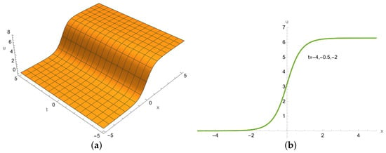
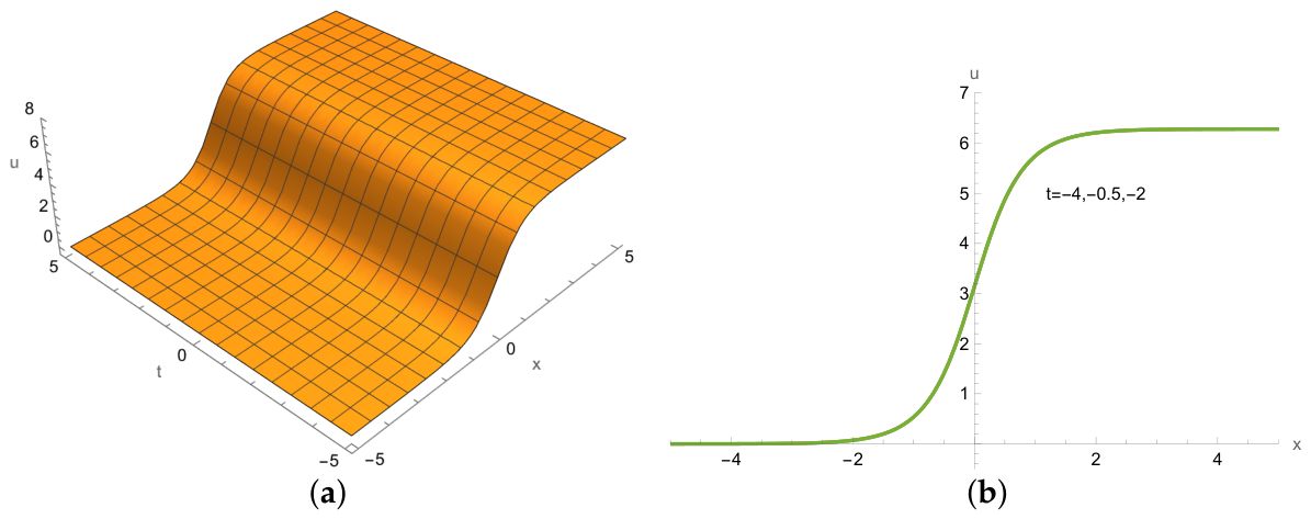
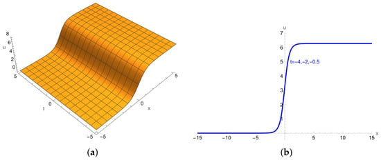
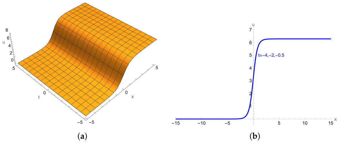
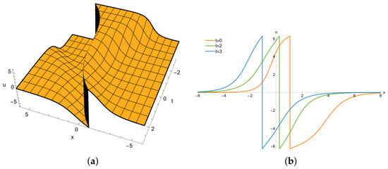
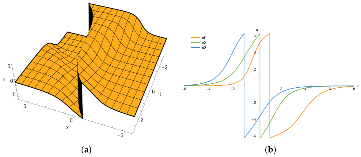
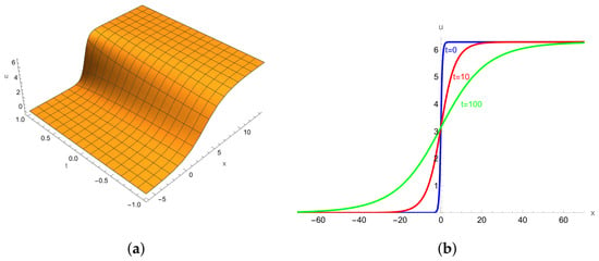
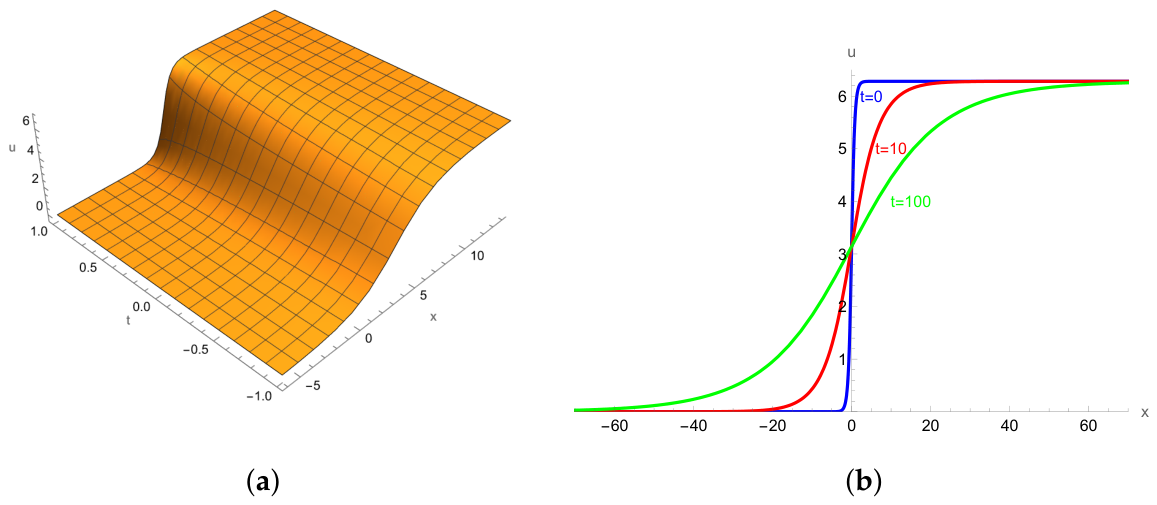
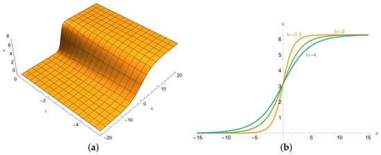
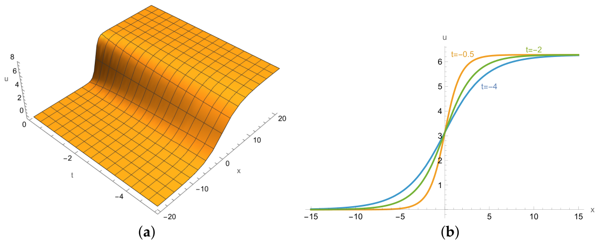
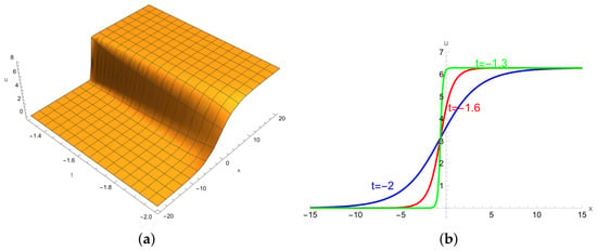
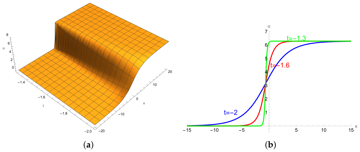
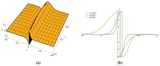
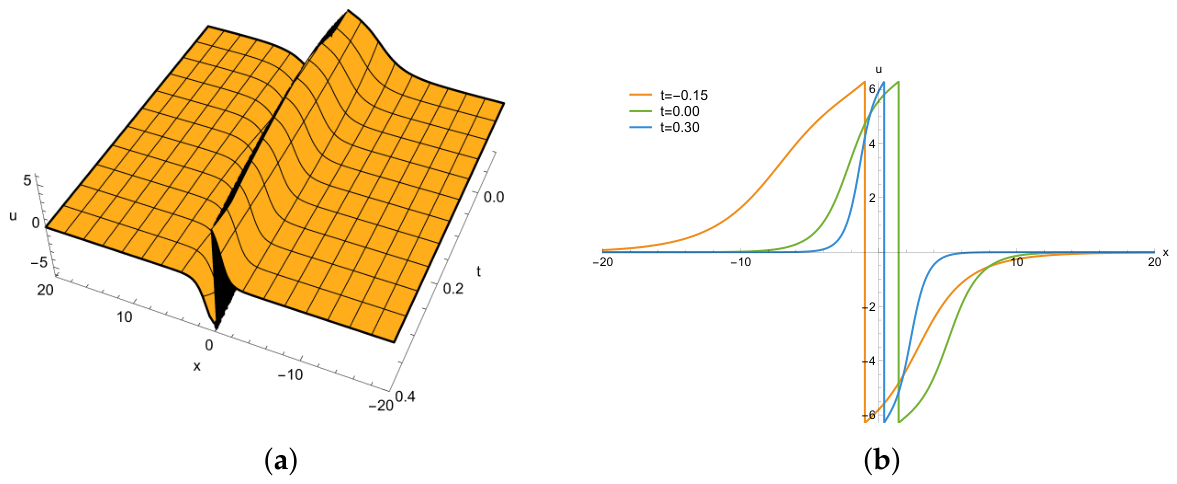
The stationary soliton can be obtained when we take ${\beta }_1\left(t\right)=-{\displaystyle \frac{1}{4c_1}}$. In this case, $x^{\prime }\left(t\right)\equiv 0$ indicates that the soliton is completely frozen in both position and shape (see Figure 1).

Figure 1. The shape of the stationary one-soliton solution (68) for $c_1=1$, ${\beta }_1\left(t\right)=-1/4$ and ${\xi }_1^{\left(0\right)}=0$. (a) 3D plot. (b) Profiles at $t=-4,-2,-0.5$.

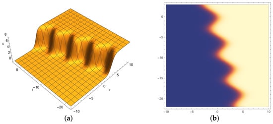
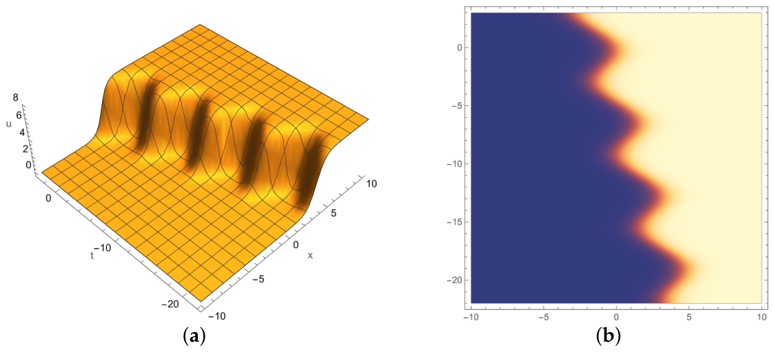
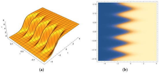
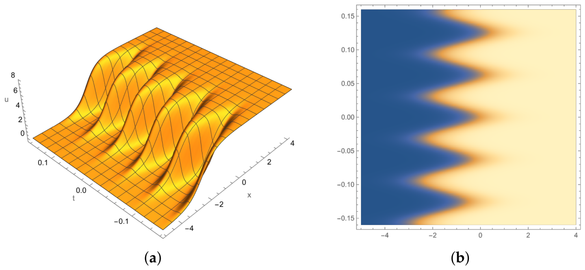
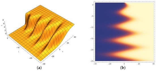
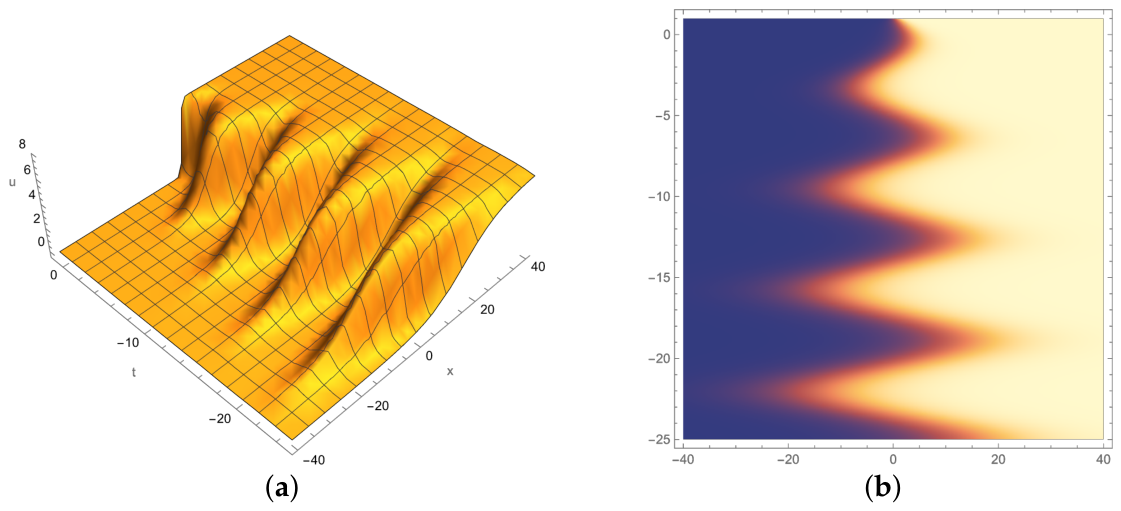
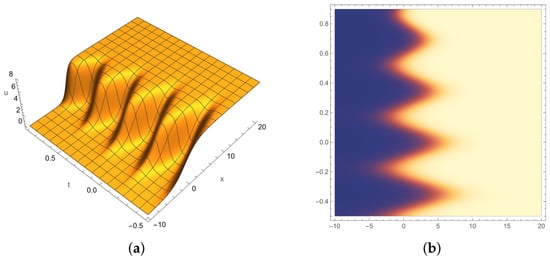
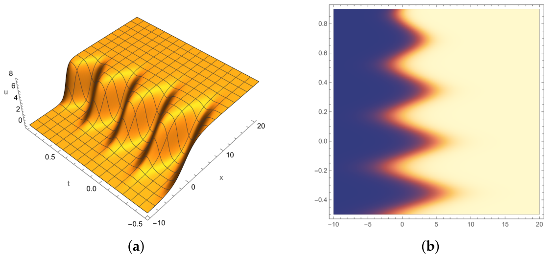
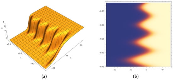
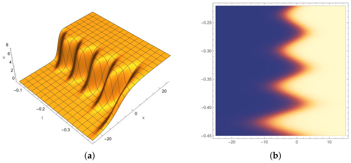
For ${\beta }_1\left(t\right)\ne -{\displaystyle \frac{1}{4c_1}}$, one can obtain a moving soliton. In the case of ${\beta }_1\left(t\right)=sint$, one obtains the one-soliton solution

$$\begin{array}{c}\hfill u=4arctan(e^{2c_{1}x+{\displaystyle \frac{1}{2c_1}}t+2(1-cost)+2{\xi }_1^{\left(0\right)}}).\end{array}$$

(73)

The wave speed becomes

$$\begin{array}{c}\hfill {\displaystyle \frac{dx\left(t\right)}{dt}}=-{\displaystyle \frac{1}{4c_1^2}}-{\displaystyle \frac{sint}{c_1}},\end{array}$$

(74)

which oscillates with time (see Figure 2).

Figure 2. The shape of moving one-soliton solution (73) for $c_1=1$ and ${\xi }_1^{\left(0\right)}=0$. (a) 3D plot. (b) Density plot. In the density plot, the color gradient represents the value of $u(x,t)$, with blue indicating values near $u=0$, cream indicating values near $u=2\pi$, and the intermediate color band marking the region of rapid variation.

We next investigate the two-soliton solution for the sG-SCS Equation (4) by means of an asymptotic analysis in terms of the phase variables. Taking $N=2$ in (59) and substituting the four possible choices $({\rho }_1,{\rho }_2)=(0,0),(1,0),(0,1),(1,1)$ into (59), one obtains

$$\begin{array}{c}\hfill f=1+i{e}^{2{\xi }_1}+i{e}^{2{\xi }_2}-e^{2{\xi }_1+2{\xi }_2+A_{12}},\end{array}$$

(75)

where

$$\begin{array}{c}\hfill e^{A_{12}}={\left({\displaystyle \frac{c_1-c_2}{c_1+c_2}}\right)}^2.\end{array}$$

(76)

Therefore, by (30), we have

$$\begin{array}{c}\hfill u(x,t)=4arctan\left({\displaystyle \frac{e^{2{\xi }_1}+e^{2{\xi }_2}}{1-e^{2({\xi }_1+{\xi }_2)+A_{12}}}}\right).\end{array}$$

(77)

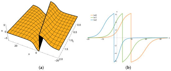
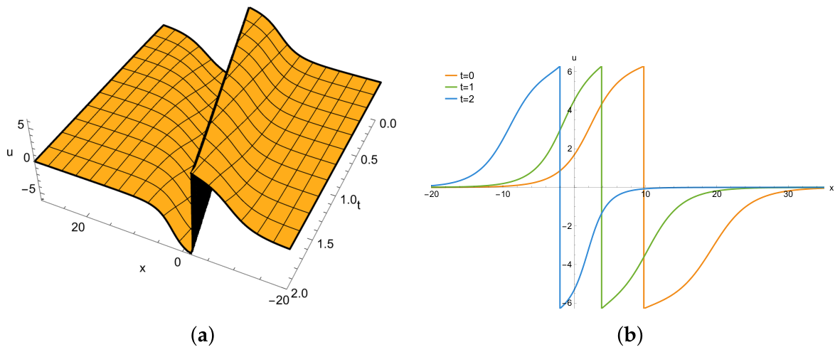
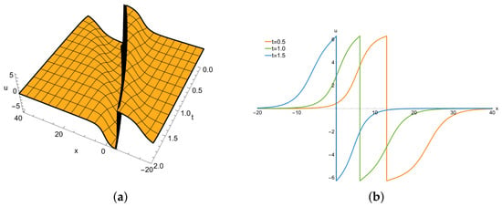
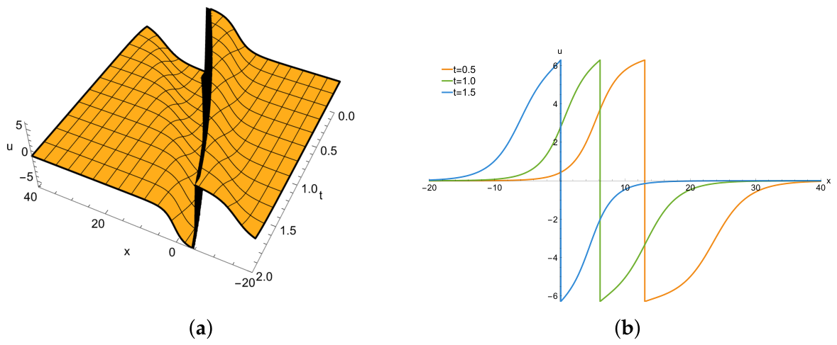
For the non-degenerate case, there exists elastic scattering between two solitons (see Figure 3).

Figure 3. The profiles of the non-degenerate solution given by (77) for $c_1=1$, $c_2=0.5$, ${\beta }_1\left(t\right)=-{\displaystyle \frac{1}{4}}+0.6e^{0.6t}$, ${\beta }_2\left(t\right)=-{\displaystyle \frac{1}{2}}+0.6e^{-0.6t}$, and ${\xi }_1^{\left(0\right)}={\xi }_2^{\left(0\right)}=0$. (a) 3D plot. (b) Profiles at $t=0,1,2$.

For the degenerate case, we take $c_1=c_2=c>0$. Then, $e^{A_{12}}=0$ and (77) reduces to the degenerate solution

$$\begin{array}{c}\hfill u(x,t)=4arctan(e^{2{\xi }_1}+e^{2{\xi }_2}),\end{array}$$

(78)

where

$$\begin{array}{c}\hfill {\xi }_j=cx+{\displaystyle \frac{t}{4c}}+{\int }_0^t{\beta }_j\left(z\right)dz+{\xi }_j^{\left(0\right)},j=1,2.\end{array}$$

(79)

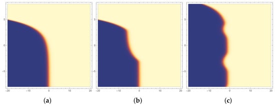
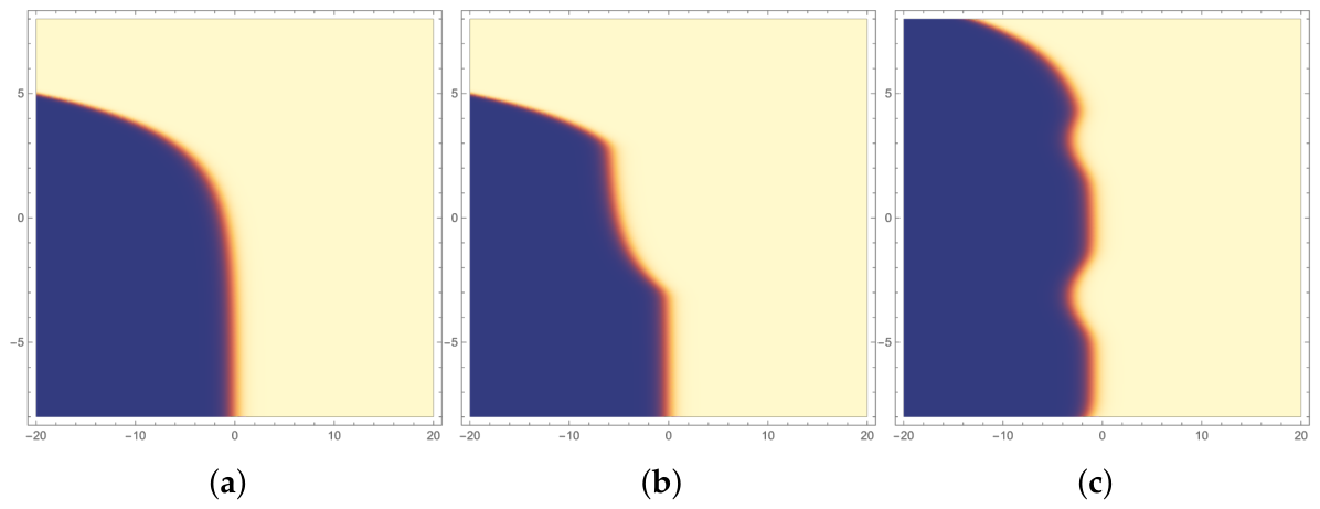
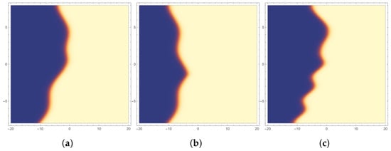
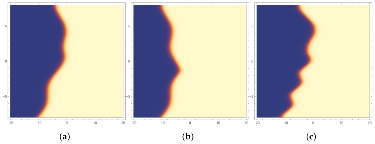
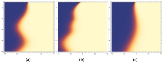
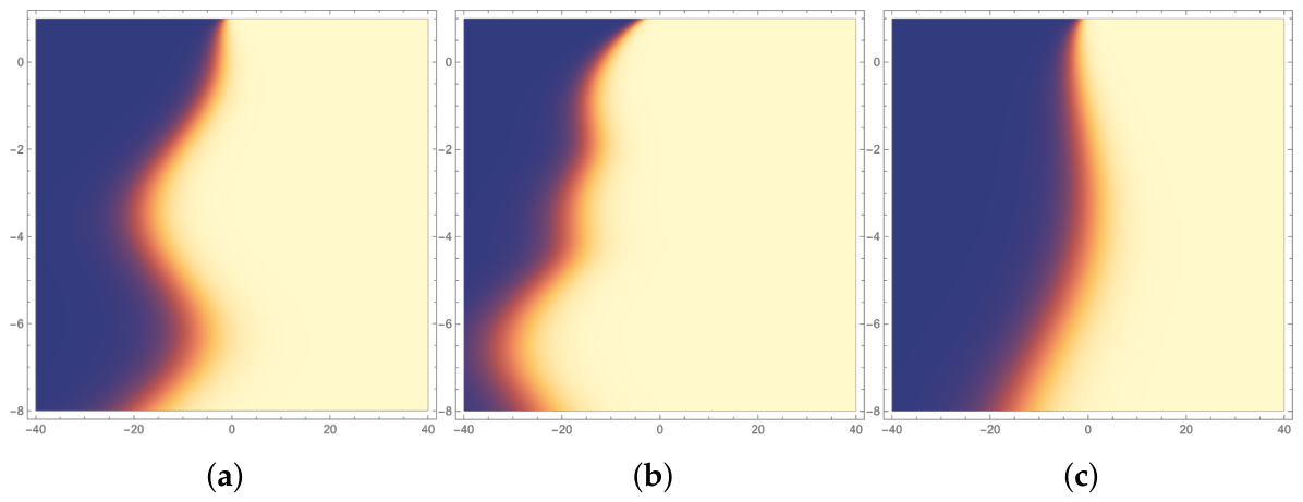
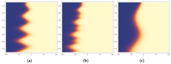
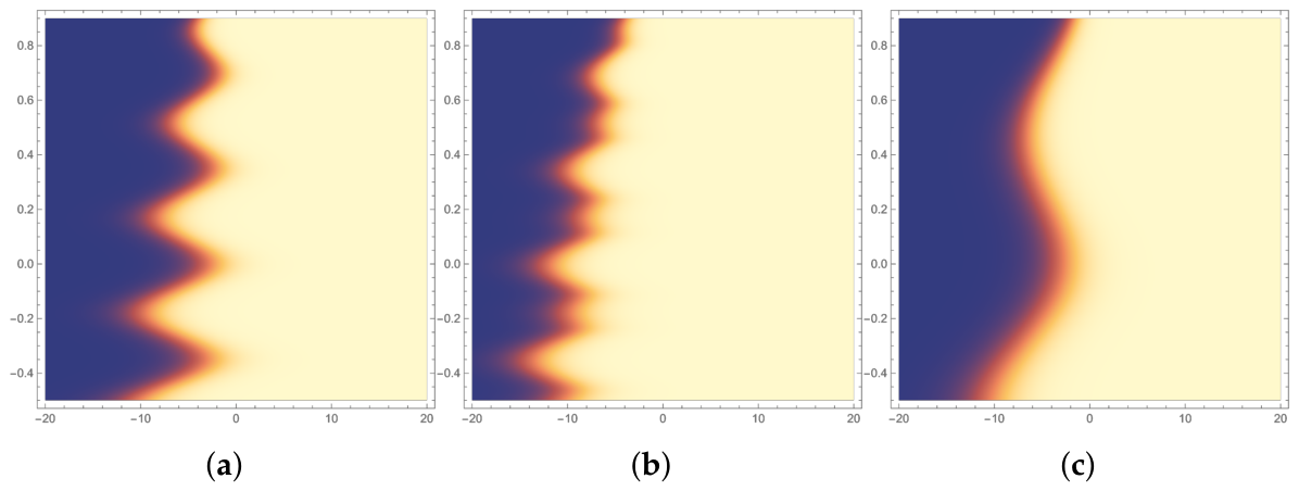
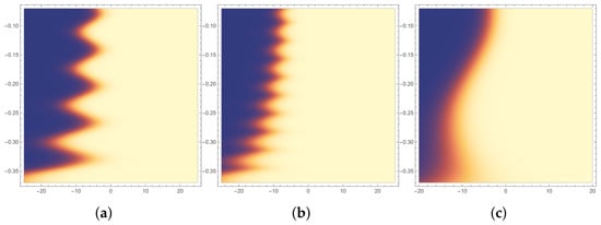
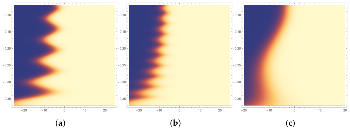
Figure 4a–c show the density plots of the degenerate two-soliton solution (78) for the basic configuration, the modified initial phases, and the modified source functions, respectively. We call the disappearing branch a “ghost” soliton because, although it appears in the explicit Formula (78), it cannot be seen in the density plot at large times. Only the surviving soliton is visible, but its trajectory still feels the presence of the ghost through the phase difference ${\int }_0^t({\beta }_1-{\beta }_2)dz$. The plots illustrate the ghost-soliton disturbance and the source-induced change in the soliton trajectory.

Figure 4. The density plots of the degenerate solution given by (78) for $c=1$. (a) The basic configuration with ${\beta }_1\left(t\right)=-{\displaystyle \frac{1}{4}}+0.6e^{0.6t}$, ${\beta }_2\left(t\right)=-{\displaystyle \frac{1}{4}}+0.6e^{-0.6t}$, ${\xi }_1^{\left(0\right)}=1$, and ${\xi }_2^{\left(0\right)}=-1$. (b) The case with modified initial phases ${\xi }_1^{\left(0\right)}=1$ and ${\xi }_2^{\left(0\right)}=5$, while ${\beta }_1\left(t\right)=-{\displaystyle \frac{1}{4}}+0.6e^{0.6t}$ and ${\beta }_2\left(t\right)=-{\displaystyle \frac{1}{4}}+0.6e^{-0.6t}$ remain unchanged. (c) The case with modified source functions ${\beta }_1\left(t\right)=-{\displaystyle \frac{1}{4}}+0.06e^{0.6t}$ and ${\beta }_2\left(t\right)=-{\displaystyle \frac{1}{4}}+2sint$, with ${\xi }_1^{\left(0\right)}=1$ and ${\xi }_2^{\left(0\right)}=-1$. The plots show that a soliton is disturbed by another invisible “ghost” soliton, and that the source variation changes the soliton trajectory. In the density plot, the color gradient represents the value of $u(x,t)$, with blue indicating values near $u=0$, cream indicating values near $u=2\pi$, and the intermediate color band marking the region of rapid variation.

Finally, we analyze the long-time asymptotic behavior of the degenerate solution (78). Suppose that $\left\{{\beta }_j\left(t\right)\right\}$ satisfies

$$\begin{array}{c}\hfill {\int }_0^t\left({\beta }_1\left(z\right)-{\beta }_2\left(z\right)\right)dz\to -\infty ,t\to +\infty .\end{array}$$

(80)

Consider first the co-moving coordinate associated with the ${\xi }_1$-soliton, namely ${\xi }_1=0$. From (79), the phase difference is

$$\begin{array}{c}\hfill {\xi }_2-{\xi }_1={\int }_0^t\left({\beta }_2\left(z\right)-{\beta }_1\left(z\right)\right)dz+{\xi }_2^{\left(0\right)}-{\xi }_1^{\left(0\right)}.\end{array}$$

(81)

Since condition (80) is equivalent to

$${\int }_0^t\left({\beta }_2\left(z\right)-{\beta }_1\left(z\right)\right)dz\to +\infty ,t\to +\infty ,$$

it follows from (81) that

$$\begin{array}{c}\hfill {\xi }_2-{\xi }_1\to +\infty ,t\to +\infty .\end{array}$$

(82)

Hence, along the trajectory ${\xi }_1=0$, we have

$$\begin{array}{c}\hfill {\xi }_2\to +\infty ,t\to +\infty .\end{array}$$

(83)

Substituting this into (78), we recognize

$$\begin{array}{c}\hfill u(x,t)=4arctan(e^{2{\xi }_1}+e^{2{\xi }_2})\to 2\pi ,t\to +\infty .\end{array}$$

(84)

This shows that, in the co-moving coordinate of the ${\xi }_1$-soliton, the solution tends to a vacuum state. Here, $u=2\pi$ is equivalent to $u=0$ as a vacuum state of the sG equation.

Next, consider the co-moving coordinate associated with the ${\xi }_2$-soliton, namely ${\xi }_2=0$. Then, from (79), we have

$$\begin{array}{c}\hfill {\xi }_1-{\xi }_2={\int }_0^t\left({\beta }_1\left(z\right)-{\beta }_2\left(z\right)\right)dz+{\xi }_1^{\left(0\right)}-{\xi }_2^{\left(0\right)}.\end{array}$$

(85)

By (80), it follows that

$$\begin{array}{c}\hfill {\xi }_1\to -\infty ,t\to +\infty .\end{array}$$

(86)

Therefore,

$$\begin{array}{c}\hfill e^{2{\xi }_1}\to 0,t\to +\infty ,\end{array}$$

(87)

and (78) yields

$$\begin{array}{c}\hfill u(x,t)=4arctan(e^{2{\xi }_1}+e^{2{\xi }_2})\to 4arctan{e}^{2{\xi }_2},t\to +\infty .\end{array}$$

(88)

Thus, the local profile tends to a single surviving soliton described by ${\xi }_2$.

Consequently, under condition (80), the ${\xi }_1$-soliton disappears asymptotically, while the ${\xi }_2$-soliton survives. Obviously, the opposite conclusion holds under the condition

$$\begin{array}{c}\hfill {\int }_0^t\left({\beta }_1\left(z\right)-{\beta }_2\left(z\right)\right)dz\to +\infty ,t\to +\infty .\end{array}$$

(89)

(II). If ${\mu }_2={\mu }_3={\nu }_2=0$, Equation (2) reduces to the mKdV-sG-SCS Equation (5). In this situation, $\left\{{\xi }_j\right\}$ in (38) read

$$\begin{array}{c}\hfill {\xi }_j=c_{j}x+\left(-4{\mu }_1{c}_j^3+{\displaystyle \frac{{\nu }_1}{4c_j}}\right)t+{\int }_0^t{\beta }_j\left(z\right)dz+{\xi }_j^{\left(0\right)},\end{array}$$

(90)

and the one-soliton solution takes the form

$$\begin{array}{c}\hfill u=4arctan{e}^{2{\xi }_1},\end{array}$$

(91)

with sources

$$\begin{array}{c}\hfill {\varphi }_{11}=\sqrt{{\beta }_1\left(t\right)}{e}^{-{\xi }_1}sech2{\xi }_1,{\varphi }_{21}=-\sqrt{{\beta }_1\left(t\right)}{e}^{{\xi }_1}sech2{\xi }_1.\end{array}$$

(92)

This is again a kink soliton with wave span $2\pi$. The inflexion point is expressed as

$$\begin{array}{c}\hfill \left(x=\left(4{\mu }_1{c}_1^2-{\displaystyle \frac{{\nu }_1}{4c_1^2}}\right)t-{\displaystyle \frac{1}{c_1}}{\int }_0^t{\beta }_1\left(z\right)dz-{\displaystyle \frac{{\xi }_1^{\left(0\right)}}{c_1}},t\right),\end{array}$$

(93)

at which $u\equiv \pi$. The wave speed reads

$$\begin{array}{c}\hfill {\displaystyle \frac{dx\left(t\right)}{dt}}=4{\mu }_1{c}_1^2-{\displaystyle \frac{{\nu }_1}{4c_1^2}}-{\displaystyle \frac{{\beta }_1\left(t\right)}{c_1}},\end{array}$$

(94)

and the slope at the inflexion point is

$$\begin{array}{c}\hfill {\displaystyle \frac{du(x,t)}{dx}}=4c_1.\end{array}$$

(95)

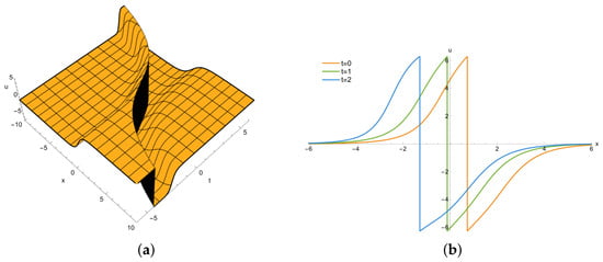
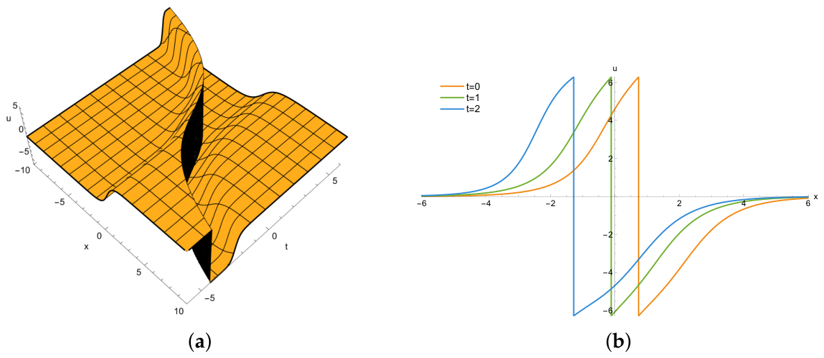
The background wave speed $4{\mu }_1{c}_1^2-{\displaystyle \frac{{\nu }_1}{4c_1^2}}$ is now controlled jointly by parameters ${\mu }_1$ and ${\nu }_1$. Setting ${\mu }_1=0$ and ${\nu }_1=1$ recovers Case (I). The stationary soliton is obtained by taking ${\beta }_1\left(t\right)=4{\mu }_1{c}_1^3-{\displaystyle \frac{{\nu }_1}{4c_1}}$ (see Figure 5).

Figure 5. The shape of the stationary one-soliton solution (91) for $c_1=1$, ${\mu }_1=1$, ${\nu }_1=1$, ${\beta }_1\left(t\right)=15/4$ and ${\xi }_1^{\left(0\right)}=0$. (a) 3D plot. (b) Profiles at $t=-4,-2,-0.5$.

Taking ${\beta }_1\left(t\right)=100sin100t$ gives a moving soliton. In this case,

$$\begin{array}{c}\hfill u=4arctan\left(e^{2c_{1}x+2\left(-4{\mu }_1{c}_1^3+{\displaystyle \frac{{\nu }_1}{4c_1}}\right)t+2(1-cos100t)+2{\xi }_1^{\left(0\right)}}\right).\end{array}$$

(96)

The wave speed becomes

$$\begin{array}{c}\hfill {\displaystyle \frac{dx}{dt}}=-{\displaystyle \frac{100sin100t}{c_1}}+4{\mu }_1{c}_1^2-{\displaystyle \frac{{\nu }_1}{4c_1^2}},\end{array}$$

(97)

which oscillates periodically about the background speed $4{\mu }_1{c}_1^2-{\displaystyle \frac{{\nu }_1}{4c_1^2}}$ (see Figure 6).

Figure 6. The shape of the moving one-soliton solution (96) for $c_1=1$, ${\mu }_1=1$, ${\nu }_1=1$ and ${\xi }_1^{\left(0\right)}=0$. (a) 3D plot. (b) Density plot. In the density plot, the color gradient represents the value of $u(x,t)$, with blue indicating values near $u=0$, cream indicating values near $u=2\pi$, and the intermediate color band marking the region of rapid variation.

The two-soliton solution for mKdV-sG-SCS Equation (5) is of the form

$$\begin{array}{c}\hfill u(x,t)=4arctan\left({\displaystyle \frac{e^{2{\xi }_1}+e^{2{\xi }_2}}{1-e^{2({\xi }_1+{\xi }_2)+A_{12}}}}\right),\end{array}$$

(98)

where $e^{A_{12}}$ is given by (76) and $\left\{{\xi }_j\right\}$ are determined by (90).

For the non-degenerate case, there exists elastic scattering between two solitons (see Figure 7).

Figure 7. The profiles of the non-degenerate solution given by (98) for $c_1=1$, $c_2=0.5$, ${\mu }_1=1$, ${\nu }_1=1$, ${\beta }_1\left(t\right)=2.55+0.6e^{0.6t}$, ${\beta }_2\left(t\right)=0.3+0.6e^{-0.6t}$, ${\xi }_1^{\left(0\right)}=0.3$, and ${\xi }_2^{\left(0\right)}=-0.8$. (a) 3D plot. (b) Profiles at $t=0,2,3$.

For the degenerate case $c_1=c_2=c>0$, one obtains $e^{A_{12}}=0$, and (98) reduces to the degenerate solution

$$\begin{array}{c}\hfill u(x,t)=4arctan(e^{2{\xi }_1}+e^{2{\xi }_2}),\end{array}$$

(99)

where

$$\begin{array}{c}\hfill {\xi }_j=cx+\left(-4{\mu }_1{c}^3+{\displaystyle \frac{{\nu }_1}{4c}}\right)t+{\int }_0^t{\beta }_j\left(z\right)dz+{\xi }_j^{\left(0\right)},j=1,2.\end{array}$$

(100)

Figure 8a–c show the density plots of the degenerate two-soliton solution for the basic configuration, the modified initial phases, and the modified source functions, respectively. The plots show that a soliton is disturbed by another invisible “ghost” soliton, and that the source variation changes the soliton’s trajectory.

Figure 8. The density plots of the degenerate solution given by (99) for $c=1$, ${\mu }_1=1$, and ${\nu }_1=1$. (a) The basic configuration with ${\beta }_1\left(t\right)={\displaystyle \frac{11}{4}}+sint$ and ${\beta }_2\left(t\right)={\displaystyle \frac{17}{4}}+cost$, where ${\xi }_1^{\left(0\right)}=1$ and ${\xi }_2^{\left(0\right)}=-1$. (b) The case with modified initial phases ${\xi }_1^{\left(0\right)}=1$ and ${\xi }_2^{\left(0\right)}=5$, while the source functions remain unchanged. (c) The case with modified source functions ${\beta }_1\left(t\right)={\displaystyle \frac{11}{4}}+2sin\left(2t\right)$ and ${\beta }_2\left(t\right)={\displaystyle \frac{17}{4}}+2cost$, with ${\xi }_1^{\left(0\right)}=1$ and ${\xi }_2^{\left(0\right)}=-1$. In the density plot, the color gradient represents the value of $u(x,t)$, with blue indicating values near $u=0$, cream indicating values near $u=2\pi$, and the intermediate color band marking the region of rapid variation.

Finally, we analyze the asymptotic behavior of the degenerate solution (99). From (100), the phase difference is

$$\begin{array}{c}\hfill {\xi }_2-{\xi }_1={\int }_0^t\left({\beta }_2\left(z\right)-{\beta }_1\left(z\right)\right)dz+{\xi }_2^{\left(0\right)}-{\xi }_1^{\left(0\right)},\end{array}$$

(101)

which has the same form as in Case (I). Suppose $\left\{{\beta }_j\left(t\right)\right\}$ satisfy (80). Then, in the co-moving coordinate associated with the ${\xi }_1$-soliton, setting ${\xi }_1=0$ gives rise to

$$\begin{array}{c}\hfill {\xi }_2={\int }_0^t\left({\beta }_2\left(z\right)-{\beta }_1\left(z\right)\right)dz+{\xi }_2^{\left(0\right)}-{\xi }_1^{\left(0\right)}\to +\infty ,t\to +\infty ,\end{array}$$

(102)

and thus

$$\begin{array}{c}\hfill u\to 2\pi ,t\to +\infty .\end{array}$$

(103)

Similarly, in the co-moving coordinate associated with the ${\xi }_2$-soliton, setting ${\xi }_2=0$ yields

$$\begin{array}{c}\hfill {\xi }_1={\int }_0^t\left({\beta }_1\left(z\right)-{\beta }_2\left(z\right)\right)dz+{\xi }_1^{\left(0\right)}-{\xi }_2^{\left(0\right)}\to -\infty ,t\to +\infty ,\end{array}$$

(104)

hence

$$\begin{array}{c}\hfill u(x,t)\to 4arctan{e}^{2{\xi }_2},t\to +\infty ,\end{array}$$

(105)

which indicates that the ${\xi }_1$-soliton disappears in this limit. Note that $u=2\pi$ is equivalent to $u=0$ as a vacuum state of the sG equation, since $sin\left(2\pi \right)=sin\left(0\right)=0$. Therefore, under condition (80), in the degenerate case the ${\xi }_1$-soliton disappears, while the ${\xi }_2$-soliton survives. Obviously, the opposite conclusion holds under condition (89).

(III). If ${\mu }_1={\mu }_2={\nu }_1={\nu }_2=0$ and ${\mu }_3=1$, we obtain the ni-mKdV-SCSs (6). $\left\{{\xi }_j\right\}$ in this case read

$$\begin{array}{c}\hfill {\xi }_j={\displaystyle \frac{x}{\sqrt{-8t+c_j}}}-{\displaystyle \frac{1}{2}}ln(-8t+c_j)+{\int }_0^t{\beta }_j\left(z\right)dz+{\xi }_j^{\left(0\right)}.\end{array}$$

(106)

The one-soliton solution takes the form

$$\begin{array}{c}\hfill u=4arctan\left({\displaystyle \frac{1}{c_1-8t}}{e}^{{\displaystyle \frac{2}{\sqrt{c_1-8t}}}x+2{\int }_0^t{\beta }_1\left(z\right)dz+2{\xi }_1^{\left(0\right)}}\right)\end{array}$$

(107)

with sources

$$\begin{array}{c}\hfill {\varphi }_{11}=\sqrt{{\beta }_1\left(t\right)}{e}^{-{\xi }_1}sech2{\xi }_1,{\varphi }_{21}=-\sqrt{{\beta }_1\left(t\right)}{e}^{{\xi }_1}sech2{\xi }_1.\end{array}$$

(108)

This is a kink soliton with wave span $2\pi$. We note that solution (107) is well-defined only for $t<c_1/8$, since $k_1\left(t\right)=1/\sqrt{c_1-8t}$ blows up as $t\to {(c_1/8)}^{-}$. In the multisoliton case, the validity is correspondingly restricted to $t<{min}_j(c_j/8)$. We can describe nonisospectral behaviors through the time-dependent speed and slope of the inflexion point

$$\begin{array}{c}\hfill \left(x={\displaystyle \frac{\sqrt{c_1-8t}}{2}}\left(ln(c_1-8t)-2{\int }_0^t{\beta }_1\left(z\right)dz-2{\xi }_1^{\left(0\right)}\right),t\right),\end{array}$$

(109)

at which $u\equiv \pi$. The speed is

$$\begin{array}{c}\hfill {\displaystyle \frac{dx\left(t\right)}{dt}}={\displaystyle \frac{-2\left(ln(c_1-8t)-2{\int }_0^t{\beta }_1\left(z\right)dz-2{\xi }_1^{\left(0\right)}+2\right)}{\sqrt{c_1-8t}}}-\sqrt{c_1-8t}{\beta }_1\left(t\right),\end{array}$$

(110)

and the slope of the wave at the inflexion point reads

$$\begin{array}{c}\hfill {\displaystyle \frac{du(x,t)}{dx}}={\displaystyle \frac{4}{\sqrt{c_1-8t}}}.\end{array}$$

(111)

When

$$\begin{array}{c}\hfill {\beta }_1\left(t\right)=-{\displaystyle \frac{4}{c_1-8t}}+{\displaystyle \frac{2\sqrt{c_1}(2{\xi }_1^{\left(0\right)}-ln{c}_1)}{{(c_1-8t)}^{3/2}}},\end{array}$$

(112)

we obtain the stationary wave (see Figure 9).

Figure 9. The shape of the stationary one-soliton solution (107) for $c_1=9$, ${\xi }_1^{\left(0\right)}=0$ and ${\beta }_1\left(t\right)$ as in (112). (a) 3D plot. (b) Profiles at $t=0,10,100$.

Taking ${\beta }_1\left(t\right)=-{\displaystyle \frac{4}{c_1-8t}}+sint$ gives rise to a moving soliton solution

$$\begin{array}{c}\hfill u=4arctan\left({\displaystyle \frac{1}{c_1}}{e}^{{\displaystyle \frac{2}{\sqrt{c_1-8t}}}x+2(1-cost)+2{\xi }_1^{\left(0\right)}}\right).\end{array}$$

(113)

This case exhibits richer dynamics than Cases (I) and (II), since the source $sint$ drives oscillatory motion of the soliton, while the wave profile becomes narrower and steeper due to the nonisospectral effect (see Figure 10).

Figure 10. The shape of the moving one-soliton solution (113) for $c_1=9$ and ${\xi }_1^{\left(0\right)}=0$. (a) 3D plot. (b) Density plot. In the density plot, the color gradient represents the value of $u(x,t)$, with blue indicating values near $u=0$, cream indicating values near $u=2\pi$, and the intermediate color band marking the region of rapid variation.

Unlike Cases (I) and (II), where $\{k_j\left(t\right)=c_j\}$ are constants, here $\left\{k_j\left(t\right)\right\}$ are time-dependent; thus, the interaction coefficient

$$\begin{array}{c}\hfill e^{A_{12}}={\left({\displaystyle \frac{k_1\left(t\right)-k_2\left(t\right)}{k_1\left(t\right)+k_2\left(t\right)}}\right)}^2={\left({\displaystyle \frac{\sqrt{-8t+c_2}-\sqrt{-8t+c_1}}{\sqrt{-8t+c_2}+\sqrt{-8t+c_1}}}\right)}^2\end{array}$$

(114)

is also time-dependent, and the two-soliton solution is

$$\begin{array}{c}\hfill u(x,t)=4arctan\left({\displaystyle \frac{e^{2{\xi }_1}+e^{2{\xi }_2}}{1-e^{2({\xi }_1+{\xi }_2)+A_{12}}}}\right).\end{array}$$

(115)

With regards to the non-degenerate case $c_1\ne c_2$, there exists an elastic-type interaction between two solitons on a nonisospectral background (see Figure 11).

Figure 11. The profiles of the non-degenerate solution given by (115) for $c_1=49$, $c_2=25$, ${\mu }_3=1$, ${\beta }_1\left(t\right)=0.6e^{0.6t}$, ${\beta }_2\left(t\right)=0.6e^{-0.6t}$, ${\xi }_1^{\left(0\right)}=1$, and ${\xi }_2^{\left(0\right)}=1$. (a) 3D plot. (b) Profiles at $t=0,1,2$.

When $c_1=c_2=c>0$, one obtains $k_1\left(t\right)=k_2\left(t\right)$. Hence, $e^{A_{12}}=0$, and (115) reduces to the degenerate solution

$$\begin{array}{c}\hfill u(x,t)=4arctan(e^{2{\xi }_1}+e^{2{\xi }_2}),\end{array}$$

(116)

where

$$\begin{array}{c}\hfill {\xi }_j={\displaystyle \frac{x}{\sqrt{-8t+c}}}-{\displaystyle \frac{1}{2}}ln(-8t+c)+{\int }_0^t{\beta }_j\left(z\right)dz+{\xi }_j^{\left(0\right)},j=1,2.\end{array}$$

(117)

Figure 12a–c show the density plots of the degenerate two-soliton solution for the basic configuration, the modified initial phases, and the modified source functions, respectively. The plots show the ghost-soliton disturbance on a nonisospectral background, together with the time-dependent deformation of the profile.

Figure 12. The density plots of the degenerate solution given by (116) for $c=9$. (a) The basic configuration with ${\beta }_1\left(t\right)=-{\displaystyle \frac{4}{c-8t}}+sint$ and ${\beta }_2\left(t\right)=-{\displaystyle \frac{4}{c-8t}}-sint$, where ${\xi }_1^{\left(0\right)}=2$ and ${\xi }_2^{\left(0\right)}=-2$. (b) The case with modified initial phases ${\xi }_1^{\left(0\right)}=2$ and ${\xi }_2^{\left(0\right)}=5$, while the source functions remain unchanged. (c) The case with modified source functions ${\beta }_1\left(t\right)=-{\displaystyle \frac{4}{c-8t}}+0.5cos\left(0.5t\right)$ and ${\beta }_2\left(t\right)=-{\displaystyle \frac{4}{c-8t}}-0.5cos\left(0.5t\right)$, with ${\xi }_1^{\left(0\right)}=2$ and ${\xi }_2^{\left(0\right)}=-2$. The plots illustrate the ghost-soliton disturbance and the source-controlled deformation of the propagation pattern. In the density plot, the color gradient represents the value of $u(x,t)$, with blue indicating values near $u=0$, cream indicating values near $u=2\pi$, and the intermediate color band marking the region of rapid variation.

We conclude by analyzing the asymptotic behavior of the degenerate solution (116). From (117), the phase difference is

$$\begin{array}{c}\hfill {\xi }_2-{\xi }_1={\int }_0^t\left({\beta }_2\left(z\right)-{\beta }_1\left(z\right)\right)dz+{\xi }_2^{\left(0\right)}-{\xi }_1^{\left(0\right)},\end{array}$$

(118)

since the nonisospectral terms ${\displaystyle \frac{x}{\sqrt{-8t+c}}}$ and $-{\displaystyle \frac{1}{2}}ln(-8t+c)$ cancel out in the difference, where $c=c_1=c_2$. Suppose that $\left\{{\beta }_j\left(t\right)\right\}$ satisfy

$$\begin{array}{c}\hfill {\int }_0^t\left({\beta }_1\left(z\right)-{\beta }_2\left(z\right)\right)dz\to -\infty ,t\to {\left({\displaystyle \frac{c}{8}}\right)}^{-}.\end{array}$$

(119)

Then, in the co-moving coordinate associated with the ${\xi }_1$-soliton, setting ${\xi }_1=0$ implies

$$\begin{array}{c}\hfill {\xi }_2={\int }_0^t\left({\beta }_2\left(z\right)-{\beta }_1\left(z\right)\right)dz+{\xi }_2^{\left(0\right)}-{\xi }_1^{\left(0\right)}\to +\infty ,t\to {\left({\displaystyle \frac{c}{8}}\right)}^{-};\end{array}$$

(120)

hence,

$$\begin{array}{c}\hfill u\to 2\pi ,t\to {\left({\displaystyle \frac{c}{8}}\right)}^{-}.\end{array}$$

(121)

Similarly, in the co-moving coordinate associated with the ${\xi }_2$-soliton, setting ${\xi }_2=0$ results in

$$\begin{array}{c}\hfill {\xi }_1={\int }_0^t\left({\beta }_1\left(z\right)-{\beta }_2\left(z\right)\right)dz+{\xi }_1^{\left(0\right)}-{\xi }_2^{\left(0\right)}\to -\infty ,t\to {\left({\displaystyle \frac{c}{8}}\right)}^{-};\end{array}$$

(122)

hence,

$$\begin{array}{c}\hfill u(x,t)\to 4arctan{e}^{2{\xi }_2},t\to {\left({\displaystyle \frac{c}{8}}\right)}^{-}.\end{array}$$

(123)

Therefore, under condition (119), the ${\xi }_1$-soliton disappears, while the ${\xi }_2$-soliton survives. Obviously, the opposite conclusion holds under the condition

$$\begin{array}{c}\hfill {\int }_0^t\left({\beta }_1\left(z\right)-{\beta }_2\left(z\right)\right)dz\to +\infty ,t\to {\left({\displaystyle \frac{c}{8}}\right)}^{-}.\end{array}$$

(124)

(IV). If ${\mu }_1={\mu }_2={\nu }_2=0,{\mu }_3={\nu }_1=1$, we obtain a nonisospectral equation with SCSs

$$\begin{array}{cc}\hfill & u_{tx}=x\left(u_{xxxx}+{\displaystyle \frac{3}{2}}{u}_x^2{u}_{xx}\right)+3u_{xxx}+u_x^3+{\displaystyle \frac{1}{2}}{u}_{xx}{\partial }^{-1}{u}_x^2+sinu+2{\displaystyle \sum _{j=1}^N}{({\varphi }_{1j}^2+{\varphi }_{2j}^2)}_x,\hfill \end{array}$$

(125)

$$\begin{array}{cc}\hfill & {\varphi }_{1j,x}=-{\lambda }_j\left(t\right){\varphi }_{1j}+{\displaystyle \frac{u_x}{2}}{\varphi }_{2j},{\varphi }_{2j,x}=-{\displaystyle \frac{u_x}{2}}{\varphi }_{1j}+{\lambda }_j\left(t\right){\varphi }_{2j},(j=1,2,\dots ,N),\hfill \end{array}$$

(126)

where $\{{\lambda }_j={\lambda }_j\left(t\right)\}$ are N different time-dependent eigenvalues. Introduce $\left\{{\xi }_j\right\}$ as

$$\begin{array}{c}\hfill {\xi }_j={\displaystyle \frac{x}{\sqrt{c_j-8t}}}-{\displaystyle \frac{1}{48}}{(-8t+c_j)}^{{\displaystyle \frac{3}{2}}}-{\displaystyle \frac{1}{2}}ln(-8t+c_j)+{\int }_0^t{\beta }_j\left(z\right)dz+{\xi }_j^{\left(0\right)}.\end{array}$$

(127)

Then, one can write down the one-soliton solution

$$\begin{array}{c}\hfill u=4arctan\left({\displaystyle \frac{1}{c_1-8t}}{e}^{{\displaystyle \frac{2}{\sqrt{c_1-8t}}}x-{\displaystyle \frac{1}{24}}{(c_1-8t)}^{{\displaystyle \frac{3}{2}}}+2{\int }_0^t{\beta }_1\left(z\right)dz+2{\xi }_1^{\left(0\right)}}\right),\end{array}$$

(128)

with the corresponding sources

$$\begin{array}{c}\hfill {\varphi }_{11}=\sqrt{{\beta }_1\left(t\right)}{e}^{-{\xi }_1}sech2{\xi }_1,{\varphi }_{21}=-\sqrt{{\beta }_1\left(t\right)}{e}^{{\xi }_1}sech2{\xi }_1.\end{array}$$

(129)

Solution (128) is a kink soliton with wave span $2\pi$. The value of u at the inflexion point

$$\begin{array}{c}\hfill \left(x={\displaystyle \frac{\sqrt{c_1-8t}}{2}}\left(ln(c_1-8t)+{\displaystyle \frac{1}{24}}{(c_1-8t)}^{{\displaystyle \frac{3}{2}}}-2{\int }_0^t{\beta }_1\left(z\right)dz-2{\xi }_1^{\left(0\right)}\right),t\right)\end{array}$$

(130)

is still $\pi$. The time-dependent speed and slope of the inflexion point are

$$\begin{array}{cc}\hfill {\displaystyle \frac{dx\left(t\right)}{dt}}=& {\displaystyle \frac{1}{4\sqrt{c_1-8t}}}(-8ln(c_1-8t)-{\displaystyle \frac{4}{3}}{(c_1-8t)}^{{\displaystyle \frac{3}{2}}}-4(c_1-8t){\beta }_1\left(t\right)\hfill \\ \hfill & +16{\int }_0^t{\beta }_1\left(z\right)dz+16{\xi }_1^{\left(0\right)}-16),\hfill \end{array}$$

(131)

and

$$\begin{array}{c}\hfill {\displaystyle \frac{du(x,t)}{dx}}={\displaystyle \frac{4}{\sqrt{c_1-8t}}},\end{array}$$

(132)

respectively.

Unlike Case (III), solution (128) is only valid for $t<{\displaystyle \frac{c_1}{8}}$, since $k_1\left(t\right)={\displaystyle \frac{1}{\sqrt{c_1-8t}}}$ blows up as $t\to {\displaystyle \frac{c_1^{-}}{8}}$. The slope at the inflexion point increases with time and diverges as $t\to {\displaystyle \frac{c_1^{-}}{8}}$, meaning the soliton becomes increasingly steeper and narrower, in sharp contrast to Case (III), where the soliton broadens gradually. The real-valued function ${\beta }_1\left(t\right)$ plays the role of source and changes the velocity of the soliton, and also enters the amplitudes of the source fields through $\sqrt{{\beta }_1\left(t\right)}$. The stationary soliton can be obtained when we take the following (see Figure 13)

$$\begin{array}{c}\hfill {\beta }_1\left(t\right)={\displaystyle \frac{-c_1^2+12c_{1}t-48t^2-12\sqrt{c_1-8t}+6\sqrt{c_1}(2{\xi }_1^{\left(0\right)}-ln{c}_1)}{3{(c_1-8t)}^{3/2}}}.\end{array}$$

(133)

Figure 13. The shape of the stationary one-soliton solution given by (128) for $c_1=1$, ${\xi }_1^{\left(0\right)}=0$ and ${\beta }_1\left(t\right)$ as in (133). (a) 3D plot. (b) Profiles at $t=-4,-2,-0.5$.

Taking ${\beta }_1\left(t\right)=-{\displaystyle \frac{\sqrt{c_1-8t}}{4}}-{\displaystyle \frac{4}{c_1-8t}}+18sin18t$ gives a moving soliton solution

$$u=4arctan\left({\displaystyle \frac{1}{c_1-8t}}{e}^{{\displaystyle \frac{2}{\sqrt{c_1-8t}}}x-{\displaystyle \frac{c_1^{3/2}}{24}}-ln{c}_1+2-2cos\left(18t\right)+2{\xi }_1^{\left(0\right)}}\right).$$

(134)

The wave speed and slope both vary with time, reflecting the nonisospectral nature of this case (see Figure 14).

Figure 14. The shape of the moving one-soliton solution (134) for $c_1=9$ and ${\xi }_1^{\left(0\right)}=0$. (a) 3D plot. (b) Density plot. In the density plot, the color gradient represents the value of $u(x,t)$, with blue indicating values near $u=0$, cream indicating values near $u=2\pi$, and the intermediate color band marking the region of rapid variation.

We now turn to the two-soliton solution for the nonisospectral equation with SCSs (125), which reads

$$\begin{array}{c}\hfill u(x,t)=4arctan\left({\displaystyle \frac{e^{2{\xi }_1}+e^{2{\xi }_2}}{1-e^{2({\xi }_1+{\xi }_2)+A_{12}}}}\right)\end{array}$$

(135)

and guarantee the real property under assumption $t<min\left({\displaystyle \frac{c_1}{8}},{\displaystyle \frac{c_2}{8}}\right)$. The interaction coefficient is

$$\begin{array}{c}\hfill e^{A_{12}}={\left({\displaystyle \frac{k_1\left(t\right)-k_2\left(t\right)}{k_1\left(t\right)+k_2\left(t\right)}}\right)}^2={\left({\displaystyle \frac{\sqrt{c_2-8t}-\sqrt{c_1-8t}}{\sqrt{c_2-8t}+\sqrt{c_1-8t}}}\right)}^2.\end{array}$$

(136)

We first consider the non-degenerate case $c_1\ne c_2$ with $t<min\left({\displaystyle \frac{c_1}{8}},{\displaystyle \frac{c_2}{8}}\right)$. In this case, there exists an elastic-type interaction between two solitons on a nonisospectral background (see Figure 15).

Figure 15. The profiles of the non-degenerate solution given by (135) for $c_1=49$, $c_2=25$, ${\beta }_1\left(t\right)=0.6e^{0.6t}$, ${\beta }_2\left(t\right)=0.6e^{-0.6t}$, ${\xi }_1^{\left(0\right)}=6$, and ${\xi }_2^{\left(0\right)}=2$. (a) 3D plot. (b) Profiles at $t=0.5,1.0,1.5$.

For the degenerate case, i.e., $c_1=c_2=c$ implies $e^{A_{12}}=0$. Then, (135) reduces to the degenerate solution

$$\begin{array}{c}\hfill u(x,t)=4arctan(e^{2{\xi }_1}+e^{2{\xi }_2}),\end{array}$$

(137)

where

$$\begin{array}{c}\hfill {\xi }_j={\displaystyle \frac{x}{\sqrt{c-8t}}}-{\displaystyle \frac{1}{48}}{(-8t+c)}^{{\displaystyle \frac{3}{2}}}-{\displaystyle \frac{1}{2}}ln(-8t+c)+{\int }_0^t{\beta }_j\left(z\right)dz+{\xi }_j^{\left(0\right)},j=1,2.\end{array}$$

(138)

Figure 16a–c show the density plots of the degenerate two-soliton solution for the basic configuration, the modified initial phases, and the modified source functions, respectively. The plots show the ghost-soliton disturbance and the source-controlled deformation of the propagation pattern in a finite time interval.

Figure 16. The density plots of the degenerate solution given by (137) for $c=9$. (a) The basic configuration with ${\beta }_1\left(t\right)=-{\displaystyle \frac{4}{c-8t}}-{\displaystyle \frac{1}{4}}\sqrt{c-8t}+18sin\left(18t\right)$ and ${\beta }_2\left(t\right)=-{\displaystyle \frac{4}{c-8t}}-{\displaystyle \frac{1}{4}}\sqrt{c-8t}-18sin\left(18t\right)$, where ${\xi }_1^{\left(0\right)}=2$ and ${\xi }_2^{\left(0\right)}=-2$. (b) The case with modified initial phases ${\xi }_1^{\left(0\right)}=2$ and ${\xi }_2^{\left(0\right)}=5$, while the source functions remain unchanged. (c) The case with modified source functions ${\beta }_1\left(t\right)=-{\displaystyle \frac{4}{c-8t}}-{\displaystyle \frac{1}{4}}\sqrt{c-8t}+6sin\left(6t\right)$ and ${\beta }_2\left(t\right)=-{\displaystyle \frac{4}{c-8t}}-{\displaystyle \frac{1}{4}}\sqrt{c-8t}+2cos\left(6t\right)$, with ${\xi }_1^{\left(0\right)}=2$ and ${\xi }_2^{\left(0\right)}=-2$. The plots illustrate the ghost-soliton disturbance and the source-induced deformation of the wave profile. In the density plot, the color gradient represents the value of $u(x,t)$, with blue indicating values near $u=0$, cream indicating values near $u=2\pi$, and the intermediate color band marking the region of rapid variation.

To proceed, we analyze the asymptotic behavior of the degenerate solution (137) as $t\to {{\displaystyle \frac{c}{8}}}^{-}$. From (138), the phase difference is

$$\begin{array}{c}\hfill {\xi }_2-{\xi }_1={\int }_0^t\left({\beta }_2\left(z\right)-{\beta }_1\left(z\right)\right)dz+{\xi }_2^{\left(0\right)}-{\xi }_1^{\left(0\right)},\end{array}$$

(139)

since the nonisospectral terms ${\displaystyle \frac{x}{\sqrt{c-8t}}}$, $-{\displaystyle \frac{1}{48}}{(-8t+c)}^{{\displaystyle \frac{3}{2}}}$ and $-{\displaystyle \frac{1}{2}}ln(-8t+c)$ all cancel out in the difference. Suppose that $\left\{{\beta }_j\left(t\right)\right\}$ satisfy

$$\begin{array}{c}\hfill {\int }_0^t\left({\beta }_1\left(z\right)-{\beta }_2\left(z\right)\right)dz\to -\infty ,t\to {{\displaystyle \frac{c}{8}}}^{-},c>0.\end{array}$$

(140)

Then, in the co-moving coordinate associated with the ${\xi }_1$-soliton, setting ${\xi }_1=0$ gives

$$\begin{array}{c}\hfill {\xi }_2={\int }_0^t\left({\beta }_2\left(z\right)-{\beta }_1\left(z\right)\right)dz+{\xi }_2^{\left(0\right)}-{\xi }_1^{\left(0\right)}\to +\infty ,t\to {{\displaystyle \frac{c}{8}}}^{-};\end{array}$$

(141)

hence,

$$\begin{array}{c}\hfill u\to 2\pi ,t\to {{\displaystyle \frac{c}{8}}}^{-}.\end{array}$$

(142)

Similarly, in the co-moving coordinate associated with the ${\xi }_2$-soliton, setting ${\xi }_2=0$ affords

$$\begin{array}{c}\hfill {\xi }_1={\int }_0^t\left({\beta }_1\left(z\right)-{\beta }_2\left(z\right)\right)dz+{\xi }_1^{\left(0\right)}-{\xi }_2^{\left(0\right)}\to -\infty ,t\to {{\displaystyle \frac{c}{8}}}^{-};\end{array}$$

(143)

hence,

$$\begin{array}{c}\hfill u(x,t)\to 4arctan{e}^{2{\xi }_2},t\to {{\displaystyle \frac{c}{8}}}^{-}.\end{array}$$

(144)

Therefore, under condition (140), the ${\xi }_1$-soliton disappears, while the ${\xi }_2$-soliton survives. Obviously, the opposite conclusion holds under the condition

$$\begin{array}{c}\hfill {\int }_0^t\left({\beta }_1\left(z\right)-{\beta }_2\left(z\right)\right)dz\to +\infty ,t\to {{\displaystyle \frac{c}{8}}}^{-}.\end{array}$$

(145)

(V). If ${\mu }_1={\mu }_2={\nu }_1=0,{\mu }_3={\nu }_2=1$, we have another nonisospectral equation with SCSs

$$\begin{array}{cc}\hfill & u_{tx}=\left(x(u_{xxxx}+{\displaystyle \frac{3}{2}}{u}_x^2{u}_{xx})+3u_{xxx}+u_x^3+{\displaystyle \frac{1}{2}}{u}_{xx}{\partial }^{-1}{u}_x^2\right)\hfill \\ \hfill & +\left(xsinu-cosu{\partial }^{-1}sinu+sinu{\partial }^{-1}(cosu-1)\right)+2{\displaystyle \sum _{j=1}^N}{({\varphi }_{1j}^2+{\varphi }_{2j}^2)}_x,\hfill \end{array}$$

(146)

$$\begin{array}{cc}\hfill & {\varphi }_{1j,x}=-{\lambda }_j\left(t\right){\varphi }_{1j}+{\displaystyle \frac{u_x}{2}}{\varphi }_{2j},{\varphi }_{2j,x}=-{\displaystyle \frac{u_x}{2}}{\varphi }_{1j}+{\lambda }_j\left(t\right){\varphi }_{2j},(j=1,2,\dots ,N),\hfill \end{array}$$

(147)

where $\{{\lambda }_j={\lambda }_j\left(t\right)\}$ are N different time-dependent eigenvalues. In this case, $\left\{{\xi }_j\right\}$ become

$$\begin{array}{c}\hfill {\xi }_j={\displaystyle \frac{\sqrt{tan(2t+c_j)}}{2}}x+{\displaystyle \frac{1}{2}}ln{\displaystyle \frac{2}{sin(4t+2c_j)}}+{\int }_0^t{\beta }_j\left(z\right)dz+{\xi }_j^{\left(0\right)},\end{array}$$

(148)

which are valid on intervals where $tan(2t+c_j)>0$ and $sin(4t+2c_j)>0$. The one-soliton solution is of the form

$$\begin{array}{c}\hfill u=4arctan\left({\displaystyle \frac{2}{sin(4t+2c_1)}}{e}^{\sqrt{tan(2t+c_1)}x+2{\int }_0^t{\beta }_1\left(z\right)dz+2{\xi }_1^{\left(0\right)}}\right).\end{array}$$

(149)

The inflexion point is

$$\begin{array}{c}\hfill \left(x={\displaystyle \frac{2ln{\displaystyle \frac{sin(2c_1+4t)}{2}}-4{\int }_0^t{\beta }_1\left(z\right)dz-4{\xi }_1^{\left(0\right)}}{2\sqrt{tan(c_1+2t)}}},t\right),\end{array}$$

(150)

at which $u\equiv \pi$, the time-dependent wave speed reads

$$\begin{array}{cc}\hfill {\displaystyle \frac{dx\left(t\right)}{dt}}=& {\displaystyle \frac{{sec}^2(c_1+2t)}{{tan}^{3/2}(c_1+2t)}}(2cos(2c_1+4t)+ln{\displaystyle \frac{2}{sin(2c_1+4t)}}\hfill \\ \hfill & +2{\int }_0^t{\beta }_1\left(z\right)dz-{\beta }_1\left(t\right)sin(2c_1+4t)+2{\xi }_1^{\left(0\right)}),\hfill \end{array}$$

(151)

and the slope is described as

$$\begin{array}{c}\hfill {\displaystyle \frac{du(x,t)}{dx}}=2\sqrt{tan(2t+c_1)}.\end{array}$$

(152)

The stationary soliton (see Figure 17) can be obtained when we take

$$\begin{array}{c}\hfill {\beta }_1\left(t\right)=2cot(2c_1+4t)+{\displaystyle \frac{\left(4{\xi }_1^{\left(0\right)}+2ln{\displaystyle \frac{2}{sin\left(2c_1\right)}}\right){sec}^2(c_1+2t)}{4\sqrt{tan{c}_1}\sqrt{tan(c_1+2t)}}}.\end{array}$$

(153)

Figure 17. The shape of the stationary one-soliton solution (149) for $c_1=1$, ${\xi }_1^{\left(0\right)}=0$ and ${\beta }_1\left(t\right)$ as in (153). (a) 3D plot. (b) Profiles at $t=-2,-1.6,-1.3$.

Taking ${\beta }_1\left(t\right)=2cot(4t+2c_1)+100cos\left(100t\right)$ leads to a moving soliton

$$\begin{array}{c}\hfill u=4arctan\left({\displaystyle \frac{2}{sin\left(2c_1\right)}}{e}^{\sqrt{tan(2t+c_1)}x+2sin\left(100t\right)+2{\xi }_1^{\left(0\right)}}\right),\end{array}$$

(154)

where wave speed and slope both vary with time, reflecting the nonisospectral nature of this case (see Figure 18).

Figure 18. The shape of the moving one-soliton solution given by (154) for $c_1=1$ and ${\xi }_1^{\left(0\right)}=\pi /4$. (a) 3D plot. (b) Density plot. In the density plot, the color gradient represents the value of $u(x,t)$, with blue indicating values near $u=0$, cream indicating values near $u=2\pi$, and the intermediate color band marking the region of rapid variation.

We now proceed to investigate the two-soliton solution

$$\begin{array}{c}\hfill u(x,t)=4arctan\left({\displaystyle \frac{e^{2{\xi }_1}+e^{2{\xi }_2}}{1-e^{2({\xi }_1+{\xi }_2)+A_{12}}}}\right),\end{array}$$

(155)

where the interaction coefficient is

$$\begin{array}{c}\hfill e^{A_{12}}={\left({\displaystyle \frac{k_1\left(t\right)-k_2\left(t\right)}{k_1\left(t\right)+k_2\left(t\right)}}\right)}^2={\left({\displaystyle \frac{\sqrt{tan(2t+c_1)}-\sqrt{tan(2t+c_2)}}{\sqrt{tan(2t+c_1)}+\sqrt{tan(2t+c_2)}}}\right)}^2.\end{array}$$

(156)

For the non-degenerate case $c_1\ne c_2$, there exists an elastic-type interaction between two solitons on a nonisospectral background (see Figure 19).

Figure 19. The profiles of the non-degenerate solution given by (155) for $c_1={\displaystyle \frac{\pi }{5}}$, $c_2={\displaystyle \frac{\pi }{8}}$, ${\beta }_1\left(t\right)=0.6e^{0.6t}$, ${\beta }_2\left(t\right)=0.6e^{-0.6t}$, ${\xi }_1^{\left(0\right)}=0$, and ${\xi }_2^{\left(0\right)}=0$. (a) 3D plot. (b) Profiles at $t=-0.15,0,0.3$.

For the case $c_1=c_2=c$, one obtains $k_1\left(t\right)=k_2\left(t\right)$. Therefore, $e^{A_{12}}=0$, and (155) reduces to the degenerate solution

$$\begin{array}{c}\hfill u(x,t)=4arctan(e^{2{\xi }_1}+e^{2{\xi }_2}),\end{array}$$

(157)

where

$$\begin{array}{c}\hfill {\xi }_j={\displaystyle \frac{\sqrt{tan(2t+c)}}{2}}x+{\displaystyle \frac{1}{2}}ln{\displaystyle \frac{2}{sin(4t+2c)}}+{\int }_0^t{\beta }_j\left(z\right)dz+{\xi }_j^{\left(0\right)},j=1,2.\end{array}$$

(158)

Figure 20a–c show the density plots of the degenerate two-soliton solution for the basic configuration, the modified initial phases, and the modified source functions, respectively. The plots show the ghost-soliton disturbance and the source-induced modulation of the propagation pattern.

Figure 20. The density plots of the degenerate solution given by (157) for $c={\displaystyle \frac{\pi }{4}}$. (a) The basic configuration with ${\beta }_1\left(t\right)=2cot(4t+2c)+100cos\left(100t\right)$ and ${\beta }_2\left(t\right)=2cot(4t+2c)-100cos\left(100t\right)$, where ${\xi }_1^{\left(0\right)}=2$ and ${\xi }_2^{\left(0\right)}=-2$. (b) The case with modified initial phases ${\xi }_1^{\left(0\right)}=2$ and ${\xi }_2^{\left(0\right)}=2$, while the source functions remain unchanged. (c) The case with modified source functions ${\beta }_1\left(t\right)=2cot(4t+2c)+20cos\left(20t\right)$ and ${\beta }_2\left(t\right)=2cot(4t+2c)-20cos\left(20t\right)$, with ${\xi }_1^{\left(0\right)}=2$ and ${\xi }_2^{\left(0\right)}=-2$. The plots illustrate the ghost-soliton disturbance and the source-controlled modulation of the propagation pattern. In the density plot, the color gradient represents the value of $u(x,t)$, with blue indicating values near $u=0$, cream indicating values near $u=2\pi$, and the intermediate color band marking the region of rapid variation.

We conclude by examining the asymptotic characteristics of the degenerate solution (157). From (158), the phase difference is

$$\begin{array}{c}\hfill {\xi }_2-{\xi }_1={\int }_0^t\left({\beta }_2\left(z\right)-{\beta }_1\left(z\right)\right)dz+{\xi }_2^{\left(0\right)}-{\xi }_1^{\left(0\right)},\end{array}$$

(159)

since the nonisospectral terms ${\displaystyle \frac{\sqrt{tan(2t+c)}}{2}}x$ and ${\displaystyle \frac{1}{2}}ln{\displaystyle \frac{2}{sin(4t+2c)}}$ cancel in the difference. Suppose $\left\{{\beta }_j\left(t\right)\right\}$ satisfies

$$\begin{array}{c}\hfill {\int }_0^t\left({\beta }_1\left(z\right)-{\beta }_2\left(z\right)\right)dz\to -\infty ,t\to {\left({\displaystyle \frac{\pi -2c}{4}}\right)}^{-},\end{array}$$

(160)

where $0<c=c_1=c_2<{\displaystyle \frac{\pi }{2}}$. Then, in the co-moving coordinate associated with the ${\xi }_1$-soliton, letting ${\xi }_1=0$ gives

$$\begin{array}{c}\hfill {\xi }_2={\int }_0^t\left({\beta }_2\left(z\right)-{\beta }_1\left(z\right)\right)dz+{\xi }_2^{\left(0\right)}-{\xi }_1^{\left(0\right)}\to +\infty ,t\to {\left({\displaystyle \frac{\pi -2c}{4}}\right)}^{-};\end{array}$$

(161)

hence,

$$\begin{array}{c}\hfill u\to 2\pi ,t\to {\left({\displaystyle \frac{\pi -2c}{4}}\right)}^{-}.\end{array}$$

(162)

Similarly, in the co-moving coordinate associated with the ${\xi }_2$-soliton, letting ${\xi }_2=0$ gives

$$\begin{array}{c}\hfill {\xi }_1={\int }_0^t\left({\beta }_1\left(z\right)-{\beta }_2\left(z\right)\right)dz+{\xi }_1^{\left(0\right)}-{\xi }_2^{\left(0\right)}\to -\infty ,t\to {\left({\displaystyle \frac{\pi -2c}{4}}\right)}^{-};\end{array}$$

(163)

hence,

$$\begin{array}{c}\hfill u(x,t)\to 4arctan{e}^{2{\xi }_2},t\to {\left({\displaystyle \frac{\pi -2c}{4}}\right)}^{-}.\end{array}$$

(164)

Therefore, under condition (160), the ${\xi }_1$-soliton disappears, while the ${\xi }_2$-soliton survives. Obviously, the opposite conclusion holds under the condition

$$\begin{array}{c}\hfill {\int }_0^t\left({\beta }_1\left(z\right)-{\beta }_2\left(z\right)\right)dz\to +\infty ,t\to {\left({\displaystyle \frac{\pi -2c}{4}}\right)}^{-}.\end{array}$$

(165)

5. Conclusions

In this paper, we investigate a nonisospectral mKdV-sG equation with SCSs given by (2). This equation constitutes a unified mixed form that incorporates the isospectral and nonisospectral mKdV equations, together with the isospectral and nonisospectral sG equations. The equation is Lax-integrable and is solved analytically via the standard Hirota bilinear method. By assigning specific values to the parameters ${\mu }_1$, ${\mu }_2$, ${\mu }_3$, ${\nu }_1$ and ${\nu }_2$, we derive several soliton equations with SCSs. Among these, the first two (Equations (4) and (5)) are isospectral, while the remaining three are nonisospectral. For these reduced equations, we construct their one- and two-soliton solutions and analyze their corresponding dynamical behaviors. In particular, the source factor ${\beta }_1$ can be utilized to generate stationary wave solutions. For the two-soliton solutions, non-degenerate solitons and degenerate solitons are illustrated separately. In the case of degenerate soliton solutions, their asymptotic behaviors are analyzed in detail. In the nonisospectral cases, $k_j\left(t\right)$ and $w_j\left(t\right)$ are time-dependent in the soliton phases. As a result, the trajectories and velocities may vary with time. In some reductions, the solution also shows broadening or steepening near the inflexion point. These behaviors are different from the standard isospectral case, where solitons typically keep their velocities and shapes after interaction, except for phase shifts. Besides the reduced equations listed in the present paper, there are other possible reductions, which are not enumerated here for brevity.

References

- Chen, H.H.; Liu, C.S. Solitons in nonuniform media. Phys. Rev. Lett. 1976, 37, 693–697. [Google Scholar] [CrossRef] [Scilit]
- Hirota, R.; Satsuma, J. N-soliton solution of the KdV equation with loss and nonuniformity terms. J. Phys. Soc. Jpn. 1976, 41, 2141–2142. [Google Scholar] [CrossRef] [Scilit]
- Calogero, F.; Degasperis, A. Conservation laws for classes of nonlinear evolution equations solvable by the spectral transform. Commun. Math. Phys. 1978, 63, 155–176. [Google Scholar] [CrossRef] [Scilit]
- Ma, W.X. K-symmetries and τ-symmetries of evolution equations and their Lie algebras. J. Phys. A Math. Gen. 1990, 23, 2707–2716. [Google Scholar] [CrossRef] [Scilit]
- Ma, W.X.; Fuchssteiner, B. Algebraic structure of discrete zero curvature equations and master symmetries of discrete evolution equations. J. Math. Phys. 1999, 40, 2400–2418. [Google Scholar] [CrossRef] [Scilit]
- Tamizhmani, K.M.; Ma, W.X. Master symmetries from Lax operators for certain lattice soliton hierarchies. J. Phys. Soc. Jpn. 2000, 69, 351–361. [Google Scholar] [CrossRef] [Scilit]
- Chen, D.Y.; Zhang, H.W. Lie algebraic structure for the AKNS system. J. Phys. A Math. Gen. 1991, 24, 377–383. [Google Scholar] [CrossRef] [Scilit]
- Ning, T.K.; Chen, D.Y.; Zhang, D.J. Soliton-like solutions for a nonisospectral KdV hierarchy. Chaos Solitons Fractals 2004, 21, 395–401. [Google Scholar] [CrossRef] [Scilit]
- Li, Q.; Chen, D.Y.; Zhang, J.B.; Chen, S.T. Solving the non-isospectral Ablowitz-Ladik hierarchy via the inverse scattering transform and reductions. Chaos Solitons Fractals 2012, 45, 1479–1485. [Google Scholar] [CrossRef] [Scilit]
- Zhang, H.Y.; Zhang, Y.F. Inverse scattering transform for integrable nonisospectral hierarchy associate with Camassa-Holm equation. J. Geom. Phys. 2024, 204, 105276. [Google Scholar] [CrossRef] [Scilit]
- Bi, J.B.; Sun, Y.P.; Chen, D.Y. Soliton solutions to the 3rd nonisospectral AKNS system. Phys. A 2006, 364, 157–169. [Google Scholar] [CrossRef] [Scilit]
- Liu, S.M.; Wu, H.; Zhang, D.J. New dynamics of the classical and nonlocal Gross-Pitaevskii equation with a parabolic potential. Rep. Math. Phys. 2020, 86, 271–292. [Google Scholar] [CrossRef] [Scilit]
- Zhou, L.J. Darboux transformation for the nonisospectral AKNS system. Phys. Lett. A 2005, 345, 314–322. [Google Scholar] [CrossRef] [Scilit]
- Deng, S.F.; Qin, Z.Y. Darboux and Bäcklund transformations for the nonisospectral KP equation. Phys. Lett. A 2006, 357, 467–474. [Google Scholar] [CrossRef] [Scilit]
- Nijhoff, F.W.; Atkinson, J.; Hietarinta, J. Soliton solutions for ABS lattice equations: I. Cauchy matrix approach. J. Phys. A Math. Theor. 2009, 42, 404005. [Google Scholar] [CrossRef] [Scilit]
- Zhang, D.J.; Zhao, S.L. Solutions to ABS lattice equations via generalized Cauchy matrix approach. Stud. Appl. Math. 2013, 131, 72–103. [Google Scholar] [CrossRef] [Scilit]
- Tefera, A.Y.; Li, S.S.; Zhang, D.J. Nonisospectral equations from the Cauchy matrix approach. Rep. Math. Phys. 2024, 94, 47–72. [Google Scholar] [CrossRef] [Scilit]
- Tian, M.L.; Li, C.X.; Li, Y.; Li, F.; Yao, Y.Q. Cauchy matrix structures and solutions to the nonisospectral three-component mKdV equations. Nonlinear Dyn. 2026, 114, 465. [Google Scholar] [CrossRef] [Scilit]
- Silem, A.; Wu, H.; Zhang, D.J. Nonisospectral effects on generating localized waves. Commun. Theor. Phys. 2021, 73, 115002. [Google Scholar] [CrossRef] [Scilit]
- Leon, J.; Latifi, A. Solutions of an initial-boundary value problem for coupled nonlinear waves. J. Phys. A Math. Gen. 1990, 23, 1385–1403. [Google Scholar] [CrossRef] [Scilit]
- Mel’nikov, V.K. Capture and confinement of solitons in nonlinear integrable system. Commun. Math. Phys. 1989, 120, 451–468. [Google Scholar] [CrossRef] [Scilit]
- Mel’nikov, V.K. Interaction of solitary waves in the system described by the KP equation with self-consistent sources. Commun. Math. Phys. 1989, 126, 201–215. [Google Scholar]
- Yajima, N.; Oikawa, M. Formation and interaction of sonic-Langmuir solitons. Progr. Theor. Phys. 1976, 56, 1719–1739. [Google Scholar] [CrossRef] [Scilit]
- Zeng, Y.; Li, Y. Constructing hierarchy of sinh-Gordon-type equations from soliton hierarchy with self-consistent sources. Phys. A 1998, 259, 278–290. [Google Scholar] [CrossRef] [Scilit]
- Zeng, Y.B.; Ma, W.X.; Lin, R.L. Integration of the soliton hierarchy with self-consistent sources. J. Math. Phys. 2000, 41, 5453–5489. [Google Scholar] [CrossRef] [Scilit]
- Zhang, D.J. The N-soliton solutions for the modified KdV equation with self-consistent sources. J. Phys. Soc. Jpn. 2002, 71, 2649–2656. [Google Scholar] [CrossRef] [Scilit]
- Zhang, D.J.; Chen, D.Y. The N-Soliton solutions of the sine-Gordon equation with self-consistent sources. Phys. A 2003, 321, 467–481. [Google Scholar] [CrossRef] [Scilit]
- Xiao, T.; Zeng, Y.B. Generalized Darboux transformations for the KP equation with self-consistent sources. J. Phys. A Math. Gen. 2004, 37, 7143–7162. [Google Scholar] [CrossRef] [Scilit]
- Tian, H.J.; Zhang, D.J. Cauchy matrix approach to integrable equations with self-consistent sources and the Yajima-Oikawa system. Appl. Math. Lett. 2020, 103, 106165. [Google Scholar] [CrossRef] [Scilit]
- Li, F.; Huang, Y.H.; Yao, Y.Q. Soliton, breather, and rogue wave for the Lakshmanan-Porsezian-Daniel equation with self-consistent sources. Theor. Math. Phys. 2025, 225, 2188–2202. [Google Scholar] [CrossRef] [Scilit]
- Sazonov, S.V. Extremely short and quasi-monochromatic electromagnetic solitons in a two-component medium. J. Exp. Theor. Phys. 2001, 92, 361–373. [Google Scholar]
- Leblond, H.; Mihalache, D. Few-optical-cycle solitons: Modified Korteweg-de Vries sine-Gordon equation versus other non-slowly-varying-envelope-approximation models. Phys. Rev. A 2009, 79, 063835. [Google Scholar] [CrossRef] [Scilit]
- Leblond, H.; Mihalache, D. Models for few-cycle optical solitons. J. Optoelectron. Adv. Mater. 2010, 12, 1–5. [Google Scholar]
- Leblond, H.; Mihalache, D. Models of few optical cycle solitons beyond the slowly varying envelope approximation. Phys. Rep. 2013, 523, 61–126. [Google Scholar] [CrossRef] [Scilit]
- Chen, D.Y.; Zhang, D.J.; Deng, S.F. The novel multi-soliton solutions of the MKdV-Sine Gordon equations. J. Phys. Soc. Jpn. 2002, 71, 658–659. [Google Scholar] [CrossRef] [Scilit]
- Sun, Y.Y.; Wu, H. New breather solutions of the model describing few-optical-cycle solitons beyond the slowly varying envelope approximation. Phys. Scr. 2013, 88, 065001. [Google Scholar] [CrossRef] [Scilit]
- Popov, S.P. Nonautonomous soliton solutions of the modified Korteweg-de Vries-Sine-Gordon equatio. Comput. Math. Math. Phys. 2016, 56, 1929–1937. [Google Scholar] [CrossRef] [Scilit]
- Jia, M.; Lin, J.; Lou, S.Y. Soliton and breather molecules in few-cycle-pulse optical model. Nonlinear Dyn. 2020, 100, 3745–3757. [Google Scholar] [CrossRef] [Scilit]
- Cho, A.A.; Wang, J.; Zhang, D.J. A direct approach to the model of few-optical-cycle solitons beyond the slowly varying envelope approximation. Math. Meth. Appl. Sci. 2023, 46, 8518–8531. [Google Scholar] [CrossRef] [Scilit]
- Jia, M.; Lou, S.Y. Linear superposition for a novel nonlocal PT-symmetric mKdV-sG system. Phys. Scr. 2023, 98, 105246. [Google Scholar] [CrossRef] [Scilit]
- Liang, Z.F.; Tang, X.Y.; Ding, W. Infinitely many nonlocal symmetries and nonlocal conservation laws of the integrable modified KdV-sine-Gordon equation. Commun. Theor. Phys. 2021, 73, 055003. [Google Scholar] [CrossRef] [Scilit]
- Zhao, S.L.; Hao, H.H.; Zhang, D.J. The multi-soliton solutions for the non-isospectral mKdV sine-Gordon equation. Mod. Phys. Lett. B 2008, 23, 607–621. [Google Scholar]
- Zhang, D.J. The N-soliton solutions of some soliton equations with self-consistent sources. Chaos Solitons Fractals 2003, 18, 31–43. [Google Scholar] [CrossRef] [Scilit]
- Li, Q.; Zhang, D.J.; Chen, D.Y. Solving non-isospectral mKdV Equation and sine-Gordon equation hierarchies with self-consistent sources via inverse scattering transform. Commun. Theor. Phys. 2010, 54, 219–228. [Google Scholar] [CrossRef] [Scilit]
- WMa, X. An approach for constructing nonisospectral hierarchies of evolution equations. J. Phys. A Gen. Math. 1992, 25, L719–L726. [Google Scholar] [CrossRef] [Scilit]
- Ma, W.X. The algebraic structure of zero curvature representations and application to coupled KdV systems. J. Phys. A Gen. Math. 1993, 26, 2573–2582. [Google Scholar] [CrossRef] [Scilit]
- Ma, W.X. A simple scheme for generating nonisospectral flows from the zero curvature reprezetatio. Phys. Lett. A 1993, 179, 179–185. [Google Scholar] [CrossRef] [Scilit]
- Ablowitz, M.J.; Kaup, D.J.; Newell, A.C.; Segur, H. Nonlinear-evolution equations of physical significance. Phy. Rev. Lett. 1973, 31, 125–127. [Google Scholar] [CrossRef] [Scilit]
- Hirota, R. The Direct Method in Soliton Theory; Cambridge University Press: Cambridge, UK, 2004. [Google Scholar]
Disclaimer/Publisher’s Note: The statements, opinions and data contained in all publications are solely those of the individual author(s) and contributor(s) and not of MDPI and/or the editor(s). MDPI and/or the editor(s) disclaim responsibility for any injury to people or property resulting from any ideas, methods, instructions or products referred to in the content. |
© 2026 by the authors. Licensee MDPI, Basel, Switzerland. This article is an open access article distributed under the terms and conditions of the Creative Commons Attribution (CC BY) license.