Oil Production Forecasting Under Asymmetric Temporal Dynamics Using Signature-Weighted Kolmogorov–Arnold Network

Abstract

Accurate production forecasting of oil wells is of great significance for reservoir management, production optimization, and investment decisions. However, complex subsurface dynamics and sudden operational interventions frequently break the temporal symmetry of production sequences, generating highly asymmetric data distributions. Standard deep sequence architectures often suffer from severe phase lag and limited adaptability when modeling such asymmetric regime transitions. To resolve these bottlenecks, we introduce the Signature-Weighted Kolmogorov–Arnold Network with Gated Recurrent Units (SigKAN-GRU). The architecture replaces static node activations with adaptive edge–spline mappings, enabling robust approximation of asymmetric nonlinearities. Path signatures compress high-order asymmetric temporal trajectories into invariant geometric features, a learnable gating kernel filters critical variations, and a final GRU layer enforces explicit sequential memory. This integration bridges long-term depletion trends with abrupt asymmetrical perturbations while maintaining structurally controlled complexity and an interpretable decomposition of nonlinear response and temporal weighting. Validated on two real-world wells with contrasting data characteristics, SigKAN-GRU consistently minimizes absolute error metrics and phase distortions against prevailing baselines. In addition, event-sensitive evaluations further confirm its reliability in peak regions and abrupt shock intervals. The resulting framework translates erratic historical data into robust deterministic forecasts, offering a rigorous quantitative tool for field-level reservoir optimization.

1. Introduction

The oil and gas industry faces critical challenges, including the irreversible decline in recoverable reserves, the pressing imperatives of energy transition, and continuous fluctuations in global market demand. Precise and dependable methods for forecasting oil and gas production are of paramount significance for reservoir management, serving as the foundation for strategic decisions such as operational optimization, investment evaluation, and risk mitigation. While steady-state depletion often exhibits predictable and symmetric temporal patterns, real-world production sequences are frequently subjected to complex subsurface dynamics and abrupt operational interventions. These factors inevitably break the temporal symmetry of the production process, generating highly asymmetric and non-stationary data distributions. Consequently, accurately simulating and predicting production behavior remains a persistent challenge [1,2,3].

As summarized in Table 1, methodologies for oil production forecasting can be broadly categorized into three distinct paradigms: traditional petroleum engineering methods, machine learning, and deep learning. Among the traditional approaches, decline curve analysis (DCA) offers simplicity and data efficiency suitable for early-stage fields but relies on rigid symmetric assumptions that fail to capture complex reservoir dynamics [4]. Conversely, physics-based reservoir simulation (RS) provides rigorous descriptions of heterogeneity and fluid behavior, but incurs prohibitive computational costs and demands extensive geological parameterization that is often unavailable in practice [5].

The advent of machine learning models such as support vector regression (SVR) [6] and random forests (RF) [7] promised to break this deadlock by automating nonlinear mapping; however, these early adopters largely treated production data as static feature sets. By neglecting the intrinsic temporal dependencies of well behavior, these approaches struggle to generalize under the strong nonlinearity and multi-scale coupling characteristic of dynamic reservoirs [1,8].

To bridge the temporal gap, deep sequence architectures such as long short-term memory networks (LSTM) [9,10] and temporal fusion transformers (TFT) [11,12] became the new standard. While they excel at modeling long-term dependencies, they introduce subtle vulnerabilities. LSTMs are notoriously sensitive to operational drift, often exhibiting significant phase lag and amplitude deviations during regime shifts. Transformers, despite their global attention mechanisms, are prone to exposure bias and error propagation during multi-step rolling forecasts, limiting their reliability in high-stakes decision-making.

Most recently, Kolmogorov–Arnold networks (KAN) [13] and their variants [14,15,16] have challenged the dominance of fixed-activation deep learning. By employing learnable B-splines on edges, KANs provide structurally transparent local approximation and flexible nonlinear parameterization, which helps to mitigate the over-smoothing issues of transformers. However, standard KAN architectures lack explicit mechanisms to model sequential dependencies or weight the importance of time intervals. Consequently, when they face rapid asymmetric phase transitions such as sharp declines followed by disproportionate rebounds, they tend to suffer from temporal misalignment and fail to synchronize with the dynamic reality of oil production [14]. This limitation arises from both the optimization objective and the model structure. Under abrupt regime changes, the target distribution may become skewed or multimodal, while standard pointwise losses such as MSE and MAE tend to favor average responses. As a result, sharp decline–rebound patterns may be smoothed, causing turning-point attenuation and phase delay [17]. More importantly, the bottleneck is structural. LSTM-based models compress heterogeneous temporal dynamics into fixed-dimensional hidden states, which may delay adaptation to sudden changes. Standard KANs, despite their flexible spline-based mappings, remain essentially static and lack explicit temporal ordering, transition-direction encoding, interval-wise importance weighting, and recurrent state propagation. In this study, we refer to this limitation as the memory bottleneck of standard KANs. Consequently, these models are prone to response smoothing and temporal misalignment under asymmetric and non-stationary regime shifts. Rather than positioning increasingly complex architectures as universally preferable for standard autoregressive forecasting tasks, the present study focuses on recursive rolling multi-step forecasting under asymmetric regime transitions in which abrupt production drops, rebound asymmetry, and temporal misalignment are particularly difficult to capture with static or purely linear temporal mappings.

Table 1. Comparison of methodologies for oil production forecasting.

Category	Methods	Advantages	Limitations
Traditional Methods	DCA [4]	Simple and data-efficient; highly suitable for early-stage development or data-scarce conditions.	Relies on symmetric assumptions; fails to account for complex factors like reservoir properties and formation pressure.
	RS [5]	Physically based; capable of describing complex structures, heterogeneity, and nonlinear fluid behavior.	Computationally expensive and data-intensive; requires complex modeling workflows and detailed geological parameters.
Machine Learning	SVR [6]	Achieves certain success in specific scenarios; outperforms simple empirical models.	Struggles with strong nonlinearity and multi-scale coupling; often simplifies data into static features, ignoring temporal dependencies.
	RF [7]	Capable of modeling nonlinear relationships through ensemble decision trees.	Similar to SVR, typically ignores sequence order, reducing reliability under dynamic conditions.
Deep Learning	LSTM [9,10]	Explicitly models temporal dependencies; captures short- and long-term dynamics via gating mechanisms.	Sensitive to sliding window size and operational adjustments; prone to phase lag and amplitude deviation during regime shifts.
	TFT [11,12]	Attention mechanisms adaptively focus on critical periods and suppress noise; integrates heterogeneous information.	Relies on high-quality long sequences and heavy computation; vulnerable to error propagation and exposure bias in rolling forecasts.
	KAN [18]	Replaces fixed activation functions with learnable B-splines, enabling local approximation and preventing over-smoothing.	Does not explicitly model temporal dependencies, leading to temporal misalignment in segments with rapid phase transitions.
	TKAN [19,20]	Extends KAN by introducing modules to jointly learn functional and temporal dependencies.	Still exhibits time lag and lower stability in highly fluctuating environments compared to advanced hybrid models.

Table 1. Comparison of methodologies for oil production forecasting.

Category	Methods	Advantages	Limitations
Traditional Methods	DCA [4]	Simple and data-efficient; highly suitable for early-stage development or data-scarce conditions.	Relies on symmetric assumptions; fails to account for complex factors like reservoir properties and formation pressure.
	RS [5]	Physically based; capable of describing complex structures, heterogeneity, and nonlinear fluid behavior.	Computationally expensive and data-intensive; requires complex modeling workflows and detailed geological parameters.
Machine Learning	SVR [6]	Achieves certain success in specific scenarios; outperforms simple empirical models.	Struggles with strong nonlinearity and multi-scale coupling; often simplifies data into static features, ignoring temporal dependencies.
	RF [7]	Capable of modeling nonlinear relationships through ensemble decision trees.	Similar to SVR, typically ignores sequence order, reducing reliability under dynamic conditions.
Deep Learning	LSTM [9,10]	Explicitly models temporal dependencies; captures short- and long-term dynamics via gating mechanisms.	Sensitive to sliding window size and operational adjustments; prone to phase lag and amplitude deviation during regime shifts.
	TFT [11,12]	Attention mechanisms adaptively focus on critical periods and suppress noise; integrates heterogeneous information.	Relies on high-quality long sequences and heavy computation; vulnerable to error propagation and exposure bias in rolling forecasts.
	KAN [18]	Replaces fixed activation functions with learnable B-splines, enabling local approximation and preventing over-smoothing.	Does not explicitly model temporal dependencies, leading to temporal misalignment in segments with rapid phase transitions.
	TKAN [19,20]	Extends KAN by introducing modules to jointly learn functional and temporal dependencies.	Still exhibits time lag and lower stability in highly fluctuating environments compared to advanced hybrid models.

To overcome these limitations, we propose the signature-weighted Kolmogorov–Arnold network with gated recurrent units (SigKAN-GRU). Building upon the adaptive spline mappings of KANs, which naturally accommodate asymmetric nonlinear relationships, the proposed architecture integrates a path signature channel and a learnable temporal weighting kernel into a unified representation mechanism. The path signature component explicitly compresses high-order asymmetric temporal trajectories into invariant geometric features. Crucially, we replace the static flatten layer in the original design with a gated recurrent unit (GRU) module. This modification equips the model with explicit temporal memory and state propagation, enabling the simultaneous capture of long-term decline trends and short-term asymmetric fluctuations while maintaining controlled model complexity. To validate its effectiveness, we apply SigKAN-GRU to real-world production forecasting tasks using data from Well 15/9-F-12 (Volve Field, Norway) and Well No.807 (Western Siberia, Russia). Comprehensive experiments show that SigKAN-GRU consistently outperforms benchmark methods, including RF, LSTM, TFT, and KAN variants, achieving superior predictive accuracy and temporal stability.

The main contributions of this study are summarized as follows:

• This study represents the first application of the SigKAN-GRU framework to oil production forecasting. Using production data from two wells with different operating settings, we evaluate the behavior of the model under strong nonlinearity, operational interventions, and asymmetric distribution shifts.
• We propose a novel structural design that synergizes edge-wise spline nonlinearity with recurrent memory. By integrating path signatures for extracting geometric invariants from asymmetric temporal sequences with GRUs for state propagation, this hybrid architecture alleviates the temporal memory bottleneck of standard KANs, namely, the lack of explicit recurrent state propagation when sequence information is compressed into static functional mappings. This design significantly enhances phase alignment and amplitude fidelity, effectively characterizing asymmetrical abrupt transitions and cross-scale dependencies.
• To tackle the coupled nature of production variables, we adopt an MI-driven feature selection strategy. Unlike linear correlation analysis, this approach captures nonlinear statistical associations between candidate variables and the target, thereby improving input informativeness and reducing redundancy before temporal modeling.

The remainder of this paper is organized as follows: Section 2 introduces the architectures of the KAN and SigKAN-GRU models; Section 3 describes the experimental data, preprocessing procedures, evaluation metrics, and parameter optimization before presenting the results and discussion; finally, Section 4 concludes the study and discusses potential directions for future research.

2. Theory

2.1. Kolmogorov–Arnold Networks

MLPs represent the most fundamental feedforward neural network architecture in deep learning. They achieve approximation of input–output mappings by alternately stacking linear transformations and nonlinear activation functions [21]. The computation of a standard MLP layer can be expressed as

$${\mathbf{h}}^{(\ell +1)}=\sigma \left(W^{(\ell )}{\mathbf{h}}^{(\ell )}+{\mathbf{b}}^{(\ell )}\right),$$

(1)

where $W^{(\ell )}$ denotes the weight matrix, ${\mathbf{b}}^{(\ell )}$ represents the bias term, and $\sigma (·)$ is a fixed-form activation function. Although MLPs theoretically possess universal approximation capabilities, their nonlinear expressiveness is constrained by the fixed nature of the activation function. Consequently, modeling complex multidimensional functions often necessitates extremely deep or wide architectures, significantly increasing computational costs and parameter scale.

To overcome these limitations, KANs introduce a structural breakthrough [13]. The core KAN concept is derived from the Kolmogorov–Arnold representation theorem [22], which states that any continuous multivariate function $f(x_1,\dots ,x_n)$ can be represented as a finite sum of univariate functions

$$f(x_1,\dots ,x_n)={\displaystyle \sum _{q=1}^{2n+1}}{\mathsf{\Phi }}_q\left({\displaystyle \sum _{p=1}^n}{\phi }_{q,p}\left(x_p\right)\right),$$

(2)

where ${\phi }_{q,p}$ and ${\mathsf{\Phi }}_q$ are continuous univariate functions. This theorem provides a solid theoretical foundation for the KAN architecture. Unlike MLPs, KANs shift the source of nonlinearity from nodes to edges; each input–output connection corresponds to a learnable univariate function, while the nodes themselves perform only summation operations [15].

In practical implementation, a KAN transforms the above theorem into a layered computational graph. Let the input to the ℓ-th layer be ${\mathbf{h}}^{(\ell )}={[h_1^{(\ell )},\dots ,h_{d_{\ell }}^{(\ell )}]}^{\top }$. The computation for the j-th unit in the $(\ell +1)$-th layer is then expressed as

$$h_j^{(\ell +1)}={\displaystyle \sum _{i=1}^{d_{\ell }}}{\phi }_{i,j}^{(\ell )}\left(h_i^{(\ell )}\right),j=1,\dots ,d_{\ell +1},$$

(3)

where ${\phi }_{i,j}^{(\ell )}(·)$ denotes the learnable nonlinear function associated with the connection between the i-th node in layer ℓ and the j-th node in layer $\ell +1$. In a KAN, these functions are implemented using B-spline basis functions with learnable coefficients.

The overall output of the KAN is obtained through the composition of multiple functional layers:

$$\mathrm{KAN}\left(x\right)=\left({\mathsf{\Phi }}_{L-1}\circ {\mathsf{\Phi }}_{L-2}\circ \cdots \circ {\mathsf{\Phi }}_0\right)\left(x\right)$$

(4)

where each layer ${\mathsf{\Phi }}_{\ell }$ corresponds to a set of nonlinear functional mappings defined on the edges.

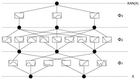
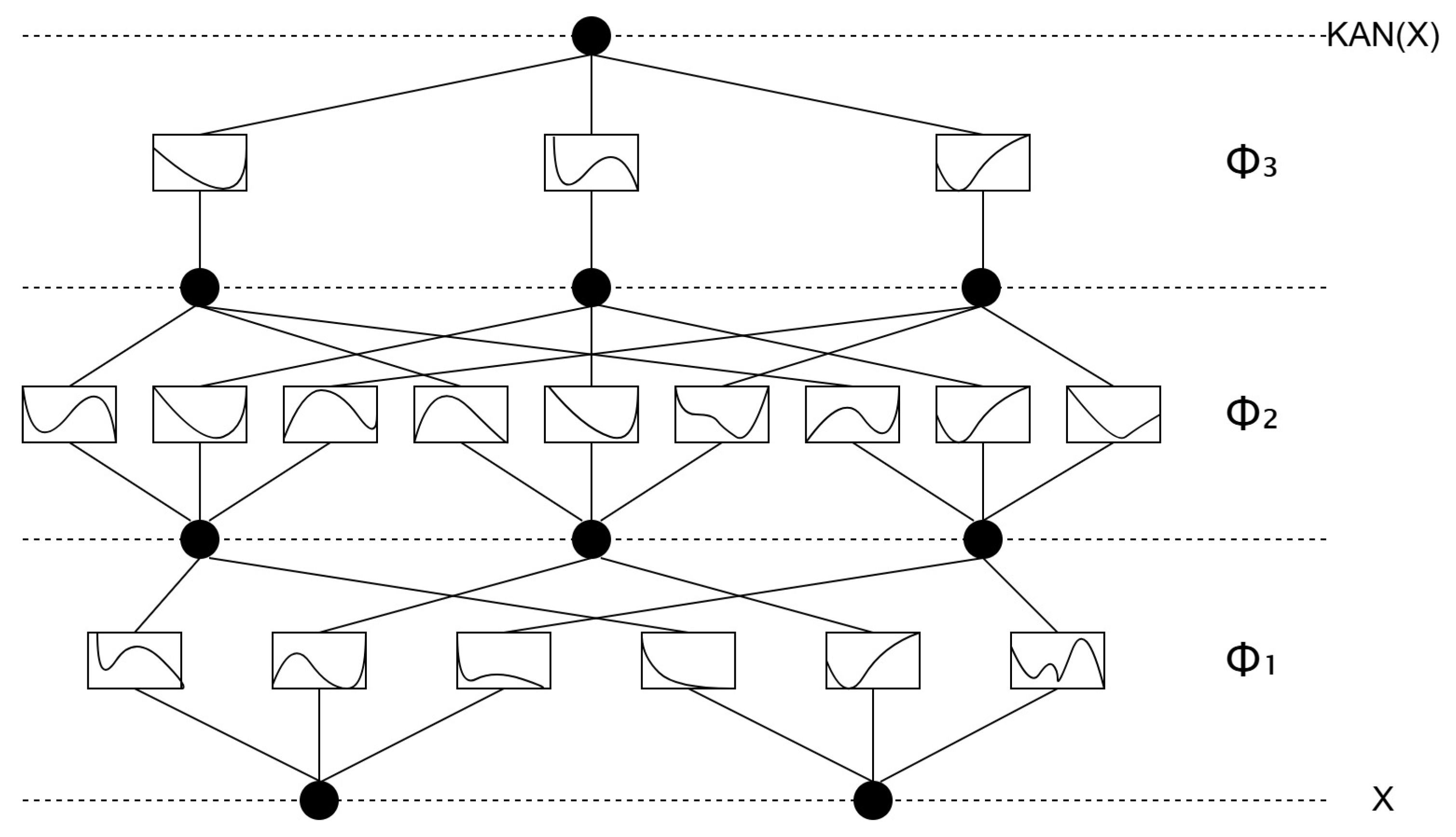
The architectural framework of a KAN is illustrated in Figure 1. By introducing learnable spline-based functions along inter-layer connections, KANs perform adaptive nonlinear transformations on input data, endowing the model with greater flexibility and expressive capacity compared to traditional scalar-weight networks. Moreover, by functionalizing the edges, KANs explicitly reveal variable-wise influence pathways and provide a structurally transparent representation of nonlinear relationships [23,24,25].

Figure 1. Detailed KAN architecture.

2.2. Signature-Weighted Kolmogorov–Arnold Network with Gated Recurrent Unit

2.2.1. Signature-Weighted Kolmogorov–Arnold Network (SigKAN)

Although KANs efficiently approximate complex multivariate mappings via one-dimensional spline transformations, they exhibit limitations in time series tasks. The KAN architecture does not explicitly model temporal dependencies, transition direction, or time-varying interval importance, which can become especially problematic when the target sequence is generated by non-stationary regime switching. In such settings, similar local observations may correspond to different future responses depending on the latent operating state, meaning that a purely static mapping is insufficient to distinguish asymmetric transition paths. Consequently, even though KANs improve nonlinear approximation via spline parameterization, they may still suffer from temporal inconsistency, phase lag, and response smoothing under abrupt dynamic conditions. SigKAN is introduced to remedy these shortcomings while preserving the conventional KAN backbone and incorporating a parallel path signature channel to enhance temporal modeling [26]. This channel extracts path signature features based on rough path theory and employs a gated residual KAN (GRKAN) to generate time-varying channel weights. These weights adaptively fuse the outputs of the KAN branch and the signature channel, yielding a unified representation.

Below, we detail the key modules, namely, the learnable path signature layer and the GRKAN.

Learnable Path Signature Layer

For each input sequence, this layer produces a path signature representation parameterized by learnable weights [27,28]. Consider an N-dimensional path ${\left(X_t\right)}_{t\in [0,T]}$, where $X_t=(X_t^1,\dots ,X_t^N)$. The construction of the path signature begins with the first-order integral

$$\mathcal{S}{\left(X\right)}_{0,t}^n={\int }_0^{t}d{X}_s^n,n\in \{1,\dots ,N\},$$

(5)

which measures the cumulative variation of the path over the interval $[0, t]$.

Next, the second-order iterated integral is constructed as

$$\mathcal{S}{\left(X\right)}_{0,t}^{n,m}={\int }_0^t\mathcal{S}{\left(X\right)}_{0,s}^{n}d{X}_s^m,n,m\in \{1,\dots ,N\},$$

(6)

capturing the interaction relationships among different components. Extension to higher orders yields the general form

$$\mathcal{S}{\left(X\right)}_{0,t}^{i_1,\dots ,i_k}={\int }_0^t\mathcal{S}{\left(X\right)}_{0,s}^{i_1,\dots ,i_{k-1}}d{X}_s^{i_k},i_j\in \{1,\dots ,N\},$$

(7)

forming an infinite sequence of signature terms $\mathcal{S}{\left(X\right)}_{0,T}$. Unlike pointwise temporal descriptors, the path signature is sensitive to the ordered geometry of the trajectory; therefore, it can distinguish sequences with similar marginal amplitudes but different transition directions, accumulation patterns, and cross-channel interactions, which is essential for representing asymmetric production changes. In practice, we truncate the signature at a low order. For the present forecasting task, first-order terms describe cumulative variation and second-order terms encode pairwise interaction and ordering information, which together capture the dominant asymmetric transition patterns. While higher-order terms may provide finer geometric detail, they also rapidly increase feature dimensionality and may yield diminishing returns under limited sample sizes.

Gated Residual KAN (GRKAN)

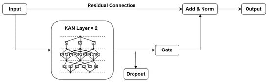
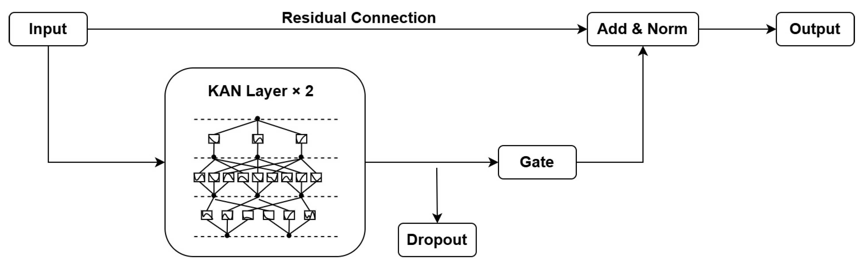
In time series modeling, nonlinear interactions and long-term dependencies are major bottlenecks. Gated residual networks (GRNs) typically offer an efficient mechanism for capturing such relationships by regulating information flow via gating units [29,30]. GRKAN inherits this architecture, following a pipeline of transformation, gating, residual addition, and normalization. Moreover, it introduces a key innovation: it replaces the linear transformation units of standard GRNs with stacked KAN layers, as shown in Figure 2. This integration introduces stronger interpretable nonlinearity while controlling information flow.

Figure 2. Detailed GRKAN architecture.

Formally, the GRKAN formulation is given by

$${\mathrm{GRN}}_{\omega }\left(x\right)=\mathrm{LayerNorm}\left(x+{\mathrm{GLU}}_{\omega }\left({\eta }_1\right)\right),$$

(8)

where the intermediate representations ${\eta }_1$ and ${\eta }_2$ are computed via KAN layers

$$\begin{array}{cc}\hfill {\eta }_1& =\mathrm{KAN}({\varphi }_{{\eta }_1}(·),{\eta }_2),\hfill \end{array}$$

(9)

$$\begin{array}{cc}\hfill {\eta }_2& =\mathrm{KAN}({\varphi }_{{\eta }_2}(·),x).\hfill \end{array}$$

(10)

The gated linear unit (GLU) [31] is defined as

$${\mathrm{GLU}}_{\omega }\left(\gamma \right)=\sigma \left(W_{4,\omega }\gamma +b_{4,\omega }\right)\odot \left(W_{5,\omega }\gamma +b_{5,\omega }\right),$$

(11)

where $\sigma (·)$ denotes the sigmoid activation function. Through this mechanism, the GRKAN adaptively selects important nonlinear contributions while preserving residual connections for stable training. From a regime-switching perspective, this adaptive gating acts as a data-driven reweighting operator, allowing the model to emphasize informative temporal variations and suppress non-critical responses that would otherwise be averaged out under pointwise fitting.

SigKAN Formulation

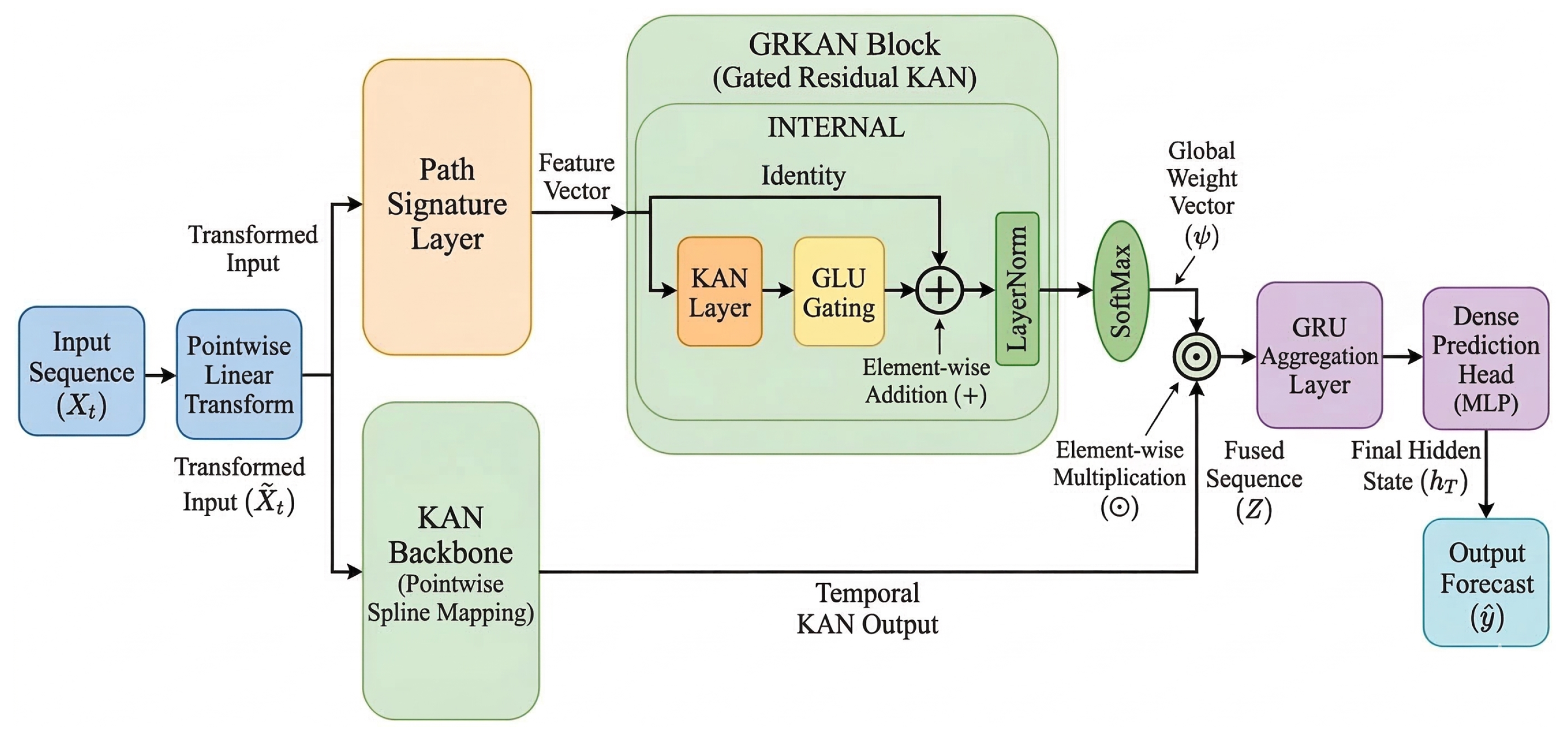
In the SigKAN model, the input path first undergoes a pointwise learnable transformation ${\tilde{X}}_{n,i}=w_n\odot x_{n,i}$. The transformed path $\tilde{X}$ is then fed into the signature layer to compute its truncated signature vector $S\left(\tilde{X}\right)$, encoding high-order geometric characteristics. These features are processed by the GRKAN to produce a hidden representation $h_s$:

$$h_s=\mathrm{GRKAN}\left(S\left(\tilde{X}\right)\right),$$

(12)

then $h_s$ is normalized by a softmax function to obtain a global weight vector $\psi =\mathrm{SoftMax}\left(h_s\right)$. Finally, this vector modulates the output of the main KAN branch to form the weighted temporal sequence $Z={\left\{z_t\right\}}_{t=1}^{\mathrm{seq}}$:

$$z_t=\psi \odot \left(\mathrm{KAN}{\left(\tilde{X}\right)}_t\right),t=1,\dots ,\mathrm{seq}.$$

(13)

Here, the KAN applies transformations point-wise along the temporal dimension, preserving structural integrity; at the same time, $\psi$ imposes a global channel-wise modulation. Beyond independent temporal dependency modeling, SigKAN is designed to capture inter-variable dynamic coupling in multivariate production sequences. This is particularly important for physically related variables such as pressure, choke opening, and oil flow rate, among which interactions are nonlinear and time-varying. First, the path signature representation is computed from the multivariate input trajectory rather than from each variable independently; as a result, the iterated integrals encode not only cumulative variation but also ordered cross-variable interactions, allowing the model to capture coupling patterns such as delayed or asymmetric pressure–production responses. Second, the KAN-based nonlinear transformations operate on the joint representation and learn adaptive local mappings between variables and latent states, which improves the approximation of nonlinear coupled responses. Third, the GRKAN module performs data-driven reweighting over these joint features, emphasizing informative coupling changes under regime transitions. These jointly encoded and reweighted features are then passed to the GRU in the subsequent SigKAN-GRU architecture, where their temporal evolution is further propagated through recurrent hidden states rather than being treated as isolated variable-wise sequences.

2.2.2. SigKAN-GRU Architecture

While SigKAN enhances feature extraction via path signatures and gating, its original design relies on a flatten operation in the output stage. This means that sequential observations are aggregated into a static representation before prediction, without recurrent state propagation across time. In this study, we refer to this limitation as the memory bottleneck: historical information can be encoded, but cannot be explicitly carried forward and updated in a state-dependent manner. As a result, long-range dependencies and regime transitions may be insufficiently preserved, leading to delayed adaptation and smoothed responses. To address this limitation, we propose SigKAN-GRU, which replaces the flatten layer with a GRU to explicitly model temporal dynamics. This replacement is not only architectural but also theoretically motivated: once asymmetric transition features have been extracted and reweighted, they must still be propagated through time in a state-dependent manner. A flatten operation discards this recursive dependency, whereas the GRU preserves regime-sensitive temporal continuity through recurrent state updates.

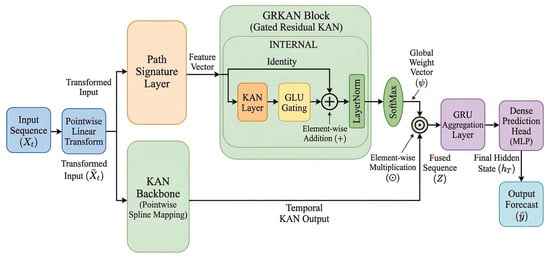
The architecture of SigKAN-GRU is illustrated in Figure 3. Given the weighted fused sequence $Z={\left\{z_t\right\}}_{t=1}^{\mathrm{seq}}$ produced by the SigKAN layer, a GRU is employed to recursively aggregate information along the temporal dimension:

$$h_T=\mathrm{GRU}\left(z_1,\dots ,z_{\mathrm{seq}}\right),h_T\in {\mathbb{R}}^h,$$

(14)

where $h_T$ denotes the hidden state at the final time step. Based on $h_T$, a two-layer fully connected network generates the final prediction:

$$\widehat{\mathbf{y}}=W_2\sigma \left(W_1{h}_T+b_1\right)+b_2,$$

(15)

where $W_1\in {\mathbb{R}}^{100\times h}$, $W_2\in {\mathbb{R}}^{d_{\mathrm{out}}\times 100}$, and $\sigma (·)$ is the activation function.

Figure 3. Detailed architecture of SigKAN-GRU.

In summary, SigKAN-GRU combines the global high-order feature extraction of path signatures with the adaptive gating of GRKAN, then further refines temporal dependency modeling through recurrent aggregation in the GRU. In the final implementation, the KANLinear component adopts a B-spline grid size of 3 and a spline order of 3, which are fixed across all experiments. This design enables the model to capture complex dynamic relationships while preserving a structurally transparent representation of nonlinear response and temporal weighting.

2.2.3. Structural Complexity and Interpretability of SigKAN-GRU

SigKAN-GRU exhibits two structural properties relevant to practical forecasting: controlled complexity and intrinsic interpretability.

For the KAN branch, let d denote the input dimension and m the hidden width. Since each edge is parameterized by a spline with grid size g and order k, the parameter count scales as $\mathcal{O}\left(dm\right(g+k\left)\right)$. In this study, g and k are fixed constants, so the spline complexity grows linearly with the number of input–output connections. For the signature branch, a truncation level q yields feature dimension ${\sum }_{\ell =1}^q{d}^{\ell }$. Under $q=2$, the signature representation is fixed-dimensional and does not grow with the sequence length L. For the recurrent stage, if r is the fused feature width and h is the GRU hidden dimension, the trainable parameter count scales as $\mathcal{O}(rh+h^2+h)$, which is also independent of L. Therefore, under fixed spline order and signature level, SigKAN-GRU maintains controlled parameter growth and reduces the direct sequence-length dependence introduced by flatten-based output heads.

Its interpretability is likewise embedded in the architecture. In the KAN component, each spline function ${\varphi }_{i,j}(·)$ defines an explicit univariate nonlinear mapping, making variable-wise local responses more transparent. In the signature branch, first-order terms describe cumulative variation while second-order terms encode ordered cross-variable interactions, allowing asymmetric transition patterns to be represented explicitly. In addition, the gating vector $\psi =\mathrm{SoftMax}\left(h_s\right)$ provides an explicit weighting over signature-informed channels. Together, these components yield an interpretable representation of nonlinear response, variable interaction, and temporal weighting. From a scalability perspective, this controlled-complexity property is particularly relevant for future multi-well forecasting, since the signature dimension grows with the input dimension under increasing truncation order. Hence, low-order truncation provides a more practical trade-off between geometric expressiveness and computational tractability in larger-scale settings.

3. Experiments

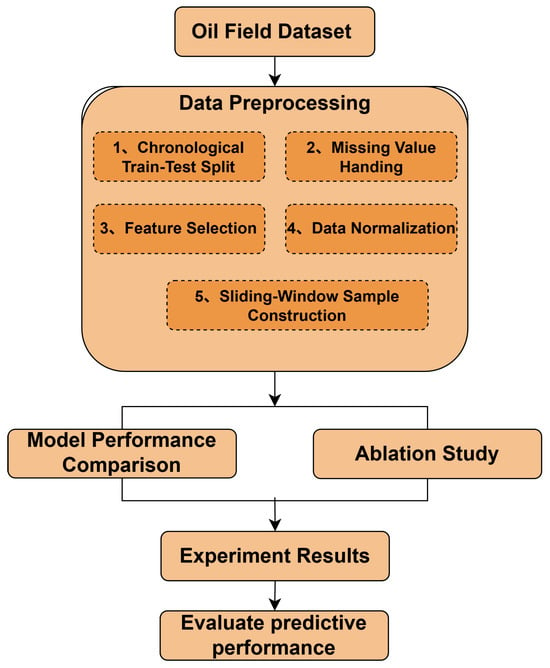
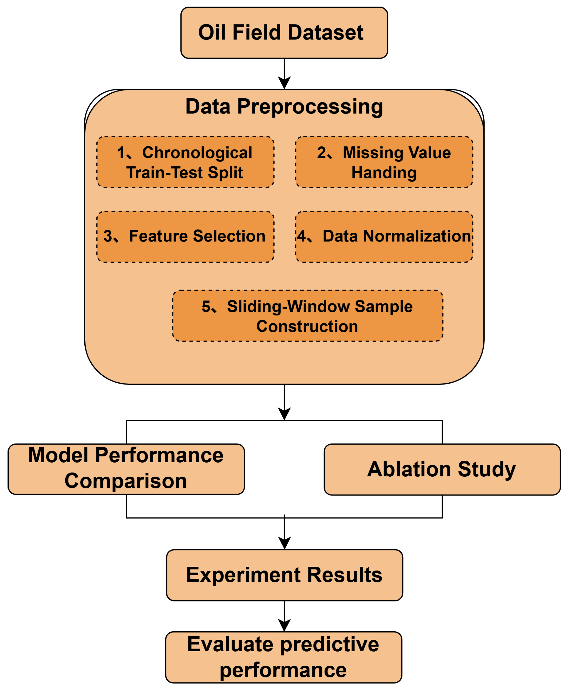
In this section, comparative experiments are conducted using real production data from Well 15/9-F-12 in the Volve Field, Norway and Well No.807 in Western Siberia, Russia in order to evaluate the performance advantages of the proposed SigKAN-GRU model over several representative baselines, including DCA [4], RF [7], LSTM [8], TFT [11], KAN [18], TKAT [19], and TKAN [20]. The comparison set is intended to evaluate the proposed model against representative classical and nonlinear forecasting paradigms under recursive rolling multi-step forecasting. Accordingly, the reported results should be interpreted within the scope of the present benchmark set rather than as a universal comparison against all lag-based forecasting models. Specifically, RF, LSTM, and TFT were retained as widely recognized reference baselines, while KAN, TKAT, and TKAN were selected as recent (2024–2025) temporal KAN-based forecasting models relevant to complex non-stationary dynamics. In addition, internal ablation studies are performed to assess the contribution of each component to the overall performance of SigKAN-GRU. The experimental procedure is as follows: the raw oil production time series are first divided into training and testing subsets in chronological order. All subsequent preprocessing steps, including missing value handling, feature selection, and normalization, are then performed in a leakage-free manner using the training data only, with the learned preprocessing parameters subsequently applied to the test set. The resulting samples are then used for model training and evaluation, and the predictions are analyzed through visualization and multiple quantitative metrics. The experimental workflow is illustrated in Figure 4.

Figure 4. Experimental workflow.

3.1. Dataset Description

The experiment utilizes production data from two wells: Well 15/9-F-12 from the Volve Field, Norway and Well No.807 from Western Siberia, Russia. The Volve Field is located in the North Sea, which initiated production in February 2008 and was decommissioned in September 2016, with a cumulative oil production of about 63 million barrels. In this study, the daily oil production records from the Volve dataset are employed, focusing on data from Well 15/9-F-12 collected between 12 February 2008 and 17 September 2016, consisting of 3056 observations. The two wells considered in this study differ in production setting, measurement availability, and fluctuation characteristics, providing a basis for evaluating the model under heterogeneous data conditions.

Well No.807 is an onshore production well located in Western Siberia, Russia. The dataset covers the daily production history from 2013 to 2021 and, according to the dataset author, was compiled by a chief geologist working in the Siberian oilfields. The data include key parameters such as production rates for oil, liquid, gas, and water, water cut, working hours, dynamic fluid level, and reservoir pressure, making it suitable for analyzing single-well production dynamics as well as for time series forecasting. In this study, the continuous daily records of Well No.807 from 1 January 2013 to 18 January 2021, totaling 2939 observations, are used as the experimental dataset.

3.2. Data Preprocessing

To ensure leakage-free forecasting evaluation in the time series setting, the data processing procedure was organized as follows. First, each dataset was divided into training and testing subsets in chronological order, with the first 80% used for training and the remaining 20% used for testing.

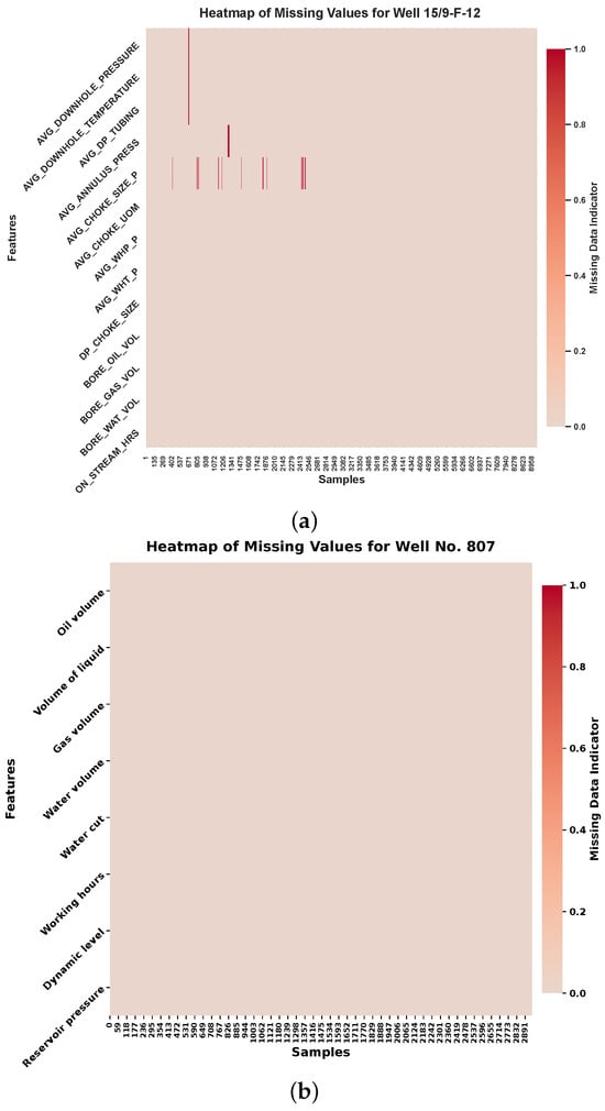
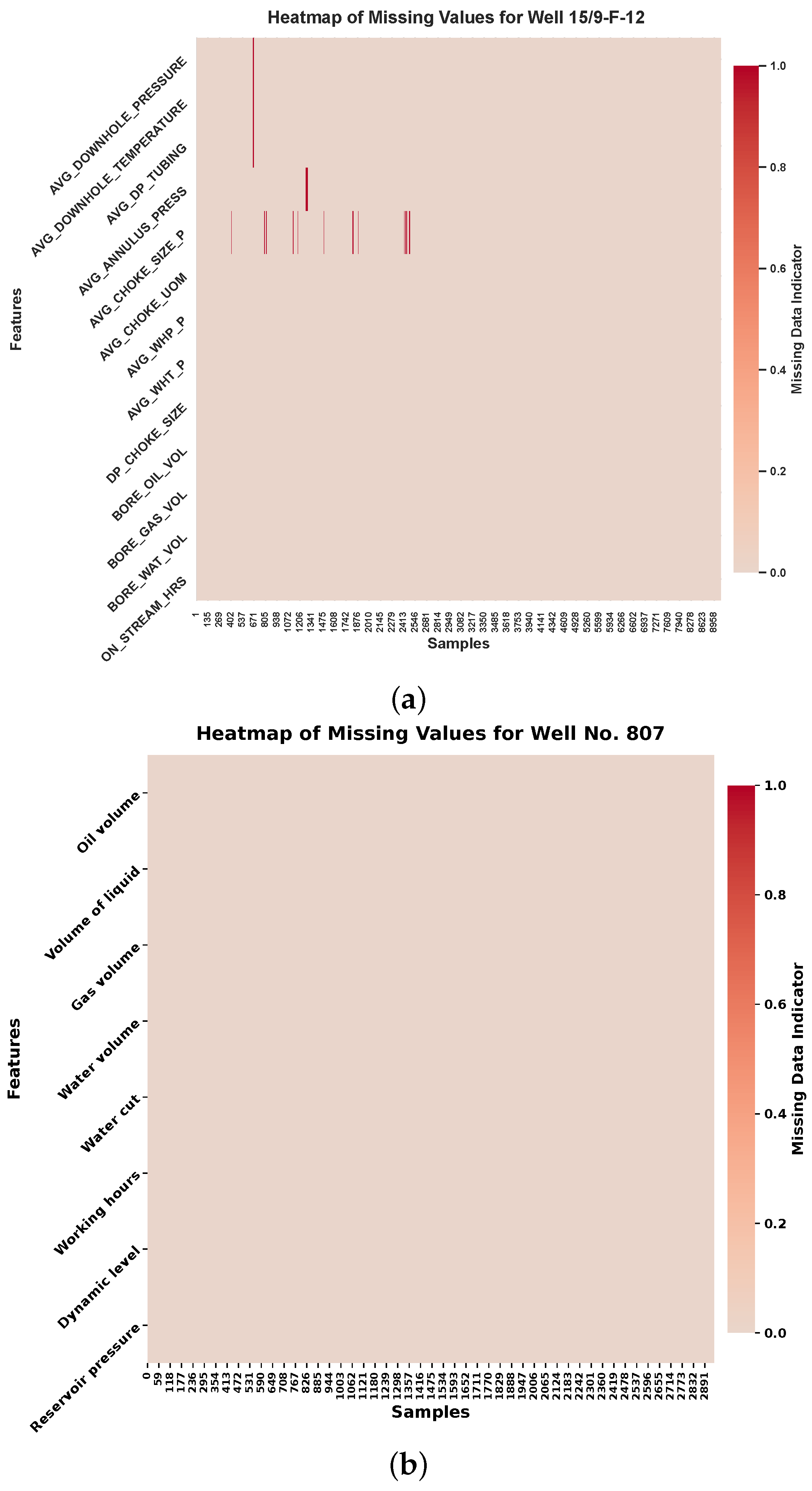
After the split, missing value handling was carried out separately within the training and testing subsets so as to avoid introducing future information across the split boundary. A missing value inspection was first conducted for both wells; the corresponding heatmaps are shown in Figure 5. To preserve temporal order and ensure causality in the forecasting setting, missing values were imputed using a strictly past-only forward-fill strategy. Specifically, each missing entry was replaced by the most recent previously observed value within the same subset, without using any future observations. This operation was performed separately within the training and testing subsets to avoid introducing future information across the train–test split.

Figure 5. Missing value distributions across selected features in two wells: (a) Well 15/9-F-12; (b) Well No.807.

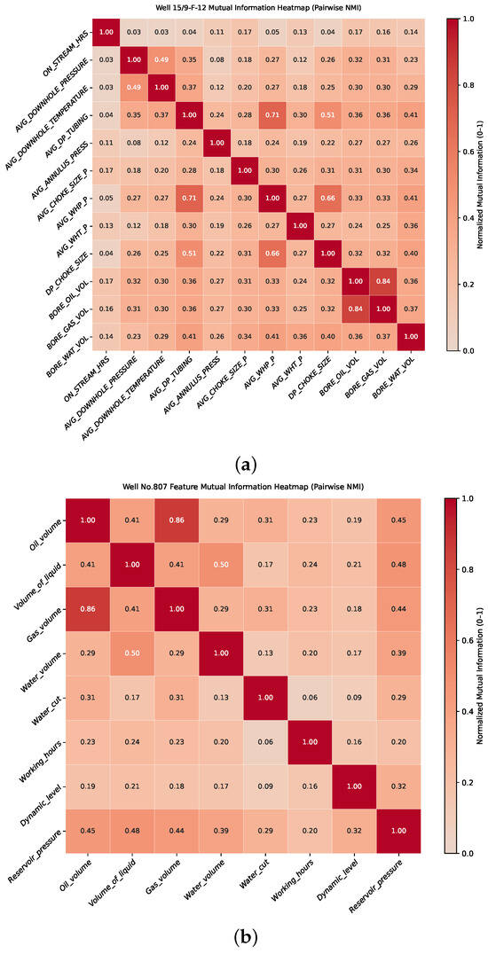
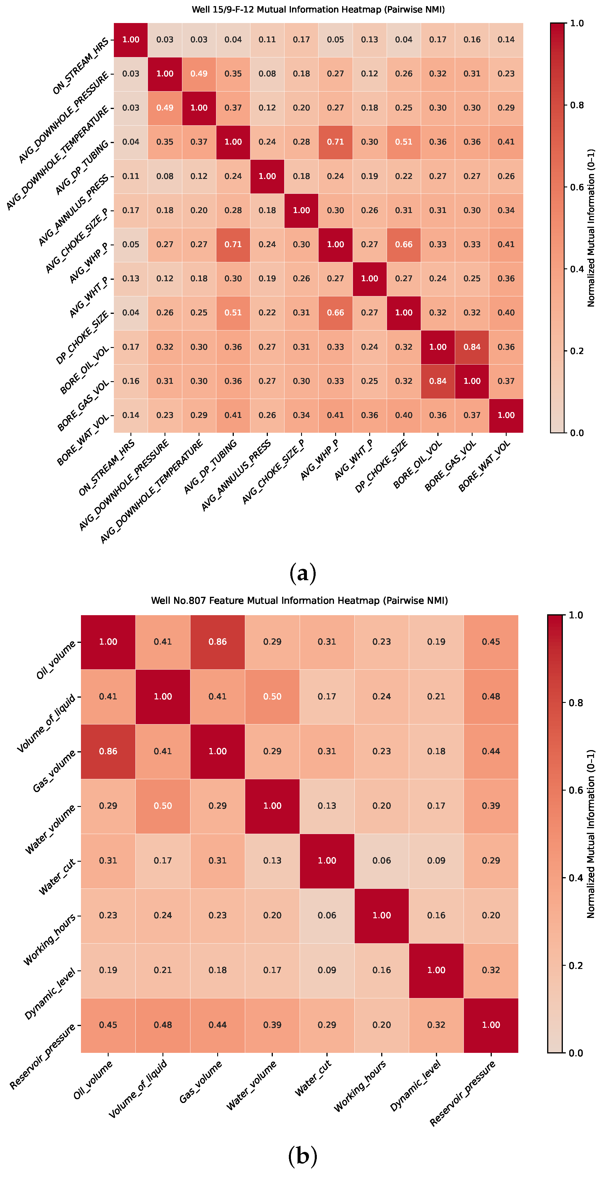
Next, feature selection was performed using the training data only. Given the strong nonlinearity and multivariable coupling in oil production systems, it would be insufficient to rely solely on the Pearson correlation coefficient for assessing feature importance, as it captures only linear relationships. To construct a more informative input set, a nonparametric dependency measure, namely, mutual information (MI), was adopted, since it can capture both linear and nonlinear associations [32]. The MI scores were computed exclusively on the training set, then the selected features were applied to the test set. The resulting MI matrices are shown in Figure 6. It should be emphasized that the MI-based procedure is used only for input selection and redundancy reduction, not for explicit modeling of physical coupling among production variables. The inter-variable dynamic coupling is subsequently learned by the SigKAN-GRU architecture from the joint temporal evolution of the selected variables. From a qualitative petroleum engineering perspective, the selected variables are also physically meaningful for characterizing asymmetric production shifts. For Well 15/9-F-12, AVG_DP_TUBING and AVG_DOWNHOLE_PRESSURE reflect the pressure transfer and inflow conditions between the reservoir and the wellbore, so abrupt changes in these variables may precede uneven production decline or rebound; AVG_WHP_P and DP_CHOKE_SIZE are closely related to surface backpressure and choke-induced flow regulation, which can directly alter production response and amplify asymmetry during operational adjustments. For Well No.807, RESERVOIR_PRESSURE serves as a key indicator of reservoir energy support; therefore, its temporal variation is physically relevant for identifying delayed or asymmetric production responses under depletion and operating fluctuations. For Well 15/9-F-12, the four features with the highest MI scores were selected as the primary input variables, namely, AVG_DP_TUBING (average differential pressure of tubing), AVG_DOWNHOLE_PRESSURE (average downhole pressure), AVG_WHP_P (average wellhead pressure), and DP_CHOKE_SIZE (differential pressure across the choke). In addition, historical oil production was incorporated as a lagged autoregressive feature. Specifically, only past values (e.g., BORE_OIL_VOL at time step $t-1$) were used as inputs to predict production at time t, while the contemporaneous target value was strictly excluded. Therefore, the final input set consists of four MI-selected variables together with one lagged production feature. For Well No.807, because real-time measurements such as wellhead pressure, choke opening, and downhole pressure were not available, it was difficult to fully characterize wellbore dynamics using operational variables alone. According to the MI analysis, RESERVOIR_PRESSURE was selected as the primary explanatory variable. Similarly, historical oil production was included as a lagged autoregressive feature (i.e., OIL_VOLUME at time step $t-1$) to capture temporal dependency while excluding contemporaneous target information.

Figure 6. Mutual information-based dependency analysis of the candidate variables for the two wells: (a) Well 15/9-F-12; (b) Well No.807.

After feature selection, min–max normalization was applied to all continuous variables. The scaling parameters were estimated exclusively from the training data and subsequently applied to the test data to prevent information leakage. In this study, all evaluation metrics were computed in the normalized space after min–max scaling of the target variable. Therefore, the reported error values reflect deviations on the normalized scale rather than in the original physical units. For interpretability, the prediction curves shown in the figures have been transformed back to the original production scale through inverse normalization.

Finally, sliding window samples were constructed. During training, samples were generated in a one-step-ahead supervised manner: for each time step t, an input sequence of length L was formed from historical observations spanning $t-L$ to $t-1$, with the target defined as the value at time t. This formulation was used consistently across all compared models.

During evaluation on the test period, however, forecasting was not performed as an independently conditioned one-step prediction on each test sample; instead, a recursive rolling multi-step forecasting protocol was adopted. Forecasting was initialized from the last available history window at the train–test split point. After the model predicted ${\widehat{y}}_t$, this prediction was fed back into the lagged production position of the next input window; the window was then shifted forward by one step to generate the next forecast, ${\widehat{y}}_{t+1}$. This recursive procedure was repeated until the end of the test horizon. Therefore, ground truth target values from the test period were not used as subsequent lagged inputs during evaluation. In addition, no ground truth future covariates from the test period were injected during rollout. As such, the forecasting process relied only on information available at the forecasting origin together with recursively propagated model outputs. The same protocol was used for all compared models to ensure a fair evaluation.

After the above steps, the resulting training samples were used for model fitting and the recursive rolling forecasts generated on the test set were used for model performance comparison and ablation analysis.

3.3. Evaluation Metrics

To comprehensively evaluate the performance of different models in oil production forecasting, this study establishes a multi-dimensional evaluation framework consisting of three complementary components: overall predictive accuracy, temporal stability, and a supplementary assessment that is both event-sensitive and efficiency-related. Specifically, the overall predictive accuracy is quantified by the mean absolute error (MAE), root mean square error (RMSE), and coefficient of determination ($R^2$). Temporal stability is further characterized by the mean prediction confidence ${\overline{C}}_m$ and stability index $s_m$. In addition, four supplementary indicators, namely, peak-region MAE, shock-delta MAE, trainable parameters, and inference time (ms/sample), are introduced to evaluate model behavior under abrupt transitions, together with computational efficiency.

First, the MAE, RMSE, and $R^2$ are defined as follows:

$$\mathrm{MAE}={\displaystyle \frac{1}{n}}{\displaystyle \sum _{i=1}^n}\left|y_i-{\widehat{y}}_i\right|,$$

(16)

$$\mathrm{RMSE}=\sqrt{{\displaystyle \frac{1}{n}}\sum _{i=1}^n{\left(y_i-{\widehat{y}}_i\right)}^2},$$

(17)

$$R^2=1-{\displaystyle \frac{{\sum }_{i=1}^n{\left(y_i-{\widehat{y}}_i\right)}^2}{{\sum }_{i=1}^n{\left(y_i-\overline{y}\right)}^2}},$$

(18)

where $y_i$ and ${\widehat{y}}_i$ denote the observed and predicted values of the i-th sample, respectively, $\overline{y}$ denotes the mean of the observed values, and n is the total number of samples. Among these metrics, MAE measures the average magnitude of prediction errors, RMSE places greater emphasis on large deviations, and $R^2$ reflects the overall explanatory capability of the model.

Second, to further characterize temporal consistency and robustness, the instantaneous confidence of model m at time step i is defined as

$$C_{mi}=1-{\displaystyle \frac{{\left({\widehat{y}}_{mi}-y_i\right)}^2}{{\sum }_{k=1}^M{\left({\widehat{y}}_{ki}-y_i\right)}^2}},$$

(19)

where ${\widehat{y}}_{mi}$ and $y_i$ denote the predicted and true values at time step i, respectively, and M is the total number of compared models. Based on $C_{mi}$, the mean prediction confidence of model m is computed as

$${\overline{C}}_m={\displaystyle \frac{1}{N}}{\displaystyle \sum _{i=1}^N}{C}_{mi},$$

(20)

where N is the number of aligned test time steps. A larger ${\overline{C}}_m$ indicates that the model performs better on average relative to the other models within the same comparison group. The stability index $s_m$, which quantifies the temporal fluctuation of confidence, is defined as

$$s_m=\sqrt{{\displaystyle \frac{1}{N-1}}\sum _{i=1}^N{\left(C_{mi}-{\overline{C}}_m\right)}^2.}$$

(21)

A smaller $s_m$ indicates more stable and robust predictive performance over time. In practice, the confidence-based metrics are computed separately within each experimental group. For both the main comparison experiments and the ablation study, the predictions of all models are first aligned on the common test timestamps shared within the corresponding group. The denominator in Equation (19) is then constructed from the squared prediction errors of all models at each aligned time step. Accordingly, the reported values of ${\overline{C}}_m$ and $s_m$ should be interpreted as group-specific relative measures rather than as absolute performance indicators.

Third, to supplement the above global and stability-oriented metrics, four additional indicators are reported: peak-region MAE, shock-delta MAE, trainable parameters, and inference time (ms/sample). The peak-region MAE evaluates the absolute prediction error in the vicinity of local extrema, whereas the shock-delta MAE measures the error in first-order production changes during abrupt transition intervals. Trainable parameters quantifies model complexity, while inference time reflects computational efficiency in terms of the average per-sample inference latency measured on the test set after model fitting. Let $\mathcal{P}$ denote the index set of samples located within a fixed window around local extrema of the ground-truth production sequence, and let $\mathcal{S}$ denote the index set of abrupt transition intervals identified from the first-order difference series of the ground-truth sequence. The two event-sensitive metrics are defined as follows:

$${\mathrm{MAE}}_{\mathrm{peak}}={\displaystyle \frac{1}{\left|\mathcal{P}\right|}}\sum _{t\in \mathcal{P}}\left|y_t-{\widehat{y}}_t\right|,$$

(22)

$${\mathrm{MAE}}_{\Delta \mathrm{shock}}={\displaystyle \frac{1}{\left|\mathcal{S}\right|}}\sum _{t\in \mathcal{S}}\left|\left(y_t-y_{t-1}\right)-\left({\widehat{y}}_t-{\widehat{y}}_{t-1}\right)\right|.$$

(23)

In summary, MAE, RMSE, and $R^2$ are used to evaluate overall predictive accuracy, whereas ${\overline{C}}_m$ and $s_m$ characterize temporal stability and robustness; ${\mathrm{MAE}}_{\mathrm{peak}}$ and ${\mathrm{MAE}}_{\Delta \mathrm{shock}}$ further assess event-sensitive performance under abrupt production transitions, while trainable parameters and inference time quantify model complexity and computational efficiency. Taken together, these metrics provide a more comprehensive evaluation of model performance in oil production forecasting.

3.4. Parameter Optimization

Time series forecasting models are often sensitive to hyperparameter choices, and using default settings may lead to unstable training and suboptimal predictive performance; therefore, Bayesian optimization was employed for the trainable learning-based models in this study [33]. Bayesian optimization models the relationship between hyperparameters and validation performance through a surrogate-based search strategy, improving search efficiency by balancing exploration of uncertain regions and exploiting promising configurations.

The optimization objective was the validation MAE under a time series-aware validation split. MAE was adopted as the primary criterion because of its robustness to outliers, whereas RMSE and $R^2$ were used only for comprehensive post hoc evaluation.

To improve model-level reproducibility, the revised manuscript now distinguishes explicitly between model-specific hyperparameter search spaces and final selected configurations. Table 2 summarizes the model-specific hyperparameter search spaces, whereas Table 3 reports the final selected configurations adopted in the experiments. Unless otherwise stated, parameters not listed in Table 2 were kept fixed throughout the optimization process.

Table 2. Model-specific hyperparameter search spaces.

Model	Tuned Hyperparameters	Search Space
DCA	Decline form	{exponential, harmonic, hyperbolic}
	Fitted parameters	Arps parameters estimated by nonlinear least squares
RF	Number of trees	{100, 200, 300, 500}
	Min samples (internal)	{2, 4, 8}
	Min samples (leaf)	{1, 2, 4}
	Feature subsampling	{0.2, 0.4, 0.6}
LSTM	Hidden units	[16, 128]
	FC layer width	{8, 16, 32, 64}
	Dropout	{0.0, 0.1, 0.2, 0.3}
	Learning rate	[${10}^{-4},{10}^{-2}$]
	Batch size	{16, 32, 64}
TFT	Representation dimension	{32, 64, 96, 128}
	Attention heads	{1, 2, 3, 4}
	Feed-forward width	{64, 128, 256}
	Learning rate	[${10}^{-4},{10}^{-2}$]
	Batch size	{16, 32, 64}
KAN	Spline-linear mapping width	[64, 256]
	Learning rate	[${10}^{-4},{10}^{-2}$]
	Batch size	{16, 32, 64}
TKAN	Units	[32, 128]
	Sub-KAN output dimension	[8, 32]
	Number of modules	{1, 2, 3}
	Learning rate	[${10}^{-4},{10}^{-2}$]
	Batch size	{16, 32, 64}
TKAT	Model dimension ($d_{\mathrm{model}}$)	{48, 72, 96, 120}
	Number of blocks	{1, 2, 3, 4}
	Attention heads	{1, 2, 3, 4}
	Learning rate	[${10}^{-4},{10}^{-2}$]
	Batch size	{16, 32, 64}
SigKAN-GRU	Signature level	{1, 2, 3}
	KANLinear width	[64, 256]
	GRU hidden dimension	[32, 128]
	Dense layer width	{32, 64, 128}
	Learning rate	[${10}^{-4},{10}^{-2}$]
	Batch size	{16, 32, 64}

Note: For SigKAN-GRU, the spline grid size $g=3$ and spline order $k=3$ were fixed across all experiments. The input sequence length was fixed to $L=14$ for all models.

Table 3. Final model configurations and selected hyperparameter values.

Model	Structural Parameters & Configuration	Learning Rate	Batch Size
DCA	Arps decline model; candidate forms: exponential, harmonic, and hyperbolic; exponential form selected on the training segment;	-	-
RF	Trees: 200; Min samples (internal): 4; Min samples (leaf): 2; Feature subsampling: 0.2	-	-
LSTM	Hidden units: 32; FC layer: 16 neurons; Dropout: 0.1;	0.001	32
TFT	Representation dim: 64; Attention heads: 3; Feed-forward width: 128	0.001	16
KAN	Spline-linear mapping width: 128	0.002	16
TKAN	Units: 80; Sub-KAN output dim: 20; Grid size: 3; Modules: 2 sequential	0.0015	32
TKAT	Model dim ($d_{\mathrm{model}}$): 72; Blocks: 3; Attention heads: 2	0.0016	64
SigKAN-GRU	SigLayer(2) + GRKAN + KANLinear(144; $g=3,k=3$) → GRU(56) → Dense(64)	0.00259	32

Note: The input sequence length is uniformly set to $L=14$ for all models. This table reports the selected hyperparameter settings for each model class. Because the final input dimensionality differs across wells after feature selection, the instantiated trainable parameter counts and inference times reported in later tables may vary across wells even under the same hyperparameter configuration.

For the proposed SigKAN-GRU model, Bayesian optimization was used to tune the signature level, KANLinear width, GRU hidden dimension, dense layer width, learning rate, and batch size; in contrast, the spline grid size $g=3$ and spline order $k=3$ were fixed across all experiments. The optimal signature level was selected as 2 from the candidate set $\{1,2,3\}$, suggesting that second-order path geometry already provides sufficient discriminatory information for the asymmetric production dynamics considered in this study. This choice reflects a practical trade-off between representational richness and computational cost. In the present task, first-order signature terms describe cumulative variation, while second-order terms encode pairwise interaction and ordering information; together, they are sufficient to capture the dominant asymmetric transition patterns. By contrast, higher-order truncation levels provide finer geometric detail but rapidly increase the signature feature dimension as ${\sum }_{\ell =1}^q{d}^{\ell }$, which in turn raises memory and optimization costs. Therefore, selecting $q=2$ offers a favorable balance between expressive power and controlled complexity. This consideration becomes even more important when scaling to multi-well settings, where the effective input dimension may increase due to the inclusion of additional wells and cross-well interactions, making higher-order signatures progressively more expensive.

For the DCA baseline, no Bayesian hyperparameter search was performed; instead, the decline form was selected from the candidate set {exponential, harmonic, hyperbolic}, and the corresponding Arps parameters were fitted on the training segment only. The exponential form was finally retained. For the remaining baselines, the final configurations obtained from the model-specific search procedure are listed in Table 3.

3.5. Results and Discussion

3.5.1. Model Performance Comparison

Visual Comparison

To verify the superiority of the proposed SigKAN-GRU model, a comparative study was carried out against seven representative baselines, namely, DCA, RF, LSTM, TFT, KAN, TKAN, and TKAT, in the oil production forecasting tasks of both Well 15/9-F-12 and Well No.807. This covers widely used reference models as well as recent temporal KAN-based forecasting architectures.

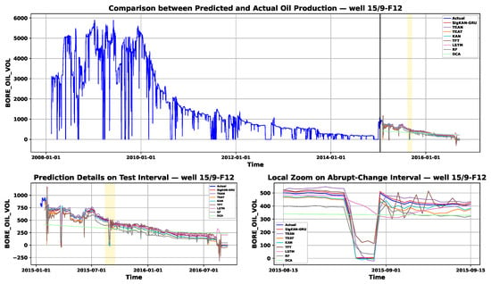
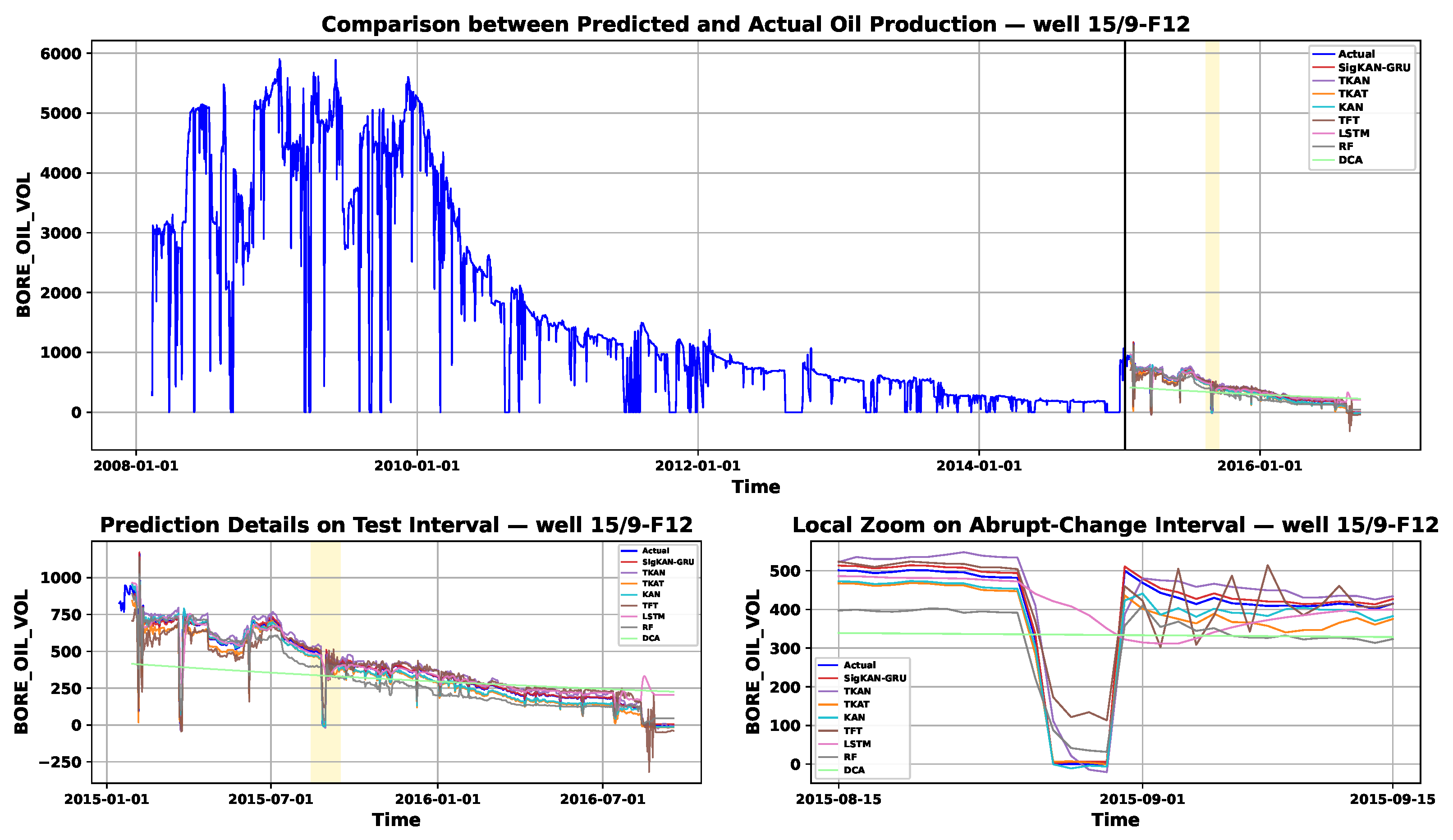
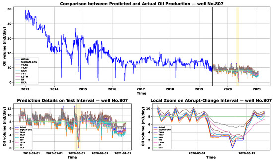
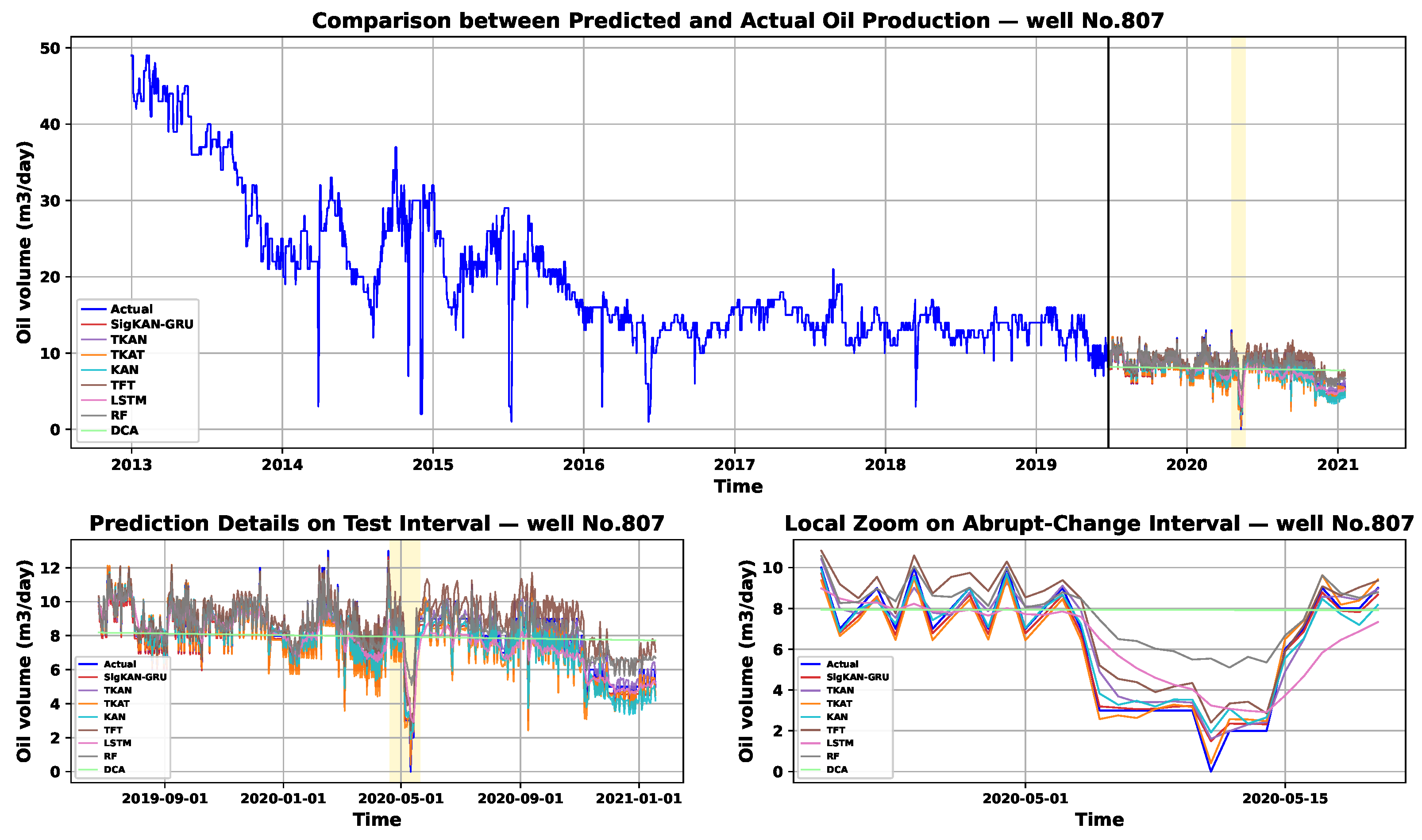
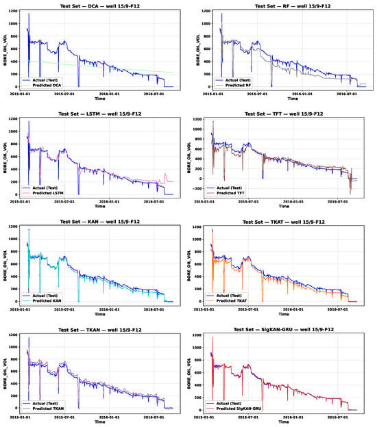
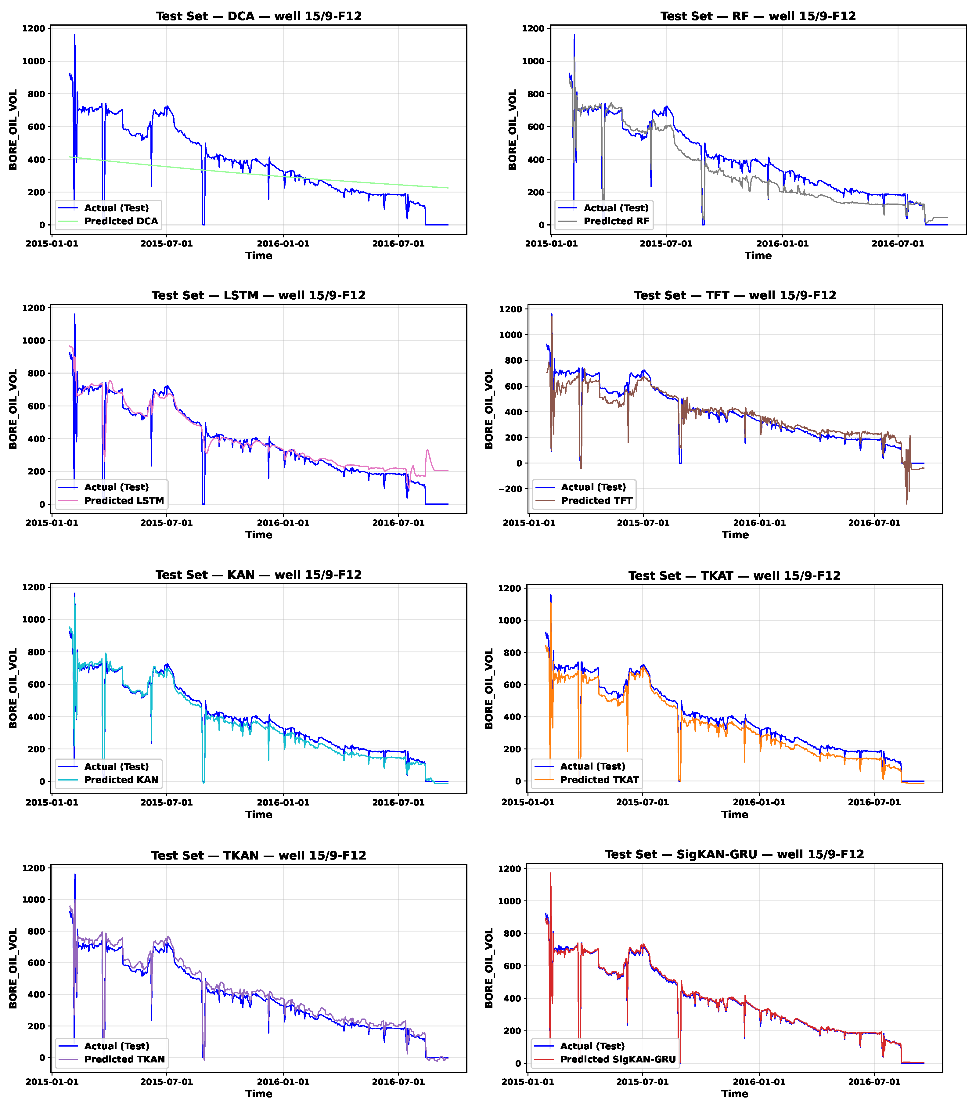
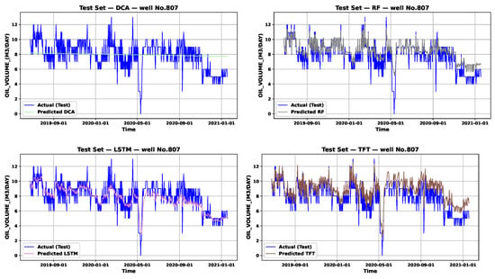
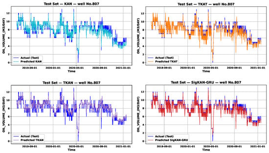
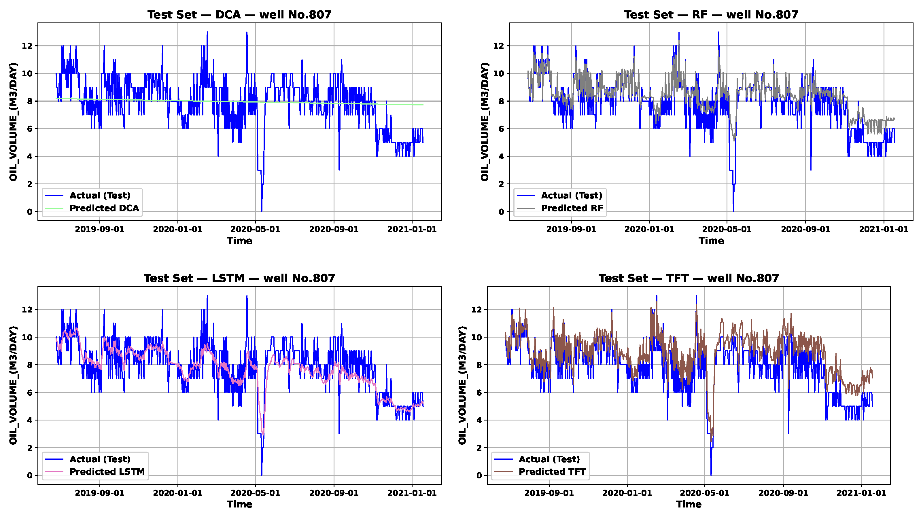
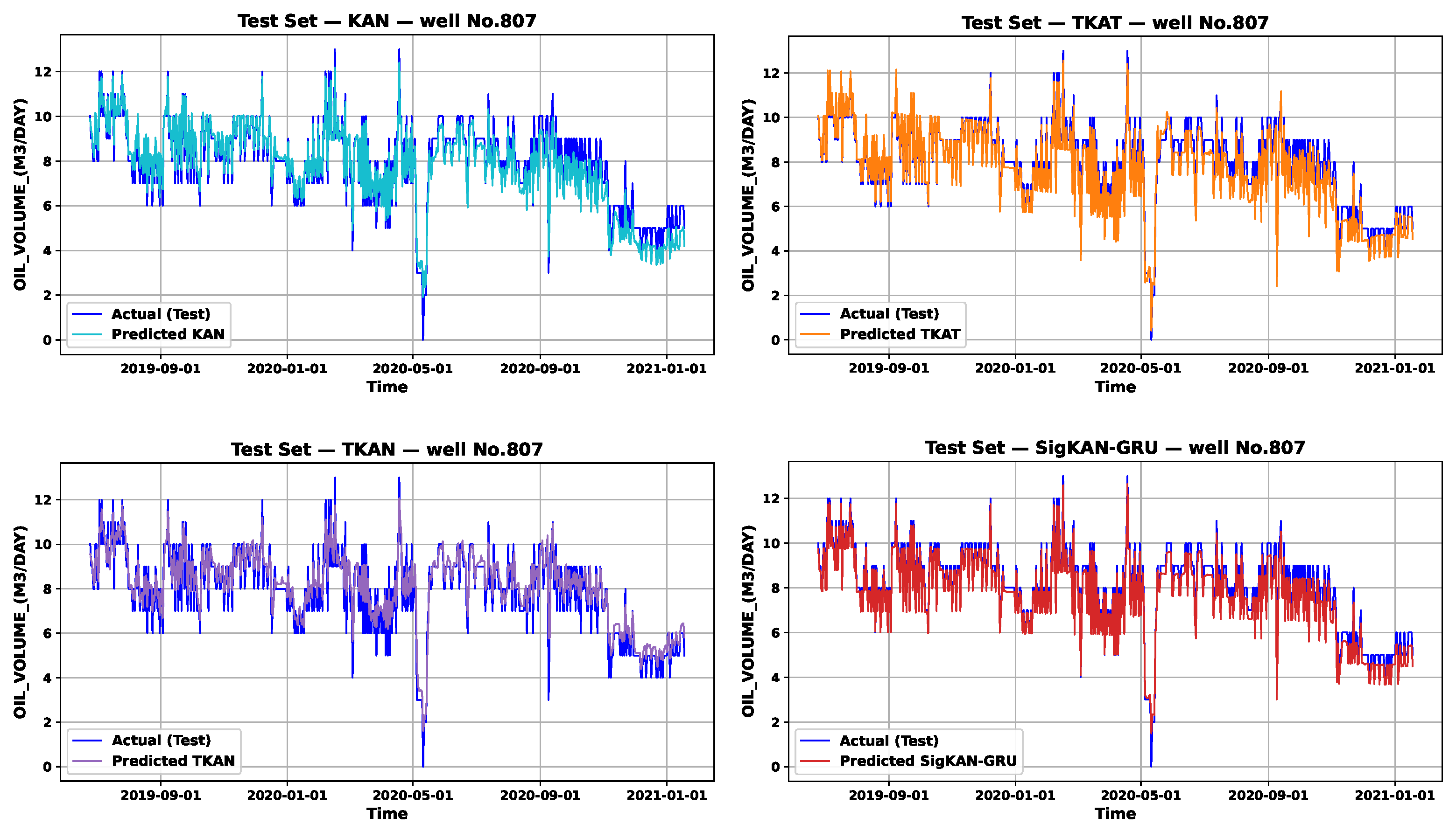
We first conduct a qualitative evaluation of the predicted trajectories to visually assess the fitting capability of the models. Figure 7 and Figure 8 illustrate the overall predictive accuracy and temporal alignment of the eight compared models on Well 15/9-F-12 and Well No.807, respectively. Detailed well-by-well visual comparisons for each individual model are further provided in Figure 9 and Figure 10. Compared to other models, the predicted curves of SigKAN-GRU align closely with the measured data in both phase and amplitude, accurately capturing rapid production fluctuations and trend transitions. SigKAN-GRU effectively eliminates the time lag commonly observed in LSTM and TKAN and mitigates the over-smoothing issue in TFT. In the highly fluctuating environment of Well No.807, SigKAN-GRU maintains smaller residual bands and higher stability, avoiding the oscillatory errors exhibited by RF and TKAT under high-frequency noise. It should be noted that these sharp declines are captured under the recursive rolling multi-step forecasting protocol described in Section 3.2 rather than under a conditional one-step evaluation. Once forecasting enters the test period, neither ground-truth test targets nor future test-period covariates are fed back as subsequent inputs. Therefore, the close alignment around abrupt production drops should be interpreted as the result of forecasting from historical precursors and recursively propagated predictions rather than as a consequence of conditional access to $y_{t-1}$ from the test period.

Figure 7. Overall comparison on Well 15/9-F-12. The main plot illustrates the global production trajectory over the entire history, while the detailed view focuses on the test interval performance. The zoomed-in inset (bottom right), indexed by the light yellow bar in the main plot, highlights the specific abrupt transition interval to demonstrate the model’s superior phase alignment and rapid tracking capability compared to other baselines.

Figure 8. Overall comparison on Well No.807. The main plot illustrates the global production trajectory over the entire history, while the detailed view focuses on the test interval performance. The zoomed-in inset (bottom right), indexed by the light yellow bar in the main plot, highlights the specific abrupt transition interval to demonstrate the model’s superior phase alignment and rapid tracking capability compared to other baselines.

Figure 9. Test set predictions for Well 15/9-F-12.

Figure 10. Test set predictions for Well No.807.

Overall Quantitative Performance

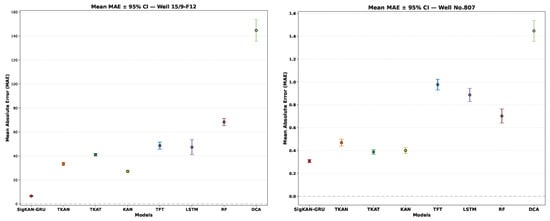
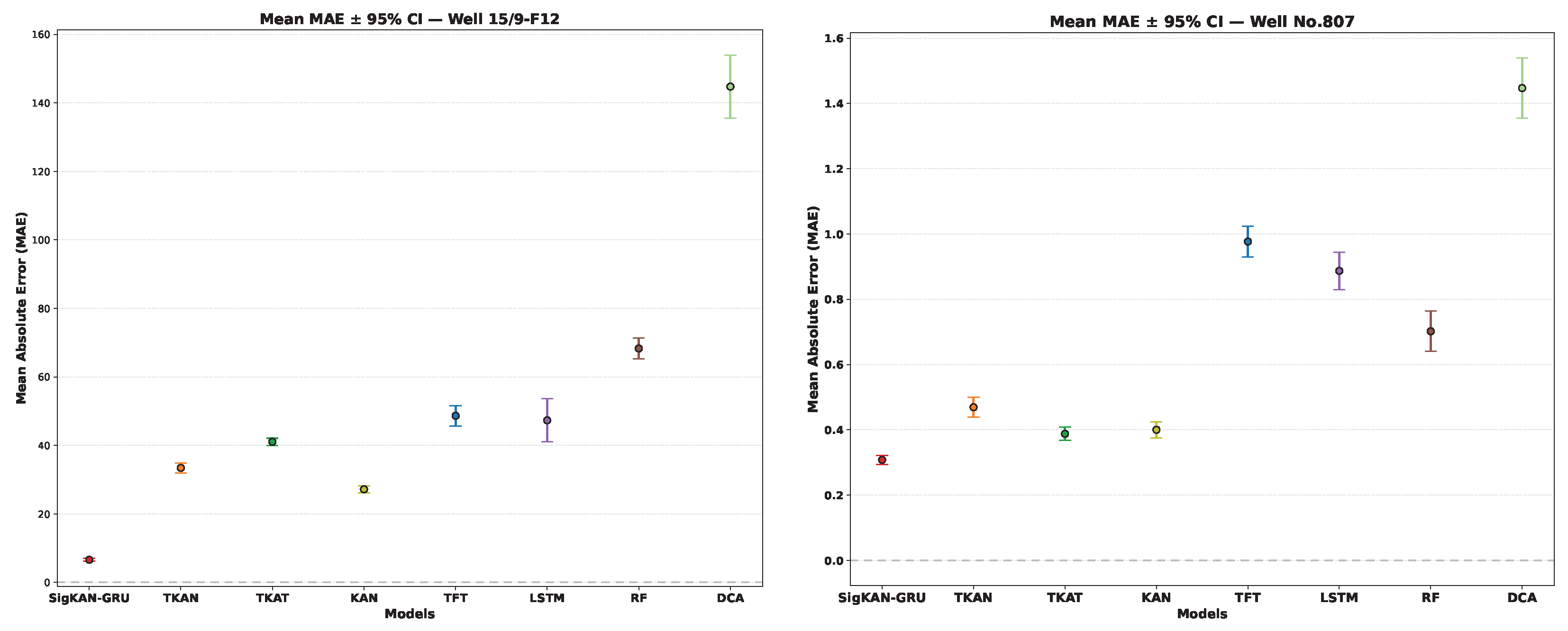
While trajectory alignment offers visual confirmation, a more rigorous evaluation requires quantifying the distribution of prediction errors on the test set. Figure 11 reports the mean MAE together with its 95% confidence interval for eight models in total, including SigKAN-GRU and seven baselines, on the two wells.

Figure 11. Mean MAE with 95% confidence intervals estimated from the distribution of absolute prediction errors over the aligned test samples. Different colors correspond to the respective models labeled on the axis. Within each boxplot, the central line denotes the median error, and the colored dots represent outlier prediction errors.

For each model, the absolute errors $e_i=|y_i-{\widehat{y}}_i|$ are computed over all aligned test samples, and the mean MAE together with its 95% confidence interval is estimated from their sample distribution. The 95% confidence interval is given by

$$\overline{e}\pm t_{0.975,n-1}{\displaystyle \frac{s_e}{\sqrt{n}}},$$

(24)

where $\overline{e}$ is the mean absolute error, $s_e$ is the sample standard deviation of the absolute errors, and n is the number of aligned test samples. Therefore, the interval reflects the uncertainty of the average prediction error across the test samples rather than the variability across repeated training runs.

SigKAN-GRU exhibits both the lowest average MAE and the narrowest confidence intervals on both wells, indicating that its prediction errors are not only smaller on average but also more concentrated across the test samples. To further quantify the above observations, Table 4 summarizes the quantitative performance of all compared models across the two wells. The table reports the major evaluation indicators ($R^2$, MAE, RMSE, ${\overline{C}}_m$, and $s_m$) for a concise numerical comparison. For Well 15/9-F-12, SigKAN-GRU attains an $R^2$ of 0.9986, suggesting an almost perfect fit to the actual production data. Its MAE and RMSE decrease by approximately 70–80%, reflecting a substantial reduction in both absolute and squared errors at global and local levels. For Well No.807, the $R^2$ increases to 0.9657, while MAE and RMSE decrease by about 20–25%, demonstrating high prediction precision and stability even under complex operational and highly fluctuating conditions. Overall, SigKAN-GRU achieves consistently higher $R^2$ values and lower MAE/RMSE across the two wells, confirming its strong ability to capture nonlinear dynamic features and temporal dependencies. Beyond standard accuracy, the temporal reliability of the forecasts is further corroborated by the confidence-based metrics. As shown in the last two columns of Table 4, SigKAN-GRU achieves ${\overline{C}}_m=0.9984$ and $s_m=0.0029$ on Well 15/9-F-12, corresponding to a gain of $+0.0400$ in ${\overline{C}}_m$ and a 92.6% reduction in $s_m$ compared with the best baseline. For Well No.807, ${\overline{C}}_m$ increases to 0.9756 and $s_m$ decreases to 0.0210, corresponding to a gain of $+0.0153$ in ${\overline{C}}_m$ and a 60.1% reduction in $s_m$ relative to the best baseline. These results indicate that SigKAN-GRU remains optimal or near-optimal at the majority of time steps and that its performance advantage fluctuates only slightly over time, highlighting its superior temporal stability.

Table 4. Comprehensive comparison of models on Well 15/9-F-12 and Well No.807.

Well	Model	${\mathit{R}}^2$	MAE	RMSE	${\overline{\mathit{C}}}_{\mathit{m}}$	${\mathit{s}}_{\mathit{m}}$
Well 15/9-F-12	DCA	0.2985	0.0245	0.0313	0.5651	0.2965
	RF	0.8740	0.0116	0.0133	0.7486	0.2310
	LSTM	0.8262	0.0080	0.0156	0.9225	0.1403
	TFT	0.9228	0.0082	0.0104	0.9242	0.0695
	KAN	0.9812	0.0046	0.0051	0.9566	0.0422
	TKAT	0.9618	0.0070	0.0073	0.9262	0.0552
	TKAN	0.9702	0.0057	0.0064	0.9584	0.0394
	SigKAN-GRU	0.9986	0.0011	0.0014	0.9984	0.0029
Well No.807	DCA	0.0590	0.0301	0.0382	0.6493	0.2624
	RF	0.7051	0.0146	0.0214	0.9016	0.1078
	LSTM	0.6428	0.0185	0.02336	0.8276	0.1662
	TFT	0.6397	0.0203	0.0237	0.7837	0.1776
	KAN	0.9297	0.0083	0.0105	0.9603	0.0526
	TKAT	0.9412	0.0081	0.0096	0.9559	0.0531
	TKAN	0.8999	0.0098	0.0125	0.9462	0.0646
	SigKAN-GRU	0.9657	0.0064	0.0073	0.9756	0.0210

Note: MAE and RMSE are computed in the normalized space after min–max scaling of the target variable.

The consistency between the quantitative metrics and the visual comparisons indicates that SigKAN-GRU delivers the strongest overall performance within the current baseline set, combining higher numerical accuracy with more stable predictive behavior under the recursive rolling forecasting protocol.

Event-Sensitive and Efficiency Evaluation

While Table 4 summarizes the overall predictive accuracy and temporal stability, practical oil production forecasting also requires reliable model discrimination under abrupt transition regimes together with an explicit comparison of model complexity and inference efficiency. Therefore, Table 5 further reports two event-sensitive metrics, peak-region MAE and shock-$\Delta$ MAE, along with two efficiency-related metrics, trainable parameters and inference time, for all compared models on both wells.

Table 5. Event-sensitive and efficiency comparison of models on Well 15/9-F-12 and Well No.807.

Well	Model	Peak MAE	Shock-$\Delta$ MAE	Params	Inf.Time (ms/Sample)
Well 15/9-F-12	DCA	182.8203	155.8451	2	0.00004
	RF	75.2731	73.8333	N/A	0.0784
	LSTM	116.4040	141.9159	5409	1.2907
	TFT	58.2687	28.1386	28,182	1.4816
	KAN	33.6902	19.3931	250,497	1.0259
	TKAT	43.8169	10.4674	334,541	5.0445
	TKAN	141.4125	49.0962	78,166	13.6335
	SigKAN-GRU	9.1433	5.2759	264,608	2.2239
Well No.807	DCA	2.0312	3.4928	2	0.00005
	RF	1.2546	2.0406	N/A	0.0532
	LSTM	0.8464	1.3466	6113	1.3240
	TFT	0.3273	0.3086	150,401	2.3747
	KAN	1.0108	0.3701	139,777	1.0001
	TKAT	0.1349	0.0343	491,229	4.4633
	TKAN	0.7522	1.2033	77,431	14.0191
	SigKAN-GRU	0.2795	0.1239	307,416	2.3391

Note: Inf.Time (ms/sample) denotes the average per-sample inference latency measured on the test set after model fitting, rather than the training or fitting time. For RF, trainable parameter count is not defined in the same way as neural network models. For DCA, the reported inference time corresponds to the evaluation time of the fitted decline equation over the test horizon.

As shown in Table 5, SigKAN-GRU demonstrates strong event-sensitive predictive capability while achieving a favorable trade-off between predictive performance and computational cost. On Well 15/9-F-12, it achieves the lowest peak-region MAE and shock-$\Delta$ MAE by a clear margin, indicating superior fidelity in both local extrema and abrupt production transitions. On the more volatile Well No.807, although TKAT attains the smallest event-sensitive errors, SigKAN-GRU remains among the top-performing models while requiring substantially fewer parameters and lower inference latency than TKAT. These results suggest that the proposed model does not pursue minimum complexity in an absolute sense; instead, it offers a more favorable balance between shock robustness, predictive accuracy, and computational efficiency. The motivation for the added architectural complexity is not merely to improve the average error metrics but to better capture asymmetric transition dynamics under recursive rollout. This is particularly reflected in the event-sensitive indicators, where the proposed model shows improved fidelity around local extrema and abrupt production changes. From a deployment perspective, although SigKAN-GRU has a substantially larger parameter count than a standard LSTM, its inference latency in Table 5 remains at the millisecond-per-sample level. This suggests that the model is feasible for deployment on edge-side industrial hardware with moderate computing resources, such as field gateways or on-site industrial PCs, where inference rather than training is performed locally. However, for highly resource-constrained embedded devices, additional model compression techniques such as pruning, quantization, or distillation would likely be necessary.

Gaussian Noise Sensitivity Analysis

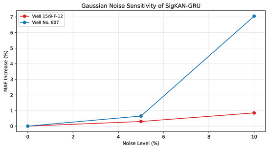
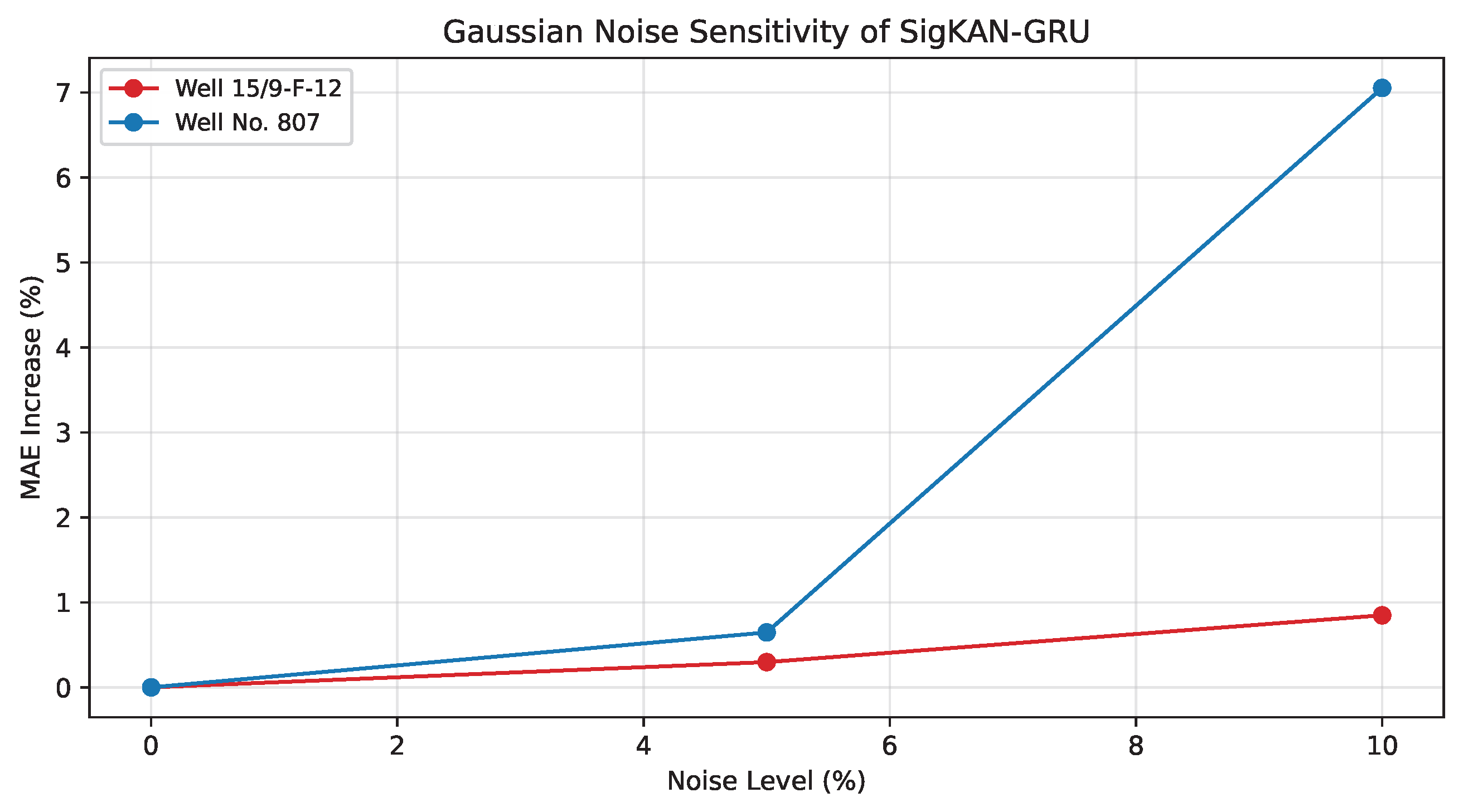
To further examine robustness against sensor disturbances, we conducted a supplementary Gaussian noise sensitivity analysis at the inference stage. Specifically, Gaussian perturbations with noise levels of 5% and 10% were injected into the test inputs of SigKAN-GRU while keeping all trained model parameters unchanged. Figure 12 shows that the relative MAE increases with the noise level on both wells. For Well 15/9-F-12, the increase remains below 1% even at the 10% noise level, indicating strong robustness to moderate perturbations. For Well No.807 the degradation is more pronounced, likely due to its more limited input feature set and higher intrinsic volatility, but the model still maintains stable prediction behavior under moderate synthetic noise.

Figure 12. Gaussian noise sensitivity analysis of SigKAN-GRU on Well 15/9-F-12 and Well No.807. The figure reports the relative MAE increase under 5% and 10% Gaussian perturbations injected into the test inputs.

3.5.2. Ablation Study

To isolate and quantify the marginal contribution of each architectural component to the overall predictive performance, we conducted a systematic ablation study of the SigKAN-GRU framework. To provide a direct comparison with the proposed SigKAN-GRU, the standalone SigKAN model (without the GRU-based temporal aggregation) is included as a baseline. While maintaining identical data partitioning, training protocols, and evaluation metrics, we progressively excluded or substituted key modules of the model. The resulting variants were evaluated using $R^2$, MAE, and RMSE as well as the mean (${\overline{C}}_m$) and standard deviation ($s_m$) of the relative confidence metric to assess both accuracy and stability.

The specific ablation variants are defined as follows:

• KAN-GRU (w/o Signature): Excludes the path signature channel, retaining only the KAN-to-GRU branch. This variant is designed to examine the contribution of the path signature in modeling high-order nonlinear temporal dependencies.
• SigKAN-GRU (w/o GRKAN): Removes the GRKAN gating mechanism, replacing it with fixed linear weights. This variant evaluates the role of adaptive gating in maintaining stability during intervals of rapid regime shifts.
• SigKAN: The SigKAN model corresponds to the variant without the GRU-based temporal aggregation, where the sequence output is directly flattened.
• SigDense-GRU: Retains a minimal single-component structure by substituting the interpretable KANLinear layer with a standard dense layer. This serves to verify the necessity of spline-based nonlinear transformations.

For fairness, the KAN-related spline settings were kept identical across all ablation variants that retained KAN-based components. In particular, the spline grid size and spline order were fixed to $g=3$ and $k=3$, respectively, consistent with the full SigKAN-GRU model.

As summarized in Table 6, the complete SigKAN-GRU architecture yields superior performance across all metrics for both wells. The removal or alteration of any individual component results in clear performance degradation, confirming the synergistic necessity of the proposed modules. Specifically, the path signature channel and GRKAN gating mechanism emerge as the most critical contributors to overall performance, while the GRU-based temporal structure and KAN spline basis are indispensable for maintaining temporal dependency modeling and nonlinear expressiveness.

Table 6. Ablation study results comparing the performance of SigKAN-GRU and its architectural variants on Well 15/9-F-12 and Well No.807.

Well	Model	${\mathit{R}}^2$	MAE	RMSE	${\overline{\mathit{C}}}_{\mathit{m}}$	${\mathit{s}}_{\mathit{m}}$
Well 15/9-F-12	KAN-GRU (w/o Signature)	0.8464	0.0117	0.0146	0.4605	0.2882
	SigKAN-GRU (w/o GRKAN)	0.9774	0.0049	0.0056	0.8338	0.1470
	SigKAN	0.9851	0.0030	0.0046	0.9251	0.1421
	SigDense-GRU	0.9387	0.0061	0.0092	0.7899	0.2084
	SigKAN-GRU	0.9986	0.0011	0.0014	0.9907	0.0131
Well No.807	KAN-GRU (w/o Signature)	0.6582	0.0186	0.0230	0.7652	0.2238
	SigKAN-GRU (w/o GRKAN)	0.5115	0.0237	0.0275	0.7221	0.1351
	SigKAN	0.7416	0.0159	0.0200	0.8525	0.1312
	SigDense-GRU	0.6002	0.0224	0.0249	0.6953	0.1707
	SigKAN-GRU	0.9657	0.0064	0.0073	0.9649	0.0320

Note: For all ablation variants retaining KAN-based components, the spline grid size and spline order were fixed to $g=3$ and $k=3$, respectively.

For Well 15/9-F-12, the complete model achieves the highest $R^2$ and the lowest error rates (MAE/RMSE) along with superior confidence scores (${\overline{C}}_m$) and stability ($s_m$). This indicates that the full architecture not only improves prediction accuracy but also enhances temporal consistency. In contrast, removing the path signature channel (KAN-GRU) results in a marked decline in $R^2$ and sharp rise in $s_m$, suggesting reduced capability to capture high-order temporal features and fine-grained production variations. Similarly, the absence of the GRKAN gating mechanism leads to increased error fluctuation during rapidly changing intervals, highlighting its critical role in adaptive dynamic regulation. Furthermore, replacing the GRU head with a flattened structure causes a loss of short-term dependency capture, while substituting the KAN basis with a dense layer weakens nonlinear fitting ability, rendering the model more volatile.

These observations are amplified in the results for Well No.807, which exhibits higher volatility and noise levels. Exclusion of the path signature or gating modules leads to substantial increases in prediction error and severe stability degradation. In particular, without the GRKAN mechanism, the model exhibits diminished capacity to manage high-frequency disturbances, resulting in significant prediction deviations. Conversely, the complete SigKAN-GRU model consistently maintains high fitting accuracy and low error fluctuation, demonstrating strong robustness under complex and non-stationary conditions.

In conclusion, the ablation results validate the structural design of the proposed framework: the path signature module extracts complex trajectory features, the GRKAN mechanism ensures dynamic adaptability, the GRU head preserves temporal continuity, and the KAN spline basis strengthens interpretable nonlinearity. The synergy of these four components enables SigKAN-GRU to achieve a balance of high accuracy and stability, confirming its effectiveness for complex temporal forecasting tasks. Taken together, the ablation results indicate that the architectural complexity of SigKAN-GRU is functionally grounded rather than redundant, with each module contributing to nonlinear transition modeling, temporal propagation, and predictive stability under the recursive forecasting setting.

4. Conclusions

We propose the SigKAN-GRU framework for modeling strongly nonlinear oil production sequences in which sudden operational interventions routinely break temporal symmetry. By integrating path signatures, spline-based nonlinear mapping, and recurrent aggregation, the proposed architecture alleviates the phase lag and amplitude distortion commonly observed in standard sequence models. Evaluations across diverse well conditions show that SigKAN-GRU consistently achieves lower standard error metrics and higher $R^2$ values than the compared baselines, while confidence-based metrics further confirm its temporal stability. The event-sensitive and efficiency evaluations further suggest that SigKAN-GRU provides a practically relevant balance between transition-sensitive predictive performance and computational cost under the present forecasting setting.

Ablation studies further verify the functional necessity of each module. Path signatures extract invariant geometric features from highly asymmetric temporal trajectories, GRKAN gating dynamically scales internal features, KAN splines approximate asymmetric nonlinearities with controlled complexity, and the final GRU layer aggregates these representations into explicit temporal memory. Although the present framework does not impose explicit mechanistic flow equations, it captures physically meaningful inter-variable couplings in a data-driven manner through multivariate path encoding, adaptive nonlinear transformations, and recurrent state propagation.

At present, the proposed formulation relies exclusively on historical multivariate time series observations; in order to preserve model generality and reduce the risk of overfitting to specific reservoir topologies, it does not incorporate static geological attributes or spatial well configurations. While this design simplifies deployment, it may restrict predictive capacity under conditions of extreme subsurface heterogeneity. In addition, the present empirical evaluation is limited to two wells; broader robustness and generalizability across more diverse geological conditions still require future multi-well validation. Future work will incorporate geological and reservoir priors in a conditional manner and extend the benchmark set to include additional simple autoregressive models, enabling broader assessment of the generality of the present findings.

References

- Qi, N.; Li, X.; Wu, Z.; Wan, Y.; Wang, N.; Duan, G.; Wang, L.; Xiang, J.; Zhao, Y.; Zhan, H. Machine Learning-Based Research for Predicting Shale Gas Well Production. Symmetry 2024, 16, 600. [Google Scholar] [CrossRef] [Scilit]
- Ning, Y.; Kazemi, H.; Tahmasebi, P. A comparative machine learning study for time series oil production forecasting: ARIMA, LSTM, and Prophet. Comput. Geosci. 2022, 164, 105126. [Google Scholar] [CrossRef] [Scilit]
- Du, J.; Zheng, J.; Liang, Y.; Ma, Y.; Wang, B.; Liao, Q.; Xu, N.; Ali, A.M.; Rashid, M.I.; Shahzad, K. A deep learning-based approach for predicting oil production: A case study in the United States. Energy 2024, 288, 129688. [Google Scholar] [CrossRef] [Scilit]
- Tadjer, A.; Hong, A.; Bratvold, R.B. Machine learning based decline curve analysis for short-term oil production forecast. Energy Explor. Exploit. 2021, 39, 1747–1769. [Google Scholar] [CrossRef] [Scilit]
- Khalili, Y.; Ahmadi, M. Reservoir modeling & simulation: Advancements, challenges, and future perspectives. J. Chem. Pet. Eng. 2023, 57, 343–364. [Google Scholar]
- Rao, C.; Zhang, Y.; Wen, J.; Xiao, X.; Goh, M. Energy demand forecasting in China: A support vector regression-compositional data second exponential smoothing model. Energy 2023, 263, 125955. [Google Scholar] [CrossRef] [Scilit]
- Jiang, G.; Han, G.; Zhao, M.; Ma, W. Meta-Learning Enhanced Random Forest Ensemble for Short-Term Oil Well Production Forecasting. Processes 2025, 13, 3797. [Google Scholar] [CrossRef] [Scilit]
- Fan, D.; Lai, S.; Sun, H.; Yang, Y.; Yang, C.; Fan, N.; Wang, M. Review of machine learning methods for steady state capacity and transient production forecasting in oil and gas reservoir. Energies 2025, 18, 842. [Google Scholar] [CrossRef] [Scilit]
- Pan, S.; Yang, B.; Wang, S.; Guo, Z.; Wang, L.; Liu, J.; Wu, S. Oil well production prediction based on CNN-LSTM model with self-attention mechanism. Energy 2023, 284, 128701. [Google Scholar] [CrossRef] [Scilit]
- Zhang, L.; Cheng, Z.; Hao, Z.; Zuo, K.; Liu, K. Integrating inflow control valve control with LSTM networks for oil production forecasting in horizontal intelligent well application. J. Pet. Explor. Prod. Technol. 2025, 15, 51. [Google Scholar] [CrossRef] [Scilit]
- Al-Ali, Z.A.A.H.; Horne, R. Probabilistic well production forecasting in volve field using temporal fusion transformer deep learning models. In Proceedings of the SPE Gas & Oil Technology Showcase and Conference; SPE: Dubai, United Arab Emirates, 2023; p. D031S046R003. [Google Scholar]
- Ma, S.; Zhang, T.; Wang, H.; Wang, H.; Li, N.; Zhu, H.; Zhu, J.; Wang, J. Transformer-based forecasting for high-frequency natural gas production data. Energy AI 2025, 21, 100535. [Google Scholar] [CrossRef] [Scilit]
- Liu, Z.; Wang, Y.; Vaidya, S.; Ruehle, F.; Halverson, J.; Soljacic, M.; Hou, T.Y.; Tegmark, M. KAN: Kolmogorov–Arnold Networks. In Proceedings of the Thirteenth International Conference on Learning Representations, Singapore, 24–28 April 2025. [Google Scholar]
- Huang, S.; Zhao, Z.; Li, C.; Bai, L. TimeKAN: KAN-based Frequency Decomposition Learning Architecture for Long-term Time Series Forecasting. In Proceedings of the Thirteenth International Conference on Learning Representations, Singapore, 24–28 April 2025. [Google Scholar]
- Somvanshi, S.; Javed, S.A.; Islam, M.M.; Pandit, D.; Das, S. A survey on kolmogorov-arnold network. ACM Comput. Surv. 2025, 58, 55. [Google Scholar] [CrossRef] [Scilit]
- Wang, Z.; Lin, X.; Wang, D.; Cui, C.; Hao, X. Research Directions on Kolmogorov–Arnold Networks: A Comprehensive Review. Symmetry 2025, 18, 60. [Google Scholar] [CrossRef] [Scilit]
- Xu, K.; Chen, L.; Wang, S. Kolmogorov-arnold networks for time series: Bridging predictive power and interpretability. arXiv 2024, arXiv:2406.02496. [Google Scholar] [CrossRef] [Scilit]
- Lu, X.; Cao, J.; Zou, J. Well Production Forecasting in Volve Field Using Kolmogorov–Arnold Networks. Energies 2025, 18, 3584. [Google Scholar] [CrossRef] [Scilit]
- Genet, R.; Inzirillo, H. A temporal Kolmogorov–Arnold transformer for time series forecasting. arXiv 2024, arXiv:2406.02486. [Google Scholar]
- Zheng, M.; Zhang, T.; Cao, J.; Chen, Z.; Zou, J. Oil production forecasting using temporal Kolmogorov-Arnold networks. Comput. Chem. Eng. 2026, 205, 109483. [Google Scholar] [CrossRef] [Scilit]
- Goodfellow, I.; Bengio, Y.; Courville, A. Deep Learning; MIT Press: Cambridge, MA, USA, 2016. [Google Scholar]
- Kolmogorov, A.N. On the representation of continuous functions of many variables by superposition of continuous functions of one variable and addition. Transl. Am. Math. Soc. 1963, 2, 55–59. [Google Scholar]
- Yang, X.; Cheng, Y.; Xie, X. Short-Term Road Traffic Flow Prediction Based on the KAN-CNN-BiLSTM Model with Spatio-Temporal Feature Integration. Symmetry 2025, 17, 1920. [Google Scholar] [CrossRef] [Scilit]
- Long, Y.; Qin, X. A multivariate time series prediction model based on the KAN network. Sci. Rep. 2025, 15, 23621. [Google Scholar] [CrossRef] [Scilit] [PubMed]
- Jiang, B.; Wang, Y.; Wang, Q.; Geng, H. A Hybrid KAN-ANN based Model for Interpretable and Enhanced Short-term Load Forecasting. IEEE Trans. Artif. Intell. 2026, 1–12. [Google Scholar] [CrossRef] [Scilit]
- Inzirillo, H.; Genet, R. SigKAN: Signature-weighted Kolmogorov-Arnold networks for time series. arXiv 2024, arXiv:2406.17890. [Google Scholar]
- Wang, B.; Liakata, M.; Ni, H.; Lyons, T.; Nevado-Holgado, A.J.; Saunders, K. A path signature approach for speech emotion recognition. In Proceedings of the Interspeech 2019; ISCA: Graz, Austria, 2019; pp. 1661–1665. [Google Scholar]
- Sun, L.; Wang, Y.; Ren, Y.; Xia, F. Path signature-based xai-enabled network time series classification. Sci. China Inf. Sci. 2024, 67, 170305. [Google Scholar] [CrossRef] [Scilit]
- Lim, B.; Arık, S.Ö.; Loeff, N.; Pfister, T. Temporal fusion transformers for interpretable multi-horizon time series forecasting. Int. J. Forecast. 2021, 37, 1748–1764. [Google Scholar] [CrossRef] [Scilit]
- Tan, K.; Chen, J.; Wang, D. Gated residual networks with dilated convolutions for monaural speech enhancement. IEEE/ACM Trans. Audio Speech Lang. Process. 2018, 27, 189–198. [Google Scholar] [CrossRef] [Scilit]
- Dauphin, Y.N.; Fan, A.; Auli, M.; Grangier, D. Language modeling with gated convolutional networks. In Proceedings of the International Conference on Machine Learning; PMLR; JMLR.org: Norfolk, MA, USA, 2017; pp. 933–941. [Google Scholar]
- Papaioannou, N.; Myllis, G.; Tsimpiris, A.; Vrana, V. The role of mutual information estimator choice in feature selection: An empirical study on mRMR. Information 2025, 16, 724. [Google Scholar] [CrossRef] [Scilit]
- Wu, J.; Chen, X.Y.; Zhang, H.; Xiong, L.D.; Lei, H.; Deng, S.H. Hyperparameter optimization for machine learning models based on Bayesian optimization. J. Electron. Sci. Technol. 2019, 17, 26–40. [Google Scholar]
Disclaimer/Publisher’s Note: The statements, opinions and data contained in all publications are solely those of the individual author(s) and contributor(s) and not of MDPI and/or the editor(s). MDPI and/or the editor(s) disclaim responsibility for any injury to people or property resulting from any ideas, methods, instructions or products referred to in the content. |
© 2026 by the authors. Licensee MDPI, Basel, Switzerland. This article is an open access article distributed under the terms and conditions of the Creative Commons Attribution (CC BY) license.