


Abstract
Hydropower stations, as critical infrastructure for basic energy supply, play a pivotal role in ensuring the reliability of power systems through their safe and stable operation. Grounding grids operating long-term in complex soil environments are prone to corrosion and degradation, disrupting current distribution balance and causing spatial asymmetry in the voltage field, thereby compromising system safety. Corrosion branch resistance increment identification based on the electrical network method is typically modeled as a parameter inversion optimization problem. However, this problem exhibits underdetermination and other characteristics, making it difficult for traditional analytical methods to obtain stable solutions. To address this, this paper proposes a quantum perturbation scheduling candidate pool-guided sine–cosine algorithm (QSPSCA). Building upon the classical sine–cosine algorithm framework, it incorporates a dynamic candidate pool with multi-source attractor points and a quantum-inspired long-tail scheduling local refinement operator. This achieves an enhanced and smooth transition between global exploration and local refinement. Comparative experiments based on the CEC2017 benchmark and a hydropower station grounding grid corrosion diagnosis case demonstrate that QSPSCA outperforms multiple comparison algorithms in terms of average optimality and result stability. Furthermore, QSPSCA is applied to three typical engineering-constrained optimization problems. Results demonstrate that, whilst satisfying engineering constraints, this method consistently yields higher-quality feasible solutions with superior convergence accuracy and stability compared to alternative algorithms. Therefore, QSPSCA is not only applicable to underdetermined inversion diagnostics but also provides a solution framework with broad applicability for complex engineering optimization problems under structural symmetry perturbations.
1. Introduction
In recent years, global climate change and energy structure transformation have imposed higher demands on the safe operation of power systems. China has set strategic goals to achieve carbon peak by 2030 and carbon neutrality by 2060, whose realization heavily relies on the safe and stable operation of renewable energy sources, particularly hydropower [1]. As hydropower installed capacity and unit scale continue to increase, electrical safety issues have become increasingly complex [2]. As shown in Figure 1, the grounding system in hydropower stations performs critical functions such as discharging lightning currents, fault currents, and unbalanced currents; stabilizing equipment potential; and ensuring personnel safety [3]. If the grounding grid’s current dispersion capacity diminishes due to corrosion or structural damage, it may trigger relay protection malfunctions, equipment damage, or even power outages. Therefore, accurate diagnosis of grounding grid corrosion has become a vital task for ensuring the safe operation of power systems [4].
Figure 1.
Grounding grid structure diagram.
Against this backdrop, the key indicator of failure is the loss of symmetry in the network voltage distribution. Under normal conditions, the voltage profile remains symmetrical due to the uniform conductivity of the gate elements. However, as corrosion occurs, the resistance of certain branches increases, leading to distortion of the voltage symmetry. This asymmetry provides a clear diagnostic signal, enabling accurate detection of the corrosion location and severity.
For assessing grounding grid health, existing non-invasive detection methods primarily include electromagnetic, electrochemical, and electrical network approaches. Electromagnetic methods offer non-contact detection capabilities but suffer from interference susceptibility and accuracy limitations in complex electromagnetic environments and large-scale grids [5,6,7]; electrochemical methods reveal corrosion tendencies but struggle to pinpoint specific damaged branches [8,9]. In contrast, the electrical network method, based on the grounding grid topology, directly characterizes the symmetry variations in voltage distribution by injecting current and measuring responses such as voltage or impedance, combined with model-based internal parameter inversion. This provides a more physically interpretable diagnostic basis for locating corrosion branches, making it an increasingly important research direction in corrosion diagnosis for grounding grids [10,11].
However, the electrical network method also faces significant challenges in engineering applications. The number of measurement ports available at hydropower plant sites is limited, while the number of grounding network branches increases rapidly with scale, leading to an underdetermined inversion problem [12]. Simultaneously, soil parameter uncertainties and measurement noise further exacerbate the model’s ill-posedness and nonlinearity, transforming the corrosion diagnosis problem into a high-dimensional, non-convex, multi-modal, and non-differentiable black-box optimization challenge. Traditional analytical methods and gradient-based algorithms struggle to yield stable solutions [13].
In recent years, meta-heuristic algorithms [14,15,16] have gained widespread application in complex optimization tasks due to their low dependence on problem structure and global search capabilities. Representative methods include GA [17], PSO [18], DE [19], GWO [20], WOA [21], and ALO [22]. These algorithms demonstrate strong adaptability in high-dimensional and nonconvex problems through population collaboration and random search mechanisms. Consequently, they have been progressively applied to grounding grid parameter inversion and corrosion diagnosis. For instance, Chen et al. (2025) employed an enhanced hippopotamus optimization algorithm (EBOHO) [12] to construct a nonlinear underdetermined equation solving framework, enhancing global search capability and mitigating multi-solution issues; Huang et al. (2025) applied the Genetic K-means (GA + K-means) algorithm to grounding grid corrosion diagnosis [11], improving corrosion branch identification accuracy and convergence efficiency; Xu et al. (2025) proposed an Improved Seagull Optimization Algorithm (ISOA) for grounding grid corrosion diagnosis [23], enhancing population diversity and global search capability.
Although these methods achieved certain results in small-to-medium-scale cases, the high dimensionality and underdetermination of the models become more pronounced in large-scale grounding network scenarios such as hydropower stations. This is due to the increased problem dimensions, branch counts, and sparse measurement points. Under these conditions, some swarm intelligence algorithms are prone to issues like convergence slowdown, premature convergence, and reduced population diversity, compromising engineering feasibility. The Sine–Cosine Algorithm (SCA) [24], with its simple structure and minimal parameters, possesses the potential for dynamic adjustment between global search and local optimization. Thus, it offers a computationally feasible optimization approach for large-scale grounding grid corrosion diagnosis.
The Sine–Cosine Algorithm (SCA), proposed by Mirjalili et al., is a population-based continuous optimization method that updates search agents through the oscillatory behavior of sine and cosine functions around the current optimal solution. Due to its simple structure and few control parameters, SCA has been widely applied in the fields of numerical optimization and engineering design [25]. However, its search process remains highly focused on a single global optimal attractor, which may lead to premature convergence, insufficient population diversity, and limited adaptability when dealing with high-dimensional, multi-peaked, or ill-posed inverse problems.
In recent years, numerous studies have sought to improve SCAs from the perspectives of diversity preservation, adaptive control, and hybrid local optimization. For example, in 2023, Gupta et al. proposed ISCA, which combines an improved SCA search rule with population partitioning and mutation strategies to enhance the balance between exploration and exploitation [26]. In 2024, Deng et al. developed EPSCA, an algorithm that introduces an elite pool, Brownian motion-based position updates, pattern search, and mutation learning to improve the trade-off between diversity and convergence [27]. Wei et al. further proposed ASCA, which enhances convergence speed and solution accuracy by integrating Halton sequence initialization, adaptive scaling, hybrid mutation, elite guidance, and dynamic adversarial learning [28]. Hybrid designs are also becoming increasingly common; for example, JADESCA combines SCA with JADE-style adaptive differential evolution to enhance its robustness on benchmark and engineering problems [29]. In more recent research, Liu et al. proposed TTOSCA in 2025, which strengthens the exploration–exploitation balance of SCA in high-dimensional search spaces by introducing triangular optimization and a stealing mechanism [30].
Although these studies have improved SCA or related meta-heuristic algorithms from various perspectives, several shortcomings remain. First, many existing methods rely primarily on the current global optimal solution, a temporary elite subset, or single-generation guidance information, which is insufficient for underdetermined inverse problems where multiple equivalent or nearly equivalent solutions may coexist. Second, recent perturbation or hybrid strategies have primarily enhanced local exploration or global escape capabilities, but have failed to fully leverage historical high-quality solutions in a consistent and systematic manner. Third, recent discussions in the meta-heuristic literature suggest that the innovativeness of an algorithm should not be demonstrated merely by adding operators, but rather by elucidating the structural role of each mechanism and the characteristics of the unsolved problem [31]. For ground grid corrosion diagnosis, these unresolved characteristics include sparse measurement data, problem pathology, noise sensitivity, and multi-solution ambiguity. Therefore, under ill-posed inversion conditions, there remains a need to establish an SCA-based framework that can simultaneously maintain diversity, leverage historical high-quality solutions, and achieve a smoother transition between global exploration and local optimization.
Addressing the aforementioned issues, the main contributions of the proposed QSPSCA are as follows:
- Proposing a Quantum Search and Candidate Pool-guided SCA (QSPSCA) framework, which introduces a dynamic candidate solution pool and multi-source attractor mechanism upon the classical SCA, significantly enhancing population diversity and global search coverage.
- A long-tail perturbation-driven local refinement operator is designed, utilizing a long-tail step size distribution to balance fine-grained local search with occasional long-range leaps, thereby overcoming local optima. An exploration–exploitation scheduling mechanism based on iterative processes is introduced, enabling a smooth transition from early global exploration to late-stage local refinement and reducing sensitivity to manual parameter tuning.
- Building upon the candidate solution pool mechanism, a multi-source guidance and weakly centralized pressure update framework is introduced. This enables high-quality historical solutions to participate in guidance with greater probability, while maintaining search direction diversity among individuals due to variations in candidate solution sampling. Consequently, a more stable trade-off between convergence and diversity is achieved.
- Experiments on the CEC2017 benchmark function and grounding grid corrosion diagnosis case demonstrate that QSPSCA exhibits superior convergence accuracy, stability, and robustness against noise, proving particularly suitable for solving underdetermined inverse problems such as grounding grids.
- Applying QSPSCA to practical engineering optimization problems and complex inversion scenarios such as grounding grid corrosion diagnosis validates the algorithm’s effectiveness and engineering applicability in constrained optimization and high-dimensional underdetermined problems.
For clarity and readability, the principal symbols, variables, and parameters used in the SCA baseline, the proposed QSPSCA framework, and the grounding-grid corrosion diagnosis model are summarized in Appendix A. Unless otherwise specified, all vectors are represented in bold and all scalar quantities are given in italic form.
2. Materials and Methods
In SCA, the optimization problem can be formulated as finding the optimal solution to the objective function within the given search space [, ]. Let the population size be and the problem dimension be . The position of the i-th individual in the j-th dimension at generation t is denoted as . The algorithm iteratively updates the positions of individuals, progressively approximating the global optimum solution.
2.1. Population Initialization and Boundary Constraints
During the algorithm’s initialization phase, the positions of individuals within the population are randomly generated within the search space. The initialization procedure is as follows:
Here, and denote the lower and upper bounds of the j-th dimensional variable respectively, while represents a uniform random number within the interval [0, 1]. The fitness values of the initial population are computed using the objective function . The individual with the highest fitness is selected as the current global optimum solution, whose position is denoted as , with the corresponding optimal fitness value being .
Following each position update, boundary checks must be performed on the individual to ensure the search process remains confined within the feasible domain:
2.2. Position Update Mechanism Based on Sine and Cosine Functions
The core of SCA lies in its individual position update strategy. In generation , the update rule for individual in dimension j is defined as:
Here, denotes the component of the current global optimum solution in the j-th dimension; is the step size control parameter, regulating the search range; is the angular parameter, determining the search direction; is the distance scaling factor, controlling how closely or distantly individuals approach the optimal solution; is a random number, selecting between sine and cosine update methods.
Through this update mechanism, individuals perform oscillatory searches around the global optimum. When is large, individuals conduct searches over a broader scale; as this value gradually diminishes, the search behavior naturally transitions towards local refinement.
2.3. Step-Wise Reduction Mechanism for Control Parameter
To achieve a smooth transition from global exploration to local exploitation, SCA employs a step size control parameter that decreases with each iteration. The update formula for at iteration is as follows:
Here, denotes the initial control parameter, typically set to , while represents the maximum iteration count. As iterations proceed, gradually diminishes from its initial larger value towards near zero, thereby transitioning the search process from broad-range exploration to narrow-range convergence centered upon the optimal solution.
2.4. Global Optimal Solution Update and Convergence Criteria
Following each generation iteration, the global optimum solution is updated by comparing the fitness values of all individuals within the current population.
If the optimal fitness obtained by the current generation surpasses the historical optimum, both and are synchronously updated. The algorithm records the optimal fitness value for each generation to form a convergence curve, thereby reflecting the convergence characteristics of the search process.
3. The Proposed QSPSCA
This chapter will focus on the aforementioned design principles to introduce two core improvement strategies within QSPSCA and elucidate their operational mechanisms. Table 1 summarizes the correspondence between the key diagnostic issues and the improvement mechanisms adopted in QSPSCA. Firstly, a multi-source attractor points design method based on a dynamic candidate solution pool is presented, alongside an explanation of its principles for enhancing search stability and multi-solution coverage capabilities in underdetermined inversion scenarios. Subsequently, we introduce the quantum-inspired long-tail scheduling local refinement search operator, analyzing its operational mechanisms within plateau regions and shallow valley structures. The overall workflow is illustrated in Figure 2. Through systematic exposition of each strategy, this chapter establishes the methodological foundation for subsequent performance analysis in numerical experiments and engineering applications.
Table 1.
Issue–Mechanism Correspondence Table.
Figure 2.
Dual-Strategy optimization flowchart.
3.1. Strategy One: Dynamic Probabilistic Multi-Attractor Guidance
The core guiding principle of the candidate pool approach lies in maintaining a pool of high-quality solutions throughout the search process. During individual updates, reference solutions are selected from this pool to guide the process, thereby achieving search behavior driven by multiple information sources.
3.1.1. Dynamic Candidate Solution Pool Construction
QSPSCA first constructs a dynamic candidate pool (denoted as ) to store individuals that performed relatively well in several historical iterations:
- Initial Construction
Following random population initialization, individuals are sorted by fitness. The top individuals are selected to form the initial candidate pool:
denotes the k-th individual when sorted in ascending order of fitness.
- 2.
- Priority Allocation
Suppose the candidate solution pool contains k candidate solutions, each assigned a priority weight .
where i = 1, 2, …, , with i denoting the rank in ascending order of fitness (i = 1 indicates the optimal solution, and k is the smallest).
- 3.
- Dynamic Update
Upon completion of generation , merge the current population’s best solution with the previous generation’s candidate set . Update the target candidate set capacity and establish it as the new candidate set:
Among these, denotes the top k solutions with the highest fitness.
Through this mechanism, the candidate solution pool can continuously accumulate and update ‘multiple sets of high-quality solutions’ during iteration, thereby laying the groundwork for subsequent multi-source attraction points.
3.1.2. Individual Renewal with Multiple Attraction Points
Under the candidate pool-based guidance mechanism, individual updates no longer rely solely on a single global optimum solution. Instead, a candidate solution is randomly selected from historical optima to serve as a reference attraction point. To reflect the relative importance of different candidate solutions during the search, selection probabilities are assigned to archive members based on their fitness rankings. This ensures higher-quality solutions have a greater probability of being selected. The specific steps are as follows:
- Cumulative Distribution Function
After sorting the candidate pool by fitness from best to worst, a probability distribution can be constructed based on this ranking.
- 2.
- Roulette Selection Process
Generate a random number ∼U(0,1), and select the smallest index that satisfies the conditions:
denotes the candidate solution selected via roulette wheel selection, while idx represents the index of the chosen candidate solution.
- 3.
- Calculate the attractor center
denotes the historical optimal position of the i-th individual ( is an × matrix); represents the position of the candidate solution selected from the candidate solution pool ( is a 1 × vector); attractor is the computed attractor center (1 × vector).
By integrating the historical optimal positions of individual individuals with candidate solutions to generate attraction centers, this approach enhances population diversity and global exploration capabilities while preserving exploitation capacity. This effectively mitigates the risk of premature convergence to a single global optimum, improves the algorithm’s ability to escape local optima, and enhances overall convergence stability. Consequently, it provides robust support for QSPSCA’s efficient search capabilities in complex optimization problems.
3.2. Strategy Two: Quantum-Inspired Long-Tailed Scheduled Local Refinement
3.2.1. Long-Tail Random Perturbation Local Search
The core concept of QLS originates from the tunneling effect in quantum mechanics, with its updated formula based on the particle motion laws of quantum behavior. In QSPSCA, the implementation of QLS is as follows:
- Quantum Step Calculation
The basic step size is , where represents the absolute distance between the current solution and the attractor center . is the dynamic step size factor, which varies with iterations. The quantum random factor is , where follows an exponential distribution, generating a “long-tail” effect that permits occasional large steps; is the sub-perturbation step size vector, whose components follow a long-tail distribution characterized the generation of large step sizes with lower probability of achieving long-distance jumps, helping individuals escape local optima.
- Direction Selection and Position Update
Based on the random number rand, the direction matrix is listed as follows:
As an individual gradually enters the convergence phase during the search process, quantum local search (QLS) is triggered through a probability mechanism that increases with each iteration. This enhances its ability to refine locally near candidate attractors. Taking a high-quality solution from the candidate pool as the reference point, the new solution generated by quantum search can be expressed as:
By incorporating random step sizes following a long-tail distribution near candidate high-quality solutions, the algorithm achieves: high-precision local fine-tuning around reference solutions during most iterations; and substantial leaps during a minority of iterations, enabling escape from shallow valleys or plateaus—thus realizing “random sharp jumps on smooth plateaus.” This provides an effective means to enhance the algorithm’s local exploration capability and escape from local optima during the mid-to-late stages.
- Why a controlled long-tail perturbation instead of Gaussian or Lévy flight?
In stochastic local refinement, different step-length distributions induce different search behaviors. A Gaussian perturbation is strongly concentrated around the current reference point and is therefore suitable for smooth local exploitation, but its probability of generating sufficiently large corrective jumps is limited. As a result, when the search landscape contains plateaus, shallow valleys, or multiple near-equivalent basins, Gaussian steps may be too conservative to help the population escape stagnation. In contrast, Lévy-flight-based perturbations are well known for producing occasional very large jumps and are often used to enhance global exploration in large search spaces. However, precisely because of their more aggressive heavy-tailed behavior, they may introduce excessive randomness in the later search stage, which is undesirable for bounded and ill-posed inverse problems requiring stable parameter refinement. Therefore, this study adopts a controlled long-tail perturbation within the QLS operator. The goal is not to maximize jump intensity, but to maintain a higher probability of moderate local corrections while preserving a low but non-zero probability of long-range escape. In this way, the proposed mechanism better matches the requirements of grounding-grid corrosion diagnosis, where the search must simultaneously cope with underdetermination, noise sensitivity, local stagnation, and the need for late-stage inversion stability.
3.2.2. Iterative Process-Based Exploration and Development Scheduling Mechanism
Considering that not all individuals require local refinement search in every generation, QSPSCA employs a time-state-based scheduling strategy to control the triggering frequency of QLS. Specifically, when the iteration process reaches a certain stage, QLS is triggered with a higher probability; otherwise, individuals continue to follow the multi-source guided SCA update rule.
The performance of QLS depends on three dynamic parameters: in addition to the original SCA parameter , we introduce the step size factor and the QLS application probability .
- Dynamic Adjustment of Step Length Factor
- Dynamic Adjustment of the Probability in QLS Applications
In the early iterations: = 0.3, individuals have a 30% probability of using QLS and a 70% probability of using SCA, meaning exploration is primarily driven by SCA. In the later iterations: = 0.8, individuals have an 80% probability of using QLS and a 20% probability of using SCA, shifting the focus to development via QLS. linearly increases from 0.3 to 0.8, progressively shifting from exploration to exploitation.
- Schematic Diagram of Three-Parameter Dynamic Balance:
As detailed in Table 2, the aforementioned time-varying parameter scheduling mechanism, QSPSCA undergoes a smooth transition during the iteration process, automatically switching strategies to enhance the algorithm’s adaptability and robustness across different problems.
Table 2.
Specific details of time-varying parameter adjustment.
- Update SCA location:
3.3. Theoretical Analysis of the QSPSCA
3.3.1. Boundedness of Search Trajectories and Monotonic Improvement in Historical Optima
The search process of QSPSCA does not rely solely on random perturbations and random walks; rather, under the combined influence of boundary constraints and the optimality-preserving update mechanism, it exhibits search behavior that is bounded, controllable, and characterized by continuous improvement. This is due to two factors: the boundedness of the search trajectory and the evolutionary patterns of historical optimal values.
First, in QSPSCA, the update of an individual’s position is always constrained by the upper and lower bounds of the variables; any out-of-bounds solution is remapped or truncated back into the feasible region. Consequently, the candidate solutions generated by the algorithm throughout the entire iteration process always remain within a bounded feasible region, and the search trajectory does not diverge unboundedly. This property ensures the fundamental stability of the algorithm’s search process and provides a prerequisite for subsequent convergence discussions.
Furthermore, QSPSCA employs a candidate pool and a historical optimal solution retention mechanism. For each iteration, the historical optimal value is updated only when a new solution outperforms the current historical optimal; otherwise, the original optimal solution is retained. Consequently, the sequence of historical optimal objective values formed during the algorithm’s iterations is non-increasing. Combined with the fact that the objective function has a lower bound, it follows that this sequence exhibits a convergent trend, at least numerically.
3.3.2. Probabilistic Analysis of Entry into the Optimal Region
For meta-heuristic algorithms, it is often difficult to establish a strict global convergence proof; therefore, this paper further analyzes the probability of QSPSCA entering the optimal region from a probabilistic perspective.
Unlike traditional SCA, which relies solely on a single current optimal solution, QSPSCA retains multiple sets of historical high-quality solutions through a dynamic candidate pool and, when updating individuals, draws different attractors from the candidate pool with a certain probability to serve as guides. This mechanism prevents the population from collapsing prematurely due to a single attractor and enhances the diversity of search directions.
At the same time, the quantum-inspired long-tail perturbation and local refinement mechanism retains the ability to perform long-distance jumps with a low probability, in addition to conducting local fine-grained searches. This means that even if the algorithm is currently in a locally optimal region, it still has the opportunity to access new candidate regions through long-tail step perturbations, thereby increasing the likelihood of escaping local optima.
Therefore, from a probabilistic perspective, QSPSCA does not perform a mechanical contraction search around a single point, but rather, through the synergistic action of multi-source guidance and long-tail step perturbation, maintains a non-zero probability of accessing potentially superior neighborhoods at all times. This provides a theoretical explanation for its effectiveness in complex multi-peak, ill-posed, and underdetermined inversion problems.
3.3.3. Relation to Markov-Chain-Based Convergence Analysis
Recent studies have shown that Markov-chain-based frameworks can provide a more formal convergence-analysis route for some metaheuristics. For example, the Human Mental Search (HMS) algorithm has recently been analyzed through an explicit Markov model, while a Harris-chain-based framework has also been proposed for a class of continuous single-step metaheuristic algorithms. In addition, some recent hybrid optimizers have combined empirical validation with Markov-chain- and Lyapunov-based convergence arguments.
However, the present QSPSCA differs from these settings in several aspects. As shown in Algorithm 1 and Section 3.3, QSPSCA does not evolve only through a single memoryless state transition; instead, it involves candidate-pool memory retention, roulette-based multi-source attractor sampling, and time-varying scheduling of the search operators. These features make a direct homogeneous Markov-chain formulation less straightforward, unless the state space is further augmented to include archive contents and schedule variables. Therefore, in this work, the theoretical analysis is limited to boundedness of the search trajectory, monotonic improvement in the historical best value, and non-zero-probability access to better neighborhoods. This provides a practical theoretical interpretation of QSPSCA’s search behavior, while a stricter Markov-chain/Harris-chain formalization is left as an important topic for future study.
| Algorithm 1. The pseudocode of QSPSCA |
Start QSPSCA
|
3.4. Time Complexity Analysis and Scalability
For complexity analysis only, let , , , , and denote the population size, the maximum number of iterations, the candidate-pool size, the problem dimension, and the cost of one fitness evaluation, respectively.
The computational cost of QSPSCA mainly comes from four parts: population initialization, candidate-pool maintenance, candidate-pool-guided updating, and repeated fitness evaluation.
During initialization, generating candidate solutions in a d-dimensional search space requires , while evaluating the initial population requires ). Therefore, the initialization cost is
During each iteration, the first overhead arises from candidate-pool maintenance. According to Algorithm 1, the current candidate pool is merged with the personal-best set, and the best candidates are retained after ranking. If the merged set contains solutions, the corresponding sorting cost is
The second overhead comes from candidate-pool-guided updating. For each of the individuals, one candidate solution is selected from the pool, an attractor is constructed, and then either the SCA update rule or the QLS local refinement rule is executed. A straightforward roulette-wheel selection over the candidate pool requires at most , while attractor construction and position updating require . Thus, the total updating cost per iteration is
After position updating, boundary handling and fitness evaluation are performed for all individuals. Boundary control contributes , while fitness evaluation contributes in each iteration. Therefore, the overall per-iteration complexity is
Combining the above terms, the total time complexity of QSPSCA over iterations is
when the iterative search stage dominates the runtime, the above expression can be simplified to
If the candidate-pool size is much smaller than the population size, i.e., Q ≪ P, the complexity can be further approximated as
Compared with the classical SCA, QSPSCA introduces additional overhead due to candidate-pool maintenance, multi-source attractor construction, and scheduled local refinement. However, the dominant computational burden still lies in repeated fitness evaluations, especially in grounding-grid corrosion diagnosis, where objective evaluation depends on the inverse-model consistency calculation. Therefore, the additional computational cost introduced by QSPSCA is acceptable in exchange for improved search stability and solution quality in underdetermined inverse problems.
4. Numerical Experiments on the CEC Benchmark
This section conducts numerical experiments based on the CEC benchmark functions to systematically evaluate the performance of the proposed QSPSCA. Section 4.1 first describes the experimental hardware and software environment along with relevant configurations. Section 4.2 provides detailed introductions to the selected benchmark functions, comparison algorithms, and corresponding parameter settings. Section 4.3 presents the experimental results and performance analysis from the CEC 2017 benchmark tests. Finally, Section 4.4 further validates the impact of key mechanisms within the QSPSCA on overall performance through ablation experiments.
4.1. Experimental Setup and Environment
To ensure fairness in algorithm comparisons and reproducibility of results, all numerical experiments were conducted under a standardized environment, Windows 11 operating system, Intel i9 12900H processor (Intel Corporation, Santa Clara, CA, USA), 16 GB RAM (Lenovo Group Ltd., Beijing, China), and implemented using MATLAB R2022b. This approach guarantees the stability and reliability of experimental outcomes.
4.2. Benchmark Functions, Competitor Algorithms, and Parameter Settings
To comprehensively evaluate the overall optimization performance of the proposed QSPSCA, this paper adopts the CEC 2017 benchmark suite (released by the IEEE Conference on Evolutionary Computation) as the experimental platform. This benchmark function set encompasses various representative optimization problem types, including complex nonlinear functions, multimodal functions, and high-dimensional optimization problems, enabling a relatively comprehensive assessment of the algorithm’s overall performance across different search environments.
In comparative experiments, to objectively evaluate the competitiveness of the QSPSCA, ten representative optimization algorithms from different research categories were selected as comparators. Based on their development backgrounds and characteristics, these competing algorithms can be categorized into four groups: the first group comprises classical intelligent optimization algorithms, including the Genetic Algorithm (GA) [17] and the Particle Swarm Optimization (PSO) algorithm [18]; the second category comprises highly cited representative algorithms, including the Grey Wolf Optimization (GWO) [20], Harris Hawk Optimization (HHO) [32], and Dung Beetle Optimization (DBO) [33]; the third category consists of newer optimization algorithms proposed in recent years, including the Thorny-Gated Colony Optimization Algorithm (TGCOA) [34] and the Grizzly Bear Fat Optimization Algorithm (GBFIO) [35]; the fourth category comprises variants of the Sine Cosine Algorithm (SCA), including SCADE [36], MSCA [37], and EPSCA [27].
Parameter configurations for each comparison algorithm are summarized in Table 3. To ensure fairness and comparability across all experiments, the population size was uniformly set to 100, the maximum number of iterations to 1000, and the number of runs to 30.
Table 3.
Parameter settings of the comparison algorithms.
4.3. CEC 2017 Comparative Experiments and Analysis
To compare the performance differences between the QSPSCA and other competing algorithms, this paper employs the Mann–Whitney U test to assess the statistical significance of the experimental results. Test results are denoted by the symbols “+”, “=“, and “−”, indicating that the QSPSCA is significantly superior to, shows no significant difference from, or is significantly inferior to a specific comparison algorithm, respectively. Concurrently, to comprehensively evaluate the overall performance of each algorithm across different test function sets, the Friedman ranking test is introduced to statistically analyze the average rankings of all algorithms. The algorithm with the optimal average ranking is highlighted in bold.
Table 4 presents the statistically significant comparisons among algorithms in the CEC 2017 test set alongside their corresponding average rankings. These rankings are directly reflected in Figure 3, with complete statistical data listed in Appendix B. Figure 4 visually summarizes the comprehensive experimental results of QSPSCA across all dimensions. The radar chart clearly shows that the black markers indicate overall better performance, being closer to the center in multiple functions.
Table 4.
Summarized experimental results of comparison experiments in CEC2017.
Figure 3.
CEC2017 comparative experiment ranking chart.
Figure 4.
CEC2017 comparative experiment radar chart.
As shown in Table 4, in the CEC 2017 benchmark, the QSPSCA demonstrated overall superior performance compared to other comparison algorithms across different problem dimensions, exhibiting strong global optimization capabilities and stable performance advantages. Further statistical significance analysis indicates that QSPSCA achieved superior or statistically significant advantages on most test functions. This indirectly validates the algorithm’s comprehensive performance in terms of efficiency and effectiveness, while also demonstrating the critical importance of incorporating targeted optimization strategies in algorithm design.
CEC2017 benchmark results demonstrate that QSPSCA maintains stable and competitive performance across different dimensionalities and function categories. To provide an intuitive illustration of the benchmark landscapes, Figure 5 presents the 3D visualization of six representative basis functions, including F1, F7, F15, F19, F23, and F29. For unimodal functions (e.g., F1), the algorithm achieves low average fitness values and variance in 10-dimensional, 30-dimensional, and higher-dimensional settings. Its performance degradation remains relatively modest as dimensionality increases, reflecting excellent convergence stability and scalability.
Figure 5.
3D visualization of the F1, F7, F15, F19, F23, F29 basis functions.
For multi-modal functions (F3–F9), when confronted with complex landscapes featuring numerous local extrema (e.g., Rastrigin, Lunacek, Schwefel), QSPSCA maintains population diversity and achieves stable average performance. Notably, it avoids significant premature convergence even as dimensionality increases, delivering overall balanced results.
For hybrid and composite functions (F10–F30), which fuse multiple terrain features and are typically non-separable, QSPSCA achieves stable convergence on several representative problems (e.g., F15, F19, F23, F29) while remaining competitive in high-dimensional scenarios. Although gaps narrowed for highly complex or noise-sensitive functions (e.g., F28, F30), QSPSCA maintained superior or comparable overall average performance and robustness.
The convergence curves shown in Figure 6, Figure 7, Figure 8 and Figure 9 further validate these conclusions. For unimodal, multimodal, mixed, and composite functions, QSPSCA typically achieves rapid descent in early iterations while continuously improving solution quality in the mid-to-late stages. As dimensionality increases to 50 and 100 dimensions, the algorithm maintains its ranking advantage on complex functions, demonstrating that its multi-source guidance and time-varying scheduling mechanism effectively sustain search efficiency in high-dimensional spaces. Overall, QSPSCA exhibits balanced performance across different function types, reflecting its adaptability to complex high-dimensional optimization problems.
Figure 6.
Convergence curves and boxplot distributions for the 10-D CEC2017 benchmark functions, showing QSPSCA’s performance on the 10D test problems and comparing it with other algorithms. In the convergence curves, different line colors represent different algorithms, as indicated by the legend. In the boxplots, different colors are used only to distinguish the compared algorithms, and circle markers denote outliers beyond the whisker range.
Figure 7.
Convergence curves and boxplot distributions for the 30-D CEC2017 benchmark functions, showing QSPSCA’s performance on the 30D test problems and comparing it with other algorithms. In the convergence curves, different line colors represent different algorithms, as indicated by the legend. In the boxplots, different colors are used only to distinguish the compared algorithms, and circle markers denote outliers beyond the whisker range.
Figure 8.
Convergence curves and boxplot distributions for the 50-D CEC2017 benchmark functions, showing QSPSCA’s performance on the 50D test problems and comparing it with other algorithms. In the convergence curves, different line colors represent different algorithms, as indicated by the legend. In the boxplots, different colors are used only to distinguish the compared algorithms, and circle markers denote outliers beyond the whisker range.
Figure 9.
Convergence curves and boxplot distributions for the 100-D CEC2017 benchmark functions, showing QSPSCA’s performance on the 100D test problems and comparing it with other algorithms. In the convergence curves, different line colors represent different algorithms, as indicated by the legend. In the boxplots, different colors are used only to distinguish the compared algorithms, and circle markers denote outliers beyond the whisker range.
The above results align with the theoretical conclusion of the No Free Lunch (NFL) theorem, which states that no single optimization algorithm can consistently achieve optimal performance across all problem types. Nevertheless, QSPSCA demonstrates strong adaptability and robustness across multiple benchmark tests. It does not excel solely on specific problem types but maintains relatively balanced performance on unimodal, multimodal, mixed, and composite functions. This characteristic indicates that QSPSCA exhibits low sensitivity to terrain variations and dimensionality growth, making it a promising optimization method for tackling complex high-dimensional problems. However, it may still encounter challenges in specific problems or complex engineering applications. This further underscores the necessity for future research to tailor and optimize the algorithm’s structure and parameter mechanisms according to specific application requirements, thereby fully leveraging its potential advantages.
4.4. Ablation Experiment
4.4.1. Strategy-Level Ablation
To systematically evaluate the contribution of each proposed key strategy to the overall algorithmic performance, this paper conducts a comprehensive ablation study based on the CEC 2017 benchmark dataset. First, the competing algorithms are defined as follows: SCA denotes the original standard SCA; QLS_SCA represents the SCA incorporating a quantum local search (QLS) reinforcement search operator strategy; SCA_PD denotes the SCA integrated with a dynamic candidate solution pool; while QSPSCA denotes the comprehensive algorithm model integrating multiple enhancement strategies.
During experimentation, the Mann–Whitney U test was employed to assess statistical significance in performance differences among algorithms. Table 5 summarizes statistically significant comparisons and average rankings of each algorithm under ablation conditions on the CEC 2017 benchmark dataset, with detailed numerical results presented in Appendix C.
Table 5.
Summary of the ablation experiment results of CEC2017.
The ablation results demonstrate that both improvement strategies introduced in this paper effectively enhance the performance of the original SCA. However, when applied individually, each strategy’s advantages are often confined to specific phases of the search: the dynamic candidate pool strategy significantly strengthens the algorithm’s global exploration and multi-solution region coverage during the early stages, while the quantum-inspired local search (QLS) strategy focuses more on refined development and local escape during the later iterations.
This phenomenon further underscores the importance of holistic algorithm design. A single strategy struggles to simultaneously maintain global diversity and improve local solution accuracy during the search process. By organically integrating quantum local search with the dynamic candidate pool, each strategy’s strengths can be fully leveraged at different stages of the algorithm’s operation. This builds a synergistic search framework that enhances local exploitation capabilities while preserving population diversity.
4.4.2. Parameter Ablation of Dynamic Scheduling
To further illustrate the specific roles of each parameter in the dynamic scheduling mechanism, we conducted a lightweight parameter ablation experiment in addition to the policy-level ablation experiments. In this experiment, we selected 30 representative test functions from CEC2017 and, while keeping Policy 1 and all other parameters constant, performed single-parameter comparisons for , pQLS, and , respectively. The results are shown in Figure 10.
Figure 10.
Radar plot of the lightweight ablation experiment for the QSPSCA dynamic scheduling parameters (, , ).
Based on the results of the parameter tuning, this parameter primarily influences the search step size and the ability to jump across regions during the QLS phase. A larger demonstrates a clear advantage on several difficult functions, such as F1, F12, F19, and F3. This suggests that when the problem landscape is complex and contains many local traps, a larger quantum step size is more conducive to jumping across regions around candidate attractors, thereby enabling the algorithm to escape local optima more quickly in the early stages. On the other hand, however, a larger is not necessarily better. For some relatively smooth or moderately complex functions, a smaller performs better, such as in F5, F10, F18, and F22. This suggests that in smoother regions, excessively large step sizes can cause individuals to overshoot near high-quality attractors, thereby weakening the stability of fine-tuning convergence in the later stages. Therefore, QSPSCA employs a decreasing design from large to small, essentially aiming to leverage the strong search capability of large steps in the early stages while gradually reducing perturbations in the later stages to achieve smoother local exploration.
In contrast, has a more direct impact on the results and is most closely linked to the multi-attractor mechanism of Strategy 1. Since QLS does not perform local searches around a single global optimum but rather refines around an attractor center formed jointly by and individuals in the candidate pool, increasing does not simply cause the search to collapse to a single point; rather, it enhances the local refinement ability while preserving a certain degree of diversity. Experimental results show that _large outperforms _small on the vast majority of representative functions. For example, on F1, F12, F15, F19, and F30, it is evident that when is small, the algorithm relies more heavily on SCA branching to perform coarse-grained search. Although this preserves exploratory capabilities, it makes it difficult to perform sufficient local refinements near candidate attractors, leading to inadequate refinement in the middle and late stages. Therefore, the original algorithm’s use of incremental scheduling is reasonable, as it allows QSPSCA to rely more heavily on SCA to maintain search coverage in the early stages, while gradually strengthening local refinement based on multiple attractors in the later stages.
For , its primary role lies in controlling the oscillation intensity during the SCA update phase. Since Strategy 1 has already provided the population with a rich array of search directions through the dynamic candidate pool and multi-attractor construction, the SCA branch no longer needs to rely on excessive oscillation steps to undertake the global exploration task on its own within the QSPSCA framework. Experimental results also support this: r1_smallr outperforms r1_larger on the vast majority of test functions, such as F7, F13, F17, F22, and F29. These results indicate that while a larger r1 can enhance search perturbations, it is also more prone to oscillations around attractors in the middle and late stages, thereby weakening the ability to converge stably. Therefore, a decreasing r1 better aligns with the overall mechanism of QSPSCA: Strategy 1 provides multi-source attraction directions, while Strategy 2 gradually reduces the oscillation intensity of SCA, smoothly transitioning the search process to a more stable late-stage development phase.
Overall, the conclusions of this lightweight parameter ablation experiment are consistent with those of the previous strategy-level ablation experiments. The multi-attractor mechanism of the dynamic candidate pool in Strategy 1 addresses the question of “who guides the search,” enabling the algorithm to avoid over-reliance on a single global optimum; whereas , , and in Strategy 2 further determine the issues of “search step size, timing of local refinement, and suppression of late-stage oscillations.” Specifically, primarily balances early-stage jumping capability with late-stage refinement; pQLS primarily controls the trigger intensity for multi-attractor local development; and primarily controls the oscillation amplitude of the SCA branch. Thus, the performance improvement of QSPSCA does not stem from the simple superposition of a single parameter or operator, but rather from the synergy between the multi-attractor guided framework and the dynamic scheduling of these three parameters. This also provides a mechanistic explanation for why the dynamic scheduling of “decreasing , increasing , and decreasing “in the original QSPSCA achieves better overall balance and robustness across different types of functions.
5. Numerical Experiments in Engineering Problems
This section aims to evaluate the performance of the proposed QSPSCA in practical engineering design optimization problems. To this end, three representative classical engineering optimization problems were selected as test cases: the Tapered Column Design Problem (TCDP) [38], the Pressure Vessel Design Problem (PVDP) [39], and the Piston Lever Design Problem (PLDP) [40]. For each engineering problem, corresponding mathematical models were constructed and numerical simulations conducted, with systematic analysis performed on the obtained optimization results. Detailed model descriptions and constraint conditions for each engineering problem are provided in Appendix D.
In the comparative experiments, all optimization algorithms listed in Table 4 were tested as competing methods. To ensure the fairness and statistical reliability of the results, each algorithm was independently run 30 times for each test problem, with a uniform iteration limit of 10,000 set as the termination condition.
5.1. Experiments in the Tubular Column Design Problem (TCDP)
The Tapered Column Design Problem (TCDP) is a classic engineering optimization case. Its objective is to design a tubular column structure with the lowest manufacturing cost while satisfying the compressive load-bearing capacity constraint. This problem involves two primary design variables: the average diameter of the column and the wall thickness . Detailed descriptions of the relevant mathematical model, objective function, and constraints are provided in Appendix D.1.
Table 6 summarizes the optimal solutions and corresponding statistical analysis metrics for each optimization algorithm applied to the TCDP. Figure 11 illustrates the convergence processes and box plots of different algorithms, providing an intuitive representation of their search behaviors and result distribution characteristics. Based on experimental results, the top three performing optimizers for this problem are QSPSCA, MSCA, and GBFIO.
Table 6.
TCDP experimental results and statistical analysis.
Figure 11.
Convergence curves and boxplots for the Tapered Column Design Problem (TCDP), illustrating QSPSCA’s optimization performance and emphasizing its precision and stability compared with other algorithms. In the convergence curves, different line colors represent different algorithms, as indicated by the legend. In the boxplots, different colors are used to distinguish the compared algorithms, and circle markers denote outliers beyond the whisker range.
Although these three algorithms exhibit very similar accuracy in obtaining optimal solutions, the QSPSCA demonstrates a smaller standard deviation across multiple independent runs. This indicates a more concentrated distribution of results and slightly superior solution stability compared to the other two methods. In contrast, while both MSCA and GBFIO can also yield competitive solutions, QSPSCA exhibits greater consistency in repeated trials, thereby demonstrating more reliable optimization performance.
5.2. Experiments in the Pressure Vessel Design Problem (PVDP)
The Pressure Vessel Design Problem (PVDP) aims to minimize total manufacturing costs while satisfying relevant engineering constraints and production requirements. This problem involves four design variables: shell thickness, head thickness, vessel inner diameter, and cylinder length excluding the heads. Detailed descriptions of its mathematical model, objective function, and constraints are provided in Appendix D.2.
Table 7 presents the optimization results and corresponding statistical analysis for different algorithms applied to the PVDP, enabling quantitative comparison of their performance differences. Additionally, Figure 12 displays convergence curves and box plots for representative algorithms, visually illustrating their convergence characteristics and stability from both the optimization process and result distribution perspectives.
Table 7.
PVDP experimental results and statistical analysis.
Figure 12.
Convergence curves and boxplots for the Pressure Vessel Design Problem (PVDP), showing the optimization performance of QSPSCA and demonstrating its convergence behavior and stability compared with other algorithms. In the convergence curves, different line colors represent different algorithms, as indicated by the legend. In the boxplots, different colors are used to distinguish the compared algorithms, and circle markers denote outliers beyond the whisker range.
In the experimental results for the pressure vessel design problem (PVDP), the top three optimization algorithms in terms of overall performance were QSPSCA, EPSCA, and MSCA. Across all evaluation metrics, the proposed QSPSCA outperformed the other comparison algorithms in solution quality, stability, and overall optimization performance. Moreover, its performance on this engineering optimization problem was significantly superior to the original SCA and its various improved versions. These results further demonstrate that the QSPSCA possesses strong competitiveness and application potential when solving practical engineering design optimization problems.
5.3. Experiments in the Piston Lever Design Problem (PLDP)
In the piston rod design optimization problem, the research objective is to minimize the system’s required oil volume under the operating condition of the piston rod moving to 45°, thereby achieving a rational configuration of the piston structural parameters through the construction of a corresponding mathematical model. To this end, it is necessary to determine the optimal values of the key geometric parameters , , , and for the piston, ensuring they satisfy design constraints while minimizing the objective function. This problem fundamentally constitutes a constrained nonlinear continuous optimization problem, with its detailed mathematical model and constraints listed in Appendix D.3.
Building upon this foundation, the proposed method is applied to solve this piston rod design problem, with results subjected to statistical analysis through multiple independent experiments. Table 8 presents the optimization outcomes and statistical performance metrics of different algorithms for this problem, while Figure 13 displays corresponding average convergence curves and box plots to visually compare differences in convergence speed, stability, and solution quality among the algorithms.
Table 8.
Experiments using the Piston Lever Design Problem (PLDP).
Figure 13.
Convergence curves and boxplots for the Piston Rod Design Problem (PLDP), showing the optimization performance of QSPSCA and comparing its convergence behavior and stability with other algorithms. In the convergence curves, different line colors represent different algorithms, as indicated by the legend. In the boxplots, different colors are used to distinguish the compared algorithms, and circle markers denote outliers beyond the whisker range.
In the experimental results for the PLDP, QSPSCA, PSO, and MSCA ranked among the top three in the comprehensive performance evaluation, demonstrating strong solution capabilities. It is important to note that although the PSO algorithm performed notably well on the PLDP, its optimization effectiveness significantly weakened on test problems such as TCDP and TBTDP, failing to replicate its advantages observed in other problems.
Due to variations in search space structure, objective function characteristics, and constraint conditions across different problems, each algorithm exhibits distinct adaptability to these features, resulting in pronounced task-dependent performance. Even for the same algorithm, optimization effectiveness may differ significantly across different problems.
Therefore, in practical engineering applications or complex optimization tasks, the selection and design of optimization algorithms should be fully tailored to the specific characteristics of the problem at hand. Targeted parameter adjustments or strategy improvements should be employed to enhance solution quality. It is inadvisable to assume that any single algorithm possesses universal applicability across all problems.
6. Application of QSPSCA in Grounding Network Corrosion Diagnosis
This chapter presents a case study based on a typical hydroelectric power plant grounding grid, applying the QSPSCA to a corrosion diagnosis model for grounding grids. The grounding grid model employs a regular grid topology, incorporating corresponding node and branch connections, and includes a reference grounding point, current injection nodes, and measurement nodes to obtain port response data. To facilitate the development of a computable model, soil conditions are treated as equivalent, and the grounding grid resistance network is constructed based on this approach. Measurement data is obtained using the applied current excitation–port voltage response method, which is used to establish the objective function for corrosion parameter inversion. Additionally, this paper designs typical scenarios involving single-branch, multi-branch, and varying degrees of corrosion to verify the applicability of the proposed method under different diagnostic conditions.
6.1. Development of the Corrosion Diagnosis System Model
From an electrical modeling perspective, under conditions where external temperature and humidity remain relatively stable, the grounding grid can be approximated as a purely resistive network. Therefore, the grounding grid can be modeled as a resistive network structure composed of multiple grounding conductors and their connecting nodes [41], with its equivalent model shown in Figure 14. During normal operation and the progression of corrosion, the overall topological structure of the grounding grid typically remains stable and unchanged.
Figure 14.
Demonstration illustrating the basic structure of a power system’s grounding network.
However, due to the continuous influence of corrosion, the resistance values of conductors in each branch gradually change over time [42]. At this point, by injecting current through the accessible node via the grounding lead and measuring the port voltage, the obtained value is fed into an appropriate algorithm for iterative calculation. Comparing the computed result with the initial design value of the grounding grid allows the location and severity of corrosion in the grid branches to be determined.
Consider a grounding grid composed of n nodes, b branches, and m accessible nodes. Apply a current source between any two nodes, with current flowing from node c to node a. Measurements are taken by continuously changing the position of the current source.
Let the voltage value measured in the p-th measurement be , then:
Assuming the actual resistance values of each branch conductor:
Injection current vector:
According to the Network Theorem [43]:
Here, denotes the branch admittance matrix; denotes the node admittance matrix; denotes the branch voltage; denotes the node voltage; denotes the branch current; denotes the reduced-order correlation matrix.
Thus, the resistance value of port (a—c) can be obtained.
An external excitation power branch, referred to as branch b + 1, is connected between grounding leads a and c of the grounding grid. The model with the altered resistance value of the grounding grid is designated as . By injecting current into branch b + 1 and measuring the resulting port voltage , it is observed that these two networks share identical topologies, differing only in their resistance values. According to the power conservation principle [44], the following holds for branch k:
Based on this characteristic and in conjunction with the Thevenin theorem [43], a linear relationship can be established between the change in port resistance and the change in branch resistance, expressed as:
If corrosion occurs in the grounding grid, the resistance of branch k changes from to , that is:
The port resistance measured by the grounding grid changes from before the fault to , that is:
If the injected current values in both networks are equal to , we obtain:
Substituting Equations (36)–(38) into Equations (31) and (32) yields:
Subtracting Equation (27) from Equation (26), and combining with Equations (22) and (23), we obtain:
For a grounding grid system comprising m + 1 accessible nodes (with one node selected as the reference node), after injecting a DC current source of magnitude into the network, m independent port resistance measurement equations can be formed by different node combinations. This enables the construction of an m-dimensional set of corrosion diagnosis equations for the grounding grid:
In the equation, , , , and can all be obtained from field test data and the design parameters of the substation grounding grid. It should be noted that the corrosion branch current contained in the port resistances of different accessible nodes is not identical, and the magnitude of this current is directly influenced by the corrosion-induced branch resistance . Due to the explicit functional relationship between branch current and branch resistance, the two are mutually coupled, resulting in the aforementioned corrosion diagnostic equation set exhibiting distinct nonlinear characteristics.
On the other hand, considering the structural characteristics of the grounding grid, the number of branches b in the network typically exceeds the number of nodes n. Meanwhile, the number of accessible nodes m that can be practically measured is constrained by field conditions, generally being less than or equal to the total number of nodes n. Under DC current source injection conditions, the number of independent diagnostic equations that can be established is m, while the unknown quantities to be solved are the resistance changes across all branches, totaling b. Clearly, the number of obtainable equations in the system is always less than the number of unknown parameters, rendering this corrosion diagnostic model inherently an underdetermined equation system.
The above analysis demonstrates that this grounding grid corrosion diagnosis problem exhibits both nonlinear characteristics and underdetermination. This makes it challenging for traditional analytical methods or conventional numerical solvers to obtain stable and reliable solutions. Therefore, it is necessary to introduce an optimization algorithm with strong global search capability and robustness to solve the underdetermined nonlinear corrosion diagnosis equations. This approach enables reasonable inversion of branch resistance changes in the grounding grid, ultimately yielding more accurate corrosion diagnosis results that align with engineering realities.
6.2. Model Simulation Experiments
This paper constructs a grounding grid simulation model based on the ATP-DRAW platform, introducing varying degrees of corrosion effects into specific branches within the model. Actual corrosion conditions are simulated by adjusting the resistance parameters of corresponding branches. Building upon this foundation, the proposed QSPSCA is applied to the solution process of the grounding grid corrosion diagnosis model using MATLAB, enabling inverse analysis of resistance changes in corroded branches. By comparing the branch resistance results obtained through the algorithm with preset corrosion parameters (see Table 9), the corrosion severity of each branch in the grounding grid is quantitatively assessed. This validates the effectiveness and reliability of the QSPSCA in corrosion diagnosis applications for grounding grids.
Table 9.
Corrosion visualization display standard.
6.2.1. Single-Branch Experimental Test
This simulation constructs a 4 × 4 grounding grid comprising 16 nodes and 24 branches. Nodes and branches are numbered from left to right and top to bottom, as shown in Figure 15.
Figure 15.
Diagram of a 4 × 4 grounding network showing the configuration of nodes and branches.
In the simulation, we grounded node 16 and set the initial resistance of all branches to 1 Ω. By altering different corrosion branches and their resistances, we simulated the randomness and varying severity of corrosion in actual grounding grids. Below are the three corrosion scenarios we configured:
Measurement 1: Branch 15 resistance set to 15 Ω to simulate mild corrosion;
Measurement 2: Branch 9 resistance set to 15 Ω to simulate moderate corrosion;
Measurement 3: Branch 21 resistance adjusted to 30 Ω to simulate severe corrosion.
The deviation between algorithmic diagnostic results and actual values is expressed as relative error.
By injecting 1A current sequentially from Node 1 to Node 15, the port voltage values at each node were measured. Results are shown in Table 10, with the distribution diagram depicted in Figure 16. The figure reveals that Node 16 exhibits a voltage of 0. In the uncorroded state, the port voltage distribution exhibits axisymmetric characteristics about the diagonal; however, when branches undergo varying degrees of corrosion, this symmetry is disrupted, resulting in significant distortion of the voltage distribution. These changes align with the mechanism whereby corrosion-induced alterations in material resistance lead to redistribution of current paths and potential fields, consistent with physical principles. Consequently, the simulation results reasonably reflect corrosion’s impact on port voltage distribution, further validating the reliability and effectiveness of the model and simulation approach.
Table 10.
Port voltage values measured in three experiments.
Figure 16.
Port voltage distributions of the 8 × 8 grounding grid model under different corrosion conditions: (a) uncorroded state; (b) branch 15 with resistance increased to 5 Ω; (c) branch 9 with resistance increased to 15 Ω; (d) branch 21 with resistance increased to 30 Ω.
In a 4 × 4 grounding grid, there are 24 branches. For each test set, the algorithm was independently run 50 times, and the optimal solution obtained was selected as the corrosion diagnosis result for that operating condition. This approach mitigates the impact of the random search characteristics of the intelligent optimization algorithm on result stability, thereby enhancing the reliability and consistency of the diagnostic outcomes. The aforementioned QSPSCA parameters remained unchanged throughout all subsequent grounding grid corrosion diagnosis experiments to ensure consistency in experimental conditions and comparability of results.
Experimental results indicate that when the resistances of the corrosion branches were set to 5 Ω, 15 Ω, and 30 Ω respectively, the corresponding diagnostic results obtained through QSPSCA inversion were 4.977656 Ω, 14.968357 Ω, and 29.989102 Ω. Based on these diagnostic results, the branches can be determined to be in a state of moderate corrosion, severe corrosion, and conductor breakage, respectively. Further analysis indicates that the relative errors under each operating condition are significantly smaller than the permissible error range in engineering applications. This demonstrates that the proposed algorithm exhibits high computational accuracy and good engineering applicability in single-branch corrosion diagnosis. Visual analysis of the relevant diagnostic results is shown in Figure 17.
Figure 17.
Single-branch diagnostic result displaying the diagnostic accuracy of QSPSCA for a single branch in the grounding network: (a) the resistance of branch 15 is 5 Ω; (b) the resistance of branch 9 is 15 Ω; (c) the resistance of branch 21 is 30 Ω.
6.2.2. Multi-Branch Experimental Test
To address the common scenario in engineering practice where multiple grounding branches corrode simultaneously, this section builds upon previous research by selecting a larger-scale 8 × 8 grounding grid model for simulation and inversion experiments. This aims to evaluate the proposed method’s diagnostic capability under multi-branch corrosion conditions. Relevant simulation numbers and locations of corroded branches are shown in Figure 18, with parameter settings listed in Table 11, which includes the branch numbers experiencing corrosion and their corresponding post-corrosion resistance values.
Figure 18.
ATP-DRAW simulation circuit diagram and corrosion branch configuration: (a) node numbering for the 8 × 8 grounding grid model; (b) 8 × 8 grounding grid model corrosion branch configuration (green, blue, and yellow represent mild corrosion, moderate corrosion, and severe corrosion, respectively).
Table 11.
Multi-branch resistance corrosion data.
During simulation, non-corroded branches were uniformly modeled with a ground resistance of 1 Ω, while corroded branches were modeled according to the parameters specified in Table 11. Based on these configurations, fault injection was performed under multi-branch corrosion conditions. The corresponding simulation diagram is shown in Figure 18, and the distribution of measured port voltages at each node before and after corrosion is depicted in Figure 19. Subsequently, QSPSCA’s optimized performance was employed for system analysis and numerical validation through inverse diagnostics testing. The corresponding diagnostic results are shown in Figure 20. These results provide an intuitive representation of the corrosion severity across different branches, validating the algorithm’s localization accuracy and diagnostic effectiveness in scenarios involving simultaneous corrosion across multiple branches.
Figure 19.
Port voltage distribution of an 8 × 8 ground grid model before and after corrosion: (a) before corrosion; (b) after corrosion.
Figure 20.
Multi-channel diagnostic results, presenting the performance of QSPSCA in diagnosing multiple corroded branches simultaneously.
In the field of engineering optimization, it is generally accepted that a relative error of ≤5% in algorithm results is sufficient to meet engineering application requirements. QSPSCA achieves errors significantly below this threshold in most test functions and engineering case studies. The aforementioned simulation and comparison results fully validate the effectiveness and robustness of QSPSCA, indicating that this algorithm holds promising prospects for complex engineering optimization and practical engineering applications.
6.2.3. Algorithm Comparison and Performance Evaluation Analysis
To further validate the effectiveness of QSPSCA in addressing engineering challenges such as grounding grid corrosion diagnosis, we conducted an algorithm comparison using an 8 × 8 grounding grid as the test case. The corrosion branch configuration of the grid is shown in the table below. The resistances of the remaining non-corroded branches remained at 1 Ω. As in previous experiments, ATP-DRAW was used to ground the final node (112). A fixed 1 A current was injected into multiple other nodes, and the port voltages of these nodes were measured. Subsequently, the corrosion status of the branches was reconstructed using the algorithms under test. The experimental results are shown in Table 12.
Table 12.
Corrosion data results of 8 × 8 branch lines.
In contrast, algorithms such as PSO, GWO, and HHO can yield relatively close results on some branches, but their overall accuracy exhibits significant fluctuations. The root cause lies in these algorithms’ inherent limitations: while possessing some global search capability, they struggle with search stability and local refinement when confronting multi-branch simultaneous corrosion and highly coupled parameter inversion problems. This highlights how the Long-Tail Scheduling Local Refinement Search Mechanism QLS enables algorithms to perform small-scale, high-resolution dynamic adjustments on candidate solutions during later stages.
GA, SCA, and their variants exhibit significant deviations in some branches, even leading to severe misdiagnosis. Notably, the TGCOA systematically underestimates resistance values across multiple branches. This primarily stems from its strong reliance on guidance from the global optimum during the search process. When the initial global optimum fails to accurately reflect the actual corrosion state, subsequent individual updates center around this biased solution. This causes the algorithm to continuously converge toward “lower resistance values” during search, creating systematic bias. Employing a dynamic candidate pool strategy fundamentally avoids over-reliance on a single global optimum, effectively preventing the search direction from being locked by early biased solutions.
Comprehensive comparisons reveal that the QSPSCA demonstrates robust overall performance in grounding grid corrosion diagnosis tasks, whether for low-dimensional parameter inversion or high-dimensional complex scenarios. This reflects both the stability of the algorithm’s operational process and the reliability of its results. Compared to traditional numerical methods and several representative intelligent optimization algorithms, QSPSCA offers significant computational efficiency advantages. It also demonstrates robust convergence accuracy and disturbance resistance in complex nonlinear problems, thereby validating its feasibility and practical value for engineering applications.
Experimental results also demonstrate that QSPSCA can effectively adapt to diagnostic tasks of varying scales and complexities, providing an efficient and reliable technical approach for assessing the corrosion status of grounding grids. Although satisfactory diagnostic results were achieved in simulations of a 10 × 10 grounding grid model, computational efficiency and scalability under larger network conditions (e.g., 100 × 100 or higher dimensions) remain key issues requiring attention for engineering applications.
6.3. Robustness and Uncertainty Analysis
Given the potential limitations of real-world hydroelectric power systems, measurement accuracy, and challenges that may arise during on-site deployment, we need to evaluate the stability of QSPSCA under imperfect observation conditions. Therefore, this paper takes measurement noise disturbances into account and employs Monte Carlo simulations for statistical analysis, ultimately evaluating diagnostic performance through mean error, localization success rate, and 95% confidence intervals.
6.3.1. Noise Test Setup
In this experiment, while keeping the original single-channel inversion data unchanged, noise disturbances of varying intensities were introduced into the measured voltage data to simulate sensor errors and environmental interference. The noise disturbance levels were set at 1%, 3%, and 5%; for each disturbance level, 30 independent trials were conducted using the Monte Carlo method. In each trial, noise samples were regenerated, and QSPSCA was then run to perform single-channel inversion.
6.3.2. Statistical Indicators and Evaluation Methods
To avoid the randomness of single-test results, this paper performs statistical analysis on repeated test results under different disturbance levels and uses three metrics to evaluate algorithm performance: Mean error: used to measure the average deviation between the estimated resistance of the actual corroded branch and the true value; Location success rate: used to measure the proportion of cases in which the algorithm correctly identifies the location of the corroded branch; 95% confidence interval: used to characterize the range of variation and uncertainty of the above statistics across repeated tests.
Among these, the 95% confidence interval for the mean error can be expressed as
In this equation, represents the sample mean, represents the sample standard deviation, and represents the number of trials. The confidence interval for the success rate is estimated based on the proportion of successful trials.
6.3.3. Noise Test Results and Analysis
As summarized in Table 13, the experimental results show that as the noise level increases from 1% to 5%, the average relative error of QSPSCA increases from 9.66% to 44.79%, indicating that the quantitative estimation of parameters is relatively sensitive to measurement disturbances; however, across all Monte Carlo repetitions, the success rate of corrosion branch localization remained at 100%, demonstrating that this method still exhibits strong robustness in branch-level localization. Furthermore, analysis of the Monte Carlo statistical results reveals that the 95% confidence intervals obtained from multiple repetitions are generally narrow, indicating that the diagnostic results of QSPSCA do not rely on individual random trials but exhibit good stability and robustness in a statistical sense.
Table 13.
Localization Performance of QSPSCA under Different Disturbance Levels.
6.4. Discussion of Distinguishability Under Symmetry and Methodological Extensions
In practical applications of hydroelectric power plant grounding grids, the method described in this paper typically requires basic topological information, accessible measurement nodes, and stable conditions for current injection and port voltage acquisition. In highly symmetrical grounding grid structures, if the current injection method, the reference node configuration, and the arrangement of measurement nodes also exhibit symmetric or nearly symmetric characteristics, changes in the resistance of certain mirrored branches or topologically equivalent branches may produce highly similar terminal voltage responses. This can cause the mapping results of different corrosion locations to overlap in the observation space, thereby reducing the uniqueness and distinguishability of branch-level diagnostics, manifesting as ambiguous localization or the coexistence of nearly equivalent solutions. However, this diagnostic ambiguity does not primarily stem from the failure of any specific optimization algorithm, but is more fundamentally constrained by insufficient information matching between the measurement method and the actual circuit structure, constituting an inherent information bottleneck in inversion problems under symmetric conditions.
To address this issue, the QSPSCA proposed in this paper offers good scalability. On the one hand, the amount of independent information can be increased through multi-node injection and joint inversion under multiple operating conditions; on the other hand, response overlap caused by structural symmetry can be mitigated by adding measurement nodes, optimizing the layout of measurement points, or introducing asymmetric excitation methods. Furthermore, by incorporating the sparsity of corrosion distribution, local continuity, and engineering experience-based prior knowledge, the feasible solution space can be further narrowed, thereby improving the ability to distinguish between near-equivalent solutions. Therefore, QSPSCA not only serves as an effective parameter inversion tool but also facilitates integration into extended frameworks such as multi-source excitation, multi-condition fusion, and prior constraint enhancement.
At the same time, field applications may be affected by factors such as soil parameter heterogeneity, contact resistance disturbances, measurement noise, insufficient accessible nodes, and operational safety constraints. Consequently, although QSPSCA can alleviate the challenges of solving underdetermined nonlinear inversion problems to some extent, its diagnostic performance remains dependent on the quality of observational data and cannot yet fully overcome the inherent limitations caused by insufficient information. Further validation of its engineering deployment capabilities is required in the future, incorporating more realistic field measurement conditions.
7. Conclusions
This paper considers the challenges of high dimensionality, nonlinearity, ill-posedness, and noise sensitivity that arise in grounding grid corrosion diagnosis. Corrosion parameter inversion is formulated as a constrained optimization problem, and a Quantum Search and Candidate Pool-guided Sine–Cosine Algorithm (QSPSCA) is proposed to address it. The method extends the standard Sine–Cosine Algorithm (SCA) by revising both the organization of search information and the behavior of local exploration. A dynamic candidate solution pool and multiple attractor points are introduced to reduce dependence on a single global best solution. This design broadens search coverage and improves convergence stability in underdetermined problems where multiple feasible solutions may exist. In addition, a quantum-inspired local refinement operator based on long-tail scheduling is incorporated. By using a long-tail step-size distribution, this operator combines fine-grained local search with occasional larger moves, which helps alleviate stagnation and premature convergence in the later stages of ill-posed optimization. Together with appropriate scheduling during iteration, the overall framework balances global exploration and local refinement while retaining a relatively simple algorithmic structure.
Numerical experiments show that QSPSCA outperforms several classical and improved algorithms on the CEC2017 continuous optimization benchmark. The advantages are reflected in average solution quality, convergence speed, and stability, indicating strong overall optimization performance. From an engineering perspective, QSPSCA is further applied to a grounding network corrosion diagnosis model derived from electrical network theory. ATP-DRAW simulations and MATLAB-based inversion experiments are carried out for both single-branch and multi-branch corrosion cases. The results indicate that, even in the presence of measurement noise and model uncertainty, QSPSCA can accurately identify major corrosion branches and produce reliable resistance estimates. The relative error remains well below engineering tolerance limits, and both false positive and false negative rates are effectively constrained. In high-dimensional, multi-path corrosion scenarios where competing methods often suffer from reduced accuracy or increased misdiagnosis, QSPSCA maintains stable diagnostic performance and strong robustness, highlighting its suitability for underdetermined inverse problems.
Overall, QSPSCA provides a new solution framework for nonlinear, ill-posed, and underdetermined inversion optimization problems, and its competitive performance in practical applications has been validated through benchmark tests and engineering case studies. This method can provide effective technical support for large-scale network parameter inversion tasks, such as the trenchless online assessment of corrosion in grounding networks. Similar to many multi-agent heuristic algorithms, its performance remains subject to parameter settings, the quality of observational data, and the scale of the problem. Future research could focus on the quantitative stability of inversion under imperfect observation conditions, such as incorporating stronger prior constraints, regularization strategies, or multi-source information fusion methods to improve parameter estimation accuracy under noisy conditions; simultaneously, to address potential issues of insufficient identifiability in highly symmetric grounding grids, technical approaches such as multi-node injection, joint inversion under multiple operating conditions, optimized placement of measurement nodes, and asymmetric excitation design can be explored to enhance the separability of different corrosion branches. Further integration of more realistic field factors, such as soil parameter heterogeneity, contact resistance perturbations, and node accessibility constraints, will also help improve the method’s engineering applicability and potential for widespread adoption.
Author Contributions
Conceptualization, X.Z.; methodology, X.Z.; software, X.Z.; validation, X.Z. and L.L.; formal analysis, X.Z.; investigation, X.Z.; resources, X.Z.; data curation, X.Z.; writing—original draft preparation, X.Z.; writing—review and editing, K.W. and L.L.; visualization, X.Z.; supervision, L.L.; project administration, L.L. All authors have read and agreed to the published version of the manuscript.
Funding
This research received no external funding.
Data Availability Statement
The original contributions presented in the study have been included in the article. For further consultation, please contact the corresponding author.
Acknowledgments
The authors are grateful to the editor and the anonymous reviewers for their useful comments and advice, which are vital for improving the quality of this paper.
Conflicts of Interest
The authors state that there is no conflict of interest.
Appendix A. Nomenclature of the Main Symbols Used in QSPSCA and the Grounding-Grid Corrosion Diagnosis Model
Table A1.
Nomenclature of Symbols Used in the Proposed QSPSCA and Grounding-Grid Corrosion Diagnosis Model.
Appendix B. Results of Comparison Experiments on CEC2017
Table A2.
Detailed results of optimizers in 10-D CEC2017.
Table A3.
Detailed results of optimizers in 30-D CEC2017.
Table A4.
Detailed results of optimizers in 50-D CEC2017.
Table A5.
Detailed results of optimizers in 100-D CEC2017.
Appendix C. Results of Ablation Experiments in Terms of CEC Benchmarks
Table A6.
Results of ablation experiments on 10-D CEC2017.
Table A7.
Results of ablation experiments on 30-D CEC2017.
Table A8.
Results of ablation experiments on 50-D CEC2017.
Table A9.
Results of ablation experiments on 100-D CEC2017.
Appendix D. Basic Information on Engineering Problems
Appendix D.1. Tubular Column Design Problem (TCDP)
The mathematical model of the Tubular Column Design Problem (TCDP) is formulated in Equation (A1) and demonstrated in Figure A1.
Minimize:
subject to:
variable range:
Figure A1.
Demonstration of the Tubular Column Design Problem (TCDP).
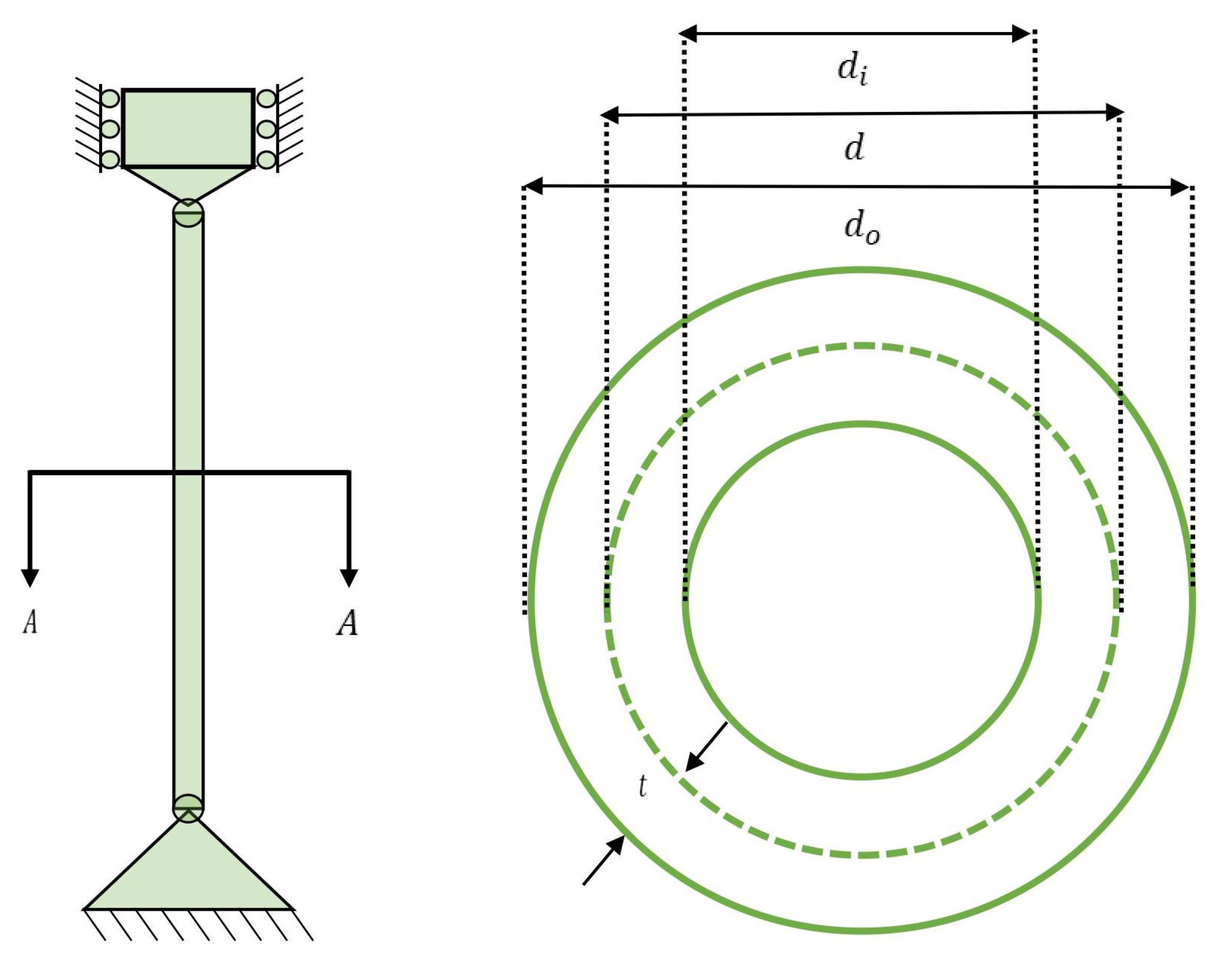
Appendix D.2. Pressure Vessel Design Problem (PVDP)
The mathematical model of the Pressure Vessel Design Problem (PVDP) is formulated in Equation (A2) and demonstrated in Figure A2.
Constraints:
Boundary constraints:
Figure A2.
Demonstration of the Pressure Vessel Design Problem (PVDP).
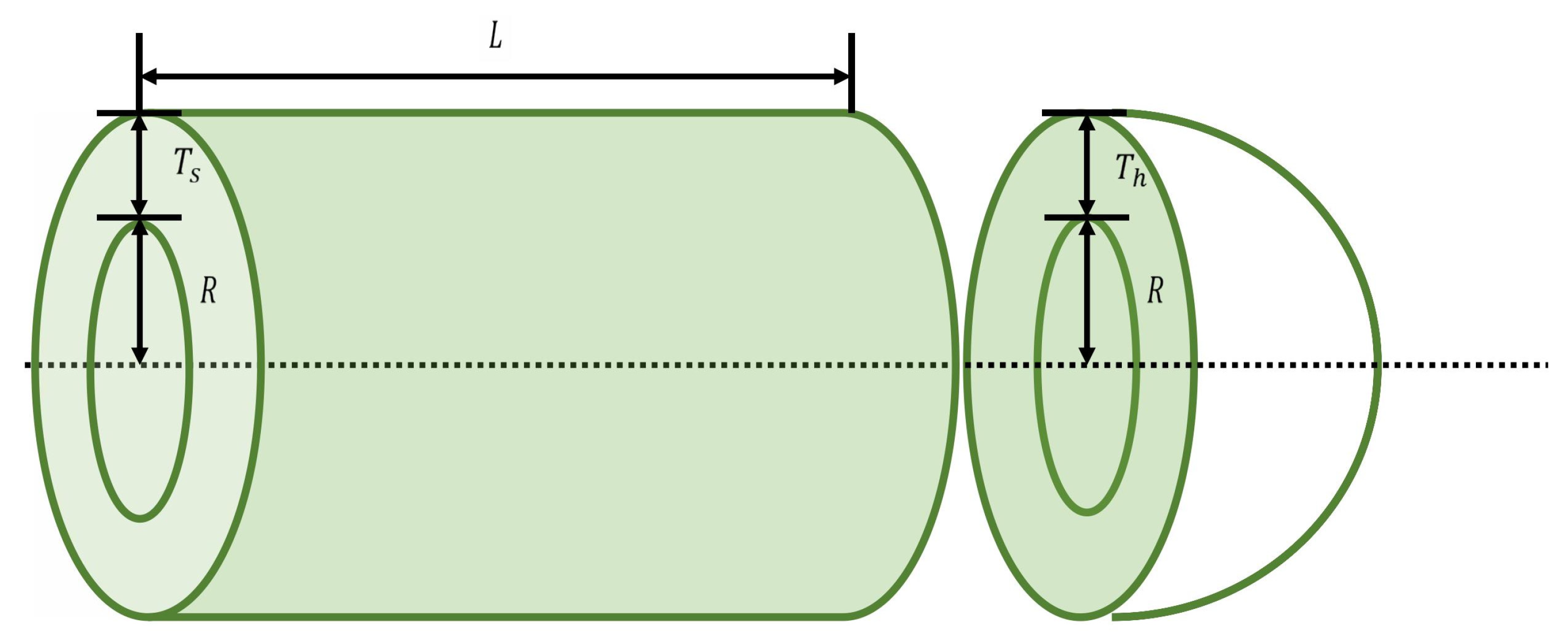
Appendix D.3. Piston Lever Design Problem (PLDP)
The mathematical model of the Piston Lever Design Problem (PLDP) is formulated in Equation (A3) and demonstrated in Figure A3.
Minimize:
subject to:
where
Figure A3.
Demonstration of the Piston Lever Design Problem (PLDP).
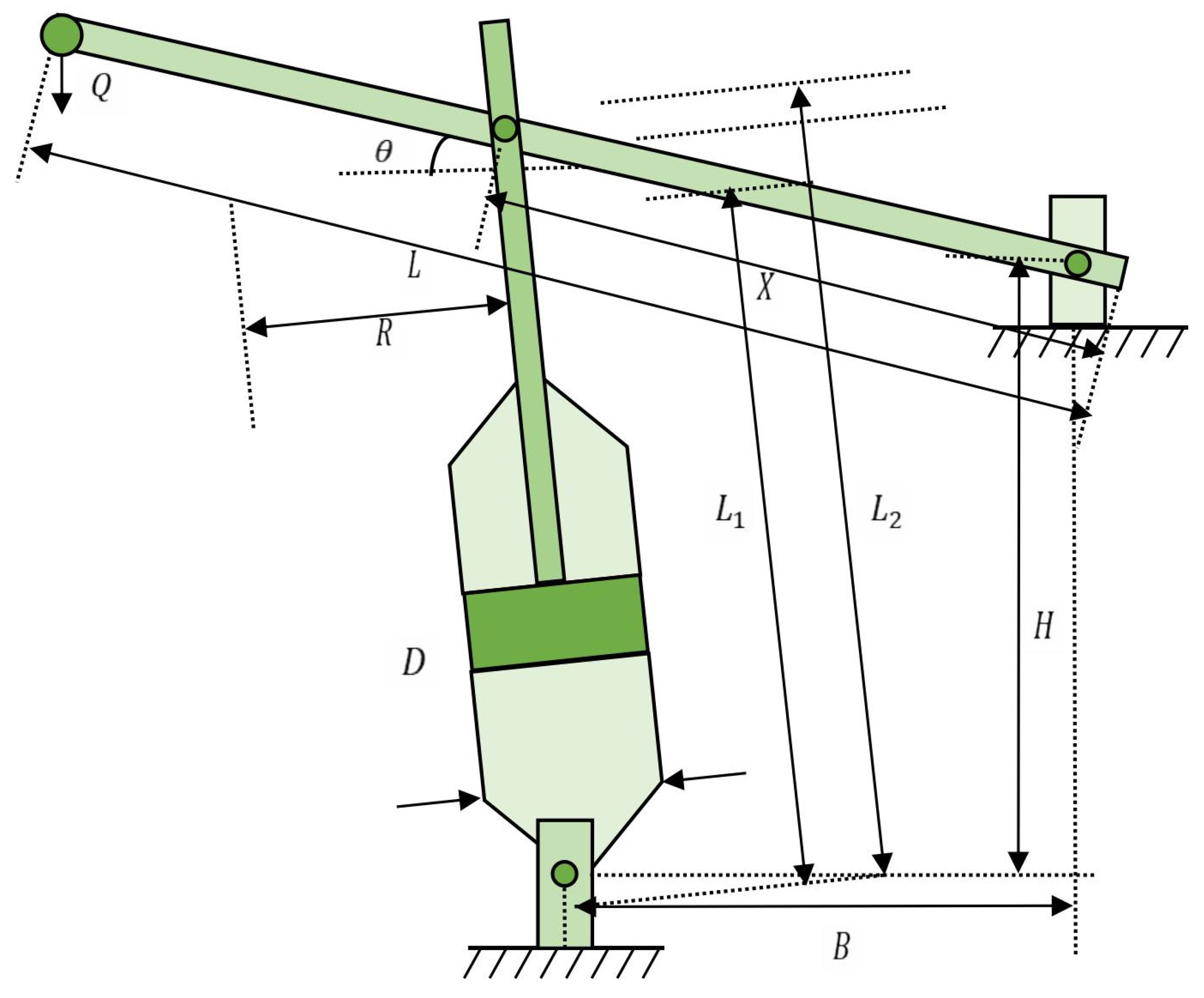
Appendix E. Experimental Results for Grounding Network Corrosion Diagnosis
8 × 8 Comparison Experiment Results for the Remaining Algorithms
Figure A4.
Results of the 8 × 8 comparison experiment for the remaining algorithms.
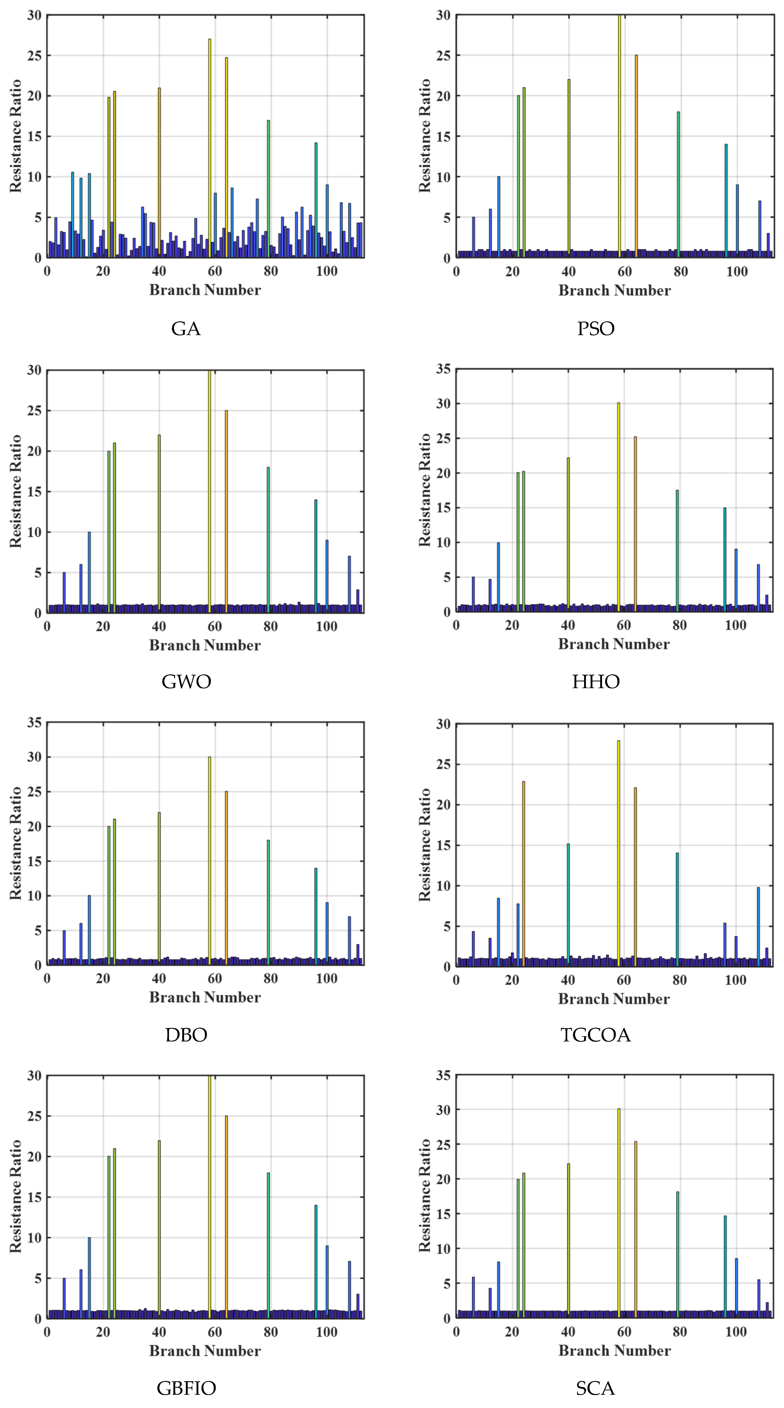
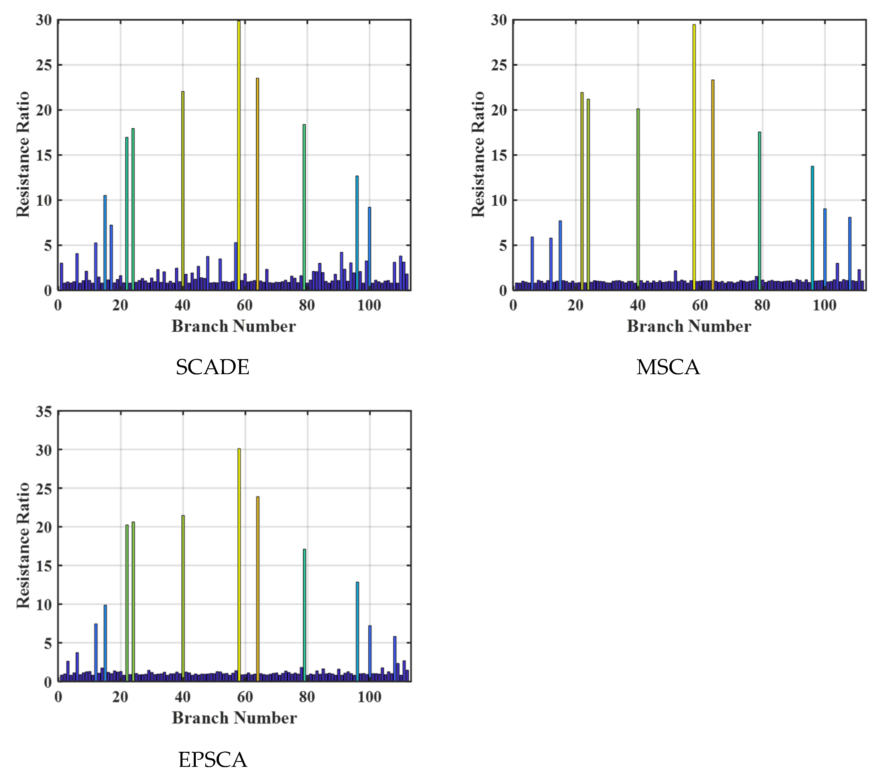
References
- Feng, Z.; Niu, W.; Cheng, C.; Zhou, J.; Yang, T. China’s hydropower energy system toward carbon neutrality. Front. Eng. Manag. 2022, 9, 677–682. [Google Scholar] [CrossRef] [Scilit]
- Xiong, B.; Zhou, L.; Ding, S. Study on dynamic characteristics of single-phase grounding fault of 1000 MW hydro generator under different grounding modes. Machines 2022, 10, 554. [Google Scholar] [CrossRef] [Scilit]
- Fotopoulou, M.; Rakopoulos, D.; Trigkas, D.; Stergiopoulos, F.; Blanas, O.; Voutetakis, S. State of the art of low and medium voltage direct current (DC) microgrids. Energies 2021, 14, 5595. [Google Scholar] [CrossRef] [Scilit]
- Zhang, C.; Liao, Y.; Gao, X.; Zhao, J.; Yuan, Y.; Liao, R. Research advances of soil corrosion of grounding grids. Micromachines 2021, 12, 513. [Google Scholar] [CrossRef] [Scilit]
- Qamar, A.; Al-Kharsan, I.H.; Uddin, Z.; Alkhayyat, A. Grounding grid fault diagnosis with emphasis on substation electromagnetic interference. IEEE Access 2022, 10, 15217–15226. [Google Scholar] [CrossRef] [Scilit]
- Lu, C.; Li, L.; Liu, Z.; Xu, C.; Xin, M.; Fu, G.; Wang, T.; Wang, X. Location and corrosion detection of tower grounding conductors based on electromagnetic measurement. Measurement 2022, 199, 111469. [Google Scholar] [CrossRef] [Scilit]
- Song, H.; Dong, H.; Wang, X.; Tang, L. Non-destructive diagnosis of grounding grids based on the electromagnetic induction impedance method. Meas. Sci. Technol. 2021, 32, 115901. [Google Scholar] [CrossRef] [Scilit]
- Yu, B.; Zhao, P.; Cai, Y.; Yuan, W.; Yu, J.; Tan, Y. On-site electrochemical detection of corrosion in substation grounding system. Energies 2024, 17, 3906. [Google Scholar] [CrossRef] [Scilit]
- Hu, H.; Fang, M.; Hu, F.; Zeng, S.; Deng, X. A new design of substation grounding based on electrolytic cathodic protection and on transfer corrosion current. Electr. Power Syst. Res. 2021, 195, 107174. [Google Scholar] [CrossRef] [Scilit]
- Duan, Q.; Li, S.; Yi, X.; Song, H. Design of a grounding grid corrosion detection device based on the electrical network method. In Proceedings of the 2021 International Conference on Information Control, Electrical Engineering and Rail Transit (ICEERT), Lanzhou, China, 30 October–1 November 2021; pp. 148–157. [Google Scholar]
- Huang, L.; Xiao, X.; Huang, M.; Zhang, Z.; Song, Y.; Guan, L. Research on grounding grid corrosion diagnosis based on genetic K-means algorithm. Energy Sci. Eng. 2025, 13, 3074–3087. [Google Scholar] [CrossRef] [Scilit]
- Chen, J.; Qi, J.; Ao, Y.; Wang, K.; Song, X. A solution method for non-linear underdetermined equation systems in grounding grid corrosion diagnosis based on an enhanced hippopotamus optimization algorithm. Biomimetics 2025, 10, 467. [Google Scholar] [CrossRef] [Scilit] [PubMed]
- Xie, H.; Yang, F.; Hua, M.; Liu, S.; Hu, J.; He, Y. Grounding grid corrosion detection based on mini-batch gradient descent and greedy method. AIP Adv. 2021, 11, 065034. [Google Scholar] [CrossRef] [Scilit]
- Van Thieu, N.; Mirjalili, S. MEALPY: An open-source library for latest meta-heuristic algorithms in Python. J. Syst. Archit. 2023, 139, 102871. [Google Scholar] [CrossRef] [Scilit]
- Zhong, R.; Wang, Z.; Zhang, Y.; Lian, J.J.; Yu, J.; Chen, H. Integrating competitive framework into differential evolution: Comprehensive performance analysis and application in brain tumor detection. Appl. Soft Comput. 2025, 174, 112995. [Google Scholar] [CrossRef] [Scilit]
- Jia, H.; Zhou, X.; Zhang, J. Thinking innovation strategy (TIS): A novel mechanism for metaheuristic algorithm design and evolutionary update. Appl. Soft Comput. 2025, 175, 113071. [Google Scholar] [CrossRef] [Scilit]
- Alhijawi, B.; Awajan, A. Genetic algorithms: Theory, genetic operators, solutions, and applications. Evol. Intell. 2024, 17, 1245–1256. [Google Scholar] [CrossRef] [Scilit]
- Kennedy, J.; Eberhart, R. Particle swarm optimization. In Proceedings of the ICNN’95 International Conference on Neural Networks, Perth, Australia, 27 November–1 December 1995; pp. 1942–1948. [Google Scholar]
- Storn, R.; Price, K. Differential evolution—A simple and efficient heuristic for global optimization over continuous spaces. J. Glob. Optim. 1997, 11, 341–359. [Google Scholar] [CrossRef] [Scilit]
- Mirjalili, S.; Mirjalili, S.M.; Lewis, A. Grey wolf optimizer. Adv. Eng. Softw. 2014, 69, 46–61. [Google Scholar] [CrossRef] [Scilit]
- Mirjalili, S.; Lewis, A. The whale optimization algorithm. Adv. Eng. Softw. 2016, 95, 51–67. [Google Scholar] [CrossRef] [Scilit]
- Mirjalili, S. The ant lion optimizer. Adv. Eng. Softw. 2015, 83, 80–98. [Google Scholar] [CrossRef] [Scilit]
- Xu, L.; Guo, T.; Lu, X.; Liu, X.; Chen, Z.; Hu, L.; Li, S.; Li, P.; Zou, F. Research on corrosion diagnosis for grounding grid based on improved seagull optimization algorithm. J. Electr. Power Sci. Technol. 2025, 40, 275–282. [Google Scholar]
- Mirjalili, S. SCA: A sine cosine algorithm for solving optimization problems. Knowl.-Based Syst. 2016, 96, 120–133. [Google Scholar] [CrossRef] [Scilit]
- Rizk-Allah, R.M.; Hassanien, A.E. A comprehensive survey on the sine–cosine optimization algorithm. Artif. Intell. Rev. 2023, 56, 4801–4858. [Google Scholar] [CrossRef] [Scilit]
- Gupta, S.; Su, R. Diversity-enhanced modified sine cosine algorithm and its application in solving engineering design problems. J. Comput. Sci. 2023, 72, 102105. [Google Scholar] [CrossRef] [Scilit]
- Deng, L.; Liu, S. A sine cosine algorithm guided by elite pool strategy for global optimization. Appl. Soft Comput. 2024, 164, 111946. [Google Scholar] [CrossRef] [Scilit]
- Wei, F.; Zhang, Y.; Li, J. Multi-strategy-based adaptive sine cosine algorithm for engineering optimization problems. Expert Syst. Appl. 2024, 248, 123444. [Google Scholar] [CrossRef] [Scilit]
- Ishtaiwi, A.; Al-Shamayleh, A.S.; Fakhouri, H.N. A Hybrid JADE–Sine Cosine Approach for Advanced Metaheuristic Optimization. Appl. Sci. 2024, 14, 10248. [Google Scholar] [CrossRef] [Scilit]
- Liu, J.; Bi, C.; Chen, H.; Heidari, A.A.; Chen, H. Triangular-based sine cosine algorithm for global search and feature selection. Sci. Rep. 2025, 15, 12992. [Google Scholar] [CrossRef] [Scilit]
- Hu, Z.; Zhang, Q.; Wang, Y.; Su, Q.; Xiong, Z. Research orientation and novelty discriminant for new metaheuristic algorithms. Appl. Soft Comput. 2024, 157, 111521. [Google Scholar] [CrossRef] [Scilit]
- Heidari, A.A.; Mirjalili, S.; Faris, H.; Aljarah, I.; Mafarja, M.; Chen, H. Harris hawks optimization: Algorithm and applications. Future Gener. Comput. Syst. 2019, 97, 849–872. [Google Scholar] [CrossRef] [Scilit]
- Xue, J.; Shen, B. Dung beetle optimizer: A new meta-heuristic algorithm for global optimization. J. Supercomput. 2023, 79, 7305–7336. [Google Scholar] [CrossRef] [Scilit]
- Gámez, M.G.M.; Vázquez, H.P. A novel swarm optimization algorithm based on hive construction by Tetragonula carbonaria builder bees. Mathematics 2025, 13, 2721. [Google Scholar] [CrossRef] [Scilit]
- Dehghani, M.; Aly, M.; Rodriguez, J.; Sheybani, E.; Javidi, G. A novel nature-inspired optimization algorithm: Grizzly bear fat increase optimizer. Biomimetics 2025, 10, 379. [Google Scholar] [CrossRef] [Scilit]
- Liu, X.J.; Wang, L.G. A sine cosine algorithm based on differential evolution. Chin. J. Eng. 2020, 42, 1674–1684. [Google Scholar]
- Shang, C.; Zhou, T.; Liu, S. Optimization of complex engineering problems using modified sine cosine algorithm. Sci. Rep. 2022, 12, 20528. [Google Scholar] [CrossRef] [Scilit]
- Yucel, M.; Bekdas, G.; Nigdeli, S.M.; Sevgen, S. Artificial neural network model for optimum design of tubular columns. Int. J. Theor. Appl. Mech. 2018, 3, 82–86. [Google Scholar]
- Yang, X.S.; Huyck, C.; Karamanoglu, M.; Khan, N. True global optimality of the pressure vessel design problem: A benchmark for bio-inspired optimization algorithms. Int. J. Bio-Inspired Comput. 2013, 5, 329–335. [Google Scholar] [CrossRef] [Scilit]
- Sergent, N.; Tirovic, M.; Voveris, J. Design optimization of an opposed piston brake caliper. Eng. Optim. 2014, 46, 1520–1537. [Google Scholar] [CrossRef] [Scilit]
- Hu, H.; Luo, R.; Fang, M.; Zeng, S.; Hu, F. A new optimization design for grounding grid. Int. J. Electr. Power Energy Syst. 2019, 108, 61–71. [Google Scholar] [CrossRef] [Scilit]
- Lu, D.; Tong, Q.K.; Wong, C.P. Mechanisms underlying the unstable contact resistance of conductive adhesives. IEEE Trans. Electron. Packag. Manuf. 1999, 22, 228–232. [Google Scholar] [CrossRef] [Scilit]
- Kuh, E.S.; Hajj, I.N. Nonlinear circuit theory: Resistive networks. Proc. IEEE 1971, 59, 340–355. [Google Scholar] [CrossRef]
- Tellegen, B.D.H. A general network theorem, with applications. Philips Res. Rep. 1952, 7, 256–269. [Google Scholar]
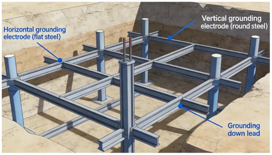
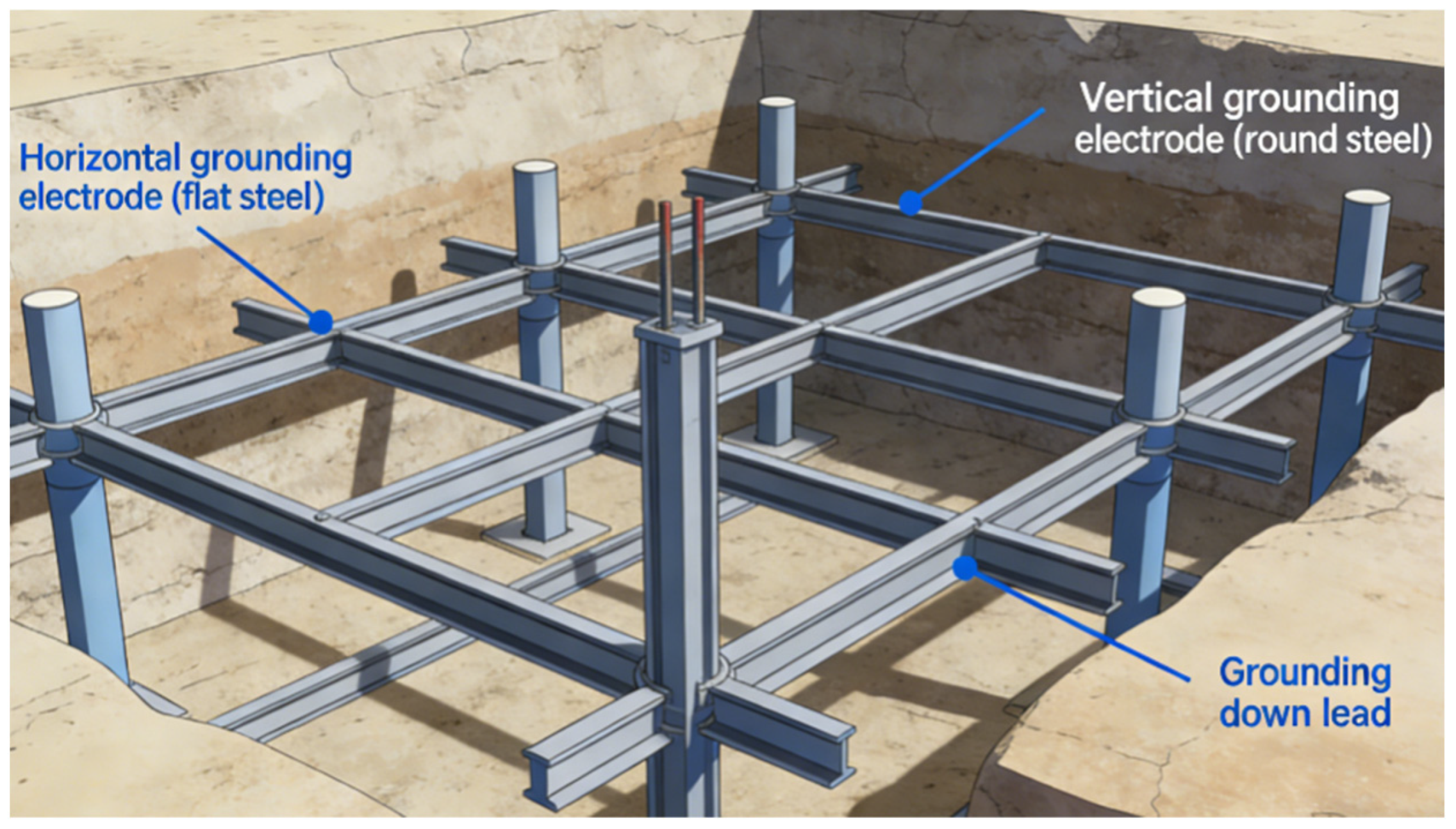
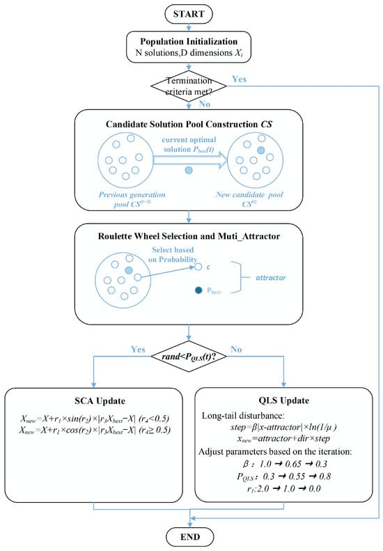
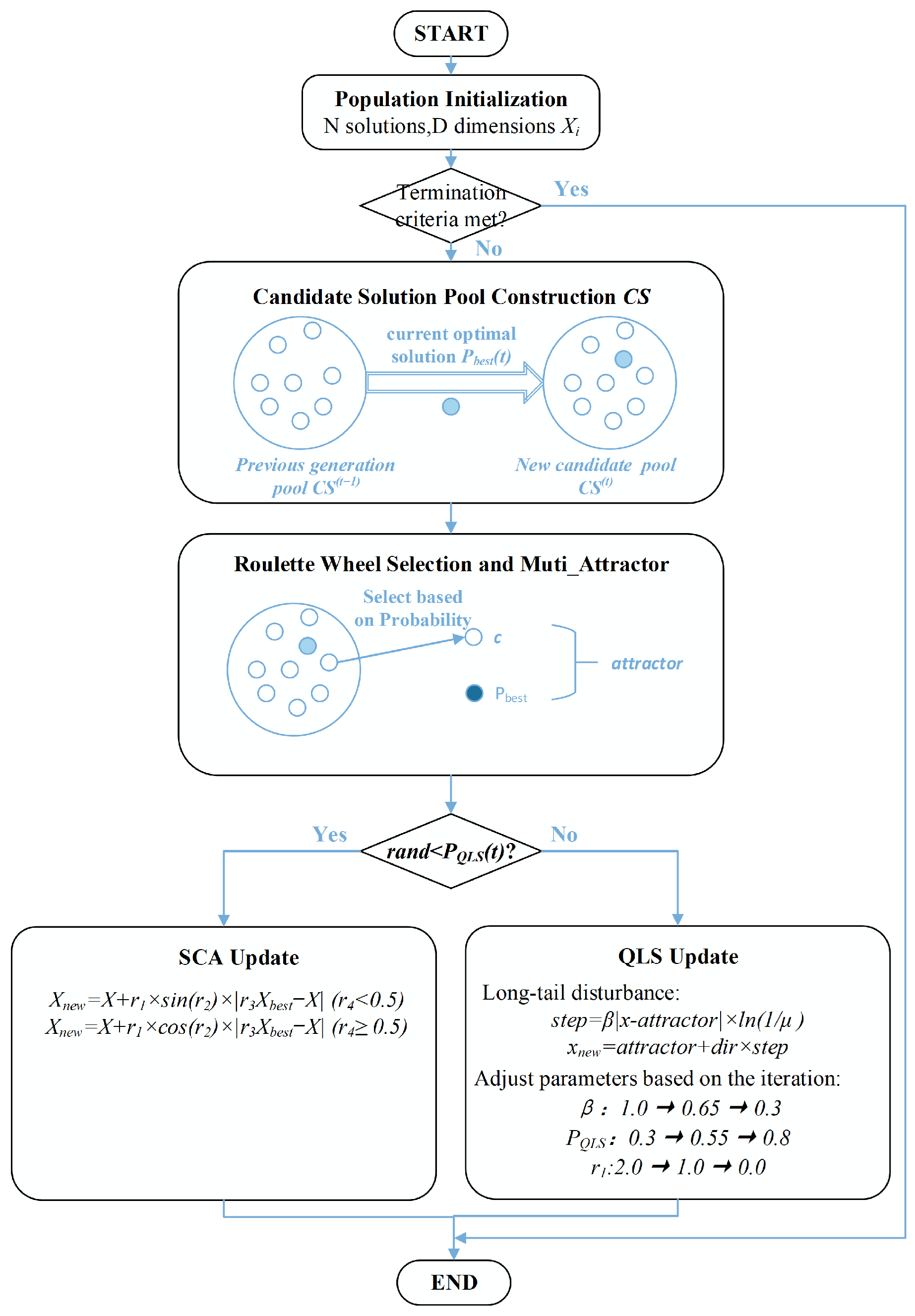
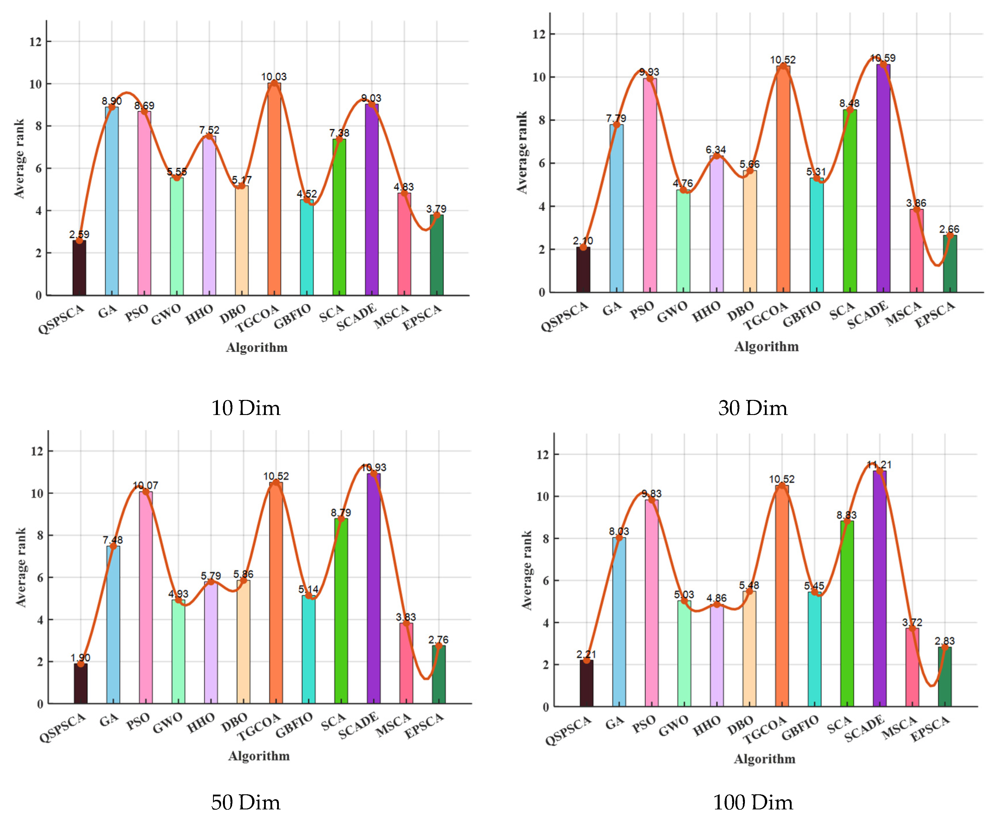
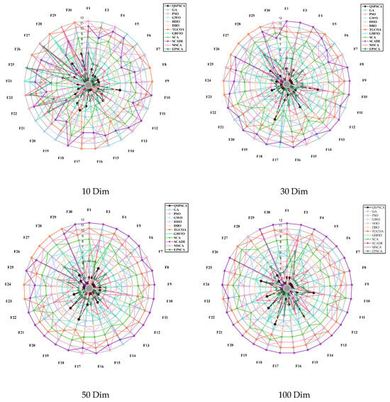
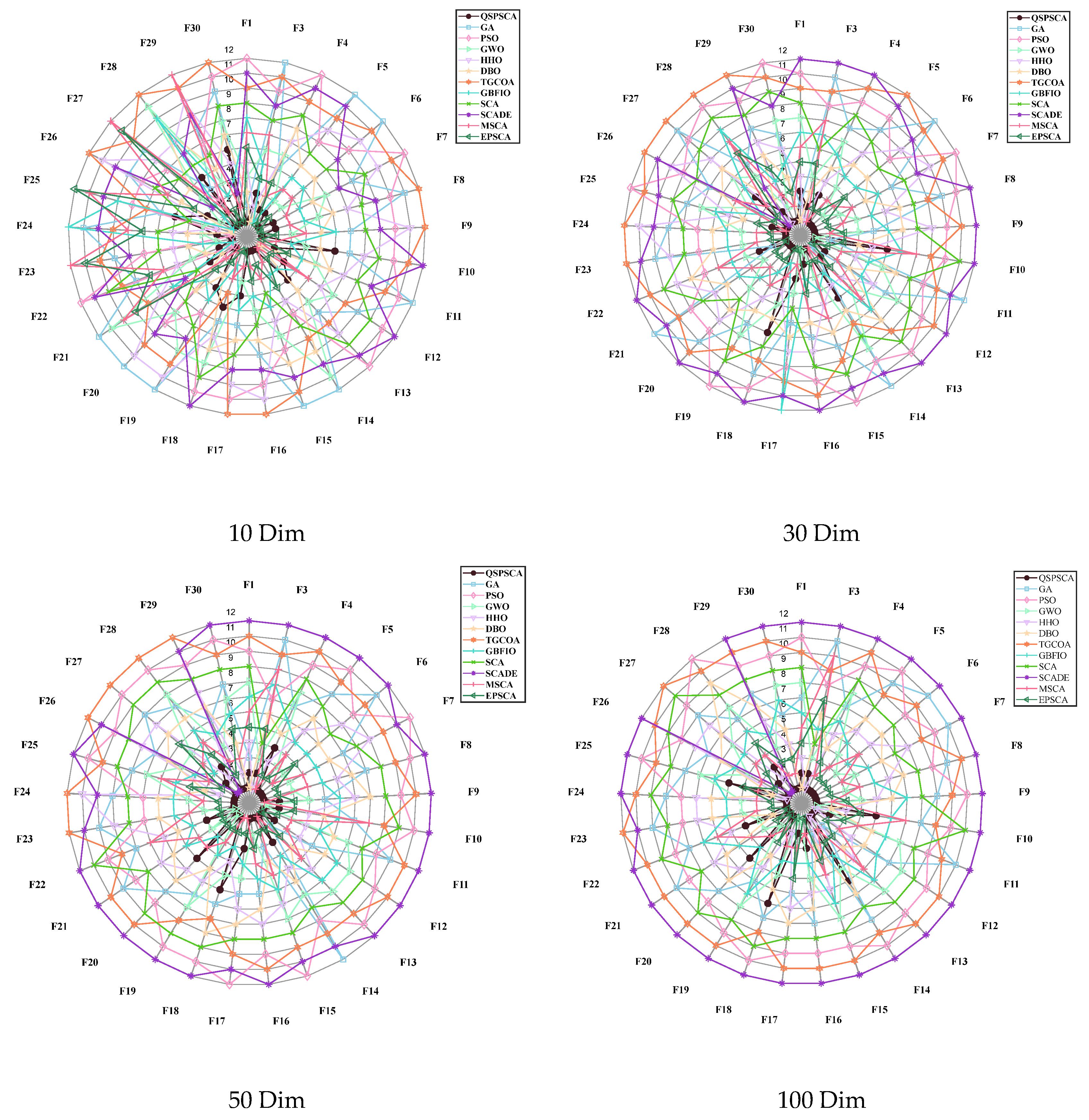
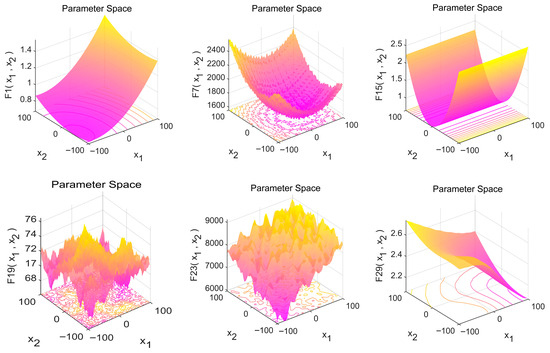
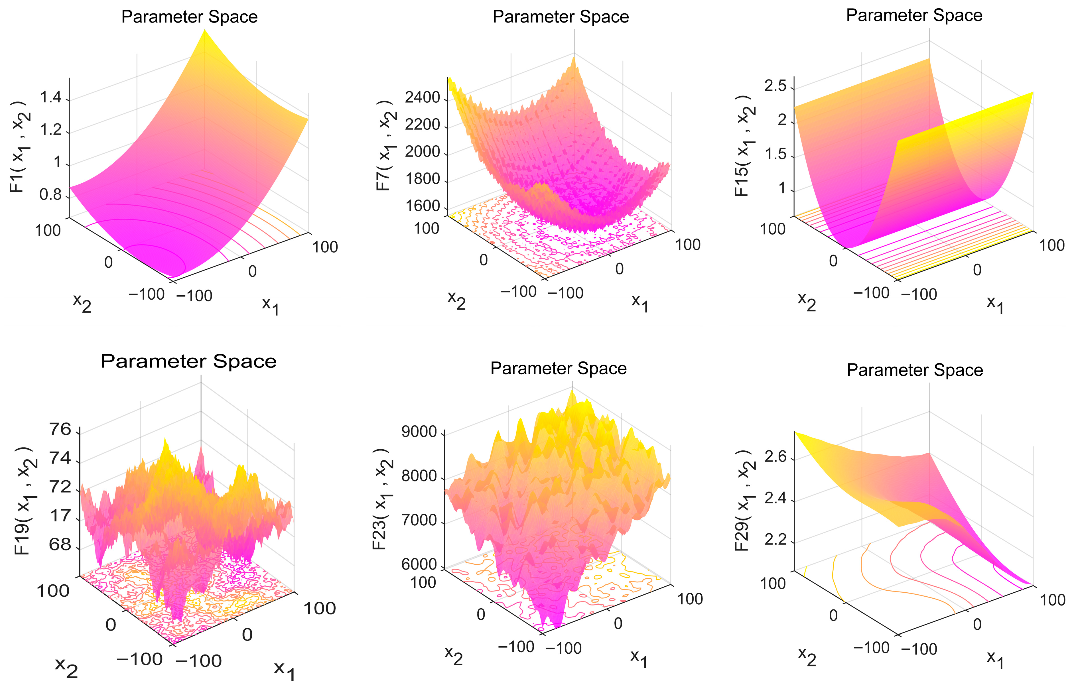
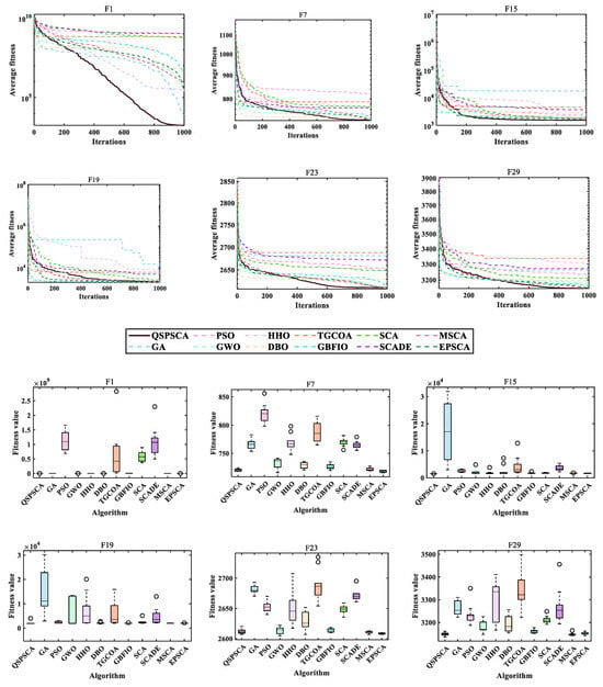
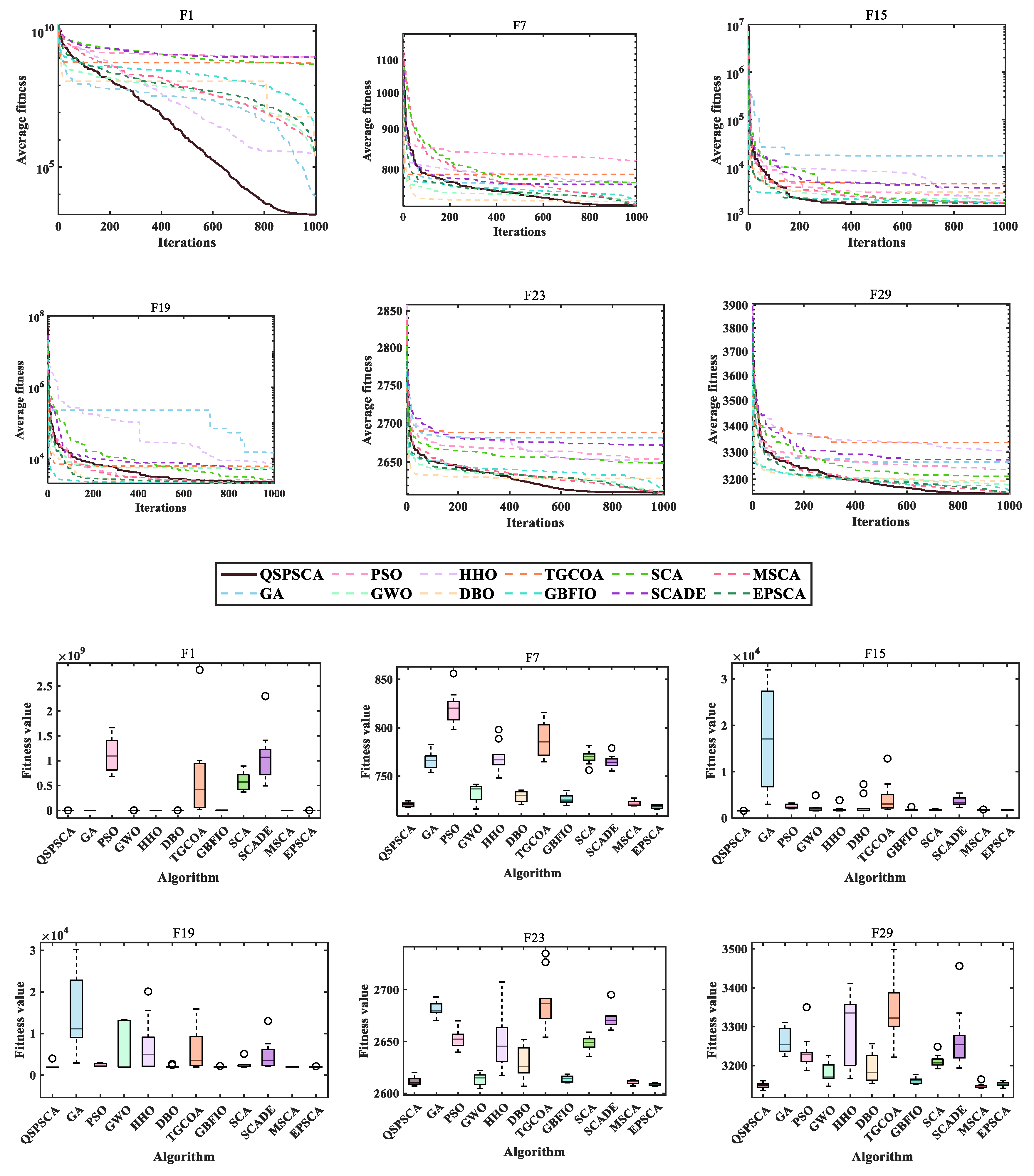
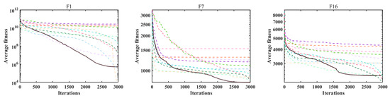
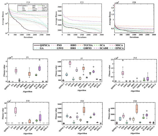
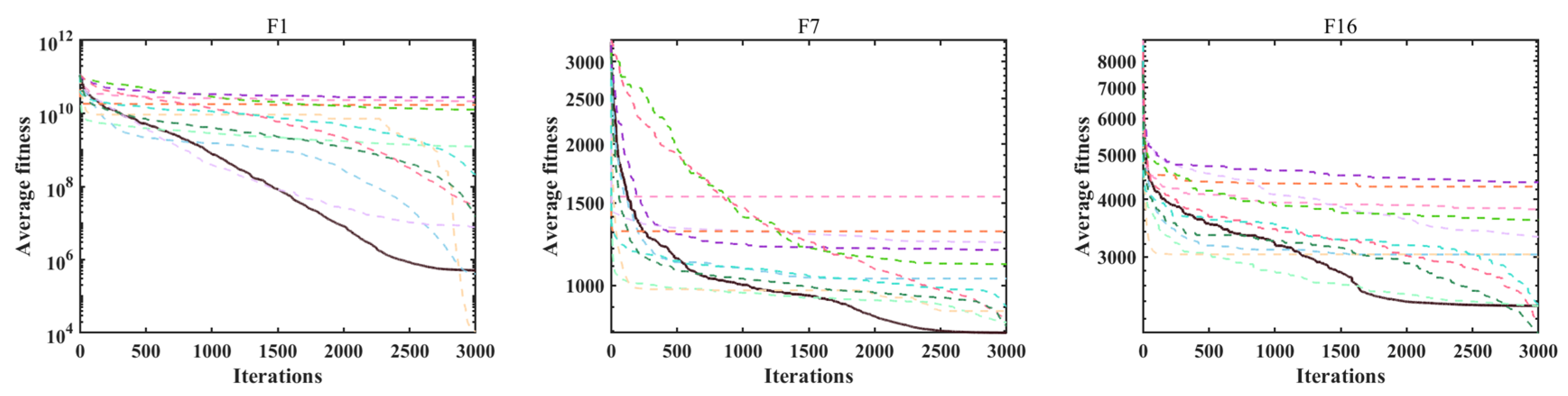
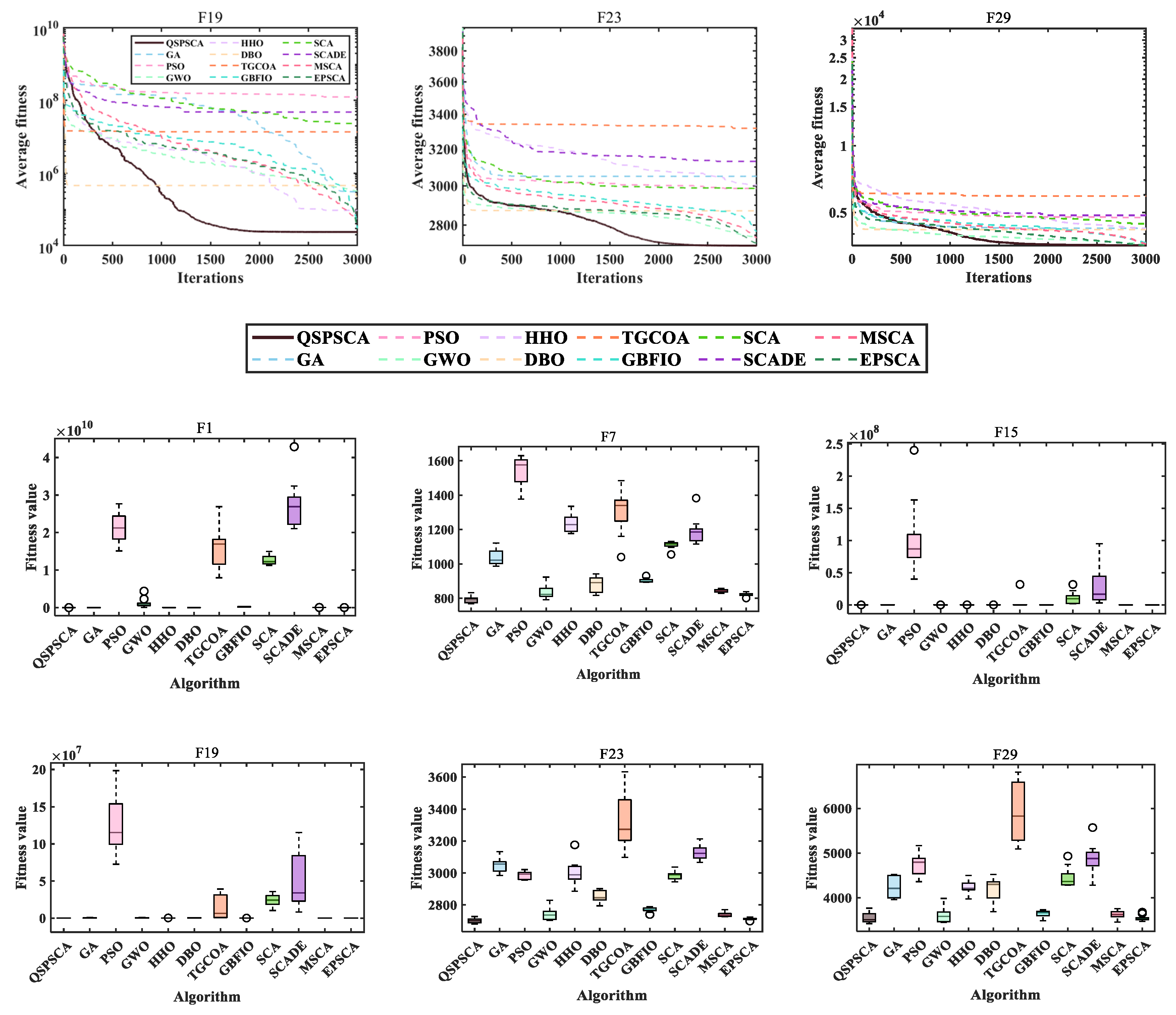
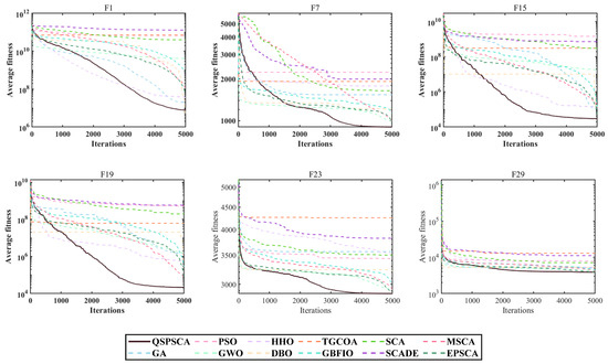
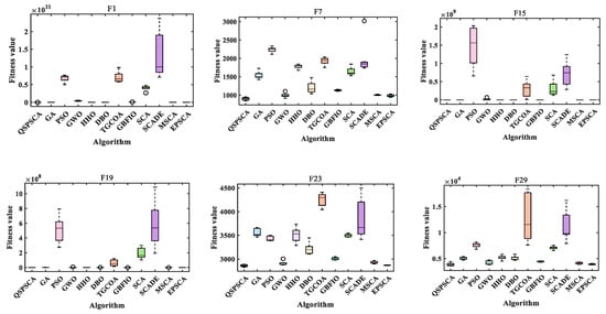
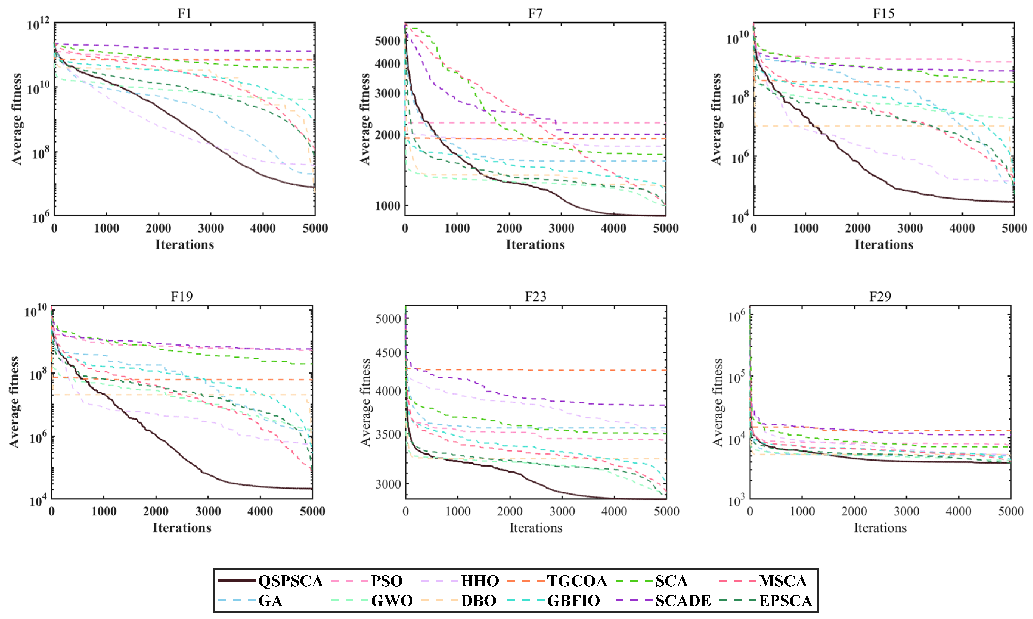
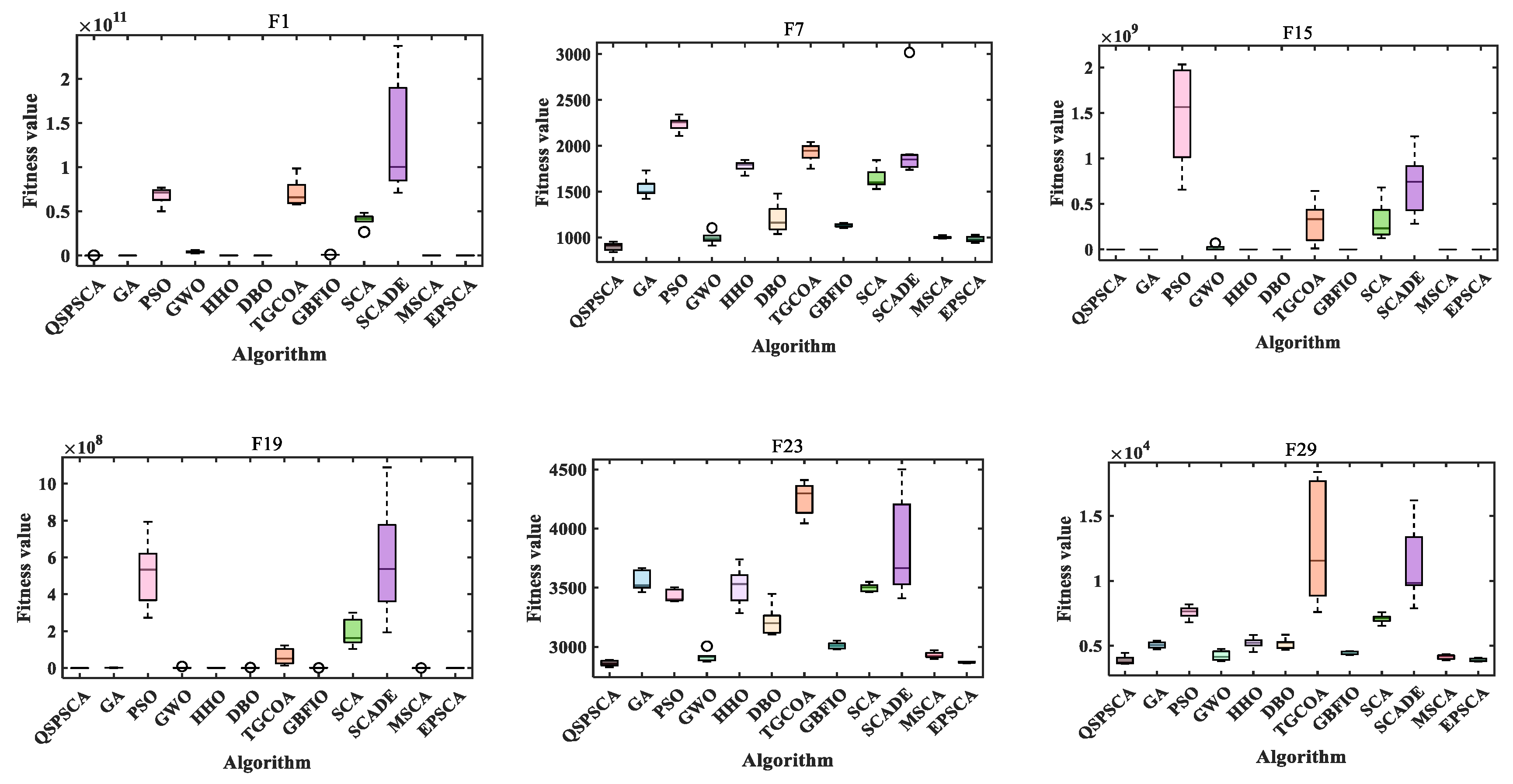
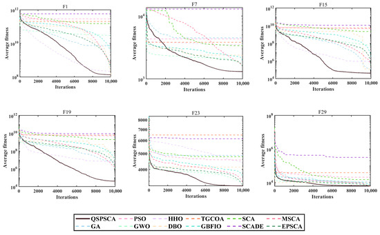
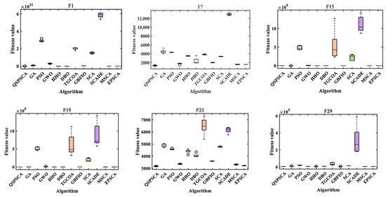
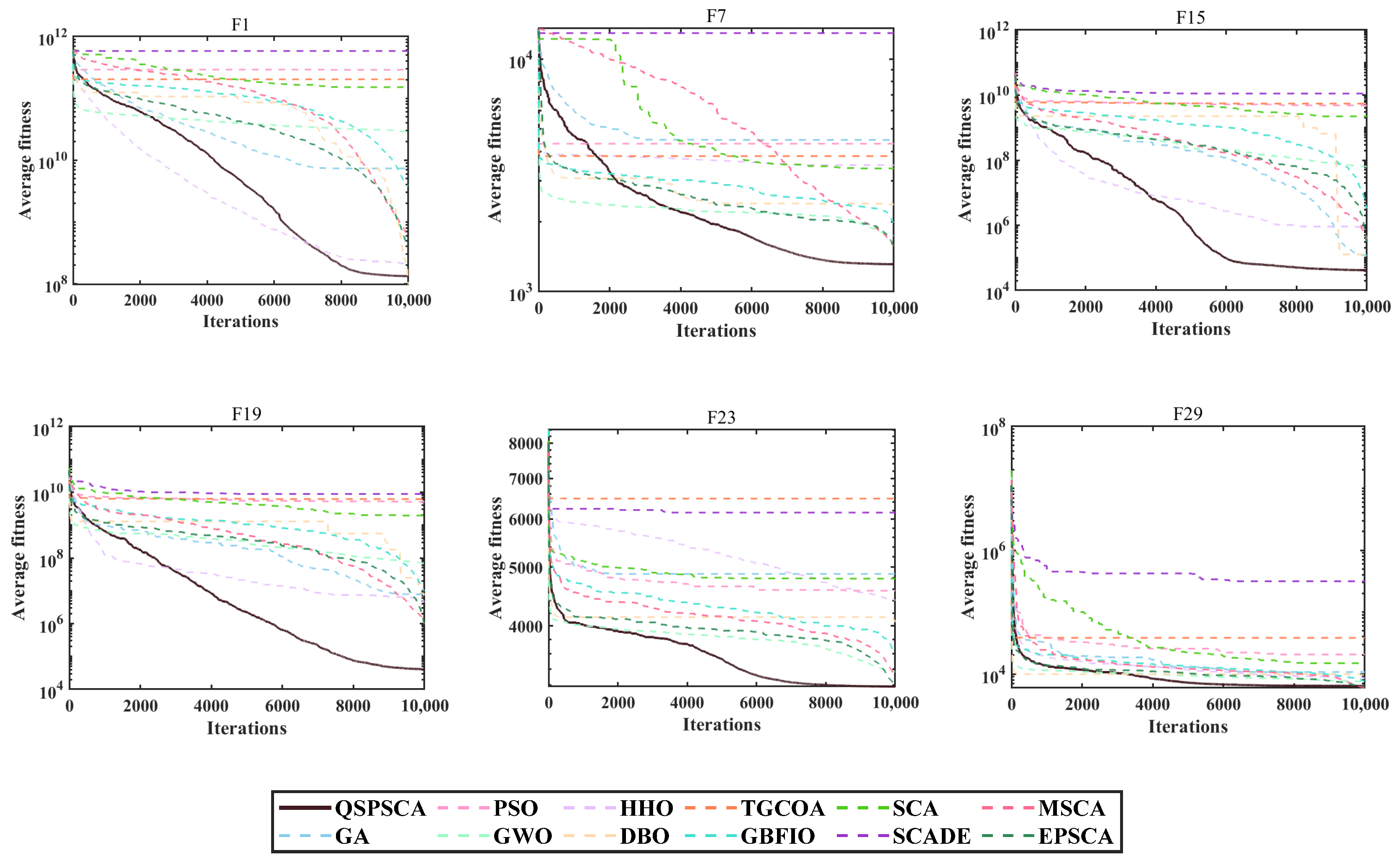
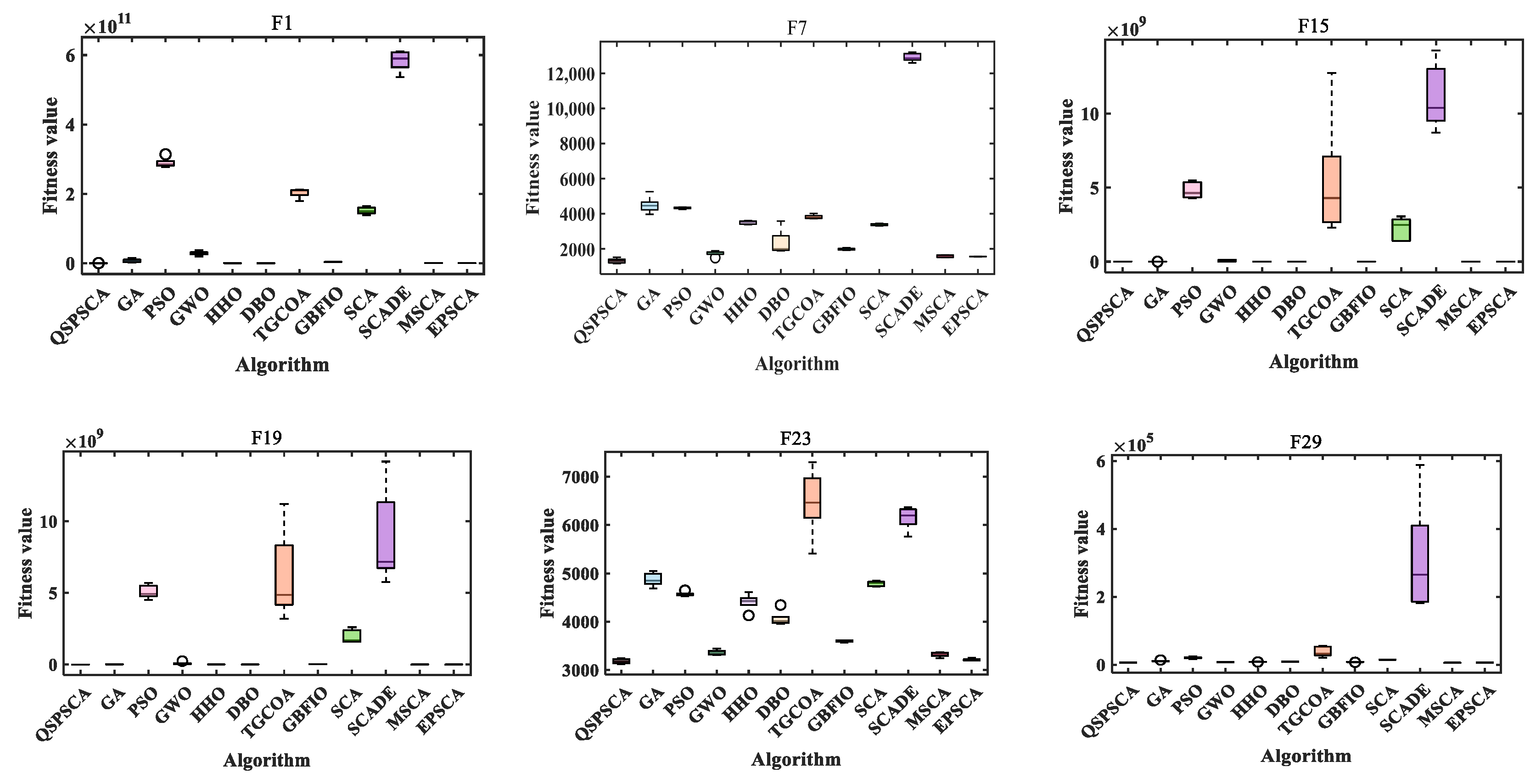
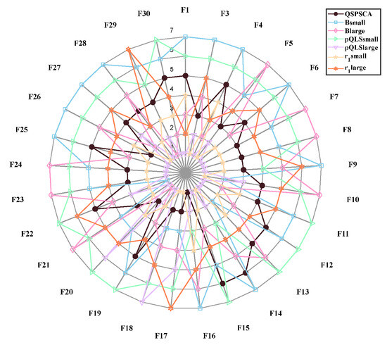
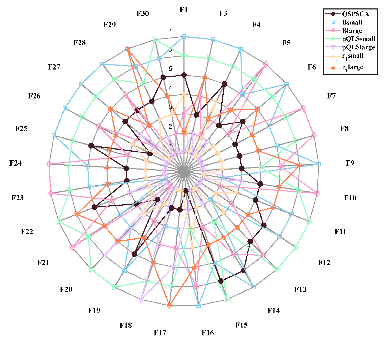
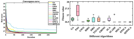
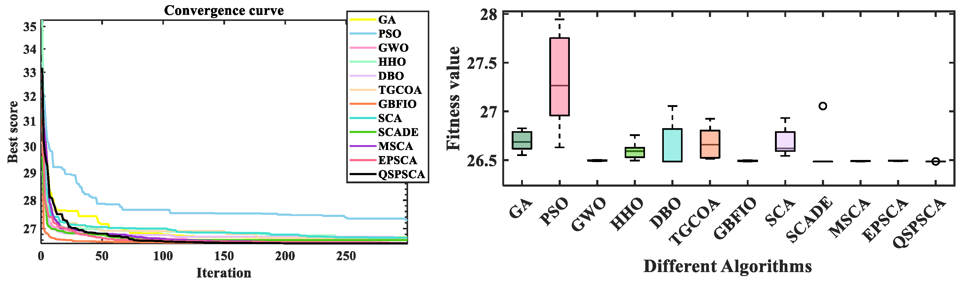
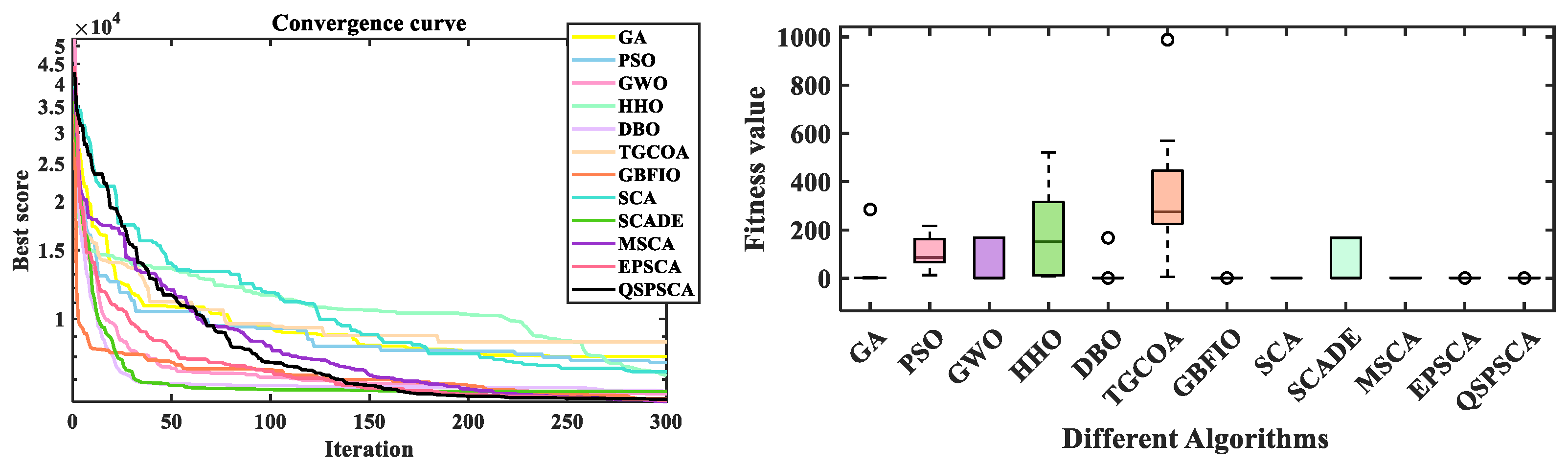
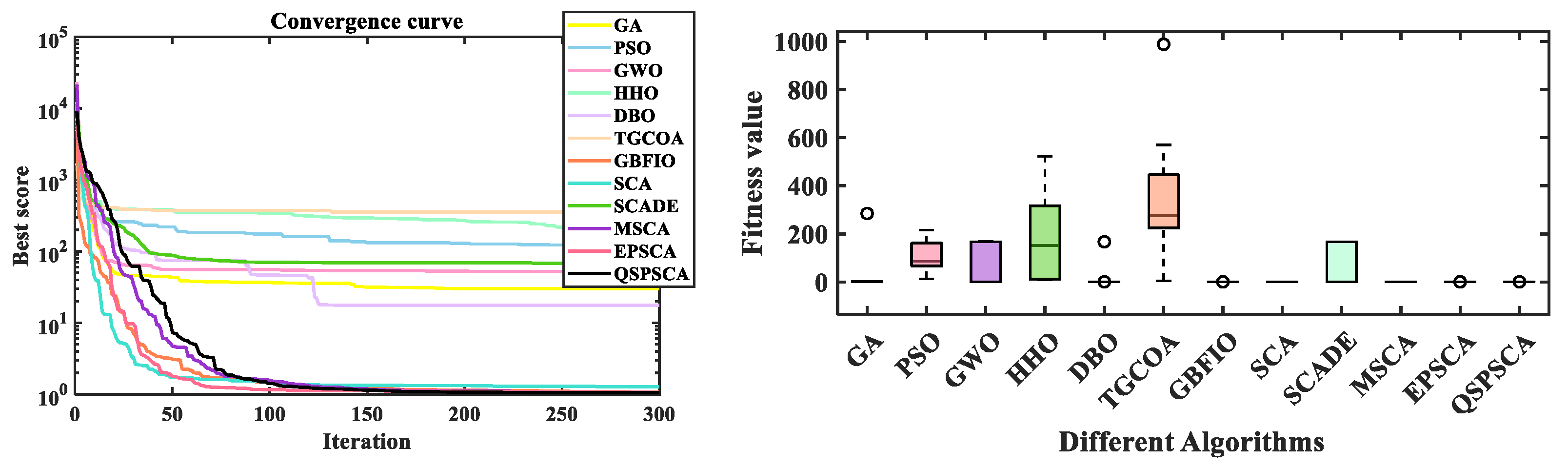
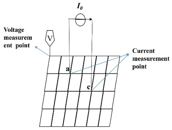
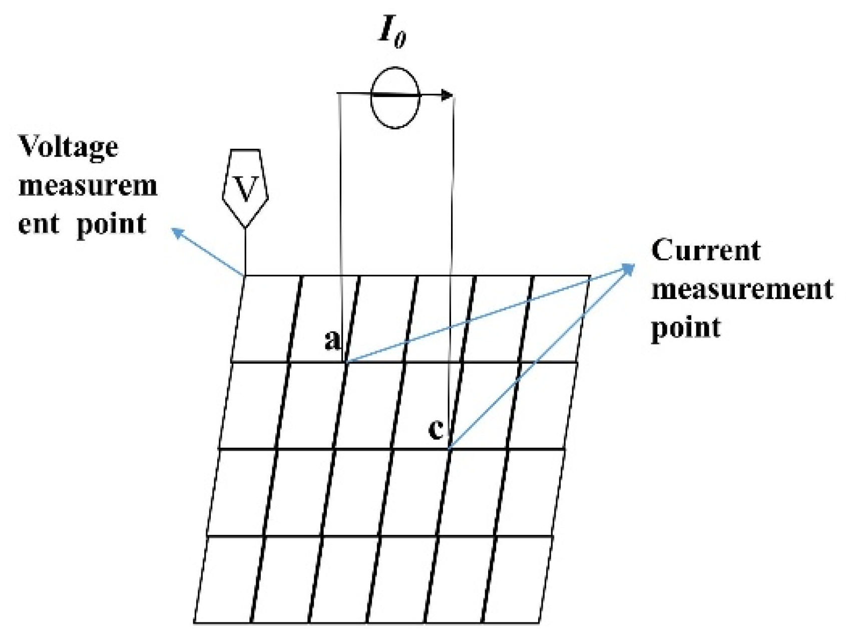
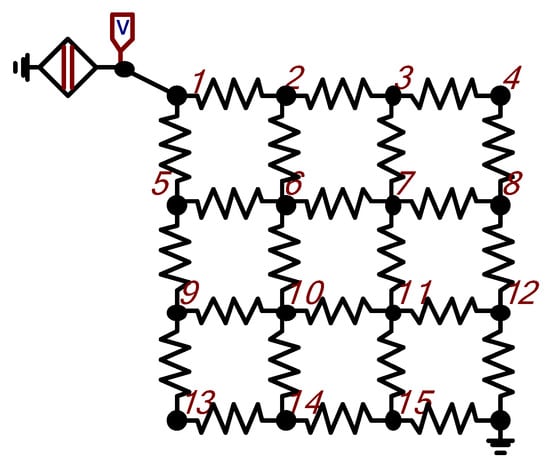
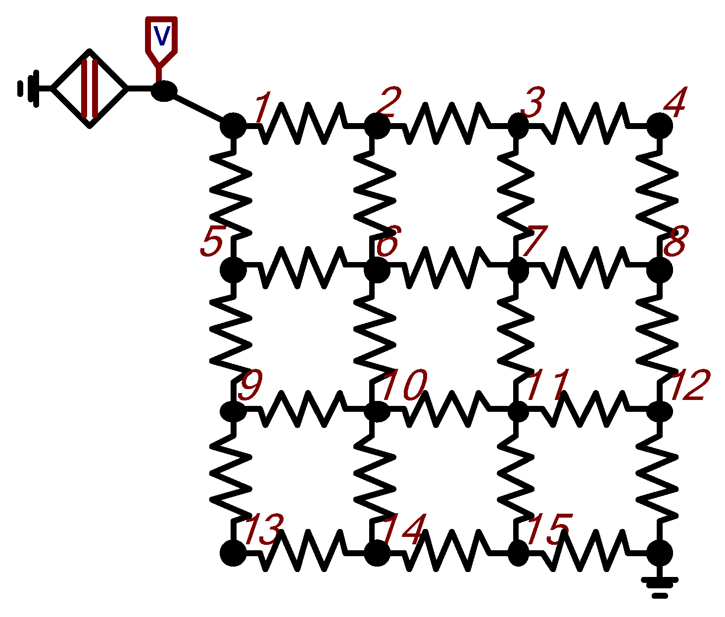
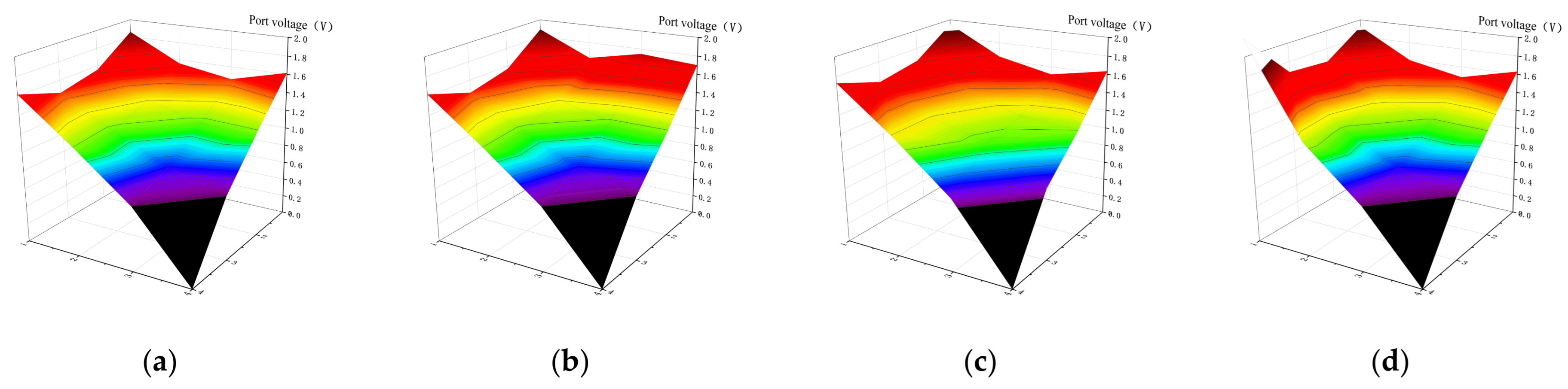
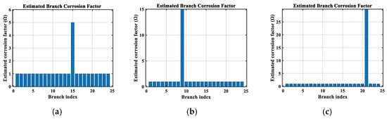
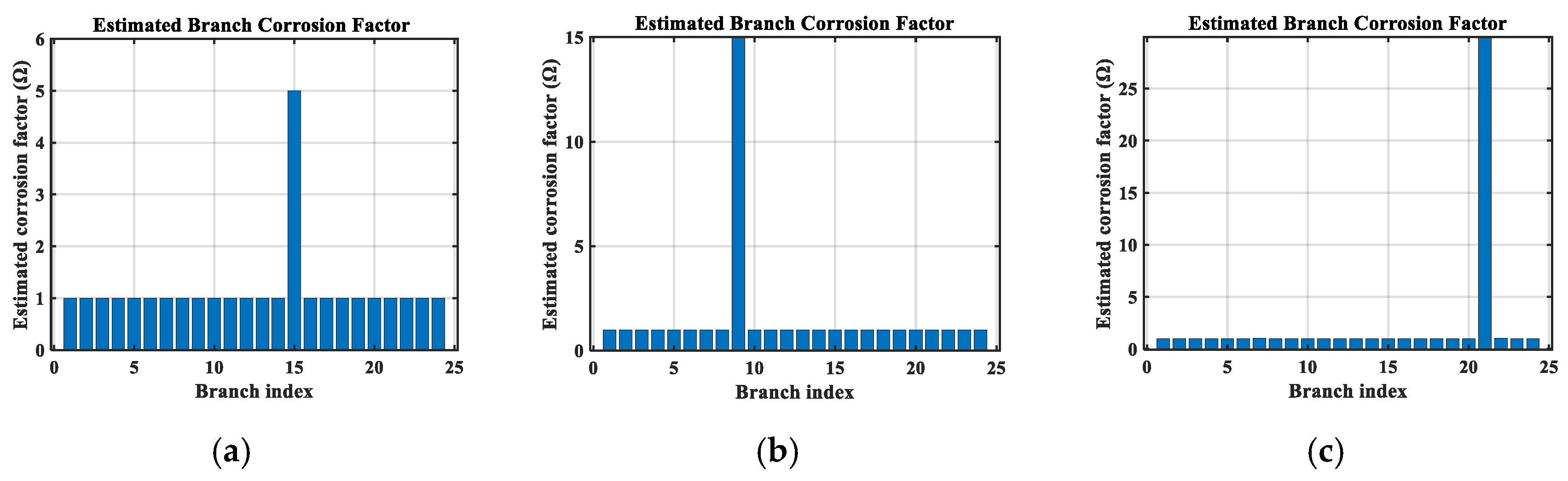
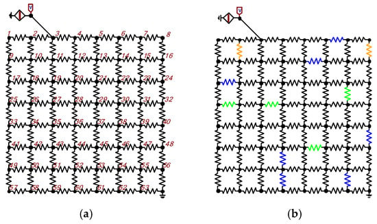
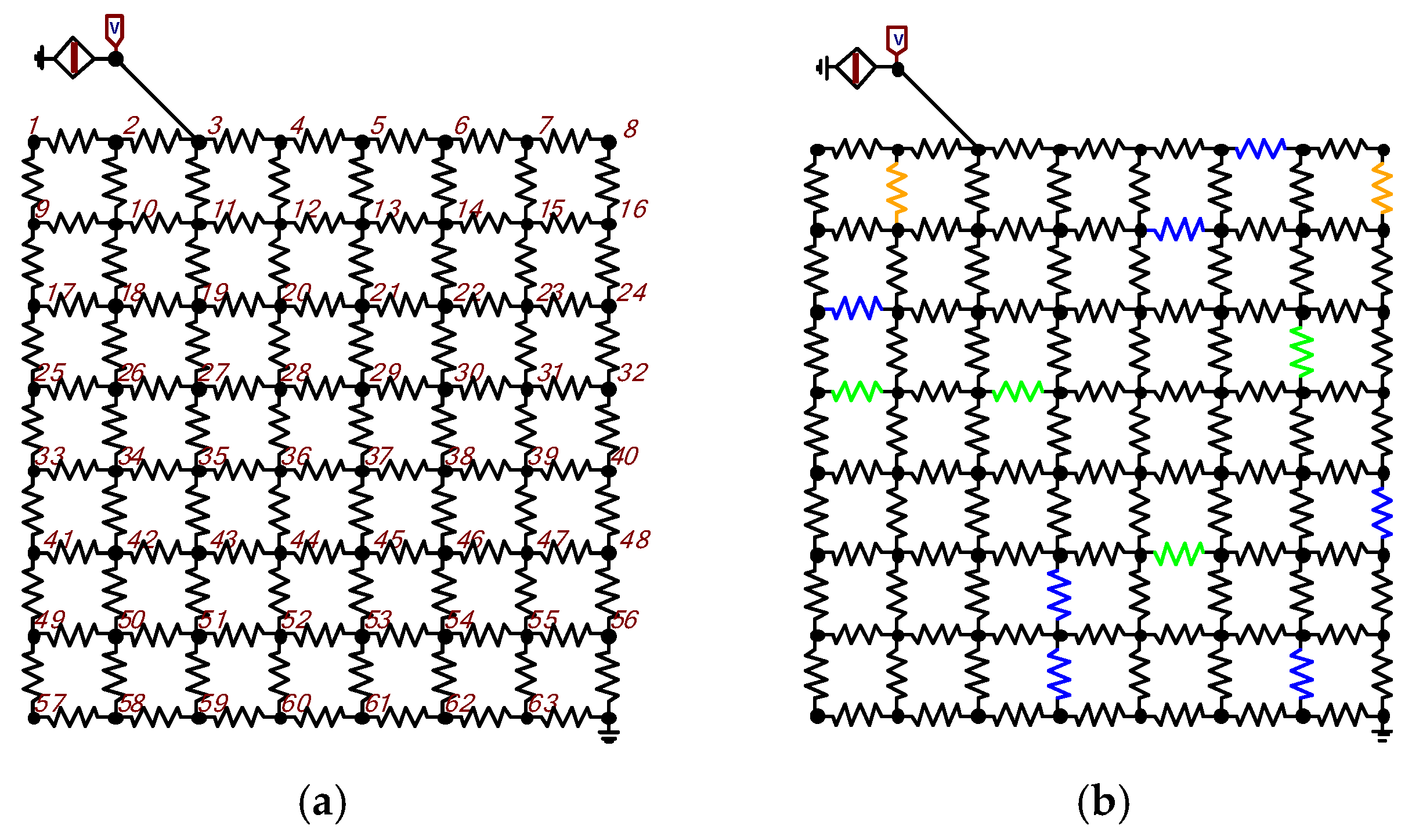
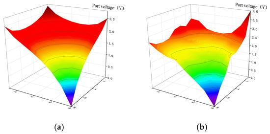
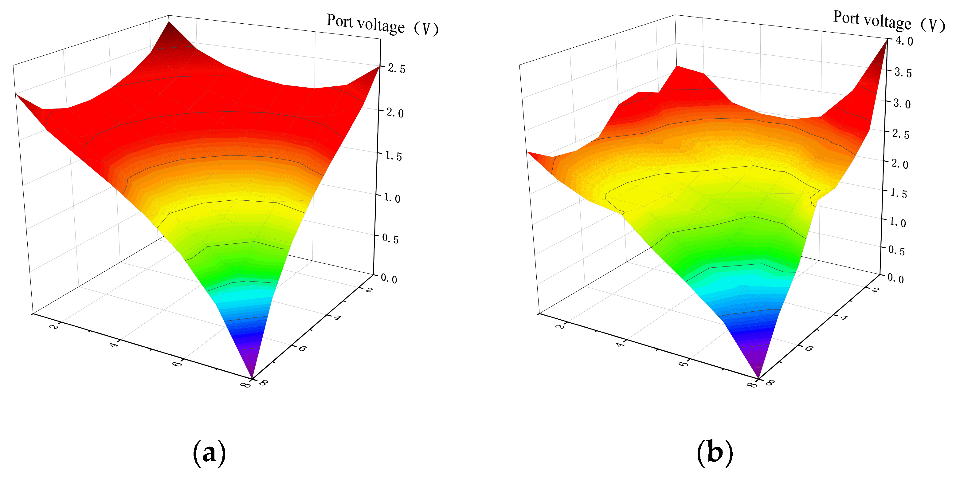
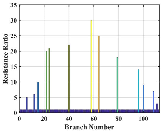
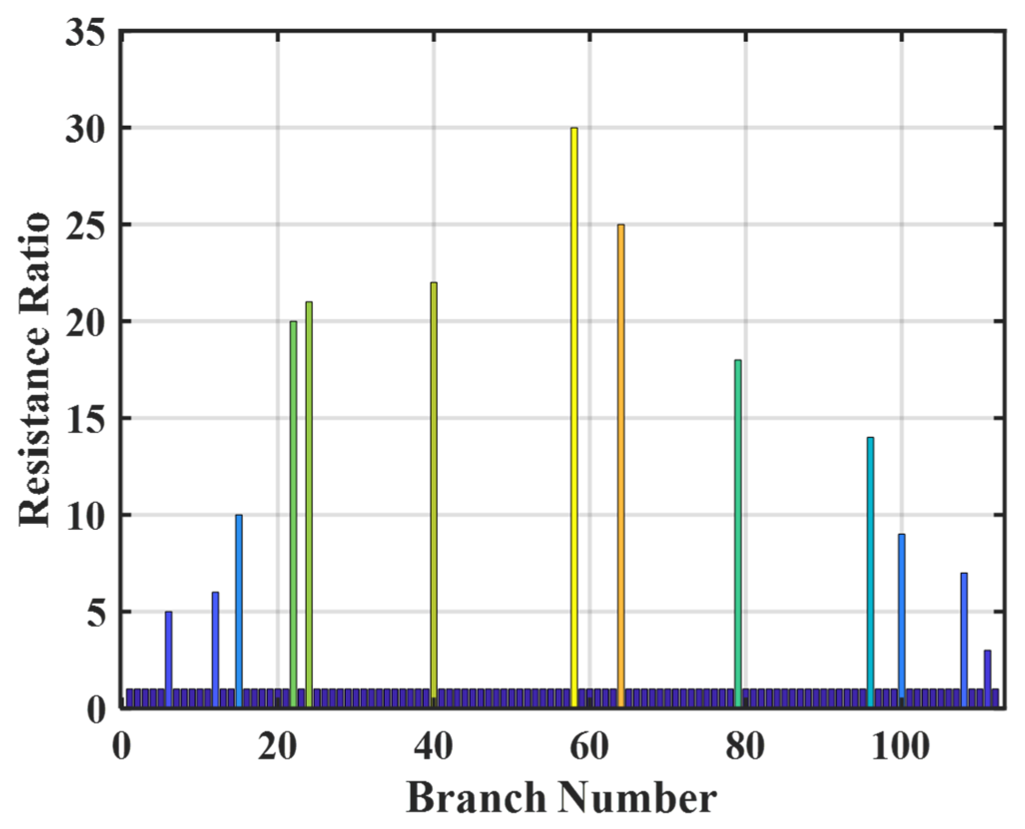

Disclaimer/Publisher’s Note: The statements, opinions and data contained in all publications are solely those of the individual author(s) and contributor(s) and not of MDPI and/or the editor(s). MDPI and/or the editor(s) disclaim responsibility for any injury to people or property resulting from any ideas, methods, instructions or products referred to in the content. |
© 2026 by the authors. Licensee MDPI, Basel, Switzerland. This article is an open access article distributed under the terms and conditions of the Creative Commons Attribution (CC BY) license.