


Abstract
The modeling and control of photovoltaic and other engineering systems highly depend on the accuracy of parameter identification. However, parameter extraction for photovoltaic equivalent models typically presents a high-dimensional, strongly nonlinear, and multimodal global optimization problem. Traditional analytical or gradient-based methods are sensitive to initial values and easily fall into local optima. To address this issue, this paper proposes a multi-strategy improvement teaching–learning-based optimization algorithm (SNTLBO). A social learning network structure with symmetric interaction topology is introduced into the classical TLBO framework to characterize the knowledge propagation relationships among individuals. Through this symmetric and balanced information exchange mechanism, learners can be guided not only by the teacher but also by multiple neighbors within the network, enabling more diverse and symmetric exploration of the search space and enhancing population diversity and global search capability. Furthermore, a teacher reputation mechanism is constructed, where historical performance is used to weight teacher influence, strengthening the guidance of high-quality solutions and accelerating convergence. Meanwhile, an adaptive teaching factor is designed to dynamically adjust the teaching intensity based on the distance between the teacher and students in the solution space, maintaining a dynamic balance (symmetry) between exploration and exploitation. To evaluate the performance of the proposed algorithm, SNTLBO is systematically compared with 11 advanced optimization algorithms on two benchmark test suites, CEC2017 (30D, 50D) and CEC2022 (10D, 20D). Non-parametric statistical tests are conducted to assess significance. The results demonstrate that SNTLBO shows competitive advantages in terms of convergence speed, solution accuracy, and stability. Finally, SNTLBO is applied to the parameter estimation of single-diode, double-diode, triple-diode, quadruple-diode, and photovoltaic module models. Experimental results show that the proposed algorithm achieves higher identification accuracy and robustness in terms of RMSE, IAE, and I–V/P–V curve fitting, verifying its effectiveness and practical value for complex global optimization and practical engineering applications.
1. Introduction
With the continuous development of the global economy and the constant advancement of technology, humanity’s demand for energy is growing rapidly. The large-scale use of traditional fossil fuels not only exacerbates resource depletion but also has a serious impact on the ecological environment and climate system. Against this backdrop, achieving coordinated development between economic growth and environmental protection has become a crucial issue facing all countries. The concept of sustainable development provides important guidance for addressing issues such as energy security, environmental protection, and social equity [1,2]. Its core lies in promoting the development and utilization of clean energy and building a low-carbon, efficient, and sustainable energy system [3,4,5].
Among various renewable energy technologies, photovoltaic power generation is considered an important component of the future energy structure transformation due to its abundant resources, cleanliness, environmental friendliness, and strong scalability. The performance evaluation, operation control, and optimal design of photovoltaic systems largely depend on the accuracy of their mathematical models, and the precise identification of model parameters is crucial for ensuring the reliability of simulations and predictions [6,7]. However, the output characteristics of photovoltaic cells are significantly affected by environmental factors such as irradiance and temperature, and their equivalent models typically exhibit strong nonlinear characteristics, making the parameter extraction process highly complex and uncertain [8,9,10].
The extraction of photovoltaic model parameters is essentially a high-dimensional, nonlinear, and multi-modal optimization problem. Traditional analytical methods and gradient-based optimization techniques are often sensitive to initial conditions and prone to getting stuck in local optima, making it difficult to obtain satisfactory results in complex search spaces [11,12]. This, to some extent, limits their widespread application and effectiveness in practical engineering applications.
To overcome the aforementioned shortcomings, researchers have gradually introduced heuristic and intelligent optimization algorithms into the field of photovoltaic model parameter identification. These methods, by simulating natural evolutionary mechanisms or group collaborative behaviors, demonstrate significant advantages in global search capability and robustness, effectively improving parameter identification accuracy and algorithm stability. For example, Imade Choulli et al. proposed an enhanced version of the JAYA algorithm for accurate extraction of equivalent model parameters by introducing individual weighting factors and the current population average into the traditional JAYA equation [13]. Experiments showed that this algorithm performs better in photovoltaic parameter estimation problems, particularly in terms of stability, accuracy, and convergence speed, when applied to single-diode, double-diode, triple-diode, and photovoltaic models. Mehar-Un-Nisa Khursheed et al. proposed an improved pollen pollination algorithm for accurate estimation of PV cell and module parameters [14]. Evaluated using seven benchmark functions and three case studies, the experimental results showed that the algorithm avoids premature convergence and stagnation in local optima, a problem faced by traditional FPA, and achieves more reliable and efficient results. Tummala S. L. V. Ayyarao et al. proposed a novel metaheuristic optimization algorithm inspired by ancient war strategies and based on the strategic movements of armies during wartime [15], which was used for parameter estimation of solar photovoltaic models. Experimental results demonstrated that this algorithm exhibited superior performance compared to state-of-the-art algorithms. Therefore, exploring efficient and reliable heuristic optimization strategies for the accurate extraction of photovoltaic model parameters is of great theoretical significance and engineering value for improving the accuracy of photovoltaic system modeling and promoting the development of renewable energy technologies.
Teaching–learning-Based Optimization (TLBO) is a heuristic algorithm proposed by R.V. Rao et al., based on the influence of teachers on learners [16]. It divides the optimization process into a teacher phase and a learner phase, with both phases working together to achieve good results. TLBO was tested on five constrained benchmark functions with different characteristics, four different benchmark mechanical design problems, and six mechanical design optimization problems with practical applications, and it consistently achieved good experimental results. Mohammadhossein Dastan et al. combined TLBO with the charged system search algorithm to propose a hybrid algorithm [17]. Experiments on several benchmark truss structures showed that this algorithm improved the convergence rate and quickly obtained optimal and ideal designs. Sumit Kumar et al. proposed a novel multi-objective teaching–learning optimization algorithm based on non-dominated sorting and a solution archiving framework [18]. Experimental results on five complex optimization problems with discrete design variables and multiple constraints show that MOTLBO demonstrates promise with its coherence and diversification of solutions for producing the desired Pareto fronts. Wu et al. combined reinforcement learning with heuristic algorithms to propose an improved teaching–learning-based optimization algorithm [19]. Experiments on 23 standard benchmark functions, 8 CEC2017 test functions, and eight industrial engineering design problems showed that RLTLBO has superior performance and promising prospects in handling real-world optimization problems.
In 2025, Mohammad Azim Eirgash proposed a novel Super Oppositional Learning (SOL) strategy to improve the Time–Cost–Quality–CO2 Emission Problem [20], called the Super Oppositional Teaching Optimization Algorithm. Experiments showed that SOTLBO outperformed the comparative algorithms, achieving the highest excess value (HV) across 33 activities. In 2026, Tao Han et al. proposed an Adaptive Quantization (ATLBO-Q) framework based on Teaching–learning Optimization (TLBO) for minimum mean square error MIMO detectors [21]. Through an adaptive teacher-learning phase, code width assignment is iteratively optimized, avoiding a complex training process. Simulation results show that the proposed ATLBO-Q significantly reduces the average bit width and computational complexity while maintaining near-floating-point bit error rate performance, thus achieving an ideal trade-off between detection accuracy and hardware efficiency. To address the task offloading problem in MEC environments, Jie Bai et al. proposed a two-stage integrated teaching–learning optimization and Harris-Hawks optimization algorithm [22]. According to simulation results, TLBO-HHO achieves fitness improvements of 54.5%, 63.5%, and 76.2% compared to the other three existing mechanisms, while maintaining an average AoI of 1.68 s through an intelligent resource allocation strategy. Liang et al. proposed a social network-based population optimization algorithm to solve unconstrained single-objective optimization problems [23]. This algorithm introduces a social network model to dynamically adjust the population topology, thereby altering the information flow between different individuals. Experimental results show that SNSO outperforms seven other heuristic algorithms. Hadi Bayzidi et al. proposed a novel social network search optimization algorithm for solving mixed continuous/discrete engineering optimization problems [24]. Through experiments with four decision emotions—imitation, dialogue, debate, and innovation—simulation was used as the optimization operator. In most cases, the optimal solution obtained by SNS outperformed the best solutions obtained by existing methods.
Based on the above research, this paper proposes a social network-based teaching–learning optimization algorithm for global optimization and practical problems, with the following specific contributions:
- This paper is the first to introduce a social learning network structure into the TLBO framework to model the knowledge dissemination relationships among individuals. This allows students to learn not only from the “teacher” but also through multi-source information exchange via the network structure, thereby enhancing group diversity and improving global search capabilities. This mechanism more realistically simulates the knowledge diffusion process in real society and provides a new modeling perspective for the search behavior of TLBO.
- This paper designs a teacher reputation mechanism: the teacher’s influence is linked to their social reputation, and teachers with higher reputations have a stronger guiding effect on students’ updates, thus accelerating the convergence of the population towards high-quality regions. This strategy enhances the guiding ability of high-quality solutions while avoiding the search stagnation problem caused by the fixed teacher influence in traditional TLBO.
- To address the problem of fixed teaching factors in traditional TLBO algorithms, this paper proposes an adaptive teaching factor that dynamically adjusts the teaching intensity based on the distance between the teacher and the students in the solution space. This strategy effectively balances exploration and exploitation, improving the algorithm’s robustness in complex multi-modal problems.
- The paper comprehensively compared SNTLBO with 11 advanced algorithms on two sets of internationally recognized test suites, CEC2017 (30D, 50D) and CEC2022 (10D, 20D), systematically verifying SNTLBO’s significant advantages in convergence speed, solution accuracy, and stability.
- This paper applies SNTLBO to the parameter estimation problem of single-diode, double-diode, triple-diode, quadruple-diode, and Photovoltaic Module Model, and compares it with several advanced algorithms. Experimental results show that SNTLBO exhibits higher accuracy and stability in terms of RMSE, IAE, and I–V/P–V curve fitting accuracy, validating the effectiveness and practical value of this algorithm in real-world engineering optimization problems.
The rest of this paper is organized as follows: Section 2 provides a brief introduction to TLBO. Section 3 describes the three improved strategies of SNTLBO in detail. Section 4 presents comparative experiments on the CEC2017 and CEC2022 test sets and analyzes the algorithm’s performance. Section 5 applies SNTLBO to photovoltaic model parameter identification, verifying its effectiveness in practical engineering problems. Section 6 summarizes this research and outlines future research directions.
2. Teaching–Learning-Based Optimization
TLBO is a population-based heuristic algorithm proposed by Rao et al., inspired by the teaching process. It has shown good performance on continuous nonlinear large-scale problems and has been widely used in various fields. Since the SNTLBO algorithm proposed in this paper is an improvement on TLBO, this section will briefly introduce TLBO. The basic idea of TLBO stems from the influence of teachers’ work on students; the student group corresponds to the population, the optimal solution in the population corresponds to the teacher, and the students’ learning performance corresponds to the fitness value of the optimization problem. The population is updated through teacher and student phases. Detailed information follows:
2.1. Teacher Phase
During the teacher-led phase, students learn from teachers, and teachers strive to improve students’ average grades. To ensure that as many students as possible reach the teacher’s level of knowledge, it is necessary to update the variable values for each student. The update formula is as follows:
where represents the variable of the -th student in the -th dimension at iteration number , and represents the updated value of student . is accepted only if student i has a better fitness value after the update; otherwise, remains unchanged. represents the difference between the average fitness value of all students and the teacher’s fitness value at iteration number , calculated using Equation (2).
where represents a random number between 0 and 1, represents the teacher’s variable value in the -th dimension at iteration number ; represents the average value of all students in the -th dimension at iteration number ; represents the teaching factor, which randomly takes the value 1 or 2 and is calculated using Equation (3):
2.2. Learner Phase
During the learning phase, students enhance their knowledge through peer interaction. In TLBO, random interaction is used for simulation, where a student randomly interacts with another student; if the other student has more prior knowledge, the student will learn new information. In this phase, the student variable update formula can be expressed as Equation (4).
where and represent the fitness values of and , respectively. The pseudocode for TLBO is shown in Algorithm 1.
| Algorithm 1: the pseudo-code of TLBO |
| 1. Begin 2: Initialization: Maximum iteration (T), Population size (N) and random population 3: Evaluate the fitness value of each solution. 4: Select the global best solution as teacher 5: For t = 1: T: 6: For n = 1: N: 7: Perform Teacher phase 8: Perform Learner phase 9: End For 10: Select the global best solution as teacher 11: End For 12: Return best solution 13: End |
3. Proposed SNTLBO
3.1. Knowledge Dissemination Mechanisms Based on Social Learning and Interaction
To rigorously model the proposed social learning structure, we formally define the social network at iteration as an undirected weighted graph , where represents the set of individuals, denotes the edge set, is the adjacency matrix. In traditional TLBO (Teaching–learning-Based Optimization), students in the learning phase exchange knowledge by randomly selecting other students. This random interaction can lead to inefficient information dissemination, resulting in slow convergence, especially in complex optimization problems. To better simulate the knowledge dissemination process in social networks, we introduce a structured social learning network (SNI). In social networks, individual interactions are usually based on similarity; therefore, in the optimization process, students (solutions) can select “friends” with similar characteristics and fitness values for knowledge exchange, thereby enhancing the effective dissemination of information. We introduced a social network structure for each student, where a student’s “friends” are selected based on similarity in fitness values and solution space distance. This structured interaction allows each student to be updated through a more targeted learning process, thereby accelerating the search process and improving the quality of the solutions. During the learning phase, the interaction update formula for student and friends is as follows:
where is a random number between 0 and 1, and represent the positions of student and student in the -th dimension, respectively. Students and are individuals randomly selected from students ’s friends, The set of friends of student is defined as follows. represents the fitness function, and the update process only occurs when the fitness value of student is better than that of student . We further optimized the random interaction mechanism by introducing a social network based on fitness and solution space similarity, allowing students to interact only with similar peers. For ease of understanding, Figure 1 shows a schematic diagram of this strategy.
Figure 1.
Schematic diagram illustrating social learning and interactive knowledge dissemination mechanisms.
The similarity between two students (solutions) is formally defined in terms of both solution-space distance and fitness proximity. Let and denote two individuals in a -dimensional search space. We compute the normalized Euclidean distance:
where and denote the upper and lower bounds of the search space. The solution-space similarity is defined as:
which ensures . The normalized fitness difference is defined as:
The fitness similarity is defined as:
The final similarity measure is:
where controls the balance between position similarity and fitness similarity. In this study, is used to equally weight both components.
where denotes the top- most similar neighbors of individual . For each individual , its friend set is constructed by selecting the top individuals with the highest similarity scores . In our experiments, the neighborhood size is set to .
3.2. Social Network-Inspired Reputation Mechanisms
In social networks, an individual’s reputation influences their opportunities for interaction and their overall influence. Similarly, in optimization algorithms, the performance of a solution in historical iterations affects its influence in subsequent stages. Therefore, employing a reputation mechanism can improve the convergence and global search capabilities of the solution space by strengthening the influence of solutions with better historical performance. By introducing a reputation mechanism, we can allow high-quality solutions to better guide other solutions during the learning phase, similar to the “opinion leader” phenomenon in social networks. This section introduces a reputation score for each solution (or “student”), evaluating its performance throughout the optimization process based on its historical fitness values. Solutions with higher reputations will have a greater teaching influence on other solutions, thereby accelerating convergence and improving optimization results. Suppose the normalized fitness value of student in round is , then their historical fitness can be represented as:
where represents the reputation score of student in round . is a decay factor that controls the influence of historical performance. A larger assigns more weight to recent iterations. In this study, is used. This formulation ensures that reputation reflects both historical stability and recent improvement trends, allowing the algorithm to distinguish between consistently good individuals and those that improve significantly in later stages. Based on the reputation score , the teacher’s influence will be weighted as follows:
where is the weight adjusted based on the reputation score, , where is the maximum reputation of all students in the current iteration. Teachers with higher reputations will have a greater influence on students, promoting faster convergence. For ease of understanding, Figure 2 shows a schematic diagram of this strategy.
Figure 2.
Schematic diagram illustrating social network-inspired reputation mechanisms.
3.3. Adaptive Teaching Factors Based on Social Networks
The traditional TLBO algorithm uses a fixed teaching factor to control the influence of the teacher on the students. However, in real-world social networks, the influence between individuals is dynamic and usually depends on their similarity and the strength of their relationship. To better simulate this dynamic social influence, we propose an adaptive teaching factor mechanism that allows the influence between the teacher and students to be dynamically adjusted based on their similarity. We adjust the teaching factor based on the similarity between the teacher and the student in the solution space. If the teacher and the student are relatively close in the solution space (i.e., their solution fitness values are similar), a smaller teaching factor is used to facilitate fine-tuning; otherwise, a larger teaching factor is used to enhance exploration. This dynamic adjustment balances the algorithm’s local and global search capabilities in the search space. To explicitly define the adaptive teaching factor, the distance between the teacher and student is first normalized:
where denotes the maximum Euclidean distance between the teacher and any student at iteration , ensuring . The adaptive teaching factor is then defined as:
where and . Thus, When a student is close to the teacher, is small and approaches 1, promoting fine exploitation. When the student is far from the teacher, approaches 1 and increases toward 2, encouraging exploration. Figure 3 shows a schematic diagram of this strategy.
Figure 3.
Schematic diagram illustrating adaptive teaching factors based on social networks.
This paper proposes three improved strategies based on social networks. By introducing social learning networks, reputation mechanisms, and adaptive teaching factors, these strategies enable the TLBO algorithm to better simulate the knowledge dissemination and influence distribution mechanisms in social networks when solving complex optimization problems. These improvements not only accelerate the convergence process but also strike a better balance between global and local search, thereby improving the algorithm’s optimization performance. The SNTLBO’s Flowchart is provided in Figure 4.
Figure 4.
The flowchart of SNTLBO optimization algorithm.
The constructed network belongs to a dynamic k-nearest neighbor () similarity graph. Unlike random or scale-free networks, the topology is adaptively determined by solution similarity, ensuring that individuals interact primarily with structurally relevant peers. The degree of each node is approximately , resulting in a sparse and locally clustered topology. Since similarity depends on both solution positions and fitness values, the network structure evolves dynamically during iterations. At each iteration , the similarity matrix and adjacency matrix are reconstructed based on the updated population. This dynamic evolution mechanism enables adaptive information flow and prevents structural stagnation.
3.4. Computational Complexity Analysis
To evaluate the computational overhead introduced by the proposed improvements, we analyze the time complexity of SNTLBO in comparison with standard TLBO. Let be the population size, be the problem dimension, be the maximum number of iterations. In TLBO, both the teacher phase and learner phase require operations proportional to the population size and problem dimension, resulting in a per-iteration cost of and an overall time complexity of . In SNTLBO, additional operations are introduced, including social network-based similarity computation, reputation updating, and adaptive teaching factor adjustment. These three mechanisms do not increase the algorithm’s time complexity by orders of magnitude, but only add some overhead during algorithm execution. Therefore, the time complexity of SNTLBO is the same as TLBO, which is . For the photovoltaic model parameter extraction problem, improving the algorithm’s performance without sacrificing orders of magnitude overhead is advisable.
4. Experimental Results and Detailed Analyses
In this section, we evaluate the performance of the SNTLBO algorithm using the CEC2017 [25] and CEC2022 [26] benchmark test sets. First, we provide a brief introduction to the comparison algorithms and their parameter settings. Next, we conduct a thorough analysis of SNTLBO’s performance on 30-dimensional and 50-dimensional problems from the CEC2017 test set, as well as 10-dimensional and 20-dimensional problems from the CEC2022 test set. To assess the significance of the differences between SNTLBO and the other algorithms, we perform a statistical analysis. For a fair comparison, the population size for all algorithms is set to 50, and the maximum number of iterations is set to 1000. To minimize experimental variability, each algorithm is executed independently 30 times, with the average results used for analysis. All experiments are conducted on a computer running the Windows 11 operating system, equipped with an Intel(R) Core (TM) i5-13400 CPU (13th generation) at 2.5 GHz and 16 GB of RAM (Intel Corporation, Santa Clara, CA, USA), utilizing MATLAB 2023a.
4.1. Competitor Algorithms and Parameter Setting
In this section, the superior performance of the proposed SNTLBO algorithm is validated through comparative experiments with 11 state-of-the-art algorithms, including the Particle Swarm Optimization (PSO), Secretary Bird Optimization Algorithm (SBOA), Snow Ablation Optimizer (SAO), Escape Algorithm (ESC), Connected Banking System Optimizer (CBSO), Preschool Education Optimization Algorithm (PEOA), Educational Competition Optimizer (ECO), Hunger Games Search (HGS), Adaptive Grey Wolf Optimization Algorithm (AGWO), hyper-heuristic whale optimization algorithm (HHWOA), and Teaching–learning-Based Optimization (TLBO). To enhance the reproducibility of the experiments, Table 1 lists the parameter settings for each comparison algorithm.
Table 1.
Parameter settings of the comparison algorithms.
4.2. Comparison Using the CEC2017 Test Set
In this subsection, we evaluate the performance of the SNTLBO algorithm using the CEC2017 test suite. We compare SNTLBO with 11 other state-of-the-art algorithms at two dimensionality levels (30 and 50). The convergence curves of each algorithm are shown in Figure 5. The experimental results of each algorithm on various test functions are listed in Table A1 and Table A2, respectively. “Mean” represents the average value over 30 runs, and “std” represents the standard deviation over 30 runs. To provide a comprehensive analysis of these algorithms, Figure 6 shows the box plots of the experimental results over 30 runs.
Figure 5.
Comparison of convergence speed of different algorithms on CEC2017 test set.
Figure 6.
Boxplot analysis for different algorithms on the CEC2017 test set.
Figure 5 shows the average convergence trajectories of SNTLBO and the compared algorithms on the CEC2017 benchmark suite. SNTLBO exhibits a consistently faster and smoother convergence trend on most functions, revealing a clear stage-wise advantage. In the early stage, SNTLBO shows a steeper decline in fitness values, especially on multimodal and hybrid functions, indicating stronger global exploration capability. This improvement is mainly attributed to the social network–based neighborhood interaction mechanism, which replaces fully random communication with structured local information exchange, thereby enhancing information diffusion while maintaining population diversity. During the intermediate stage, many competing algorithms experience convergence stagnation due to premature clustering or weak exploitation, whereas SNTLBO maintains a stable descent rate. This behavior suggests that the reputation-based weighting strategy effectively strengthens high-quality guidance and reduces misleading updates from inferior individuals. In the late stage, particularly on unimodal functions, SNTLBO demonstrates more stable convergence with fewer oscillations, reflecting the role of the adaptive teaching factor in enhancing local exploitation near the teacher solution. Overall, SNTLBO achieves a better exploration–exploitation balance throughout the search process, which explains both the faster convergence and improved final solution quality observed in Figure 5.
Table A1 and Table A2 present the statistical results of SNTLBO and the compared algorithms on the CEC2017 benchmark in terms of mean and standard deviation. SNTLBO achieves superior or competitive performance on most test functions, particularly on multimodal and hybrid problems, where it obtains lower mean fitness values and smaller standard deviations. This indicates not only higher solution accuracy but also stronger robustness across independent runs. The performance advantage is especially evident on complex landscapes with many local optima, suggesting that the social neighborhood mechanism effectively maintains diversity while reputation-based guidance enhances the influence of high-quality individuals. On unimodal functions, although several algorithms achieve comparable accuracy, SNTLBO generally shows lower variance, demonstrating more stable exploitation.
Figure 6 presents the boxplot distributions of the optimization results on the CEC2017 test set. SNTLBO generally exhibits narrower interquartile ranges and lower median values across most functions, indicating better solution quality and stronger consistency over multiple runs. In contrast, several competing algorithms show wider distributions, reflecting higher sensitivity to randomness and a greater risk of premature convergence. The compact distribution of SNTLBO further confirms that the integration of social neighborhood interaction and reputation-based guidance effectively stabilizes the search process and improves robustness.
4.3. Comparison Using the CEC2022 Test Set
In this subsection, we evaluate the performance of the SNTLBO algorithm using the CEC2022 test suite. We compare the SNTLBO algorithm with 11 other state-of-the-art algorithms in two dimensions (10-dimensional and 20-dimensional). The convergence curves of each algorithm are shown in Figure 7. The experimental results of each algorithm on various test functions are listed in Table A3 and Table A4, respectively. “Mean” represents the average value of 30 runs, and “std” represents the standard deviation of 30 runs. To provide a comprehensive analysis of these algorithms, Figure 8 shows the box plots of the experimental results from 30 runs.
Figure 7.
Comparison of convergence speed of different algorithms on CEC2022 test set.
Figure 8.
Boxplot analysis for different algorithms on the CEC2022 test set.
Figure 7 presents the convergence behavior of the compared algorithms on the CEC2022 benchmark set. Similar to the results on CEC2017, SNTLBO shows a faster reduction in fitness values and maintains a more stable convergence trend during the optimization process. The advantage is particularly evident on hybrid and composition functions, where several competing algorithms suffer from early stagnation or slow late-stage improvement, while SNTLBO continues refining solutions effectively. This behavior confirms that the proposed mechanisms enhance both early-stage global exploration and late-stage exploitation, demonstrating good adaptability across different benchmark environments.
Table A3 and Table A4 report the statistical comparison results on the CEC2022 benchmark in terms of mean and standard deviation. SNTLBO achieves superior or competitive mean fitness values on most test functions, especially on complex hybrid and composition problems. Meanwhile, the relatively small standard deviations indicate stable performance across independent runs. Compared with the results on CEC2017, the consistent advantage on CEC2022 suggests that the proposed strategy is not benchmark-specific and exhibits strong generalization ability. Overall, these results confirm the robustness and balanced search capability of SNTLBO on more challenging test functions.
Figure 8 shows the boxplot distributions of the optimization results on the CEC2022 test set. SNTLBO generally exhibits lower median values and narrower interquartile ranges across most functions, indicating better solution quality and stronger stability. In contrast, several competing algorithms display wider distributions and more outliers, suggesting higher sensitivity to problem complexity and initialization randomness. The relatively compact distribution of SNTLBO further demonstrates that the proposed mechanisms effectively regulate population diversity and guide convergence in a stable manner, confirming its robustness on modern benchmark problems.
4.4. Statistical Analysis
Statistical analysis is essential for accurately assessing the performance and reliability of heuristic optimization algorithms. Due to their stochastic nature, metaheuristic algorithms may produce different results across independent runs as a result of random initialization and probabilistic search operators. Consequently, conclusions drawn solely from average or best fitness values may be unreliable or biased. To address this issue, non-parametric statistical methods provide an effective and objective means of evaluating algorithm performance. In this study, the Wilcoxon signed-rank test and the Friedman mean rank test are employed to rigorously examine the statistical significance of the performance differences between SNTLBO and the comparison algorithms. These tests enable us to determine whether the observed improvements are statistically meaningful rather than the result of random fluctuations, thereby enhancing the fairness, robustness, and credibility of the experimental comparisons.
4.4.1. Wilcoxon Signed-Rank Test
To verify whether SNTLBO differs significantly from other algorithms, we conducted the Wilcoxon signed-rank test in this section. The Wilcoxon signed-rank test is a nonparametric statistical method for comparing the differences between two sets of related samples to test whether there is a significant difference in the population distributions of the two sets of observations. The Wilcoxon signed-rank test does not require the differences to follow a normal distribution, thus exhibiting better robustness when the sample size is small or the data deviates from a normal distribution. This method first calculates the difference between each pair of observations, removes samples with zero differences, sorts the absolute values of the differences and assigns them ranks, then calculates the positive and negative rank sums based on the sign of the differences, and uses this statistic to assess whether the difference between the medians of the two sets of data is significant. Under the condition that the null hypothesis (the two sets of population distributions are indistinguishable or the median difference is zero) holds, the statistic follows a known distribution (an exact distribution for small samples, and an approximate normal distribution for large samples). Therefore, the Wilcoxon signed-rank test is widely used. The experimental results are shown below.
Table 2 shows the WTL experimental results of the Wilcoxon signed-rank test. Table A5, Table A6, Table A7 and Table A8 show the p-values after the Holm experiment, and Table A9, Table A10, Table A11 and Table A12 show the Effectsize statistically analyzed across four dimensions of the two test sets.
Table 2.
SNTLBO Wilcoxon signed-rank test experimental results.
According to the Wilcoxon signed-rank test results (W/T/L) shown in Table 2, SNTLBO demonstrates a significant advantage across different test sets and dimensions. In CEC2017 (30 dimensions), it achieves 276/44/10, and in 50 dimensions, it achieves 255/50/25, indicating significant superiority over the comparison algorithms on most functions. Furthermore, it maintains a high win rate even with increasing dimensionality, demonstrating good scalability in complex high-dimensional problems. In the CEC2022 test set, it achieves 115/10/7 in 10 dimensions and 100/22/10 in 20 dimensions, similarly showing a clear statistical advantage. Overall, “W” is much larger than “L” across all dimensions, and the number of failures remains consistently low, indicating that the performance improvement of SNTLBO is statistically significant and consistent, rather than accidental. Simultaneously, the win rate remains stable with increasing dimensionality, further validating the algorithm’s robustness and stability in complex search spaces.
Table A5, Table A6, Table A7 and Table A8 report the adjusted -values obtained through the Holm multiple comparison procedure, which provides a stricter control of family-wise error rate compared to the standard Wilcoxon test. The results show that, after Holm correction, most pairwise comparisons between SNTLBO and the competing algorithms remain statistically significant across different dimensions of CEC2017 and CEC2022. This indicates that the superiority of SNTLBO is not an artifact of repeated testing, but remains robust even under conservative statistical control. The persistence of significance after correction strengthens the reliability and credibility of the comparative results. Table A9, Table A10, Table A11 and Table A12 present the corresponding effect size values, which quantify the magnitude of performance differences. The results indicate that, in most cases, SNTLBO achieves medium to large effect sizes relative to the comparison algorithms. This demonstrates that the improvements are not only statistically significant but also practically meaningful in terms of optimization performance. Particularly in higher-dimensional or more complex functions, the effect sizes tend to remain stable or even increase, suggesting that the proposed mechanisms contribute substantial performance gains rather than marginal numerical improvements. Overall, the Holm-adjusted p-values (Table A1, Table A2, Table A3 and Table A4) confirm the statistical robustness of the superiority, while the effect size analysis (Table A5, Table A6, Table A7 and Table A8) validates the practical significance of the improvement. Together, they provide comprehensive statistical evidence supporting the effectiveness and reliability of SNTLBO.
4.4.2. Friedman Mean Rank Test
The Friedman mean rank test is a widely used non-parametric statistical method for comparing the performance of multiple algorithms on a set of benchmark problems. It is particularly suitable for optimization studies because it does not assume normality or homogeneity of variance in the data, assumptions that are often violated by the results of stochastic metaheuristic algorithms [37]. In the Friedman test, all algorithms are ranked based on their performance on each test function, with the best-performing algorithm receiving the lowest rank. The average rank of each algorithm across all test functions is then calculated, and a test statistic is computed to assess whether there are statistically significant differences between the algorithms. By comparing the test statistic to a critical value at a pre-determined significance level (typically 0.05), it can be determined whether the observed differences in average ranks are statistically significant. In this paper, we use the Friedman mean rank test, based on experimental results obtained from multiple independent runs, to comprehensively evaluate the overall performance of the SNTLBO algorithm compared to other competing algorithms across all benchmark functions. The experimental results on the two test sets are shown in Figure 9 and Figure 10. In this chart, the height of each bar represents the average ranking of the algorithm on the test set.
Figure 9.
Friedman Mean Rank Comparison on CEC2017.
Figure 10.
Friedman Mean Rank Comparison on CEC2022.
Figure 9 shows the Friedman mean rank results of each algorithm on the CEC2017 test set, used to compare the overall performance of different algorithms across all test functions from a statistical perspective. It can be observed that SNTLBO achieved the lowest average rank among all the algorithms compared, indicating its superior overall performance across all CEC2017 test functions. In contrast, the other comparison algorithms had significantly higher average ranks, suggesting varying degrees of deficiencies in solution accuracy and stability. The Friedman ranking results comprehensively consider the performance across all functions, thus effectively avoiding the influence of randomness from individual function results. The results in Figure 9 demonstrate that SNTLBO is not only superior on a few problems but consistently outperforms other algorithms on an overall level, further statistically validating its comprehensive performance advantages and algorithmic reliability on complex optimization problems in CEC2017.
Figure 10 shows the Friedman mean rank results of different algorithms on the CEC2022 test set, used to evaluate the overall performance of each algorithm across all test functions from a comprehensive statistical perspective. It is clear that SNTLBO achieved the lowest average rank among all compared algorithms, indicating its superior overall optimization performance on the CEC2022 test set. In contrast, the average ranks of the other algorithms are significantly higher, suggesting certain shortcomings in terms of solution accuracy, stability, or consistency. Because the Friedman ranking considers the experimental results of all test functions, this analysis effectively reduces the impact of accidental performance on individual functions. Therefore, the results in Figure 10 demonstrate that SNTLBO is not only superior in some problems on the CEC2022 test set, but consistently outperforms other compared algorithms at an overall level, further statistically validating its stability, robustness, and comprehensive performance advantages on more complex benchmark test sets.
4.5. Parameter Sensitivity Analysis
To conduct parameter sensitivity analysis on the parameters proposed in this paper, we performed experiments on the CEC2017 and CEC2022 test sets in this section. The experimental results are shown in the figure.
As shown in Figure 11 of the convergence curves from the parameter sensitivity analysis experiment, the algorithm exhibits a relatively stable and monotonically decreasing convergence trend under different parameter settings, indicating that the proposed algorithm can maintain good optimization ability and stability over a wide parameter range. From the curve changes, in the early stages of iteration, each parameter configuration can quickly reduce the objective function value, indicating that the algorithm has strong global search capabilities and is not sensitive to parameter perturbations. As the iteration progresses, each curve gradually enters a stable convergence phase, the differences between different parameter values gradually narrow, and eventually converge to a relatively optimal region with small fluctuations in the final solution. This shows that the algorithm has strong robustness to key control parameters and will not experience drastic performance fluctuations due to small parameter changes. Meanwhile, the convergence speed varies slightly under some parameter configurations, with some settings maintaining a faster decreasing trend in the middle and later stages, indicating that reasonable parameter combinations help to further improve the algorithm’s development capability and convergence efficiency. Overall, the results shown in Figure 11 verify the stability and adaptability of the proposed algorithm in parameter selection, indicating that it can achieve better performance without relying on fine parameter tuning, thereby enhancing the algorithm’s scalability and application value in practical engineering optimization problems.
Figure 11.
Convergence curve of parameter sensitivity analysis experiment.
4.6. Strategy Effectiveness Analysis
In order to verify the effectiveness of the three strategies proposed in this article, in this section, we conducted an experiment to verify the effectiveness of the strategy. We used TLBO as the benchmark comparison algorithm, and added TLBO + Network, TLBO + Reputation, TLBO + Adaptive factor and SNTLBO for convergence analysis. The experimental results are shown in the figure.
Figure 12 shows the convergence curves of the strategy effectiveness analysis experiment, comparing the performance differences between the full SNTLBO and the algorithm versions after removing or replacing key improvement strategies during the optimization process. The overall trend shows that the full SNTLBO consistently maintains a faster descent rate and a lower objective function value throughout the iteration process, demonstrating a significant comprehensive advantage. In the early stages of iteration, the version incorporating the social network learning mechanism descents more rapidly than the basic TLBO or some improved versions, indicating that the structured neighborhood interaction mechanism can enhance population diversity and improve global exploration efficiency. In the mid-stage, the version introducing the reputation mechanism has a smoother convergence curve and a larger descent, indicating that the weighted guidance of high-quality individuals effectively strengthens the information propagation of excellent solutions and reduces ineffective updates. In the later stage, the version with adaptive teaching factors can continuously perform fine-grained searches, avoiding premature stagnation and ultimately obtaining a better, more stable solution. In contrast, variant algorithms lacking any strategy all exhibited slower convergence or premature plateauing at a certain stage, indicating that a single mechanism is difficult to achieve an ideal balance between global exploration and local development. Overall, the results in Figure 12 clearly show that the three improvement strategies play a complementary role at different stages, and their synergistic integration significantly improves the convergence speed, search accuracy and stability of the algorithm, thus verifying the effectiveness and necessity of each improvement mechanism.
Figure 12.
Convergence curve of strategy effectiveness analysis experiment.
5. SNTLBO for Photovoltaic Model Parameter Estimation
5.1. Photovoltaic Model
Photovoltaic (PV) models are mathematical models used to describe the electrical characteristics of solar cells under different environmental conditions (such as light intensity and temperature). Through PV models, the current–voltage (I-V) and power-voltage (P-V) characteristics of photovoltaic cells can be accurately characterized, providing a theoretical basis for performance analysis, parameter identification, maximum power point tracking (MPPT), and system simulation and control of photovoltaic systems [38]. Common photovoltaic models are usually based on equivalent circuit methods, where diodes are used to characterize the carrier recombination and loss mechanisms within the photovoltaic cell.
In existing research on photovoltaic modeling and parameter identification, single-diode, double-diode, triple-diode, and quadruple-diode models are the most common and representative equivalent circuit models. These models exhibit a hierarchical structure in terms of complexity, physical description capabilities, and engineering applicability, covering the main research needs from engineering applications to high-precision device modeling. Therefore, selecting these four models as research objects not only provides good generality and comparative significance but also helps to systematically analyze the impact of model complexity on parameter extraction accuracy and computational performance. Based on this, this paper selects these four typical photovoltaic models to conduct photovoltaic model parameter extraction experiments to verify the applicability and effectiveness of the proposed method under different model structures.
5.1.1. Single-Diode Model (SDM)
The single-diode model (SDM) is a widely adopted equivalent-circuit-based approach for modeling photovoltaic (PV) cells and has been extensively applied in both engineering practice and theoretical investigations. By representing the PV cell with a photocurrent source, an exponential diode, a series resistance, and a shunt resistance, the SDM is capable of accurately reproducing the inherent nonlinear current–voltage (I–V) characteristics of photovoltaic devices [39].
Compared with more complex circuit representations, the SDM achieves a favorable trade-off between modeling accuracy and computational efficiency. As a result, it has been broadly employed in PV system simulation, parameter extraction, and the development of real-time control and maximum power point tracking algorithms. Moreover, each parameter in the SDM possesses a clear physical interpretation, enabling effective analysis of internal loss mechanisms and the influence of environmental conditions on PV performance. The equivalent circuit configuration of the single-diode model is illustrated in Figure 13. As shown, the model consists of a current source representing the photo-generated current induced by solar irradiation, a diode characterizing the PN-junction behavior of the semiconductor material, a series resistance accounting for ohmic losses arising from contacts, interconnections, and bulk material, and a shunt resistance describing leakage currents caused by defects and non-idealities in the semiconductor structure.
Figure 13.
Equivalent circuit of the single-diode model.
According to the equivalent circuit, the output current of the PV cell can be expressed as the difference between the photo-generated current and the internal loss currents:
where , , and denote the photocurrent, the diode current, and the shunt leakage current, respectively. The diode current and the shunt current are given by
where is the reverse saturation current of the diode, is the diode ideality factor, denotes the Boltzmann constant, is the elementary charge, and represents the ambient temperature in Kelvin.
By substituting the above expressions into the output current equation, the implicit current–voltage relationship of the single-diode model can be obtained as
Accordingly, the single-diode model is fully characterized by five parameters, namely , , , , and . These parameters collectively describe the photoelectric conversion process, recombination mechanisms, and internal resistive losses of the PV cell, providing a solid foundation for accurate performance evaluation and system-level analysis.
5.1.2. Double-Diode Model (DDM)
Although the single-diode model (SDM) provides a simplified and effective representation of photovoltaic (PV) cell behavior, it suffers from inherent limitations in accurately characterizing recombination losses and other non-ideal effects occurring within the depletion region and at semiconductor interfaces. In particular, the SDM tends to inadequately describe carrier recombination mechanisms under low irradiance or non-ideal temperature conditions [40].
To address these shortcomings, the double-diode model (DDM) extends the equivalent circuit by introducing an additional diode to explicitly represent recombination processes within the junction region. By separating diffusion and recombination currents, the DDM offers a more physically meaningful and comprehensive description of PV cell behavior. As a result, the model exhibits improved accuracy in reproducing the nonlinear current–voltage (I–V) characteristics of photovoltaic devices, especially in operating regions where recombination effects are dominant.
The inclusion of the second diode significantly enhances the model’s capability to simulate PV performance under low-irradiance and temperature-varying conditions. Moreover, the DDM provides superior fitting accuracy for measured I–V curves, thereby enabling more reliable parameter extraction and performance prediction. Despite its increased computational complexity compared to the SDM, the double-diode model is widely employed in high-precision PV modeling, fault diagnosis, and device characterization applications, where modeling fidelity is of primary importance. The equivalent circuit of the double-diode model is depicted in Figure 14.
Figure 14.
Equivalent circuit of the double-diode model [41].
According to the equivalent circuit, the output current of the double-diode model can be expressed as
where and represent the currents flowing through diodes and , respectively, and denotes the shunt leakage current.
By incorporating the expressions of the diode currents and the shunt resistance, the implicit current–voltage relationship of the double-diode model can be formulated as
where and denote the saturation current and recombination-related diffusion current of diodes and , respectively. The parameters and are the corresponding ideality and diffusion factors, while and represent the series and shunt resistances of the PV cell.
Consequently, the double-diode model is fully characterized by seven parameters, namely , , , , , , and . These parameters collectively capture the effects of photo-generation, carrier diffusion, recombination mechanisms, and resistive losses, enabling a more accurate and physically consistent representation of photovoltaic cell behavior.
5.1.3. Triple-Diode Model (TDM)
To further enhance modeling fidelity beyond the single- and double-diode representations, a triple-diode model (TDM) can be adopted to capture multiple recombination and transport mechanisms in photovoltaic (PV) devices. In this model, three exponential diodes are connected in parallel with the photocurrent source, together with a series resistance and a shunt resistance , as illustrated in Figure 15. By introducing an additional diode branch, the TDM provides increased flexibility to fit measured current–voltage (I–V) characteristics over a wide operating range, particularly under low-irradiance conditions and in regions where non-ideal recombination effects become pronounced [42].
Figure 15.
Equivalent circuit of the triple-diode model.
According to the equivalent circuit, the load current is obtained by subtracting the diode currents and the shunt leakage current from the photo-generated current:
where is the photocurrent induced by solar irradiation, , , and denote the currents through diodes , , and , respectively, and represents the current through the shunt resistance.
Similar to the SDM and DDM, the voltage across each parallel branch equals the terminal voltage plus the voltage drop across the series resistance, i.e.,
The three diode currents are described by exponential relations:
and the shunt current can be written as
By substituting Equations (17)–(20) into Equation (15), the implicit I–V characteristic equation of the triple-diode model is obtained:
where , , and are the reverse saturation currents of diodes , , and , respectively; , , and denote the corresponding ideality factors; and represent the series and shunt resistances; is the elementary charge, is the Boltzmann constant, and is the ambient temperature in Kelvin.
Accordingly, the triple-diode model is fully characterized by nine parameters:
These parameters collectively account for photo-generation, multiple recombination pathways, and resistive losses, offering enhanced fitting capability for high-accuracy PV modeling and device characterization.
5.1.4. Quadruple-Diode Model (QDM)
To further improve the accuracy of photovoltaic (PV) cell modeling and capture more complex carrier transport and recombination phenomena, a quadruple-diode model (QDM) can be employed. Compared with the single-, double-, and triple-diode models, the QDM introduces an additional diode branch to represent multiple recombination mechanisms occurring at different regions of the semiconductor device. This enhanced structure provides greater flexibility in fitting experimental current–voltage (I–V) characteristics over a wide range of operating conditions [43].
As illustrated in Figure 16, the equivalent circuit of the QDM consists of a photocurrent source connected in parallel with four exponential diodes, a shunt resistance , and a series resistance . The photocurrent source represents the current generated by solar irradiation, while the four diode branches account for distinct diffusion and recombination processes within the bulk material, depletion region, and semiconductor interfaces. The shunt resistance models leakage currents caused by structural defects, and the series resistance reflects ohmic losses associated with contacts, interconnections, and the semiconductor bulk.
Figure 16.
Equivalent circuit of the Quadruple-Diode model.
According to the equivalent circuit, the load current of the photovoltaic cell can be expressed as
where , , , and denote the currents flowing through diodes , , , and , respectively, and represents the shunt leakage current.
Similar to the previous diode models, the voltage across each parallel branch equals the terminal voltage plus the voltage drop across the series resistance:
The currents through the four diode branches are given by the exponential relations
The shunt current can be expressed as
By substituting Equations (25)–(29) into Equation (23), the implicit current–voltage characteristic equation of the quadruple-diode model can be obtained as
where , , , and are the reverse saturation currents of the four diodes, and , , , and are their corresponding ideality factors. The constants , , and denote the elementary charge, Boltzmann constant, and ambient temperature, respectively.
Consequently, the quadruple-diode model is fully characterized by ten parameters:
By incorporating multiple diode branches, the QDM is capable of capturing diverse recombination and transport mechanisms with higher fidelity, making it particularly suitable for high-accuracy PV device characterization and advanced modeling studies, albeit at the cost of increased parameter identification complexity.
5.1.5. Photovoltaic Module Model (PMM)
In addition to the single-diode model (SDM), double-diode model (DDM), triple-diode model (TDM), and Quadruple-Diode Model (QDM), the Photovoltaic Module Model (PMM) provides an alternative framework for representing photovoltaic systems. Compared with cell-level equivalent circuit models, PMM directly describes the electrical behavior of a module by incorporating the series–parallel configuration of multiple solar cells. This approach improves the accuracy of I–V curve prediction under varying environmental conditions and enhances the capability to capture nonlinear characteristics. Moreover, it facilitates the analysis and optimization of multi-cell module structures.
The PMM is mathematically expressed as follows:
where and denote the number of cells connected in parallel and in series, respectively. The formulation assumes that all cells within the module exhibit identical electrical characteristics. In practical applications, this assumption is generally acceptable because cells manufactured under the same production process tend to show highly similar performance parameters.
Within this modeling framework, increasing the number of parallel-connected cells leads to a proportional rise in the total output current due to current summation. Conversely, increasing the number of series-connected cells results in a higher output voltage as individual cell voltages accumulate.
According to the above equations, accurate implementation of the PMM requires appropriate determination of the following parameter set:
These parameters correspond to the photocurrent, diode reverse saturation current, series resistance, shunt resistance, and diode ideality factor, respectively. Proper identification of these variables is essential for ensuring reliable modeling accuracy.
5.2. Problem Formulation
The unknown parameters of the photovoltaic (PV) models can be identified by formulating a nonlinear optimization problem, in which an objective function is defined to quantify the discrepancy between the experimentally measured data and the model-predicted outputs. The primary goal of the optimization process is to minimize this discrepancy within a predefined search space, thereby obtaining the optimal set of model parameters.
In general, the objective function is constructed based on the current–voltage (I–V) characteristics of the PV device, where the difference between the measured output current and the estimated current generated by the model is evaluated at each sampling point. Commonly adopted error-based objective functions for PV parameter identification are presented as follows.
(1) Objective function for the single-diode model (SDM): For the single-diode model, the objective function can be expressed as
where and denote the measured terminal voltage and current of the PV module, respectively. and represent the numbers of series-connected and parallel-connected cells. The vector of unknown parameters to be identified is given by
(2) Objective function for the double-diode model (DDM): For the double-diode model, the mismatch function can be formulated as
where the parameter vector is
(3) Objective function for the triple-diode model (TDM): Similarly, for the triple-diode model, the mismatch function is defined as
with the parameter vector
(4) Objective function for the quadruple-diode model (QDM): For the quadruple-diode model, the mismatch function can be expressed as
and the parameter vector is
RMSE-based fitness function: For a single cell, and . For a PV module/array, and are set according to the series/parallel configuration. The overall discrepancy between the measured I–V data and the model prediction is evaluated using the root mean square error (RMSE), defined as
where is the total number of measured data points (). The parameter identification problem is then formulated as minimizing subject to prescribed parameter bounds.
5.3. Experimental Parameter Setting and Simulation Analysis
In this section, we will verify the effectiveness of the proposed SNTLBO algorithm for extracting photovoltaic model parameters. First, we briefly introduce the experimental parameters. Then, we apply the SNTLBO algorithm to estimate the unknown parameters in four photovoltaic models. The specific details are as follows:
5.3.1. Experimental Parameter Setting
Experimental I–V data were obtained from a Photowatt-PWP 201 photovoltaic module composed of 36 polycrystalline silicon cells connected in series. A total of 26 current–voltage measurement sets were collected under standard test conditions, with the cell temperature maintained at 33 °C and the irradiance fixed at 1000 W/m2. These experimental data were used to identify the parameters of the single-diode (SDM), double-diode (DDM), triple-diode (TDM), and quadruple-diode (QDM) models for the RTC France photovoltaic cell. The performance of the proposed method was then compared with that of several state-of-the-art optimization algorithms.
For each optimization problem, all algorithms were executed independently 30 times, using a population size of 50 and a maximum of 1000 iterations per run. To statistically evaluate the performance differences between the proposed algorithm and the competing approaches, the Wilcoxon rank-sum test was employed. The lower and upper bounds of the unknown parameters associated with each model are provided in Table 3, where and denote the lower and upper limits, respectively.
Table 3.
The ranges of unknown parameters.
As discussed previously, the root mean square error (RMSE) serves as an intuitive and effective indicator for measuring the discrepancy between experimental observations and simulation outcomes. A smaller RMSE value indicates a higher level of consistency between the calculated and measured data, thereby demonstrating the algorithm’s enhanced effectiveness in identifying the unknown parameters of the photovoltaic system. In other words, the diode model derived using this approach provides a more faithful representation of the real operating characteristics of solar cells and PV modules. Therefore, reducing this error metric is of paramount importance.
Furthermore, the instantaneous absolute error (IAE) and relative error (RE) are employed to evaluate the deviation at each sampled voltage point, which are mathematically expressed as follows:
5.3.2. Experimental Analysis of SDM
In this subsection, we conducted experimental analysis using SNTLBO and 11 other comparison algorithms on a single-diode model. The experimental results are shown in Table 4.
Table 4.
Comparison among different algorithms on SDM.
The experimental results in Table 4 demonstrate that SNTLBO exhibits significant advantages in both accuracy and stability for SDM parameter estimation. Compared with algorithms such as PSO, SBOA, SAO, ESC, CBSO, PEOA, ECO, HGS, AGWO, HHWOA, and the original TLBO, SNTLBO achieves a lower mean error (Mean) and a smaller overall standard deviation (Std), indicating that it not only obtains higher-quality optimal solutions but also demonstrates better robustness and consistency in multiple independent runs. While some of the compared algorithms achieve better results on individual functions, they generally suffer from large fluctuations or premature convergence. SNTLBO, through its social network neighborhood learning mechanism, reputation weighting strategy, and adaptive teaching factor, effectively improves global search capability and local development accuracy, achieving a better exploration–development balance. Overall, Table 4 fully validates the superior performance and engineering application potential of SNTLBO in SDM model parameter identification.
As shown in Figure 17, the convergence curves reveal that SNTLBO exhibits a faster convergence speed and a more stable optimization trend during SDM model parameter estimation. Compared to other comparative algorithms, SNTLBO demonstrates a steeper descent trend in the early stages of iteration, indicating its strong global search capability and ability to quickly approach potential high-quality solutions. In the mid-stage, its convergence curve continues to decline steadily, while some algorithms show obvious plateaus or oscillations, demonstrating SNTLBO’s advantage in avoiding premature convergence. In the later stage, the SNTLBO curve tends to smooth out and stably converges to a lower objective function value, showcasing good local exploitation capabilities and fine-tuning of solutions. In contrast, some traditional swarm intelligence algorithms have slower convergence speeds or stagnate at higher error levels, indicating insufficient adaptability to complex nonlinear parameter spaces. Overall, Figure 17 verifies SNTLBO’s advantages in convergence efficiency and search stability in the SDM model, further illustrating its effectiveness and reliability in practical photovoltaic parameter identification problems.
Figure 17.
The convergence curve of SNTLBO and other algorithms on the SDM model.
As shown in Figure 18, the I-V and P-V characteristic curves demonstrate a high degree of agreement between the SDM model output curves identified by SNTLBO and the experimental measurement curves. In the I-V curves, whether in the short-circuit current region, near the maximum power point, or close to the open-circuit voltage region, the fitted curves closely track the actual data trends, with almost no significant deviation between curves. This indicates that the identified parameters accurately characterize the nonlinear current–voltage relationship of the photovoltaic cell. Regarding the P-V curves, SNTLBO not only accurately predicts the location of the maximum power point but also maintains a smooth and consistent fitting shape near the power peak, without significant oscillations or shifts, indicating high modeling accuracy in the critical operating region. Overall, Figure 18 verifies the high accuracy and reliability of SNTLBO in SDM parameter estimation, effectively reconstructing the actual output characteristics of photovoltaic devices and providing an accurate model foundation for subsequent performance analysis and engineering applications.
Figure 18.
The I-V and P-V characteristics of the estimated SDM identified by SNTLBO. (a) I-V characteristic. (b) P-V characteristic.
As shown in Table 5, SNTLBO achieved a small IAE (Integral Absolute Error) value in SDM model parameter estimation, indicating its strong ability to control the overall fitting error of experimental data across the entire voltage range. IAE is an important indicator of the overall deviation between the model output curve and the actual measured curve; a smaller IAE value indicates higher approximation accuracy across the entire range. The results in the table show that SNTLBO can effectively reduce the cumulative error of current and power curves in the low-voltage and high-voltage regions while maintaining the accuracy of the maximum power point, demonstrating good global fitting ability. Furthermore, the low IAE value further confirms the accuracy and consistency of the aforementioned I-V and P-V curve fitting results. Overall, Table 5 verifies the high accuracy and stability of SNTLBO in SDM parameter identification from the perspective of cumulative error, indicating that it not only performs well at local key points but also has a strong advantage in overall curve reconstruction.
Table 5.
IAE of SNTLBO on SDM.
5.3.3. Experimental Analysis of DDM
In this subsection, we conducted experimental analysis using SNTLBO and 11 other comparison algorithms on a double-diode model.
As can be seen from the comparison results in Table 6, SNTLBO also demonstrates a significant comprehensive advantage in the parameter estimation problem of the dual diode model (DDM). Compared with algorithms such as PSO, SBOA, SAO, ESC, CBSO, PEOA, ECO, HGS, AGWO, HHWOA, and TLBO, SNTLBO achieves lower or even optimal results in terms of mean error (Mean), while maintaining a smaller overall standard deviation (Std), indicating that it maintains good stability and repeatability while improving solution accuracy. Because the DDM model has a more complex structure, stronger parameter coupling, and higher degree of nonlinearity, it places higher demands on the algorithm’s global search and local exploitation capabilities. Some of the compared algorithms exhibit increased error or enhanced fluctuations under this model, showing certain problems of premature convergence or insufficient search efficiency. In contrast, SNTLBO enhances information sharing efficiency through social network neighborhood learning, strengthens the guidance of high-quality individuals through reputation mechanisms, and dynamically adjusts the exploration and exploitation intensity with adaptive teaching factors, enabling it to maintain stable convergence and obtain high-precision solutions even in high-dimensional, strongly nonlinear parameter spaces. Overall, Table 6 further validates SNTLBO’s superior performance and good generalization ability in parameter identification of complex photovoltaic models.
Table 6.
Comparison among different algorithms on DDM.
As clearly shown in Figure 19, the convergence curve of the DDM model demonstrates that SNTLBO maintains fast and stable convergence characteristics during the parameter identification process of the dual-diode model. In the early stages of iteration, the objective function value of SNTLBO decreases rapidly, with a significantly larger decrease than most of the comparative algorithms, indicating its strong global search capability and ability to quickly locate potential high-quality solution regions in complex high-dimensional nonlinear parameter spaces. In the mid-stage, the convergence curves of some algorithms gradually flatten, or even oscillate or stagnate, while SNTLBO maintains a continuous downward trend, demonstrating its advantage in avoiding premature convergence. In the later stage, the SNTLBO curve smoothly converges to a lower error level with smaller fluctuations, showing strong local exploitation capability and stability. Because the DDM model structure is more complex and the parameter coupling is stronger, its optimization difficulty is significantly higher than that of SDM, yet SNTLBO still maintains good convergence efficiency and final accuracy, further proving its robustness and adaptability in complex engineering optimization problems.
Figure 19.
The convergence curve of SNTLBO and other algorithms on the DDM model.
As shown in Figure 20, the I-V and P-V characteristic curves demonstrate that the output results of the DDM model identified by SNTLBO are in high agreement with the experimental measurement data, indicating a high overall fitting accuracy. In the I-V curve, whether in the low-voltage, high-current region or the highly nonlinear region near the open-circuit voltage, the model curve closely matches the actual data without significant deviation or distortion, indicating that the estimated parameters accurately characterize the complex carrier recombination and diffusion mechanisms in the dual-diode model. Regarding the P-V curve, SNTLBO not only accurately predicts the location of the maximum power point but also maintains a smooth transition near the power peak without oscillations or misjudgments, demonstrating its strong modeling capability in the critical operating region. Given that the DDM structure is more complex and has stronger parameter coupling than the SDM, achieving such high consistency in curve fitting further illustrates that SNTLBO possesses strong global search and fine-tuning capabilities in complex nonlinear parameter spaces. Overall, Figure 20 verifies the high accuracy and reliability of SNTLBO in DDM parameter identification from the perspective of output characteristic reconstruction.
Figure 20.
The I-V and P-V characteristics of the estimated DDM identified by SNTLBO. (a) I-V characteristic. (b) P-V characteristic.
As shown in Table 7, SNTLBO achieved a low Integral Absolute Error (IAE) value in the dual-diode model (DDM) parameter identification problem, indicating its strong overall fitting ability to experimental data across the entire voltage range. Since the DDM model contains more parameters and has a more complex structure, the current-power curves exhibit higher nonlinearity, making cumulative errors more easily amplified. However, SNTLBO still managed to keep the IAE within a small range, demonstrating its good search accuracy and error control capabilities even under complex parameter coupling conditions. Furthermore, the smaller IAE value also means that the model maintains good approximation performance in the low-voltage region, high-voltage region, and near the maximum power point, rather than only achieving advantages at local key points. This is consistent with the aforementioned high degree of fit between the I-V and P-V curves, further verifying the stability and reliability of SNTLBO in the DDM model. Overall, Table 7, from the perspective of cumulative error, once again demonstrates the superior performance and engineering application value of SNTLBO in parameter estimation of complex photovoltaic models.
Table 7.
IAE of SNTLBO on DDM.
5.3.4. Experimental Analysis of TDM
In this subsection, we conducted experimental analysis using SNTLBO and 11 other comparison algorithms on a triple-diode model.
As can be seen from the experimental results in Table 8, SNTLBO maintains a significant performance advantage in the more complex parameter identification problem of the Three Diode Model (TDM). Compared with the comparative algorithms such as PSO, SBOA, SAO, ESC, CBSO, PEOA, ECO, HGS, AGWO, HHWOA, and TLBO, SNTLBO achieves a lower mean error (Mean) and a smaller overall standard deviation (Std), indicating that it not only obtains the optimal solution with higher accuracy but also exhibits strong stability and consistency in multiple independent runs. Due to the larger number of parameters, more complex nonlinear coupling relationships, and higher dimensionality of the search space in the TDM model, the optimization difficulty is significantly increased. Some algorithms exhibit increased error or more pronounced fluctuations under this model, demonstrating insufficient search capability or a tendency to get trapped in local optima. In contrast, SNTLBO enhances the effective information dissemination among individuals through a social network structure, strengthens the guiding role of high-quality solutions through a reputation mechanism, and achieves a dynamic balance between exploration and development by combining adaptive teaching factors. This allows it to maintain strong global optimization capabilities and refined convergence characteristics even in high-dimensional and complex search spaces. Overall, Table 8 further demonstrates SNTLBO’s superior performance and good scalability in parameter identification for more complex photovoltaic models.
Table 8.
Comparison among different algorithms on TDM.
As shown in Figure 21, the convergence curve of the TDM model demonstrates that SNTLBO still exhibits strong convergence performance in the more complex parameter identification problem of the three-diode model. In the early stages of iteration, the objective function value of SNTLBO decreases rapidly, with a significantly better decrease than most of the comparative algorithms, indicating its excellent global exploration capability in high-dimensional complex search spaces and its ability to quickly locate potential high-quality solution regions. As the iteration progresses, some algorithms gradually exhibit convergence stagnation or oscillation, while SNTLBO maintains a steady downward trend, demonstrating its advantages in avoiding premature convergence and maintaining population diversity. In the later stages, the convergence curve of SNTLBO tends to smooth out and stabilize at a lower error level with smaller fluctuations, indicating its strong local exploitation capability and fine-tuning ability of the solution. Because the TDM model has more parameters and more complex nonlinear coupling relationships, the optimization difficulty is significantly increased, yet SNTLBO still maintains a fast convergence speed and low final error, further verifying its robustness and adaptability in complex engineering optimization problems.
Figure 21.
The convergence curve of SNTLBO and other algorithms on the TDM model.
Figure 22 illustrates the I–V and P–V characteristics of the TDM model estimated by SNTLBO, and the results demonstrate an excellent agreement between the simulated curves and the experimental measurements. In the I–V characteristics, the identified curve closely follows the measured data across the entire voltage range, including the high-current low-voltage region, the nonlinear knee region near the maximum power point (MPP), and the high-voltage region approaching open-circuit voltage. This indicates that the estimated parameters effectively capture the complex recombination and diffusion mechanisms embedded in the triple-diode structure. Similarly, in the P–V characteristics, SNTLBO accurately predicts both the location and magnitude of the maximum power point, with a smooth and consistent curve profile around the peak region. No noticeable oscillations or deviations are observed, reflecting strong modeling precision and numerical stability. Considering that the TDM involves a higher number of parameters and stronger nonlinear coupling compared to SDM and DDM, achieving such a high level of curve fitting accuracy further confirms the robustness, convergence capability, and fine-tuning performance of SNTLBO in handling highly complex photovoltaic parameter estimation problems.
Figure 22.
The I-V and P-V characteristics of the estimated TDM identified by SNTLBO. (a) I-V characteristic. (b) P-V characteristic.
Table 9 presents the IAE (Integral Absolute Error) results of SNTLBO on the TDM model, and the obtained values indicate a very low cumulative fitting error across the entire operating voltage range. Since IAE reflects the overall deviation between the estimated model output and the experimental data, a smaller value implies a more accurate reconstruction of the full I–V and P–V characteristics rather than accuracy limited to specific operating points. Despite the higher structural complexity and stronger parameter coupling in the triple-diode model, SNTLBO is able to maintain a low IAE level, demonstrating its strong global fitting capability and effective error control. This suggests that the algorithm not only accurately identifies the maximum power point but also ensures consistent approximation in both low-voltage and high-voltage regions. Overall, the results in Table 9 further confirm the robustness, precision, and reliability of SNTLBO in solving highly nonlinear and high-dimensional photovoltaic parameter estimation problems.
Table 9.
IAE of SNTLBO on TDM.
5.3.5. Experimental Analysis of QDM
In this subsection, we conducted experimental analysis using SNTLBO and 11 other comparison algorithms on a quadruple-diode model.
Table 10 presents the comparative results of different algorithms on the quadruple-diode model (QDM), which represents an even more complex photovoltaic parameter estimation problem due to the increased number of parameters and stronger nonlinear coupling. From the results, SNTLBO achieves the lowest or highly competitive mean error values among all compared algorithms, while simultaneously maintaining relatively small standard deviation values. This indicates that SNTLBO not only provides superior solution accuracy but also demonstrates strong robustness and consistency across multiple independent runs. As the model complexity increases from SDM and DDM to TDM and further to QDM, the search space becomes higher-dimensional and more challenging, causing several conventional metaheuristic algorithms to exhibit performance degradation, larger fluctuations, or premature convergence. In contrast, SNTLBO maintains stable convergence behavior and high solution precision. This performance can be attributed to the integration of the social network-based learning mechanism, the reputation-guided influence strategy, and the adaptive teaching factor, which collectively enhance global exploration while preserving effective local exploitation. Overall, the results in Table 10 further verify the scalability and superior optimization capability of SNTLBO in handling highly complex and strongly nonlinear photovoltaic models.
Table 10.
Comparison among different algorithms on QDM.
Figure 23 illustrates the convergence behavior of SNTLBO and the competing algorithms on the QDM model, which represents the most complex photovoltaic parameter estimation scenario considered in this study. From the convergence curves, SNTLBO demonstrates a noticeably faster reduction in the objective function value during the early iterations, indicating strong global exploration capability even in a highly nonlinear and high-dimensional search space. While several comparison algorithms exhibit slow progress, early stagnation, or oscillatory behavior as iterations proceed, SNTLBO maintains a steady and continuous downward trend, reflecting its ability to effectively balance exploration and exploitation. In the later stages of the optimization process, the convergence curve of SNTLBO becomes smoother and stabilizes at a lower error level compared to the other methods, highlighting its superior local refinement capability and convergence stability. Considering the increased parameter interactions and model complexity in QDM, achieving both rapid convergence and low final error further confirms the robustness, scalability, and strong optimization performance of SNTLBO in handling highly challenging photovoltaic modeling problems.
Figure 23.
The convergence curve of SNTLBO and other algorithms on the QDM model.
Figure 24 presents the I–V and P–V characteristics of the QDM estimated by SNTLBO, demonstrating an excellent agreement between the simulated curves and the experimental measurements. In the I–V profile, the identified curve closely tracks the measured data across the entire operating region, including the high-current low-voltage region, the nonlinear knee region, and the vicinity of the open-circuit voltage. The absence of noticeable deviations indicates that the estimated parameters accurately capture the complex recombination, diffusion, and multi-diode interactions inherent in the quadruple-diode structure. Similarly, in the P–V characteristics, SNTLBO precisely identifies both the position and magnitude of the maximum power point, with a smooth and stable curve shape around the peak region. No significant oscillations or mismatches are observed, reflecting strong numerical stability and modeling accuracy. Given the substantial increase in parameter dimensionality and nonlinear coupling in QDM compared to SDM, DDM, and TDM, achieving such a high level of curve fitting accuracy further confirms the robustness, fine-tuning capability, and strong global search performance of SNTLBO in solving highly complex photovoltaic parameter estimation problems.
Figure 24.
The I-V and P-V characteristics of the estimated QDM identified by SNTLBO. (a) I-V characteristic. (b) P-V characteristic.
Table 11 reports the IAE (Integral Absolute Error) values of SNTLBO for the QDM model, and the results show that the algorithm maintains a very low cumulative error across the entire voltage range. Since IAE measures the overall deviation between the estimated model output and the experimental data, a smaller value indicates a more accurate global reconstruction of the I–V and P–V characteristics rather than localized fitting at specific operating points. Despite the significantly increased number of parameters and the stronger nonlinear coupling in the quadruple-diode model, SNTLBO is able to effectively control the accumulated error, demonstrating its strong global optimization capability and stable convergence behavior. The low IAE values imply that the algorithm ensures consistent approximation accuracy in the low-voltage region, near the maximum power point, and in the high-voltage region close to open-circuit conditions. Overall, the results in Table 11 further validate the robustness, precision, and scalability of SNTLBO when applied to highly complex and high-dimensional photovoltaic parameter estimation problems.
Table 11.
IAE of SNTLBO on QDM.
5.3.6. Experimental Analysis of PMM
In this section, we conducted experimental analysis on the photovoltaic model using SNTLBO and 11 other comparative algorithms. The experimental results are shown below.
From Table 12, which compares different algorithms on the photovoltaic module model (PMM), it can be observed that SNTLBO maintains superior overall performance in terms of solution accuracy and stability. Specifically, SNTLBO achieves the lowest or highly competitive mean error values among all compared algorithms, indicating its strong capability in accurately identifying the PMM parameters. At the same time, the relatively small standard deviation demonstrates that the algorithm produces consistent results over multiple independent runs, reflecting strong robustness and reliability. Compared with the diode-based models (SDM, DDM, TDM, and QDM), the PMM involves more practical operating conditions and more complex parameter interactions at the module level, which increases the optimization difficulty. Some conventional algorithms show larger performance fluctuations or higher final errors under this model, suggesting sensitivity to initialization or premature convergence issues. In contrast, SNTLBO maintains stable convergence behavior and high precision, benefiting from its social network–based information exchange mechanism, reputation-guided learning strategy, and adaptive teaching factor. Overall, the results in Table 12 further confirm the effectiveness and scalability of SNTLBO in real-world photovoltaic module parameter estimation problems.
Table 12.
Comparison among different algorithms on PMM.
The convergence curves shown in Figure 25 for the PMM model indicate that SNTLBO achieves a faster and more stable reduction in the objective function value compared to the other algorithms. In the early iterations, SNTLBO exhibits a steep decline, demonstrating strong global exploration capability and an efficient ability to quickly locate promising regions in the complex parameter space of the photovoltaic module model. As the iterations progress, several competing algorithms begin to show slower improvement or early stagnation, whereas SNTLBO continues to decrease steadily, maintaining a consistent convergence trend. In the later stages, the convergence curve of SNTLBO becomes smooth and stabilizes at a lower error level than the comparison methods, reflecting its strong local exploitation and fine-tuning ability. Considering that the PMM represents a practical and highly nonlinear module-level model with more complex parameter interactions, the ability of SNTLBO to sustain rapid convergence and achieve a lower final objective value further demonstrates its robustness, scalability, and effectiveness in solving real-world photovoltaic parameter estimation problems.
Figure 25.
The convergence curve of SNTLBO and other algorithms on the PMM model.
Figure 26 shows the I–V and P–V characteristics of the PMM estimated by SNTLBO, and the results reveal a very close match between the simulated curves and the experimental measurements at the module level. In the I–V characteristics, the identified curve accurately follows the measured data throughout the entire operating range, including the high-current region, the nonlinear knee region near the maximum power point (MPP), and the high-voltage region close to the open-circuit voltage. This strong agreement indicates that the estimated parameters effectively capture the collective electrical behavior and internal interactions of the photovoltaic module. In the P–V characteristics, SNTLBO precisely predicts both the position and magnitude of the maximum power point, and the curve remains smooth and consistent around the peak region without noticeable oscillations or deviations. Such accurate reconstruction demonstrates not only high fitting precision but also strong numerical stability. Considering the increased complexity and practical relevance of the PMM compared to single-cell diode models, these results further confirm the robustness, scalability, and real-world applicability of SNTLBO in photovoltaic module parameter estimation.
Figure 26.
The I-V and P-V characteristics of the estimated PMM identified by SNTLBO. (a) I-V characteristic. (b) P-V characteristic.
Table 13 presents the IAE (Integral Absolute Error) results of SNTLBO on the PMM model, and the reported values indicate that the algorithm achieves a low cumulative fitting error over the entire operating voltage range of the photovoltaic module. Since IAE reflects the overall deviation between the estimated and measured I–V and P–V characteristics, a smaller value confirms that the identified parameters provide an accurate global reconstruction rather than fitting only specific operating points such as the maximum power point. Despite the increased practical complexity and stronger parameter interactions in the module-level model, SNTLBO effectively controls the accumulated error, demonstrating stable convergence and high modeling precision. The consistently low IAE values further verify that the algorithm maintains reliable approximation performance across low-voltage, knee-region, and high-voltage segments. Overall, the results in Table 13 highlight the robustness, accuracy, and practical applicability of SNTLBO in real-world photovoltaic module parameter estimation.
Table 13.
IAE of SNTLBO on PMM.
6. Conclusions
This paper proposes a teaching–learning optimization algorithm based on an improved social network mechanism, called SNTLBO, for solving complex nonlinear, multi-modal global optimization problems. Building upon the classic TLBO framework, this algorithm introduces a social network learning structure, enabling individuals to acquire multi-source knowledge through neighborhood interactions, thereby enhancing population diversity and information dissemination efficiency. Simultaneously, a teacher reputation mechanism is constructed to dynamically characterize the historical contributions of individual teachers, improving the guidance ability of high-quality solutions. Furthermore, an adaptive teaching factor is used to adjust the teaching intensity based on the differences between teachers and students, achieving an effective balance between exploration and exploitation capabilities. These improvements collectively enhance the algorithm’s global optimization performance and convergence stability in complex search spaces.
Extensive experimental results on the CEC2017 and CEC2022 benchmark functions demonstrate that SNTLBO exhibits strong robustness and competitive advantages across different dimensionality settings. It outperforms most comparison algorithms in terms of solution accuracy, convergence speed, and stability. Statistical test results further validate the significance of its performance improvement. Furthermore, applying SNTLBO to the parameter extraction problems of single-diode, double-diode, triple-diode, quadruple-diode, and photovoltaic module model, the experimental results show that the algorithm achieves lower error metrics and better I–V/P–V curve fitting effects, proving its effectiveness and feasibility in practical applications such as engineering parameter identification.
In summary, SNTLBO provides an efficient and robust intelligent optimization tool for solving complex engineering optimization problems. Future research can focus on the following aspects: further analyzing the influence of social network structure parameters on algorithm performance; exploring the adaptability of SNTLBO to high-dimensional, large-scale, or dynamic optimization problems; and extending the application of this algorithm to more practical engineering fields, such as energy system optimization, control parameter tuning, and multi-objective optimization problems.
Author Contributions
Conceptualization, X.H. and G.J.; methodology, X.H. and G.J.; software, X.H. and G.J.; validation, X.H. and G.J.; formal analysis, X.H. and G.J.; investigation, X.H. and G.J.; resources, X.H. and G.J.; data curation, X.H. and Y.F.; writing—original draft preparation, X.H. and Y.F.; writing—review and editing, X.H. and Y.F.; visualization, X.H. and Y.F.; supervision, X.H. and Y.F.; project administration, X.H. and Y.F.; funding acquisition, X.H. and Y.F. All authors have read and agreed to the published version of the manuscript.
Funding
This research received no external funding.
Data Availability Statement
Data are contained within the article.
Conflicts of Interest
The authors declare no conflicts of interest.
Appendix A
Table A1.
Results of various algorithms tested on the CEC 2017 benchmark (dim = 30).
Table A2.
Results of various algorithms tested on the CEC 2017 benchmark (dim = 50).
Table A3.
Results of various algorithms tested on the CEC 2022 benchmark (dim = 10).
Table A4.
Results of various algorithms tested on the CEC 2022 benchmark (dim = 20).
Table A5.
P_holm-values for various algorithms on the CEC 2017 (dim = 30).
Table A6.
P_holm-values for various algorithms on the CEC 2017 (dim = 50).
Table A7.
P_holm-values for various algorithms on the CEC 2022 (dim = 10).
Table A8.
P_holm-values for various algorithms on the CEC 2022 (dim = 20).
Table A9.
EffectSize-values for various algorithms on the CEC 2017 (dim = 30).
Table A10.
EffectSize-values for various algorithms on the CEC 2017 (dim = 50).
Table A11.
EffectSize-values for various algorithms on the CEC 2022 (dim = 10).
Table A12.
EffectSize-values for various algorithms on the CEC 2022 (dim = 20).
References
- Wu, X.; Wang, H.; Zhang, Y.; Zou, B.; Hong, H. A Tutorial-Generating Method for Autonomous Online Learning. IEEE Trans. Learn. Technol. 2024, 17, 1532–1541. [Google Scholar] [CrossRef] [Scilit]
- Guo, S.; Song, Y.; Wu, Y.; Hu, J.; Lu, J.; Wang, C.; Jia, Z.; Hua, L. Microscopic Mechanism of Enhanced Strength-Plasticity Synergy in Pre-Damaged TC11 Titanium Alloys via Novel Electroshock Treatment. J. Alloys Compd. 2026, 1052, 186139. [Google Scholar] [CrossRef] [Scilit]
- Arora-Jonsson, S. The Sustainable Development Goals: A Universalist Promise for the Future. Futures 2023, 146, 103087. [Google Scholar] [CrossRef] [Scilit]
- Pan, X.; Shao, T.; Zheng, X.; Zhang, Y.; Ma, X.; Zhang, Q. Energy and Sustainable Development Nexus: A Review. Energy Strategy Rev. 2023, 47, 101078. [Google Scholar] [CrossRef] [Scilit]
- Wu, X.; Dong, J.; Bao, W.; Zou, B.; Wang, L.; Wang, H. Augmented Intelligence of Things for Emergency Vehicle Secure Trajectory Prediction and Task Offloading. IEEE Internet Things J. 2024, 11, 36030–36043. [Google Scholar] [CrossRef] [Scilit]
- Tsai, W.-C.; Tu, C.-S.; Hong, C.-M.; Lin, W.-M. A Review of State-of-the-Art and Short-Term Forecasting Models for Solar PV Power Generation. Energies 2023, 16, 5436. [Google Scholar] [CrossRef] [Scilit]
- Fan, D.; Zhu, X.; Xiang, Z.; Lu, Y.; Quan, L. Dimension-Reduction Many-Objective Optimization Design of Multimode Double-Stator Permanent Magnet Motor. IEEE Trans. Transp. Electrif. 2024, 11, 1984–1994. [Google Scholar] [CrossRef] [Scilit]
- Ebhota, W.S.; Tabakov, P.Y. Influence of Photovoltaic Cell Technologies and Elevated Temperature on Photovoltaic System Performance. Ain Shams Eng. J. 2023, 14, 101984. [Google Scholar] [CrossRef] [Scilit]
- Fan, D.; Miao, D.; Shan, W.; Xiang, Z.; Zhu, X. Short-Circuit Fault Demagnetization Assessment and Optimization of Double-Electrical-Port Vernier Permanent Magnet Motor. IEEE Trans. Ind. Appl. 2025. [Google Scholar] [CrossRef] [Scilit]
- Liu, D.; Shen, Q.; Liu, J. The Health-Wealth Gradient in Labor Markets: Integrating Health, Insurance, and Social Metrics to Predict Employment Density. Computation 2026, 14, 22. [Google Scholar] [CrossRef] [Scilit]
- Gu, Z.; Xiong, G.; Fu, X. Parameter Extraction of Solar Photovoltaic Cell and Module Models with Metaheuristic Algorithms: A Review. Sustainability 2023, 15, 3312. [Google Scholar] [CrossRef] [Scilit]
- Zhang, J.; Qi, H.; Wu, J.J.; Mao, X.; Zhang, H.; Amin, N.; Xu, F.; Dong, C.; Wang, C.; Wang, P. Disposable Peptidoglycan-Specific Biosensor for Noninvasive Real-Time Detection of Broad-Spectrum Gram-Positive Bacteria in Exhaled Breath Condensates. Anal. Chem. 2024, 96, 9817–9825. [Google Scholar] [CrossRef] [Scilit]
- Choulli, I.; Elyaqouti, M.; Hanafi Arjdal, E.; Ben hmamou, D.; Saadaoui, D.; Lidaighbi, S.; Elhammoudy, A.; Abazine, I.; El aidi idrissi, Y. DIWJAYA: JAYA Driven by Individual Weights for Enhanced Photovoltaic Model Parameter Estimation. Energy Convers. Manag. 2024, 305, 118258. [Google Scholar] [CrossRef] [Scilit]
- Alghamdi, M.A.; Khan, M.F.N.; Khan, A.K.; Khan, I.; Ahmed, A.; Kiani, A.T.; Khan, M.A. PV Model Parameter Estimation Using Modified FPA with Dynamic Switch Probability and Step Size Function. IEEE Access 2021, 9, 42027–42044. [Google Scholar] [CrossRef] [Scilit]
- Ayyarao, T.S.L.V.; Kumar, P.P. Parameter Estimation of Solar PV Models with a New Proposed War Strategy Optimization Algorithm. Int. J. Energy Res. 2022, 46, 7215–7238. [Google Scholar] [CrossRef] [Scilit]
- Rao, R.V.; Savsani, V.J.; Vakharia, D.P. Teaching–Learning-Based Optimization: A Novel Method for Constrained Mechanical Design Optimization Problems. Comput.-Aided Des. 2011, 43, 303–315. [Google Scholar] [CrossRef] [Scilit]
- Dastan, M.; Shojaee, S.; Hamzehei-Javaran, S.; Goodarzimehr, V. Hybrid Teaching–Learning-Based Optimization for Solving Engineering and Mathematical Problems. J. Braz. Soc. Mech. Sci. Eng. 2022, 44, 431. [Google Scholar] [CrossRef] [Scilit]
- Kumar, S.; Tejani, G.G.; Pholdee, N.; Bureerat, S.; Jangir, P. Multi-Objective Teaching-Learning-Based Optimization for Structure Optimization. Smart Sci. 2022, 10, 56–67. [Google Scholar] [CrossRef] [Scilit]
- Wu, D.; Wang, S.; Liu, Q.; Abualigah, L.; Jia, H. An Improved Teaching-Learning-Based Optimization Algorithm with Reinforcement Learning Strategy for Solving Optimization Problems. Comput. Intell. Neurosci. 2022, 2022, 1535957. [Google Scholar] [CrossRef] [Scilit]
- Eirgash, M.A. Optimization of Time–Cost–Quality-CO2 Emission Trade-off Problems via Super Oppositional TLBO Algorithm. Asian J. Civ. Eng. 2025, 26, 1743–1755. [Google Scholar] [CrossRef] [Scilit]
- Han, T.; Zeng, Y.; Zhou, W.; Ning, H.; You, Y.; Huang, Y.; Zhang, C. ATLBO-Q: Adaptive TLBO-Based Quantization for MMSE MIMO Detection. IEEE Wirel. Commun. Lett. 2026, 15, 1489–1493. [Google Scholar] [CrossRef] [Scilit]
- Bai, J.; Su, H.; Bi, J.; Zhang, L.; Yuan, X.; Liu, X. TLBO-HHO AoI-Aware Task Offloading for Mobile Edge Computing. In Proceedings of the 2025 IEEE International Conference on Smart Internet of Things (SmartIoT), Sydney, Australia, 17 November 2025; pp. 88–95. [Google Scholar]
- Liang, X.; Li, W.; Liu, P.; Zhang, Y.; Agbo, A.A. Social Network-Based Swarm Optimization Algorithm. In Proceedings of the 2015 IEEE 12th International Conference on Networking, Sensing and Control, Taipei, Taiwan, 9 April 2015; pp. 360–365. [Google Scholar]
- Bayzidi, H.; Talatahari, S.; Saraee, M.; Lamarche, C.-P. Social Network Search for Solving Engineering Optimization Problems. Comput. Intell. Neurosci. 2021, 2021, 8548639. [Google Scholar] [CrossRef] [Scilit]
- Wu, G.; Mallipeddi, R.; Suganthan, P.N. Problem Definitions and Evaluation Criteria for the CEC 2017 Competition on Constrained Real-Parameter Optimization. Tech. Rep. 2017, 9, 2017. [Google Scholar]
- Ahrari, A.; Elsayed, S.; Sarker, R.; Essam, D.; Coello, C.A.C. Problem Definition and Evaluation Criteria for the CEC’2022 Competition on Dynamic Multimodal Optimization. In Proceedings of the IEEE World Congress on Computational Intelligence (IEEE WCCI 2022), Padua, Italy, 18–23 July 2022; pp. 18–23. [Google Scholar]
- Kennedy, J.; Eberhart, R. Particle Swarm Optimization. In Proceedings of the ICNN’95—International Conference on Neural Networks, Perth, Australia, 27 December 1995; Volume 4, pp. 1942–1948. [Google Scholar]
- Fu, Y.; Liu, D.; Chen, J.; He, L. Secretary Bird Optimization Algorithm: A New Metaheuristic for Solving Global Optimization Problems. Artif. Intell. Rev. 2024, 57, 123. [Google Scholar] [CrossRef] [Scilit]
- Deng, L.; Liu, S. Snow Ablation Optimizer: A Novel Metaheuristic Technique for Numerical Optimization and Engineering Design. Expert Syst. Appl. 2023, 225, 120069. [Google Scholar] [CrossRef] [Scilit]
- Ouyang, K.; Fu, S.; Chen, Y.; Cai, Q.; Heidari, A.A.; Chen, H. Escape: An Optimization Method Based on Crowd Evacuation Behaviors. Artif. Intell. Rev. 2024, 58, 19. [Google Scholar] [CrossRef] [Scilit]
- Nemati, M.; Zandi, Y.; Sabouri, J. Application of a Novel Metaheuristic Algorithm Inspired by Connected Banking System in Truss Size and Layout Optimum Design Problems and Optimization Problems. Sci. Rep. 2024, 14, 27345. [Google Scholar] [CrossRef] [Scilit] [PubMed]
- Trojovský, P. A New Human-Based Metaheuristic Algorithm for Solving Optimization Problems Based on Preschool Education. Sci. Rep. 2023, 13, 21472. [Google Scholar] [CrossRef] [Scilit] [PubMed]
- Lian, J.; Zhu, T.; Ma, L.; Wu, X.; Heidari, A.A.; Chen, Y.; Chen, H.; Hui, G. The Educational Competition Optimizer. Int. J. Syst. Sci. 2024, 55, 3185–3222. [Google Scholar] [CrossRef] [Scilit]
- Yang, Y.; Chen, H.; Heidari, A.A.; Gandomi, A.H. Hunger Games Search: Visions, Conception, Implementation, Deep Analysis, Perspectives, and towards Performance Shifts. Expert Syst. Appl. 2021, 177, 114864. [Google Scholar] [CrossRef] [Scilit]
- Meidani, K.; Hemmasian, A.; Mirjalili, S.; Barati Farimani, A. Adaptive Grey Wolf Optimizer. Neural Comput. Appl. 2022, 34, 7711–7731. [Google Scholar] [CrossRef] [Scilit]
- Abd Elaziz, M.; Mirjalili, S. A Hyper-Heuristic for Improving the Initial Population of Whale Optimization Algorithm. Knowl.-Based Syst. 2019, 172, 42–63. [Google Scholar] [CrossRef] [Scilit]
- Sheldon, M.R.; Fillyaw, M.J.; Thompson, W.D. The Use and Interpretation of the Friedman Test in the Analysis of Ordinal-scale Data in Repeated Measures Designs. Physiother. Res. Int. 1996, 1, 221–228. [Google Scholar]
- Khezzar, R.; Zereg, M.; Khezzar, A. Modeling Improvement of the Four Parameter Model for Photovoltaic Modules. Sol. Energy 2014, 110, 452–462. [Google Scholar] [CrossRef] [Scilit]
- Ma, J.; Man, K.L.; Ting, T.; Zhang, N.; Guan, S.-U.; Wong, P.W. Approximate Single-Diode Photovoltaic Model for Efficient I–V Characteristics Estimation. Sci. World J. 2013, 2013, 230471. [Google Scholar]
- Chen, Y.; Sun, Y.; Meng, Z. An Improved Explicit Double-Diode Model of Solar Cells: Fitness Verification and Parameter Extraction. Energy Convers. Manag. 2018, 169, 345–358. [Google Scholar] [CrossRef] [Scilit]
- Li, Z.; Liao, Y.; Zhou, H. Improved Enterprise Development Optimization with Historical Trend Updating for High-Precision Photovoltaic Model Parameter Estimation. Mathematics 2026, 14, 121. [Google Scholar] [CrossRef] [Scilit]
- Kumar, A.; Agarwal, R. Mathematical Modeling and Analysis of Single-Diode, Double-Diode and Triple Diode Based PV Module. In 2023 International Conference for Advancement in Technology (ICONAT); IEEE: New York, NY, USA, 2023; pp. 1–6. [Google Scholar]
- Jasim, A.M.; Albaker, B.M.; Jabir, H.J. Modeling and Simulation of Simplified Quadruple Diode Solar PV Module Under Influence of Environmental Conditions and Parasitic Resistance. TEM J. 2024, 13, 757. [Google Scholar] [CrossRef] [Scilit]




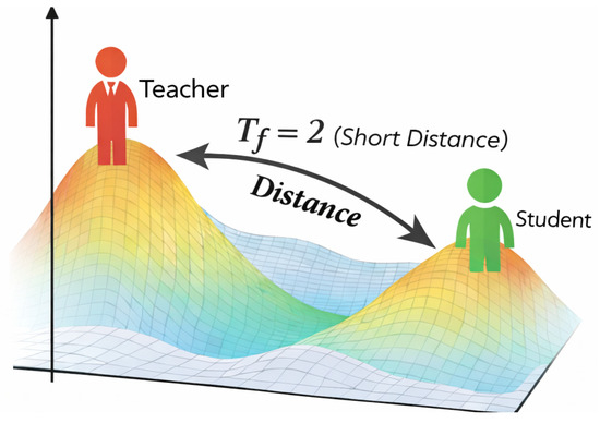
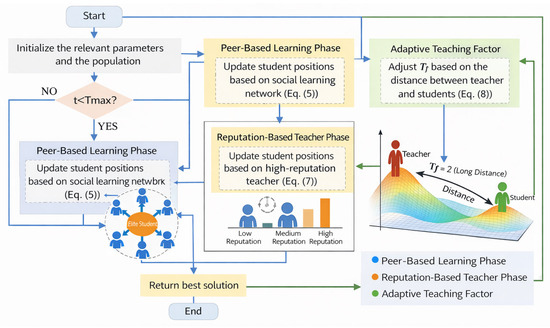
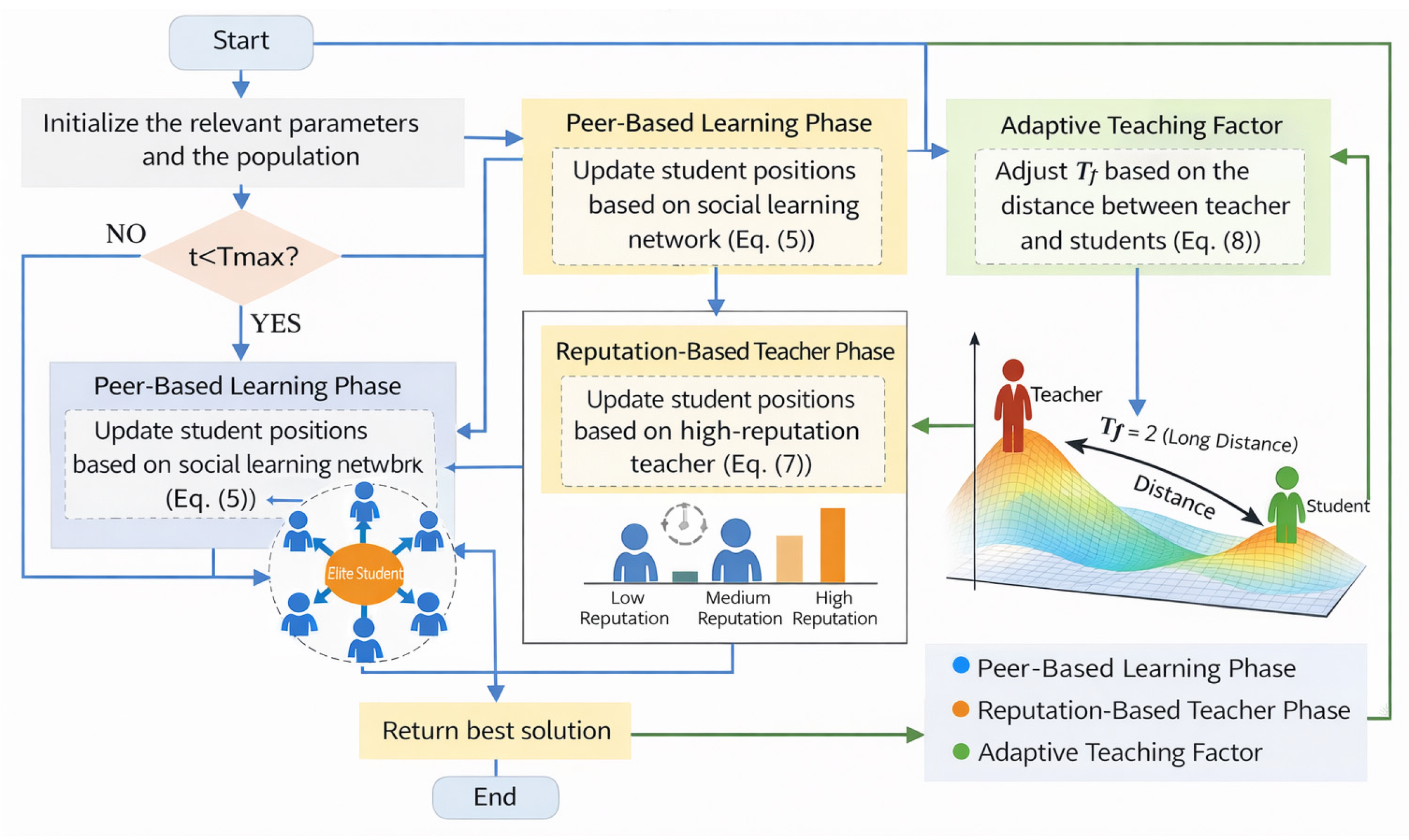
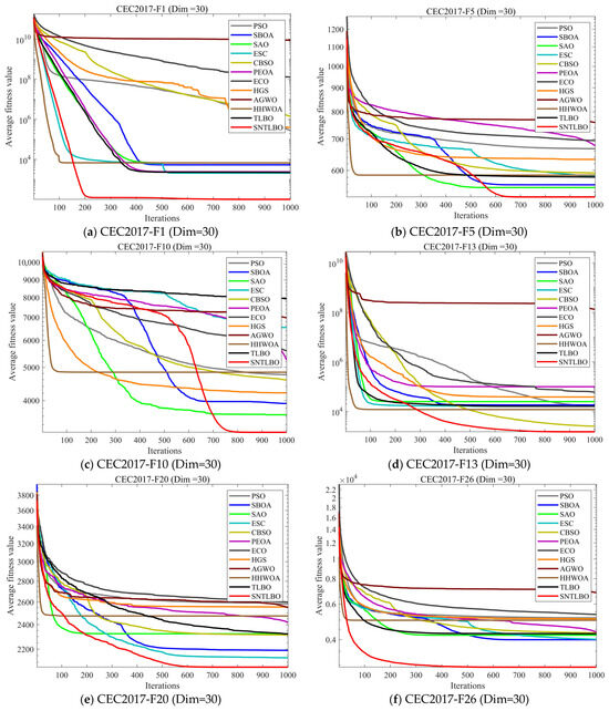
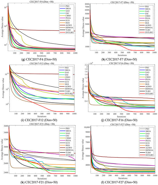
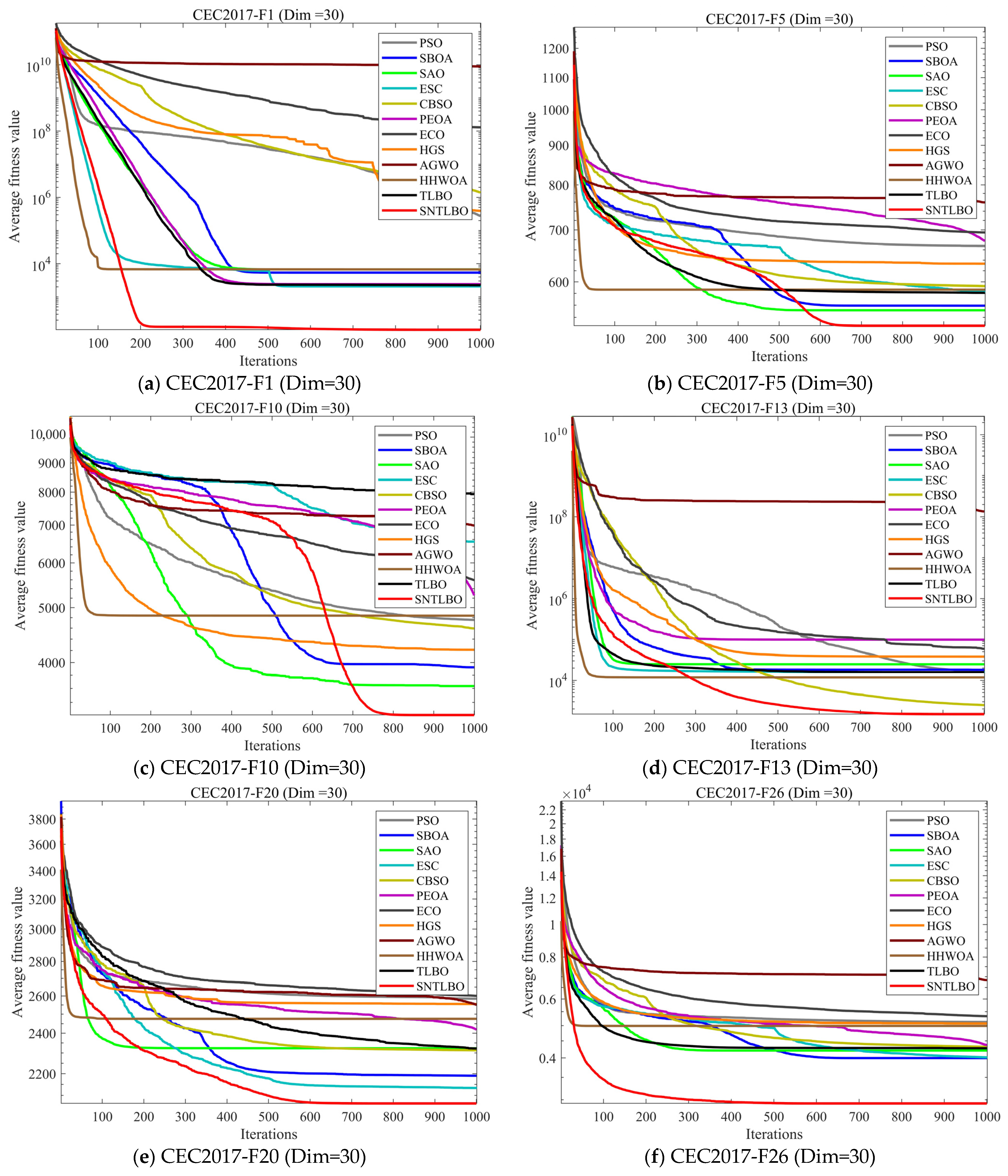
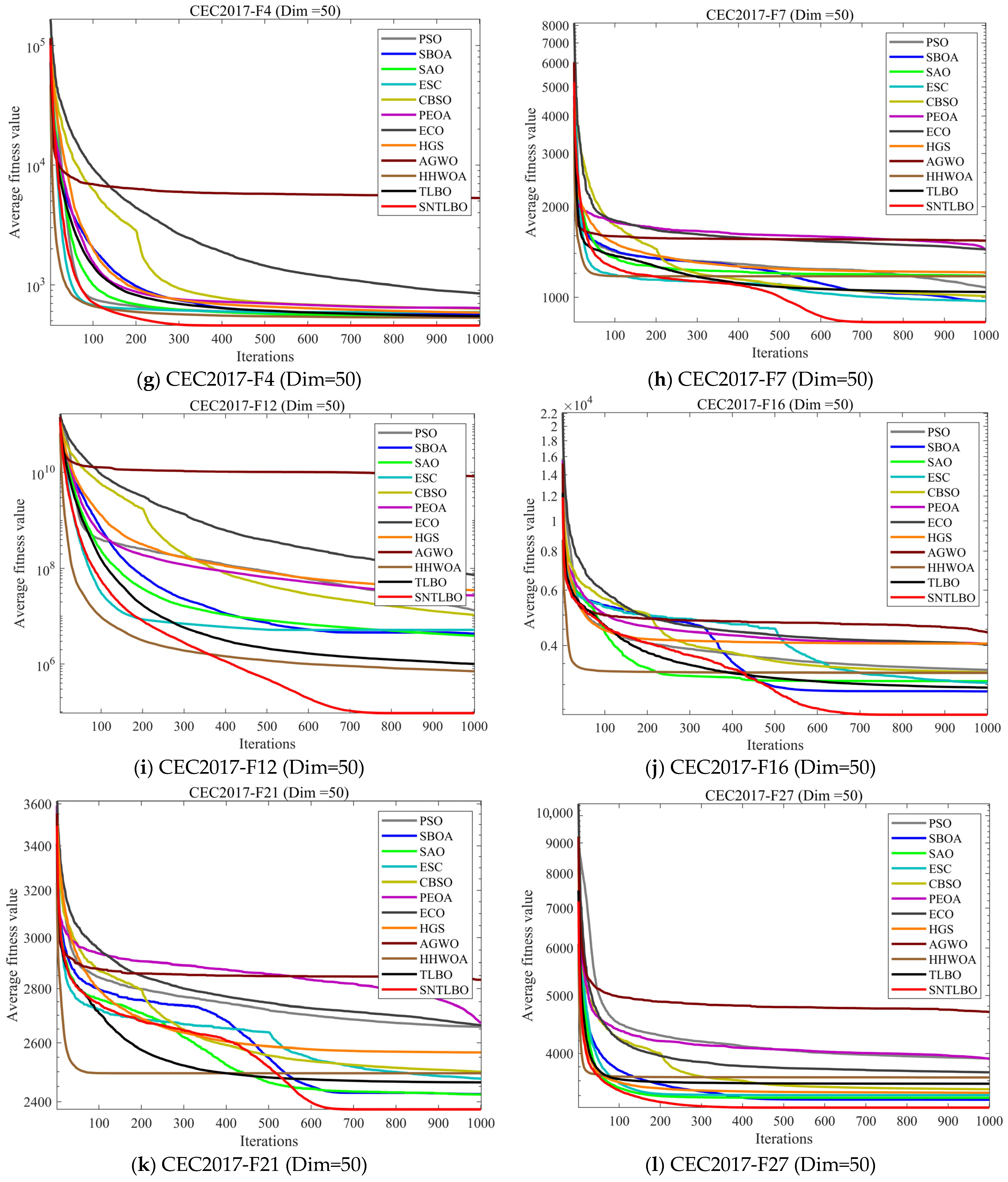
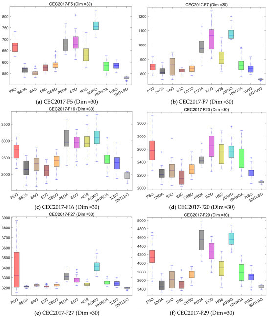
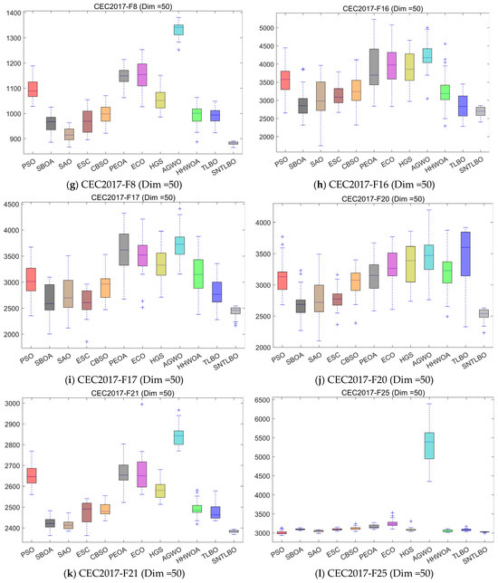
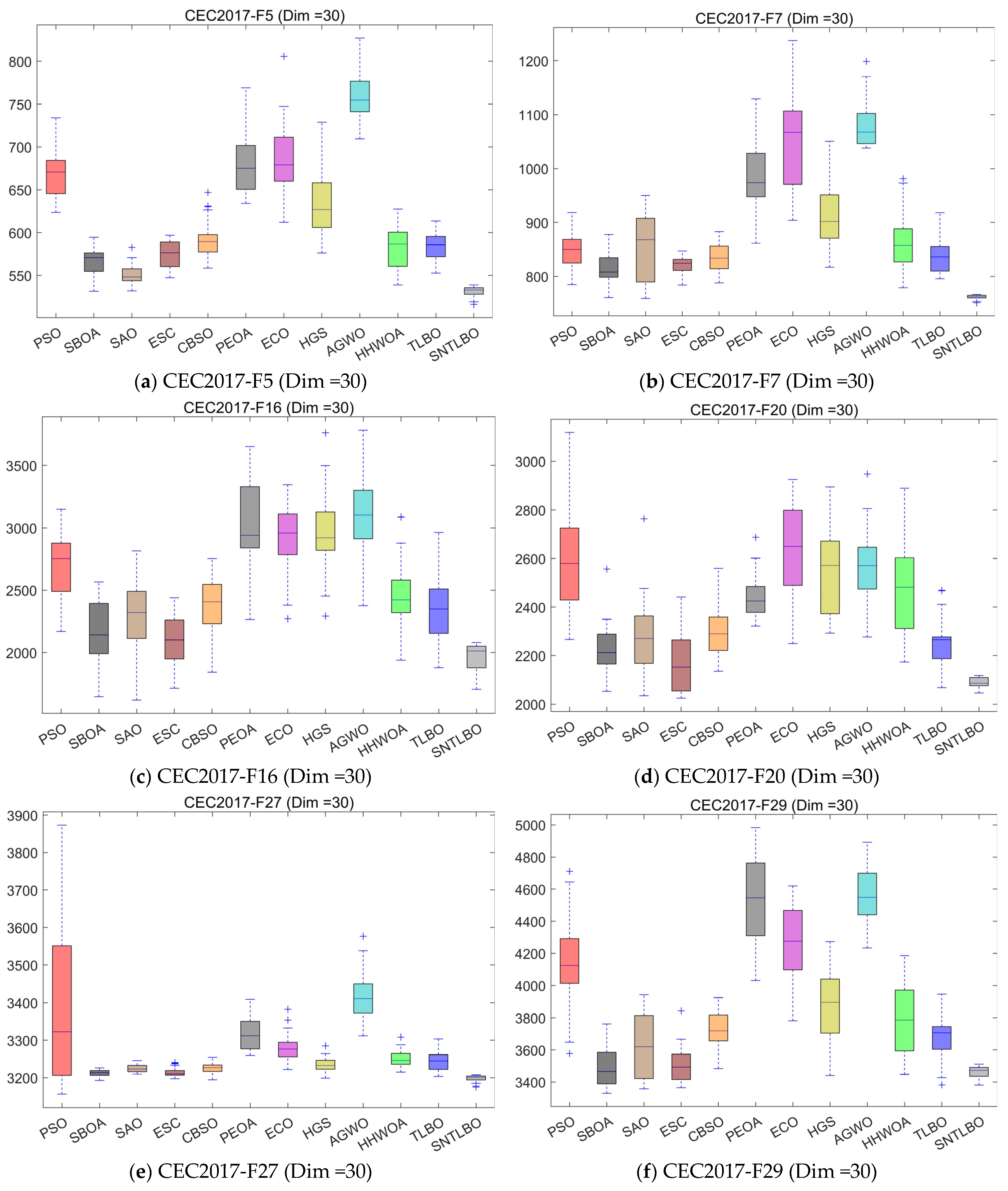
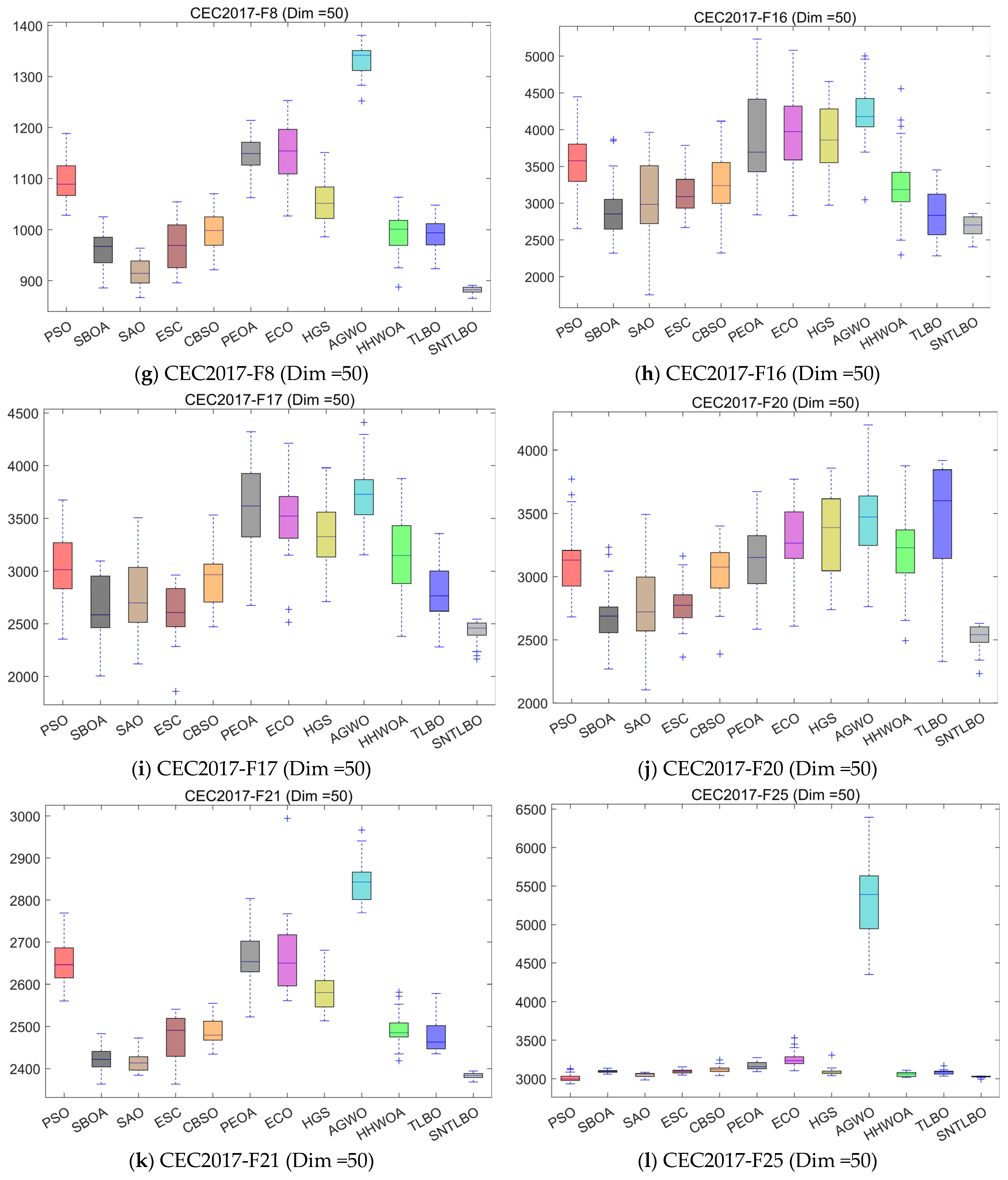
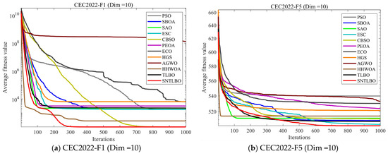
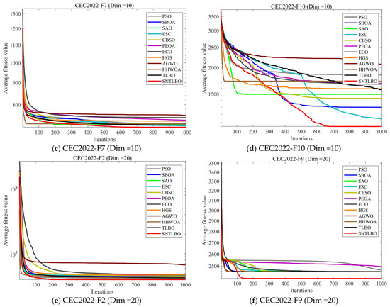
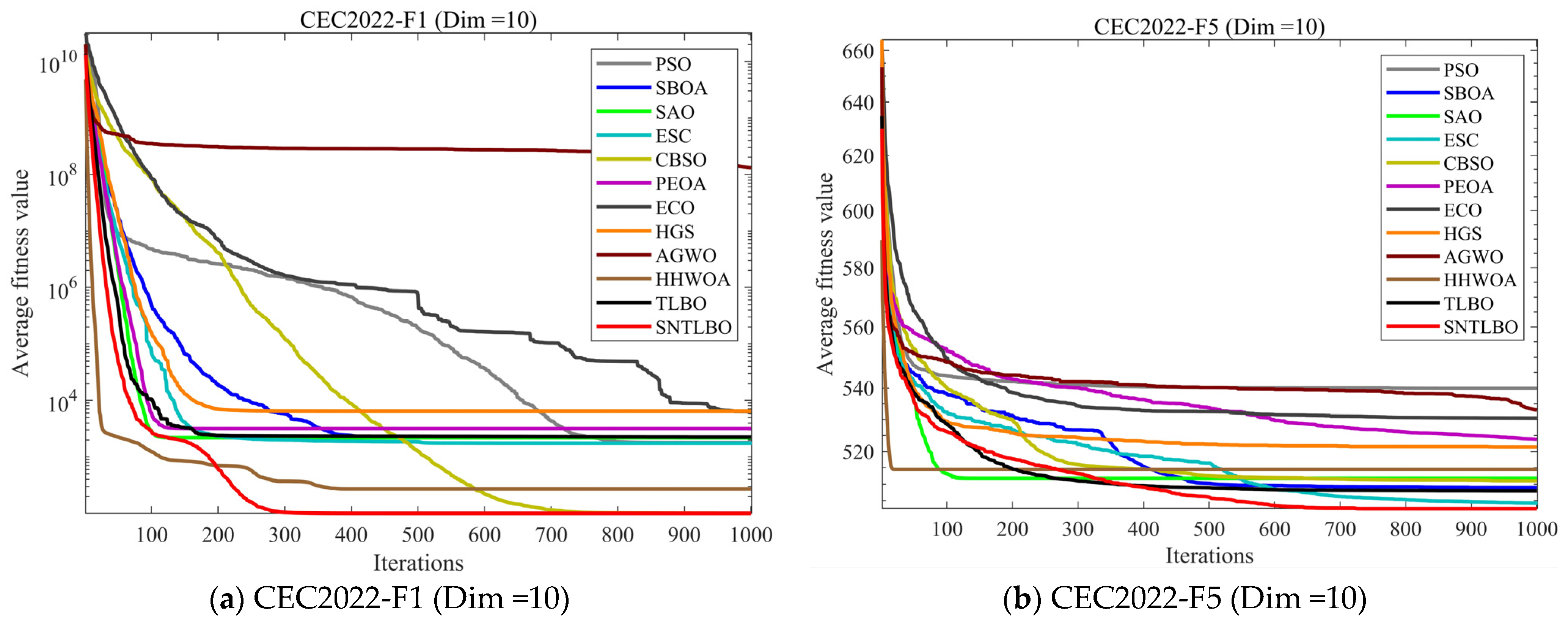
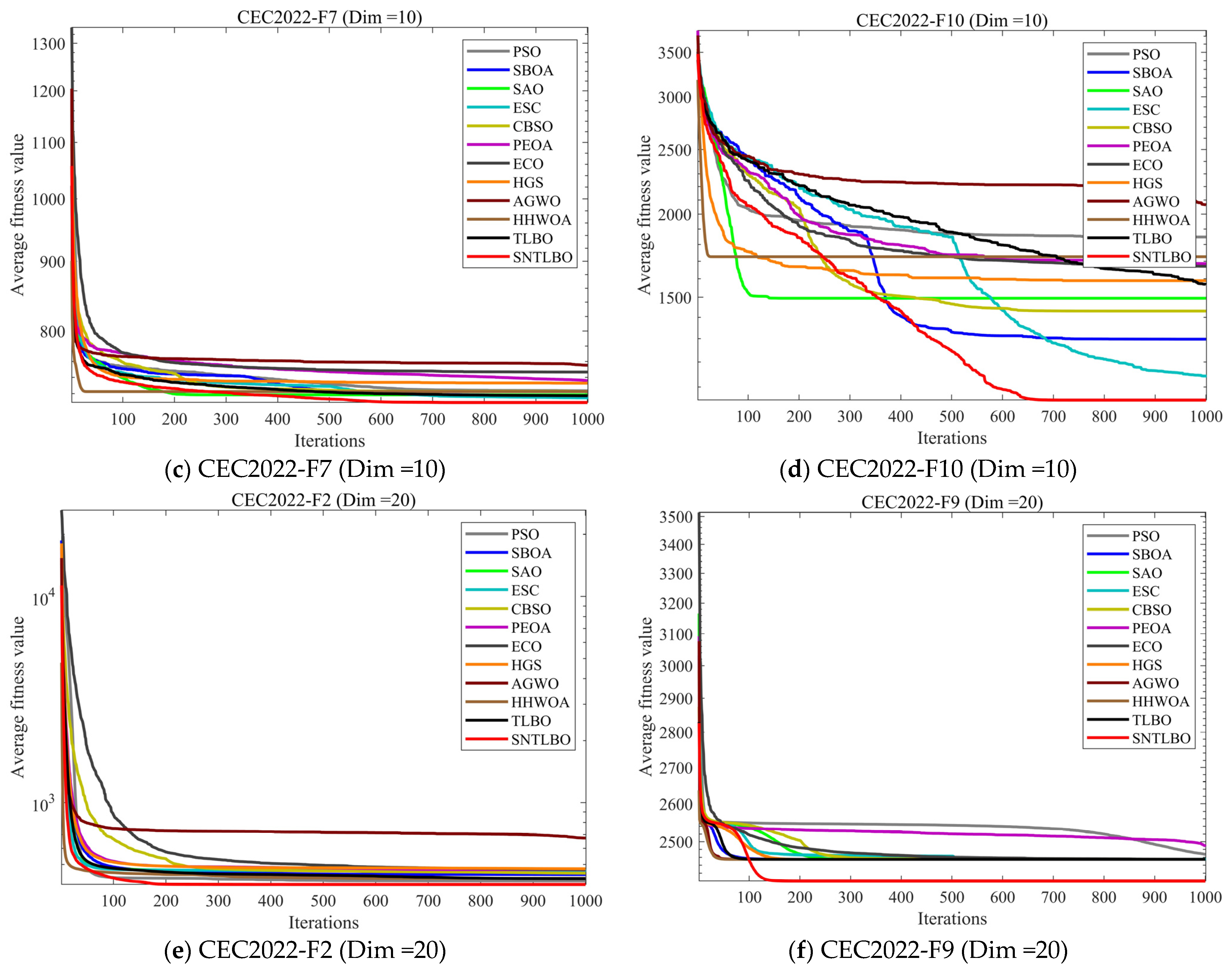
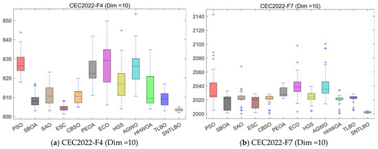
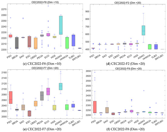
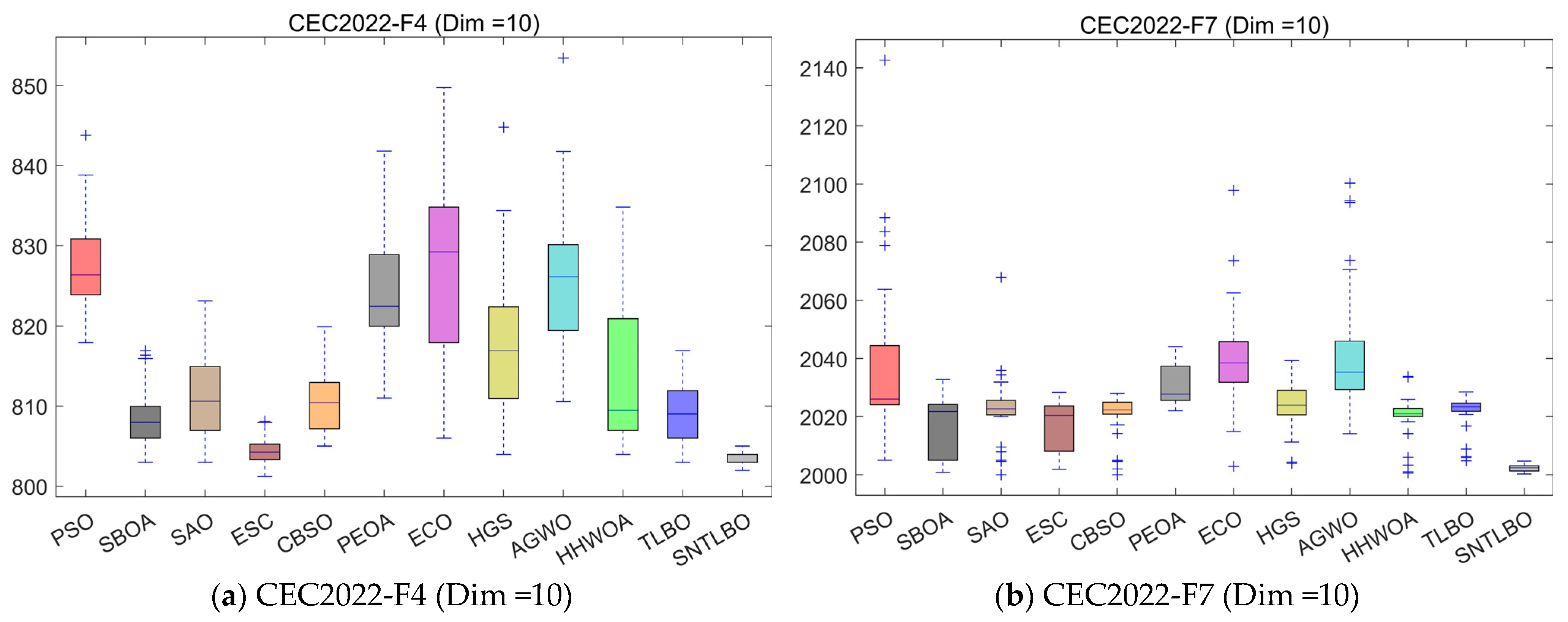
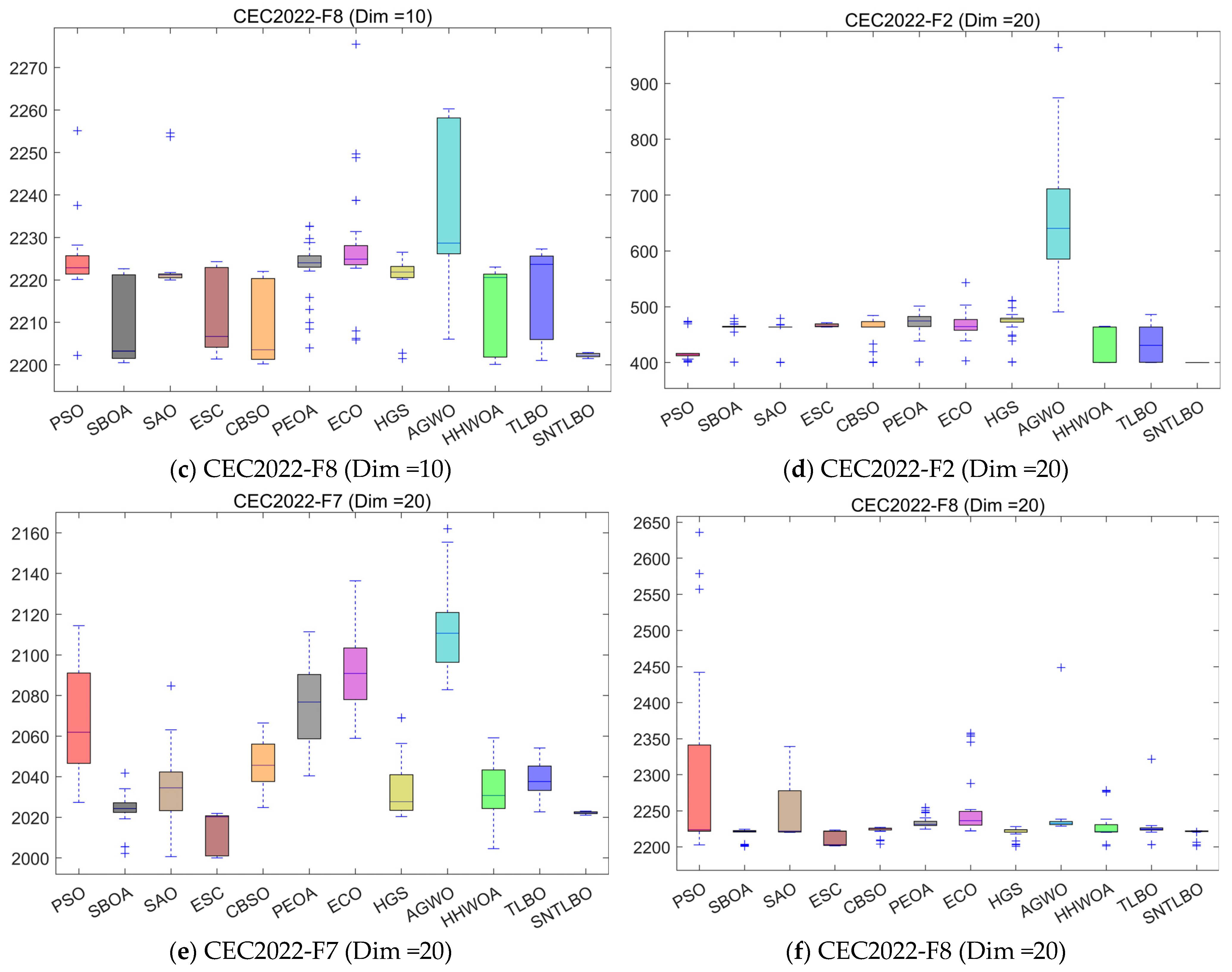
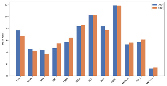
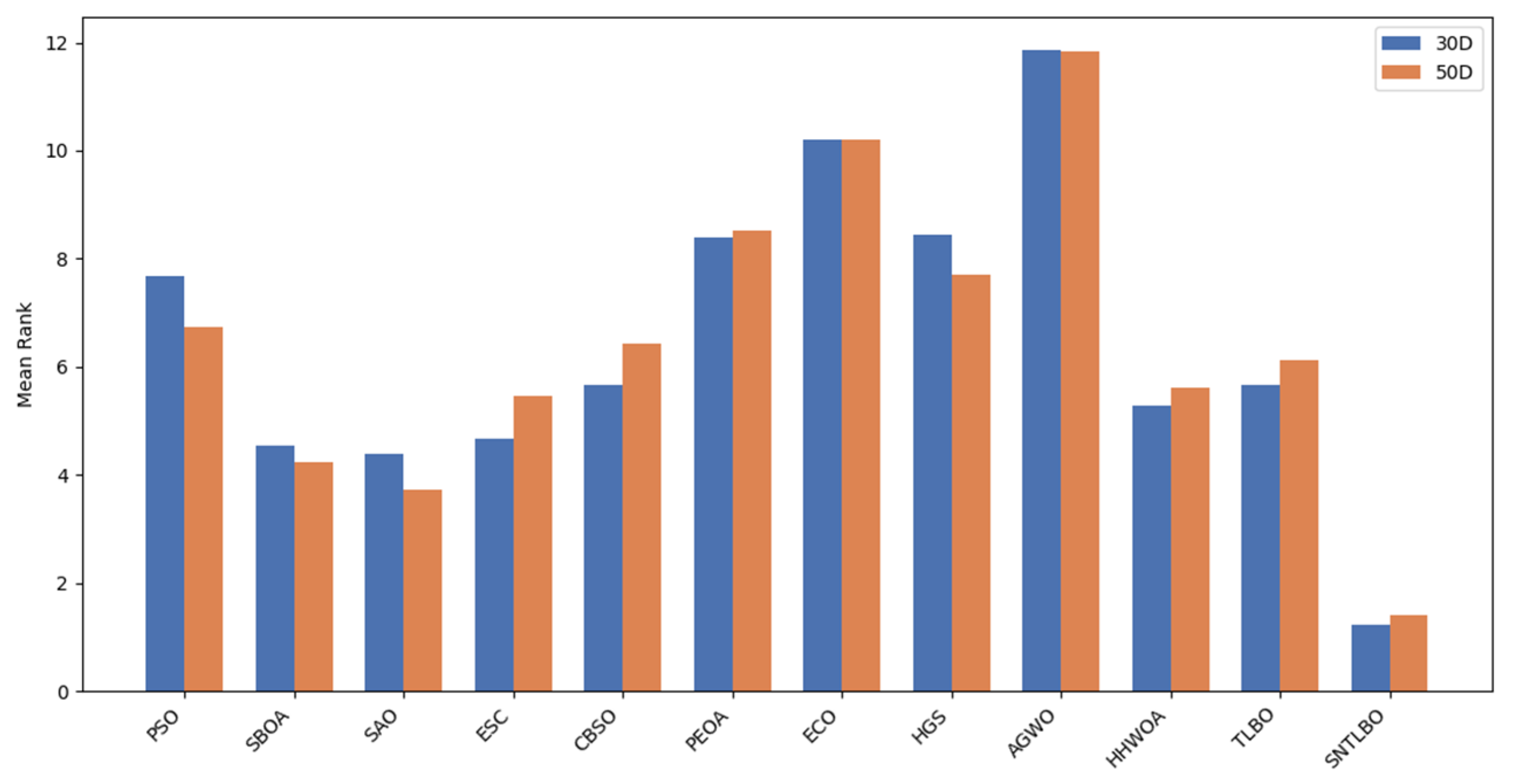
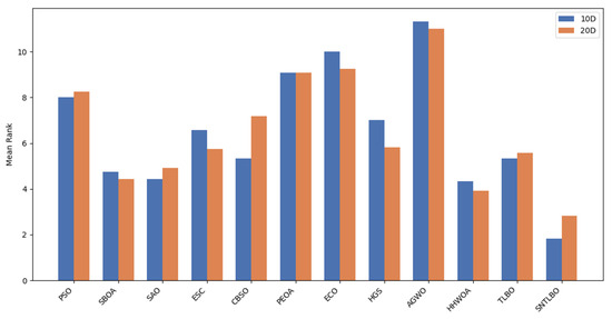
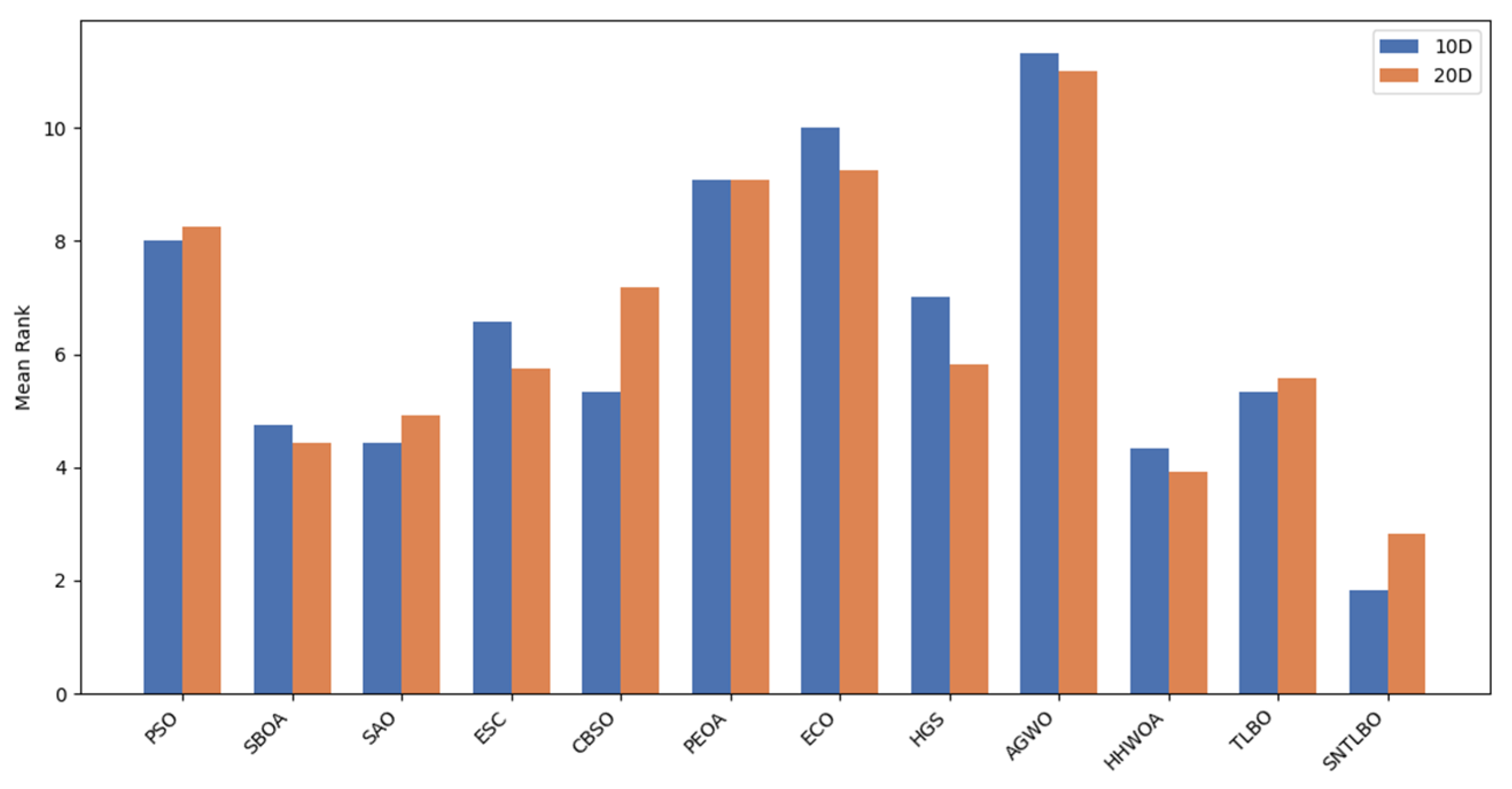
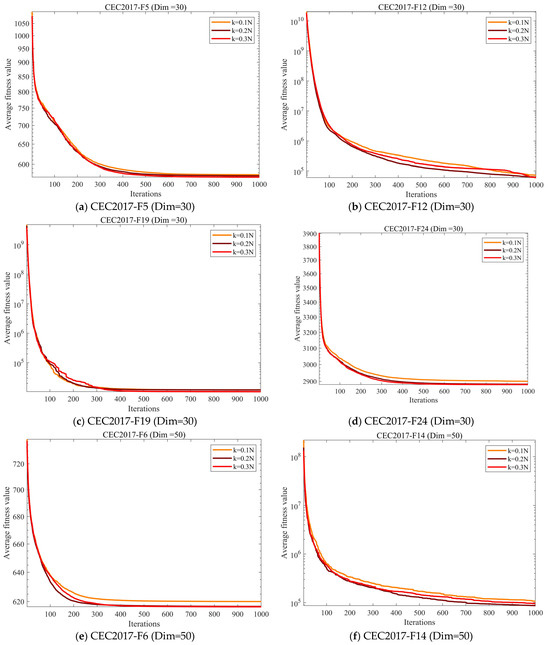
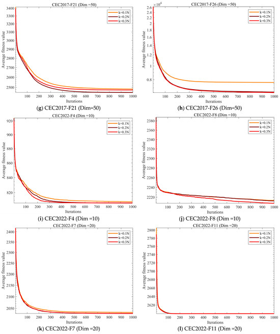
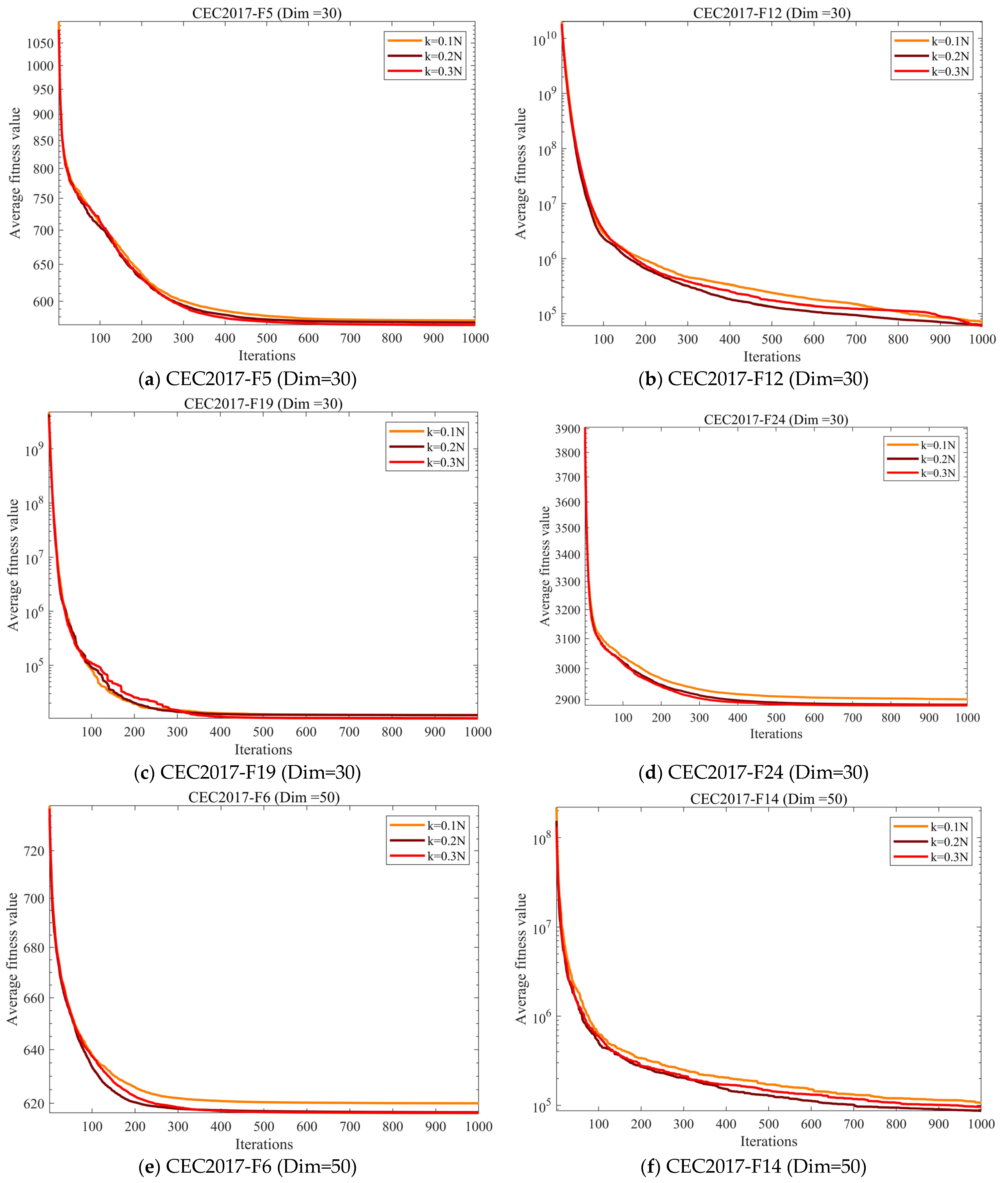
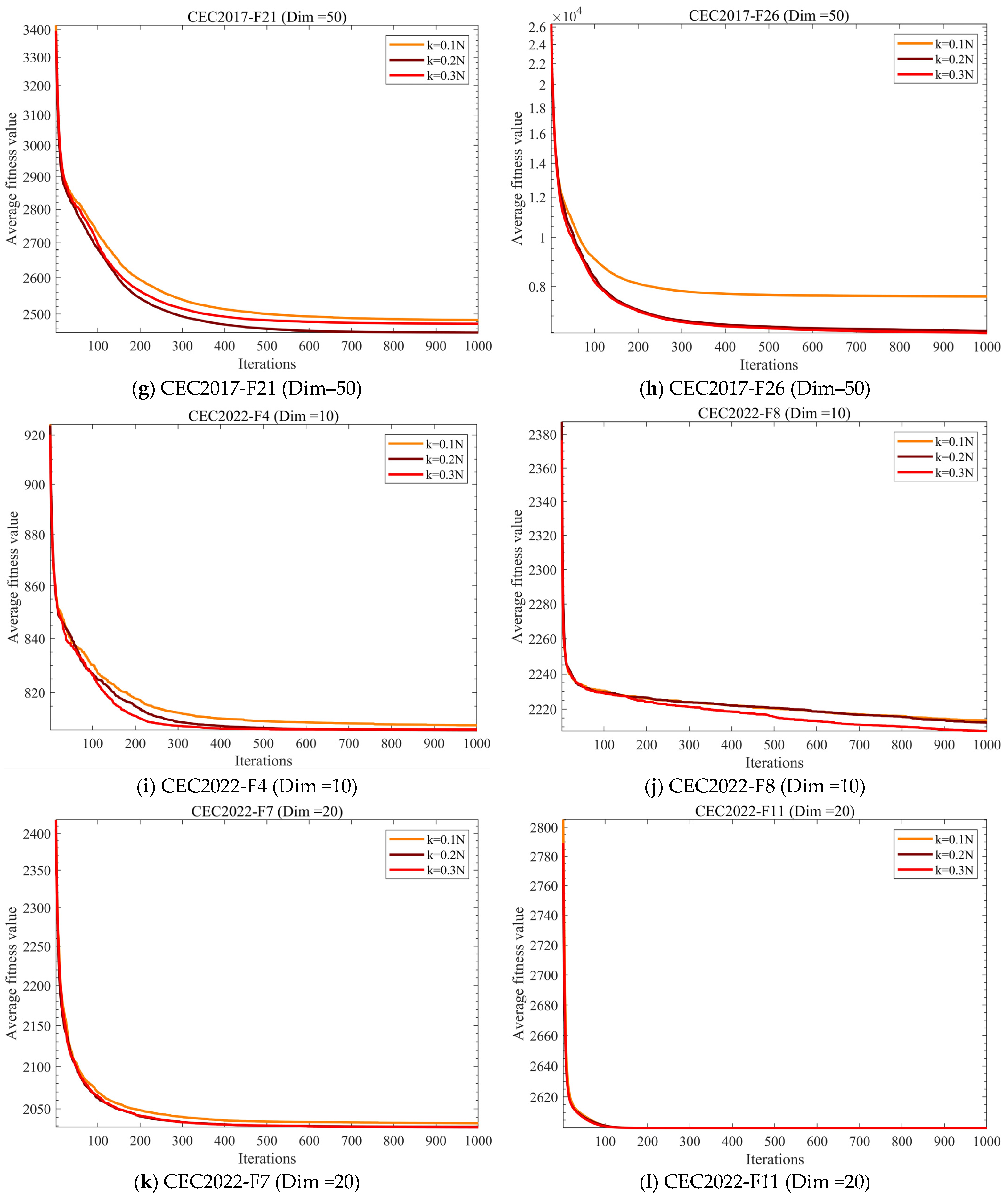
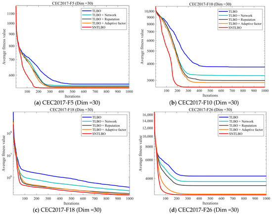
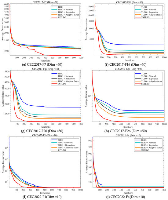
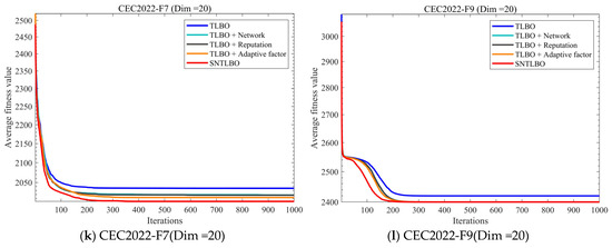
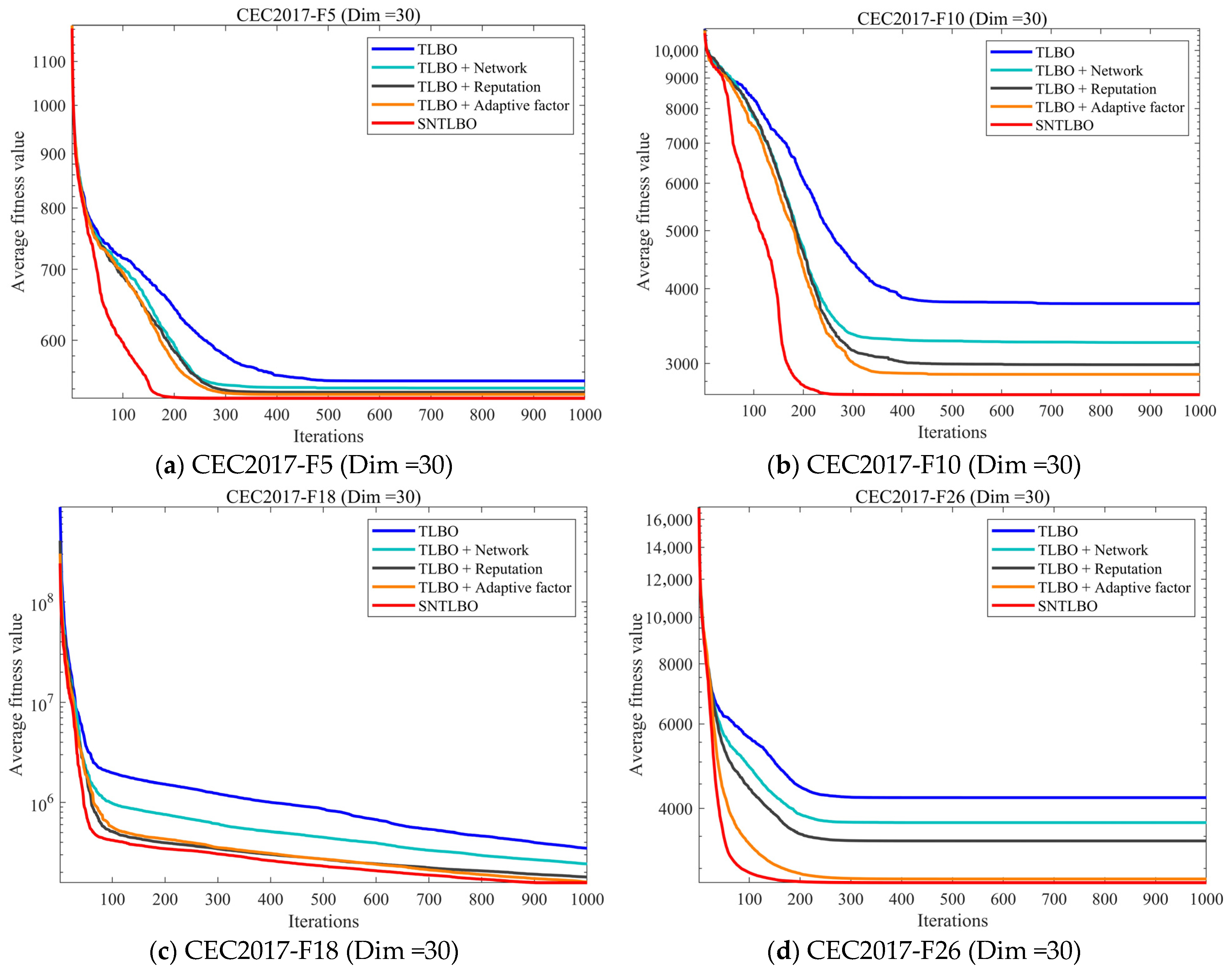
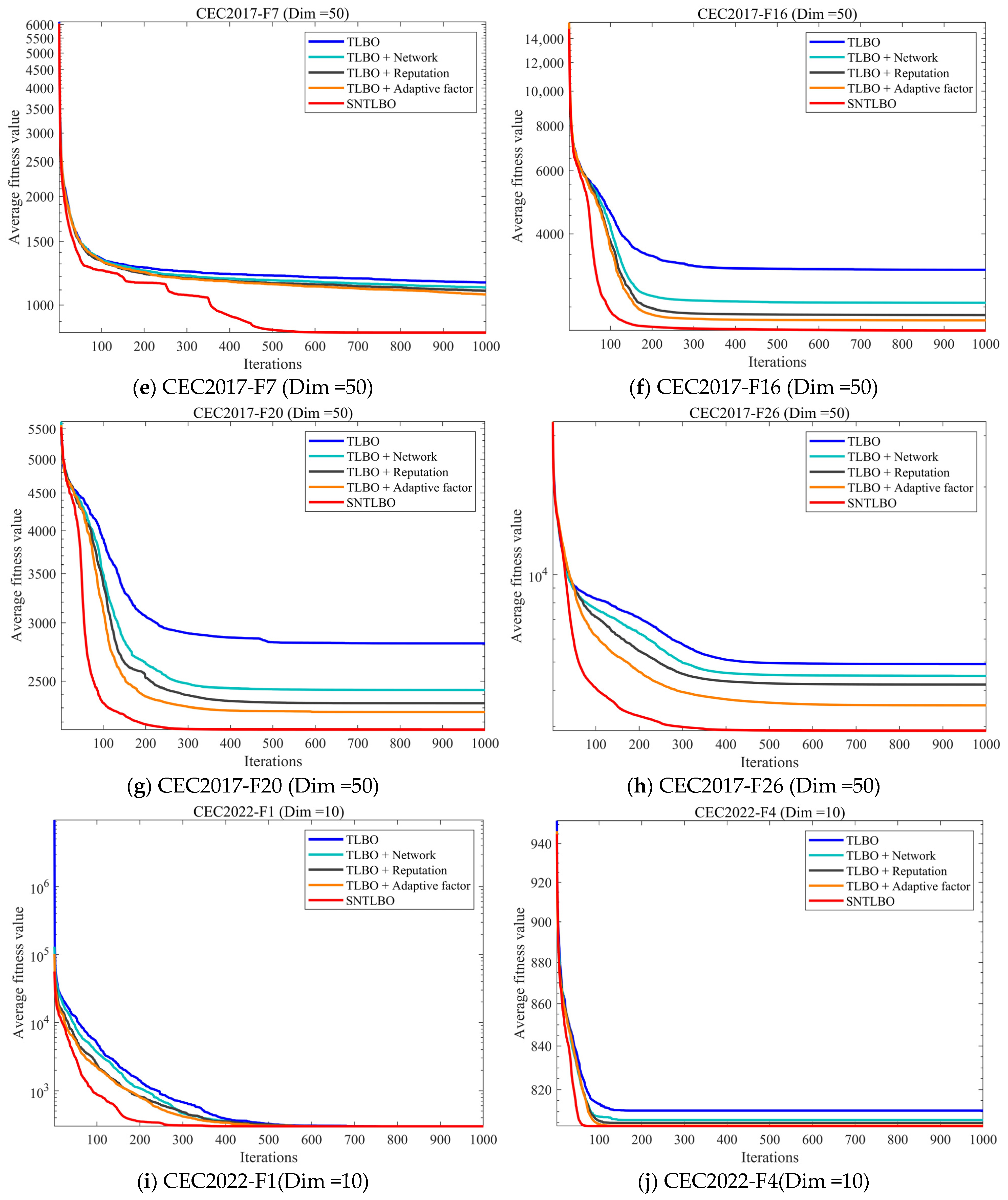
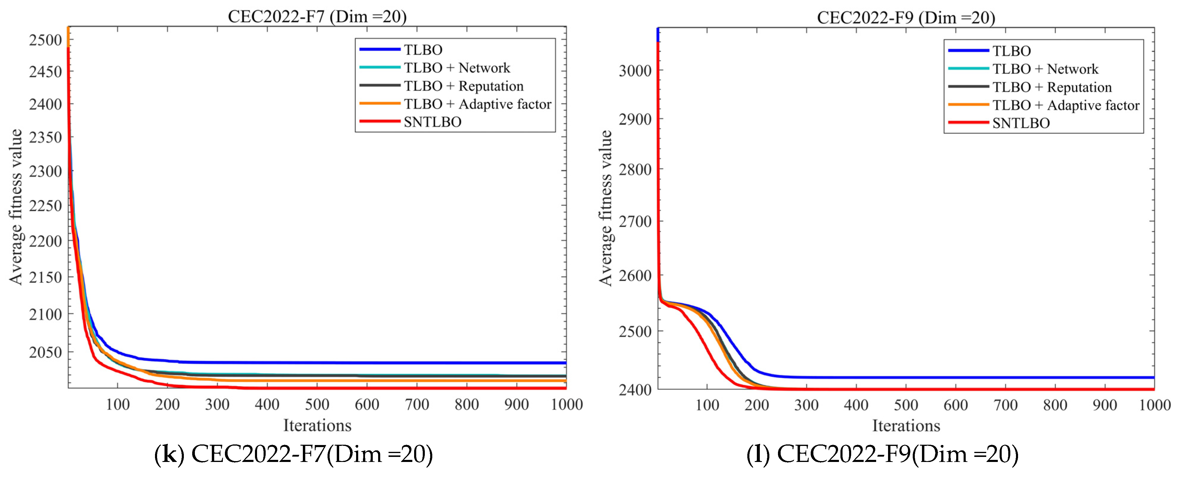
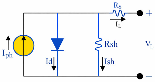
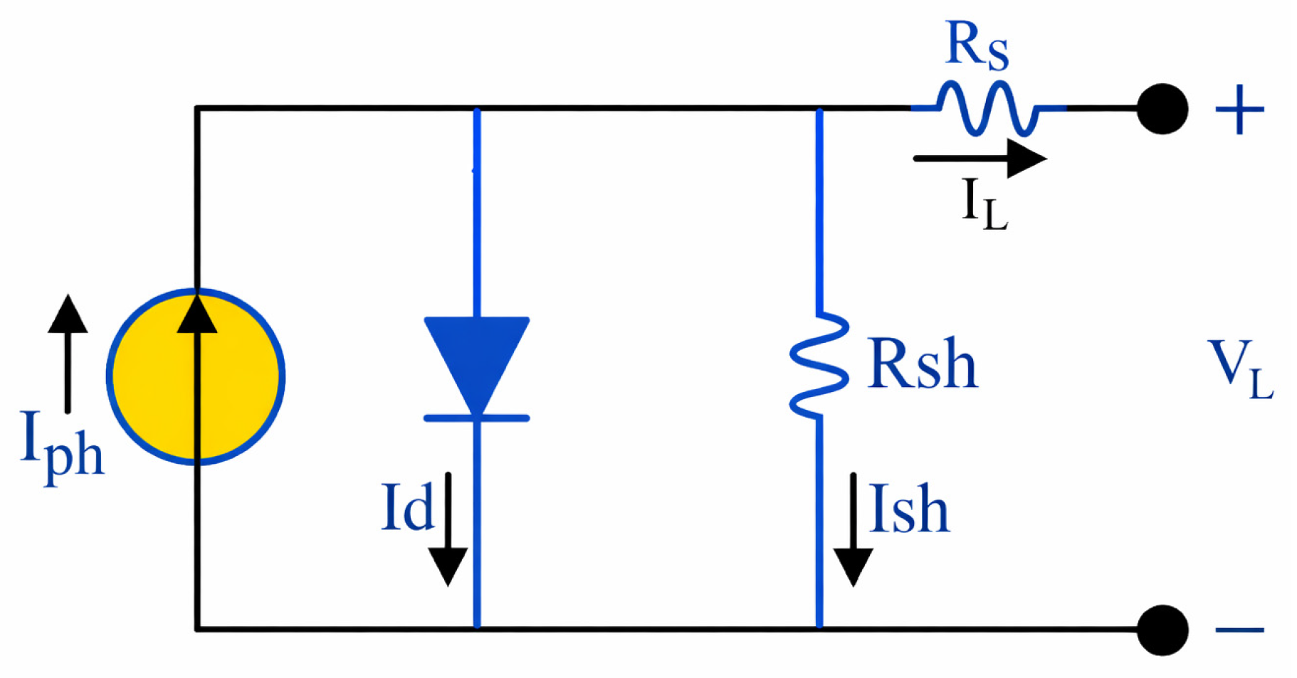
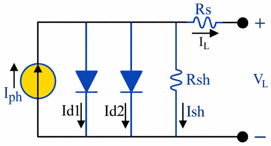
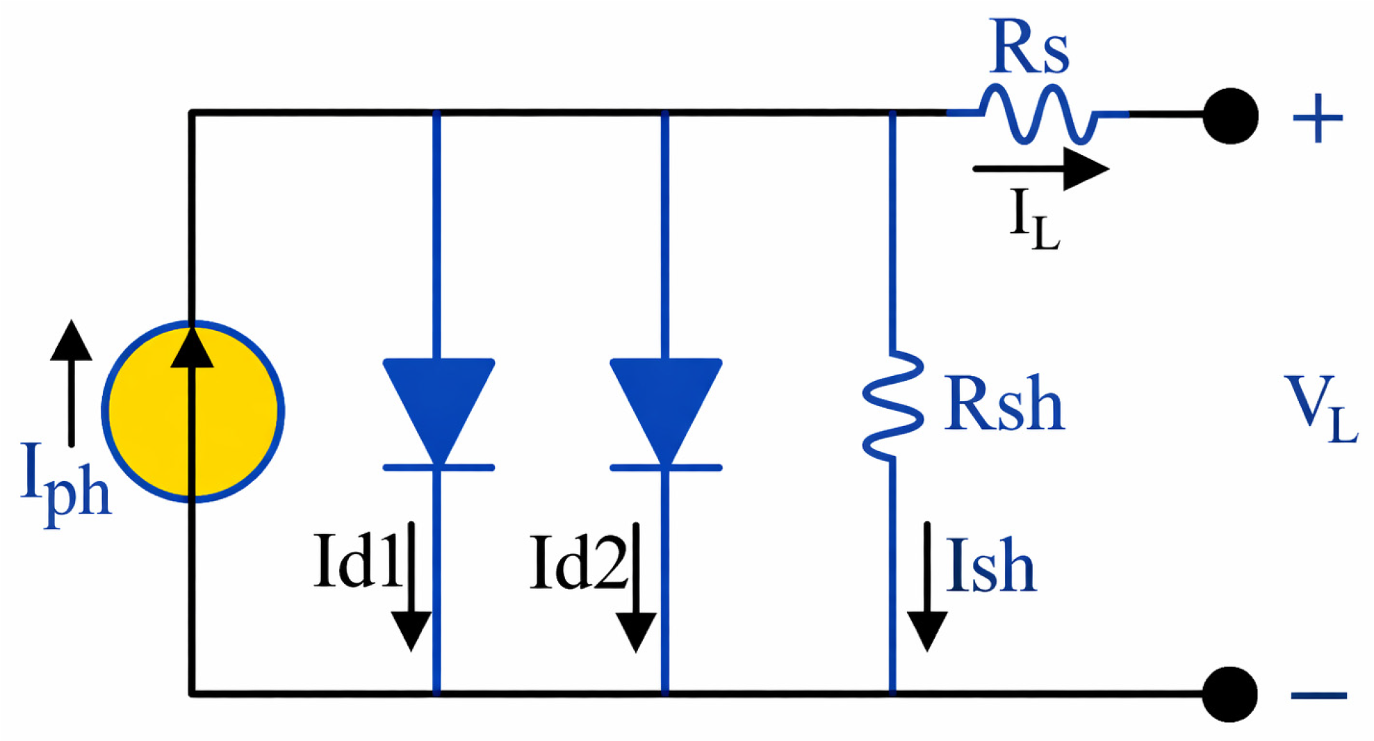
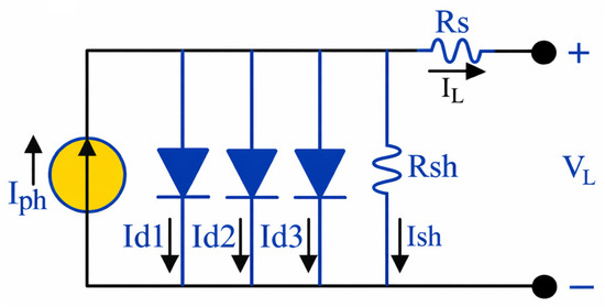
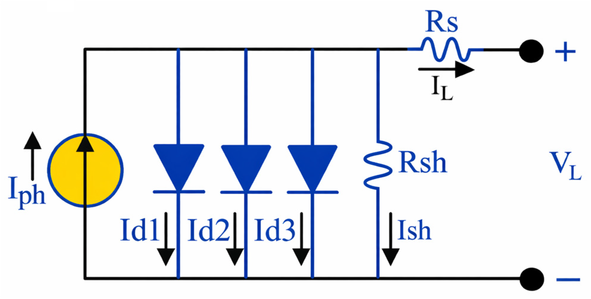
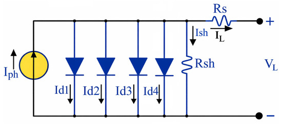
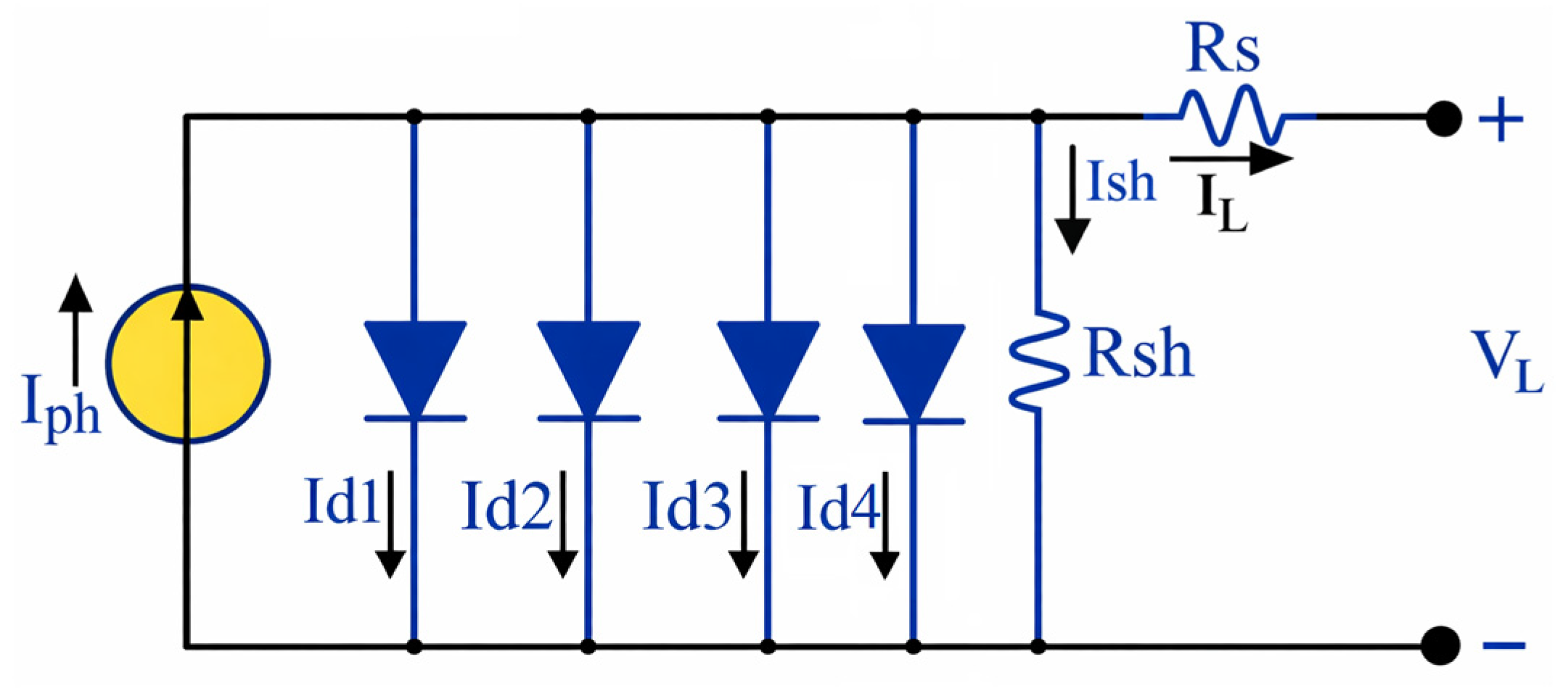
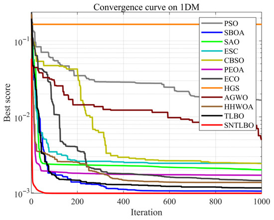
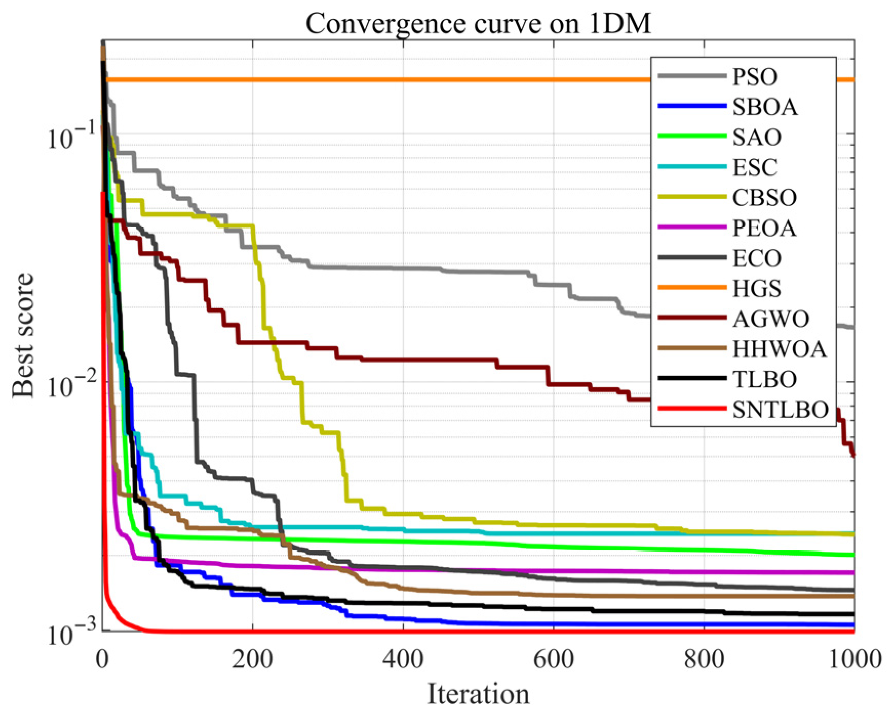
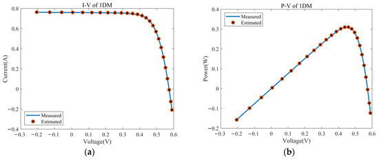
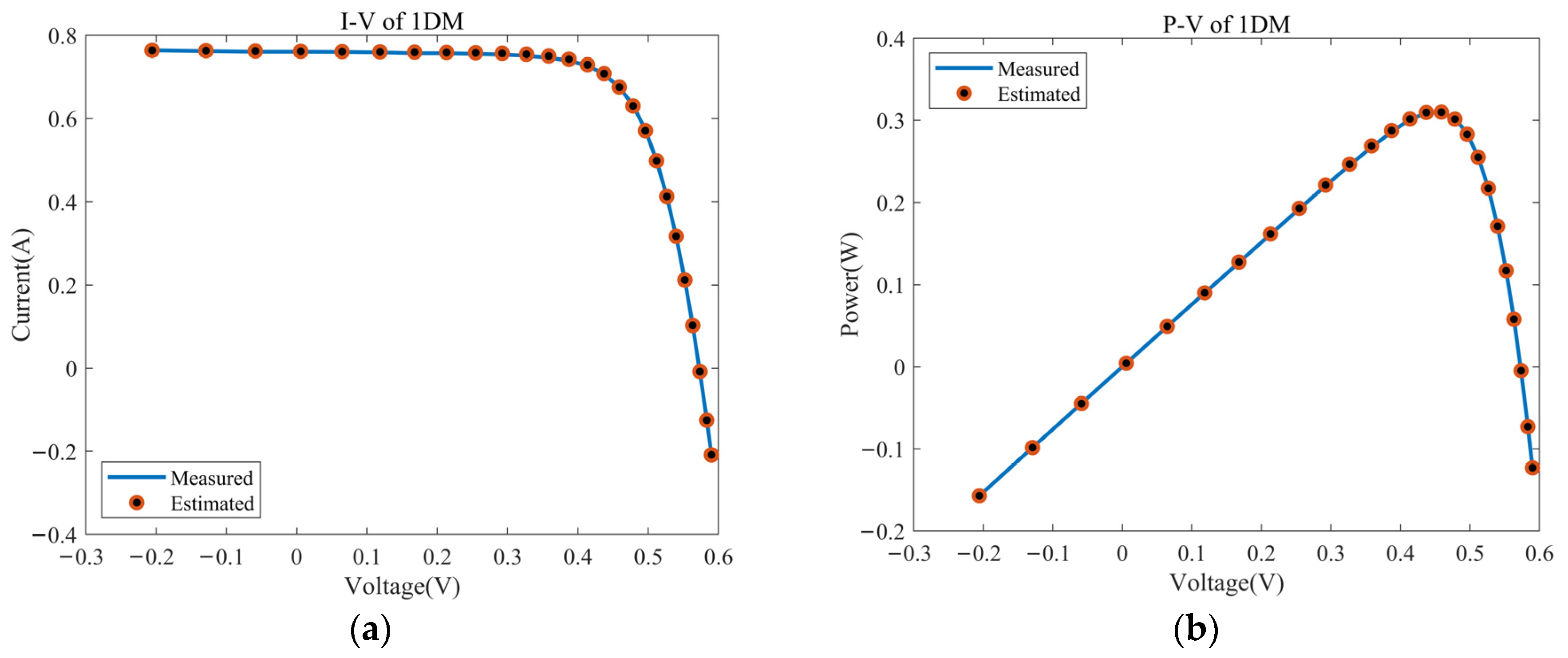
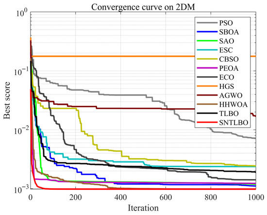
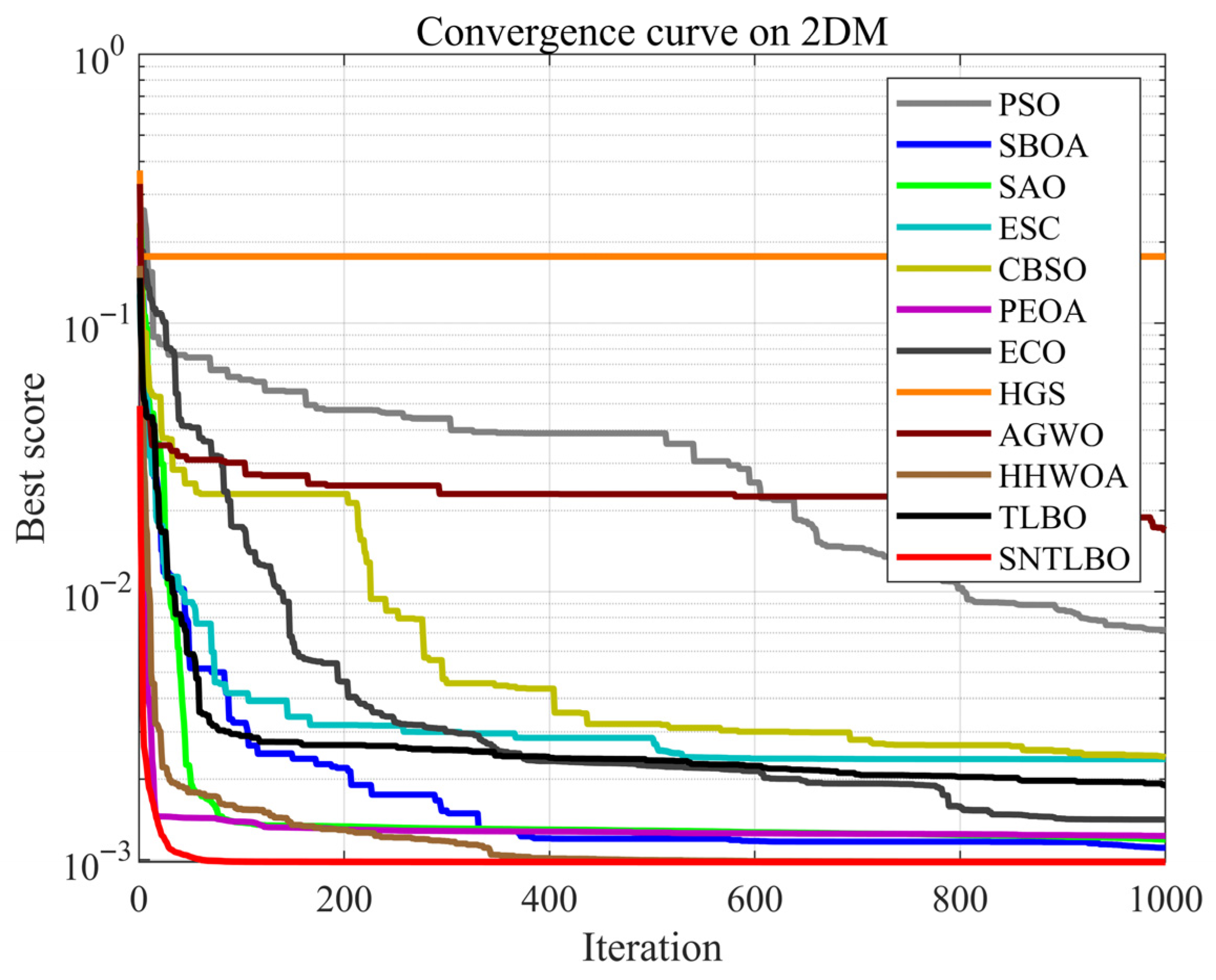
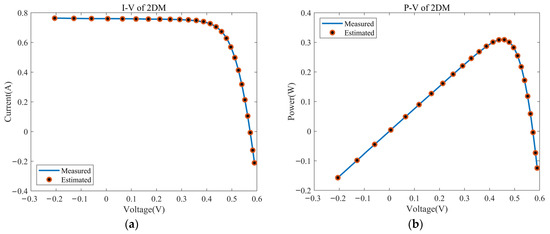
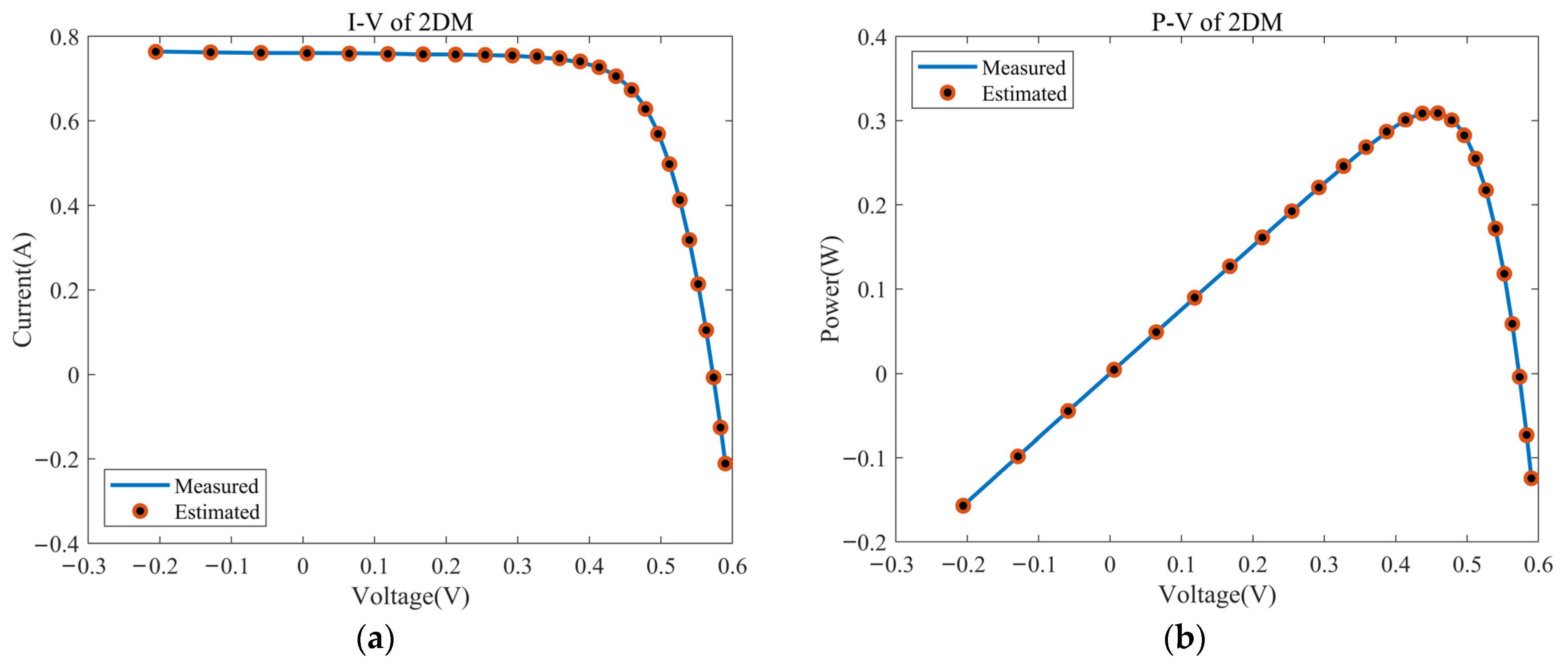
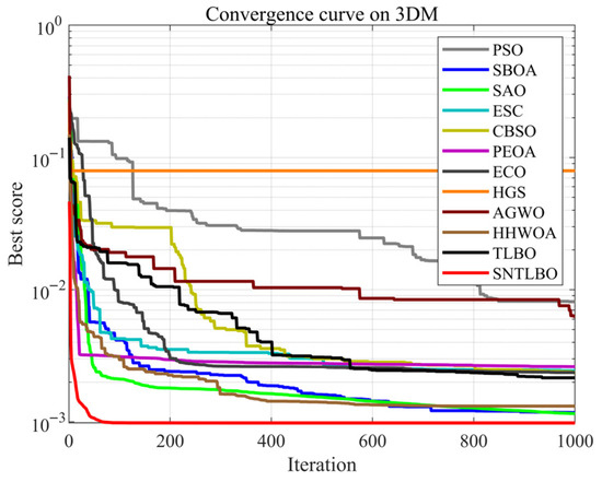
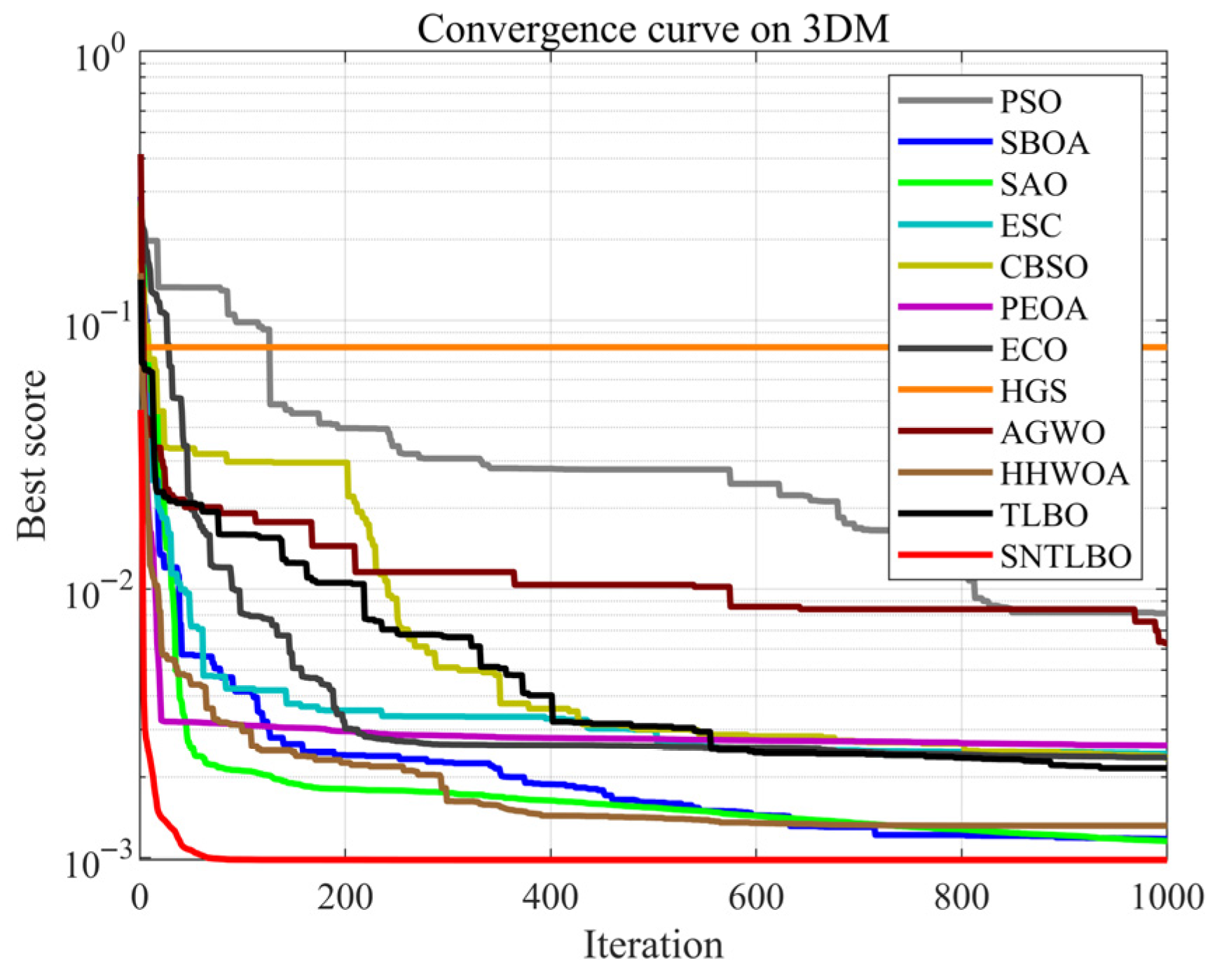
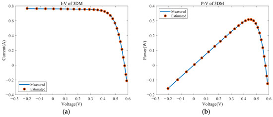
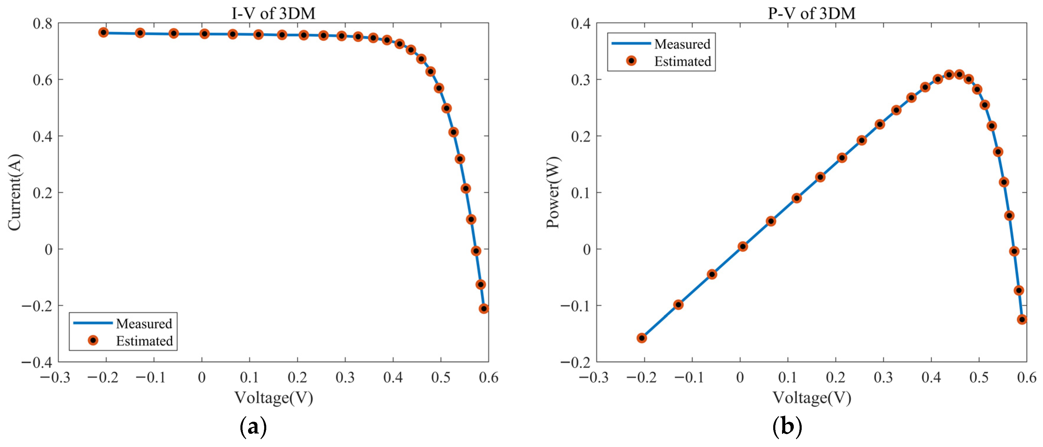
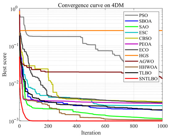
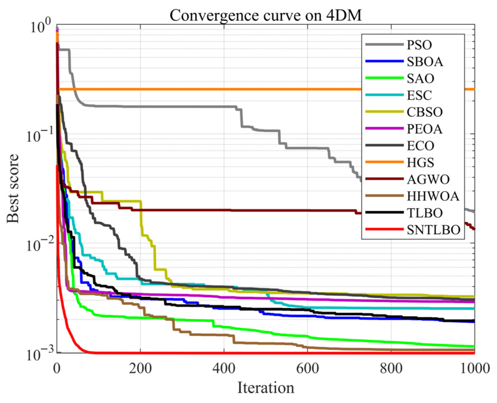
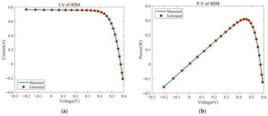
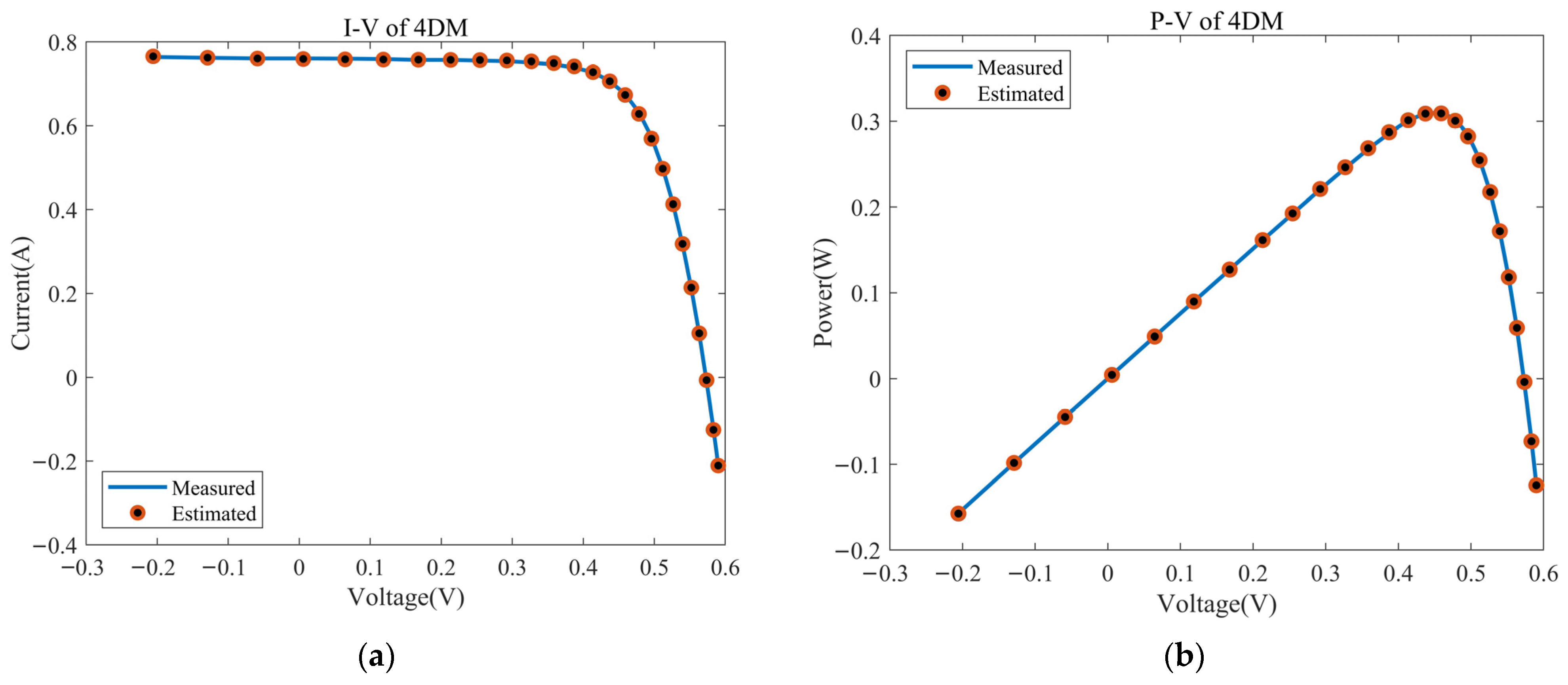
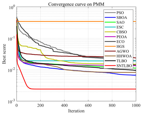
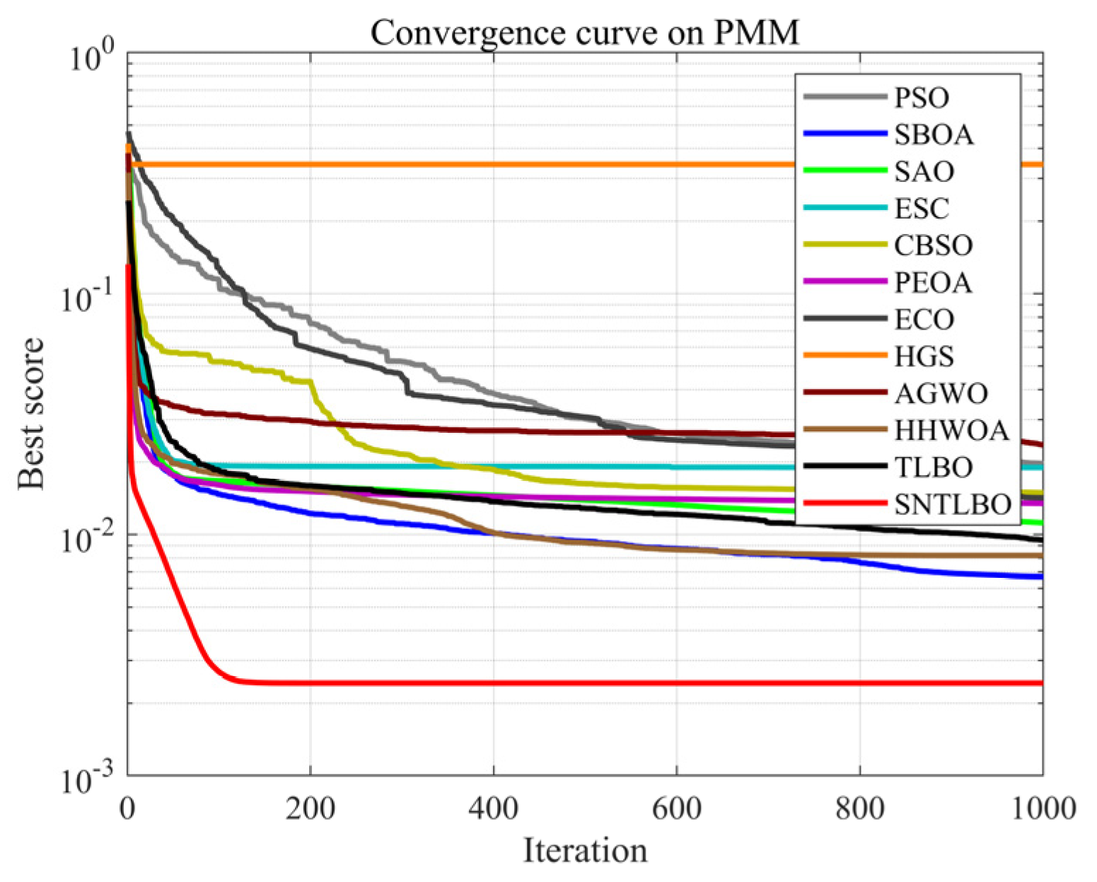
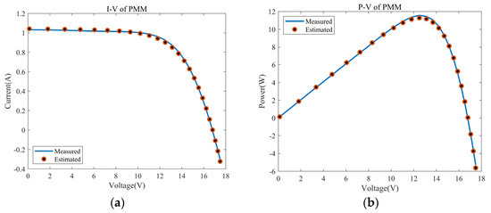
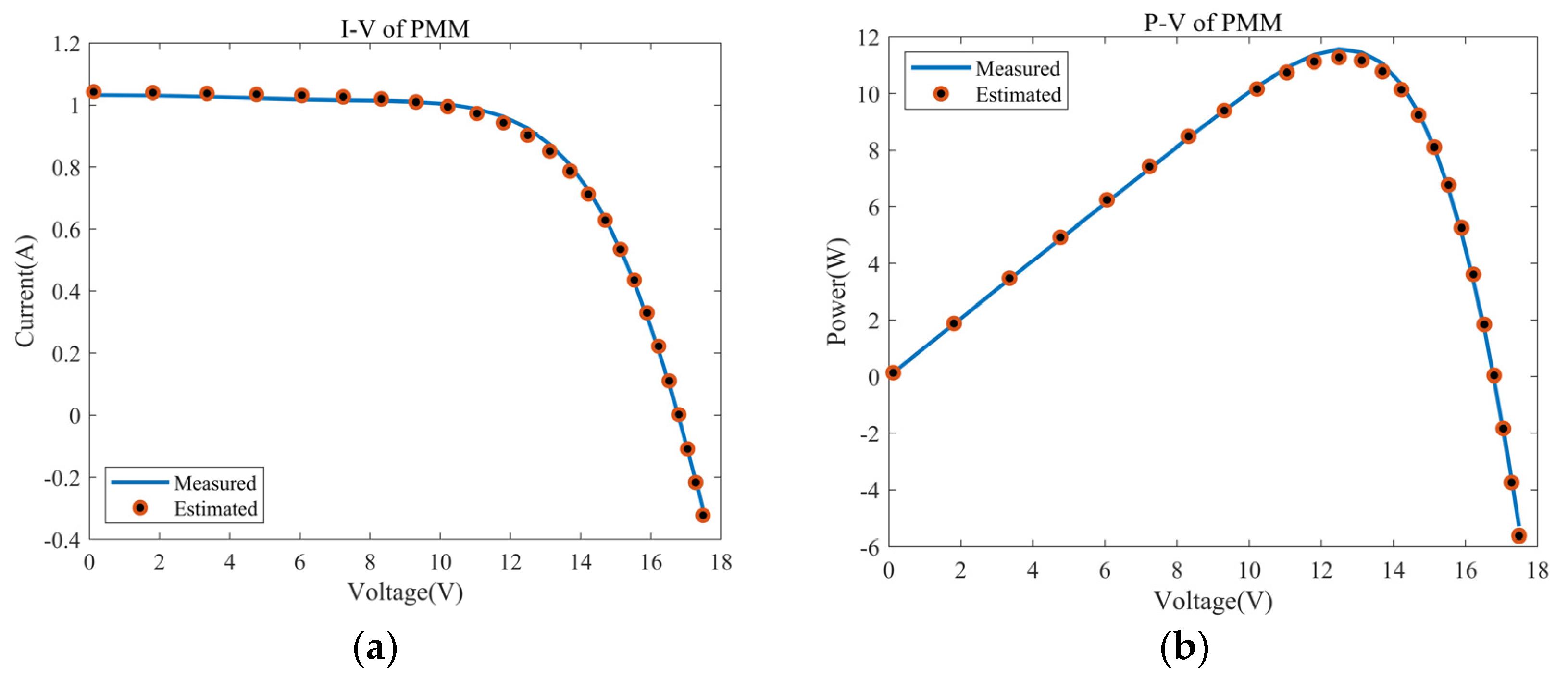

Disclaimer/Publisher’s Note: The statements, opinions and data contained in all publications are solely those of the individual author(s) and contributor(s) and not of MDPI and/or the editor(s). MDPI and/or the editor(s) disclaim responsibility for any injury to people or property resulting from any ideas, methods, instructions or products referred to in the content. |
© 2026 by the authors. Licensee MDPI, Basel, Switzerland. This article is an open access article distributed under the terms and conditions of the Creative Commons Attribution (CC BY) license.