Enhancing Active Distribution Network Resilience with V2G-Powered Pre- and Post-Disaster Coordination

Abstract

With the increasing penetration of distributed energy resources, distribution networks face elevated risks of power disruptions, which call for rapid and flexible emergency response mechanisms. There are not enough traditional emergency generator vehicles, and they are not highly adaptable when it comes to operations, which makes it hard to meet changing dispatching needs. Electric vehicles (EVs), on the other hand, can be used as distributed emergency resources that can be dispatched through vehicle-to-grid (V2G) interaction. Electric vehicle charging stations (EVCSs), on the other hand, are integrated energy storage units that use existing charging infrastructure to provide on-site grid support. To address this gap, this study proposes a comprehensive V2G-powered pre- and post-disaster coordination framework for enhancing distribution network resilience, with three core novelties: first, a refined individual EV model considering dual power and energy constraints is developed, and the Minkowski summation method is applied to accurately quantify the real-time aggregate regulation potential of EVCSs for the first time; second, a two-stage robust optimization model is formulated for pre-event strategic planning, which jointly optimizes EVCS participant selection and distribution network topology to address photo-voltaic (PV) power generation uncertainties; third, a multi-source collaborative dynamic scheduling model is constructed for post-disaster recovery, which explicitly incorporates the spatiotemporal dynamics of EVs and coordinates EVCSs, gas turbine generators (GTGs) and other resources for the first time. We carried out simulations on a modified IEEE 33-bus system with a 10 h extreme fault scenario. The results show that the proposed strategy raises the average critical load recovery ratio to 97.7% (2% higher than traditional deterministic optimization), lowers the total load shedding power by 0.2 MW and the load reduction cost by 19,797.63 CNY, and gives a net V2G power output of 3.42 MW (86.9% higher than the comparison strategy). The proposed V2G-enabled coordinated pre- and post-disaster fault recovery strategy significantly improves the resilience of distribution networks compared to traditional methods. This makes it easier and faster to recover from extreme disaster scenarios, with the overall load recovery rate reaching 91.8% and the critical load restoration rate staying above 85% throughout the recovery process.

1. Introduction

Because of the widespread use of distributed energy resources like photovoltaic (PV) and wind power, as well as different types of energy storage systems, the modern distribution network is going through significant modifications. These changes make energy architecture more beneficial to the ecosystem, but they also make systems harder to use and more likely to break down [1]. These resources have output that can’t be predicted, are spread out over a large area, and do not interact well with traditional grid frameworks. This means that the system is more likely to fail during severe weather or physical attacks, which can cause frequent large-scale outages that put the power supply at risk [2]. But this tough situation also gives us new opportunities. By taking a close look at grid-connected electric vehicles (EVs), one will see that they don’t just use electricity; they can also be used as a type of distributed energy storage that can be used at different times and places. It is possible to actively manage and combine their charge and discharge behaviors during grid stress or faults by using advanced information and communication technologies and coordinated control strategies. This turns this massive, spread-out resource from a possible source of trouble into a valuable, adaptable asset that helps with emergency recovery and makes the grid more resilient [3,4]. So, large-scale vehicle-to-grid (V2G) interaction has two sides: it increases operational risks while also giving utilities a new way to actively improve system resilience through resource coordination and optimization [5].

To systematically comprehend how EVs can enhance the resilience of the grid, most research adheres to three primary steps: evaluating their potential, allocating resources for prevention prior to a disaster, and facilitating recovery post-disaster [6,7,8]. But traditional models have significant challenges when it comes to handling the unique behavioral uncertainties that come with EVs. In the potential evaluation phase, the majority of conventional methodologies utilize static parameter models or steady-state aggregation techniques based on historical statistical data [9,10]. These methods offer a fundamental framework for potential estimation; however, they frequently oversimplify the intricate and dynamic characteristics of user travel and charging behaviors by representing them as deterministic or static probabilistic distributions. These kinds of simplifications fail to take into account how different each user’s preferences and real-time grid-interactive signals are, which makes it hard to accurately describe how electric vehicles actually work. Because of this, these traditional methods are not very good at accurately measuring the active power and energy regulation limits of electric vehicle charging stations (EVCS). Second, classical methods primarily employ deterministic optimization or scenario-based stochastic planning in the pre-disaster resource allocation phase [11,12,13]. When things are uncertain, like when the PV output changes or the fault locations are unknown, deterministic methods have a hard time. Stochastic planning, on the other hand, depends a lot on making correct assumptions about probability distributions. When there is not a lot of historical data or when disaster scenarios are very unlikely, the plans that come out of them are often not very strong [14]. Finally, most current strategies for dynamic recovery after a disaster focus on traditional resources like generators (GTGs) and fixed energy storage systems. Scheduling models are either static or split [15,16]. The current scholarly literature on electric vehicles frequently employs an overly simplistic portrayal, predominantly conceptualizing EVs as stationary energy storage entities [17,18]. This conventional modeling paradigm fails to account for the intrinsic mobility of electric vehicles as spatially relocatable energy assets, which constitutes one of their most distinctive and operationally vital characteristics. By disregarding the dynamic spatial-temporal characteristics of EVs, such methodologies neglect to account for the intricate interdependencies between vehicle mobility behaviors and real-time grid interactions [19]. As a result, these simplified models cannot fully reflect the actual operational flexibility and regulatory potential of electric vehicles, which significantly restricts the accuracy, reliability, and practical applicability of the derived strategies for grid stability enhancement, optimal resource allocation, and efficient energy dispatch [20]. These issues underscore the necessity of establishing a framework for integrated modeling and optimization that interlinks these stages and comprehensively incorporates the spatiotemporal dynamics of EVs [21].

In the domain of adjustable potential assessment theory, Minkowski set operations have been acknowledged as the essential framework for delineating the feasible scheduling domain of aggregated resources. But most traditional applications only use static, offline estimates of every individual’s feasible region. For instance, they believe that all vehicles have the same limits on how much power they can charge and discharge, and that the state of charge trajectories follow simple patterns that have already been set [22,23,24]. This method does not take into account how individual feasible regions naturally contract or expand based on real-time operational states and how long they can be controlled. The innovation described here involves the initial creation of a precise, all-encompassing dynamic feasible region model for a single electric vehicle constrained by dual power and energy boundaries. Using this individual dynamic model as a base, strict Minkowski set operations are used to make an aggregate model that can describe the vehicle cluster’s collective power and energy feasible domain in real time. This lets you look at the cluster’s dynamic potential for load regulation with great accuracy and in real time.

In the field of pre-disaster robust optimization, robust optimization has become a crucial tool for handling uncertainties, as it is independent of probabilistic distributions and focuses on worst-case feasibility guarantees. Nonetheless, current research on distribution network resilience often treats network topology reconfiguration, uncertainty in distributed generation (DG) output, and the discrete placement of electric vehicles as separate or sequential issues [25,26], failing to adequately clarify the complex interdependencies and synergistic effects among these variables within a unified robust optimization framework. This paper introduces a two-stage robust joint optimization model that integrates the necessity for modifications in the distribution network, the unpredictability of PV modules, the selection of discrete EVCS locations, and adherence to operational protocols. Column-and-constraint generation algorithms effectively resolve this model, facilitating systematic trade-offs and optimization between the economic feasibility of investments and the system’s resilience in conditions of significant uncertainty.

Mixed-integer second-order cone programming has emerged as the primary analytical tool in post-disaster recovery optimization strategies, particularly for restoration challenges constrained by power flow security, facilitated by the application of convex relaxation techniques on DistFlow power flow models. Although conceptual frameworks for EV scheduling have been proposed, existing mathematical models typically rely on oversimplified transient assumptions or broad time-segment approximations, failing to accurately represent the logical interrelationship between the connective process and the charge–discharge operations [27,28,29]. This frequently results in scheduling solutions that are ineffective in practical systems. This paper presents a multi-source collaborative dynamic restoration model that clearly shows how to connect when an EV reaches a new network node. Adding additional variables and using linearization techniques can turn the problematic nonlinear constraints into mixed-integer linear programming formulations. This makes it possible to swiftly identify solutions and determine when and where EVs will be needed during disaster recovery.

In conclusion, while contemporary research provides valuable theoretical frameworks across various domains, there is a lack of a cohesive and comprehensive systematization. To explicitly advance beyond existing models which predominantly treat EVs as static storage entities or isolate pre- and post-disaster phases, this study bridges the critical gap by integrating EVs’ intrinsic spatiotemporal dynamics with a unified two-stage coordination framework. Specifically, unlike methods that rely on static aggregation, our model dynamically updates feasible domains using Minkowski summation, and it couples robust pre-disaster planning with adaptive post-disaster recovery to ensure resilient performance under extreme uncertainty. This paper aims to fill the existing research gap by creating a complete methodological framework that includes precise dynamic assessment, strong collaborative defense, and thorough spatial-temporal recovery. The most crucial parts are: (1) suggesting a method for dispatching EV clusters based on spatiotemporal sensing, building a better individual EV model with dual electrical and energy boundaries, and using Minkowski metrics and theoretical frameworks to measure the potential for EVCS regulation; (2) Developing a two-stage robust optimization model to manage uncertainty in photovoltaic output, allowing EVCS participants to work together to optimize their performance before a disaster, which makes the distribution network more resilient to extreme events; (3) making a post-disaster multi-source collaborative dynamic recovery model to coordinate resources like EVCSs and GTGs, getting the highest possible load restored during outages while keeping in mind the limits on the number of EVs can connect; (4) making a hybrid solution that uses coordinated control and linearization techniques to make efficient methods for robust optimization before a disaster and dynamic dispatch after a disaster. Multiple simulations conducted on a revised IEEE 33-bus distribution system demonstrate that the proposed strategies significantly enhance the network’s resilience and rapid recovery in the event of a major disaster.

2. Materials and Methods

2.1. Overall Framework for Distribution Network Fault Recovery Considering EVCS

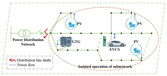
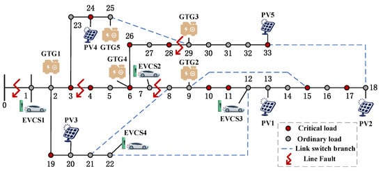
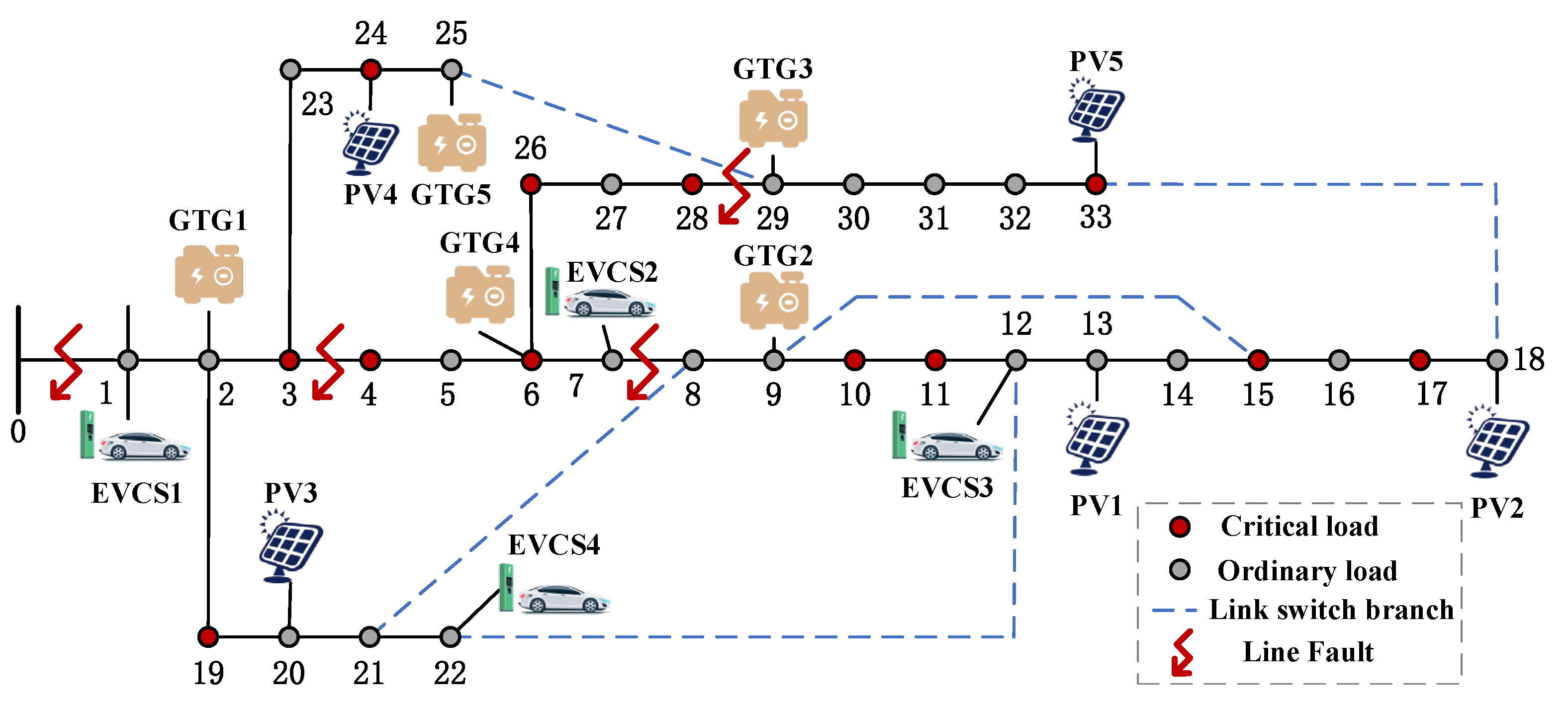
Figure 1 shows the basic layout of the power distribution system, which includes distributed energy resources like PV systems, EVCSs, and GTGs that are connected to the distribution network. To establish a consistent methodological framework, this study systematically divides the resilience enhancement process into two tightly coupled stages: the “pre-disaster robust optimization” stage for strategic planning against uncertainties, and the “post-disaster dynamic scheduling” stage for real-time service restoration. Before the power interruption fault, the centralized grid infrastructure supplied the electrical load demand. Following the disaster, the distribution network was disconnected from the main grid, causing distribution line failures and reducing supply stability.

Figure 1. Schematic structure of the power grid system.

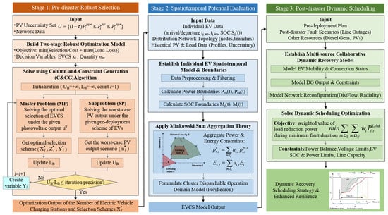
Figure 2 shows that the proposed optimization framework for EVs to make emergency power supply more reliable in distribution systems works by using three different methods:

Figure 2. Framework of V2G-based emergency power supply optimization.

(1)

A two-stage robust optimization model is used to select the most suitable EVCS participants for fault recovery during the planning phase before a disaster. This model considers uncertainties associated with photovoltaic generation and network parameters. The Column-and-Constraint Generation algorithm solves this optimization problem over and over again, which allows the system to respond quickly and restore load after an event.

(2)

In the spatiotemporal operational assessment phase, each EV model is based on when it arrives and leaves, and how much state of charge (SOC) it has. Then, Minkowski sum aggregation methods are used to make a dispatchable operating domain for the EV cluster. This makes it clear what the next steps in the optimization process ought to be.

(3)

A multi-layered collaborative recovery framework is set up during the post-disaster dynamic scheduling phase. This framework puts together EVCSs, network reconfiguration, GTGs, and PV sources. The objective of dynamic scheduling optimization is to reduce load shedding and prioritize restoring critical loads first. This makes the distribution network more robust and resistant.

2.2. Potential Assessment of EVs in V2G Interaction

There are two ways that EVs can regulate their power: up-reserve (discharging to the grid or lowering charging power to lessen frequency dips) and down-reserve (lowering discharge power or raising charging power to lessen frequency surges). There are short-term reserves (lasting from one hour to several hours) and long-term reserves (lasting from one day to several days) based on how long the capacity reserve lasts. The EV’s operational reserve potential changes over time because of factors that depend on time, like real-time charging/discharging power levels and SOC. This means that the reserve capacity changes over time while the EV is in use.

2.2.1. Analysis of Contributing Factors

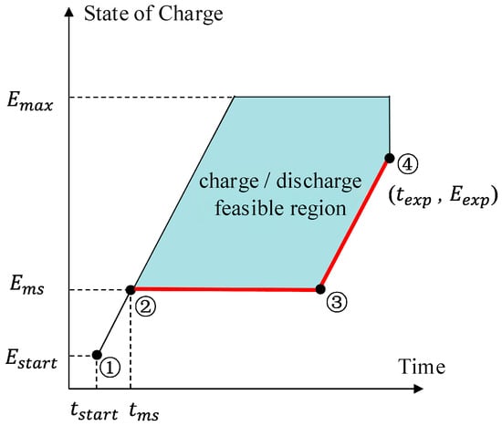
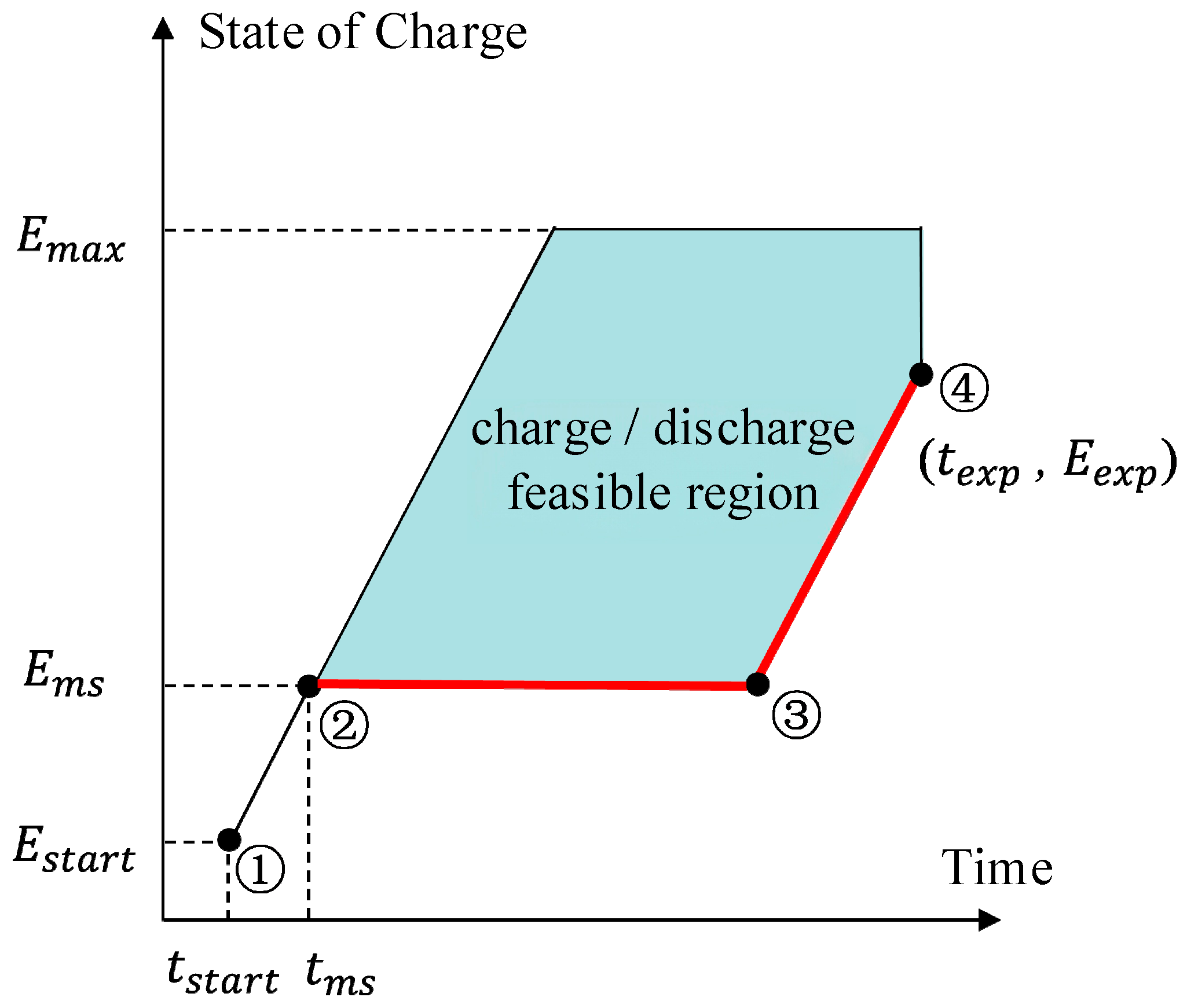
The regulatory capacity of EVs is intrinsically linked to their degree of operational flexibility. As illustrated in Figure 3, the polygonal feasible region is explicitly bounded by the grid-connected time (t_start) and off-grid time (t_exp) on the time axis, and by the battery capacity (E_max) and minimum reserve (E_ms) on the energy axis. The shaded area within these temporal and energetic boundaries represents the operational space available for V2G dispatch, visually correlating the expansion of this domain with increased scheduling adaptability.

Figure 3. Feasible region for EV charging/discharging. Where t_start and t_exp are the EV’s grid-connected and off-grid times specified in the contract, while E_start is the initial battery capacity required for EVs grid connection, E_exp and E_max are the expected power and battery capacity, respectively, for EVs operating off-grid, E_ms and t_ms are the guaranteed minimum power level and the time when charging reaches this threshold.

As depicted in Figure 3, the principal parameters influencing EV charging and discharging processes within this region encompass maximum power throughput for both charging and discharging, battery capacity, minimum reserve capacity, target energy reserves, user travel schedules, real-time charging/discharging rates, SOC, as well as depth of discharge and cycle count, which pertain to battery longevity. Integrating these parameters yields two pivotal operational boundaries defining the EV regulation capacity: the power boundary and the SOC boundary.

(1)

Power Boundary

The power boundary is characterized by the maximum permissible charging and discharging power. When unaffected by the charge constraints, this boundary remains stationary; conversely, it may exhibit dynamic variations contingent upon the charge state and operational conditions.

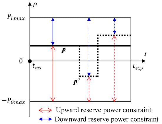
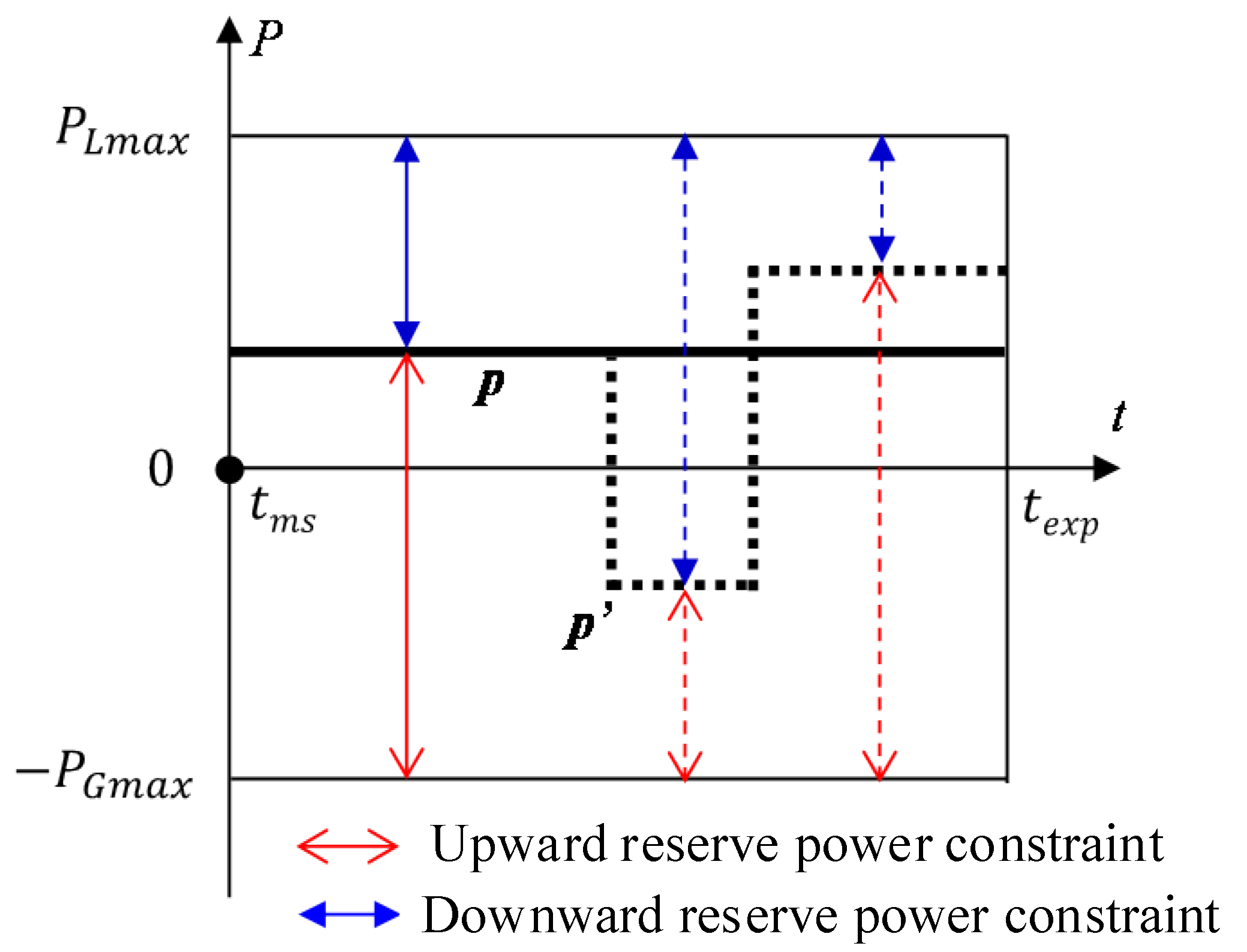
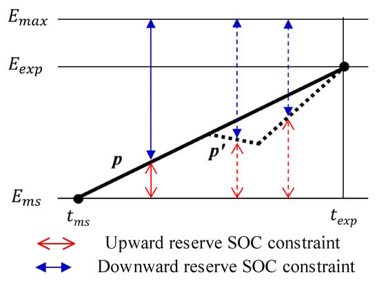
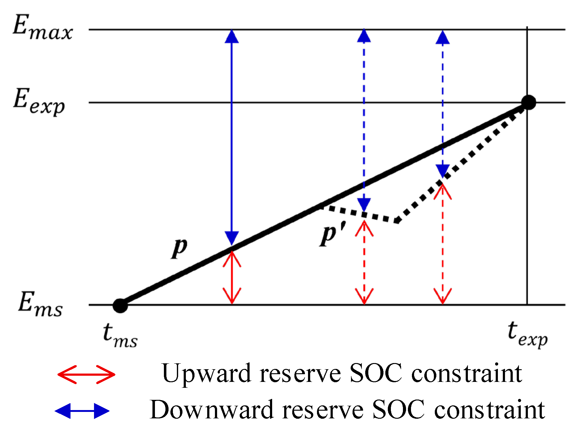
Figure 4 illustrates the impact of maximum charge/discharge power on reserve capacity during typical charging/discharging processes. Specifically, the solid curve p represents the current operating point, while the vertical distances between this curve and the upper/lower power limits ($P_{Lmax}$, $P_{Gmax}$) explicitly quantify the available up/down reserve capacities ($P_{cu}\left(t\right)$, $P_{cd}\left(t\right)$), while the EV’s charge/discharge power is P(t).

$$P\left(t\right)=S_c\left(t\right)P_L\left(t\right)-S_d\left(t\right)P_G\left(t\right)$$

(1)

where P_L(t) and P_G(t) are the real-time charging and discharging power of the charging device; S_c(t) is a binary variable (0 or 1) indicating the EV’s charging status, where S_c(t) = 1 is charging and S_c(t) = 0 is non-charging; S_d(t) is an integer variable in the range (0, 1) that is whether the EV is in a discharge state (S_d(t) = 1) or a non-discharge state (S_d(t) = 0); S_c(t) + S_d(t) ≤ 1.

Figure 4. Effect of Power Constraints on Typical Charge/Discharge.

The EV’s upper and lower reserve capacities must satisfy (2) due to the influence of maximum charge/discharge power.

$$\left\{\begin{array}{c}{P}_{cu}\left(t\right)\le P\left(t\right)+P_{Gmax}\\ P_{cd}\left(t\right)\le P_{Lmax}-P\left(t\right)\\ -P_{Gmax}\le P\left(t\right)\le P_{Lmax}\end{array}\right.$$

(2)

where P_cu(t) is the upper reserve capacity, P_cd(t) is the lower reserve capacity, while P_Lmax and P_Gmax are the maximum charging and discharging power respectively. If the EV’s charging/discharging state changes (as indicated by the black dashed line p’ in Figure 2), the constraints on reserve capacity will also be adjusted accordingly.

(2)

SOC boundary

Power thresholds that can change in real time define the SOC boundary. Changes to the previous dispatching algorithm affect the SOC boundary constraints that come after it. This boundary regulation protocol makes sure that EV dispatching requirements are met, but it makes it harder to control EVs compared to traditional power generation units, especially when keeping peak-shaving capabilities or standby reserves for long periods of time.

Figure 5 illustrates the SOC variations under the charging/discharging power conditions depicted in Figure 4. In this diagram, the SOC trajectory evolves dynamically over time, bounded by the guaranteed minimum level ($E_{ms}$) and the departure requirement. The shaded region delineates the permissible range of battery states, visually demonstrating how energy constraints prevent over-discharge while ensuring sufficient energy for the user’s departure requirements.

Figure 5. SOC Constraint Effect in Typical Charge/Discharge.

To derive the real-time regulation capability, we adopt a step-by-step geometric analysis: the power boundary (Figure 4) first defines the throughput limit, while the energy boundary (Figure 5) subsequently narrows this feasible region to ensure user travel demands are met. Specifically, the battery state $E\left(t\right)$ evolves linearly with power, but constraints become non-linear when the minimum charge requirement must be met before the off-grid time. The real-time battery stage E(t) as a function of the charging/discharging power P(t) is given by (3).

$$E\left(t\right)=E_{start}+{\int }_{t_{start}}^{t}P\left(t\right)dt$$

(3)

Before the battery level drops below the guaranteed minimum, the EV temporarily loses controllability and must be charged at maximum power (P(t) = P_Lmax). Thus, the impact of the battery level boundary can be formalized as (4) to (5).

$$\begin{array}{ll}E\left(t\right)=E_{start}+P_{Lmax}\left(t-t_{start}\right),t\le t_{ms}& \\ E_{ms}\le E\left(t\right)\le E_{max},t_{ms}<t\le t_{exp}& \end{array}$$

(4)

$$E\left(t_{exp}\right)\ge E_{exp}$$

(5)

where t_ms is the time when the battery reaches its minimum guaranteed capacity.

Given the battery’s dependence on maximum charging power, to ensure users’ expected power demands are met within the scheduled timeframe, the battery must maintain a minimum power level during the period from the start of EV regulation to off-grid operation (t_ms~t_exp), as represented by thick solid lines (②~③, ③~④) in Figure 3. The formula for calculating the minimum power at each time can be easily derived, as shown in (6); thus, (4) can be further expressed as (7). Once the battery charge drops to the ③~④ segment in Figure 3, the charging flexibility will vanish immediately. To achieve the desired charge level when the user disconnects from the grid, charging must be initiated at maximum power.

$$E_{min}\left(t\right)=\left\{\begin{array}{ll}{E}_{ms},t_{ms}\le t<\left[t_{exp}-{\displaystyle \frac{E_{exp}-E_{ms}}{P_{Lmax}}}\right]& \\ E_{exp}-P_{Lmax}\left(t_{exp}-t\right),\left[t_{exp}-{\displaystyle \frac{E_{exp}-E_{ms}}{P_{Lmax}}}\right]\le t\le t_{exp}& \end{array}\right.$$

(6)

$$\left\{\begin{array}{ll}E\left(t\right)=E_{start}+P_{L\mathrm{m}\mathrm{a}\mathrm{x}}\left(t-t_{start}\right),t\le t_{ms}& \\ E_{\mathrm{m}\mathrm{i}\mathrm{n}}\left(t\right)\le E\left(t\right)\le E_{\mathrm{m}\mathrm{a}\mathrm{x}},t_{ms}<t\le t_{\mathrm{e}\mathrm{x}\mathrm{p}}& \end{array}\right.$$

(7)

Here, E_min(t) is the real-time minimum power demand.

2.2.2. Individual EV Regulatory Capability Model

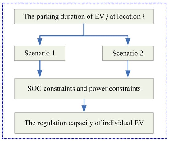
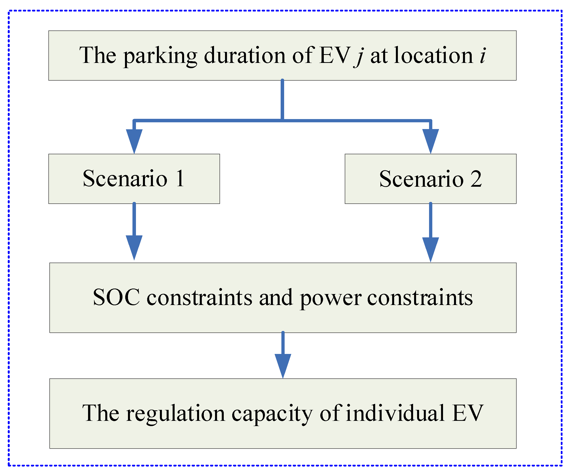
When parked, EVs can participate in grid regulation operations. The EV with serial number j at location i during its parking period constitutes a controllable period. The user arrives at location i at time $t_{j,\mathrm{a}\mathrm{r}\mathrm{r}}^i$, with the corresponding SOC being $S_j\left(t_{j,\mathrm{a}\mathrm{r}\mathrm{r}}^i\right)$; the user departs from i at time $t_{j,\mathrm{l}\mathrm{e}\mathrm{a}}^i$, with the corresponding expected SOC being $S_{j,\mathrm{e}\mathrm{x}\mathrm{p}}^i$; The minimum SOC level that users can accept for regulation is $S_{j,\mathrm{m}\mathrm{i}\mathrm{n}}^i$. Among these,$S_{j,\mathrm{m}\mathrm{i}\mathrm{n}}^i$ must be prioritized. If the SOC of EV at location i is below $S_{j,\mathrm{m}\mathrm{i}\mathrm{n}}^i$, it must first undergo forced charging to the required level $S_{j,\mathrm{m}\mathrm{i}\mathrm{n}}^i$ before accepting any further control commands. The EV’s SOC at arrival time may fall into two scenarios: Scenario 1 ($S_j\left(t_{j,\mathrm{a}\mathrm{r}\mathrm{r}}^i\right)$ is lower than $S_{j,\mathrm{m}\mathrm{i}\mathrm{n}}^i$) and Scenario 2 ($S_j\left(t_{j,\mathrm{a}\mathrm{r}\mathrm{r}}^i\right)$ is higher than $S_{j,\mathrm{m}\mathrm{i}\mathrm{n}}^i$). The regulation capabilities for these scenarios are detailed below, with the technical approach illustrated in Figure 6.

Figure 6. Evaluation Model for Single EV Regulation Potential.

(1)

Regulatory capacity in Scenario 1 ($S_j\left(t_{j,\mathrm{a}\mathrm{r}\mathrm{r}}^i\right)$ is lower than $S_{j,\mathrm{m}\mathrm{i}\mathrm{n}}^i$).

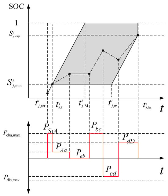
As shown in Figure 7, when the SOC of EV j at location i falls below $S_{j,\mathrm{m}\mathrm{i}\mathrm{n}}^i$ (marked as S₁ in the figure), the EV enters forced charging mode. It charges at maximum power until the specified time $t_{j,f}^i$, at which point the EV’s SOC reaches the target level $S_{j,\mathrm{m}\mathrm{i}\mathrm{n}}^i$, and EV moves into the gray zone in the diagram, transitioning to a non-forced state. Boundary AB represents the EV’s charging process from $S_{j,\mathrm{m}\mathrm{i}\mathrm{n}}^i$ to full capacity at maximum power, with point B corresponding to the time $t_{j,M}^i$. Boundary BC indicates the vehicle’s idle state until departure. Boundary CD defines the SOC range required for the EV’s departure. Boundary AE denotes the EV’s idle state, while boundary ED shows the EV’s forced charging from $S_{j,\mathrm{m}\mathrm{i}\mathrm{n}}^i$ to $S_{j,\mathrm{e}\mathrm{x}\mathrm{p}}^i$ at maximum power, with point E corresponding to the time $t_{j,m}^i$ The gray region bounded by the SOC-t boundary constitutes the controllable region for EV. EV regulation must remain within this region, with its SOC located on the boundary CD at time $t_{j,\mathrm{l}\mathrm{e}\mathrm{a}}^i$.

Figure 7. Schematic diagram of regulatory capacity in Scenario 1.

The upper boundary of the controllable region is defined as A-B-C, which serves as the upper boundary function. For the EV corresponding to sequence number j, its upper boundary at location i is $M_j^i\left(t\right)$. The lower boundary of the controllable region is defined as A-E-D, which serves as the lower boundary function. For the EV corresponding to sequence number j, its lower boundary at location i is $m_j^i\left(t\right)$. The expressions for $M_j^i\left(t\right)$ and $m_j^i\left(t\right)$ are given by (8) and (9):

$$M_j^i\left(t\right)=\left\{\begin{array}{ll}\left(P_{\mathrm{c}\mathrm{h}\mathrm{a},\mathrm{m}\mathrm{a}\mathrm{x}}\cdot t\right)/E_j+\left(S_{j,min}^i\cdot t_{j,M}^i-t_{j,f}^i\right)/\left(t_{j,M}^j-t_{j,f}^i\right)& t_{j,f}^j\le t\le t_{j,M}^j\\ 1& t_{j,M}^i<t\le t_{j,\mathrm{l}\mathrm{e}\mathrm{a}}^i\end{array}\right.$$

(8)

$$m_j^i\left(t\right)=\left\{\begin{array}{ll}{S}_{j,\mathrm{m}\mathrm{i}\mathrm{n}}^i& t_{j,f}^j\le t\le t_{j,m}^j\\ \left(P_{\mathrm{c}\mathrm{h}\mathrm{a},\mathrm{m}\mathrm{a}\mathrm{x}}\cdot t\right)/E_j+\left(S_{j,\mathrm{m}\mathrm{i}\mathrm{n}}^i\cdot t_{j,\mathrm{l}\mathrm{e}\mathrm{a}}^i-S_{j,\mathrm{e}\mathrm{x}\mathrm{p}}^i\cdot t_{j,\mathfrak{m}}^i\right)/\left(t_{j,\mathrm{l}\mathrm{e}\mathrm{a}}^i-t_{j,\mathfrak{m}}^i\right)& t_{j,m}^i<t\le t_{j,\mathrm{l}\mathrm{e}\mathrm{a}}^i\end{array}\right.$$

(9)

The curve A-a-b-c-d-D illustrates EV regulation, where point S ₁to A represents EV charging at maximum power $P_{\mathrm{c}\mathrm{h}\mathrm{a},\mathrm{m}\mathrm{a}\mathrm{x}}$; point A to a indicates EV charging at power $P_{Aa}$; point a to b denotes EV in idle state (neither charging nor discharging); point b to c shows EV charging power $P_{bc}$; point c to d indicates EV reverse discharge at power $P_{cd}$; and point d to D represents EV charging at power $P_{dD}$ until reaching $S_{j,\mathrm{e}\mathrm{x}\mathrm{p}}^i$. Within the EV’s adjustable range and maximum power constraints for charging/discharging, the EV can be regulated according to grid control objectives.

For a single EV with the j-th number, its SOC at time t and location i is

$$S_j\left(t\right)=\left\{\begin{array}{ll}{S}_j\left(t_{j,\mathrm{a}\mathrm{r}\mathrm{r}}^i\right)+{\int }_{t_{j,\mathrm{a}\mathrm{r}\mathrm{r}}^i}^t{P}_{\mathrm{c}\mathrm{h}\mathrm{a},\mathrm{m}\mathrm{a}\mathrm{x}}\mathrm{d}t/E_j& t_{j,\mathrm{a}\mathrm{r}\mathrm{r}}^i\le t\le t_{j,\mathrm{f}}^i\\ S_{j,\mathrm{m}\mathrm{i}\mathrm{n}}^i+{\int }_{t_{j,\mathrm{f}}^i}^t{P}_j\left(t\right)\mathrm{d}t/E_j& t_{j,\mathrm{f}}^i<t\le t_{j,\mathrm{l}\mathrm{e}\mathrm{a}}^i\end{array}\right.$$

(10)

The charge–discharge power of vehicle j is

$$W_j\left(t\right)=\left\{\begin{array}{ll}{P}_{\mathrm{c}\mathrm{h}\mathrm{a},\mathrm{m}\mathrm{a}\mathrm{x}}& t_{j,\mathrm{a}\mathrm{r}\mathrm{r}}^i\le t\le t_{j,\mathrm{f}}^i\\ P_j\left(t\right)& t_{j,\mathrm{f}}^i<t\le t_{j,\mathrm{l}\mathrm{e}\mathrm{a}}^i\end{array}\right.$$

(11)

The adjustable charging capacity of vehicle j at time t is

$$C_{j,\mathrm{d}\mathrm{i}\mathrm{s}}\left(t\right)=\left\{\begin{array}{ll}0& t_{j,\mathrm{a}\mathrm{r}\mathrm{r}}^i\le t\le t_{j,\mathrm{f}}^i\\ \left(S_j\left(t\right)-m_j^i\left(t\right)\right)E_j{H}_j& t_{j,\mathrm{f}}^i<t\le t_{j,\mathrm{l}\mathrm{e}\mathrm{a}}^i\end{array}\right.$$

(12)

The constraints are

$$\left\{\begin{array}{ll}{P}_{\mathrm{d}\mathrm{i}\mathrm{s},\mathrm{m}\mathrm{a}\mathrm{x}}\le P_j\left(t\right)\le P_{\mathrm{c}\mathrm{h}\mathrm{a},\mathrm{m}\mathrm{a}\mathrm{x}}& \\ S_{j,\mathrm{e}\mathrm{x}\mathrm{p}}^i\le S_j\left(t_{j,\mathrm{l}\mathrm{e}\mathrm{a}}^i\right)\le 1& \\ m_j^i\left(t\right)\le S_j\left(t\right)\le M_j^i\left(t\right)& t_{j,\mathrm{f}}^i<t\le t_{j,\mathrm{l}\mathrm{e}\mathrm{a}}^i\end{array}\right.$$

(13)

In Scenario 1, the EV at location i lacks regulation capability and remains in a forced charging state until it goes through duration $t_{j,\mathrm{f}}^i-t_{j,\mathrm{a}\mathrm{r}\mathrm{r}}^i$ to regain regulation capability. If the EV’s parking duration at location i is less than or equal to $t_{j,\mathrm{f}}^i-t_{j,\mathrm{a}\mathrm{r}\mathrm{r}}^i$, it has no regulation capability during this period and is thus an uncontrollable charging load.

(2)

Regulatory capacity in Scenario 2 ($S_j\left(t_{j,\mathrm{a}\mathrm{r}\mathrm{r}}^i\right)$ is higher than $S_{j,\mathrm{m}\mathrm{i}\mathrm{n}}^i$.

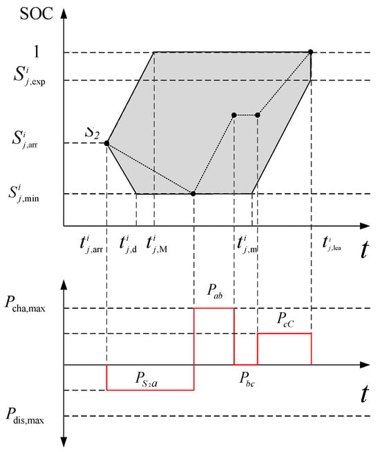
As shown in Figure 8, when the SOC of EV j at location i exceeds $S_{j,\mathrm{m}\mathrm{i}\mathrm{n}}^i$ (marked as S₂ in the diagram), the EV can discharge until its SOC reaches $S_{j,\mathrm{m}\mathrm{i}\mathrm{n}}^i$. Boundary S₂B indicates the EV’s charging from S₂ to full capacity at maximum power, with point B corresponding to the time $t_{j,M}^i$, while boundary S₂A represents the EV’s discharging to $S_{j,\mathrm{m}\mathrm{i}\mathrm{n}}^i$ at maximum power., with point A corresponding to time $t_{j,d}^i$. Boundaries BC, CD, AE, and ED follow the same logic as scenario 1. The gray area bounded by SOC-t defines the EV’s adjustable range, where regulation must always operate within this zone, ensuring the SOC located on boundary CD at time $t_{j,lea}^i$.

Figure 8. Schematic diagram of regulatory capacity in Scenario 2.

The upper boundary of the controllable region is S₂-B-C, and the lower boundary is A-E-D. The upper and lower boundary functions of vehicle j at location i are expressed as (14) and (15).

$$M_j^i\left(t\right)=\left\{\begin{array}{ll}\left(P_{\mathrm{c}\mathrm{h}\mathrm{a},\mathrm{m}\mathrm{a}\mathrm{x}}\cdot t\right)/E_j+\left(S_{j,arr}^i\cdot t_{j,M}^i-t_{j,arr}^i\right)/\left(t_{j,M}^j-t_{j,arr}^i\right)& t_{j,f}^j\le t\le t_{j,M}^j\\ 1& t_{j,M}^i<t\le t_{j,\mathrm{l}\mathrm{e}\mathrm{a}}^i\end{array}\right.$$

(14)

$$m_j^i\left(t\right)=\left\{\begin{array}{ll}\left(P_{\mathrm{d}\mathrm{i}\mathrm{s},\mathrm{m}\mathrm{a}\mathrm{x}}\cdot t\right)/E_j+\left(S_{j,\mathrm{a}\mathrm{r}\mathrm{r}}^i\cdot t_{j,\mathrm{d}}^i-S_{j,\mathrm{m}\mathrm{i}\mathrm{n}}^i\cdot t_{j,\mathrm{a}\mathrm{r}\mathrm{r}}^i\right)/\left(t_{j,\mathrm{d}}^i-t_{j,\mathrm{a}\mathrm{r}\mathrm{r}}^i\right)& t_{j,\mathrm{a}\mathrm{r}\mathrm{r}}^i\le t\le t_{j,\mathrm{d}}^i\\ S_{j,\mathrm{m}\mathrm{i}\mathrm{n}}^i& t_{j,\mathrm{d}}^i<t\le t_{j,\mathrm{m}}^i\\ \left(P_{\mathrm{c}\mathrm{h}\mathrm{a},\mathrm{m}\mathrm{a}\mathrm{x}}\cdot t\right)/E_j+\left(S_{j,\mathrm{m}\mathrm{i}\mathrm{n}}^i\cdot t_{j,\mathrm{l}\mathrm{e}\mathrm{a}}^i-S_{j,\mathrm{e}\mathrm{x}\mathrm{p}}^i\cdot t_{j,\mathfrak{m}}^i\right)/\left(t_{j,\mathrm{l}\mathrm{e}\mathrm{a}}^i-t_{j,\mathfrak{m}}^i\right)& t_{j,m}^i<t\le t_{j,\mathrm{l}\mathrm{e}\mathrm{a}}^i\end{array}\right.$$

(15)

The curve S₂-a-b-c-C illustrates an example of EV regulation, where point S₂ to point a represents EV discharge at power $P_{{\mathrm{s}}_2\mathrm{a}}$, point a to b indicates EV charging at power $P_{\mathrm{a}\mathrm{b}}$, and point b to c denotes EV idle (neither charging nor discharging). From point c to point C, EV charges at power $P_{\mathrm{c}\mathrm{C}}$ until $S_{i,\mathrm{e}\mathrm{x}\mathrm{p}}$. Within the EV’s controllable range and under the maximum power constraints for charging and discharging, the EV can be adjusted according to the grid’s control objectives.

For an EV with the j-th number, its SOC at location i and time t, charge–discharge power, controllable charging and discharging capacity at time t are formulated as (16), and are subject to the constraints given in (17).

$$\left\{\begin{array}{c}{S}_j\left(t\right)=S_j\left(t_{j,\mathrm{a}\mathrm{r}\mathrm{r}}^i\right)+{\int }_{t_{j,\mathrm{a}\mathrm{r}\mathrm{r}}^i}^t{P}_j\left(t\right)dt/E_j t_{j,\mathrm{a}\mathrm{r}\mathrm{r}}^i\le t\le t_{j,\mathrm{l}\mathrm{e}\mathrm{a}}^i\\ \begin{array}{l}{W}_j\left(t\right)=P_j\left(t\right) t_{j,\mathrm{a}\mathrm{r}\mathrm{r}}^i\le t\le t_{j,\mathrm{l}\mathrm{e}\mathrm{a}}^i\\ C_{j,\mathrm{c}\mathrm{h}\mathrm{a}}\left(t\right)=\left(M_j^i\left(t\right)-S_j\left(t\right)\right)E_j{H}_j t_{j,\mathrm{a}\mathrm{r}\mathrm{r}}^i\le t\le t_{j,\mathrm{l}\mathrm{e}\mathrm{a}}^i\\ C_{j,\mathrm{d}\mathrm{i}\mathrm{s}}\left(t\right)=\left(S_j\left(t\right)-m_j^i\left(t\right)\right)E_j{H}_j t_{j,\mathrm{a}\mathrm{r}\mathrm{r}}^i\le t\le t_{j,\mathrm{l}\mathrm{e}\mathrm{a}}^i\end{array}\end{array}\right.$$

(16)

$$\left\{\begin{array}{l}{P}_{\mathrm{d}\mathrm{i}\mathrm{s},\mathrm{m}\mathrm{a}\mathrm{x}}\le P_j\left(t\right)\le P_{\mathrm{c}\mathrm{h}\mathrm{a},\mathrm{m}\mathrm{a}\mathrm{x}}\\ S_{j,\mathrm{e}\mathrm{x}\mathrm{p}}^t\le S_j\left(t_{j,\mathrm{l}\mathrm{e}\mathrm{a}}^t\right)\le 1\\ m_j^t\left(t\right)\le S_j\left(t\right)\le M_j^t\left(t\right) t_{j,\mathrm{a}\mathrm{r}}^t<t\le t_{j,\mathrm{l}\mathrm{e}\mathrm{a}}^t\end{array}\right.$$

(17)

In Scenario 2, the EV at location i has control capability, enabling three operations: charging, discharging, and idle. At this stage, the EV functions as a controllable virtual energy storage device, responding to the grid’s control objectives through corresponding charging and discharging.

2.2.3. EVCS Regulation Capability Model

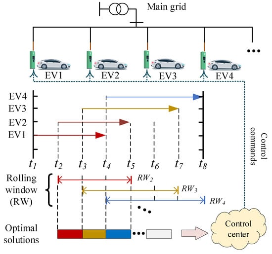
When EVCS participate in emergency power supply, the system optimizes grouping of EVs during the same charging period based on their charging/discharging power. Given the diversity and unpredictability in EV types, charging systems, charging behaviors, and battery SOC, the adjustable potential of EVs and their charging systems exhibits time-varying characteristics and is challenging to predict. To address this, we propose a rolling optimization-based control framework that dynamically adjusts control intervals according to real-time states of EVs and charging stations, as illustrated in Figure 9. For example, assuming four EVs are connected to EVCSs with diversified arrival times and departure times (the coloured arrows represent the corresponding charging time durations in Figure 4), the rolling window length at any instance t, LRW_t, equals the longest remaining charging duration of all available grid-integrated EVs at time instance t, as in (18).

$${LRW}_t=\cup (t_{dep,k}-t),k\in N_t^{ev}$$

(18)

where ${LRW}_t$ represents the rolling window length at time instance t, the expected departure of kth EV is represented by t_dep,k, and the total number of grid-connected EVs at time instance t is represented by $N_t^{ev}$.

Figure 9. Illustration of the rolling-optimization-based control framework of EVs.

The suggested rolling optimization control framework can work with any control time horizon, which meets Minkowski’s requirement that multivariate aggregations belong to a common domain. Minkowski addition, a set operation technique, is used to combine the feasible regions of several geometric or algebraic sets, which shows the boundary of the combined feasible set. In the context of EV fleet scheduling, the power and energy feasibility regions of individual vehicles can be represented as convex sets in a multi-dimensional space. By doing Minkowski sum operations on these sets, a single operational domain for the fleet is created, clearly showing the upper and lower limits of its total regulation capacity [30]. This method works well for allowing vehicles to enter and leave dynamically, and it also gives fleet participation in power grid regulation, precise mathematical limits for optimization, taking into account the fact that constraints can be different and change over time. The application of Minkowski theory to the aggregation of individual EV control capability models facilitates the derivation of the dispatchable power and energy domains of EVCSs, as exemplified in Equation (19).

$$\left\{\begin{array}{ll}\overline{P_{\nu ,t}^{\mathrm{c}}}={\displaystyle \sum _{i\in I_{\nu }}}{u}_{i,t}{P}_{i,t}^{\mathrm{e}\mathrm{v},\mathrm{c}};\overline{P_{\nu ,t}^{\mathrm{d}}}={\displaystyle \sum _{i\in I_{\nu }}}{u}_{i,t}{P}_{i,t}^{\mathrm{e}\mathrm{v},\mathrm{d}}& \\ \underset{\_}{E_{\nu ,t}}={\displaystyle \sum _{i\in I_{\nu }}}{u}_{i,t}\underset{\_}{E_i};\overline{E_{\nu ,t}}={\displaystyle \sum _{i\in I_{\nu }}}{u}_{i,t}\overline{E_i}& \end{array}\right.$$

(19)

Conceptually, this aggregation method simplifies the complex summation of multiple convex sets into a linear superposition of boundary vertices, effectively transforming the distributed fleet into a single virtual energy storage unit characterized by the aggregated bounds.

When considering large-scale EV clusters, multiple EVs may simultaneously connect to or disconnect from the grid, resulting in stepwise electricity fluctuations. To address this issue, the required deviation electricity correction can be determined as shown in (20).

$$∆E_{\nu ,t}=\sum _{i\in I_{\nu }}\left(u_{i,t}\left(1-u_{i,t-1}\right)E_i^{\mathrm{a}\mathrm{r}}-u_{i,t-1}\left(1-u_{i,t}\right)E_i^{\mathrm{e}\mathrm{q}}\right)$$

(20)

where $E_i^{\mathrm{a}\mathrm{r}}$ is the SOC of the i-th EV during grid connection. For the i-th EV, the stepwise electricity fluctuations $∆E_{\nu ,t}$ caused by its transition from grid-connected to off-grid at time t is ${-E}_i^{\mathrm{e}\mathrm{q}}$, while the corresponding $∆E_{\nu ,t}$ when transitioning from off-grid to grid-connected is $E_i^{\mathrm{e}\mathrm{q}}$.

To this end, the schedulable operation domain model composed of EVCSs is shown in (21).

$$\left\{\begin{array}{ll}0\le P_{\nu ,t}^{\mathrm{e}\mathrm{v},\mathrm{c}}\le \overline{P_{\nu ,t}^{\mathrm{c}}}& \\ 0\le P_{\nu ,t}^{\mathrm{e}\mathrm{v},\mathrm{d}}\le \overline{P_{\nu ,t}^{\mathrm{d}}}& \\ P_{\nu ,t}^{\mathrm{e}\mathrm{v},\mathrm{c}\mathrm{d}}={\eta }^{\mathrm{c}}{P}_{\nu ,t}^{\mathrm{e}\mathrm{v},\mathrm{c}}-P_{\nu ,t}^{\mathrm{e}\mathrm{v},\mathrm{d}}/{\eta }^{\mathrm{d}}& \\ E_{\nu ,t}=E_{\nu ,t-1}+P_{\nu ,t}^{\mathrm{e}\mathrm{v},\mathrm{c}\mathrm{d}}∆t+∆E_{\nu ,t}& \\ \underset{\_}{E_{\nu ,t}}\le E_{\nu ,t}\le \overline{E_{\nu ,t}}& \\ E_{\nu ,T}=E_{\nu }^{\mathrm{e}\mathrm{q}}& \end{array}\right.$$

(21)

where $P_{\nu ,t}^{\mathrm{e}\mathrm{v},\mathrm{c}}$ and $P_{\nu ,t}^{\mathrm{e}\mathrm{v},\mathrm{d}}$ are the total charging and discharging power of the EVCS at time t; $P_{\nu ,t}^{\mathrm{e}\mathrm{v},\mathrm{c}\mathrm{d}}$ is the actual interaction power between the EVCS and the grid at time t; $E_{\nu ,t}$ is the total energy storage capacity of the EVCS at time t; $E_{\nu ,T}$ and $E_{\nu }^{\mathrm{e}\mathrm{q}}$ are the actual and expected values of the total battery electricity of the EVCS v at the end of the regulation window T.

It is worth noting that individual EV parameters (e.g., battery capacity $E_j$, arrival and departure times, and SOC) are inherently heterogeneous in practice. The proposed aggregation framework captures this diversity accurately without resorting to complex approximations. Specifically, the individual EV models developed in Section 2.2.2 explicitly derive distinct power and energy boundaries for each vehicle based on its unique physical and behavioral characteristics. As formulated in (19), the Minkowski sum is then applied through direct linear summation of these exact individual upper and lower bounds. Since the constraints of every heterogeneous EV are embedded into their individual boundaries prior to aggregation, the resulting operational envelope inherently and accurately preserves the full diversity of the fleet. This direct summation approach guarantees that any dispatch command within the aggregated bounds can be safely and precisely allocated across heterogeneous EVs without violating their localized physical limits.

From a computational standpoint, a key advantage of the proposed Minkowski sum aggregation is that it mathematically decouples the individual fleet size from the dimensionality of the main optimization problem. Regardless of whether an EVCS serves dozens or thousands of EVs, the aggregation process simply involves the linear summation of individual bounds to construct a single virtual operational domain. As a result, the main MILP solver handles only the aggregated station-level constraints, avoiding the combinatorial explosion associated with tracking discrete state variables for each vehicle. This ensures that the framework remains computationally efficient even for large-scale fleet integration.

2.3. Robust Optimization Model for Pre-Disaster Selection Planning

2.3.1. Objective Function

To determine an optimal and robust EVCS selection strategy for fault recovery under PV output uncertainties, this study develops a two-stage robust optimization model that optimizes the selection of participating EVCSs under the worst-case scenario. The model minimizes the sum of deployment and load shedding costs to determine the optimal number and locations of EVs. The decision-making process comprises two stages: the first stage determines the selection of emergency EVCSs and the distribution network topology (defined by line switch states), while the second stage resolves load shedding levels, DG output, nodal voltages, and branch power flows under the selected EVCS participation scheme. Within this framework, PV output is modeled as an uncertain variable. The objective function is formulated as follows:

$$\underset{{\alpha }_{i,0}^{\mathrm{C}\mathrm{S}},{\alpha }_{ij}}{\mathrm{m}\mathrm{i}\mathrm{n}}\underset{P_i^{\mathrm{P}\mathrm{V}}}{\mathrm{m}\mathrm{a}\mathrm{x}}\underset{\begin{array}{c}{P}_i^{\mathrm{L},\mathrm{s}\mathrm{u}},Q_i^{\mathrm{L},\mathrm{s}\mathrm{u}},P_i^{\mathrm{D}\mathrm{G}},Q_i^{\mathrm{D}\mathrm{G}}\\ P_{ij},Q_{ij},V_i^{\mathrm{s}\mathrm{q}\mathrm{r}},I_{ij}^{\mathrm{s}\mathrm{q}\mathrm{r}}\end{array}}{\mathrm{m}\mathrm{i}\mathrm{n}}\sum _{i\in {\Omega }_B}\left(C^{\mathrm{C}\mathrm{S}}{\alpha }_{i,0}^{\mathrm{C}\mathrm{S}}+{\omega }_i{P}_i^{\mathrm{L},\mathrm{s}\mathrm{u}}\right)$$

(22)

where ${\Omega }_B$ is the set of load nodes; ${\mathrm{C}}^{\mathrm{CS}}$ denotes the comprehensive pre-selection cost per EVCS, serving as baseline compensation for user participation that accounts for anticipated battery degradation during emergency standby; ${\alpha }_{i,0}^{\mathrm{C}\mathrm{S}}$ is a 0–1 variable indicating whether one EVCS is selected, where a value of 1 indicates the EVCS at node i is selected, and a value of 0 means no EVCS is selected; ${\mathsf{\alpha }}_{\mathrm{i}\mathrm{j}}$ is also a 0–1 variable defining the connection status of branch ij, where a value of 1 is the line is closed and a value of 0 is it is open; $P_i^{\mathrm{L},\mathrm{s}\mathrm{u}}$ and $Q_i^{\mathrm{L},\mathrm{s}\mathrm{u}}$ are the active and reactive power reductions in loads; $P_i^{\mathrm{D}\mathrm{G}}$ and $Q_i^{\mathrm{D}\mathrm{G}}$ are the active and reactive outputs of distributed power sources; $P_{ij}$ and $Q_{ij}$ are the active and reactive power of the branch; $V_i^{\mathrm{s}\mathrm{q}\mathrm{r}}$ and $I_{ij}^{\mathrm{s}\mathrm{q}\mathrm{r}}$ are the squared terms of node voltage and branch current; ${\omega }_i$ is the unit load reduction cost of node i; and $P_i^{\mathrm{P}\mathrm{V}}$ is the PV power output, given the real-time volatility of PV generation, its precise value is inherently unpredictable. To develop a robust dispatch strategy capable of handling such uncertainties, this paper adopts a set-box uncertainty $U$ to characterize the potential fluctuation range of PV output relative to predicted values, rather than relying on a single point prediction. The specific formulation is given by the following equation:

$$U=\{\left(1-\tau \right)P_i^{\mathrm{P}\mathrm{V}\ast }\le P_i^{\mathrm{P}\mathrm{V}}\le P_i^{\mathrm{P}\mathrm{V}\ast }\}$$

(23)

where $P_i^{\mathrm{P}\mathrm{V}\ast }$ is the predicted PV output and $\tau$ is the uncertainty, which is the scaling ratio of the uncertainty set.

In the pre-disaster EVCS pre-selection stage of the two-stage robust optimization model, the scheduling logic emphasizes practical engineering constraints and multi-criteria considerations. Selection is based on three core factors: (1) heterogeneity in regulation potential, quantified by a Minkowski summation-based method accounting for variations in vehicle types, parking durations, and initial SOC distributions; (2) spatial proximity to critical loads, prioritizing EVCSs near high-cost nodes to reduce transmission losses and enhance emergency response; (3) economic viability, incorporating a unit subsidy of 500 CNY and minimizing total pre-deployment costs to balance regulation capacity, spatial distribution, and cost-effectiveness, thus ensuring readiness for rapid post-disaster recovery.

2.3.2. Stage 1 Constraints

(1)

Resource constraints for EVCSs. Given the limited number of EVCSs available for grid emergency response before disasters and their identical charging and discharging parameters, the selection scope of EVCSs is constrained. This limitation can be mathematically represented as:

$$\sum _{i\in {\Omega }_{\mathrm{B}}}{\alpha }_{i,0}^{\mathrm{C}\mathrm{S}}\le N_{\mathrm{m}\mathrm{a}\mathrm{x}}^{\mathrm{C}\mathrm{S}}$$

(24)

where $N_{\mathrm{m}\mathrm{a}\mathrm{x}}^{\mathrm{C}\mathrm{S}}$ is the maximum number of EVCSs planned during the pre-selection phase.

(2)

Radial operation constraints for distribution networks: To account for island integration and power-free island scenarios, the improved single-commodity flow method is adopted. By introducing 0–1 variables to virtual source node markers, the number of islands is incorporated into the optimization process. The virtual power flow is relaxed using the Big-M method, as detailed below:

$$\left\{\begin{array}{c}{\displaystyle \sum _{ij\in {\Omega }_{\mathrm{B}}}}{\alpha }_{ij}=N_{\mathrm{B}}-{\displaystyle \sum _{i\in {\Omega }_{\mathrm{N}}}}{S}_i^{\mathrm{V}\mathrm{S}}\\ {\displaystyle \sum _{j\in \delta \left(i\right)}}{F}_{ij}-{\displaystyle \sum _{k\in \gamma \left(i\right)}}{F}_{ki}=F_i^{\mathrm{V}\mathrm{S}}-1\\ -M_k{S}_i^{\mathrm{V}\mathrm{S}}\le F_i^{\mathrm{V}\mathrm{S}}\le M_k{S}_i^{\mathrm{V}\mathrm{S}}\\ -M_{\mathrm{k}}{\alpha }_{ij}\le F_{ij}\le M_k{\alpha }_{ij}\end{array}\right.$$

(25)

where ${\Omega }_{\mathrm{B}}$ is the set of system branches; $N_B$ is the total number of system nodes; $\delta \left(i\right)$ and $\gamma \left(i\right)$ are the set of branches terminating at node i and those originating from node i; $F_{ij}$ is the virtual power flow on branch ij; $F_i^{VS}$ is the virtual power generated by node i; and $M_k$ is a sufficiently large positive real number serving as the parameter for the Big-M method in the model.

2.3.3. Stage 2 Constraints

(1)

Load reduction constraint. To maintain a constant power factor during load reduction, the reduction in active and reactive power must follow a specific proportional relationship. This constraint can be expressed as

$$\left\{\begin{array}{c}0\le P_i^{L,su}\le P_{i,max}^L\\ Q_i^{Lsu}={\displaystyle \frac{Q_{i,max}^L}{P_{i,max}^L}}{P}_i^{Lsu}\end{array}\right.$$

(26)

where $P_{i,\mathrm{m}\mathrm{a}\mathrm{x}}^{\mathrm{L}}$ and $Q_{i,\mathrm{m}\mathrm{a}\mathrm{x}}^{\mathrm{L}}$ are the maximum active and reactive power loads.

(2)

Constraints on DG. The rated power output of DG units at each node must not exceed their specified capacity limits. For flexible resources such as EVs, their available energy output capacity depends on their initial state of charge; assuming these vehicles are fully charged prior to an emergency, the maximum charge–discharge power delineates the upper boundary of their power contribution. Furthermore, DG systems must adhere to prescribed operational relationships among active power, reactive power, and power factor, with PV systems implementing constant power factor control strategies. The operational constraints for DG can be formally specified as follows:

$$\left\{\begin{array}{c}-{\displaystyle \sum _{i\in \{E,G,P\}}}{\alpha }_i^{\mathrm{D}\mathrm{G}}{P}_{i,\mathrm{m}\mathrm{a}\mathrm{x}}^{\mathrm{D}\mathrm{G}}\le P_i^{\mathrm{D}\mathrm{G}}\le {\displaystyle \sum _{i\in \{E,G,P\}}}{\alpha }_i^{\mathrm{D}\mathrm{G}}{P}_{i,\mathrm{m}\mathrm{a}\mathrm{x}}^{\mathrm{D}\mathrm{G}}\\ -{\displaystyle \sum _{i\in \{E,G,P\}}}{\alpha }_i^{\mathrm{D}\mathrm{G}}{Q}_{i,\mathrm{m}\mathrm{a}\mathrm{x}}^{\mathrm{D}\mathrm{G}}\le Q_i^{\mathrm{D}\mathrm{G}}\le {\displaystyle \sum _{i\in \{E,G,P\}}}{\alpha }_i^{\mathrm{D}\mathrm{G}}{Q}_{i,\mathrm{m}\mathrm{a}\mathrm{x}}^{\mathrm{D}\mathrm{G}}\\ cos{\phi }_{i,\mathrm{m}\mathrm{i}\mathrm{n}}^{\mathrm{D}\mathrm{G}}\le {\displaystyle \frac{P_i^{\mathrm{D}\mathrm{G}}}{\sqrt{{\left(P_i^{\mathrm{D}\mathrm{G}}\right)}^2+{\left(Q_i^{\mathrm{D}\mathrm{G}}\right)}^2}}}\le cos{\phi }_{i,\mathrm{m}\mathrm{a}\mathrm{x}}^{\mathrm{D}\mathrm{G}}\end{array}\right.$$

(27)

where E, G, and P are the node sets for EVCSs, GTGs, and PV systems, respectively; ${\alpha }_i^{\mathrm{D}\mathrm{G}}$ is the connection status between the distributed power sources and node i; $P_{i,\mathrm{m}\mathrm{a}\mathrm{x}}^{\mathrm{D}\mathrm{G}}$ and $Q_{i,\mathrm{m}\mathrm{a}\mathrm{x}}^{\mathrm{D}\mathrm{G}}$ are the upper limits of active and reactive power output for distributed power sources; and $\mathrm{c}\mathrm{o}\mathrm{s}{\phi }_{i,\mathrm{m}\mathrm{i}\mathrm{n}}^{\mathrm{D}\mathrm{G}}$ and $\mathrm{c}\mathrm{o}\mathrm{s}{\phi }_{i,\mathrm{m}\mathrm{a}\mathrm{x}}^{\mathrm{D}\mathrm{G}}$ are the upper and lower limits of power factor for distributed power sources, with identical parameters for PV systems.

(3)

Distribution network operation constraints. To accurately model the operational state of radial distribution networks, the DistFlow power flow equations serve as the fundamental framework. However, given that network topology dynamically changes with line switch states, resulting in nonlinear power flow equations, the Big-M method is employed to linearize and relax critical voltage constraints. The system operation constraints can be formulated as follows:

$$\left\{\begin{array}{c}{\displaystyle \sum _{j\in \delta \left(i\right)}}{P}_{ij}-{\displaystyle \sum _{j\in \gamma \left(i\right)}}\left(P_{ji}-R_{ji}{I}_{ji}^{\mathrm{s}\mathrm{q}\mathrm{r}}\right)=P_i^{\mathrm{D}\mathrm{G}}-P_{i,\mathrm{m}\mathrm{a}\mathrm{x}}^{\mathrm{L}}+P_i^{\mathrm{L}\mathrm{s}\mathrm{u}}\\ {\displaystyle \sum _{j\in \delta \left(i\right)}}{Q}_{ij}-{\displaystyle \sum _{j\in \gamma \left(i\right)}}\left(Q_{ji}-X_{ji}{I}_{ji}^{sqr}\right)=Q_i^{\mathrm{D}\mathrm{G}}-Q_{i,\mathrm{m}\mathrm{a}\mathrm{x}}^{\mathrm{L}}+Q_i^{\mathrm{L}\mathrm{s}\mathrm{u}}\\ V_i^{\mathrm{s}\mathrm{q}\mathrm{r}}-V_j^{\mathrm{s}\mathrm{q}\mathrm{r}}-2\left(R_{ij}{P}_{ij}+X_{ij}{Q}_{ij}\right)+\left(R_{ij}^2+X_{ij}^2\right){\displaystyle \frac{P_{ij}^2+Q_{ij}^2}{V_i^{\mathrm{s}\mathrm{q}\mathrm{r}}}}\le M_k\left(1-{\alpha }_{ij}\right)\\ V_i^{\mathrm{s}\mathrm{q}\mathrm{r}}-V_j^{\mathrm{s}\mathrm{q}\mathrm{r}}-2\left(R_{ij}{P}_{ij}+X_{ij}{Q}_{ij}\right)+\left(R_{ij}^2+X_{ij}^2\right){\displaystyle \frac{P_{ij}^2+Q_{ij}^2}{V_i^{\mathrm{s}\mathrm{q}\mathrm{r}}}}\ge M_1\left({\alpha }_{ij}-1\right)\\ V_{i,\mathrm{m}\mathrm{i}\mathrm{n}}^{\mathrm{s}\mathrm{q}\mathrm{r}}\le V_i^{\mathrm{s}\mathrm{q}\mathrm{r}}\le V_{i,\mathrm{m}\mathrm{a}\mathrm{x}}^{\mathrm{s}\mathrm{q}\mathrm{r}}\\ 0\le I_{ij}^{\mathrm{s}\mathrm{q}\mathrm{r}}\le {\alpha }_{ij}{I}_{ij,\mathrm{m}\mathrm{a}\mathrm{x}}^{\mathrm{s}\mathrm{q}\mathrm{r}}\\ P_{ij}^2+Q_{ij}^2\le V_i^{\mathrm{s}\mathrm{q}\mathrm{r}}{I}_{ij}^{\mathrm{s}\mathrm{q}\mathrm{r}}\end{array}\right.$$

(28)

where $R_{ji}$ and $X_{ji}$ are the branch resistance and reactance, respectively; $V_{i,\mathrm{m}\mathrm{a}\mathrm{x}}^{\mathrm{s}\mathrm{q}\mathrm{r}}$ and $V_{i,\mathrm{m}\mathrm{i}\mathrm{n}}^{\mathrm{s}\mathrm{q}\mathrm{r}}$ are the upper and lower bounds of the node voltage squared terms; and $I_{ij,\mathrm{m}\mathrm{a}\mathrm{x}}^{\mathrm{s}\mathrm{q}\mathrm{r}}$ is the upper limit of the branch current squared term.

For nonlinear constraints among voltage, current, and power, the second-order cone relaxation method is applied to transform them into the following second-order cone constraints:

$${‖\begin{array}{c}2P_{ij}\\ 2Q_{ij}\\ I_{ij}^{\mathrm{s}\mathrm{q}\mathrm{r}}-V_i^{\mathrm{s}\mathrm{q}\mathrm{r}}\end{array}‖}_2\le I_{ij}^{\mathrm{s}\mathrm{q}\mathrm{r}}+V_i^{\mathrm{s}\mathrm{q}\mathrm{r}}$$

(29)

2.3.4. Model Solving Algorithm

For the two-stage robust optimization model in the pre-disaster robust optimization stage, the column constraint generation (C&CG) algorithm is used to solve the problem. The compact form of the original problem is as follows:

$$\left\{\begin{array}{c}\begin{array}{l}\underset{x}{\mathrm{m}\mathrm{i}\mathrm{n}}\underset{u\in U_s}{\mathrm{m}\mathrm{a}\mathrm{x}}\underset{Y\in \Omega \left(X,u\right)}{\mathrm{m}\mathrm{i}\mathrm{n}}{b}^{\mathrm{T}}Y\\ \mathrm{s}.\mathrm{t}. AX\le a\\ \Omega \left(X,u\right)=\left\{Y\mid BY\ge CX,DY=u,\right.\end{array}\\ \left. \parallel E_{m}Y{\parallel }_2\le f_m^{\mathrm{T}}Y,m=1,2,\cdots ,n\right\}\end{array}\right.$$

(30)

where $x$ is the optimization variable of the first stage, $u$ and $Y$ are the optimization variables of the second stage, $U_s$ is the uncertainty set, $\Omega \left(X,u\right)$ is the feasible region of variable $Y$, $A$, $B$, $C$, $D$, $E_m$ are constant coefficient matrices, $a$, $b$ and $f_m$ are coefficient vectors, and $n$ is the number of second-order cone constraints.

Then, the original problem is decomposed into a master problem and a subproblem, where the master problem is to solve the optimal pre-deployment scheme of EVs under the given PV output u*, as shown in Equation (31). This mixed integer second-order cone programming problem can be solved by commercial solvers.

$$\left\{\begin{array}{ll}\underset{X,\mathrm{Z}}{\mathrm{m}\mathrm{i}\mathrm{n} }& c^{\mathrm{T}}\mathrm{X}+\mathrm{Z}\\ \mathrm{s}.\mathrm{t}.& A\mathrm{X}\le a\\ & \mathrm{Z}\ge b^{\mathrm{T}}{\mathrm{Y}}_l,\forall l\le K\\ & B{\mathrm{Y}}_l\ge C\mathrm{X},\forall l\le K\\ & D{\mathrm{Y}}_l={\mathrm{u}}_l^{*},\forall l\le K\\ & {∥E_m{\mathrm{Y}}_l∥}_2\le f_m^{\mathrm{T}}{\mathrm{Y}}_l,m=\mathrm{1,2},\cdots ,n,\forall l\le K\end{array}\right.$$

(31)

where $\mathrm{Z}$ is the auxiliary variable, $K$ is the maximum number of iterations, and the subscript $l$ is the variable obtained in the $l$-th iteration.

The subproblem solving for the worst-case PV output under the given pre-deployment scheme ${\mathrm{X}}^{\ast }$ of EVs, which is defined as

$$\left\{\begin{array}{ll}\underset{u}{\mathrm{m}\mathrm{a}\mathrm{x} }\underset{Y}{\mathrm{m}\mathrm{i}\mathrm{n} }& b^{\mathrm{T}}\mathrm{Y}\\ \mathrm{s}.\mathrm{t}.& \mathrm{Z}\ge b^{\mathrm{T}}Y,\forall l\le K\\ & B\mathrm{Y}\ge C{\mathrm{X}}^{\ast },\forall l\le K\\ & D{\mathrm{Y}}_l=u,\forall l\le K\\ & {∥E_{m}Y∥}_2\le f_m^{\mathrm{T}}Y,m=\mathrm{1,2},\cdots ,n,\forall l\le K\end{array}\right.$$

(32)

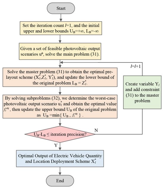
The subproblems can be solved by commercial solvers, and the C&CG algorithm for the two-stage robust optimization model is shown in Figure 10.

Figure 10. Solution flowchart of C&CG algorithm.

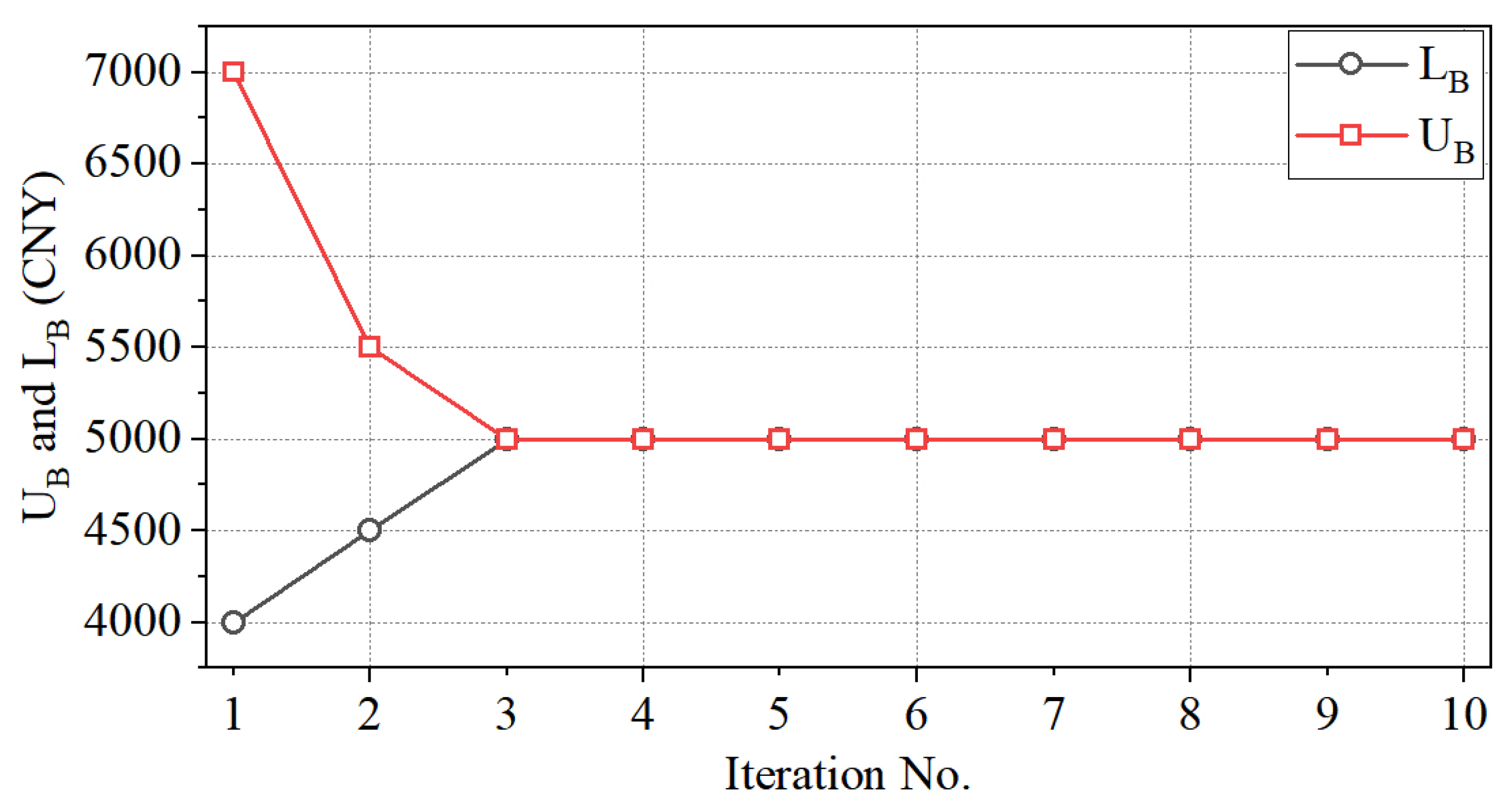
The C&CG algorithm iteratively narrows the gap between the upper bound U_B from the subproblem and the lower bound L_B from the master problem, and is known to converge to the global optimum within a finite number of iterations. The solution process stops once the relative optimality gap falls below a predefined tolerance $\epsilon$, expressed as: $\left|U_B-L_B\right|\le \epsilon$. In this study, the convergence tolerance $\epsilon$ is strictly set to 10⁻⁴ to ensure accurate numerical solutions.

This study employs the commercial solver Gurobi to address both the main and sub-problems in two-stage robust optimization. The solver demonstrates significant efficiency and precision advantages in solving mixed-integer second-order conic programming problems, while supporting customized iteration logic to efficiently meet the requirements of the C&CG algorithm, ensuring rapid generation of planning solutions under extreme scenarios. For the subsequent disaster recovery model involving multi-source collaborative dynamic restoration, its sparse matrix processing capabilities and parallel computing support for large-scale mixed-integer linear programming problems guarantee real-time and globally optimal scheduling results within 10 h for fault scenarios, meeting the time-sensitive demands of post-disaster emergency dispatch.

2.4. Multi-Source Collaborative Post-Disaster Recovery Optimization Model

2.4.1. Objective Function

Following a catastrophic failure, the distribution system is isolated from the main grid, with the outage duration depending on the severity of the incident and the availability of repair resources. To balance resilience enhancement with the economic preservation of EV battery life cycles, a degradation cost $c_{deg}$ is introduced and embedded into the operational objective. This ensures that EVs are dispatched only when their contribution to reducing high-penalty load shedding $w_i$ outweighs the associated battery aging cost. Based on the above, a multi-agent collaborative post-disaster recovery optimization framework is developed to minimize weighted load shedding during restoration while safeguarding EV battery longevity. The framework coordinates the dynamic dispatch of EVCS and GTGs to improve the robustness and resilience of the distribution network. The objective function is formulated as follows:

$$\left\{\begin{array}{c}\mathrm{m}\mathrm{i}\mathrm{n}{\displaystyle \sum _{t\in {\Omega }_{\mathrm{T}}}}\left({\displaystyle \sum _{i\in {\Omega }_{\mathrm{N}}}}{w}_i{P}_{i,t}^{\mathrm{L}\mathrm{s}\mathrm{h}\mathrm{d}}+{\displaystyle \sum _{i\in {\Omega }_{\mathrm{C}\mathrm{S}}}}{c}_{\mathrm{d}\mathrm{e}\mathrm{g}}{P}_{i,t}^{\mathrm{C}\mathrm{d}\mathrm{c}\mathrm{h}}∆t\right)\\ c_{\mathrm{d}\mathrm{e}\mathrm{g}}={\displaystyle \frac{C_{\mathrm{r}\mathrm{e}\mathrm{p}}}{N_{\mathrm{c}\mathrm{y}\mathrm{c}\mathrm{l}\mathrm{e}}}}·E_{i,\mathrm{m}\mathrm{a}\mathrm{x}}^{\mathrm{C}\mathrm{S}}·DOD\end{array}\right.$$

(33)

where ${\Omega }_{\mathrm{T}}$ is the set of fault periods, $P_{i,t}^{\mathrm{L}\mathrm{s}\mathrm{h}\mathrm{d}}$ is the active power reduction load at node i during time t; $c_{deg}$ represents the unit degradation cost of the EV battery due to V2G discharging; $C_{rep}$ is the total replacement cost of the EV battery; $N_{cycle}$ denotes the expected cycle life of the battery under nominal operations; $E_{i,max}^{CS}$ is the rated energy capacity of the participating EV; and $DOD$ represents the operational depth of discharge. this linearized formulation ensures that EV discharging is economically justified only when the value of avoided load shedding compensates for the internalized cost of battery wear; to accommodate the dispatch time scale under disaster scenarios, the dispatch interval is set to 1 h.

The decision variables in this phase include the selection status ${\alpha }_{i,j,t}^{\mathrm{C}\mathrm{S}}$ of EVCS at each time period; the active power output $P_{i,\mathrm{t}}^{\mathrm{D}\mathrm{G}}$ and reactive power output $Q_{i,\mathrm{t}}^{\mathrm{D}\mathrm{G}}$ of DG; the state of energy $E_{i,t}^{\mathrm{E}\mathrm{V}}$ and charging/discharging power $P_{i,t}^{\mathrm{C}\mathrm{d}\mathrm{c}\mathrm{h}}$ of EVs connected to charging stations; and the active power reduction $P_{i,\mathrm{t}}^{\mathrm{L}\mathrm{s}\mathrm{u}}$ and reactive power reduction $Q_{i,\mathrm{t}}^{\mathrm{L}\mathrm{s}\mathrm{u}}$ of load.

2.4.2. Constraints

(1)

Dynamic scheduling constraints of EVCSs.

The coupling relationship between the pre-disaster selection phase and the disaster recovery stage is described by (34), ensuring the proper dispatch of pre-selected EVCS during disaster events.

$$\sum _{i\in {\Omega }_{EV}}{\alpha }_{i,j,t_0}^{\mathrm{C}\mathrm{S}}={\alpha }_{j,0}^{\mathrm{C}\mathrm{S}}$$

(34)

Here, ${\Omega }_{CS}$ is the pre-selected EVCSs prior to the disaster; $t_0$ is the fault occurrence time.

The coupling between EVCSs’ charging and discharging states and their spatial configurations is established by (35), ensuring they perform charging and discharging during selection states.

$$U_{i,t}^{\mathrm{C}\mathrm{c}\mathrm{h}}+U_{i,t}^{\mathrm{C}\mathrm{d}\mathrm{c}\mathrm{h}}\le \sum _{j\in {\Omega }_N}{\alpha }_{i,j,t}^{\mathrm{C}\mathrm{S}}{\alpha }_{i,j,t+1}^{\mathrm{C}\mathrm{S}}$$

(35)

Here, $U_{i,t}^{\mathrm{C}\mathrm{c}\mathrm{h}}$ and $U_{i,t}^{\mathrm{C}\mathrm{d}\mathrm{c}\mathrm{h}}$ are the charging and discharging indicators for EVCSs, with values of 1 representing the charging and discharging states.

As (35) contains bilinear terms, a linearization approach is applied to transform it into the following linear constraints:

$$\left\{\begin{array}{l}{\alpha }_{i,j,t}^{\mathrm{C}\mathrm{C}\mathrm{S}}\le {\alpha }_{i,j,t+1}^{\mathrm{C}\mathrm{S}}\\ {\alpha }_{i,j,t}^{\mathrm{C}\mathrm{C}\mathrm{S}}\le {\alpha }_{i,j,t}^{\mathrm{C}\mathrm{S}}\\ {\alpha }_{i,j,t}^{\mathrm{C}\mathrm{C}\mathrm{S}}\ge {\alpha }_{i,j,t+1}^{\mathrm{C}\mathrm{S}}+{\alpha }_{i,j,t+1}^{\mathrm{C}\mathrm{C}\mathrm{S}}-1\\ U_{i,t}^{\mathrm{C}\mathrm{c}\mathrm{h}}+U_{i,t}^{\mathrm{C}\mathrm{d}\mathrm{c}\mathrm{h}}\le {\displaystyle \sum _{j\in {\Omega }_N}}{\alpha }_{i,j,t}^{\mathrm{C}\mathrm{C}\mathrm{S}}\end{array}\right.$$

(36)

where ${\alpha }_{i,j,t}^{\mathrm{C}\mathrm{C}\mathrm{S}}$ is an introduced intermediate variable indicating the connection status between EVCS i and node j during the period t~(t+1).

The upper and lower bounds for active and reactive power in EVCS charging and discharging are defined by (37):

$$\left\{\begin{array}{c}0\le P_{i,t}^{\mathrm{C}\mathrm{ch}}\le U_{i,t}^{\mathrm{C}\mathrm{ch}}{P}_{i,t,\mathrm{m}\mathrm{a}\mathrm{x}}^{\mathrm{C}\mathrm{ch}}\\ 0\le P_{i,t}^{\mathrm{C}\mathrm{dch}}\le U_{i,t}^{\mathrm{C}\mathrm{dch}}{P}_{i,t,\mathrm{m}\mathrm{a}\mathrm{x}}^{\mathrm{C}\mathrm{dch}}\\ 0\le Q_{i,t}^{\mathrm{C}\mathrm{ch}}\le U_{i,t}^{\mathrm{C}\mathrm{ch}}{Q}_{i,t,\mathrm{m}\mathrm{a}\mathrm{x}}^{\mathrm{C}\mathrm{ch}}\\ 0\le Q_{i,t}^{\mathrm{C}\mathrm{dch}}\le U_{i,t}^{\mathrm{C}\mathrm{dch}}{Q}_{i,t,\mathrm{m}\mathrm{a}\mathrm{x}}^{\mathrm{C}\mathrm{dch}}\end{array}\right.$$

(37)

where $P_{i,t}^{\mathrm{C}\mathrm{ch}}$ and $P_{i,t}^{\mathrm{C}\mathrm{dch}}$ are active power during charging and discharging; $Q_{i,t}^{\mathrm{C}\mathrm{ch}}$ and $Q_{i,t}^{\mathrm{C}\mathrm{dch}}$ are reactive power for charging and discharging of EVCSs; $P_{i,t,\mathrm{m}\mathrm{a}\mathrm{x}}^{\mathrm{C}\mathrm{ch}}$ and $P_{i,t,\mathrm{m}\mathrm{a}\mathrm{x}}^{\mathrm{C}\mathrm{dch}}$ are upper limits for active power consumption during charging and discharging; $Q_{i,t,\mathrm{m}\mathrm{a}\mathrm{x}}^{\mathrm{C}\mathrm{ch}}$ and $Q_{i,t,\mathrm{m}\mathrm{a}\mathrm{x}}^{\mathrm{C}\mathrm{dch}}$ are upper limits for reactive power consumption during charging and discharging.

Constraints on the station’s SOC are imposed by (38):

$$\left\{\begin{array}{c}{E}_{i,t+∆t}^{CS}=E_{i,t}^{CS}+P_{i,t}^{Cch}{\eta }_i^{Cch}∆t-{\displaystyle \frac{P_{i,t}^{Cdch}}{{\eta }_i^{Cdch}}}∆t\\ E_{i,min}^{CS}\le E_{i,t}^{CS}\le E_{i,max}^{CS}\end{array}\right.$$

(38)

where ${\eta }_i^{\mathrm{C}\mathrm{c}\mathrm{h}}$ and ${\eta }_i^{\mathrm{C}\mathrm{d}\mathrm{c}\mathrm{h}}$ are charging and discharging efficiency of EVCSs; $E_{i,\mathrm{m}\mathrm{a}\mathrm{x}}^{\mathrm{C}\mathrm{S}}$ and $E_{i,\mathrm{m}\mathrm{i}\mathrm{n}}^{\mathrm{C}\mathrm{S}}$ are upper and lower limits for energy storage capacity of EVCSs.

(2)

Other constraints.

In the post-disaster recovery phase, the load reduction power, distributed power generation output, and distribution network operation at each time point must still comply with corresponding constraints. The form of these constraints is the same as in the pre-disaster pre-planning stage, as shown in (26) to (29).

3. Results

3.1. Basic Information on System Under Test

This study employs the enhanced IEEE 33-bus distribution network depicted in Figure 11 for simulation analysis. A power disruption disaster was initiated at 04:00, resulting in failures affecting the upper-level power grid and the following distribution lines: 0–1, 3–4, 7–8, and 28–29. The duration of the fault was specified as 10 h. Before the power disruption disaster, all electric vehicles were charged following their users’ habits, with the vehicle types considered and their proportional distributions detailed in Table 1. The EVCSs, DGs, load, and system operation parameters are detailed in Table 2, Table 3, Table 4 and Table 5.

Figure 11. Structure of modified IEEE 33-bus distribution network.

Table 1. Vehicle type and proportion configuration.

Vehicle Type	Quantity	Proportion
Private	80	40%
Ride_hailing	70	35%
Taxi	40	20%
Bus	10	5%

Table 2. Operating Parameters of EVCSs.

Power Supply	Maximum Active Power/kW	Maximum Reactive Power/kVAr	Charge–Discharge Efficiency	Energy Storage Capacity/kWh
EVCS1, EVCS2, EVCS3, EVCS4	600	510	0.98	1800

Table 3. Operating Parameters of DGs.

Power Supply	Maximum Active Power/kW	Maximum Reactive Power/kVAr
GTG1, GTG2, GTG3	120	±100
GTG4, GTG5	80	±60
PV1	100	±96
PV2	240	±192
PV3, PV4	360	±288
PV5	180	±144

Table 4. Operating Parameters of Loads.

Node	Unit Load Reduction Cost (CNY)	Active Power/kW	Reactive Power/kvar
1	1	60	30
2	1	100	60
3	10	90	40
4	10	120	80
5	1	60	30
6	10	60	20
7	1	200	100
8	1	200	100
9	1	60	20
10	10	60	20
11	10	45	30
12	1	60	35
13	1	60	35
14	1	120	80
15	10	60	10
16	1	60	20
17	10	60	20
18	1	90	40
19	10	90	40
20	1	90	40
21	1	90	40
22	1	90	40
23	1	90	50
24	10	420	200
25	1	420	200
26	10	60	25
27	1	60	25
28	10	40	20
29	1	120	70
30	1	200	600
31	1	150	70
32	1	210	100
33	10	60	40
Total	/	3605	2300

Table 5. Parameters of system operation.

Parameter	Numerical Value
Rated voltage	12.66 kV
Voltage upper limit	13.92 kV
Voltage lower limit	11.39 kV
Unit selection cost of emergency EVCSs	500 CNY
$\mathrm{Uncertainty} \tau$	0.35

In Table 4, loads with higher cost reductions are classified as critical loads, while the remaining loads are categorized as non-critical loads.

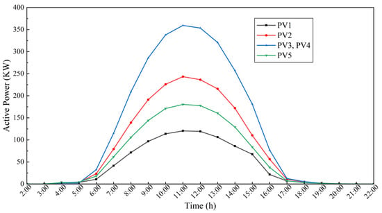
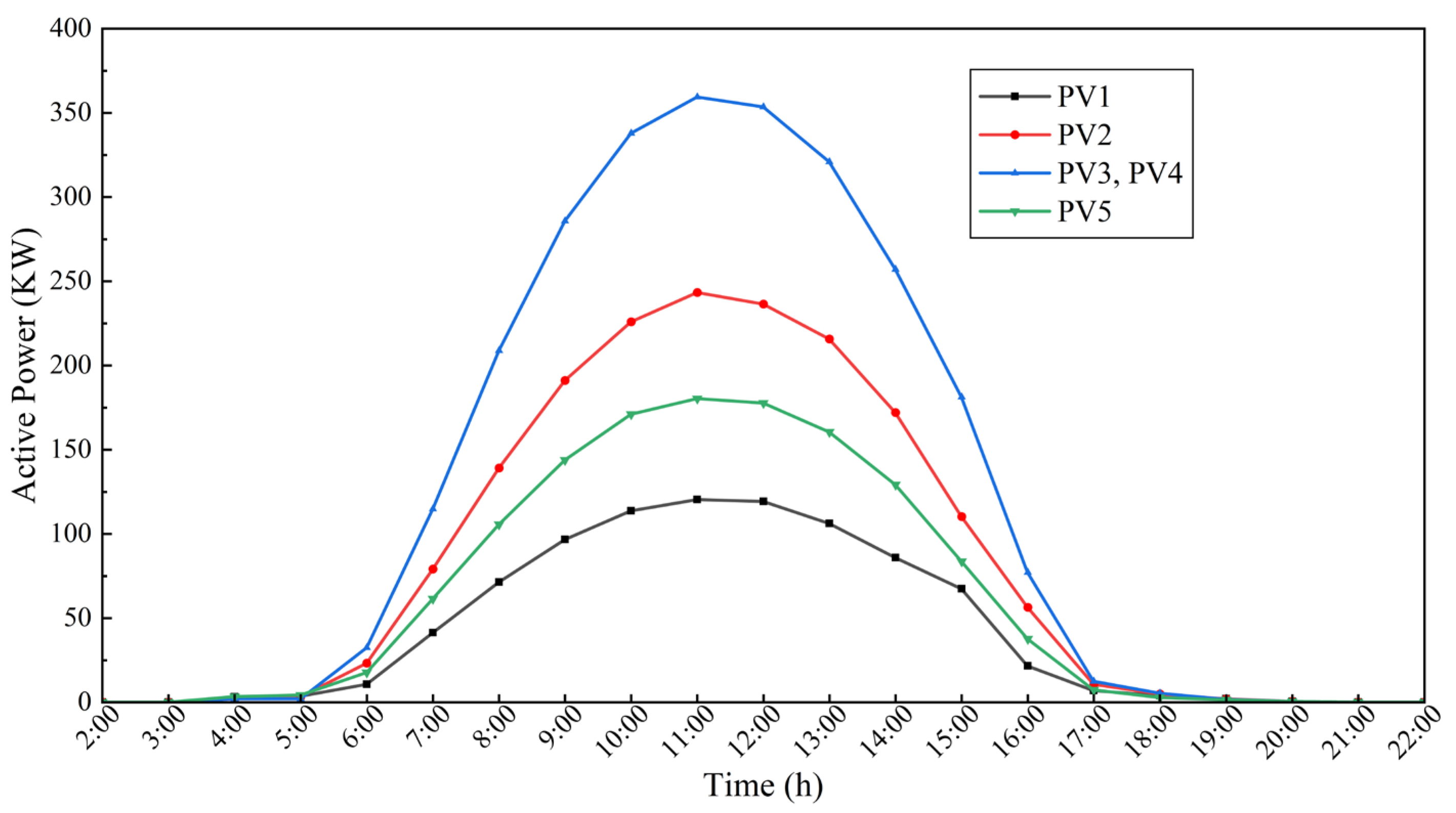
In Table 5, to encourage participation, a standard subsidy of 500 CNY per response is offered to qualifying EVCS that contribute to the emergency power supply. To account for the impact of V2G discharging on EV battery life, the unit degradation cost $c_{deg}$ is set to 0.6 CNY/kWh in the simulation, based on standard life-cycle energy throughput estimates. The active power output of the PV system is set to the day-ahead forecasted generation value, as shown in Figure 12.

Figure 12. Forecast output of PV units after disaster.

To assess computational performance, the hierarchical multi-stage emergency power supply model was coded in MATLAB 2021 using the YALMIP toolbox and solved with the GUROBI optimizer. The simulations ran on a desktop machine featuring an Intel Core i7 processor and 16 GB of memory.

3.2. Result Analysis

3.2.1. The Power Dispatching Potential of V2G-Enabled EVCS

This study establishes a V2G aggregator consisting of 200 EVs within a commercial district, with vehicle deployment aligned with typical daytime parking patterns. The charging behavior characteristics of various EV types, as detailed in Table 6, underpin the assessment of complex EV cluster charging demands. Vehicle parameters are derived from standard industry specifications, supplemented with stochastic variations to emulate real-world heterogeneity.

Table 6. The EV charging characteristics.

Vehicle Type	Charging Duration	Initial SOC	Battery Capacity (kWh)	Charging Modality	Arrival Time Distribution at Charging Stations
Private	09:00–17:00	50–70%	52.5–67.5	Slow charging (7 kW)	N * (9.0, 0.52) Commuting mode, concentrated network access during morning rush hour
Ride_hailing	off-peak hours (01:00–05:00, 10:00–16:00, 21:00–24:00)	15–30%	55–95	Fast charging (100–140 kW)	N * (3.0, 0.752), N * (13.0, 1.02), N * (22.5, 0.52)
Taxis	Morning shift: 06:00–08:00; Evening shift: 16:00–18:00	20–40%	55–85	Fast charging (40–60 kW)	N * (7.0, 0.332), N * (17.0, 0.422) Centralized network access for shift handover
Buses	Nighttime: 22:00–06:00; Daytime (minority): 12:00–14:00	30–50%	250–450	Fast charging (80–160 kW)	N * (0.0, 1.52), N * (13.0, 0.672) Primary access at night

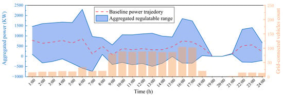
Private EV users mainly charge at commercial areas from 9:00 to 17:00, suitable for V2G participation. Ride-hailing vehicles charge opportunistically during off-peak hours: 1:00–5:00, 10:00–16:00, and 21:00–24:00. Taxis follow shift patterns, charging predominantly from 6:00–8:00 and 16:00–18:00. Approximately 80% of electric buses charge at night terminals, with 20% charging during the day (12:00–14:00). Using hybrid linear constraint modeling, an aggregation analysis on 200 EVs revealed the power regulation potential, illustrated in Figure 13, with the red dotted line for nominal power trajectory, blue area for adjustable range, and brown bars for connected vehicle counts per period.

Figure 13. Regulatable power region of V2G cluster.

The V2G-enabled EVCS exhibits maximal power regulation capacity between 09:00 and 17:00, reaching ±280 kW, attributed to private car grid integration. Power regulation fluctuates around 09:00 and 17:00 due to concentrated vehicle connection/disconnection. Midday regulation is reduced by vehicle usage and bus charging. Grid-connected vehicle numbers show a diurnal “dual-peak” in commercial areas: 09:00–10:00 (private cars and early taxi battery swaps) and 16:00–18:00 (late taxi swaps and private car grid connection). Night grid connection is minimal, primarily ride-hailing and buses. This differs from residential V2G clusters, which peak at night.

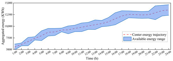
Figure 14 illustrates the EVCS’s aggregated electricity variation, with the red dotted line indicating benchmark power consumption and the blue shaded area denoting SOC feasible limits. Consumption initially rises due to simultaneous vehicle charging in the morning, then declines as V2G discharge begins and vehicles depart. The dispatchable electricity range initially is limited, expands during charging, and peaks mid-connection, constrained by EV physical limits: low initial SOC yields rigid demand; medium SOC allows flexible charging/discharging; approaching target SOC restricts discharge to prevent overcharging. At 17:00 off-grid, the range converges to meet return trip power requirements, reflecting travel demand constraints on V2G.

Figure 14. Feasible SOC region for the EV cluster.

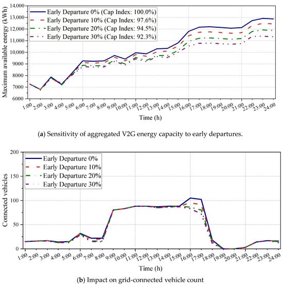
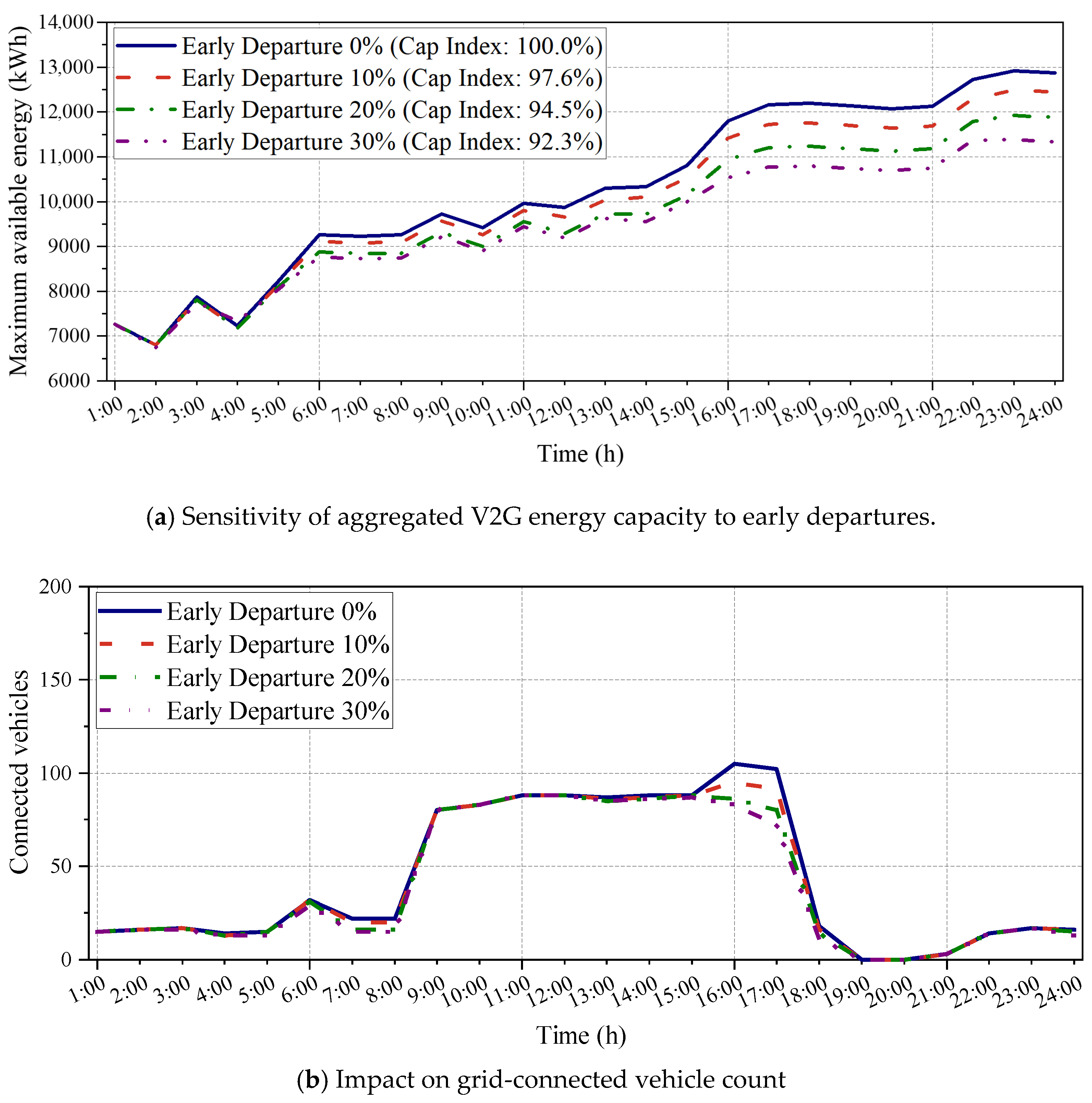
The baseline optimization constructs exact Minkowski sum boundaries assuming deterministic EV departure times. In real-world emergency scenarios, however, user behavior is rarely so predictable—early departures, for instance, can introduce significant uncertainty. To assess how such behavioral variability affects the aggregated V2G potential, we carried out a sensitivity analysis. Nested scenarios were simulated in which 10%, 20%, and 30% of EVs departed two hours earlier than scheduled.

Figure 15 captures the resulting spatiotemporal shifts. As the proportion of early departures rises, the number of grid-connected vehicles drops accordingly (Figure 15b). More critically, this uncertainty translates into a clear contraction of the aggregated virtual energy storage’s upper boundary, which becomes increasingly conservative as departure rates increase (Figure 15a). To quantify this effect, we computed the daily average of the maximum available energy, which is termed the V2G Capacity Index. Relative to the baseline, the index falls to 97.6%, 94.5%, and 92.3% under the 10%, 20%, and 30% early departure scenarios, respectively.

Figure 15. Sensitivity of the aggregated V2G potential to unexpected early departures.

These results highlight a useful feature of the proposed Minkowski aggregation framework: it remains sensitive to behavioral uncertainty and adapts accordingly. By contracting the feasible operational envelope ahead of dynamic scheduling, the model inherently prevents the grid from overestimating available emergency reserves. This, in turn, ensures that post-disaster dispatch commands remain physically feasible and reliably executable.

3.2.2. Pre-Disaster Selection Results

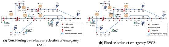
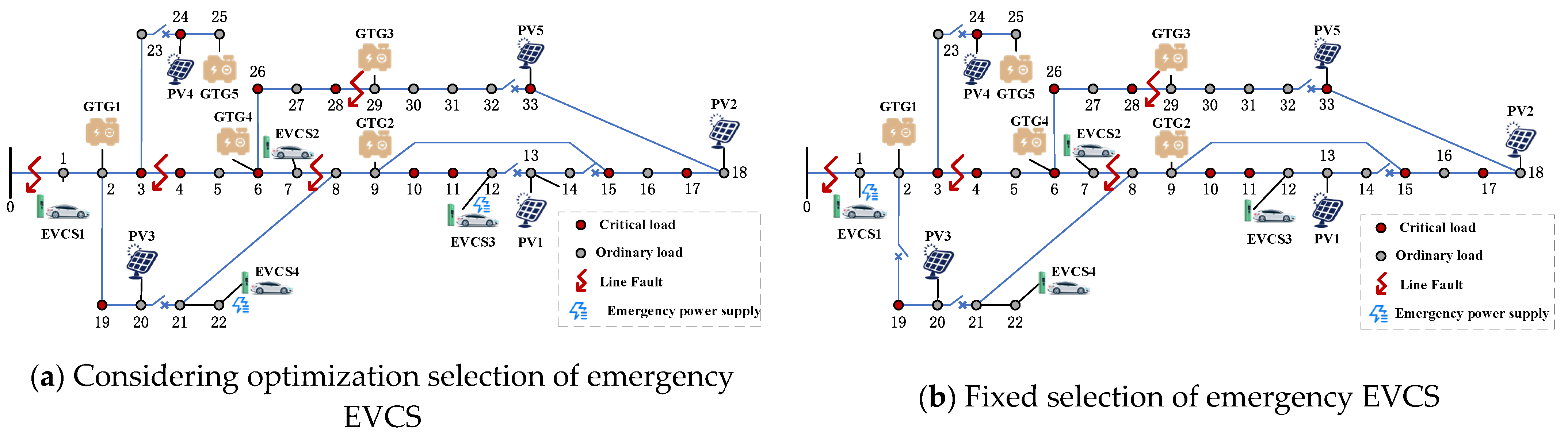
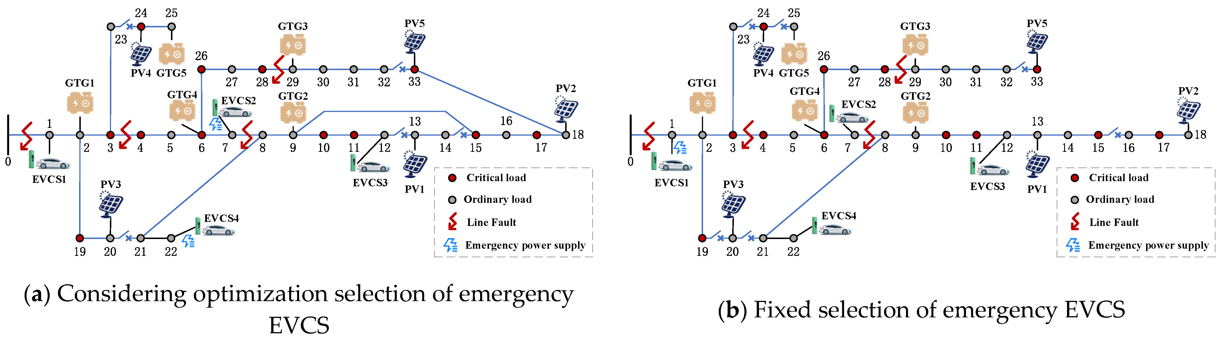
Under the condition that the PV output uncertainty $\tau$ is 0.35, the worst-case PV output in this study refers to the minimum reasonable output under extreme disaster scenarios, where the PV’s emergency power supply capacity is the weakest; accordingly, the deployment of electric vehicles and the participation cost of EVCS in emergency protection are relatively higher. The results of pre-selection of EVCSs and distribution network reconstruction are shown in Figure 16 and Figure 17. The pre-selection schemes prior to disaster are shown in Table 7. We introduce a comparative analysis based on deterministic optimization and robust optimization methods for a traditional fixed emergency power supply. The implementation methods of the comparative strategies can be found in [31,32], and have been adapted to the simulation scenario herein to ensure consistency in simulation parameters, system configurations, and evaluation metrics, thereby guaranteeing the fairness and reliability of the comparison results.

Figure 16. Deterministic optimization results.

Figure 17. Two-stage robust optimization results.

Table 7. Comparison of pre-selection schemes before disaster.

Scenario		Emergency Power Supply Selected	Optimize Selection Cost (CNY)	Load Reduction Cost (CNY)
Deterministic optimization	Considering optimization selection of emergency EVCS	EVCS3, EVCS4	1000	/
	Fixed selection of emergency EVCS	EVCS1	500	7665.9
	Fixed emergency power supply [31]	Node1	/	8597.6
Two-stage robust optimization	Considering optimization selection of emergency EVCS	EVCS2, EVCS4	1000	/
	Fixed selection of emergency EVCS	EVCS1	500	8085.7
	Fixed emergency power supply [32]	Node1	/	9173.8

Quantitative analysis in Table 7 indicates that fixed selection strategies, whether from deterministic optimization or integrated into the proposed robust framework, are limited by static resource allocation at predetermined nodes, with initial costs of approximately 500 CNY for EVCS and zero for emergency power supply. These static placements inflate operational load reduction costs to 7665.9 CNY and 8085.7 CNY for EVCS, and 8597.6 CNY and 9173.8 CNY, respectively, for emergency power. This reflects poor adaptability to uncertainties in fault duration, evolution, and PV output, compromising grid resilience. Conversely, the optimized EVCS selection within both frameworks employs flexible, cost-controlled deployment, effectively matching grid fault characteristics and optimizing V2G potential. The two-stage robust optimization outperforms deterministic methods by selecting EVCS2 and EVCS4, spatially aligned with critical nodes, and comprehensively addressing worst-case fault and PV variability scenarios. Unlike chance-constrained approaches, it does not require precise probability models, suitable for data-scarce disaster contexts. It also achieves joint optimization of EVCS placement and network topology, leveraging spatial and uncertainty synergies. Although load reduction costs are marginally higher than deterministic approaches, this trade-off enhances grid robustness against extreme events.

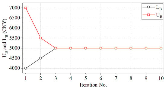
Figure 18 illustrates the convergence performance of the C&CG algorithm for the proposed two-stage robust optimization under the worst-case PV output scenario. The upper bound U_B and lower bound L_B converge rapidly, achieving the predefined optimality gap of 10⁻⁴ within four iterations. The total computation time is approximately 56.2 s, indicating that the proposed framework scales efficiently for distribution network power regulation without imposing excessive computational burden.

Figure 18. The iteration curves of upper and lower bounds for the two-stage robust optimization model.

3.2.3. Post-Disaster Recovery Results

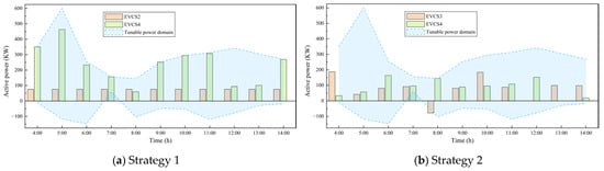
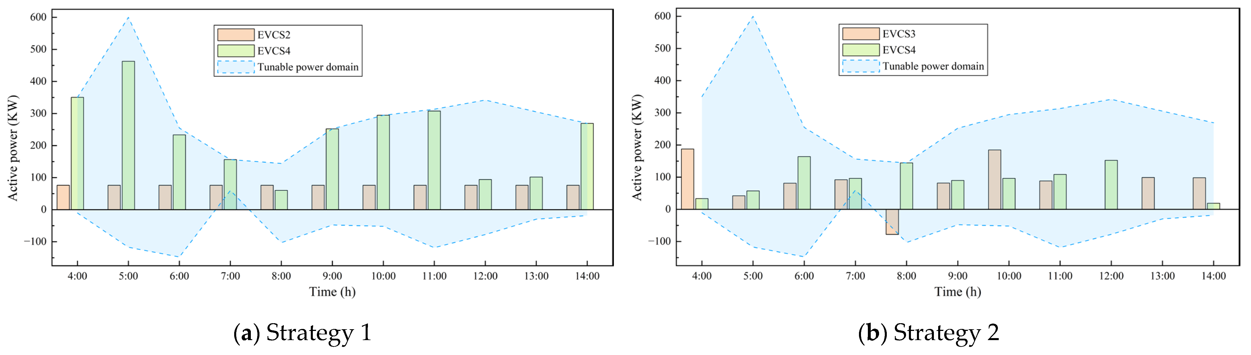
Following the disaster, numerous distributed energy resources actively coordinated their efforts to fully restore electrical load in affected regions. Figure 19 illustrates the real-time charging and discharging power and their corresponding power domains of EVCS under two strategic operational modes: Strategy 1 corresponds to pre-disaster robustness, while Strategy 2 corresponds to deterministic optimization. In practical dispatching, these stations effectively leverage the V2G potential inherent in electric vehicle networks. These charging stations not only play a critical role in enhancing grid resilience and efficiently restoring power supply but also provide essential support for grid stability during crises through their dynamic energy exchange capabilities, thereby significantly accelerating post-disaster recovery processes.

Figure 19. Charging and discharging power of EVCSs in each period.

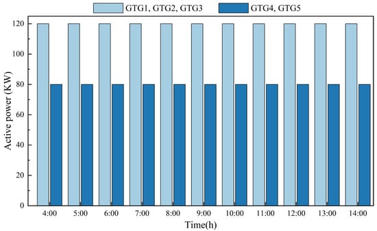
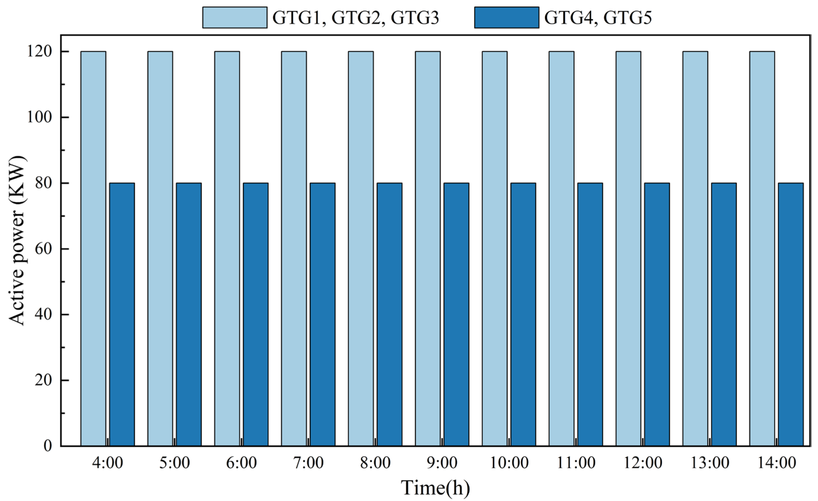
The output power of GTGs is illustrated in Figure 20, demonstrating the auxiliary power provision during the restoration phase.

Figure 20. Active power output of GTGs during post-disaster recovery.

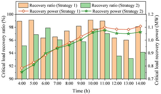
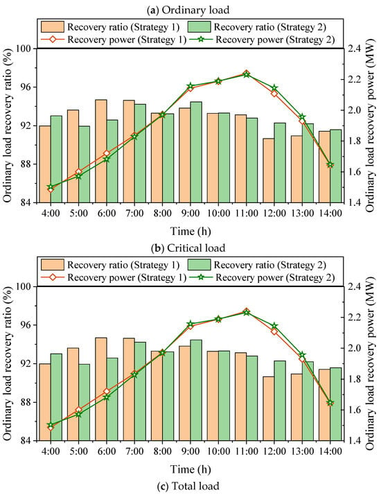
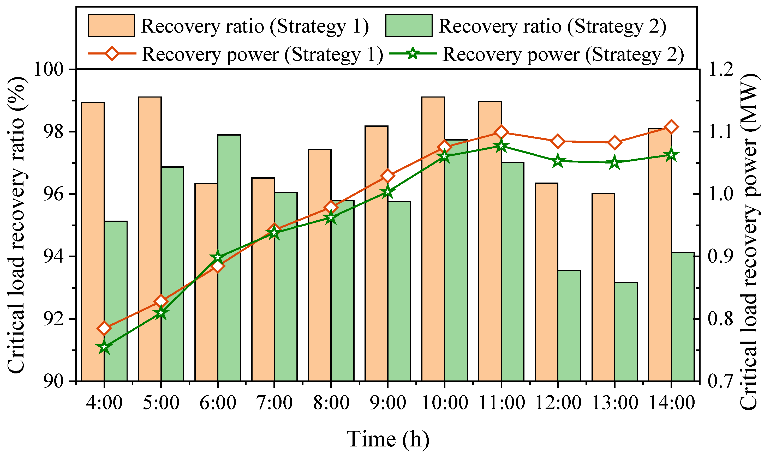
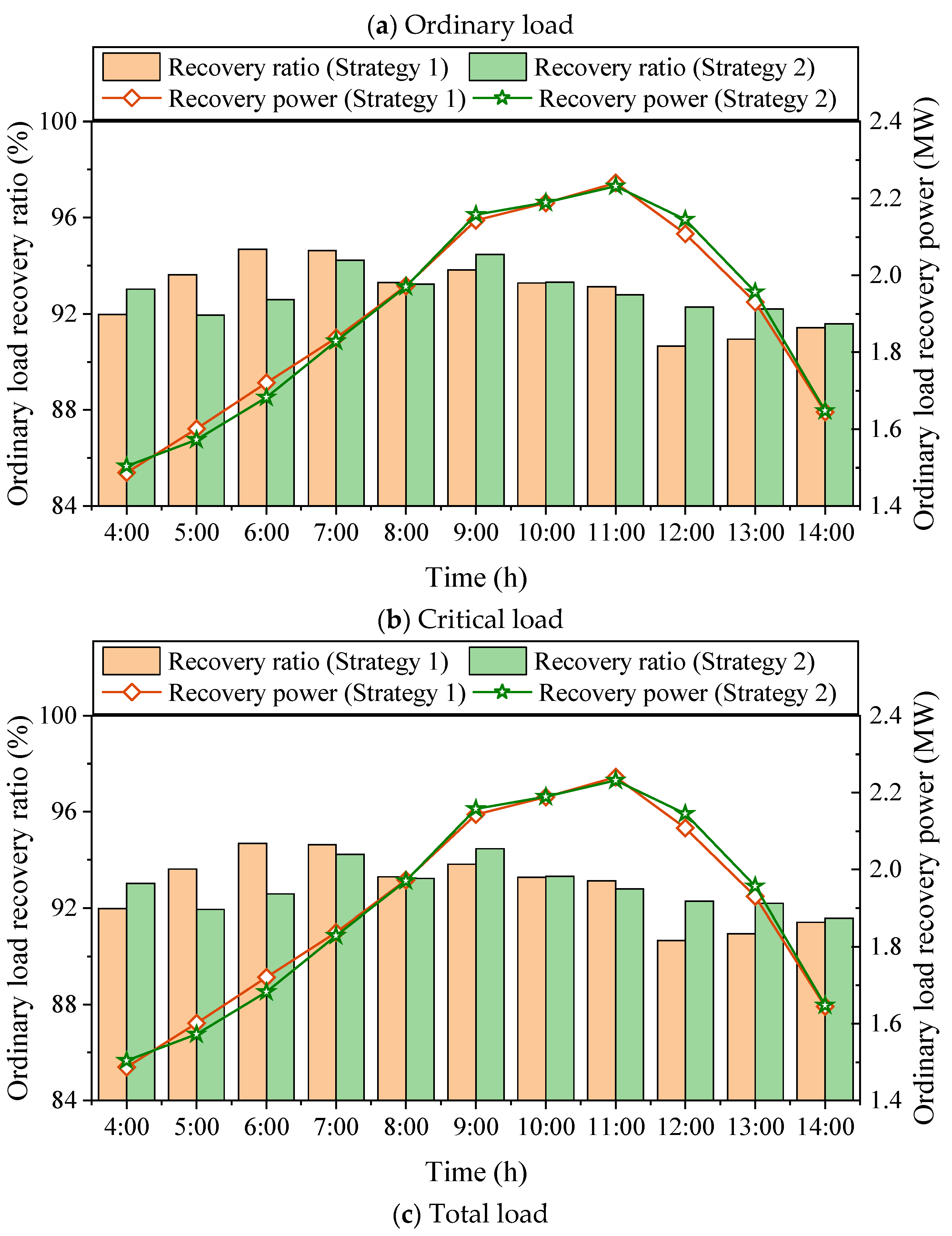
The recovery ratio and power of the two types of load in each period are shown in Figure 21.

Figure 21. Load recovery ratio and power at each time period.

As illustrated in Figure 21, the selection strategy for emergency EVCSs has a significant impact on load restoration effectiveness within the power grid. Specifically, Strategy 1 demonstrates a clear advantage over Strategy 2 in terms of load recovery performance. Quantitatively, Strategy 1 achieves a total load reduction power of 1.43 MW, with a corresponding load reduction cost of 37,639.59 CNY, and an average restoration ratio of critical loads reaching 97.7%. In contrast, Strategy 2 results in an increased total load reduction power of 1.63 MW and a higher load reduction cost of 57,437.22 CNY, while the average restoration ratio of critical loads slightly decreases to 95.7%. Despite both strategies maintaining an average restoration ratio of normal loads at 92.9%, the critical load recovery curves indicate that Strategy 1 consistently sustains higher restoration rates across most time periods. EVCS output analysis shows that Strategy 1 attains a net V2G power output of 3.42 MW, substantially exceeding Strategy 2′s 1.83 MW. This suggests that the EVCS selected under Strategy 1 more effectively leverages the V2G potential, resulting in higher power utilization and confirming that the choice of emergency charging stations plays a pivotal role in optimizing multi-source coordinated dispatch after disasters.

3.2.4. Scalability Validation

To evaluate the scalability and computational efficiency of the proposed two-stage robust optimization framework, further simulations were conducted on the modified IEEE 123-bus distribution system. The 123-bus network makes the resulting MILP significantly larger than the 33-bus system, which makes both the master problem and the subproblems in the C&CG solution algorithm much more complicated.

Table 8 shows that moving from the 33-bus system to the 123-bus system greatly increases the number of decision variables and constraints. The C&CG algorithm still reliably converges to the predefined optimality gap of 10^–4 within seven iterations, even though the scale has grown. The total computation time is about 452.6 s. Because decisions about which EVCS to select are usually made hours or days before an extreme weather event, a solution time of a few minutes is very realistic for engineering projects in the real world. These results show that the proposed framework, paired with efficient commercial solvers, can handle plenty of data and is an appropriate option for application in large-scale active distribution networks.

Table 8. Computational performance comparison.

Test System	No. of Nodes	MILP Variables	Iterations to Converge	Computation Time (s)	Optimality Gap
IEEE 33-bus distribution network	33	2124	4	56.2	10 × 104
IEEE 123-bus distribution network	123	18526	7	452.6	10 × 104

4. Conclusions

This paper proposes a pre- and post-disaster collaborative resilience enhancement strategy based on V2G interaction to address the issue of emergency power supply assurance in distribution networks during extreme disaster conditions. The results of the simulation demonstrate that this approach is effective, which leads to the following conclusions:

(1)

A refined model that takes into account two limits on power and energy boundaries was created to quantitatively describe the V2G regulation capacity of each EV. This model separates two main scenarios based on the SOC: one where it is below the acceptable minimum and one where it is above it. It then sets explicit constraints for each controllable domain and determines the best approaches for determining EV regulation capacity in each case. This lays the groundwork for combining the regulatory potential of EV clusters. To solve the problem of accurately characterizing EVCS regulation potential in real time, Minkowski sum theory was used to create a rolling optimization control framework. This framework makes it possible to aggregate EVCS power and energy feasible regions in real time and make dynamic updates to them. The results show that commercial-area EV clusters can reliably provide about ±300 kW of power regulation during peak daytime demand. However, there are significant variations in spatial and temporal distribution, which are important factors to keep in mind when planning and deploying EVs in the future.

(2)

To deal with the high level of uncertainty that originates with PV distributed generation output, a two-stage robust optimization model was developed during the phase of disaster prevention. This model discovers the most suitable locations for emergency EVCSs and daily distribution network operation strategies at the same time, cutting down on both the costs of deploying EVCSs and the costs of load shedding. It strictly limits the radial operation mode of the distribution network, the maximum output of the PV system, and the acceptable ranges of voltage fluctuations, which are all based on real-world engineering limits. A C&CG algorithm works well to solve the model. The results show that the proposed two-stage robust model slightly raises the initial investment for deploying EVs compared to traditional deterministic optimization models. However, it effectively reduces the effects of worst-case PV output uncertainty, which lowers the total costs of pre-disaster deployment and load loss in extreme conditions. This makes the distribution network more resilient to severe disruptions and strikes a balance between economic efficiency and robustness.

(3)

During the recovery from a disaster, a collaborative dynamic restoration model that combined different emergency resources like EVCS, GTGs, and PV was created. The model’s main goal is to reduce the weighted load shedding of the distribution network. Some of the main limits are the regulation ranges of distributed generation outputs and the operational limits after a fault. To make the model more useful and faster to compute, nonlinear constraints are turned into mixed-integer linear programming formulations. Simulation tests show that this multi-source collaborative model makes it possible to schedule emergency resources accurately, keeping key load restoration rates above 85% and the overall load recovery rate as high as 91.8%. A comparative analysis shows that the two-stage robust optimized EVCS deployment significantly improves V2G power output, lowers load shedding power and costs, and raises the average recovery rate of critical loads to 97.7% compared to deterministic EVCS deployment strategies. These changes make recovery times much shorter and make emergency power supply more reliable during disaster response.

(4)

To take battery degradation into account, the proposed model includes a linearized degradation cost penalty during dynamic scheduling to prevent excessive cycling. Because extreme distribution network faults are rare but have a big effect, the battery aging that happens when you respond to disasters over and over again is not very significant. Even so, it is still important to include this degradation as an economic compensation cost in the objective function in order to encourage EV owners to participate and keep the V2G scheme relevant in the real world.

Future research seeks to enhance the existing applied modeling methodology with significant theoretical advancements by concentrating on theoretical abstraction, methodological generalization, and cross-domain integration. The fundamental principle of “pre-disaster robust planning and post-disaster dynamic recovery” inherent in the V2G resilience strategy will be distilled into a universal “spatiotemporal resilience coordination theory” for distributed flexible resources, clarifying the interconnections among temporal flexibility, spatial distribution, and resource complementarity, irrespective of particular contexts. The Minkowski summation-based dynamic potential aggregation method will be expanded into a comprehensive heterogeneous resource aggregation theory, incorporating derived bounds and error quantification to rectify the deficiency of cohesive theoretical direction. Coupled assessment indices and co-optimization frameworks will be used to model interactions between transportation (EV behavior) and distribution networks (resilience needs) across domains. These frameworks will use advanced methods for handling uncertainty to deal with changing fault locations and random EV user behavior, and they will also include low-carbon goals to align resilience with energy transition goals. These developments will fortify the theoretical framework, broaden research avenues, and augment the academic and practical impact of power system resilience studies.

References

- Ma, S.; Chen, B.; Wang, Z. Resilience Enhancement Strategy for Distribution Systems under Extreme Weather Events. IEEE Trans. Smart Grid 2018, 9, 1442–1451. [Google Scholar] [CrossRef] [Scilit]
- Bie, Z.; Lin, Y.; Li, G.; Li, F. Battling the Extreme: A Study on the Power System Resilience. Proc. IEEE 2017, 105, 1257–1273. [Google Scholar] [CrossRef] [Scilit]
- Cao, Y.; Cui, J.; Liu, S.; Li, X.; Zhou, Q.; Hu, C.; Liu, Z. A Holistic Review on E-Mobility Service Optimization: Challenges, Recent Progress, and Future Directions. IEEE Trans. Transp. Electrif. 2023, 10, 3712–3741. [Google Scholar] [CrossRef] [Scilit]
- Rahimi, K.; Davoudi, M. Electric Vehicles for Improving Resilience of Distribution Systems. Sustain. Cities Soc. 2018, 36, 246–256. [Google Scholar] [CrossRef] [Scilit]
- Ahmed, F.; Ahmad, S.; Rahman, M.T.; Hazari, M.R.; Faiz, R.; Ahmed, T.; Karimi, M. A holistic review of electric vehicle charging impacts on power distribution networks: Technical challenges, smart mitigation strategies and future directions. Appl. Energy 2026, 402, 126961. [Google Scholar] [CrossRef] [Scilit]
- Wang, J.; Zhao, Y.; Li, H.; Xu, X. Enhanced photovoltaic-powered distribution network resilience aided by electric vehicle emergency response with willingness and reward. Appl. Energy 2025, 389, 125619. [Google Scholar] [CrossRef] [Scilit]
- Dong, Q.; Zhou, G.; Huang, Q.; Dong, Z.; Jia, Y. Resilience enhancement for power distribution networks in coordination with electric vehicle fleets. Appl. Energy 2025, 390, 125756. [Google Scholar] [CrossRef] [Scilit]
- Zhang, X.; Liu, Y.; Wang, Z.; Chen, H.; Li, J. Urban Grid Resilience Assessment Framework: Leveraging Electric Vehicles, Time-Based Analysis, and Mobile Distributed Generators for Repair Crew Strategic Deployment. Sustain. Energy Grids Netw. 2025, 41, 101588. [Google Scholar]
- Wang, Y.; Zhang, N.; Kang, C.; Miao, M.; Shi, R.; Xia, Q. An Efficient Approach to Power System Uncertainty Analysis with High-Dimensional Dependencies. IEEE Trans. Power Syst. 2018, 33, 2984–2994. [Google Scholar] [CrossRef] [Scilit]
- Dong, J.; Liu, C.; Lin, Z. Charging Infrastructure Planning for Promoting Battery Electric Vehicles: An Activity-Based Approach Using Day-to-Day Travel Data. Transp. Res. C Emerg. Technol. 2014, 38, 44–55. [Google Scholar] [CrossRef] [Scilit]
- Mei, H.; Wu, Q.; Ren, H.; Zhang, J.; Li, Q. Optimization of electric vehicle charging station layout considering the improvement of distribution network resilience under extreme disasters. Energy 2025, 323, 135831. [Google Scholar] [CrossRef] [Scilit]
- Hao, J.; Huang, T.; Xu, Q.; Sun, Y. Robust Optimal Scheduling of Microgrid with Electric Vehicles Based on Stackelberg Game. Sustainability 2023, 15, 16682. [Google Scholar] [CrossRef] [Scilit]
- Wang, D.; Gao, H.; Chen, Y.; Zhang, B.; Sun, Q. Resilience Enhancement Strategies for and Through Electric Vehicles. Sustain. Cities Soc. 2022, 80, 103788. [Google Scholar] [CrossRef] [Scilit]
- Zou, X.; Wang, Y.; Strbac, G. A resilience-oriented pre-positioning approach for electric vehicle routing and scheduling in coupled energy and transport sectors. Sustain. Energy Grids Netw. 2024, 39, 101484. [Google Scholar] [CrossRef] [Scilit]
- Ghasemi, S.; Moshtagh, J. Distribution system restoration after extreme events considering distributed generators and static energy storage systems with mobile energy storage systems dispatch in transportation systems. Appl. Energy 2022, 310, 118507. [Google Scholar] [CrossRef] [Scilit]
- Shen, Y.; Qian, T.; Li, W.; Zhao, W.; Tang, W.; Chen, X.; Yu, Z. Mobile energy storage systems with spatial–temporal flexibility for post-disaster recovery of power distribution systems: A bilevel optimization approach. Energy 2023, 282, 128300. [Google Scholar] [CrossRef] [Scilit]
- Zheng, C.; Chen, F.; Xi, Z.; Guo, G.; Yang, X.; Chen, C. A Resilience Entropy-Based Framework for V2G Charging Station Siting and Resilient Reconfiguration of Power Distribution Networks Under Disasters. World Electr. Veh. J. 2025, 16, 532. [Google Scholar] [CrossRef] [Scilit]
- Shi, Y.; Zhou, C.; Zhang, C.; Ma, Y.; Zhang, M.; Chen, Z.; Liu, X.; Huang, Q. Enhancing Power System Resilience: A Comprehensive Approach Utilizing Electric Vehicles and Dynamic Microgrids. Comput. Ind. Eng. 2026, 212, 111664. [Google Scholar] [CrossRef] [Scilit]
- Refaat, M.M.; Al-Dhaifallah, M.; Ismail, M.M.; AbouOmar, M.S.; El Ferik, S. Dimensionality-reduced multi-objective framework for resilient power systems with electric vehicles and hydrogen-based energy storage. Sci. Rep. 2025, 15, 45150. [Google Scholar] [CrossRef] [Scilit]
- Yin, D.; Ouyang, J.; Li, A.; Wang, J.; Zhao, X. Adaptive fault ride-through control method for V2G charging stations with voltage support capability. Power Syst. Prot. Control 2026, 54, 116–126. [Google Scholar]
- Dong, Z.; Zhang, X.; Kang, C.; Strbac, G. A Distributed Robust Control Strategy for Electric Vehicles to Enhance Resilience in Urban Energy Systems. Appl. Energy 2022, 316, 119042. [Google Scholar] [CrossRef] [Scilit]
- Panda, N.K.; Tindemans, S.H. Efficient Quantification and Representation of Aggregate Flexibility in Electric Vehicles. Electr. Power Syst. Res. 2024, 213, 110811. [Google Scholar] [CrossRef] [Scilit]
- Zhang, S.; Zhang, C.; Long, Z. Orderly charging and discharging dispatching strategy for electric vehicles based on microgrid. Energy 2025, 340, 139054. [Google Scholar] [CrossRef] [Scilit]
- Zou, H.; Gao, W.; Zhang, Y.; Xia, J.; Liu, Z. Polytope-Based Flexible Aggregation and Disaggregation Strategy for Electric Vehicles. In Proceedings of the 2025 IEEE International Conference on Industrial Technology (ICIT), Wuhan, China, 26–28 March 2025; pp. 1–7. [Google Scholar]
- Yang, M.; Wang, H.; Zhao, Y.; Sun, P.; Ge, J. Day-ahead distributed robust scheduling of active distribution networks considering source-load uncertainties and large-scale electric vehicle integration. Int. J. Electr. Power Energy Syst. 2025, 163, 111429. [Google Scholar] [CrossRef] [Scilit]
- Wang, H.; Fang, Y.-P.; Zio, E. Resilience-Oriented Optimal Post-Disruption Reconfiguration for Coupled Traffic-Power Systems. Reliab. Eng. Syst. Saf. 2022, 222, 108408. [Google Scholar] [CrossRef] [Scilit]
- Du, Y.; Zhang, J.; Chen, Y.; Liu, Z.; Zhang, H.; Ji, H.; Wang, C.; Yan, J. Impact of electric vehicles on post-disaster power supply restoration of urban distribution systems: A spatio-temporal coupling approach. Appl. Energy 2025, 325, 125302. [Google Scholar] [CrossRef] [Scilit]
- Liu, Y.; Zhang, H.; Wang, J.; Li, X. Research on the Coordinated Recovery Strategy Based on Centralized Electric Vehicle Charging Station. Energies 2023, 16, 5401. [Google Scholar] [CrossRef] [Scilit]
- Churchill, M.; Monroe, J.; Bristow, D.; Crawford, C. Using electric vehicles to enhance power outage resilience—An agent-based modeling approach. Heliyon 2024, 10, e32104. [Google Scholar] [CrossRef] [Scilit] [PubMed]
- Xu, X.; Qiu, Z.; Zhang, T.; Gao, H. Distributed Source-Load-Storage Cooperative Low-Carbon Scheduling Strategy Considering Vehicle-to-Grid Aggregators. J. Mod. Power Syst. Clean Energy 2024, 12, 440–453. [Google Scholar] [CrossRef] [Scilit]
- Han, C.; Liang, B.; Lin, Z.; Wen, F.; Yi, S. Chance-Constrained Programming Method for Optimal Scheduling of Emergency Power Source. Electr. Power Autom. Equip. 2018, 38, 147–154. [Google Scholar]
- Wang, Z.; Sun, L.; Lin, Z.; Wen, F.; Yi, S.; Zhang, H. Optimal Allocation of Emergency Power Sources Considering Uncertainties of Loads and Dispatching Time Periods. Autom. Electr. Power Syst. 2018, 42, 34–41. [Google Scholar]
Disclaimer/Publisher’s Note: The statements, opinions and data contained in all publications are solely those of the individual author(s) and contributor(s) and not of MDPI and/or the editor(s). MDPI and/or the editor(s) disclaim responsibility for any injury to people or property resulting from any ideas, methods, instructions or products referred to in the content. |
© 2026 by the authors. Licensee MDPI, Basel, Switzerland. This article is an open access article distributed under the terms and conditions of the Creative Commons Attribution (CC BY) license.