Neural Network Auto-Design Algorithm for Urban Travel Time Prediction

Abstract

This paper proposes to estimate the travel time at each edge of an urban street network using Artificial Neural Networks (ANNs). To improve the ANN performance and minimize errors in manual design, an Algorithm Auto-Design ANN Topology (A-DANNT) is introduced that automatically determines the most suitable architecture for regression problems. The methodology implements an algorithm based on Tabu Search, called the Best R-Value Determination algorithm (BR-vD), which optimizes the topology obtaining a lower Mean Square Error (MSE) and a higher correlation coefficient. The process is developed in three phases: first, the variables that impact the travel time are analyzed; then, the proposed algorithm is used to find the best topology; and finally, the travel times are estimated. The proposal is evaluated in two case studies: in the first, the algorithm automatically designs the architecture, and a 0.99366 correlation coefficient is achieved between the results and the objectives. In the second case, the performance of the algorithm is compared with a fuzzy travel time model, achieving a 0.99898 correlation coefficient. In both cases, the proposed algorithm is capable of designing topologies with coefficients greater than 0.99 and Mean Absolute Errors (MAEs) of 3.2765 and 0.6957 s, respectively.

1. Introduction

Companies engaged in distributing goods or needing to send their product to a specific point and offer deliveries on the same day or on a limited schedule face problems of delayed deliveries and high operating costs [1]; likewise, customers increasingly demand better service and timely deliveries [2]. The demand for orders causes drivers to also travel through different streets in poor conditions and sometimes in the presence of rain. On the other hand, home delivery is growing and could become an attractive market for urban logistics providers due to the growing internet shopping boom. In addition, derived from the confinement caused by the COVID-19 pandemic to avoid contagion in shopping centers and markets [3], there has been an increase in demand for orders, online purchases, and home deliveries [4]. Furthermore, demand is growing mainly on digital food platforms and first-need-use purchases [5]; home service has become critical, and e-commerce purchases have grown and could prevail as habits even after the end of compulsory confinement, which makes it necessary for companies to ensure timely deliveries and delivery policies.

The best route optimization solutions help home delivery companies minimize drive time, ensure timely product delivery, and lower operating costs [6,7]. In addition, they help obtain the benefits of reducing fuel consumption and emissions of gases that are harmful to the environment [8]; in the same way, they reduce the maintenance and excessive vehicle expenses caused by wear and tear and travel along routes in poor conditions.

The objective of predicting travel time is to know in advance how long it takes to go from one node to another without having started the journey; thus, the user (delivery driver, transport driver, bus driver, traveler) or anyone who needs to move can reduce waiting times or late arrivals [9,10,11,12,13].

Some areas use travel time and traffic information to choose better routes and ensure arrival time: planning transport networks [14,15], public transport [16], and intelligent transport [17,18,19,20]. Its use becomes practical when it is necessary to predict bus travel times from the source to the stops [11,21], mainly in public transport applications within the city or on highways and freeways [13,22], but even in the private sector in transport and logistics planning [23].

The literature frames two types of methods for estimating trip times, model-based methods and data-based methods [9,10,24]. Model-based methods explore and analyze the relationship between traffic variables and physical variables [25]. Data-driven models estimate travel times based on historical data for certain factors [26,27,28,29,30,31,32].

Forecasting travel times on urban roads becomes difficult due to the uncertainty it presents and the stochastic nature of different factors that constantly affect and modify travel times, making it challenging to predict travel times with traditional models [33,34], creating a need to analyze the variables that describe the system’s behavior to ensure good prediction. To model uncertainty in [35], it is considered a random variable, or in [36], where the weights of each edge are present randomly. Other authors integrate probabilistic elements into mathematical models to model uncertainty; however, this increases its complexity to solve it [24,37,38,39]. Some works use Bayesian neural networks to predict stochastic travel times in urban networks [37,38]. In [39], to predict travel time’s probability distribution on routes, the author uses random values, and a TRIP method collects GPS data from mobile phones. Zhenliang’s work focuses on estimating the probability distribution of travel times from time distributions using Markov chains, proposing heuristic clustering methods for observations and traffic conditions [24].

The literature uses the term travel time reliability as the relationship between the travel time value variability and the travel time value [40]. Ref. [40] proposes a method of estimating the distribution of travel times by applying the travel time reliability ratio (TTRR) and the conditional value at risk (CVaR). Ref. [41] examines the factors that impact travel time on health care accessibility, proposes a reliability-based 2SFCA method, and obtains a dataset of taxi trajectories to extract information on time distributions.

Ref. [42] focuses on obtaining the total monetary cost of travel time and the transit rate in Chicago public transport; also, the authors measure travel time in a magnitude, transit fare, and revenue into one unit, considering the total monetary cost of the trip as a revenue percentage.

The data provides accurate and valuable information in travel time prediction; likewise, the accuracy increases with current value data collection [12,25,43]. In works such as those of [10], the data is obtained through applied surveys using historical data and statistical methods. In [44], the authors determine travel times with statistical methods of machine learning, linear regression, neural networks, regression trees, nearest k-neighbors, and locally weighted regression; in the end, the authors compare the results obtained on the same historical data.

Data-based models and solutions depend on the dataset supply. In [28], the author applies Support Vector Regression (SVR) using accurate road traffic data for travel time prediction. In [45], the authors use GPS data and the Kalman filter technique to predict travel times in arteries where special events cause a sudden increase in traffic.

A road network, with many nodes and edges estimated, is simple to process for today’s computers; however, it is necessary to assess uncertainty using heuristic methods that facilitate data processing time and assess factors affecting travel time [46]. Neural networks have been beneficial when evaluating a large amount of information [31,32,47].

In [26], Modular Neural Networks are used for real-time travel time prediction on highways in San Antonio, Texas. The information is collected by sensors installed along the motorway, connected to a network of high-speed computers and GPS systems. In [27], the authors present a network of counterpropagation (CPN) to forecast travel time on highways, comparing their topology with backpropagation training. In [29], the authors propose to use Parallel Microscopic Simulation (PARAMICS) to simulate computer data from a transport network; simulated data is used to train a neural network. In [30], the authors use recurrent neural networks, specifically State-Space Neural Networks (SSNNs), to predict travel times on highways using synthetic data. Recent works such as those of [48] propose algorithms based on deep learning to predict travel time, use temporary space analysis and pattern recognition and an external database, apply a methodology with a series of steps, perform data cleaning, detect outliers, perform data augmentation, feature extraction, feature representation, and finally,  prediction.

At present, Artificial Neural Network applications are mainly used to predict behaviors of complex systems. Both performance and computational complexity depend largely on variables and the datasets that relate to the problem and describe the system’s behavior. Likewise, the neural network configuration must be composed of layers, neurons, synaptic weight, and activation functions, commonly called hyperparameters [49]. For regression problems, the network design is based on the developer’s experience, and its architecture is designed arbitrarily or through trial and error [50,51,52]. In another case, it is necessary to search for alternatives for the architecture design, avoiding configuring its topology manually [53], making it cumbersome and laborious to choose and change the configuration until obtaining an architecture that guarantees a favorable and almost optimal result. Similarly, in an Artificial Neural Network, obtaining the optimal initial weights that guarantee the best results or are very close to the best is necessary.

This work focuses on obtaining the travel times for each edge of the network with training of the neural network using factors that affect the travel time with historic data and do not focus on obtaining the reliability of the travel times. Each of the factors analyzed in this work directly affects travel times and changes over time, resulting in significant changes and the updating of factors that directly affect travel time. Likewise, the input variables are considered dynamic over time and constantly changing state, causing the weighting of the factors to be constantly updated.

This work proposes to estimate the travel time for all edges in an urban street network by proposing an A-DANNT algorithm and a Tabu Search-based algorithm called BR-vD in order to determine the architecture that best adapts to the input values and the output data, obtaining the lowest MSE and the best correlation coefficient. This article considers the factors that affect the delivery process in a food delivery company, selecting the factors that present a greater degree of occurrence and impact on delivery time. The model accurately estimates values from a dataset.

The methodology is divided into three stages; the first involves obtaining the dataset: street status (Ss), traffic zone (Tz), rainfall (Rl), time of the day (Td), Street distance (Sd). In the second stage, the appropriate topology is selected with the help of a proposed A-DANNT algorithm. Based on the heuristic Tabu Search, the number of neurons and the number of the layers are selected sequentially, evaluating combinations of neurons, the choice, and design. The algorithm’s sequential search provides a better correlation coefficient and eventually stops the process if it does not improve the result, thus avoiding unnecessary training times. The proposed algorithm evaluates and chooses the number of layers and the number of neurons needed for each case, improving the estimation of travel times and minimizing the choice error, obtaining an appropriate configuration and topology with a lower MSE and the best correlation coefficient. The third stage estimates the travel times for each edge of the network; this stage is performed each time the user requires it.

The proposed A-DANNT framework differs from conventional Neural Architecture Search approaches in both objective and search scope. Instead of exploring large continuous architecture spaces, the method performs a constrained discrete exploration over the number of layers and neurons using a Tabu-based memory mechanism to avoid redundant evaluations.

Moreover, the architecture selection criterion is based on statistical consistency of the predictions measured through the correlation coefficient, rather than solely minimizing residual error. Consequently, the method should be interpreted as a task-oriented topology adaptation strategy for regression problems rather than a general NAS optimization framework.

Urban road networks inherently exhibit structural symmetries, since multiple routes share similar geometric and traffic patterns such as equivalent distances, traffic density regimes, and temporal flow distributions. These symmetries generate invariances in the travel time prediction problem: different spatial configurations may produce statistically equivalent travel conditions.

The proposed A-DANNT model implicitly exploits these invariances by automatically adapting the network topology to the data distribution. Instead of learning route–specific behaviors, the model learns classes of equivalent traffic states, allowing generalization across symmetric traffic scenarios. Consequently, the predictive model operates over equivalence classes of traffic conditions rather than individual observations, establishing a direct connection between the proposed learning framework and symmetry-based modeling principles.

The proposed methodology and materials used in this article are mentioned in Section 2; two practical cases that demonstrate the effectiveness of the proposed algorithm are shown in Section 3; finally, the discussion and conclusions are presented in Section 4.

2. Materials and Methods

2.1. Neural Network

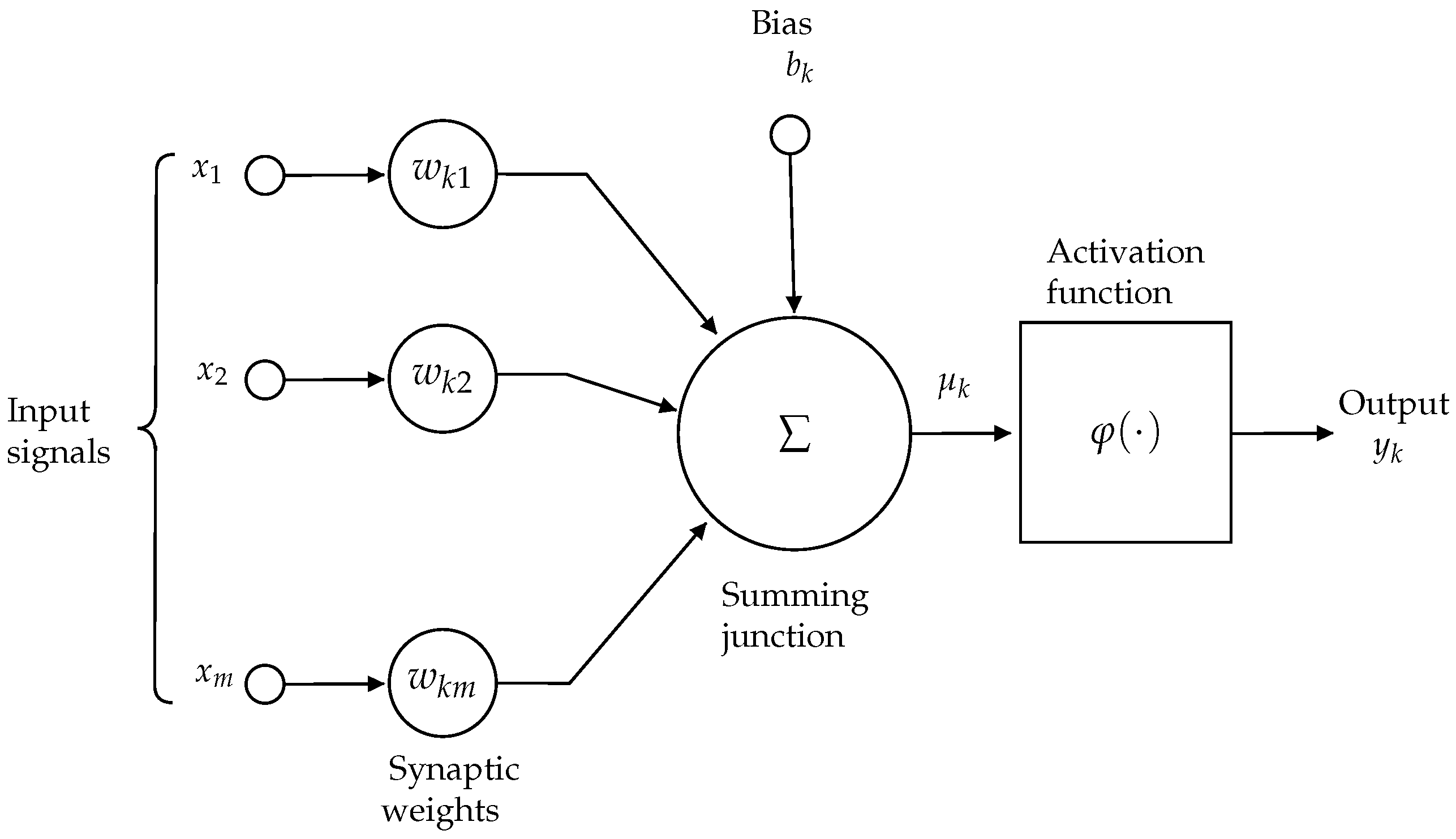
Generally, a biological neuron’s behavior is of a nonlinear type [54]; characteristic ANNs have a greater interest in different areas. Haykin [55] defines the neuron as an information processing unit, identifying three essential elements: (1) A set of inputs ($x_1,x_2,x_m$) with synaptic weights ($w_{k1},w_{k2},w_{km}$), representing the received signals; (2) an aggregation function, which combines these signals into a single net output (${\mu }_k$); and (3) a nonlinear activation function ($\phi \left({\mu }_k\right)$), which determines the final output of the neuron ($y_k$). This model allows ANNs to capture complex patterns and perform tasks such as classification, prediction, and pattern recognition (see Figure 1).

Figure 1. The neuron nonlinear model.

• A set of synapses, defined as an entry $x_j$ connected to a neuron k multiplied by a synaptic weight $w_{k,j}$.
• A summation input signal weighted by synaptic weights.
• Activation function to limit the amplitude of the output of a neuron.

The neural model is described in Equations (1) and (2):

$$\begin{array}{cc}\hfill {\mu }_k& =\sum _{j=1}^m{w}_{k,j}{x}_j+b_k\hfill \end{array}$$

(1)

$$\begin{array}{cc}\hfill y_k& =\phi \left({\mu }_k\right)\hfill \end{array}$$

(2)

where $x_1,x_2,\dots ,x_m$ are input signals; $w_{k,1},w_{k,2},\dots ,w_{k,m}$ are the synaptic neuron weights k; ${\mu }_k$ is the combination of input signals with synaptic weights, where $b_k$ is the bias term that shifts the activation threshold of the neuron rather than the output value; $\phi (·)$ is the activation function and $y_k$ is the output neuron signal. Several types of activation functions are used in neuron modeling.

In [54], the author describes three essential concepts within the structure of an ANN—computational parallelism, distributed memory, and environment adaptability—to adapt quickly and learn from experience. These three properties configure an Artificial Neural Network system, where the essential element is the artificial neuron, the connections between neurons form a layered pattern, and several layers create a neural network. The ANN architecture consists of the neural network, input variables that act as a data receiver, or input of external stimuli, output variables, and hyperparameters.

2.2. Training Methods

The ANN intends to imitate human brain processing, which leads to the learning process, so that an expected result is obtained; there are mainly two types of learning, one in memory or execution mode and the other in learning or training mode [54]. The learning feature is handy because of its ability to perform a given process by learning input and output patterns.

Backpropagation and Differentiation

It is a learning algorithm that seeks to minimize the error between the neural network’s output and the desired output value, optimizing the network weights and adjusting the values, applying a gradient descent. It is necessary to efficiently calculate partial derivatives of an approximate function $F(\mathbf{W},\mathbf{X})$ of the net concerning all elements of the vector of weight $\mathbf{W}$ for a given value of the vector of input $\mathbf{X}$.

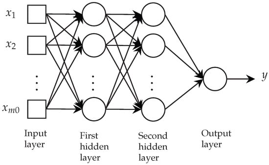
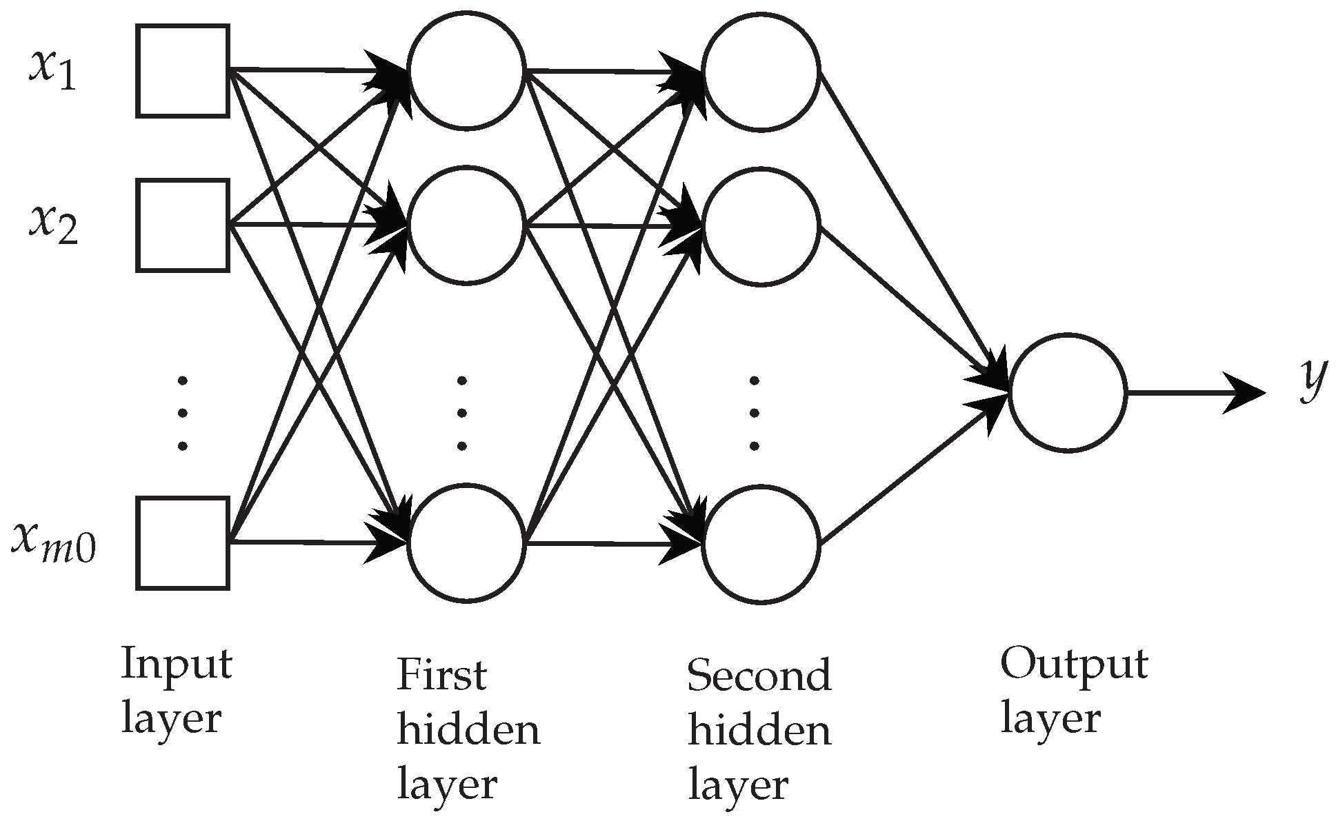
Ref. [55] considers a multilayer perceptron with an input layer of $m_0$ nodes, two hidden layers, and a single output neuron (see Figure 2), each with its respective $w{\left(l\right)}_{ji}$ considered as the neuron´s synaptic weight i to the neuron j in layer $l=1,2,3$, where $l=1$ corresponds to the first hidden layer of the network and $l=3$ belongs to the output layer. We want to evaluate the derivatives of the function $F(\mathbf{W},\mathbf{X})$ with respect to all elements of the vector weight $\mathbf{W}$ for a specified input vector $\mathbf{X}={[x_1,x_2,\dots ,x_{m_0}]}^T$. For example, for a network with $l=2$, it is described as

$$F(\mathbf{W},\mathbf{X})=\sum _{j=0}^{m_1}{w}_{o,j}\phi \left(\sum _{i=0}^{m_0}{w}_{ij}{x}_i\right)$$

(3)

where $\mathbf{W}$ is the weight vector and $\mathbf{X}$ is the input vector.

Figure 2. Multilayer perceptron with two hidden layers.

The multilayer perceptron in Figure 2 is parameterized by $\Lambda$ architecture (which represents a discrete parameter) and a weight vector w composed of continuous elements. Suppose that $\Lambda {\left(l\right)}_j$ denotes that part of the architecture that extends from the input layer ($l=0$) to the j node in layer $l=1,2,3$. Therefore,

$$F(\mathbf{W},\mathbf{X})=\phi \left({\Lambda }_1^{\left(3\right)}\right)$$

(4)

where, $\phi$ represents the activation function, and $\Lambda 3_1$ represents a symbol of architecture rather than a variable. Consequently, the gradient of the error function is computed using the standard backpropagation formulation.

For a multilayer perceptron, the derivative of the error function with respect to a weight is

$${\displaystyle \frac{\partial E}{\partial w_{ij}^{\left(l\right)}}}={\delta }_j^{\left(l\right)}{a}_i^{(l-1)}$$

(5)

where $a_i^{(l-1)}$ denotes the activation of neuron i in the previous layer and ${\delta }_j^{\left(l\right)}$ is the local error term of neuron j in layer l.

For the output layer,

$${\delta }_j^{\left(L\right)}=(y_j-t_j){\phi }^{\prime }\left(u_j^{\left(L\right)}\right)$$

(6)

For hidden layers,

$${\delta }_j^{\left(l\right)}={\phi }^{\prime }\left(u_j^{\left(l\right)}\right)\sum _k{w}_{jk}^{(l+1)}{\delta }_k^{(l+1)}$$

(7)

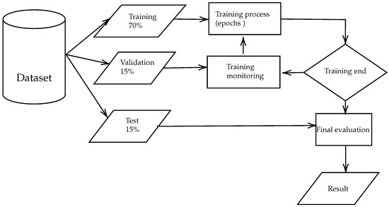
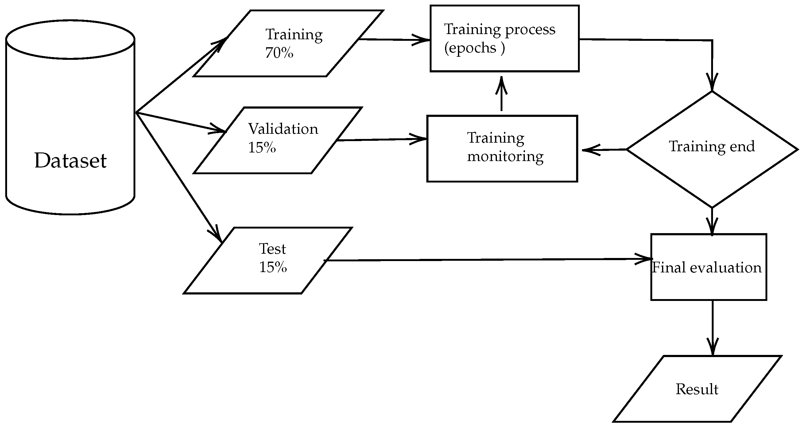
The training, validation, and test process is described in Figure 3. It was implemented using the “nftool” App in MATLAB^® R2024a (The MathWorks, Inc., Natick, MA, USA).

Figure 3. Training, validation, and test process.

The data division is done for three datasets, training, validation, and testing, with the aim of ensuring an accurate and generalizable model using a random order to avoid bias. This division is carried out as follows: 70% for training, which adjusts the model weights using the Levenberg–Marquardt algorithm, optimizing the error function; 15% for validation, which monitors the model’s performance during training, helping to prevent overfitting by stopping the process when the error in this set begins to increase; and 15% for testing, which evaluates the model’s generalization ability, providing a final measure of performance.

Performance is obtained by calculating the average quadratic difference between outputs and target values (MSE); the closer to zero, the better the performance [56].

2.3. Tabu Search

The heuristic technique used to solve combinatorial optimization problems is considered one of the most efficient techniques, finding quality solutions in the shortest amount of time [57]. The Tabu Search Algorithm 1 based on creating a T set of Tabu movements and an evaluation function denoted by OPTIMUM, proposed by [58], is described below.

Algorithm 1 Simple Tabu Search

Select an initial x ∈ X and let x* := x. Set the iteration counter k = 0 and begin with T empty. If S(X) − T is empty, go to Step 4. Otherwise, set k := k + 1 and select $s_k$∈ S(X) − T such that $s_k$ = OPTIMUM(s(x):s ∈ S(X) − T). Let x := $s_k$(X). If C(X) < c(x*), where x* denotes the best solution currently found, let x* := x. If a chosen number of iterations has elapsed either in total or since x* was last improved or if S(x) = 0 upon reaching this step directly from Step 2, stop. Otherwise, update T and return to Step 2.

The Tabu Search algorithm has mechanisms that allow movements to be found locally; it also uses a temporary memory, called Tabu list, where it stores the recent search and thus avoids getting past solutions. Although the Tabu Search mechanism prevents cycling and improves the exploration of the search space, it is a heuristic optimization method and therefore does not guarantee convergence to the global optimum.

2.4. Auto-Design

Two of the essential features to consider in the choice and design of the neural network described in two steps [50]:

1.

The network’s structural design determines the layer’s numbers and neurons in each layer and the transfer function.

2.

Selection of training methods and corresponding parameters. Network training or determination of free network parameters.

Sometimes, network training performance depends mainly on its structure/topology. Despite its importance, few methods are available for selecting the topology of a neural network, and most of these methods are based only on iterative procedures and evolutionary models [50,53,59,60].

2.5. Travel Time

The prediction of travel time in urban areas has been of great interest, and new research began to develop a few decades ago compared to motorway travel time [38,61]; this is due to the existence of more significant variables that affect travel time. Travel time is defined as follows [62].

Definition 1. 

Individual travel time on an r route at departure time t is the time it takes for a traveler (driver, pedestrian, passenger) to cross that particular route.

2.6. Methods

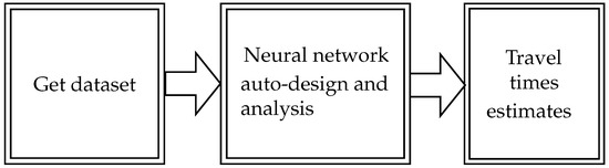
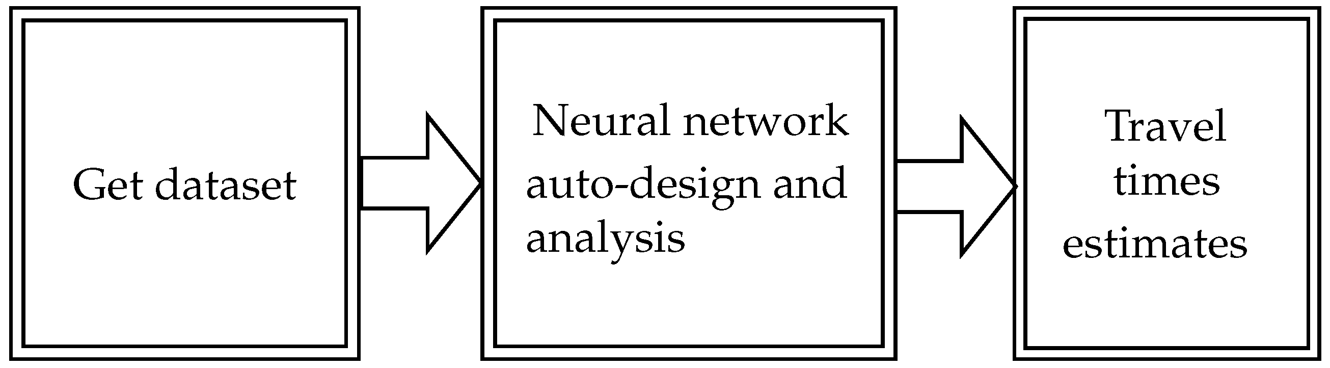
The proposed model is structured in three key phases for predicting travel time, as shown in the diagram (Figure 4). The first phase is obtaining the dataset, which is based on a detailed study of the variables that affect travel time, such as traffic, weather conditions, and road infrastructure.

Figure 4. Methodology for obtaining travel times.

The second phase involves the automatic selection of the artificial neural network (ANN) topology. In this phase, a proposed algorithm is responsible for automatically designing the optimal network architecture, adjusting the number of layers, neurons, and activation functions based on initial parameters. This process is performed periodically to keep the model up to date.

The third phase consists of estimating the coefficients or travel times for each edge of the street network. Unlike the first two phases, which are performed periodically, this phase is executed just before a route is plotted, providing accurate and up-to-date travel times for optimal decision-making.

2.6.1. Proposed Auto-Design of ANN Topology (A-DANNT) Algorithm

In the network’s topology, the inputs are considered variables; these are defined as dynamics concerning time, which constantly update and modify the dataset. This paper proposes an algorithm that designs the topology automatically, obtaining architectures that adapt to the input data. The determination of the optimal topology is defined as a constrained optimization problem over discrete hyperparameters:

$$(i^{*},j^{*})=arg\underset{i,j}{max}{R}_{i,j}\mathrm{s}.\mathrm{t}.j\le Nnm+6\Delta ,i\le Nlm+1$$

(8)

where i represents the number of layers and j represents the number of neurons. The proposed algorithm for the auto-design and choice of the best topology for regression problems is shown in Figure 5. The parameters used in the algorithm are defined as follows:

• $n.min$ is the minimum number of neurons with which the algorithm starts.
• $\Delta$ is the neuron increment factor, which influences the convergence speed.
• $i,j$ are the current layer and number of neurons being evaluated.
• $r_{i,j}$ is the correlation coefficient (R-value) for each architecture $i,j$.
• m is the best R-value found during the search.
• $Nnm,Nlm$ are the neuron and layer counts of the best architecture discovered ($j^{*}$ and $i^{*}$).
• $N.neurons,N.lay$ are the variables representing the current topology state.

Figure 5. The proposed auto-design algorithm flow diagram.

Figure 5. The proposed auto-design algorithm flow diagram.

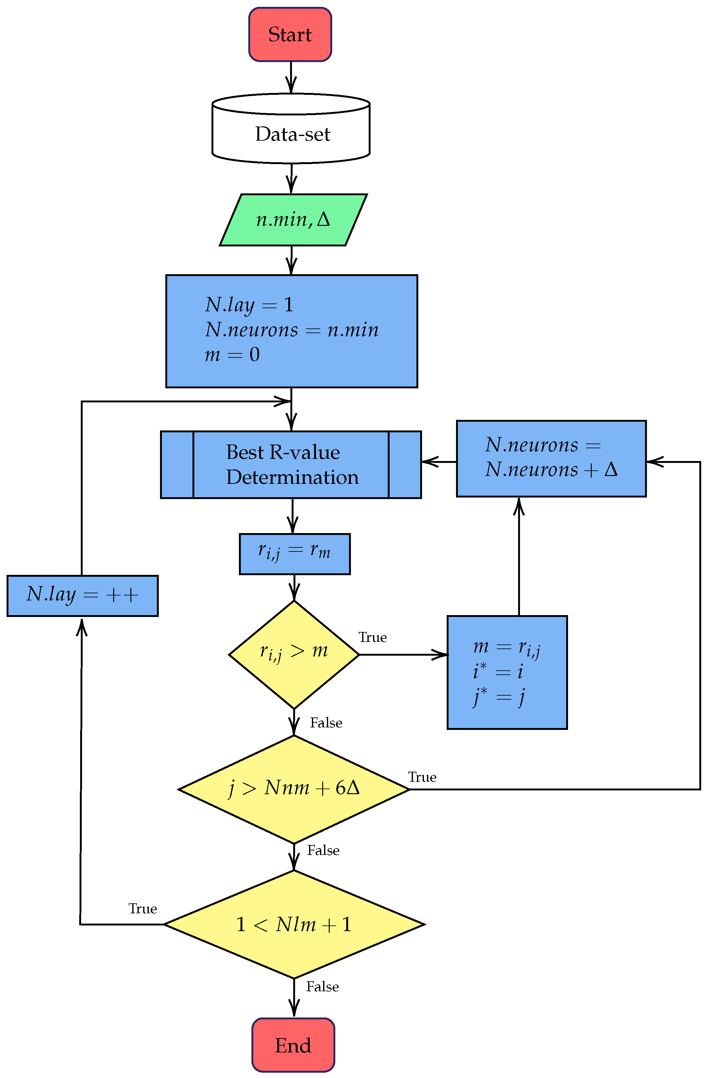
The algorithm starts by entering the dataset. The next step requests a neuron number to initialize ($n.min$) and an increment factor $\Delta$. Initially, a minimum of 10 neurons and an increment factor of 10 are proposed. In the next step, $N.lay$ is initialized with one, $N.neurons$ with $n.min$, and m (the best R-value) with zero.

A process is then carried out to determine the best correlation coefficient using the BR-vD algorithm. The architecture is iteratively optimized by updating $r_{i,j}$ with the value $r_m$ obtained from the training process. If $r_{i,j}>m$, the values of m, $Nlm$, and $Nnm$ are updated, and $N.neurons$ is incremented by $\Delta$. The search for neurons within a layer follows the termination condition $j>Nnm+6\Delta$, ensuring that the process ends after six continuous iterations without improvement in the R-value.

The process repeats iteratively until the layers’ number ($N.lay$) reaches the limit condition ($N.lay<Nlm+1$). The algorithm increases one layer when the R-value rate does not improve in six continuous iterations and stops the design if more than two continuous layer increments do not improve.

2.6.2. Proposed Best R-Value Determination Algorithm (BR-vD)

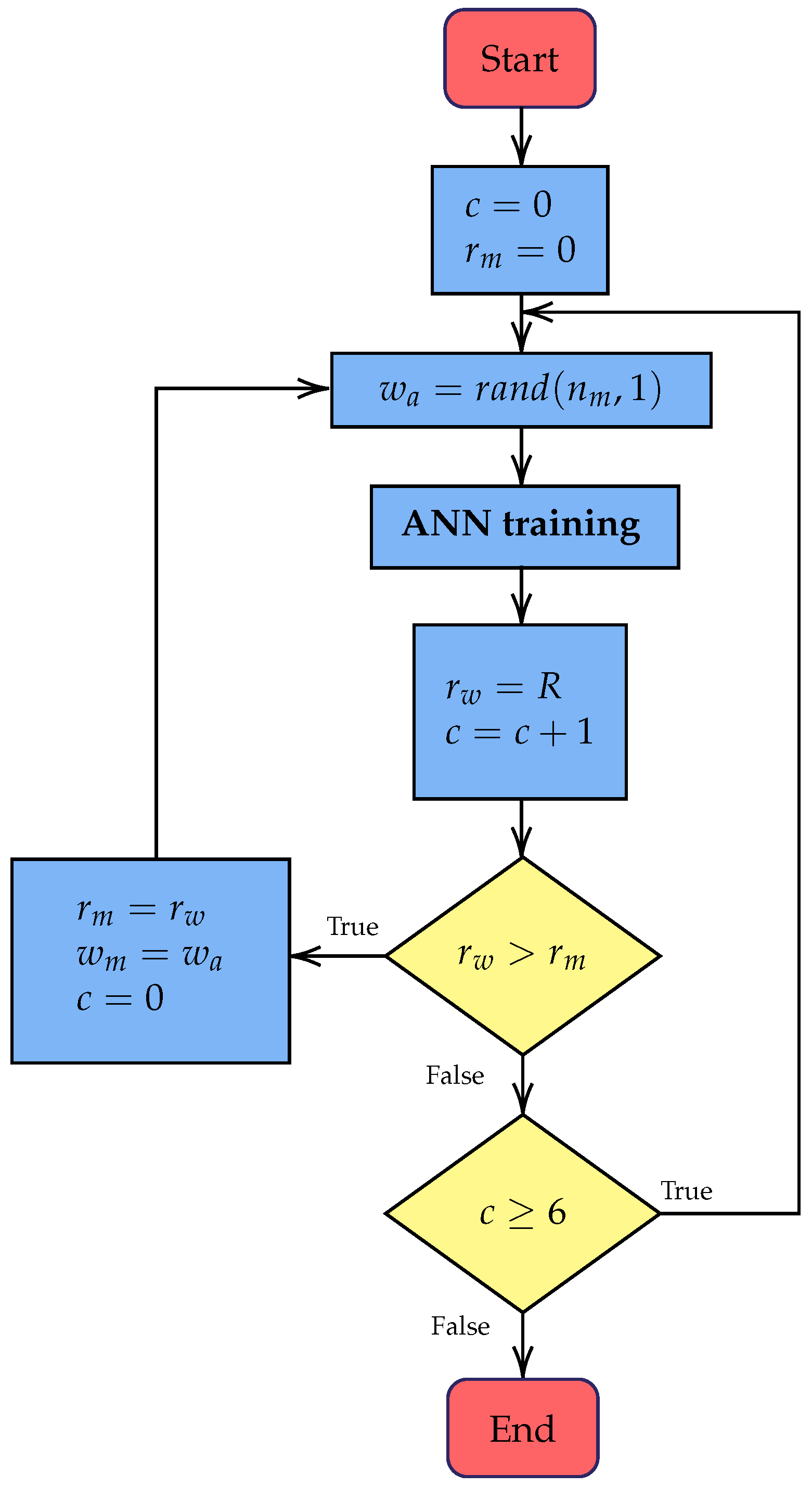
The objective is to obtain the initial synaptic weights w for each analyzed topology by searching for a configuration that yields the highest R-value. Figure 6 illustrates the flowchart of the Best R-Value Determination (BR-vD) algorithm based on Tabu Search. Based on the Tabu Search heuristic, the selection of the best movement in each iteration is formally represented as

$$x^{(k+1)}=arg\underset{s\in S\left(x^{\left(k\right)}\right)\setminus T}{min}C\left(s\right)$$

(9)

where $S\left(x^{\left(k\right)}\right)$ is the neighborhood of solutions, T is the Tabu list, and $C\left(s\right)$ is the cost function, in this case, the Mean Square Error (MSE). The algorithm assigns 0 to the counter c and initializes $r_m=0$. A vector of random synaptic weights $w_a$ is generated. Levenberg–Marquardt backpropagation is applied to train the ANN, using a dataset division of 70% for training, 15% for validation, and 15% for testing. If the correlation $r_w$ from the test set is greater than $r_m$, the best weights $w_m$ are updated and c is reset to zero. The algorithm follows the termination condition $c\ge 6$, concluding the search for a specific topology if no improvement is found in six consecutive iterations. The variables involved are

• $r_m$ is the best correlation coefficient (global variable).
• c is the stagnation counter for the termination condition.
• $r_w$ is the correlation coefficient of the current iteration (local variable).
• $w_a$ is the vector of random weights generated in each move.
• $w_m$ is the vector of weights corresponding to the best solution found.

Figure 6. BR-vD algorithm flowchart.

Figure 6. BR-vD algorithm flowchart.

2.7. Computational Complexity Analysis

To evaluate the scalability of the proposed A-DANNT and BR-vD algorithms, a complexity analysis is performed. The computational cost is primarily determined by the iterative process of training neural networks with varying architectures.

For a network configuration with i layers and j neurons per layer, the approximate number of trainable parameters P (synaptic weights and biases) is given by

$$P\approx O(i·j^2)$$

(10)

This quadratic relationship arises because each layer in the multilayer perceptron is fully connected to the subsequent layer. The training process utilizes the Levenberg–Marquardt algorithm, which involves solving a linear system based on the Jacobian matrix. This results in an approximate computational cost per training iteration of

$$O\left(P^2\right)$$

(11)

Consequently, the overall complexity for evaluating a single candidate architecture can be estimated as

$$O(i^2·j^4)$$

(12)

Since the A-DANNT algorithm explores multiple configurations, the total execution time scales with the number of explored architectures. However, the implementation of a stopping criterion ($c\ge 6$) based on consecutive non-improving iterations effectively prunes the search space, preventing an exhaustive search and ensuring the practical scalability of the system for urban-scale travel time prediction.

2.8. Algorithm Analysis and Convergence

Since the proposed search strategy is based on the Tabu Search metaheuristic, it explores the discrete hyperparameter space efficiently. As with heuristic optimization methods, mathematical convergence to the global optimum cannot be guaranteed. Instead, the algorithm seeks a stable topology by monitoring the improvement in the correlation coefficient (R).

The stopping criterion based on six consecutive non-improving iterations ($c\ge 6$) serves as a practical convergence indicator. The choice of $c=6$ represents an empirical compromise between two factors:

• Exploration: allowing sufficient iterations to escape local optima and evaluate neighborhood variations.
• Efficiency: avoiding the evaluation of architectures that are structurally similar and provide comparable performance.

Considering that the computational cost grows with the number of layers and neurons, the stopping rule effectively limits redundant evaluations in the architecture search. Therefore, it acts as a regularization mechanism that prunes the search space while maintaining consistent predictive performance.

2.9. Hyperparameter Selection and Tuning Strategy

To improve reproducibility, the hyperparameters are divided into fixed training parameters and adaptive architectural parameters. The A-DANNT search process automatically determines the number of hidden layers and the number of neurons, while the optimizer configuration remains fixed to allow consistent comparison among candidate topologies.

Training is performed using the Levenberg–Marquardt (LM) algorithm. The damping factor $\mu$ and its update coefficients were maintained at commonly used stable values ($\mu =0.001$, increase factor of 10, decrease factor of $0.1$), since the objective of this work is to analyze topology adaptation rather than optimizer tuning.

The adaptive parameters include the neuron increment factor $\Delta$ and the stopping criterion $c=6$. These values were empirically calibrated to balance the exploration of candidate architectures and computational cost. Smaller values tend to stop the search prematurely, while larger values lead to repeated evaluation of similar topologies.

This separation between fixed optimizer settings and adaptive topology search allows performance differences to be primarily associated with the architecture selection process rather than manual parameter adjustment.

2.10. Real-Time Implementation Feasibility

The practical application of the A-DANNT framework involves two distinct phases: offline auto-design and online prediction. The training phase, which includes the Tabu-based search for the optimal topology, is performed offline. For the 10,000-observation dataset, the total training process required approximately 35 min on a standard desktop computer (Intel Core i7, 16 GB RAM). This stage is only required during initialization or when the model is updated with new data.

In contrast, the prediction phase operates in real time. Once the optimal architecture is obtained, generating a travel time prediction for a new input vector only requires a forward propagation through the neural network. The measured inference time was below 1 ms per sample. Considering that typical traffic monitoring systems operate with sampling intervals of seconds or minutes, the computational cost of prediction is negligible relative to the acquisition period, making the approach compatible with real-time Intelligent Transportation System (ITS) deployments.

3. Experiments and Computational Results

3.1. Case Study 1

3.1.1. Parameters

This study carries out operations of fast food delivery vehicles in the city of Tuxtla Gutiérrez, Chiapas, Mexico; the study detects 52 factors. This analysis identifies those whose behavior is uncertain, more often, with a significant relationship affecting the distribution process.

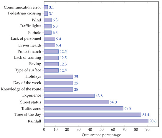
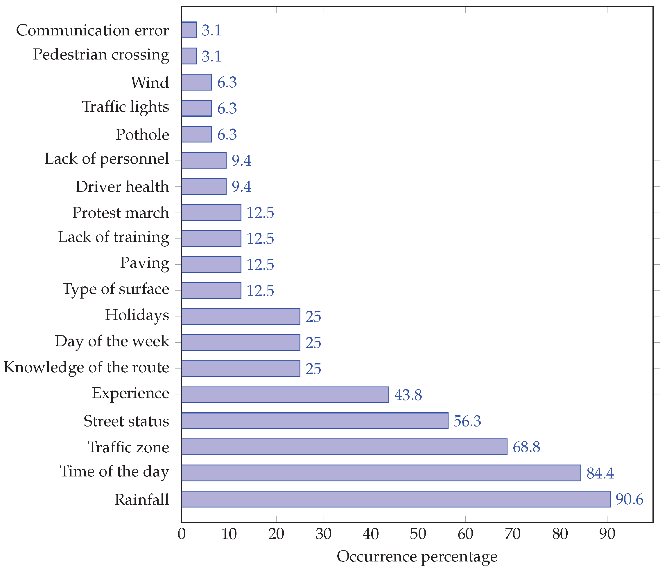
This study considers different aspects of the distributors such as age, job seniority, driving seniority, hours with the highest number of orders, delivery strategies, orders on the same route, order strategies on the same route, and reasons for late deliveries. The operators chose the factors that significantly affect timely delivery and late deliveries. Figure 7 presents a summary of the study, considering only the factors that affect delivery in order from least to most significant affectation; with the results obtained, the variables are classified according to the degree of affectation and the frequency at which they show up.

Figure 7. Factors considered in the product delivery.

Derived from the previous study and taking as reference the value of the street distance, this work proposes five parameters, which modify each side of the network’s travel time, as described below [63]:

• Time of day (Td): the time the order is placed, confirmed by the company’s service schedule, from 9:00 to 23:00 (GMT-6) time of the city in Mexico.
• Street distance (Sd): considered the street’s distance from one node or corner to another (m).
• Street status (Ss): defines the amount and size of obstacles that vary the vehicle’s speed (speed bump, potholes, bad sewer, street deformations, repairs, and maintenance). The variable $Ss$ is obtained from a study of delivery operators providing the type and size of obstacles. This study is carried out in the city of Tuxtla Gutiérrez, Chiapas, Mexico, where speed bumps are commonly found; potholes, each with levels of small, medium, and large; in addition to sewage in poor conditions, street deformations caused by subsidence, repairs, or maintenance, each with partial, half, and total levels (see Table 1).
• Traffic zone (Tz): is considered the density of vehicle circulation in the streets due to the proximity of school areas, shopping centers, or areas that make traffic difficult. The zones with the highest traffic were identified at a particular time with the highest influx of vehicles in Tuxtla Gutiérrez, Chiapas, Mexico (see Table 2).
• Rainfall (Rl): is the amount of water precipitation that causes a decrease in visibility and speed (mL/m²). The pluvial precipitation data provided by the General Coordination of the National Meteorological Service (CGSMN by its acronym in Spanish Coordinación General del Servicio Meteorológico Nacional) of the National Water Commission (CONAGUA by its acronym in Spanish Comisión Nacional del Agua) are used, registered in the observatory and the automatic meteorological station (ESIME by its acronym in Spanish Estación Sinóptica Meteorológica); the data are collected from 1980 to 2010 in the city of Tuxtla Gutiérrez, Chiapas, Mexico.

Table 1. Street status.

Street Status	Identifier	Street Status	Identifier	Street Status	Identifier
no obstacles	0	one medium-sized pothole	10	two large speed bumps	20
one small pothole	1	three small potholes	11	two big potholes	21
one small speed bump	2	three small speed bumps	12	one big pothole	22
two small potholes	3	one large speed bump	13	three or more large speed bumps	23
two small speed bumps	4	two medium-sized speed bumps	14	big street deformations	24
sewer tap is partially in poor condition	5	two medium-sized potholes	15	sewer tap is totally in poor condition	25
three small pothole	6	partial street repairing	16	three or more big potholes	26
one medium-sized pothole	7	sewer tap is poor condition in mid	17	totally street repairing	27
partial street deformations	8	three medium-sized speed bump	18
medium-sized street deformations	9	mid street repairing	19

Table 2. Traffic zone identifier.

Traffic Zone	Identifier
no zone	0
banks	1
supermarket	2
shopping centers	3
school areas	4

3.1.2. Dataset

The dataset used in this research was constructed from 10,000 observations collected from real delivery routes monitored under normal operating conditions in Tuxtla Gutiérrez, Mexico. The proposed work consists of two datasets, input and output (target); the input contains the five parameters described above, and the output is the calculated travel time for each street segment.

The data acquisition process involved a combination of digital recording and manual annotation. Each trip was monitored using mobile tracking devices to obtain precise travel time and distance ($S_d$) through GPS measurements. Environmental and traffic variables were annotated in situ at the moment of the trip. Specifically, the variable Street Status ($S_s$) was determined using a standardized visual inspection protocol performed by the operators, who identified the type, size, and frequency of obstacles such as speed bumps, potholes, and road repairs.

These observations were encoded into a discrete ordinal scale ranging from 0 to 27, as detailed in Table 3, where 0 represents a route with no obstacles, and higher values indicate increasing complexity in road conditions. Before the dataset enters the training process, it undergoes organizational treatment and data augmentation to ensure model robustness.

Table 3. Dataset example, case 1.

Street Distance (m)	Street Status	Traffic Zone	Time of the Day	Rainfall (mL/m2)	Travel Time (s)
102	0	0	11	3	4.7414
140	0	0	12	11	8.0410
150	0	0	21	60	11.3966
280	0	0	18	21	13.0509
206	3	0	17	7	21.4261
276	0	4	7	46	29.3480
151	2	1	22	1	32.9279
125	11	1	9	52	69.4985

For the analysis of the problem, street network values are used, taking Table 4 as a reference. In the first column, the length ($S_d$) of each street varies from 50 to 500 m. The traffic zone ($T_z$) values are categorized from 0 to 4 based on the municipal traffic classification map. The time of day ($T_d$) represents the hour of measurement, and rainfall ($R_l$) denotes the precipitation level at the time of reading. The final columns of the dataset compare the actual travel time values with the network’s predictions to calculate the differences.

Table 4. Output values (target) vs. predicted values.

Street Distance (m)	Street Status	Traffic Zone	Time of the Day	Rainfall (mL/m2)	Travel Time (s)	Travel Time Prediction	Difference
102	0	0	11	3	4.7414	4.9356	0.1942
140	0	0	12	11	8.0410	7.0643	0.9767
150	0	0	21	60	11.3966	8.7412	2.6554
280	0	0	18	21	13.0509	12.5539	0.497
206	3	0	17	7	21.4261	26.2508	4.8247
276	0	4	7	46	29.3480	32.6712	3.3232
151	2	1	22	1	32.9279	31.8730	1.0549
125	11	1	9	52	69.4985	68.7611	0.7374

The observations were collected over a period of approximately 6 months under regular operational schedules. Each record corresponds to a completed street traversal event; therefore, the dataset follows an event-based sampling scheme rather than a fixed temporal sampling frequency. Consequently, the temporal spacing between consecutive observations varies according to real traffic operation conditions.

The candidate variables were initially identified from operational context. Subsequently, their relevance was verified through occurrence distribution analysis (Figure 7) and model predictive behavior. Variables with high presence in the operational records ($R_l$, $T_d$, $T_z$, $S_s$) correspond to the dominant variability affecting travel time, while low-frequency factors behave as sporadic disturbances and do not contribute to predictive improvement.

Thus, the selected inputs are supported by both domain knowledge and data behavior, ensuring that the model structure is driven by the principal dynamics of the system rather than subjective selection.

3.1.3. Input Variable Dimensionality Considerations

The street status variable is defined by 28 discrete categories representing specific road and traffic conditions (e.g., free flow, potholes, or obstacles). These categories are mutually exclusive, meaning that only one condition is active at each observation. Therefore, although the encoding expands the representation across several components, the effective information dimensionality remains low because the variable behaves as a single categorical descriptor in the traffic context.

Moreover, the A-DANNT architecture search mechanism automatically adjusts the hidden layer configuration based on the statistical contribution of the inputs. This adaptive process matches the model capacity to the informative content of the categorical data, mitigating overfitting and reducing the impact of redundant representation. Consequently, the framework introduces an implicit regularization effect that optimizes the mapping between heterogeneous input variables and travel time prediction.

3.1.4. Network Description, Case 1

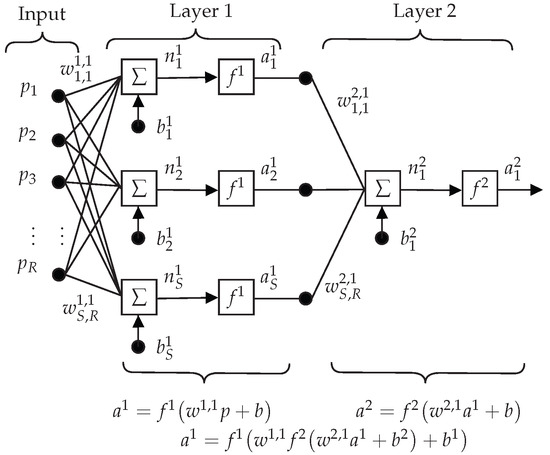
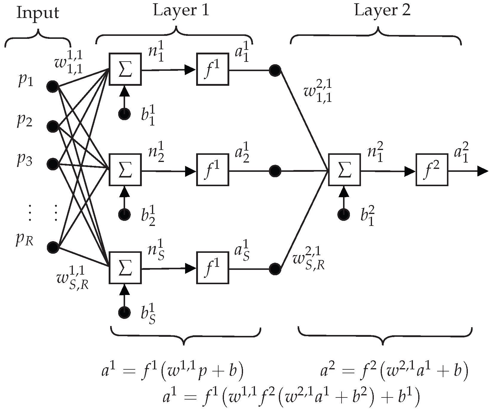
Figure 8 shows the network proposed by the A-DANNT algorithm; each layer contains an array of weights w, a bias vector b, and an output vector a. $P_R$ equals the number of inputs, where

Figure 8. Neural network model for travel time determination.

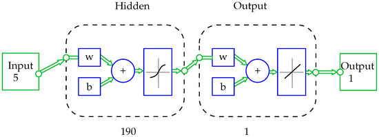
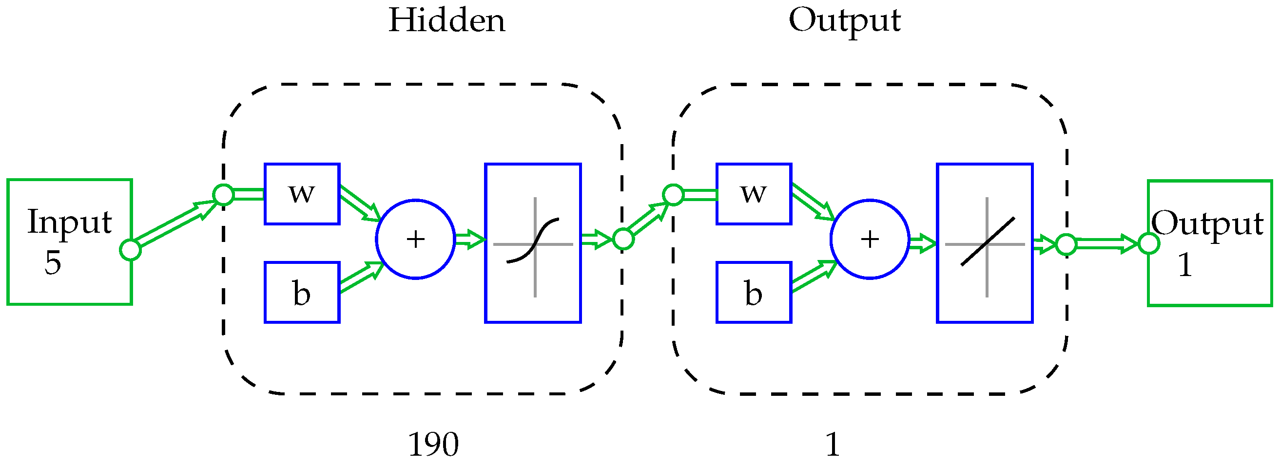
R equals five; S is the number of neurons for each layer (190 for the hidden layer and one for the output layer); the hidden layer f equals the activation functions, Sigmoidal for the hidden layer, and linear function for the output layer. ©MATLAB draws the two-layer network using the abbreviated notation in Figure 9.

Figure 9. Proposed neural network by A-DANNT.

3.1.5. Results Analysis 1

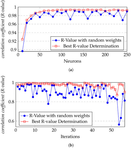
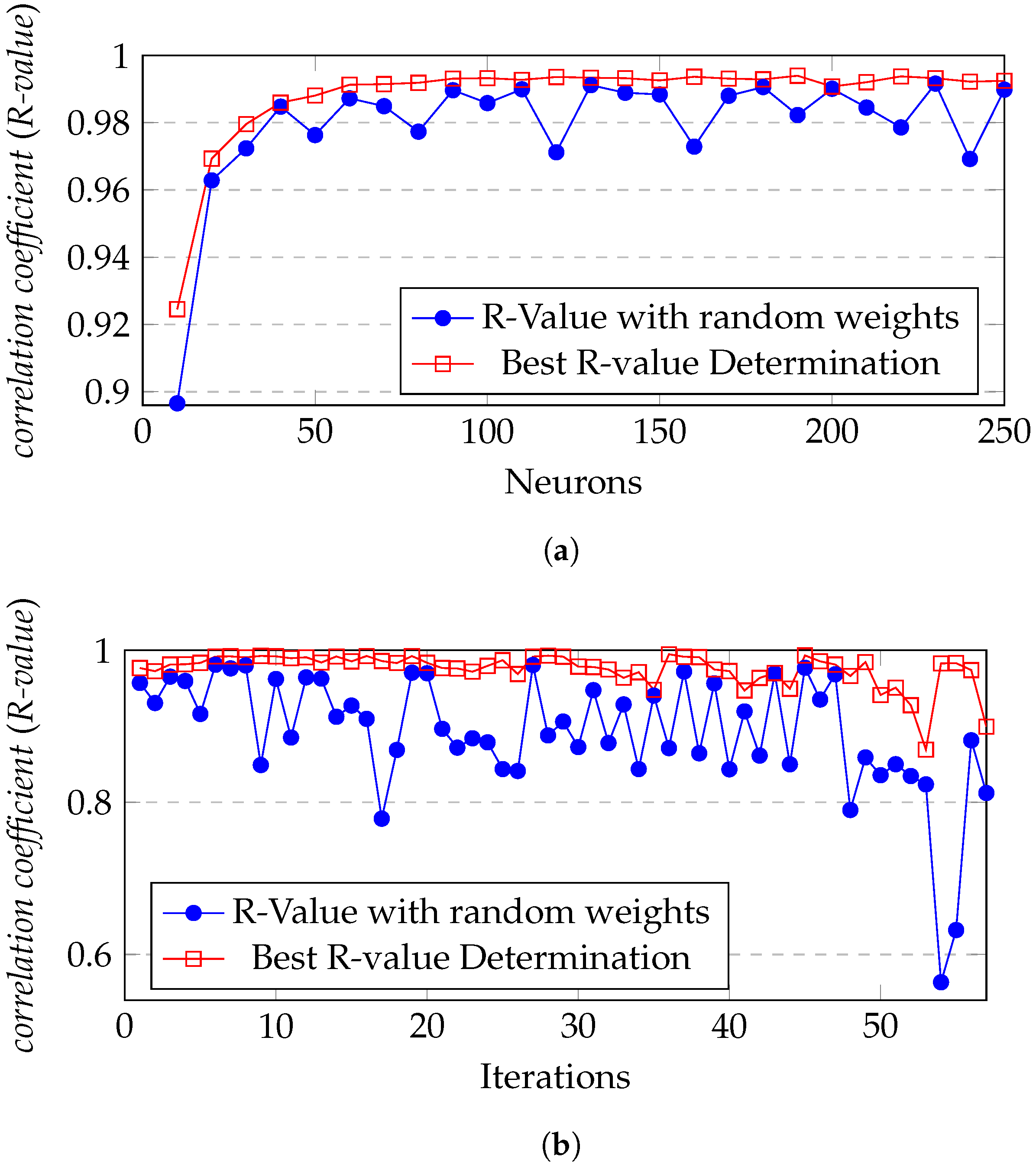
The algorithm chooses the best R-value correlation coefficient of different topologies; Figure 10 graphically shows the comparison and choice of the correlation coefficient of the different topologies, using a set of random weights (blue circles) and a dataset provided by the BR-vD algorithm (red squares). Figure 10a shows an R-value set for one layer, with neurons in the range of 10, 20, 30, …, 250. Figure 10b shows a set of R-values for two layers with combinations in the range of 10–10, 10–20, …, 70–20, 70–30. Table 5 shows a part of the process of choosing and storing weights w with one layer.

Figure 10. Comparison of R-values for different topologies. (a) One layer; (b) two layers.

Table 5. Values analysis.

Iteration Numbers	${\mathit{w}}_{\mathit{a}}$	${\mathit{r}}_{\mathit{m}}$	${\mathit{R}}_{\mathit{w}}$ = R-Value	List R	List ${\mathit{w}}_{\mathit{m}}$
1	$w_1$	0	0.98338	[0.98338]	[$w_1$]
2	$w_2$	0.98338	0.98869	[0.98338, 0.98869]	[$w_1$, $w_2$]
3	$w_3$	0.98869	0.99344	[0.98338, 0.98869, 0.99394]	[$w_1$, $w_2$, $w_3$]
4	$w_4$	0.99344	0.98873	[0.98338, 0.98869, 0.99394]	[$w_1$, $w_2$, $w_3$]
5	$w_5$	0.99344	0.99238	[0.98338, 0.98869, 0.99394]	[$w_1$, $w_2$, $w_3$]
6	$w_6$	0.99344	0.99366	[0.98338, 0.98869, 0.99394, 0.99394]	[$w_1$, $w_2$, $w_3$, $w_6$]
7	$w_7$	0.99366	0.99139	[0.98338, 0.98869, 0.99394, 0.99394]	[$w_1$, $w_2$, $w_3$, $w_6$]
8	$w_8$	0.99366	0.99204	[0.98338, 0.98869, 0.99394, 0.99394]	[$w_1$, $w_2$, $w_3$, $w_6$]
9	$w_9$	0.99366	0.99236	[0.98338, 0.98869, 0.99394, 0.99394]	[$w_1$, $w_2$, $w_3$, $w_6$]

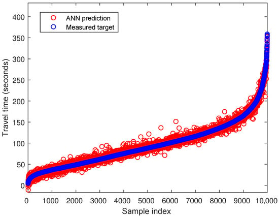
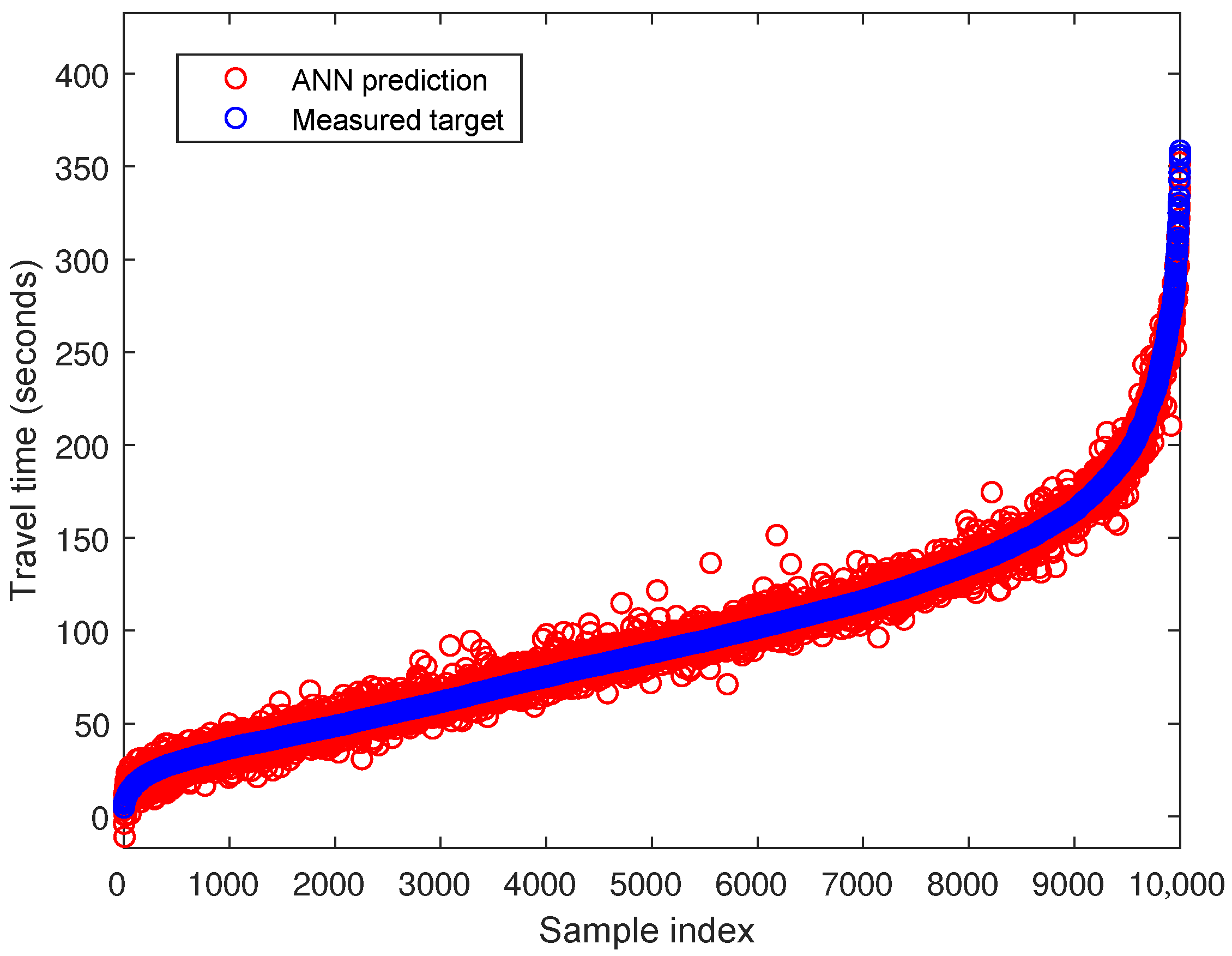
During the training process, the ANN gets an error for each topology; if the error increases as it reaches the maximum of times, it will cause an over-adjustment; the configuration stops the process after six consecutive increases and takes the lowest error. The values estimated by the neural network are compared with the desired values, predicting any value from the output dataset. Figure 11 shows the comparison of the desired values with the values estimated by the trained network, estimated travel time (y), and dataset (x), where the MSE is 22.51 s. The MSE is the mean of the squared difference between the network output and the desired value; the smaller the value, the better the prediction.

Figure 11. Predicted vs. measured travel times over the complete dataset.

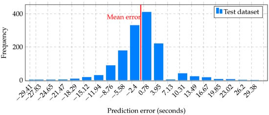
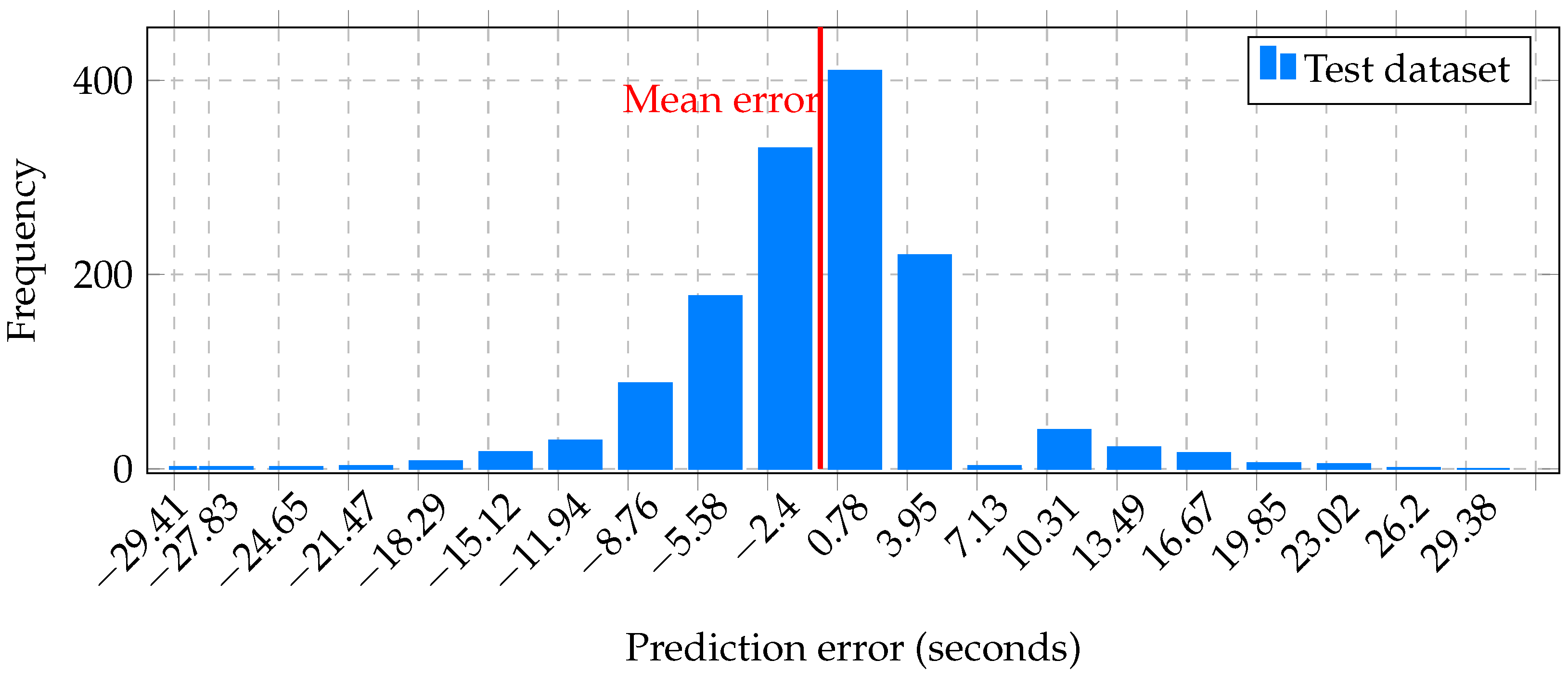
Figure 12 shows the frequency or trend of the error graphically (the desired output minus the actual output) with 20 bars, where the test dataset locates and the red line represents the mean error.

Figure 12. Distribution of prediction error on the test dataset.

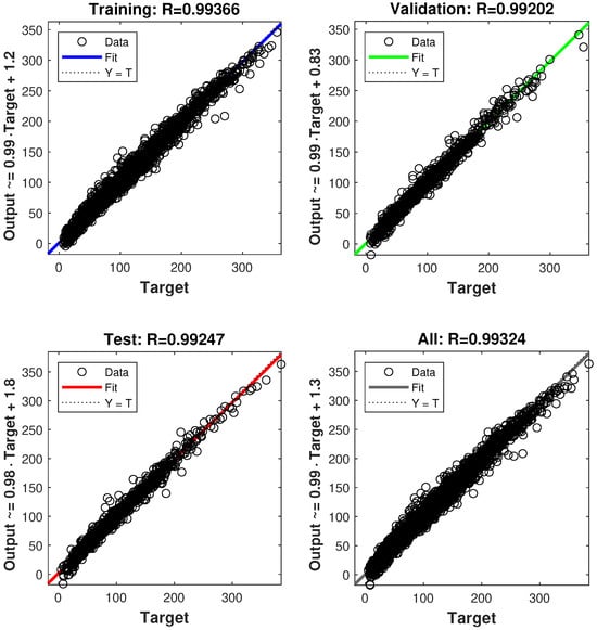
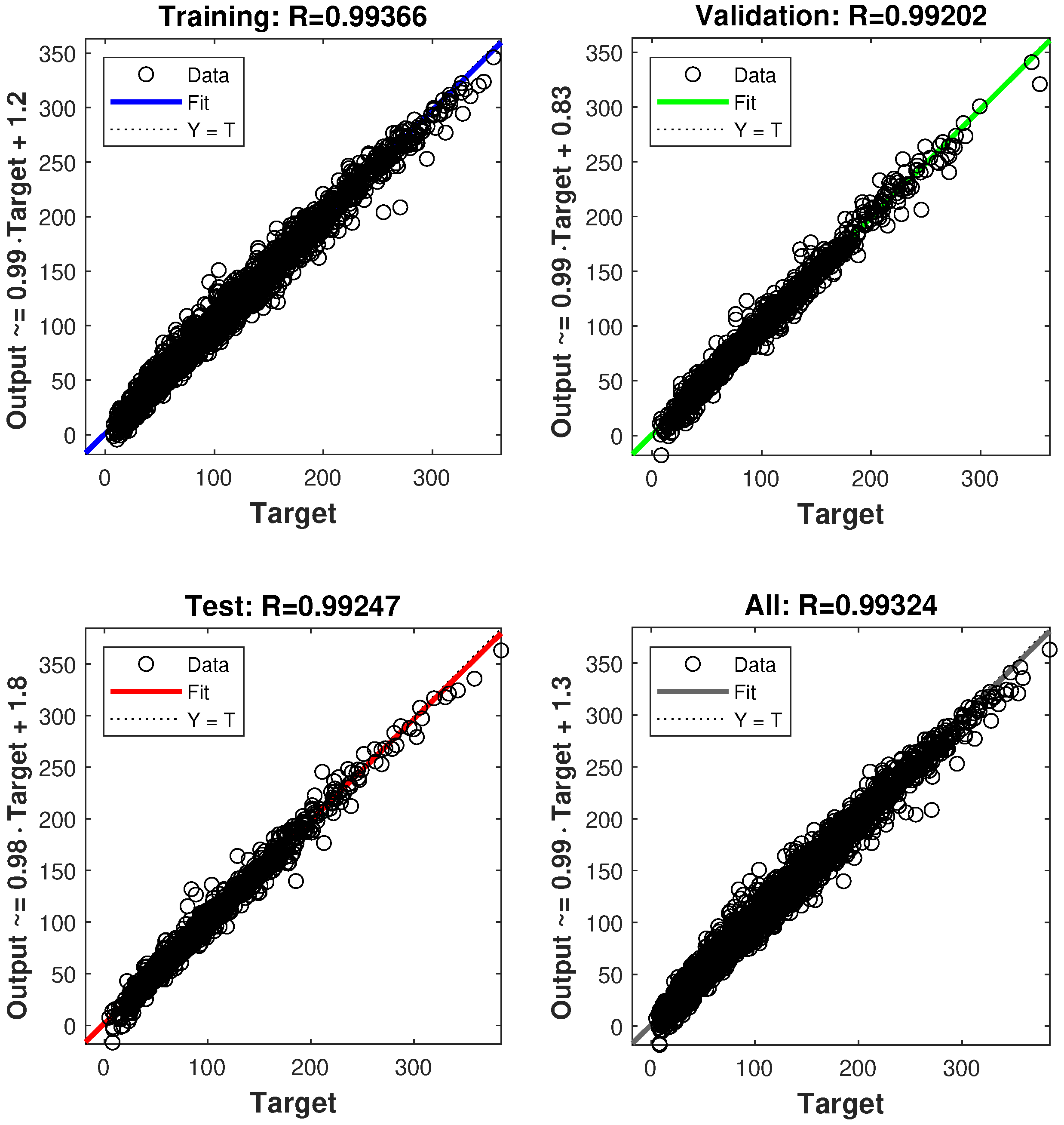
Figure 13 shows the linear regression analysis for the training, validation, test, and full datasets in case 1. The dotted line represents the ideal relationship $outputs=targets$, while the continuous line corresponds to the best-fit regression between outputs and targets. The obtained correlation coefficients are $R=0.99366$ (training), $R=0.99202$ (validation), $R=0.99247$ (test), and $R=0.99324$ (all data). The similar values across the three independent subsets indicate consistent predictive behavior and confirm that the model performance is not dependent on a particular data partition.

Figure 13. Linear regression analysis for case 1 showing training, validation, test, and full dataset performance.

To contextualize the proposed method within automated model design approaches, we compare A-DANNT with regression models optimized through Bayesian optimization (Table 6). This strategy represents a common AutoML paradigm where model parameters are tuned while keeping the architecture fixed.

Table 6. Performance comparison with regression models optimized using Bayesian optimization.

Method	SVM	Gaussian Process	Tree	Ensemble LSBoost	Proposed A-DANNT
RMSE (s)	9.6710	9.1937	9.1751	9.0612	6.4354

Table 6 shows that the A-DANNT model achieves a significantly lower Root Mean Square Error (RMSE) compared to other optimized machine learning approaches.

It is important to clarify the exclusion of certain deep learning architectures like Long Short-Term Memory (LSTM), Gated Recurrent Units (GRUs), or Transformers. These models are specifically designed to exploit temporal dependencies in sequential data. However, the dataset utilized in this study consists of independent trip observations where each sample is described by a set of static contextual variables (distance, road status, etc.) without a sequential relationship between consecutive records. Consequently, sequence-based models do not offer a structural advantage for this prediction task, and the A-DANNT algorithm remains the most appropriate framework for this tabular regression problem.

3.2. Case Study 2

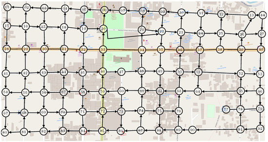
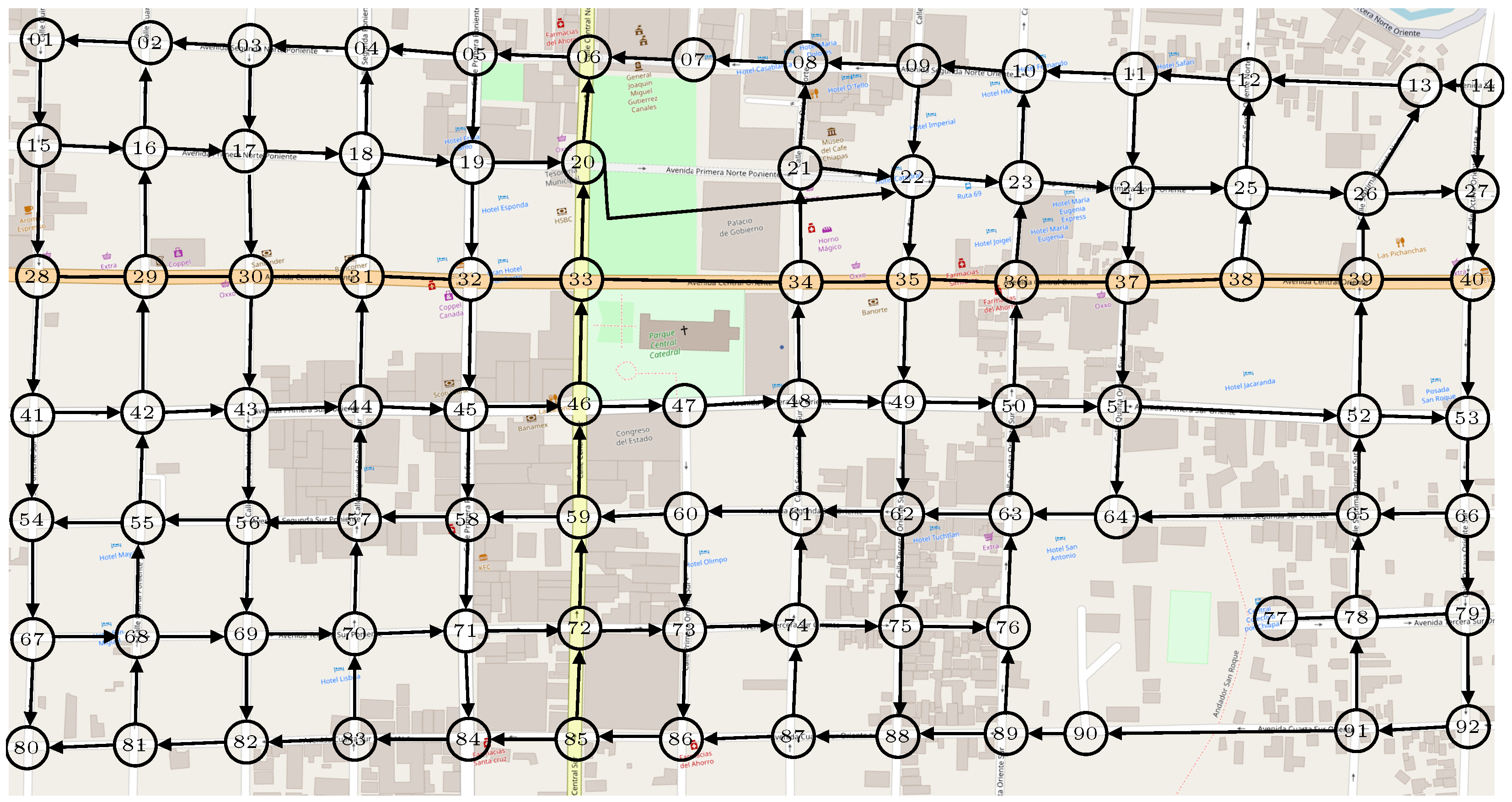
The auto-design algorithm obtains the ideal topology for any regression problem; the following case study uses the data presented by [34]. The authors calculate the travel times of a routing problem for a delivery company in Tuxtla Gutiérrez, Chiapas, Mexico. Figure 14 shows the delimited area of the city and the nodes that represent the corners, where the objective is to calculate the travel times for all the edges of the street network and then obtain the shortest route from source node 15 to destination node 43. The authors, in their model, propose fuzzy conditions, a variable, Time taken to cross street corners (see Table 7), the Traffic Coefficient, and the time of day; these variables adjust the travel time.

Figure 14. Road network of the application zone with numbered nodes and traffic flow directions. The highlighted path indicates the analyzed route.

Table 7. Time taken to cross street corners [34].

Type of Street Corner	Time in Seconds
Traffic light (Tl)	50
Traffic light turn right (Tlr)	53
Traffic light turn left (Tll)	57
No preference (Np)	8
Preference (P)	3
Preference turn right (Pr)	6
Preference turn left (Pl)	7
One for one (O)	4
One for one turn right (Or)	6
One for one turn left (Ol)	6

For this case study, the street distance, time of day, Traffic Coefficient, and the Time taken to cross street corners are taken as the input variables to the neural network, using the category configuration (one hot). In this case, only the variables street distance, time of day, Traffic Coefficient, Ox, Or, Ol, Px, Pr, Pl, and Tlx Tlr are used as inputs; these variables make up the input dataset, and the travel time represents the output. Table 8 shows part of the dataset.

Table 8. Dataset example, case 2.

Street Distance	Time of Day	Traffic Density	Ox	Or	Ol	Px	Pr	Pl	Tlx	Tlr	Total Time
23	23:08:05	1	0	0	0	1	0	0	0	0	5.40833333
84	21:47:33	2	0	0	0	1	0	0	0	0	8.41875
80	21:47:33	2	1	0	0	0	0	0	0	0	12.4291667
86	21:47:33	2	0	0	0	0	0	0	1	0	55.41875
75	13:49:21	2.1	0	0	0	1	0	0	0	0	61.9303375
84	08:01:19	2.2	0	0	1	0	0	0	0	0	74.1161388
102	13:49:21	1.1	0	0	0	0	0	0	0	1	90.0607487
90	14:28:37	2.5	0	0	1	0	0	0	0	0	102.994709
212	13:49:21	2.1	1	0	0	0	0	0	0	0	163.953773

3.2.1. Network Description, Case 2

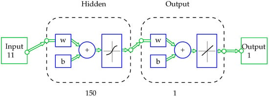
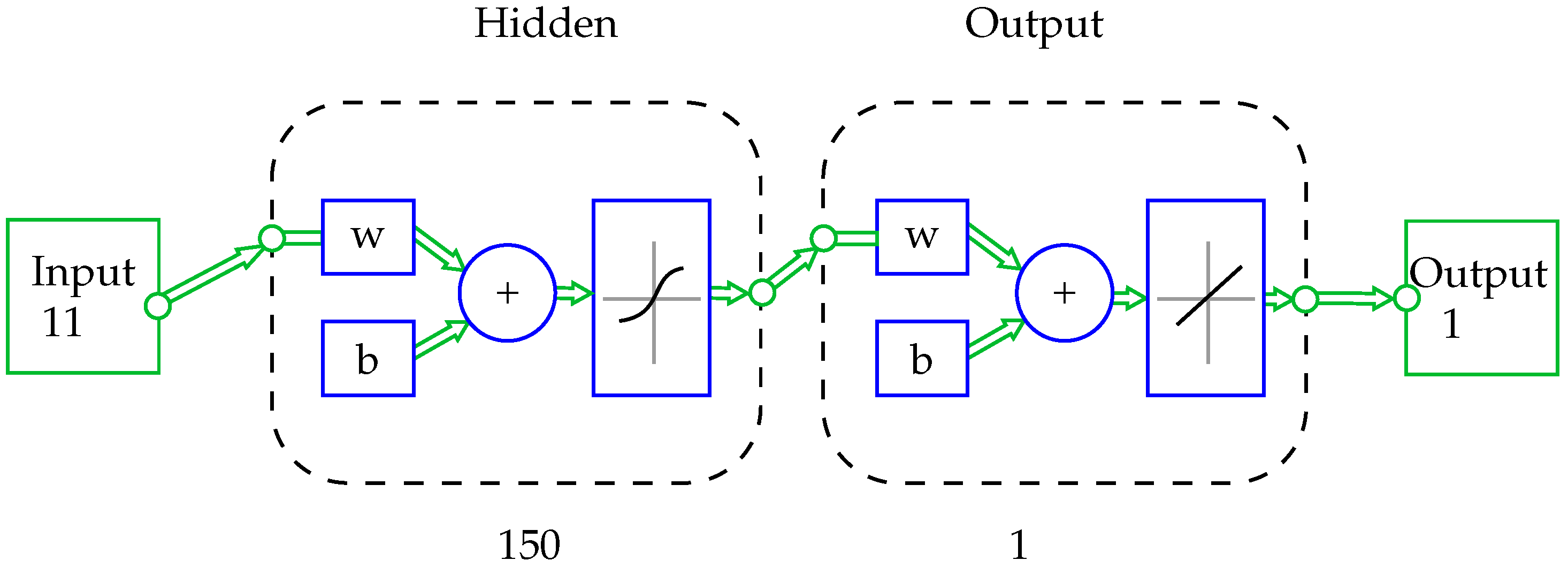
For case 2, the network proposed by the A-DANNT algorithm, each layer contains an array of weights w, a bias vector b, and an output vector a. $P_R$ equals the number of inputs, where $R=11$; S is the number of neurons for each layer (150 for the hidden layer and one for the output layer); the hidden layer f equals the activation functions, Sigmoidal for the hidden layer, and linear function for the output layer. ©MATLAB draws the two-layer network using the abbreviated notation in Figure 15.

Figure 15. Proposed neural network by A-DANNT, case 2.

3.2.2. Results Analysis 2

Table 9 presents the analysis of 21 routes presented by [34], as well as the schedule, the real-time, the one with calculated values using Fuzzy Linear Programming (FLP), the one predicted by the proposed neural network (A-DAANT), and the Absolute Percentage Error for FLP and A-DANNT compared to the real-time values. The analysis shows maximum and minimum values of 29.18% and 3.27%, respectively, a Mean Absolute Percentage Error of 9.6%, and the Variance of the Absolute Percentage Error of 46.57% for FLP. In comparison, the maximum and minimum values were 28.88% and 2.51%, the Mean Absolute Percentage Error was 7.95%, and the Variance of the Absolute Percentage Error was 36.24% for A-DANNT.

Table 9. FLP vs. A-DANNT Absolute Percentage Error.

Route	Schedule	Real Travel Time	Travel Time of the Fuzzy Model (FLP)	Absolute Percentage Error (FLP) %	Auto-Design Travel Time ANN (A-DANNT)	Absolute Percentage Error (A-DANNT) %
15-13	06:22:17	00:05:29	00:03:53	29.18	00:03:54	28.88
15-13	14:28:37	00:07:35	00:06:37	12.75	00:06:38	12.53
15-13	19:03:55	00:02:51	00:03:11	11.70	00:03:12	12.28
15-40	10:15:26	00:04:17	00:04:34	6.61	00:04:31	5.45
15-40	13:49:21	00:07:35	00:07:05	6.59	00:07:05	6.59
15-40	21:47:33	00:02:50	00:02:34	9.41	00:02:36	8.24
15-50	07:15:30	00:04:25	00:04:41	6.04	00:04:34	3.40
15-50	11:45:17	00:04:11	00:04:41	11.95	00:04:41	11.95
15-50	23:08:05	00:02:35	00:02:46	7.10	00:02:46	7.10
15-59	07:26:02	00:05:37	00:05:56	5.64	00:05:55	5.34
15-59	17:25:32	00:04:34	00:04:21	4.74	00:04:23	4.01
15-59	20:21:59	00:03:19	00:03:03	8.04	00:03:03	8.04
15-64	08:01:19	00:06:32	00:06:02	7.65	00:06:02	7.65
15-64	13:54:58	00:08:58	00:08:39	3.53	00:08:37	3.90
15-64	20:31:44	00:02:58	00:03:15	9.55	00:03:09	6.18
15-82	10:06:48	00:04:44	00:04:22	7.75	00:04:25	6.69
15-82	14:03:51	00:07:02	00:06:34	6.64	00:06:42	4.74
15-82	22:47:33	00:01:58	00:02:31	27.97	00:02:02	3.39
15-88	05:32:28	00:06:38	00:06:51	3.27	00:06:48	2.51
15-88	13:36:57	00:10:49	00:10:15	5.24	00:10:12	5.70
15-88	18:04:30	00:05:53	00:05:17	10.20	00:05:09	12.46
Mean Absolute Percentage Error				9.60		7.95
Absolute Percentage Error Variance				46.57		32.64

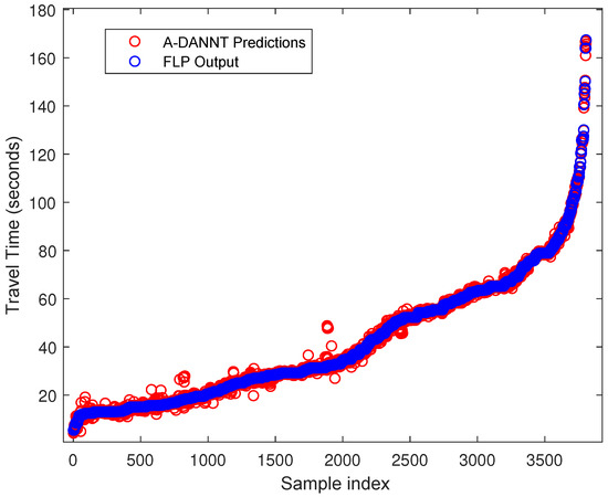
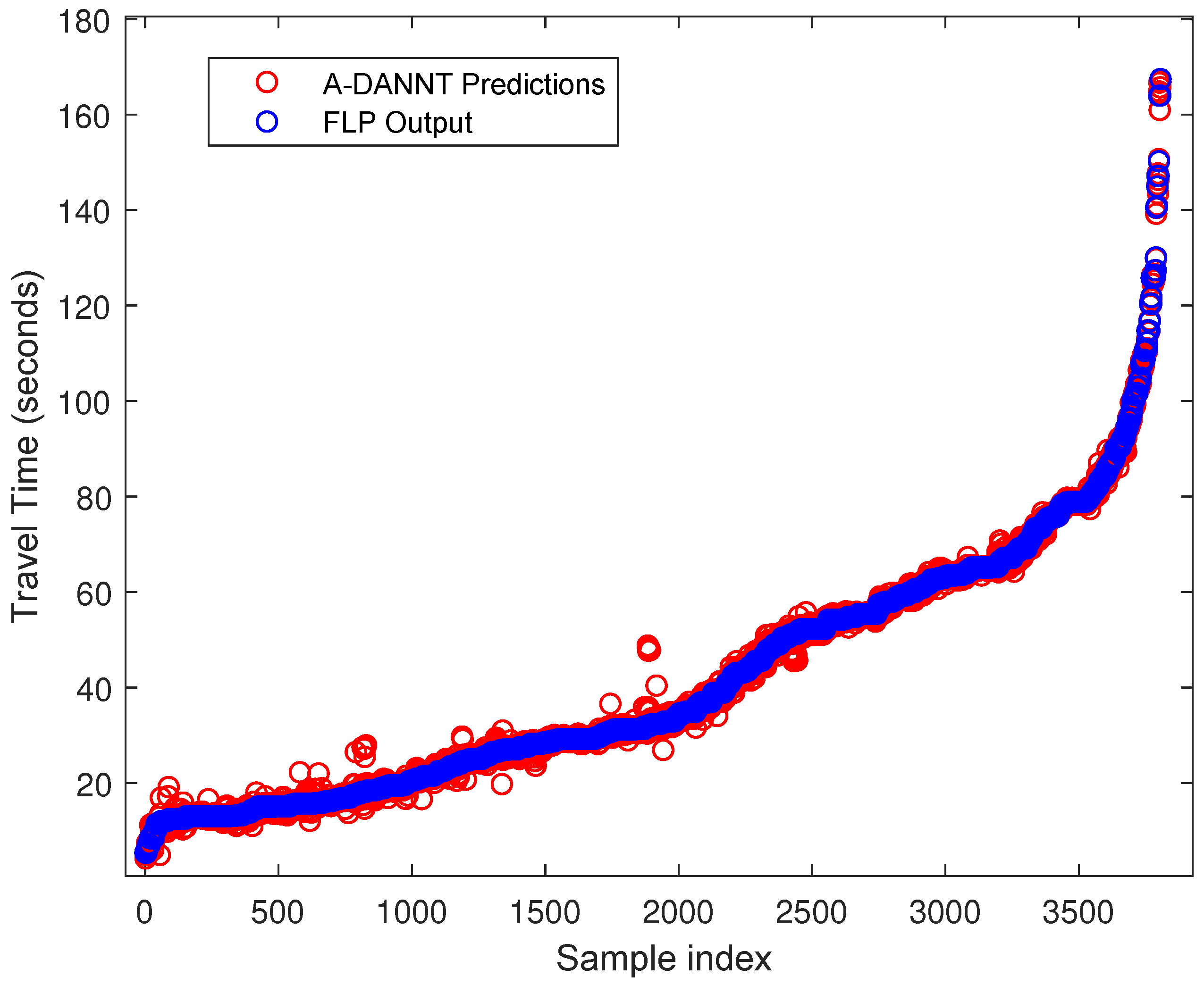
For case 2, the values estimated by the neural network are compared with the desired values, resulting in the precision of any value in the output set. In comparison with the dataset of the article in question, Figure 16 shows the desired values with the values estimated by the trained network, where MSE is 1.5312 s.

Figure 16. Comparison between A-DANNT predicted travel time and the reference FLP measurements across the full dataset.

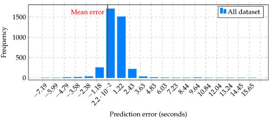
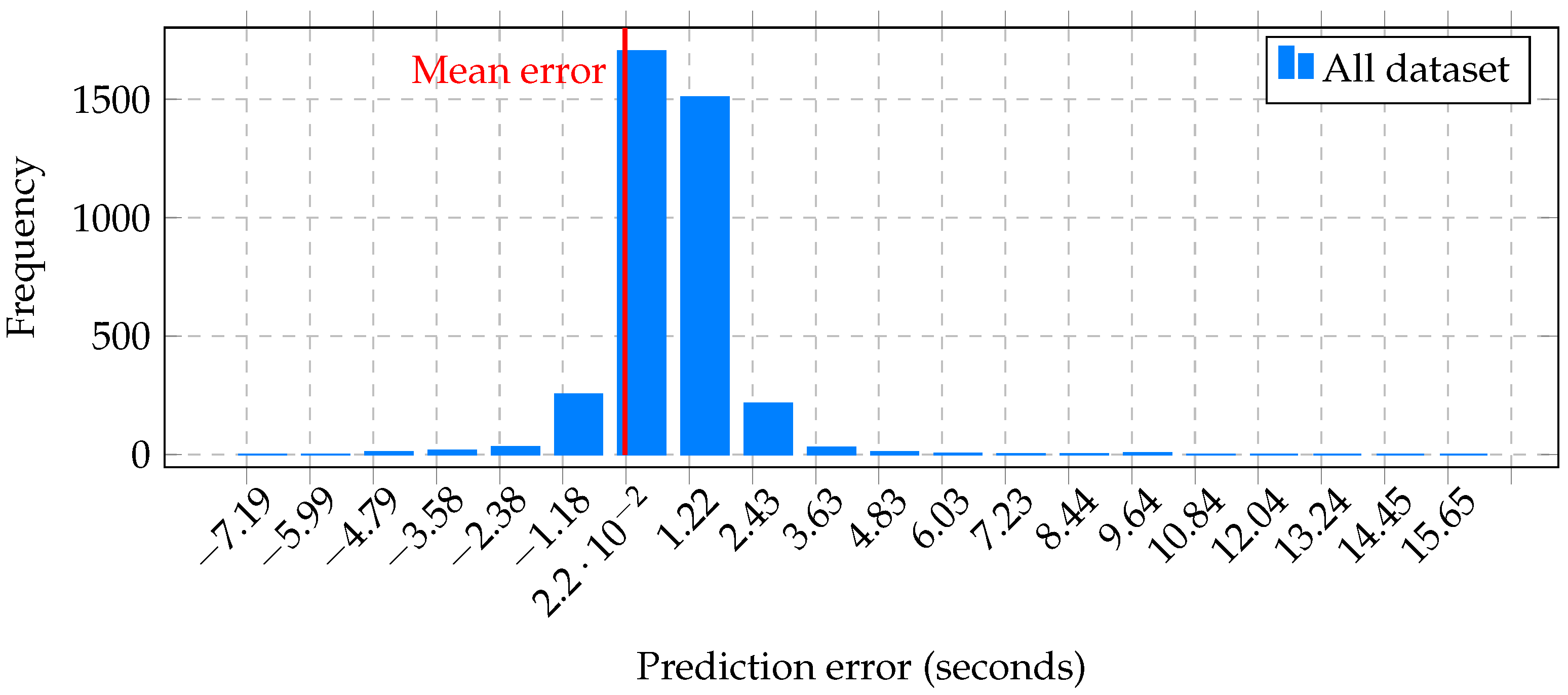
Figure 17 shows the frequency or trend of the error graphically (the desired output minus the actual output) with 20 bars; for case 2, the entire dataset observes and the red line represents the mean error.

Figure 17. Histogram of prediction errors between the FLP reference values and the A-DANNT estimates for the complete dataset.

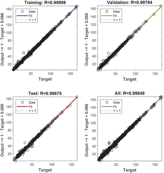
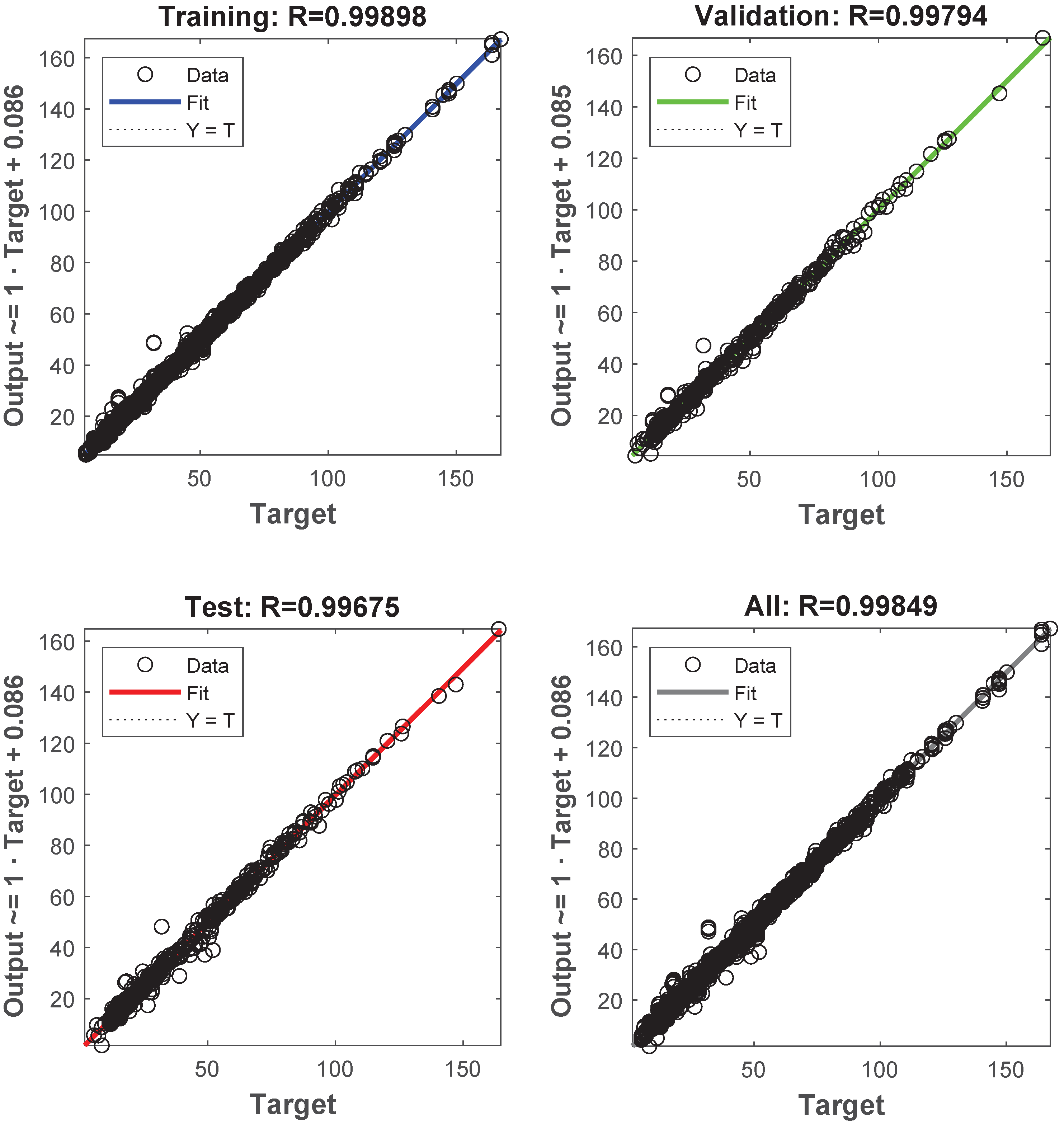
Figure 18 presents the linear regression analysis for the training, validation, test, and full datasets in Case 2. The dotted line represents the ideal relationship $outputs=targets$, and the continuous line indicates the best-fit regression between outputs and targets. The obtained correlation coefficients are $R=0.99898$ (training), $R=0.99794$ (validation), $R=0.99675$ (test), and $R=0.99849$ (all data). The consistency among the three subsets demonstrates stable predictive performance across unseen data partitions.

Figure 18. Linear regression analysis for case 2 showing training, validation, test, and full dataset performance.

To assess whether the difference between the population means is statistically significant, the significance levels of cases 1 and 2 are compared with the p-value. Usually, a significance level (denoted as $\alpha$ or alpha) of 5% works properly. The 0.05 level of significance indicates a 5% risk of concluding that the difference is statistically significant when there is no real difference, as shown in Table 10 and Table 11.

Table 10. CI and test statistic T: Target and output.

Descriptive Statistics
Sample	N	Mean	StDev	SE Mean
Target	10,000	96.051	53.163	0.532
Output	10,000	96.104	53.013	0.53
Estimation for Paired Difference
Mean	StDev	SE Mean	95% CI for ${\mathit{\mu }}_{\mathbf{difference}}$
−0.0525	4.7454	0.0475	(−0.1455, 0.0405)
${\mu }_{\mathrm{difference}}$: mean of (Target–Output)

Table 11. Test statistic T: Real and A-DANNT.

Descriptive Statistics
Sample	N	Mean	StDev	SE Mean
Target	21	5.278	2.291	0.50
Output	21	5.067	2.092	0.457
Estimation for Paired Difference
Mean	StDev	SE Mean	95% CI for ${\mathit{\mu }}_{\mathbf{difference}}$
0.211	0.501	0.109	(−0.100, 0.522)
${\mu }_{\mathrm{difference}}$: mean of (Target–Output)

Value $p>\alpha$: The difference between the means is not statistically significant ($H_0$ is not rejected).

To assess the stability of the predictions, a 95% confidence interval for the paired differences was computed. For Case Study 1, the obtained interval (−0.1455, 0.0405) indicates consistent predictive behavior of the proposed model, while for Case Study 2, the interval (−0.100, 0.522) confirms similar behavior. Additionally, a variance analysis of the Absolute Percentage Error was performed. The proposed A-DANNT model exhibited lower dispersion (32.64%) compared to the FLP model (46.57%), indicating greater stability of the predictions. The confidence interval and variance analyses support the robustness and stability of the proposed model across different scenarios.

The residual distribution was inspected to evaluate potential systematic bias in the predictions. The errors are centered around zero and remain bounded, indicating no consistent overestimation or underestimation behavior.

Furthermore, performance was analyzed across different traffic scenarios and temporal segments (peak and off-peak periods). The obtained error metrics showed comparable magnitudes across these subsets, suggesting stable predictive behavior across the operating conditions represented in the dataset.

3.3. Residual Analysis and Error Distribution

To complement the correlation coefficient R, additional evaluation was performed using $RMSE$ and $MAE$, which quantify the magnitude of prediction deviations. During the A-DANNT search, R guides the selection of candidate topologies, while RMSE and MAE are used to assess numerical prediction accuracy.

The residual distribution was inspected to verify that prediction errors remain centered and bounded without systematic bias. Most deviations are concentrated around zero with limited dispersion, indicating consistent predictive behavior across the dataset. Thus, the correlation measure provides structural consistency during topology selection, whereas RMSE and MAE provide magnitude-based validation of the final model.

3.4. Generalization and Transferability Analysis

The proposed A-DANNT framework is not inherently tied to a specific road network. Since the topology search strategy automatically determines the neural architecture according to the statistical properties of the training dataset, the model can be retrained using data from different cities or traffic scenarios without manual redesign of the network structure.

Rather than relying on a fixed architecture, the method adapts the number of layers and neurons to the complexity observed in the data. Therefore, the framework can be interpreted as a reusable modeling procedure that may be applied to different urban environments, provided that representative local training data are available.

To evaluate robustness within the available dataset, the model was tested across multiple data partitions and temporal subsets, including peak and off-peak periods. The $RMSE$ and $MAE$ values showed only minor variations between subsets, indicating that the predictive performance is not strongly dependent on a particular data segment. This behavior suggests stable performance across the traffic conditions represented in the dataset.

4. Conclusions

In conclusion, based on the paired T analysis, the p value is greater than the significance level (see Table 12 and Table 13); in cases 1 and 2, for the decision in both cases, the null hypothesis cannot be rejected. There is not enough evidence to conclude that the difference in means between the paired observations is statistically significant. Additionally, the computed 95% confidence intervals include zero, which supports the statistical consistency of the obtained results and reinforces that the observed differences are not statistically significant.

Table 12. Hypothesis test results for the paired t-test between target and output values.

Test
Null hypothesis		$H_0:{\mu }_{\mathrm{difference}}=0$
Alternative hypothesis		$H_1:{\mu }_{\mathrm{difference}}\ne 0$
T-value	p-value
−1.11	0.268

Table 13. Hypothesis test results for the paired t-test between real data and A-DANNT predictions.

Test
Null hypothesis		$H_0:{\mu }_{\mathrm{difference}}=0$
Alternative hypothesis		$H_1:{\mu }_{\mathrm{difference}}\ne 0$
T-value	p-value
−0.02	0.987

There is a relationship between the data number from the dataset, the layers, and the neurons of topology; if there is little data to analyze and many neurons, the neurons memorize the values, causing an overfit; in other words, the architecture memorizes the trained data; when generating new data, if not in the dataset, the forecast will have a more significant margin of error. In other cases, the input variables are considered dynamic over time. In this work, the variable $Ss$ (Street state) can change from no obstacle to large potholes over time and rain; these problems make it necessary to create an auto-design algorithm that automatically helps choose the correct topology for each problem; the A-DANNT algorithm reduces user error when choosing a topology and automates the choice of design.

The use of the BR-vD algorithm guarantees the obtainment of a set of weights w with a higher correlation coefficient, with this value being close to an overall maximum. Nevertheless, as the search relies on a heuristic strategy, the obtained solution corresponds to a high-quality local optimum rather than a guaranteed global optimum. The BR-vD algorithm application ensures a set of weights that fit the input values and the specific problem data. The weight set is stored in an $r_m$ variable and is iteratively compared until the set provides the best results.

A statistical test analysis helps decide if the design fits the problem, choosing a correlation coefficient with a higher R-value. The complementary confidence interval and variance analyses further demonstrate the robustness and stability of the predictive behavior across the evaluated scenarios.

For case 1, the test dataset indicates a good fit. The test dataset results also show R-values up to 0.99366. The diagram in Figure 11 is helpful to show that specific data points have poor settings. For example, there is a data point in the network output values whose value is 270.6 s, while the corresponding target value is 210.4 s with input values of Sd = 313, Ss = 24, Tz = 1, Td = 15, and Rl = 28, while the corresponding target value is 210.4 s. The next step would be to investigate this data point to determine if it represents an atypical value (i.e., if it is outside the training dataset). It should include the training package and additional data collected for the test or training package.

However, the data estimated by the network proposed to show a Mean Absolute Error of 3.2765 s and a high percentage for values with an adjustment close to zero, which shows the efficiency of the model. For example, the data point in the values of the network output, whose value is 41.2684, while the corresponding target value is 41.2688, the difference being $4\times {10}^{-4}$, corroborates the existence of the minimum error in most data.

For case 2, the output trained data RNA shows an R-value of 0.99898; the topology proposed by A-DANNT for this case specifies one input layer with 11 neurons, 150 hidden layer neurons, and one neuron output layer. Figure 16 is helpful to verify how the target dataset fits the ANN predictions, where the red circles represent the predictions of A-DANNT and the blue circles represent the FLP values. A Mean Absolute Error of 0.6957 s is obtained, where a high percentage of the values are close to zero. In the same way, a Mean Absolute Error of 0.6957 s is obtained, where a high percentage of the values are close to zero. In the same way, the MAPE comparison for the FLP and A-DANNT data is shown in Table 9, and it is concluded that the values proposed by the network better fit the target values. Overall, the proposed methodology demonstrates accurate prediction capability while maintaining statistical stability, supporting its applicability as an automatic topology design strategy for regression problems.

References

- Visser, J.; Nemoto, T.; Browne, M. Home delivery and the impacts on urban freight transport: A review. Procedia-Soc. Behav. Sci. 2014, 125, 15–27. [Google Scholar] [CrossRef] [Scilit]
- Florio, A.M.; Feillet, D.; Hartl, R.F. The delivery problem: Optimizing hit rates in e-commerce deliveries. Transp. Res. Part B Methodol. 2018, 117, 455–472. [Google Scholar] [CrossRef] [Scilit]
- Fragoso-Mandujano, J.A.; Pérez-Patricio, M.; Camas-Anzueto, J.L.; Vázquez-Delgado, H.D.; Chandomí-Castellanos, E.; Gonzalez-Baldizón, Y.; Guzman-Rabasa, J.A.; Martinez-Morgan, J.C.; Guillén-Ruíz, L.E. Towards an Approach for Filtration Efficiency Estimation of Consumer-Grade Face Masks Using Thermography. Appl. Sci. 2022, 12, 2071. [Google Scholar] [CrossRef] [Scilit]
- Hobbs, J.E. Food supply chains during the COVID-19 pandemic. Can. J. Agric. Econ. Can. D’agroeconomie 2020, 68, 171–176. [Google Scholar] [CrossRef] [Scilit]
- Gao, X.; Shi, X.; Guo, H.; Liu, Y. To buy or not buy food online: The impact of the COVID-19 epidemic on the adoption of e-commerce in China. PLoS ONE 2020, 15, e0237900. [Google Scholar] [CrossRef] [Scilit]
- Noland, R.; Small, K.A. Travel-time uncertainty, departure time choice, and the cost of morning commutes. Transp. Res. Rec. 1995, 1, 150–158. [Google Scholar]
- Wigan, M.; Rockliffe, N.; Thoresen, T.; Tsolakis, D. Valuing long-haul and metropolitan freight travel time and reliability. Transp. Stat. 2000, 1, 83–89. [Google Scholar]
- Huu, D.N.; Ngoc, V.N. Analysis Study of Current Transportation Status in Vietnam’s Urban Traffic and the Transition to Electric Two-Wheelers Mobility. Sustainability 2021, 13, 5577. [Google Scholar] [CrossRef] [Scilit]
- Liu, H.; Van Zuylen, H.; Van Lint, H.; Salomons, M. Predicting urban arterial travel time with state-space neural networks and Kalman filters. Transp. Res. Rec. 2006, 1968, 99–108. [Google Scholar] [CrossRef]
- Altinkaya, M.; Zontul, M. Urban bus arrival time prediction: A review of computational models. Int. J. Recent Technol. Eng. (IJRTE) 2013, 2, 164–169. [Google Scholar]
- Gurmu, Z.K.; Fan, W.D. Artificial neural network travel time prediction model for buses using only GPS data. J. Public Transp. 2014, 17, 3. [Google Scholar] [CrossRef] [Scilit]
- Yu, L.; Xie, B.; Chan, E.H. Exploring impacts of the built environment on transit travel: Distance, time and mode choice, for urban villages in Shenzhen, China. Transp. Res. Part E Logist. Transp. Rev. 2019, 132, 57–71. [Google Scholar] [CrossRef] [Scilit]
- Ma, J.; Chan, J.; Ristanoski, G.; Rajasegarar, S.; Leckie, C. Bus travel time prediction with real-time traffic information. Transp. Res. Part C Emerg. Technol. 2019, 105, 536–549. [Google Scholar] [CrossRef] [Scilit]
- Davidson, K. A flow travel time relationship for use in transportation planning. In Proceedings of the Australian Road Research Board (ARRB) Conference, 3rd, Sydney; The National Academies of Sciences, Engineering, and Medicine: Washington, DC, USA, 1966; Volume 3, pp. 183–194. [Google Scholar]
- Lyman, K.; Bertini, R.L. Using travel time reliability measures to improve regional transportation planning and operations. Transp. Res. Rec. 2008, 2046, 1–10. [Google Scholar] [CrossRef] [Scilit]
- Tirachini, A.; Antoniou, C. The economics of automated public transport: Effects on operator cost, travel time, fare and subsidy. Econ. Transp. 2020, 21, 100151. [Google Scholar] [CrossRef] [Scilit]
- Margulici, J.; Ban, X. Benchmarking travel time estimates. IET Intell. Transp. Syst. 2008, 2, 228–237. [Google Scholar] [CrossRef] [Scilit]
- Cebecauer, M.; Jenelius, E.; Burghout, W. Integrated framework for real-time urban network travel time prediction on sparse probe data. IET Intell. Transp. Syst. 2017, 12, 66–74. [Google Scholar] [CrossRef] [Scilit]
- Lu, L.; Wang, J.; He, Z.; Chan, C.Y. Real-time estimation of freeway travel time with recurrent congestion based on sparse detector data. IET Intell. Transp. Syst. 2017, 12, 2–11. [Google Scholar] [CrossRef] [Scilit]
- Viergutz, K.; Krajzewicz, D. Analysis of the Travel Time of Various Transportation Systems in Urban Context. Transp. Res. Procedia 2019, 41, 313–323. [Google Scholar] [CrossRef] [Scilit]
- Chang, H.; Park, D.; Lee, S.; Lee, H.; Baek, S. Dynamic multi-interval bus travel time prediction using bus transit data. Transportmetrica 2010, 6, 19–38. [Google Scholar] [CrossRef] [Scilit]
- Pirc, J.; Turk, G.; Žura, M. Highway travel time estimation using multiple data sources. IET Intell. Transp. Syst. 2016, 10, 649–657. [Google Scholar] [CrossRef] [Scilit]
- Jamous, W.; Balijepalli, C. Assessing travel time reliability implications due to roadworks on private vehicles and public transport services in urban road networks. J. Traffic Transp. Eng. (Engl. Ed.) 2018, 5, 296–308. [Google Scholar] [CrossRef] [Scilit]
- Ma, Z.; Koutsopoulos, H.N.; Ferreira, L.; Mesbah, M. Estimation of trip travel time distribution using a generalized Markov chain approach. Transp. Res. Part C Emerg. Technol. 2017, 74, 1–21. [Google Scholar] [CrossRef] [Scilit]
- Geroliminis, N.; Skabardonis, A. Identification and analysis of queue spillovers in city street networks. IEEE Trans. Intell. Transp. Syst. 2011, 12, 1107–1115. [Google Scholar] [CrossRef] [Scilit]
- Kisgyörgy, L.; Rilett, L.R. Travel time prediction by advanced neural network. Period. Polytech. Civ. Eng. 2002, 46, 15–32. [Google Scholar]
- Dharia, A.; Adeli, H. Neural network model for rapid forecasting of freeway link travel time. Eng. Appl. Artif. Intell. 2003, 16, 607–613. [Google Scholar] [CrossRef] [Scilit]
- Wu, C.H.; Ho, J.M.; Lee, D.T. Travel-time prediction with support vector regression. IEEE Trans. Intell. Transp. Syst. 2004, 5, 276–281. [Google Scholar] [CrossRef] [Scilit]
- Mark, C.D.; Sadek, A.W.; Rizzo, D. Predicting experienced travel time with neural networks: A PARAMICS simulation study. In Proceedings of the 7th International IEEE Conference on Intelligent Transportation Systems (IEEE Cat. No. 04TH8749), Washington, WA, USA, 3–6 October 2004; IEEE: Piscataway, NJ, USA, 2004; pp. 906–911. [Google Scholar]
- Van Lint, J.; Hoogendoorn, S.; van Zuylen, H.J. Accurate freeway travel time prediction with state-space neural networks under missing data. Transp. Res. Part C Emerg. Technol. 2005, 13, 347–369. [Google Scholar] [CrossRef] [Scilit]
- Jiang, Z.; Zhang, C.; Xia, Y. Travel time prediction model for urban road network based on multi-source data. Procedia-Soc. Behav. Sci. 2014, 138, 811–818. [Google Scholar] [CrossRef] [Scilit]
- Wang, J.; Tsapakis, I.; Zhong, C. A space–time delay neural network model for travel time prediction. Eng. Appl. Artif. Intell. 2016, 52, 145–160. [Google Scholar] [CrossRef] [Scilit]
- Zheng, F.; Van Zuylen, H. Uncertainty and Predictability of Urban Link Travel Time: Delay Distribution–Based Analysis. Transp. Res. Rec. 2010, 2192, 136–146. [Google Scholar] [CrossRef] [Scilit]
- Escobar-Gómez, E.; Camas-Anzueto, J.; Velázquez-Trujillo, S.; Hernandez-de Leon, H.; Grajales-Coutiño, R.; Chandomí-Castellanos, E.; Guerra-Crespo, H. A Linear Programming Model with Fuzzy Arc for Route Optimization in the Urban Road Network. Sustainability 2019, 11, 6665. [Google Scholar] [CrossRef] [Scilit]
- Ji, X. Models and algorithm for stochastic shortest path problem. Appl. Math. Comput. 2005, 170, 503–514. [Google Scholar] [CrossRef] [Scilit]
- Cheng, J.; Lisser, A.; Letournel, M. Distributionally robust stochastic shortest path problem. Electron. Notes Discret. Math. 2013, 41, 511–518. [Google Scholar] [CrossRef] [Scilit]
- van Hinsbergen, C.I.; Van Lint, J.; Van Zuylen, H. Bayesian training and committees of state-space neural networks for online travel time prediction. Transp. Res. Rec. 2009, 2105, 118–126. [Google Scholar] [CrossRef] [Scilit]
- Van Hinsbergen, C.; Hegyi, A.; Van Lint, J.; Van Zuylen, H. Bayesian neural networks for the prediction of stochastic travel times in urban networks. IET Intell. Transp. Syst. 2011, 5, 259–265. [Google Scholar] [CrossRef] [Scilit]
- Woodard, D.; Nogin, G.; Koch, P.; Racz, D.; Goldszmidt, M.; Horvitz, E. Predicting travel time reliability using mobile phone GPS data. Transp. Res. Part C Emerg. Technol. 2017, 75, 30–44. [Google Scholar] [CrossRef] [Scilit]
- Li, B. Measuring travel time reliability and risk: A nonparametric approach. Transp. Res. Part B Methodol. 2019, 130, 152–171. [Google Scholar] [CrossRef] [Scilit]
- Chen, B.Y.; Cheng, X.P.; Kwan, M.P.; Schwanen, T. Evaluating spatial accessibility to healthcare services under travel time uncertainty: A reliability-based floating catchment area approach. J. Transp. Geogr. 2020, 87, 102794. [Google Scholar] [CrossRef] [Scilit]
- Liu, D.; Kwan, M.P. Measuring job accessibility through integrating travel time, transit fare and income: A study of the Chicago metropolitan area. Tijdschr. Econ. Soc. Geogr. 2020, 111, 671–685. [Google Scholar] [CrossRef] [Scilit]
- Rupnik, J.; Davies, J.; Fortuna, B.; Duke, A.; Clarke, S.S. Travel time prediction on highways. In Proceedings of the 2015 IEEE International Conference on Computer and Information Technology; Ubiquitous Computing and Communications; Dependable, Autonomic and Secure Computing; Pervasive Intelligence and Computing, Liverpool, UK, 26–28 October 2015; IEEE: Piscataway, NJ, USA, 2015; pp. 1435–1442. [Google Scholar]
- Nikovski, D.; Nishiuma, N.; Goto, Y.; Kumazawa, H. Univariate short-term prediction of road travel times. In Proceedings of the 2005 IEEE Intelligent Transportation Systems, Vienna, Austria, 13–16 September 2005; IEEE: Piscataway, NJ, USA, 2005; pp. 1074–1079. [Google Scholar]
- Yang, J.S. Travel time prediction using the GPS test vehicle and Kalman filtering techniques. In Proceedings of the 2005 American Control Conference, Portland, OR, USA, 8–10 June 2005; IEEE: Piscataway, NJ, USA, 2005; pp. 2128–2133. [Google Scholar]
- Lee, W.H.; Tseng, S.S.; Tsai, S.H. A knowledge based real-time travel time prediction system for urban network. Expert Syst. Appl. 2009, 36, 4239–4247. [Google Scholar] [CrossRef] [Scilit]
- Çetiner, B.G.; Sari, M.; Borat, O. A neural network based traffic-flow prediction model. Math. Comput. Appl. 2010, 15, 269–278. [Google Scholar] [CrossRef] [Scilit]
- Abdollahi, M.; Khaleghi, T.; Yang, K. An integrated feature learning approach using deep learning for travel time prediction. Expert Syst. Appl. 2020, 139, 112864. [Google Scholar] [CrossRef] [Scilit]
- Smithson, S.C.; Yang, G.; Gross, W.J.; Meyer, B.H. Neural networks designing neural networks: Multi-objective hyper-parameter optimization. In Proceedings of the 35th International Conference on Computer-Aided Design, Austin, TX, USA, 7–10 November 2016; pp. 1–8. [Google Scholar]
- Boozarjomehry, R.; Svrcek, W. Automatic design of neural network structures. Comput. Chem. Eng. 2001, 25, 1075–1088. [Google Scholar] [CrossRef] [Scilit]
- Garro, B.A.; Vázquez, R.A. Designing artificial neural networks using particle swarm optimization algorithms. Comput. Intell. Neurosci. 2015, 2015, 369298. [Google Scholar] [CrossRef] [Scilit]
- Kapanova, K.; Dimov, I.; Sellier, J. A genetic approach to automatic neural network architecture optimization. Neural Comput. Appl. 2018, 29, 1481–1492. [Google Scholar] [CrossRef] [Scilit]
- Toghraie, D.; Sina, N.; Jolfaei, N.A.; Hajian, M.; Afrand, M. Designing an Artificial Neural Network (ANN) to predict the viscosity of Silver/Ethylene glycol nanofluid at different temperatures and volume fraction of nanoparticles. Phys. A Stat. Mech. Its Appl. 2019, 534, 122142. [Google Scholar] [CrossRef] [Scilit]
- Del Brío, B.M.; Molina, A.S. Redes Neuronales y Sistemas Borrosos; Ra-Ma: Madrid, Spain, 2001. [Google Scholar]
- Haykin, S. Neural Networks and Learning Machines, 3/E; Pearson Education: Noida, India, 2010. [Google Scholar]
- Beale, M.H.; Hagan, M.T.; Demuth, H.B. Neural Network Toolbox User’s Guide; MathWorks Inc.: Natick, MA, USA, 1992; Volume 1. [Google Scholar]
- Jaziri, W. Local Search Techniques: Focus on Tabu Search; TEH: Zagreb, Croatia, 2008. [Google Scholar]
- Glover, F. Tabu search—Part II. ORSA J. Comput. 1990, 2, 4–32. [Google Scholar] [CrossRef] [Scilit]
- Alba, E.; Aldana, J.; Troya, J.M. Full automatic ANN design: A genetic approach. In Proceedings of the International Workshop on Artificial Neural Networks, Sitges, Spain, 9–11 June 1993; Springer: Berlin/Heidelberg, Germany, 1993; pp. 399–404. [Google Scholar]
- Saemi, M.; Ahmadi, M.; Varjani, A.Y. Design of neural networks using genetic algorithm for the permeability estimation of the reservoir. J. Pet. Sci. Eng. 2007, 59, 97–105. [Google Scholar] [CrossRef] [Scilit]
- Vu, L.H.; Passow, B.N.; Paluszczyszyn, D.; Deka, L.; Goodyer, E. Estimation of Travel Times for Minor Roads in Urban Areas Using Sparse Travel Time Data. IEEE Intell. Transp. Syst. Mag. 2021, 13, 220–233. [Google Scholar] [CrossRef] [Scilit]
- Van Lint, J. Reliable Travel Time Prediction for Freeways; Netherlands TRAIL Research School: Delft, The Netherlands, 2004. [Google Scholar]
- Chandomí-Castellanos, E.; Escobar-Gómez, E.N.; Velázquez-Trujillo, S.; León, H.R.H.D.; Pérez-Patricio, M.; Pérez, C.V.D.C. Modelo para la determinación de la ruta más corta con funciones experimentales para arcos difusos. Res. Comput. Sci. 2019, 148, 317–330. [Google Scholar] [CrossRef] [Scilit]
Disclaimer/Publisher’s Note: The statements, opinions and data contained in all publications are solely those of the individual author(s) and contributor(s) and not of MDPI and/or the editor(s). MDPI and/or the editor(s) disclaim responsibility for any injury to people or property resulting from any ideas, methods, instructions or products referred to in the content. |
© 2026 by the authors. Licensee MDPI, Basel, Switzerland. This article is an open access article distributed under the terms and conditions of the Creative Commons Attribution (CC BY) license.