


Abstract
Daily equity return forecasting is challenging due to low signal-to-noise ratios, heavy-tailed innovations, and persistent distribution drift. We study one-step-ahead log-return prediction using daily market variables and return-based transformations. We propose a CNN–LightGBM hybrid that transfers a last-step CNN embedding to a gradient-boosted tree regressor through explicit embedding standardization, which stabilizes the representation interface for tree learning. To reduce train-to-evaluation mismatch under drift, we adopt split-wise, training-only standardization with a recency-aware fit-latest-W rule. Return-related predictors are anchored on a one-sided wavelet-denoised close series, while other market channels are retained in their original form to preserve episodic extremes. Experiments on NIFTY50 with walk-forward model selection show statistically reliable accuracy gains over Naive0 and competitive performance against representative deep sequence baselines, and the supplementary evaluations on HDFC and INDA provide additional out-of-sample evidence on these two assets under the same strictly chronological protocol. A long-or-cash decision rule based on the return forecasts yields positive risk-adjusted performance under realistic transaction-cost assumptions, supporting the practical relevance of the predictive signal.
1. Introduction
Forecasting equity movements remains a core challenge in quantitative finance [1,2]. Price dynamics are shaped by interacting drivers that range from macroeconomic policy and industry cycles to firm fundamentals, geopolitical shocks, and shifts in investor sentiment [3]. These interacting forces can create transient regularities, yet the resulting series are noisy and exhibit time-varying distributions, which makes reliable out-of-sample forecasting difficult [4].
Classical investment analysis is often organized around fundamental analysis and technical analysis [5]. Fundamental analysis evaluates intrinsic value through macro indicators, industry competition, and firm profitability [6]. Technical analysis summarizes market behavior using price–volume patterns and indicator families such as candlestick charts and moving averages [5,7]. Although widely used in practice, both approaches can be sensitive to modeling choices and to the timeliness and subjectivity of the information used [6,7].
Motivated by these limitations, a large body of work has explored statistical and machine-learning models for market prediction [8,9]. The Autoregressive Integrated Moving Average model, abbreviated as ARIMA, can be effective under approximate stationarity, but it often deteriorates when dynamics become nonlinear or regime dependent. The Generalized Autoregressive Conditional Heteroskedasticity model, abbreviated as GARCH, captures volatility clustering but can be less responsive around abrupt structural changes [10]. More recently, machine-learning models such as Support Vector Machines and Random Forests have been applied to improve predictive performance, while raising new questions regarding stability and interpretability under noisy labels [11].
Deep sequence models further expanded the modeling toolkit by learning representations directly from multi-variate histories [12]. CNN–LSTM variants are frequently used to combine local pattern extraction with temporal dependency modeling [13]. Hybrid designs that combine recurrent networks with gradient-boosted trees have also been reported in related financial tasks such as volatility forecasting [14]. In addition, wavelet-based denoising has been explored as a preprocessing component to improve the signal quality before a nonlinear predictor [15]. These studies support the view that combining complementary inductive biases can be useful in low signal-to-noise settings, provided that the experimental protocol is rigorously time-ordered [9,16]. However, many hybrid studies treat the handoff between a neural representation and a tree-based head as an implementation detail and provide limited specification on how scale stability is maintained across components. This under-specification makes it difficult to distinguish gains from an explicit representation-transfer mechanism from gains that could be reproduced by a trivial combination of standalone predictors. Our design addresses this issue by standardizing the transferred last-step embedding before tree regression and by validating the resulting gain against a simple averaging baseline and structured ablations.
Recent advances in time-series forecasting also include Transformer-style architectures [17]. Informer improves efficiency for long sequences through a sparse attention mechanism and a tailored decoding strategy [18]. TimesNet emphasizes multi-period structure by transforming one-dimensional series into richer representations and extracting patterns across frequency bands [19]. Related lines of work combine attention with feature engineering and heterogeneous inputs, including models that integrate auxiliary representations such as Time2Vec or multi-source indicator matrices [20,21]. While these architectures can be competitive, their reported gains can be sensitive to the forecasting target, the market under study, and the exact time-ordered evaluation protocol [17,22].
From the perspective of empirical forecasting, three methodological gaps remain salient [8,23]. First, inadvertent look-ahead can arise in feature construction and standardization when future statistics leak into model inputs or scaling, which can inflate backtest performance under nonstationary markets [16,24]. Second, hybrid models often emphasize architectural combination, yet the representation transfer across components is frequently under-specified, especially regarding scale stability when the downstream learner is sensitive to feature magnitude and temporal drift. Third, forecasting studies are frequently reported only through statistical accuracy metrics, whereas decision-oriented validation that maps forecasts to implementable actions is less consistently documented in the same strictly chronological setting [25].
To address these issues, we study one-step-ahead log-return prediction and propose a leakage-free CNN–LightGBM hybrid under a strictly chronological, no-look-ahead protocol. The inputs are constructed from market behavior variables and return-based transformations. To improve robustness under distribution shift, we adopt one-sided, past-only standardization performed split-wise on the training segment, together with a recency-aware fit-latest-W strategy. We also incorporate wavelet denoising on the close price when forming return-related quantities to mitigate high-frequency noise. On the modeling side, a one-sided CNN encoder maps multivariate histories to a compact last-step embedding, and an explicit embedding standardization step is applied before the LightGBM regressor. The CNN encoder is used to learn a stable representation, and LightGBM performs the final nonlinear regression on the standardized embedding. The modular coupling retains the representation power of convolutional encoders while leveraging the efficiency of gradient-boosted decision trees for nonlinear interaction modeling. To verify that the improvement is not explained by naive hybridization, we report a simple averaging baseline and structured ablations under the same strictly chronological protocol, as summarized in Section 5.3.
The main contributions of this work are summarized as follows:
- 1.
- A stability-oriented CNN–LightGBM hybrid with explicit representation transfer. We design a lightweight hybrid that couples a one-sided CNN encoder with a LightGBM regressor through a standardized last-step embedding, which stabilizes the feature interface for the downstream tree model.
- 2.
- Train-only, recency-aware standardization for temporal shift. We implement a strictly chronological preprocessing and split-wise standardization protocol that uses training-only, past-only statistics. Within this protocol, we introduce a recency-aware fit-latest-W rule that estimates scaling statistics from the most recent portion of the training segment to better track evolving market conditions.
- 3.
- Input-side robustness via one-sided wavelet denoising for return feature formation. When constructing return-based features, we replace the close price with its one-sided wavelet-denoised counterpart to mitigate high-frequency noise while preserving a past-only workflow.
- 4.
- Evidence under a strictly chronological protocol. We conduct expanding walk-forward validation and a held-out test evaluation on NIFTY50, and we further examine robustness on HDFC and INDA. Performance is assessed against Naive0 and representative learned baselines with statistical significance testing, and we report Ensemble-Avg together with a structured ablation suite to rule out a trivial averaging explanation. We also complement error-based metrics with an economic evaluation that converts return forecasts into implementable long-or-cash decisions.
Hybrid forecasting models typically combine a sequential encoder with a downstream predictor in either an end-to-end manner or a loosely coupled two-stage pipeline. Representative designs such as CNN–LSTM fuse representations within a single neural system, while recurrent-network–tree hybrids often export intermediate neural states to a boosted-tree head with limited specification of interface normalization. This distinction matters because tree learners are sensitive to feature magnitude, and scale drift can change split behavior even when the upstream representation remains qualitatively similar.
Our CNN–LightGBM makes the coupling explicit through the last-step embedding and a training-only channel-wise embedding standardization applied before LightGBM. This design turns the handoff into a fixed and reproducible interface, rather than an implicit outcome of upstream training dynamics. In addition, the recency-aware fit-latest-W scaling rule is selected together with model hyperparameters under expanding walk-forward validation, which aligns normalization choices with the same strictly chronological selection objective as the model configuration. Together with the averaging baseline and structured ablations reported in Section 5.3, this positioning clarifies that the reported gains are linked to an explicit representation-transfer mechanism rather than a superficial hybrid composition.
The remainder of this paper is organized as follows. Section 2 specifies the proposed CNN-LightGBM framework and the role of each module. Section 3 details the strictly chronological data-processing protocol, including one-sided wavelet denoising for return construction and training-only, split-wise standardization. Section 4 presents the experimental setup and the main empirical results, together with the corresponding visual diagnostics and method comparisons. Section 5 provides complementary analyses that assess robustness and interpretability, including sensitivity checks and evidence on how key design choices affect performance. Section 6 summarizes the findings and outlines directions for future work.
2. Proposed Model
This study proposes a cross-paradigm coupled temporal regression architecture that operates in tandem: a CNN-based feature encoder followed by a LightGBM predictor. The input consists of multivariate technical indicators stacked in chronological order. We apply split-wise standardization using training data only, with a fit-latest-W rule to reduce distribution drift while preserving a past-only protocol.
In the representation stage, the encoder begins with a pointwise convolution for channel mixing and to increase the embedding dimensionality, followed by BatchNorm, GELU, and SpatialDropout1D. We then stack a causal convolution (kernel size 3, dilation 1) with BatchNorm and GELU and connect it residually to the pointwise branch to form a causal residual block. For the CNN prediction head used during encoder training, we apply global average pooling and map the pooled features to an auxiliary output via a 48-unit dense layer and a linear head. The CNN is trained with mean squared error loss, using adaptive learning-rate decay and early stopping to curb overfitting.
During inference, we extract the embedding at the final time step from the convolutional feature maps and standardize it using training-set embedding statistics to remove cross-channel scale disparities.
- Formal definition of embedding standardization.
Let denote the last-step embedding extracted from the CNN convolutional feature maps at time t. Given the training segment of each split, we compute the channel-wise mean
and define the channel-wise standard deviation in component form as
Channels with near-zero variance are removed using a training-only mask. We then obtain the standardized embedding
and apply the same estimated on unchanged to the corresponding validation and test segments.
Embedding standardization is a split-wise, fixed channel-wise centering and scaling transformation, together with a training-only variance mask. Its immediate effect is to normalize the numerical scale across embedding channels, which stabilizes the feature interface for the histogram-based discretization in LightGBM. Because the same fixed transformation is applied unchanged to the validation and test segments, this step does not perform any test-time adaptation and does not use evaluation-period statistics. Any improvement therefore reflects a more stable representation-transfer interface and a reduction of simple first- and second-moment mismatch between training and evaluation embeddings, rather than an adaptive regime-tracking mechanism.
On the one hand, the training objective of CNN is to minimize the prediction error, which does not constrain the output embedding to have a consistent numerical range across all channels. Therefore, significant scale discrepancies often exist among different channels, and a slight global level drift may occur over time. On the other hand, LightGBM adopts histogram-based discretization and approximate split search, where the valid candidate split points with limited samples are directly related to the numerical distribution observed in the training segment. When the scale discrepancies of embedding channels are excessively large or the distribution drifts over time, the discretization process will alter the downstream split selection and regularization behavior, thus introducing unnecessary interface sensitivity.
This embedding is then fed to a LightGBM regressor with loss, and early stopping is triggered based on the validation MSE.
For hyperparameter optimization, we employ Optuna’s TPE to jointly search the fit-latest-W window W (WIN), the sequence look-back length L (LOOKBACK), the CNN learning rate (LR), and key LightGBM hyperparameters. The optimization objective is a time-weighted walk-forward OOS- against the strong baseline Naive0, assigning larger weights to later validation folds to better match the test-set distribution. During training, we reserve a trailing slice of the training data as an internal validation set for CNN early stopping and for visualizing training dynamics, while the test set remains isolated throughout to ensure an objective assessment of out-of-sample performance.
By combining the CNNs ability to hierarchically extract temporal patterns with LightGBMs capacity to model complex, non-linear feature interactions, the resulting architecture exhibits stable out-of-sample performance under temporal evolution and distribution shift in our evaluated setting. Figure 1 and Figure 2 show the simplified overview of the research framework and the collaborative architecture details of CNN-LightGBM, respectively.
Figure 1.
Diagrammatic illustration of the proposed research plan.
Figure 2.
CNN–LightGBM hybrid framework. BN denotes batch normalization. GELU denotes the Gaussian error linear unit. SDrop1D denotes one-dimensional spatial dropout. k and d denote kernel size and dilation rate, respectively. GAP denotes global average pooling. FC denotes a fully connected layer and 48 is the number of units. Train mean/std indicates embedding standardization using the training-set mean and standard deviation. MSE denotes mean squared error and L2 loss. Val MSE indicates that early stopping monitors the validation-set MSE. Feature sampling denotes LightGBM column subsampling. fit-latest-W denotes recency-aware, training-only standardization.
2.1. Convolutional Neural Network
The forecasting target is the next-day log return, and the predictive signal is weak relative to observation noise. In this regime, a compact encoder with a strong locality bias is attractive because it emphasizes short-horizon temporal motifs while limiting unnecessary capacity. We therefore use a one-sided temporal CNN to summarize the lookback window into a last-step embedding, and we delegate regime-dependent nonlinearities and cross-feature interactions to LightGBM. The empirical section evaluates LSTM-LightGBM and TimesNet under the same strictly chronological protocol, which provides an explicit comparison against recurrent and modern long-sequence alternatives.
- One-sided temporal convolution and the no-look-ahead property.
Let denote the chronological lookback input at time t. We apply a one-dimensional one-sided convolution with kernel size and dilation . For a relative index , the pre-activation output is
where are trainable weights and the convolution uses no bias term. The activated feature is then computed by batch normalization followed by GELU,
In implementation, one-sided left padding with zeros is applied so that the output length remains L. As a result, depends only on and never uses any input beyond the current index, which enforces the no-look-ahead property within the lookback window.
- Encoder template and transferred embedding.
The encoder begins with a pointwise convolution that mixes channels and maps inputs to an embedding dimension of . This layer is followed by batch normalization, GELU, and one-dimensional spatial dropout with rate . Next, we apply the one-sided convolution in Equation (4) and add it residually to the pointwise branch. A second one-dimensional spatial dropout with rate is applied after the residual addition. This produces a sequence of feature maps of length L. The representation transferred to LightGBM is the last-step embedding extracted at the final index of the one-sided convolution feature map sequence.
During CNN training, we attach a lightweight regression head to provide a supervised signal. The head applies global average pooling over the feature map sequence, followed by a fully connected layer with 48 units and GELU activation, and a linear output trained with the mean squared error loss. For the proposed hybrid model, the final forecast is produced by LightGBM using the transferred and standardized embeddings. The CNN encoder specification is summarized in Table 1.
Table 1.
CNN encoder specification.
2.2. Light Gradient Boosting Machine
LightGBM, an optimized gradient boosting framework, was developed with a focus on both efficiency and accuracy [26]. It addresses the need for a machine learning algorithm that can handle large-scale datasets with high-dimensional features more effectively than traditional gradient boosting methods [27,28].
The architecture of LightGBM is built upon several key innovations that enhance its performance. One of these is the histogram-based decision tree algorithm, which discretizes continuous features into histograms, thereby reducing both storage requirements and computational complexity. Another notable technique is Gradient-based One-Side Sampling (GOSS) [29,30], which optimizes the sampling process during training by focusing on instances with larger gradients. LightGBM also employs Exclusive Feature Bundling (EFB) [31,32], a method that bundles infrequent features together to further improve training efficiency.
LightGBM’s computation follows an iterative process of constructing decision trees. At each step, a new tree is added to the ensemble to correct the errors of the previous trees. This iterative process can be summarized as follows:
where represents the updated prediction model after adding the t-th tree, is the previous model, is the new tree, and is a regularization parameter.
During tree construction, LightGBM adopts a leaf-wise growth strategy that selects, at each step, the leaf whose split yields the largest reduction in the objective function. Together with its histogram-based feature discretization and efficient sampling schemes, this design allows LightGBM to train high-accuracy models with lower computational cost and faster convergence than many conventional gradient boosting implementations [33].
In addition, LightGBM offers native support for parallel and distributed training, which allows it to scale effectively to large datasets and high-dimensional feature spaces. Overfitting is controlled through several regularization mechanisms, so that the learned model maintains strong predictive performance on unseen data. Taken together, these characteristics make LightGBM particularly suitable for machine learning tasks that involve large and structurally complex datasets [34,35].
In the iterative process of the eXtreme Gradient Boosting (XGBoost) algorithm, a level-wise leaf growth strategy is employed, where all leaf nodes at the same hierarchical level are split simultaneously, as illustrated in Figure 3a. However, this approach fails to differentiate the quality of leaves within the same level, forcing splits even on leaves with low gain values, which introduces substantial unnecessary computational overhead [36,37]. To address this, LightGBM implements a more efficient leaf-wise strategy. It iteratively selects the leaf with the highest splitting gain from all current leaves for division, cycling through this process (see Figure 3b). Compared to the level-wise approach, the leaf-wise method achieves greater error reduction and improved accuracy under the same number of splits [38,39]. Nevertheless, its potential drawback lies in generating deeper decision trees that may lead to overfitting. Therefore, LightGBM incorporates a maximum depth constraint to maintain efficiency while effectively mitigating overfitting risks [40].
Figure 3.
Level -wise and leaf-wise tree growth [41].
3. Dataset Preparation
This section describes the data source and forecasting target, then reports stationarity diagnostics for the return series. It further details feature construction from price and trading activity, including denoising on the close price. Finally, it presents the leakage-free standardization and sequence construction used by the CNN–LightGBM pipeline, and summarizes all model inputs. The model is trained in the standardized domain and predictions are transformed back to the log-return domain for evaluation.
3.1. Data, Target, and Stationarity Tests
The empirical analysis uses the NIFTY 50 index with daily observations from January 2013 to December 2023. This period covers multiple market regimes, including the COVID-19 shock starting in 2020. We denote the open, high, low, and close prices by , , , and . Trading volume is denoted by , and transaction value, or turnover, is denoted by .
3.1.1. Forecasting Target (Log-Return)
Rather than modeling the non-stationary price level directly, we formulate the prediction task as one-step-ahead log-return forecasting. The supervised target is defined as
where represents the next-day log-return. The main experiments focus on the one-day horizon ().
3.1.2. Stationarity Diagnostics
To justify forecasting in the return domain, we conduct complementary stationarity tests on the price level (Close) and the one-day log-return series. Specifically, we apply the Augmented Dickey–Fuller (ADF) test, where the null hypothesis is the presence of a unit root (non-stationarity), and the KPSS test, where the null hypothesis is level stationarity. Table 2 shows that the Close series fails to reject the unit-root null under ADF () and rejects the stationarity null under KPSS (), indicating non-stationarity. In contrast, the log-return series strongly rejects the unit-root null under ADF () and does not reject stationarity under KPSS (), indicating stationarity. These results align with the standard view that return forecasting removes the common trend in price levels and forces the model to learn market dynamics rather than the price scale. Accordingly, our task is formulated as next-day log-return prediction, .
Table 2.
ADF and KPSS stationarity test results for the Close series and log returns.
3.2. Feature Construction and Denoising
3.2.1. Feature Set for Next-Day Log-Return Forecasting
Based on the daily OHLCV records and transaction value (turnover), we construct a set of price- and volume-driven predictors tailored to one-step-ahead log-return forecasting. To reduce scale effects and improve numerical stability, we apply transformations to trading activity, i.e., and . To encode intraday price geometry in a scale-invariant manner, we further form relative log-price differences from , including the log-range , the close-to-extrema gaps and , and the open-to-close change . Finally, we include return-dynamics proxies computed from the close series, namely the current log return
together with and as volatility proxies, which help distinguish low- and high-volatility regimes.
All predictors are computed using information available up to time t only. In particular, no quantities involving are used in feature construction. Therefore, the feature set does not introduce target leakage, and the evaluation strictly reflects out-of-sample forecasting of .
3.2.2. Leakage-Free One-Sided Wavelet Denoising of the Close Price
Financial close prices often contain microstructure noise and short-lived fluctuations. These high-frequency components can destabilize return-based predictors that are computed from the close series, especially when the forecasting target is the next-day log return. To improve robustness while strictly avoiding look-ahead bias, we apply a one-sided, past-only wavelet denoising procedure to the close price and denote the resulting series as .
To avoid notation ambiguity, we denote the denoising window length by and reserve L for the sequence look-back length used in sample construction. The denoising is implemented using a sliding historical window. For each time t, we form a window of length using only past and present observations, namely . Any missing values inside the window are imputed using only values within the same window, first by forward filling from earlier to later timestamps, then by a backward fill confined to the window. This step does not introduce future information beyond time t.
Given the windowed series, we perform a discrete wavelet transform and apply soft-thresholding to the detail coefficients. In the configuration selected in this study, we adopt a Daubechies wavelet of order four and determine thresholds using the BayesShrink rule. The threshold is determined by the BayesShrink rule, where both the noise level and the signal variance are estimated from the current historical window only.
Let d denote the finest-scale detail coefficients in the window. The noise standard deviation is estimated by the robust median estimator
Let be the empirical variance of the detail coefficients at a given scale. The underlying signal variance is then estimated as
The BayesShrink threshold for that scale is set to
where is a small constant to avoid numerical instability.
We then apply soft-thresholding to each detail coefficient w as
After thresholding, we reconstruct the denoised window via the inverse wavelet transform and take the last reconstructed value as the denoised estimate at time t. Since all computations are confined to , the denoising is one-sided and does not introduce any look-ahead information.
This yields the one-sided mapping
where denotes soft-thresholding and the subscript t indicates selecting the reconstructed value aligned with the current timestamp.
Within each length- window, the discrete wavelet transform is computed with symmetric boundary extension to mitigate endpoint artifacts. The decomposition depth is determined by the window length together with the chosen wavelet filter length, which ensures that the multiscale representation is well-defined within each window. Thresholding is applied scale-wise using window-local coefficient statistics as specified in Equations (9)–(11) and Equation (12). After inverse transformation, we define as the reconstructed value aligned with the current timestamp, which corresponds to the last sample of the reconstructed window. This last-sample extraction ensures that the output at time t depends only on .
Since the procedure uses only information up to time t, it remains leakage-free by construction. In addition, denoising is performed separately on chronologically split training and testing segments, so that no cross-segment information can flow through preprocessing.
In this study, wavelet denoising is applied to the close price only. First, the close price is the anchor used to build return quantities such as and the target , as well as several log-difference features. Stabilizing the close therefore stabilizes the entire return feature stack. Second, the high and low prices and trading activity often contain informative spikes reflecting sentiment and intraday volatility. Denoising these variables risks removing economically meaningful signals. This scope choice is evaluated empirically in the ablation study by adding the DenoiseHL variant, which extends the same one-sided denoising to the high and low prices while keeping all other steps unchanged. The comparison isolates whether smoothing extrema-related channels helps or hurts the out-of-sample performance.
Hyperparameter sensitivity and training-only selection. We treat the wavelet basis, threshold rule, thresholding mode, and the window length as preprocessing hyperparameters and select them within the training period only. Using the same expanding walk-forward validation protocol as in the main experiments, we evaluate a grid spanning wavelet families coif1, db2, db4, and sym4, threshold rules BayesShrink, VisuShrink, and SURE, thresholding modes soft and hard, and window lengths . For each configuration, we rerun the full forecasting workflow while keeping the remaining strictly chronological preprocessing and model training protocol unchanged, and we select the configuration that maximizes aggregated validation . Figure 4 summarizes the sensitivity patterns. Validation performance peaks at an intermediate window length, and the selected configuration uses the db4 wavelet with BayesShrink and soft thresholding at . Shorter windows retain high-frequency noise, while longer windows oversmooth the close series and weaken return-based predictors.
Figure 4.
Wavelet sensitivity.
3.3. Leakage-Free Standardization and Sequence Construction
This section specifies a chronology-preserving preprocessing protocol for one-step-ahead log-return forecasting. We first construct lookback sequences of length L and define strict boundary rules so that every sample is well-defined. We then introduce a split-wise, leakage-free standardization that is fitted using the training segment only and applied unchanged to the corresponding validation segment. A separate hold-out test set is reserved for the final evaluation and never participates in fitting standardization parameters or early stopping. To reduce sensitivity to regime changes, we use a recency-aware fit-latest-W rule for training-only standardization. The model is optimized in the standardized domain for stable learning, and all reported metrics are computed after inverse transformation in the original log-return domain.
3.3.1. Motivation and Notation
Our forecasting target is the next-day log return defined in Equation (7). At each time t, we form a p-dimensional feature vector . To capture short-horizon temporal dependence, we use a fixed lookback length L and construct a sequence input
paired with the label . For numerical conditioning, the learning objective is defined in a standardized space. For interpretability, predictions are mapped back to the original log-return space before evaluation.
3.3.2. Lookback Sequence Construction and Boundary Handling
Given the feature matrix and the next-day target, we generate supervised samples by sliding a lookback window of length L along the timeline. A sample at time t is included only when the label is available and all feature values within the lookback window are finite. This discards the first timestamps that do not admit a full lookback window, and it also discards the last timestamp where cannot be formed. The resulting dataset is a tensor of shape paired with a target vector of length N.
To preserve strict chronology, splits are performed on the sequence indices. Within the training set, we form a train–validation split by time order. In walk-forward evaluation, each fold defines its own train–validation split. The hold-out test set is used only for the final evaluation.
3.3.3. Train-Only Fit-Latest-W Standardization with Sequence-Flattened Statistics
Standardization is fitted using training data only. Split-wise standardization plays two distinct roles in our strictly chronological pipeline. It improves numerical conditioning and ensures that models operate on a comparable scale under training-only statistics. At the same time, because market-behavior variables evolve over time, statistics estimated from the entire training history can be misaligned with later periods. The fit-latest-W rule addresses this mismatch by estimating the mean and standard deviation from the most recent W training windows of each split, and then reusing the resulting fixed transformation throughout the evaluation of that split. This design reduces first- and second-moment mismatch without introducing look-ahead, since no information from the evaluation period is used when fitting the scaling parameters. We treat W as a tunable hyperparameter and select it by walk-forward validation within the training data of each split.
The fit-latest-W rule can be interpreted as a recency-aware stationarization step that reduces train-to-evaluation mismatch in the first two moments of each input dimension. However, it is not an online adaptation mechanism, because the scaling parameters are computed once from training sequences and are then kept fixed for the corresponding validation and test segments. It also does not infer a latent regime variable and does not switch model parameters or forecast rules during evaluation. This differs from explicit regime-switching formulations, which introduce a latent state process and allow parameters or decision rules to change with the inferred state. In contrast, our predictor remains unchanged, and only the training-only scaling window length is selected and then fixed within each split.
In each split, let and denote the training sequences and labels. We select the most recent W training sequences and denote their index set by .
Feature statistics are estimated after flattening the time dimension within the selected sequences. This pooling produces feature observations per dimension. For each feature dimension , we compute
If is non-finite or extremely small, we set it to 1 to avoid unstable scaling. Feature standardization is applied to every time step as
where is a small constant.
We standardize the supervised target in the same split-wise, train-only manner. Using the labels associated with , we compute
and form the standardized label
If is non-finite or extremely small, we set it to 1. The model is trained to predict . After inference, predictions are transformed back to the original log-return domain via
All forecasting metrics are computed using and in the original domain.
The transform is fixed within a split and is not refit on validation or test data.
3.4. Summary of Inputs
Table 3 reports the final set of input variables used in our forecasting pipeline, and it provides a unified view of their definitions and construction so that the information available to the model is explicit and reproducible across all splits.
Table 3.
Summary of input variables (original domain) before leakage-free standardization.
4. Experiment and Findings
This section reports the experimental setup and the main out-of-sample results for next-day log-return forecasting on NIFTY50. For a coarse view of market regimes over the sample period, Figure 5 plots the closing price together with the 50-day and 200-day moving averages, and it helps contextualize periods of pronounced trends or stress that may affect forecasting difficulty.
Figure 5.
Closing price and moving averages of NIFTY 50.
4.1. Experimental Setup
We forecast the one-step-ahead daily log return . At each time t, a p-dimensional feature vector is constructed from market variables, and a fixed lookback length L is used to form a sequence input with label . All experiments preserve strict chronology: earlier observations are used for model development and later observations are reserved for evaluation.
4.1.1. Chronological Hold-Out Split
After ordering samples chronologically, we adopt a fixed hold-out protocol: the earlier period ( of the series) is used as the training period, and the later period (the remaining ) is used as an independent test period. The test set is kept strictly untouched during model selection and is used only for reporting out-of-sample performance.
4.1.2. Compared Methods and Rationale
We adopt two standard financial benchmarks as reference points. Naive0 predicts . Persist predicts . Naive0 serves as the primary reference baseline for the main empirical conclusions in this study. It represents the no-predictability null in the daily return domain and provides a stringent yardstick because one-step log returns are tightly centered near zero. Persist is reported as a complementary benchmark that reflects a common last-observation heuristic and situates the results relative to a simple time-series rule. Reporting both benchmarks separates improvements over the zero-return null from improvements over a last-return heuristic and reduces dependence on any single baseline choice.
To isolate the contribution of each stage in the proposed pipeline, we include two component baselines: LightGBM (removing the CNN encoder) and CNN (removing the LightGBM stage and using a direct regression head).
To represent a strong hybrid recurrent baseline, we choose LSTM–LightGBM. This model follows the same two-stage philosophy as our approach—learning a sequence representation and then applying a tree-based regressor—but replaces the convolutional encoder with an LSTM. It therefore provides a direct baseline to assess whether the proposed CNN encoder yields additional predictive value beyond a recurrent encoder under the same downstream learner.
For a cross-paradigm state-of-the-art comparison, we choose TimesNet. TimesNet is a representative modern time-series forecaster that models temporal patterns in a fundamentally different manner from CNN/RNN hybrids and has shown competitive performance across diverse forecasting benchmarks. Including TimesNet allows us to position the proposed hybrid model relative to a strong long-sequence method while keeping the comparison set compact and avoiding redundant variants. All models are trained and evaluated under the same chronological protocol and the same leakage-free preprocessing procedure to ensure fairness, and they are tuned under an identical hyperparameter-selection protocol with the same optimization budget.
4.1.3. Hyperparameter Selection and Training Protocol
Hyperparameters are selected using training data only via an expanding-window walk-forward validation procedure. In each fold, the model is fitted on an expanding training prefix and evaluated on the subsequent chronological validation block; fold scores are aggregated to select the best configuration. Within each fold, a validation tail split is additionally carved out from the fold-specific training data to drive early stopping of the CNN encoder, while the external validation block is used for scoring and for early stopping of LightGBM. After fixing the best configuration, we refit the final model on the full training period and report its out-of-sample performance on the independent hold-out test set.
4.1.4. Metrics and Statistical Significance
We report RMSE, MAE, and in the original log-return domain. To quantify improvement over benchmarks, we additionally report the out-of-sample :
where the benchmark forecast is Naive0 or Persist.
Unless stated otherwise, the primary OOS- comparisons and the main conclusions are anchored to Naive0. Persist-based OOS- results are reported as a secondary reference to provide an additional benchmark that is standard in forecasting practice.
Statistical significance is assessed using the Diebold–Mariano test on the out-of-sample loss differential series under squared-error loss.
4.2. Main Results on NIFTY50
This section presents the primary test-set results for one-step-ahead log-return forecasting on NIFTY50 under a dual-baseline evaluation policy. Naive0 is the primary reference baseline for the main conclusions and significance statements. Persist is reported in parallel as a secondary benchmark to provide additional context relative to a simple last-return heuristic. We compare the proposed hybrid model CNN-LightGBM with four competitive alternatives, namely CNN, LightGBM, LSTM-LightGBM, and TimesNet. All metrics are computed on the same held-out test window with strictly aligned timestamps across methods.
4.2.1. Overall Test-Set Performance
Table 4 reports standard error metrics, including RMSE, MAE, and . It also reports out-of-sample performance measured by OOS-.
Table 4.
Main results on NIFTY50 with one-sided DM t-tests.
Daily returns exhibit a low signal-to-noise ratio, so the absolute values are expected to be small. Relative performance against strong baselines therefore provides a more informative perspective.
Across all candidates, CNN-LightGBM achieves the best overall accuracy on the test set. It attains the lowest RMSE of 0.008334. It attains the lowest MAE of 0.005890. It attains the highest of 0.027722. CNN-LightGBM also delivers the largest MSFE reduction relative to Persist. OOS- relative to Persist reaches 0.403372, which indicates a substantial improvement over the last-return heuristic. Gains over Naive0 are inherently harder because daily log-returns concentrate tightly around zero. CNN-LightGBM remains positive against Naive0 with OOS- equal to 0.028505, whereas some alternatives do not consistently outperform the zero forecast.
4.2.2. Statistical Significance: Diebold–Mariano Tests
This subsection reports statistical significance using one-sided Diebold–Mariano tests on the aligned test set. All DM tests use squared-error loss. The alternative hypothesis states that the model has smaller expected loss than the baseline under comparison.
We report the DM t-statistic computed from the out-of-sample loss differential series. A negative DM statistic indicates that the model attains a lower average squared loss than the corresponding benchmark.
Table 4 reports the baseline comparisons. Relative to Persist, every learning-based model achieves statistically significant loss reductions at the 1% level. This finding indicates that each method delivers incremental gains over the last-return rule within the adopted protocol. By contrast, Naive0 constitutes a substantially more stringent benchmark for daily returns. CNN-LightGBM exhibits a significant improvement over Naive0 at the 1% level. LightGBM provides weaker evidence in the same direction and reaches the 10% level. For the remaining alternatives, the one-sided DM tests do not reject equal predictive accuracy against the zero forecast.
We next conduct direct pairwise comparisons between CNN-LightGBM and each competing model. Table 5 shows that CNN-LightGBM attains a lower loss than every alternative with significance at the 1% level. Taken together, these results support the robustness of the hybrid design that combines representation learning with gradient boosting.
Table 5.
Pairwise DM tests.
4.2.3. Return-Level Diagnostic Visualizations
Beyond scalar scores, we provide diagnostic visualizations to characterize the association between predicted and realized returns. We also examine the temporal structure of residuals. These plots serve as model diagnostics to verify coherent behavior and to assess potential bias or drift.
True–Predicted Scatter
Figure 6, Figure 7, Figure 8, Figure 9 and Figure 10 present scatter plots of predicted returns against realized returns . The point clouds concentrate near zero, which reflects the empirical distribution of daily log-returns where large moves are infrequent. As a result, gains over Naive0 are typically modest.
Figure 6.
Scatter diagnostics: CNN.
Figure 7.
Scatter diagnostics: LightGBM.
Figure 8.
Scatter diagnostics: LSTM-LightGBM.
Figure 9.
Scatter diagnostics: TimesNet.
Figure 10.
Scatter diagnostics: CNN-LightGBM.
Despite this concentration, the scatter diagnostics still reveal meaningful differences across models. CNN-LightGBM displays a clearer monotone association between predictions and realizations, with points more aligned along the diagonal direction rather than collapsing into an undifferentiated cluster. It also shows fewer pronounced outliers, indicating improved control of large errors under squared loss. In the tails where realized returns deviate further from zero, CNN-LightGBM more consistently tracks the sign and magnitude of these moves, which contributes to its lower aggregate loss and its statistically significant advantages reported in Table 4 and Table 5.
Residual Dynamics and Rolling Bias
Figure 11, Figure 12, Figure 13, Figure 14 and Figure 15 plot residuals over time. The horizontal zero line indicates an unbiased error center. Rolling-mean overlays at 20 trading days and 60 trading days summarize short-horizon and medium-horizon bias.
Figure 11.
Residual diagnostics: CNN.
Figure 12.
Residual diagnostics: LightGBM.
Figure 13.
Residual diagnostics: LSTM-LightGBM.
Figure 14.
Residual diagnostics: TimesNet.
Figure 15.
Residual diagnostics: CNN-LightGBM.
Residuals across all models fluctuate around zero and exhibit intermittent spikes during turbulent periods. This pattern is consistent with heavy-tailed return shocks and time-varying volatility in daily log-returns. The rolling means provide a diagnostic for systematic drift. Sustained departures from zero would indicate regime-dependent miscalibration, such as persistent underprediction during rallies or overprediction during drawdowns.
CNN-LightGBM shows the most stable residual center among the candidates. Its 20-day and 60-day rolling means remain closer to zero for longer stretches, which indicates reduced bias accumulation across regimes. It also exhibits fewer extended runs of same-sign residuals, which suggests better tracking of local dynamics rather than lagging the return process. When large residual spikes occur, they tend to coincide with market-wide volatility bursts that are difficult for any model to anticipate, yet CNN-LightGBM shows faster reversion of the rolling mean toward zero after such episodes. These diagnostics support its lower aggregate loss and are consistent with the statistically significant DM advantages reported in Table 4 and Table 5.
4.2.4. Behavior During Extreme Volatility Events
Periods of elevated volatility are typically associated with heavier tails and larger absolute return moves, which can amplify forecast errors for any return-prediction model. To make the stress-period behavior explicit, we report an event-window evaluation on the held-out test window, where extreme-volatility events are defined using a training-calibrated volatility threshold and an episode-based windowing scheme.
Training-Calibrated Volatility Proxy
Let denote the one-day log return. We compute an annualized 20-day realized-volatility proxy using only the most recent 20 observed returns,
To avoid using any test-period distributional information when defining stress conditions, we set a fixed threshold as the 90th percentile of computed over the training period only. A test timestamp t is labeled as a core stress day when and as a core non-stress day otherwise.
Event-Window Construction
We construct extreme-volatility events by expanding each core episode by K trading days on both sides and taking the union of the resulting windows. We set . This procedure yields two event windows. The first event window spans 31 January 2022 to 18 April 2022 and contains 52 days. The second event window spans 7 June 2022 to 8 July 2022 and contains 24 days. In total, the event-window subset contains 76 timestamps and the complementary non-event subset contains 429 timestamps.
Stratified Performance on Event Versus Non-Event Windows
Table 6 reports performance separately on the event-window subset and on the non-event subset. For each subset, we report RMSE and MAE in the original log-return domain. We also report MSFE-based OOS-R2 relative to Naive0 computed within the same subset, so the comparison remains aligned to the same timestamps. Finally, we run one-sided DM tests against Naive0 within each subset.
Table 6.
Event-window performance.
The event-window subset exhibits larger absolute errors than the non-event subset, which is consistent with elevated volatility increasing the intrinsic difficulty of short-horizon return forecasting. At the same time, CNN-LightGBM retains a positive OOS-R2 relative to Naive0 on the event-window subset, and the DM evidence remains supportive at the 10% level. On the non-event subset, the relative gain remains positive and the DM evidence is stronger.
Overall, the event-window analysis indicates that the predictive edge of CNN-LightGBM does not vanish under extreme volatility. Although absolute errors increase during stress episodes, the model continues to deliver a positive OOS-R2 improvement over Naive0 on the event window, with supportive DM evidence at the 10% level. The same direction is observed on non-event days, where the statistical evidence is stronger.
4.3. Robustness on Additional Equities
We report supplementary out-of-sample results on two additional assets, HDFC and INDA, by applying the same preprocessing, leakage-free standardization, and training protocol used in the main experiments. HDFC provides an additional single-equity test case, while INDA is an ETF proxy for the Indian equity market. The point metrics are reported below together with OOS R2 against Naive0 and Persist, and they also include one-sided DM tests against each baseline. The pairwise DM comparisons of CNN-LightGBM against other learned models are also reported below, which directly tests whether the main model remains competitive beyond baseline-relative gains.
On HDFC, CNN-LightGBM attains the lowest RMSE at 0.015968 and the highest R2 at 0.016370 among the learned models in Table 7. The tree-based baselines are close in absolute error, with RMSE values of 0.016060 for LightGBM and 0.016058 for LSTM-LightGBM, while the standalone CNN and TimesNet are clearly less accurate and exhibit negative values. The main model also delivers the largest baseline-relative improvements, with OOS of 0.016771 versus Naive0 and 0.371645 versus Persist, exceeding the corresponding gains of LightGBM and LSTM-LightGBM. The improvement versus Naive0 is supported by a significant one-sided DM result, and the improvement versus Persist is also significant. Pairwise DM tests in Table 8 show statistically significant loss reductions versus CNN and TimesNet, while the gaps versus LightGBM and LSTM-LightGBM are not significant, which indicates that CNN-LightGBM is competitive with the strongest non-hybrid baselines on this asset. Overall, on HDFC CNN-LightGBM achieves the lowest RMSE and the highest among the learned models, and it attains statistically supported gains versus Naive0, which provides additional out-of-sample evidence on this asset under the same leakage-free protocol.
Table 7.
Robustness: HDFC.
Table 8.
DM tests: HDFC.
On INDA, CNN-LightGBM again achieves the lowest RMSE at 0.009217 and the highest at 0.027001 among the learned models in Table 9. The closest competitor on this asset is LSTM-LightGBM, which attains RMSE 0.009290 and 0.011221, while CNN remains near the benchmark level and yields a slightly negative . The main model produces the largest improvement versus Naive0, with OOS equal to 0.027006, and the one-sided DM test against Naive0 is significant at the 1% level. All learned models outperform Persist on INDA, which leads to uniformly significant Persist-based DM results and makes the Persist comparison less discriminative for ranking learned models. Pairwise DM tests in Table 10 provide a sharper comparison and show that CNN-LightGBM significantly outperforms CNN, LightGBM, LSTM-LightGBM, and TimesNet on INDA. Therefore, on INDA CNN-LightGBM is supported by the lowest RMSE and the highest , by a statistically significant improvement versus Naive0, and by significant pairwise DM advantages over the compared learned models in this dataset.
Table 9.
Robustness: INDA.
Table 10.
DM tests: INDA.
On these two additional assets, HDFC and INDA, CNN-LightGBM attains the lowest RMSE and the highest among the learned models, and it preserves statistically supported gains versus Naive0. The pairwise DM tests reinforce these results, showing statistically significant loss reductions on INDA and performance that matches the strongest boosted-tree baselines on HDFC under the same testing setup.
Taken together, these supplementary results provide additional evidence on HDFC and INDA under the same leakage-free next-day log-return forecasting protocol.
5. Robustness Validation and Supplementary Investigations
This section provides supplementary analyses to further examine the robustness of the proposed CNN-LightGBM methodological framework and to clarify how key design choices contribute to performance. All analyses follow a strictly chronological evaluation protocol, and the test window remains fully isolated throughout model selection and any parameter estimation step, ensuring that the conclusions correspond to genuine out-of-sample behavior. Section 5.1 examines horizon sensitivity by re-training and re-tuning the full method under , , and , and by using the strong baseline Naive0 as a common reference. Section 5.2 documents the Optuna-based hyperparameter optimization procedure and summarizes the search behavior and the final selected hyperparameter configuration. Section 5.3 conducts an ablation analysis by removing or replacing modules one at a time to quantify the contributions of wavelet denoising, embedding standardization, and recency-aware training-set standardization. Section 5.4 introduces an economic value evaluation in addition to error-based metrics, mapping return forecasts to implementable long-or-cash decisions to examine the transferability of predictive advantages at the decision level.
5.1. Horizon Sensitivity of CNN-LightGBM: Single-Step Versus Multi-Step
The main study adopts one-step-ahead log-return forecasting because this setting yields the clearest and most stable measurable edge on the held-out test window. To motivate this choice, we re-run the same CNN-LightGBM pipeline under longer horizons and report results for and as a horizon-sensitivity analysis. Across horizons, we retain the leakage-free standardization scheme and the same model class, while re-tuning hyperparameters for each H. Naive0, which predicts zero returns, is used as the common reference baseline.
Table 11 summarizes test-set performance across horizons .
Table 11.
Horizon sensitivity.
The measurable predictive gain is concentrated at the one-step horizon. For , CNN-LightGBM achieves RMSE of 0.0083 and MAE of 0.0059, with of 0.0277. Relative to Naive0, OOS- equals 0.0285 and the DM test indicates statistically significant improvement at the 1% level.
As the horizon increases, accuracy deteriorates and statistical support weakens on the final test window. For , RMSE increases to 0.0207 and MAE increases to 0.0161, while becomes −0.0066. OOS- against Naive0 turns slightly negative at −0.0040, and the DM test is not significant. For , RMSE further increases to 0.0298 and MAE to 0.0235, with . OOS- against Naive0 equals −0.0054, and the DM test remains non-significant.
Taken together, the results suggest that the exploitable signal captured by CNN-LightGBM is predominantly short-horizon. The horizon-sensitivity evidence in Table 8 indicates a systematic attenuation of predictability as H increases beyond one day. The improvement over Naive0 is concentrated at and is accompanied by a statistically significant one-sided DM result, whereas the incremental gain largely disappears at and , where OOS- turns slightly negative and the DM tests are not significant. This pattern is consistent with the fact that multi-day returns aggregate multiple innovations, which raises effective uncertainty and reduces the signal-to-noise ratio available to a fixed information set.
As a result, the same strictly past-only predictors that are informative for one-step forecasting do not translate into stable, statistically supported gains at longer horizons on the held-out test window. Multi-day returns introduce compounded uncertainty and weaker feature-to-target alignment on the held-out test window. Accordingly, we adopt as the main experimental setting and report and as supplementary sensitivity evidence.
5.2. Hyperparameter Optimization Process
This study performs hyperparameter optimization using Optuna with the Tree-structured Parzen Estimator sampler and a fixed random seed for reproducibility. The search budget is set to 120 trials. Each trial jointly explores three groups of hyperparameters. The first group controls data standardization and sequence construction, including the fit-latest-W window size W, which we denote as WIN, and the sequence length LOOKBACK. The second group controls the learning rate of the CNN encoder. The third group covers LightGBM structure and regularization, including its learning rate, boosting rounds, tree complexity, subsampling, and regularization terms.
- Leakage-free evaluation protocol and objective.
For each sampled configuration, we evaluate it on an expanding walk-forward scheme within the training period. We set the number of folds to and require a minimum of 300 training sequences for the first fold. For each fold, the training segment is standardized using the train-only fit-latest-W rule. The CNN encoder is trained with mean squared error on standardized targets. To prevent overfitting without leaking future information, a trailing slice of the fold training segment is reserved as an inner validation set for CNN early stopping and learning-rate scheduling. After training, we extract the last-step embedding and standardize it using training-embedding statistics before feeding it into LightGBM. LightGBM uses early stopping monitored on the external fold validation segment.
The trial score is computed in the original log-return domain using the out-of-sample against the strong baseline Naive0, which predicts zero for all horizons. Let denote the mean squared forecast error of a predictor and denote the MSFE of Naive0. For each fold, we compute
To align the tuning objective with the later-stage distribution, fold scores are aggregated by a time-weighted mean. If is the fold score of the i-th fold in chronological order, the objective of a trial is
where and .
- Search space.
WIN is selected from a discrete candidate set and LOOKBACK is selected from a discrete candidate set. The CNN learning rate is sampled on a log scale within a bounded interval. For LightGBM, the search space includes learning rate, number of estimators, number of leaves, maximum depth, minimum data in leaf, minimum sum hessian in leaf, feature subsampling, node-wise feature subsampling, bagging ratio and frequency, L1 and L2 penalties, minimum gain to split, path smooth, and the extra-trees option. This joint design allows the tuner to capture interactions between sequence construction, representation learning, and tree-based regression.
- Hyperparameter landscapes and figure selection.
To characterize pairwise interactions, we export three-dimensional score landscapes for all pairwise combinations of the sampled hyperparameters. Each black scatter point corresponds to an evaluated trial, while the surface depicts an interpolation of the objective values. Figure 16 reports representative pairwise hyperparameter landscapes obtained from the Optuna search on the training-time walk-forward objective. Each black point corresponds to an evaluated trial. The surface provides a smoothed summary of the objective field inferred from the sampled configurations, which helps reveal typical coupling patterns and the high-score region. Since the search covers 18 hyperparameters, the complete pairwise set contains 153 landscapes, while only six examples are shown here due to space constraints.
Figure 16.
Hyperparameter landscape.
- Selected configuration.
After the search concludes, we select the trial that maximizes the time-weighted walk-forward objective and save the resulting configuration for the final training and evaluation. Table 12 reports the selected hyperparameters used in subsequent experiments.
Table 12.
Selected hyperparameters.
The Optuna-selected configuration reflects two characteristics of daily equity returns in our setting. The first is short market memory at the signal level, where useful patterns are typically local and can be diluted by overly long contexts. The second is pronounced noise and distribution shift, which favors conservative capacity together with stochastic regularization.
Temporal context and recency calibration. LOOKBACK determines how many past trading days are presented to the CNN encoder. The selected value LOOKBACK equals 20, which corresponds to roughly one trading month. This scale is long enough to cover common short-horizon dynamics in return magnitude and price-range behavior, while avoiding stale regimes that can weaken one-step predictability. WIN controls the amount of most recent training data used to estimate split-wise standardization statistics under the fit-latest-W rule. WIN equals 80 sequences, which corresponds to about four trading months in the one-step setting. This choice balances the need for stable moment estimates with the need to remain recent under distribution drift.
CNN optimization scale. The CNN learning rate equals 0.001285. This value is in the standard stable range for gradient-based training in small to medium networks and supports smooth convergence on noisy objectives without requiring aggressive early stopping. Because the encoder is trained jointly with the tree head through a walk-forward objective, a moderate step size helps avoid overreacting to idiosyncratic fluctuations in any single split.
Tree capacity and shrinkage. The LightGBM learning rate equals 0.03453, while the number of boosting iterations is 2999. This combination corresponds to a small-step boosting regime with many weak learners, which is a common bias-variance trade-off for low signal-to-noise tabular prediction and helps reduce sensitivity to individual trees. The selected num_leaves equals 121 and max_depth is set to −1, which allows flexible structure when needed. At the same time, complexity is effectively controlled by min_data_in_leaf equals 104 and min_sum_hessian_in_leaf equals 0.05311, which discourage overly specific partitions that can arise in noisy return forecasting. The split-gain threshold min_gain_to_split equals 0.01390 further prevents marginal splits that would mainly fit noise.
Stochastic regularization and robustness to drift. Feature subsampling is moderate, with feature_fraction equals 0.76077, and row subsampling is also moderate, with bagging_fraction equals 0.69127 and bagging_freq equals 2. These settings inject randomness to reduce variance and improve robustness when the training distribution drifts over time. The node-wise feature fraction is near full, with feature_fraction_bynode equals 0.99511, which keeps local split selection stable while still benefiting from global feature subsampling. Regularization terms are small but non-zero, with lambda_l1 equals 0.002605 and lambda_l2 equals 0.002235, and the path smoothing parameter path_smooth equals 0.24631, which together promote smoother trees and reduce brittle partitioning. Finally, extra_trees is set to True, which randomizes candidate thresholds and further stabilizes performance under heavy-tailed noise.
5.3. Ablation Study
Table 13 reports the ablation results on the held-out test period for one-step log-return forecasting. The ablation study starts from the full CNN-LightGBM setting and then removes or modifies one component at a time while keeping the remaining steps unchanged. Specifically, we consider three functional blocks of the proposed method. First, denoising replaces the close price with its wavelet-denoised counterpart when forming the return-based features. We further include a denoising-scope variant, denoted as DenoiseHL, which additionally applies the same one-sided wavelet denoising to the high and low prices before constructing the extrema-related predictors, while keeping the remaining strictly chronological protocol unchanged. Second, embedding standardization normalizes the CNN embedding before feeding it into LightGBM. Third, recency-aware standardization fits the train-only standardization statistics using the most recent portion of the training segment rather than the entire training segment. In addition to these ablations, we include two standalone counterparts, namely CNN and LightGBM, to quantify the contribution of hybridization. We also report a simple averaging baseline, denoted as Ensemble-Avg, which takes the arithmetic mean of the standalone CNN and LightGBM forecasts to assess whether the performance gain can be explained by a trivial combination rather than the proposed representation-transfer design.
Table 13.
Ablation results.
We report RMSE, MAE, and in the original log-return domain. We further report the MSFE-based out-of-sample coefficient of determination against the primary baseline Naive0, where Naive0 predicts zero return at every timestamp.
To complement point estimates, the last column reports the one-sided Diebold–Mariano test against Naive0. OOS- in Table 13 is reported relative to Naive0.
For the ablation variants, hyperparameters are re-optimized for each row in Table 13. Removing or modifying a module changes the effective hypothesis space, the regularization needs, and the distribution of intermediate representations. Keeping a single hyperparameter setting across structurally different variants would confound the effect of the removed component with suboptimal configuration mismatch. Independent tuning therefore provides a fairer attribution of performance differences to the ablated design choice. Rows in Table 13 correspond to specific ablation settings. The first two rows report standalone CNN and standalone LightGBM from the main experiment, and the third row reports Ensemble-Avg, which averages their forecasts without additional tuning. The fourth row is the full CNN-LightGBM setting. The remaining rows isolate one design choice at a time. NoEmbStd disables embedding standardization. NoDenoise uses the raw close price in place of the denoised close when forming return-based features. DenoiseHL expands denoising to the high and low prices when forming the extrema-related predictors. NoRecency estimates standardization statistics from the full training segment rather than the most recent W training windows. We additionally include a constrained-head check to assess whether embedding standardization remains beneficial when the LightGBM head is explicitly capacity-limited. In this check, max_depth is set to 3 and num_leaves is set to 15, and embedding standardization is the only toggled component while all other steps are kept unchanged.
The full CNN-LightGBM achieves the best overall performance. It attains the largest OOS- against Naive0 and its advantage is supported by the DM evidence. In contrast, Ensemble-Avg delivers only a marginal OOS- improvement and remains non-significant under the DM test, which indicates that the gain cannot be explained by a trivial averaging of standalone forecasts.
- Effect of embedding standardization.
We quantify the contribution of embedding standardization using the NoEmbStd variant, which removes this step while keeping all other components unchanged. Table 13 shows that removing embedding standardization reduces the measurable out-of-sample edge. OOS- relative to Naive0 decreases from 0.028505 to 0.020960, and the DM significance weakens from the 1% level to the 5% level. The associated error metrics shift in the same direction, with RMSE increasing from 0.008334 to 0.008366 and MAE increasing from 0.005890 to 0.005900. These changes indicate that embedding standardization provides a substantive benefit rather than a superficial rescaling. The pattern is consistent with its intended role of stabilizing the representation-transfer interface between the CNN embedding and the histogram-based boosting stage under distribution shift.
We also examine the same step under a constrained tree head by setting max_depth to 3 and num_leaves to 15. Under this constrained head, embedding standardization increases OOS- from 0.013275 to 0.016997 and reduces RMSE from 0.008399 to 0.008383. Both constrained-head variants remain statistically significant relative to Naive0, while the incremental gain from embedding standardization is smaller than that observed in the full-capacity setting.
- Effect of denoising and denoising scope.
Replacing the denoised close with the raw close nearly removes the out-of-sample edge. In Table 13, OOS- drops from 0.028505 to 0.002115 and the DM result becomes non-significant, while RMSE increases from 0.008334 to 0.008446 and MAE increases from 0.005890 to 0.006290. This evidence indicates that close-price denoising is a key contributor to robust error reduction in the one-step return setting. We further validate the close-only denoising scope using the DenoiseHL variant. Compared with the close-only setting, additionally denoising the high and low prices reduces OOS- from 0.028505 to 0.026574, while RMSE increases slightly from 0.008334 to 0.008342 and MAE increases from 0.005890 to 0.005918. This pattern aligns with the design rationale in Section 3.2.2, where denoising is used to stabilize the return construction anchored on the close, while keeping the high and low series raw helps retain extrema-related spikes that are informative for intraday-geometry predictors.
- Effect of recency-aware standardization.
The NoRecency variant retains split-wise, training-only standardization but fits scaling statistics on the full training segment of each split. Relative to this setting, the full fit-latest-W approach increases OOS- from 0.023681 to 0.028505 and reduces RMSE from 0.008355 to 0.008334. The DM result remains statistically significant in both cases, which indicates that the recency-aware scaling step contributes an additional gain beyond scale conditioning alone. This improvement is obtained without using evaluation-period statistics, since both variants estimate standardization parameters strictly on the training segment.
Overall, the ablations show that denoising, embedding standardization, and recency-aware standardization jointly contribute to the effectiveness of CNN-LightGBM in one-step log-return forecasting under a strictly chronological, past-only evaluation protocol.
5.4. Economic Value Evaluation
This subsection evaluates whether the CNN-LightGBM forecasts can be converted into an implementable trading rule with economic value on the held-out test window of 505 trading days. Let denote the next-day log return. For directional assessment, we define the label and treat the predicted return as a continuous score. CNN-LightGBM attains a directional accuracy of 0.596 and a ROC-AUC of 0.611, while the positive rate in the test window is 0.549. Figure 17 presents the ROC curve together with the random baseline, and the curve remaining above the diagonal indicates systematic ranking ability beyond chance.
Figure 17.
ROC curve.
Directional accuracy and ROC-AUC provide complementary diagnostics on sign predictability and ranking ability. They do not, by themselves, imply implementable profitability because realized performance depends on return magnitudes, position sizing, turnover, and trading frictions. Accordingly, we assess economic value through an explicit trading simulation with a fully specified position rule, and we report cost-adjusted and risk-aware outcomes in addition to directional scores.
We use a long-or-cash rule to evaluate decision-level value with an explicit position size and all-in trading frictions. At time t, the strategy sets a binary position size based on the sign of the forecast. The portfolio is fully invested when and stays in cash when , and the rule uses no leverage and no short positions:
where is an all-in one-way trading friction applied to each position change, aggregating explicit transaction costs, bid–ask spread, and slippage into a single proportional cost. We evaluate basis points, and one basis point equals 0.01%. We compound wealth as with .
Table 14 reports both directional statistics and trading performance. The proposed rule delivers an annualized return of 19.37% with a Sharpe ratio of 1.696 under 5 basis points. Under 10 basis points, performance remains positive, and the annualized return is 12.13% with a Sharpe ratio of 1.091. Under 20 basis points, the annualized return is 7.12% with a Sharpe ratio of 0.652. Under 30 basis points, the annualized return is 4.24% with a Sharpe ratio of 0.388, which illustrates how higher frictions compress the exploitable edge. Across cost settings, annualized volatility stays close to 10.5%, which indicates that all-in frictions primarily reduce mean performance rather than materially changing aggregate risk exposure. The maximum drawdown increases from 8.67% at 5 basis points to 11.31% at 30 basis points, and remains materially below buy-and-hold.
Table 14.
Economic value.
Economic value is further supported by benchmarking against buy-and-hold on the same test window. Buy-and-hold yields an annualized return of 6.23% and a Sharpe ratio of 0.453, while exhibiting a larger drawdown of 16.55%. The gap in drawdown is economically meaningful, as the long-or-cash rule can reduce exposure during unfavorable episodes by allocating to cash when the predicted return is negative. Figure 18 visualizes the corresponding equity curves. The cost-adjusted curves exhibit a coherent ordering by friction level. Under 5 to 20 basis points, the wealth trajectory stays above buy-and-hold for most of the horizon, while the 30-basis-point setting approaches the buy-and-hold benchmark and ends slightly below it, which is consistent with the cost sensitivity in Panel A. Taken together, the directional results in Panel B and the trading outcomes in Panel A provide consistent evidence that CNN-LightGBM forecasts translate into economically relevant signals under realistic all-in trading frictions.
Figure 18.
Equity curve.
6. Conclusions and Future Work
This study investigates one-step-ahead equity log-return forecasting under a strictly chronological, no-look-ahead evaluation protocol. We propose a CNN–LightGBM hybrid in which a one-sided convolutional encoder transforms multivariate market histories into a compact last-step embedding, and a gradient-boosted tree regressor performs the final nonlinear mapping from the standardized embedding to the next-day return. The method is deliberately modular, which allows representation learning and tree-based regression to complement each other while preserving a transparent, leakage-free preprocessing path.
The empirical pipeline is built around market-behavior variables and return-based transformations, with wavelet denoising applied to the close price when forming return-related quantities. All feature construction and scaling steps are performed split-wise using training data only. Standardization follows the recency-aware fit-latest-W scheme, and the same no-look-ahead discipline is maintained whenever hyperparameters are tuned. Across the main experiments, CNN–LightGBM consistently improves accuracy relative to the competing methods, and the gains are reflected not only in error metrics and out-of-sample against the strong baseline Naive0, but also in statistically supported performance differences under the Diebold–Mariano test.
Additional analyses strengthen these findings. Horizon sensitivity indicates that the measurable edge is most stable at the one-step setting adopted in the main study. The Optuna search traces document a well-behaved optimization process, and the selected configurations align with the capacity–regularization trade-off expected for noisy financial series. Ablation results show that the performance advantage is not attributable to a single component. Instead, it arises from the joint effect of denoising for return construction, embedding standardization prior to LightGBM regression, and recency-aware training-only standardization. Finally, the decision-oriented evaluation based on long-or-cash signals links forecast improvements to economically interpretable outcomes, providing complementary evidence beyond purely statistical accuracy.
Several directions can extend the present framework. First, the representation module can be expanded to incorporate alternative past-only encoders and hybrid combinations while preserving the same leakage-free preprocessing and evaluation protocol. Second, the input space can be enriched with broader multivariate information, including macro variables and cross-sectional signals, with careful alignment to avoid inadvertent future information. Third, future work can strengthen stability under distribution shift by combining walk-forward validation with robust hyperparameter selection criteria and by studying uncertainty-aware decision rules that translate return forecasts into position sizing under transaction costs. These extensions aim to improve generalization and practical relevance while maintaining the strictly chronological discipline that underpins reliable out-of-sample evidence.
Author Contributions
Formal analysis, Z.B.; funding acquisition, X.L.; methodology, X.L. and J.D.; project administration, X.L.; supervision, X.L.; writing—original draft, Z.B. and M.S.; writing—review and editing, Y.H. and J.D. All authors have read and agreed to the published version of the manuscript.
Funding
The research was financially supported by Natural Science Foundation of Hubei Province (2022CFB023), Education Science Planning Project of Hubei Province (2022GA031), Yangtze University College Student Innovation and Entrepreneurship Project (Yz2024330), and Project of Research Team Jingzhou University (JYKYTD202408).
Data Availability Statement
The data presented in this study are available on request from the corresponding author.
Conflicts of Interest
The authors declare no conflicts of interest.
References
- Goyal, A.; Welch, I.; Zafirov, A. A Comprehensive 2022 Look at the Empirical Performance of Equity Premium Prediction. Rev. Financ. Stud. 2024, 37, 3490–3557. [Google Scholar] [CrossRef] [Scilit]
- de Almeida, D.; Fuertes, A.M.; Hotta, L.K. Out-of-Sample Predictability of the Equity Risk Premium. Mathematics 2025, 13, 257. [Google Scholar] [CrossRef] [Scilit]
- Lei, X.; Huang, J.; Ruan, X. Sentiment and Uncertainty: Evidence from China. Pac.-Basin Financ. J. 2025, 96, 102993. [Google Scholar] [CrossRef] [Scilit]
- Zhang, L.; Hua, L. Major issues in high-frequency financial data analysis: A survey of solutions. Mathematics 2025, 13, 347. [Google Scholar] [CrossRef] [Scilit]
- Almeida, L.; Vieira, E. Technical analysis, fundamental analysis, and Ichimoku dynamics: A bibliometric analysis. Risks 2023, 11, 142. [Google Scholar] [CrossRef] [Scilit]
- Danielson, M.G. Stock Valuation and Investor Expectations. Encyclopedia 2025, 5, 203. [Google Scholar] [CrossRef] [Scilit]
- Chen, X.; Hu, W.; Xue, L. Stock price prediction using candlestick patterns and sparrow search algorithm. Electronics 2024, 13, 771. [Google Scholar] [CrossRef] [Scilit]
- Kumbure, M.M.; Lohrmann, C.; Luukka, P.; Porras, J. Machine learning techniques and data for stock market forecasting: A literature review. Expert Syst. Appl. 2022, 197, 116659. [Google Scholar] [CrossRef] [Scilit]
- Gu, S.; Kelly, B.; Xiu, D. Empirical asset pricing via machine learning. Rev. Financ. Stud. 2020, 33, 2223–2273. [Google Scholar] [CrossRef] [Scilit]
- Pan, Z.; Wang, Y.; Wu, C.; Yin, L. Oil price volatility and macroeconomic fundamentals: A regime switching GARCH-MIDAS model. J. Empir. Financ. 2017, 43, 130–142. [Google Scholar] [CrossRef] [Scilit]
- Mersha, M.; Lam, K.; Wood, J.; Alshami, A.K.; Kalita, J. Explainable artificial intelligence: A survey of needs, techniques, applications, and future direction. Neurocomputing 2024, 599, 128111. [Google Scholar] [CrossRef] [Scilit]
- Torres, J.F.; Hadjout, D.; Sebaa, A.; Martínez-Álvarez, F.; Troncoso, A. Deep learning for time series forecasting: A survey. Big Data 2021, 9, 3–21. [Google Scholar] [CrossRef] [Scilit] [PubMed]
- Wu, J.M.T.; Sun, L.; Srivastava, G.; Lin, J.C.W. A long short-term memory network stock price prediction with leading indicators. Big Data 2021, 9, 343–357. [Google Scholar] [CrossRef] [Scilit]
- Liao, X.; Xu, Y.; Lin, Y.; Yu, J.; Yu, X.; Chen, Y. Stock Market Volatility Prediction Based on Robust GBM-GRU Model. Fluct. Noise Lett. 2024, 23, 2450021. [Google Scholar] [CrossRef] [Scilit]
- Qiu, J.; Wang, B.; Zhou, C. Forecasting stock prices with long-short term memory neural network based on attention mechanism. PLoS ONE 2020, 15, e0227222. [Google Scholar] [CrossRef] [Scilit]
- Yang, X.; Li, J.; Jiang, X. Research on information leakage in time series prediction based on empirical mode decomposition. Sci. Rep. 2024, 14, 28362. [Google Scholar] [CrossRef] [Scilit]
- Zhao, J.; Chu, F.; Xie, L.; Che, Y.; Wu, Y.; Burke, A.F. A survey of transformer networks for time series forecasting. Comput. Sci. Rev. 2026, 60, 100883. [Google Scholar] [CrossRef] [Scilit]
- Zhou, H.; Zhang, S.; Peng, J.; Zhang, S.; Li, J.; Xiong, H.; Zhang, W. Informer: Beyond efficient transformer for long sequence time-series forecasting. In Proceedings of the AAAI Conference on Artificial Intelligence, Virtual, 2–9 February 2021; Volume 35, pp. 11106–11115. [Google Scholar] [CrossRef] [Scilit]
- Wu, H.; Hu, T.; Liu, Y.; Zhou, H.; Wang, J.; Long, M. Timesnet: Temporal 2d-variation modeling for general time series analysis. arXiv 2022, arXiv:2210.02186. [Google Scholar] [CrossRef] [Scilit]
- Lim, B.; Arik, S.O.; Loeff, N.; Pfister, T. Temporal Fusion Transformers for interpretable multi-horizon time series forecasting. Int. J. Forecast. 2021, 37, 1748–1764. [Google Scholar] [CrossRef] [Scilit]
- Zhang, Q.; Qin, C.; Zhang, Y.; Bao, F.; Zhang, C.; Liu, P. Transformer-based attention network for stock movement prediction. Expert Syst. Appl. 2022, 202, 117239. [Google Scholar] [CrossRef] [Scilit]
- Hewamalage, H.; Ackermann, K.; Bergmeir, C. Forecast evaluation for data scientists: Common pitfalls and best practices. Data Min. Knowl. Discov. 2023, 37, 788–832. [Google Scholar] [CrossRef] [Scilit]
- Giantsidi, G.; Kizys, M.; Papanastasiou, A. Deep learning for financial forecasting: A review of recent trends. Int. Rev. Econ. Financ. 2025, 104, 104719. [Google Scholar] [CrossRef] [Scilit]
- López de Prado, M. Machine Learning for Asset Managers; Cambridge University Press: Cambridge, UK, 2020. [Google Scholar] [CrossRef] [Scilit]
- Dai, Z.; Jiang, F.; Kang, J.; Xue, B. Stock return predictability in the frequency domain. Int. J. Forecast. 2025, 41, 1126–1147. [Google Scholar] [CrossRef] [Scilit]
- Shaik, K.; Ramesh, J.V.N.; Mahdal, M.; Rahman, M.Z.U.; Khasim, S.; Kalita, K. Big data analytics framework using squirrel search optimized gradient boosted decision tree for heart disease diagnosis. Appl. Sci. 2023, 13, 5236. [Google Scholar] [CrossRef] [Scilit]
- Taha, A.A.; Malebary, S.J. An intelligent approach to credit card fraud detection using an optimized light gradient boosting machine. IEEE Access 2020, 8, 25579–25587. [Google Scholar] [CrossRef] [Scilit]
- Mishra, S. An optimized gradient boost decision tree using enhanced African buffalo optimization method for cyber security intrusion detection. Appl. Sci. 2022, 12, 12591. [Google Scholar] [CrossRef] [Scilit]
- Ibragimov, B.; Gusev, G. Minimal variance sampling in stochastic gradient boosting. In Proceedings of the 33rd International Conference on Neural Information Processing Systems, Vancouver, BC, Canada, 8–14 December 2019; Volume 32. [Google Scholar] [CrossRef] [Scilit]
- Mahmud, S.H.; Chen, W.; Liu, Y.; Awal, M.A.; Ahmed, K.; Rahman, M.H.; Moni, M.A. PreDTIs: Prediction of drug–target interactions based on multiple feature information using gradient boosting framework with data balancing and feature selection techniques. Briefings Bioinform. 2021, 22, bbab046. [Google Scholar] [CrossRef] [Scilit] [PubMed]
- Wu, C.A.; Jin, C.; Liu, Q. Bundling Variety, Usage, or Both A Multi-Service Analysis of Pay-Per-Use and Subscription Pricing. Prod. Oper. Manag. 2023, 33, 1979–1996. [Google Scholar] [CrossRef] [Scilit]
- Stremersch, S.; Tellis, G.J. Strategic bundling of products and prices: A new synthesis for marketing. J. Mark. 2002, 66, 55–72. [Google Scholar] [CrossRef] [Scilit]
- Sun, X. Application of an improved LightGBM hybrid integration model combining gradient harmonization and Jacobian regularization for breast cancer diagnosis. Sci. Rep. 2025, 15, 2569. [Google Scholar] [CrossRef] [Scilit]
- Sun, R.; Wang, G.; Zhang, W.; Hsu, L.T.; Ochieng, W.Y. A gradient boosting decision tree based GPS signal reception classification algorithm. Appl. Soft Comput. 2020, 86, 105942. [Google Scholar] [CrossRef] [Scilit]
- Liu, W.; Fan, H.; Xia, M. Credit scoring based on tree-enhanced gradient boosting decision trees. Expert Syst. Appl. 2022, 189, 116034. [Google Scholar] [CrossRef] [Scilit]
- Peng, Y.; Zhao, S.; Zeng, Z.; Hu, X.; Yin, Z. LGBMDF: A cascade forest framework with LightGBM for predicting drug-target interactions. Front. Microbiol. 2023, 13, 1092467. [Google Scholar] [CrossRef] [Scilit] [PubMed]
- Chen, T.; Guestrin, C. XGBoost: A Scalable Tree Boosting System. In Proceedings of the 22nd ACM SIGKDD International Conference on Knowledge Discovery and Data Mining (KDD ’16), San Francisco, CA, USA, 13–17 August 2016; ACM: New York, NY, USA, 2016; pp. 785–794. [Google Scholar] [CrossRef] [Scilit]
- Yin, L.; Ma, P.; Deng, Z. JLGBMLoc—A Novel High-Precision Indoor Localization Method Based on LightGBM. Sensors 2021, 21, 2722. [Google Scholar] [CrossRef] [Scilit] [PubMed]
- Du, H.; Lv, L.; Guo, A.; Wang, H. AutoEncoder and LightGBM for credit card fraud detection problems. Symmetry 2023, 15, 870. [Google Scholar] [CrossRef] [Scilit]
- Liu, B.; Li, C. Mining and Analysis of Production Characteristics Data of Tight Gas Reservoirs. Processes 2023, 11, 3159. [Google Scholar] [CrossRef] [Scilit]
- Jia, X.; Xiao, B.; Zhao, Z.; Ma, L.; Wang, N. Bearing fault diagnosis method based on CNN-LightGBM. IOP Conf. Ser. Mater. Sci. Eng. 2021, 1043, 022066. [Google Scholar] [CrossRef] [Scilit]
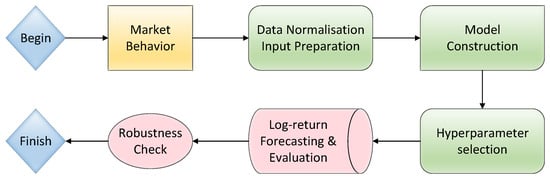
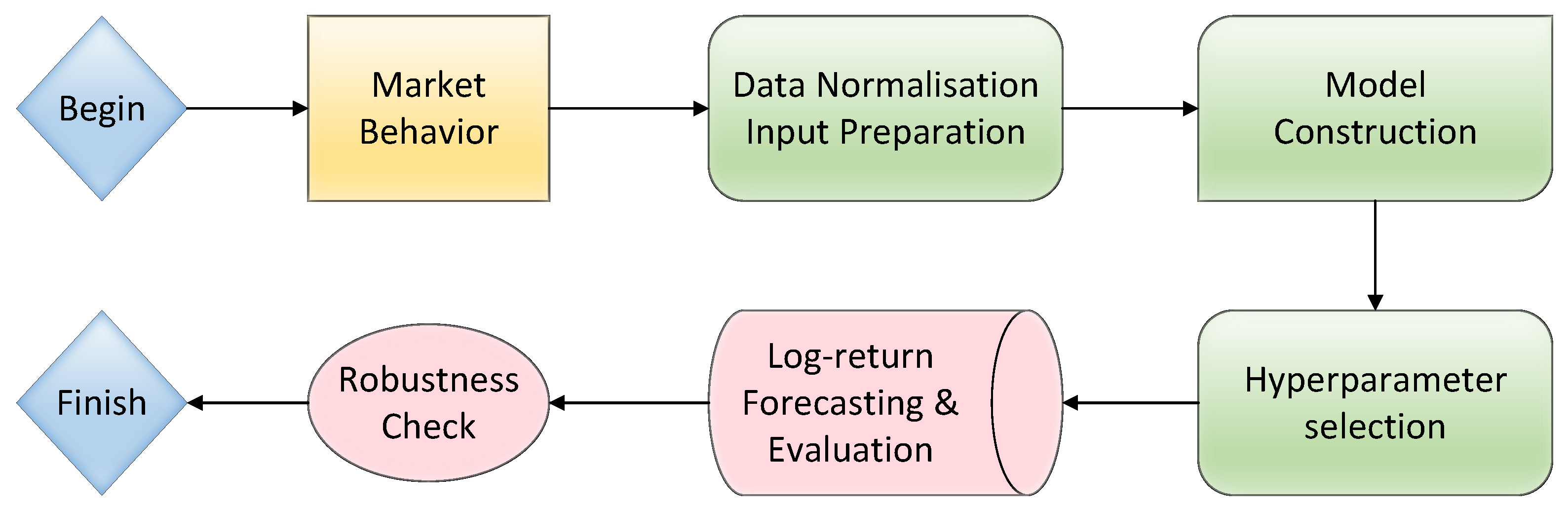
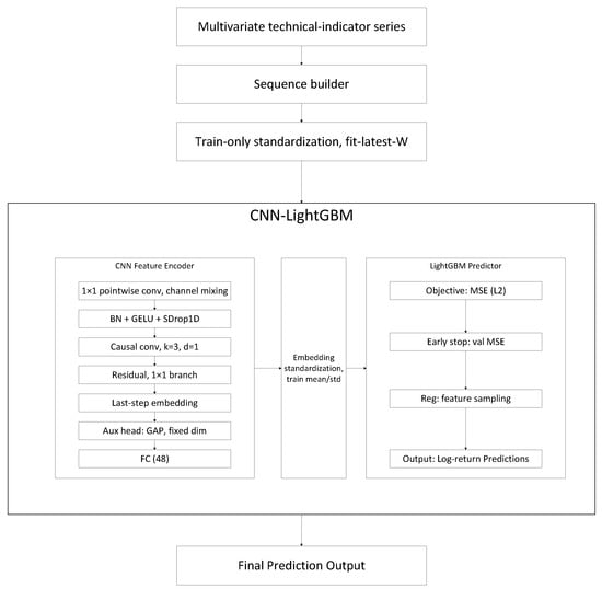
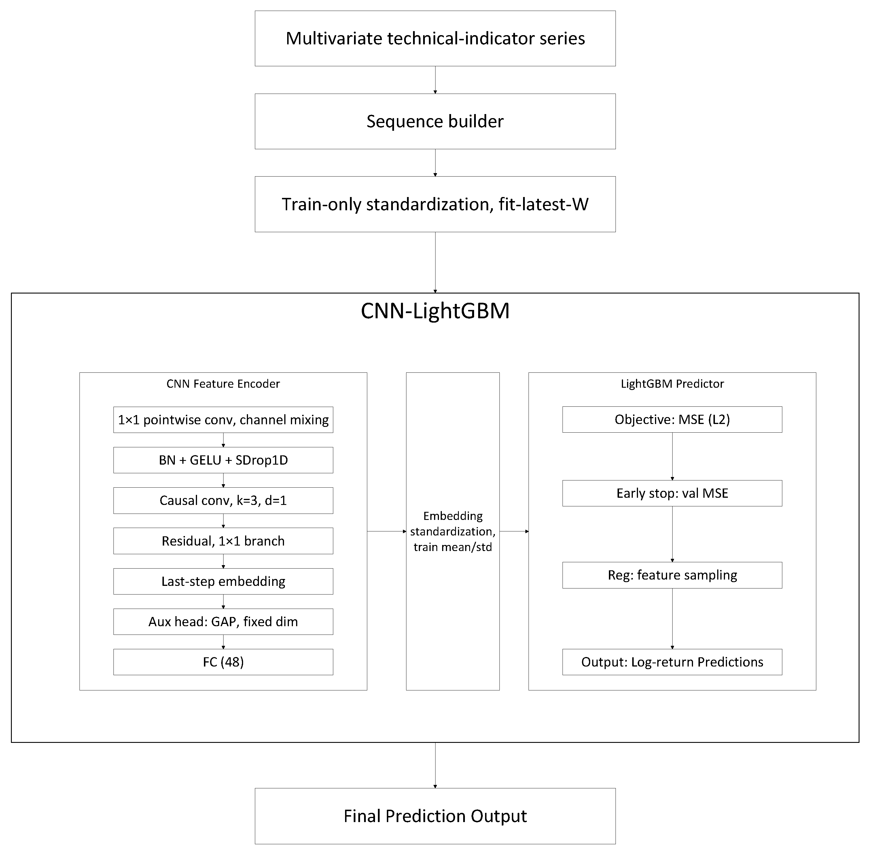
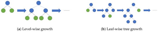
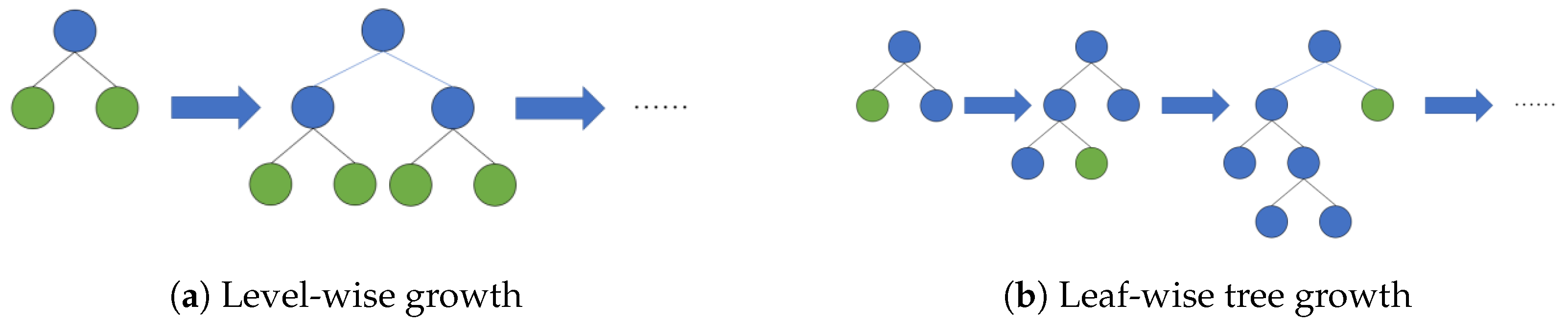
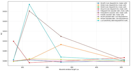
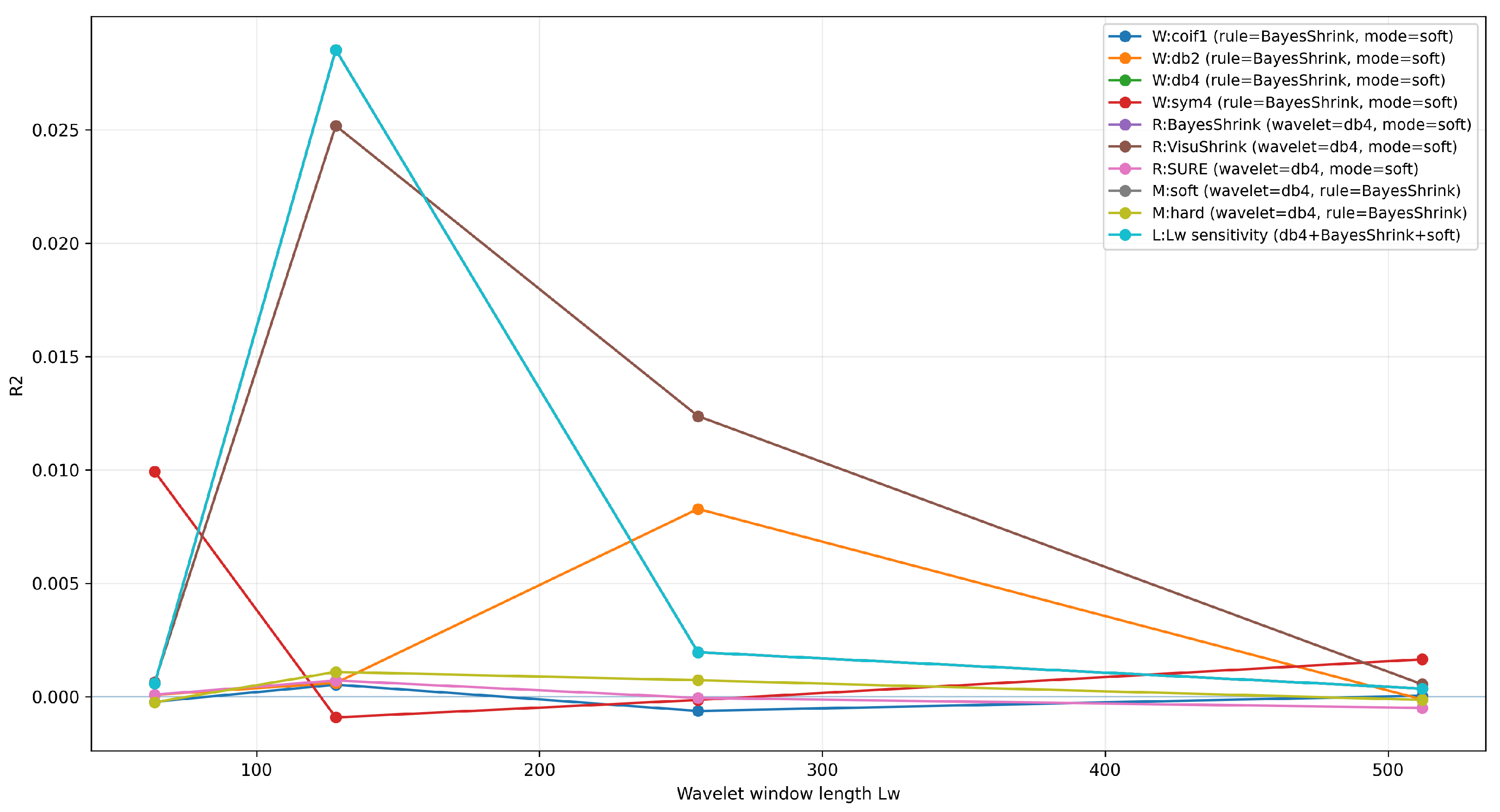
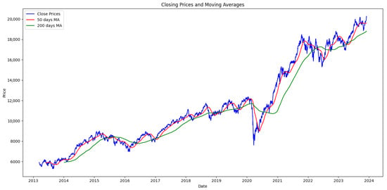
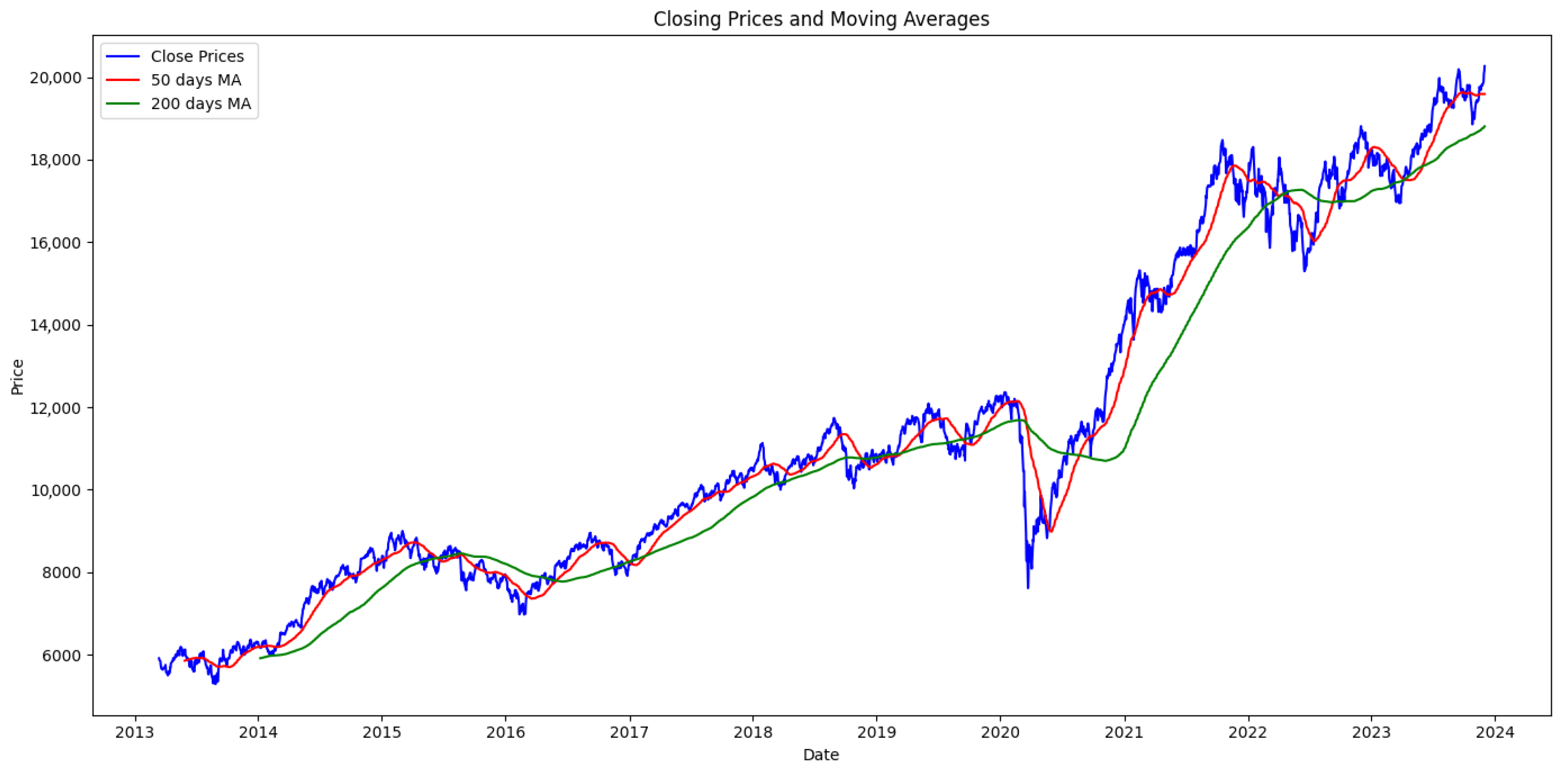
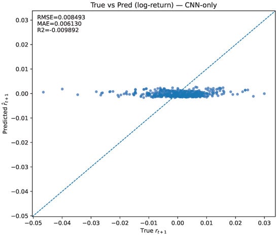
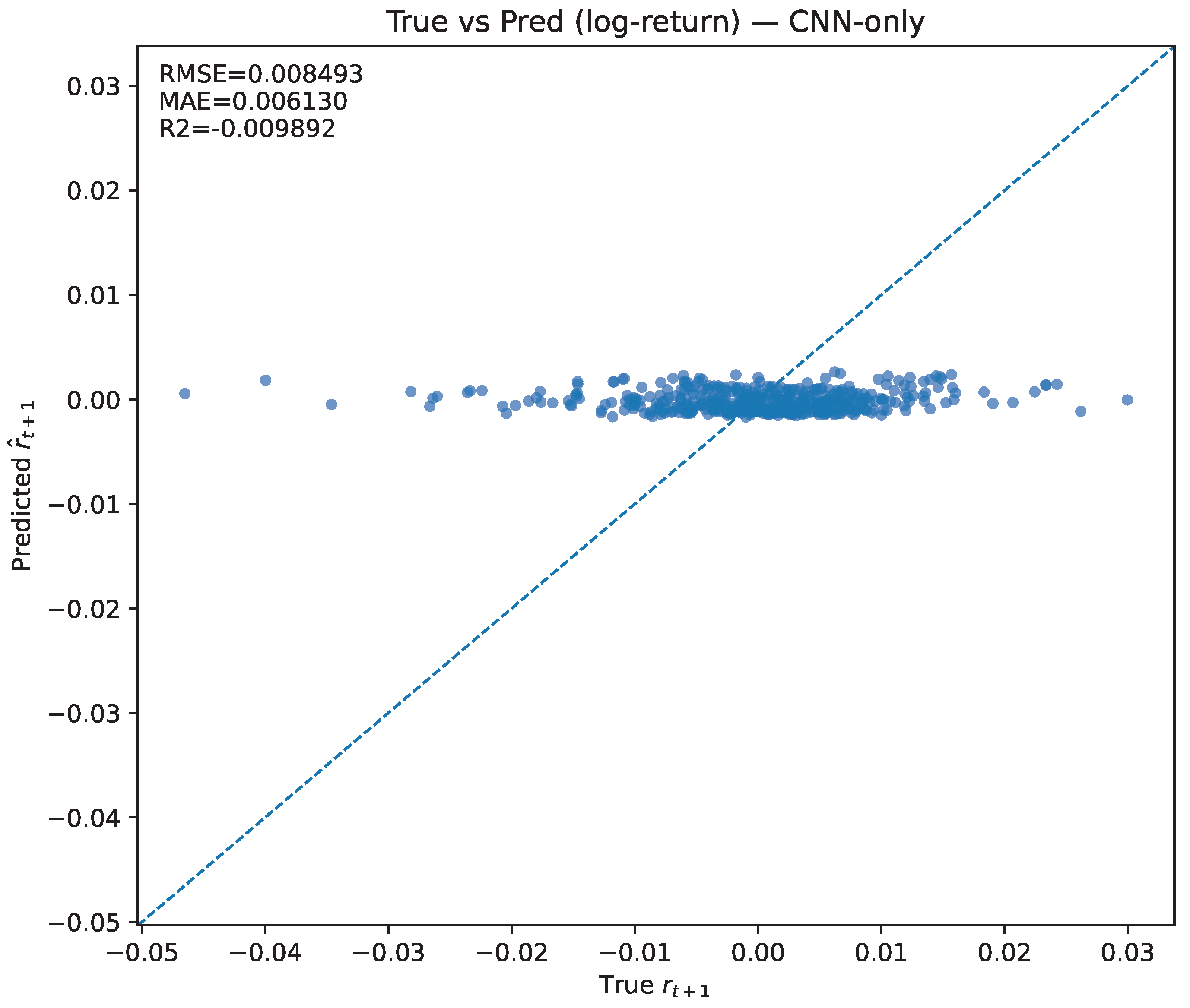
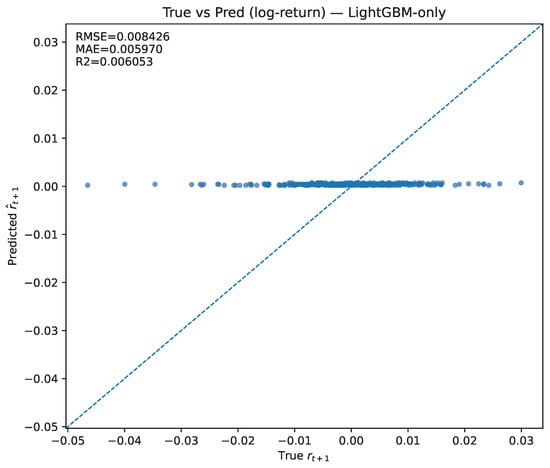
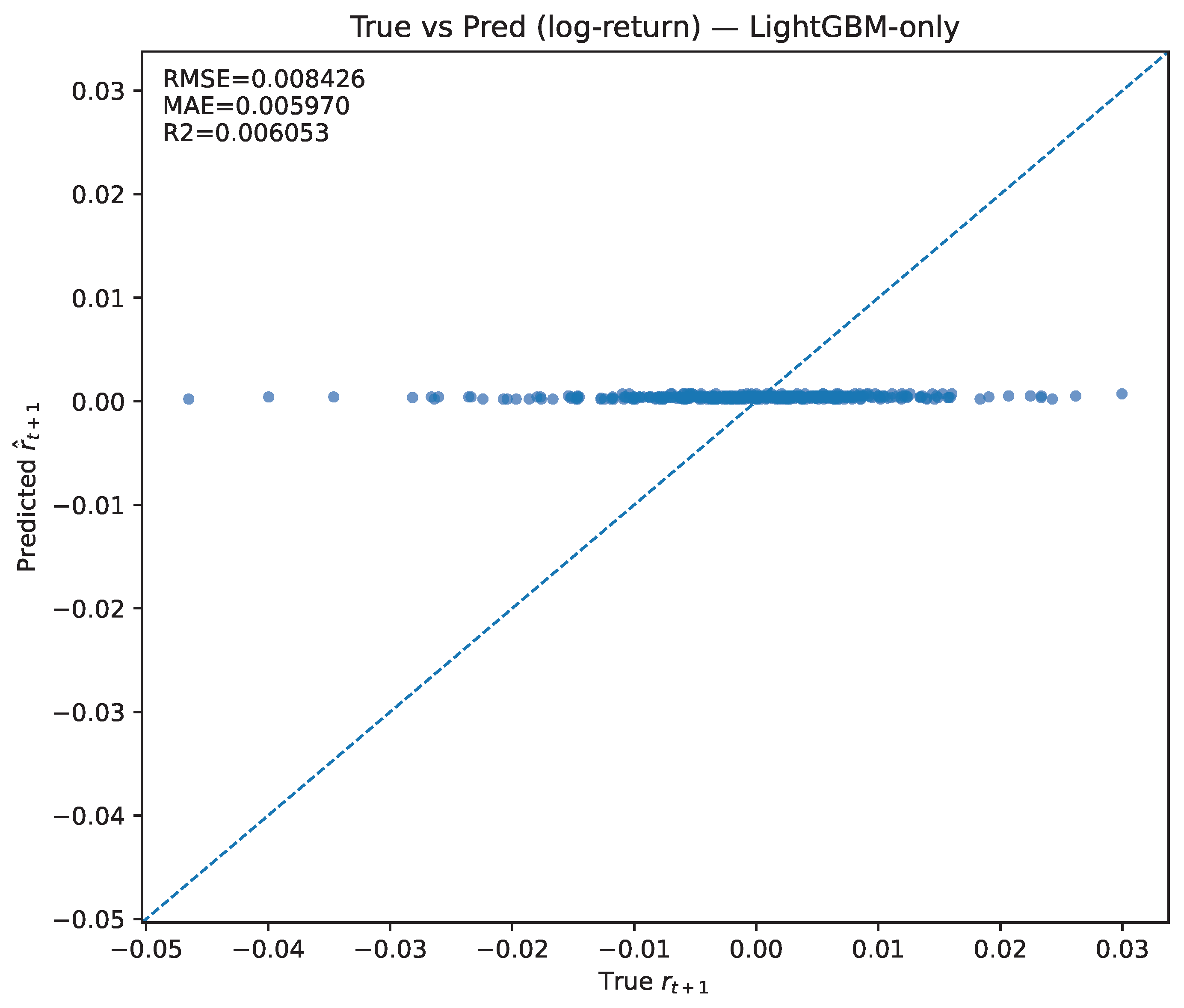
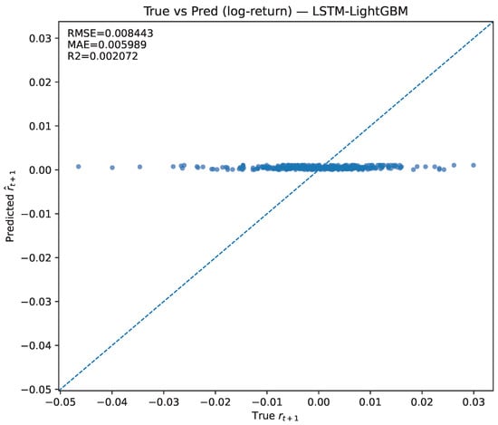
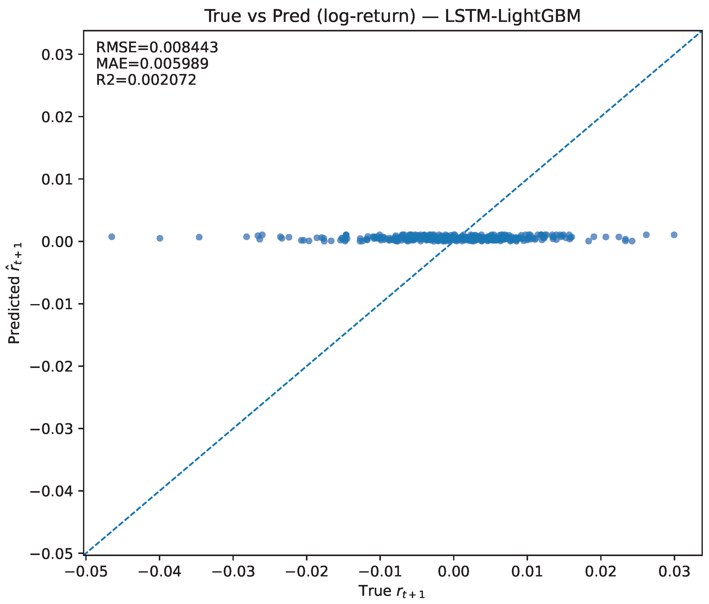
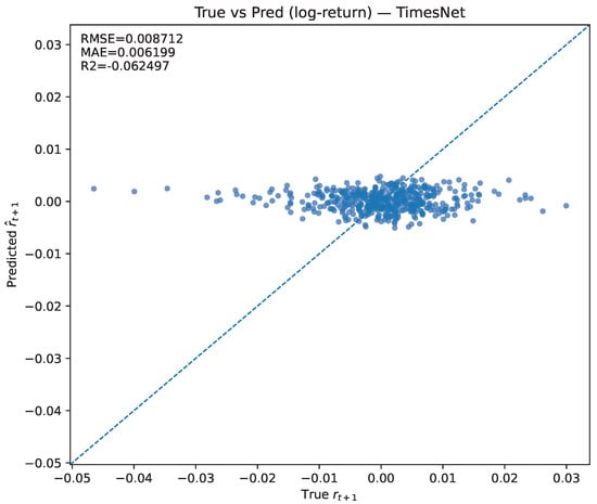
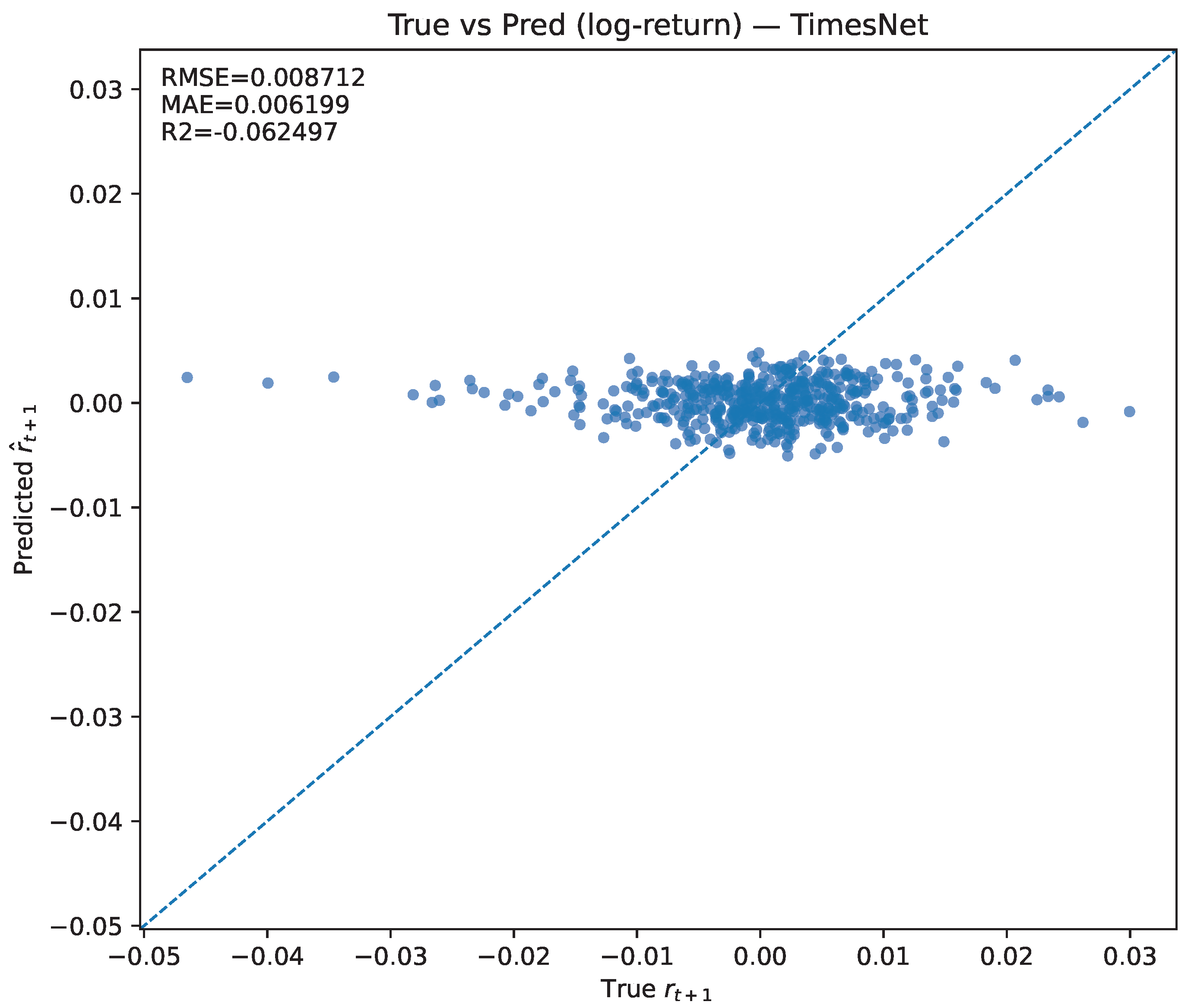
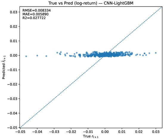
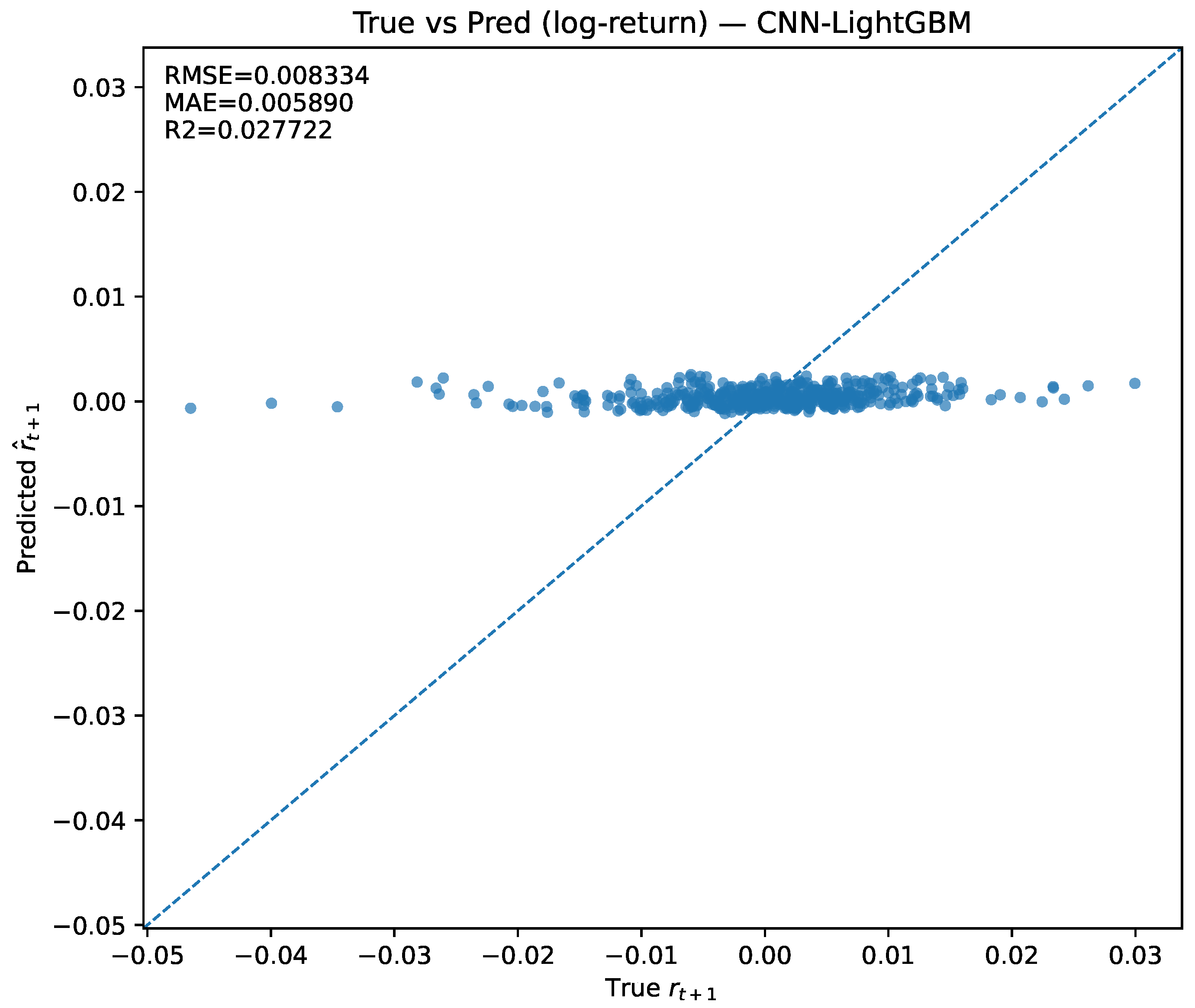
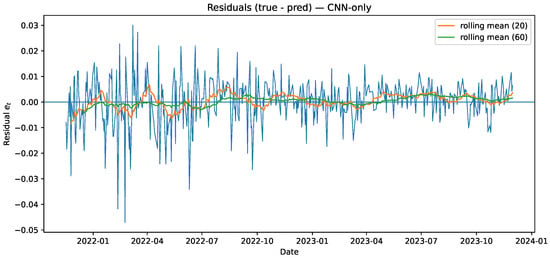
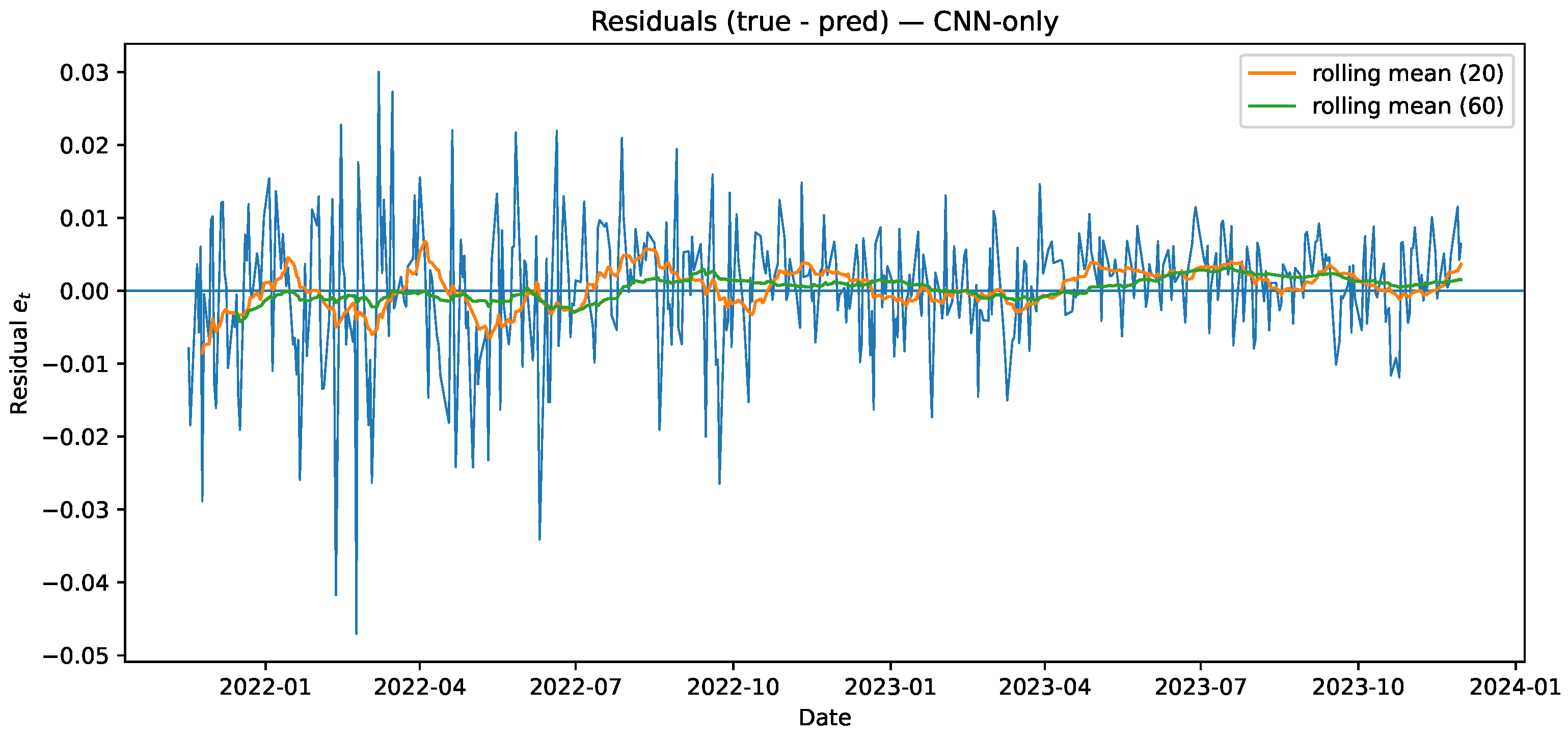
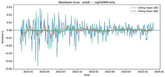
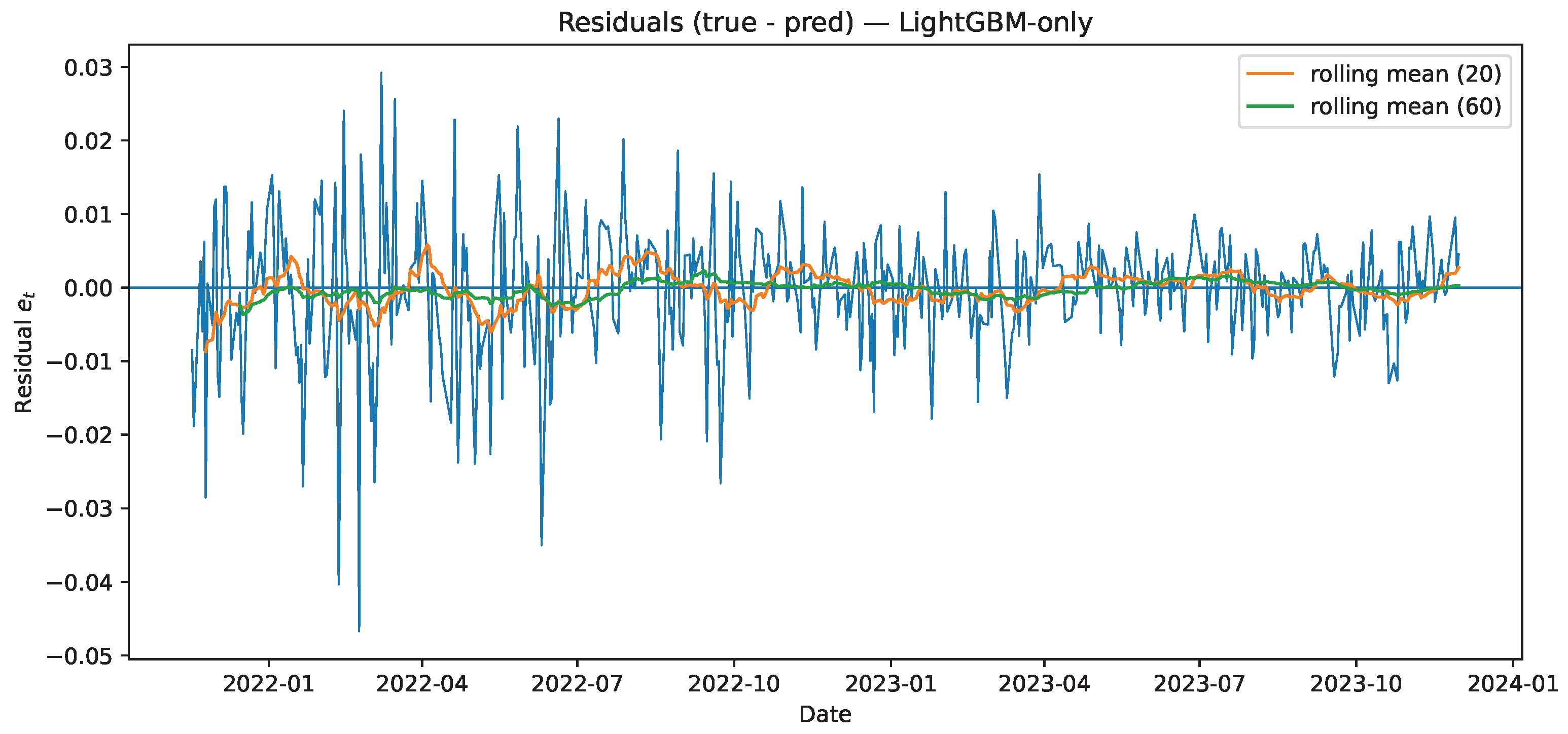
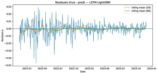
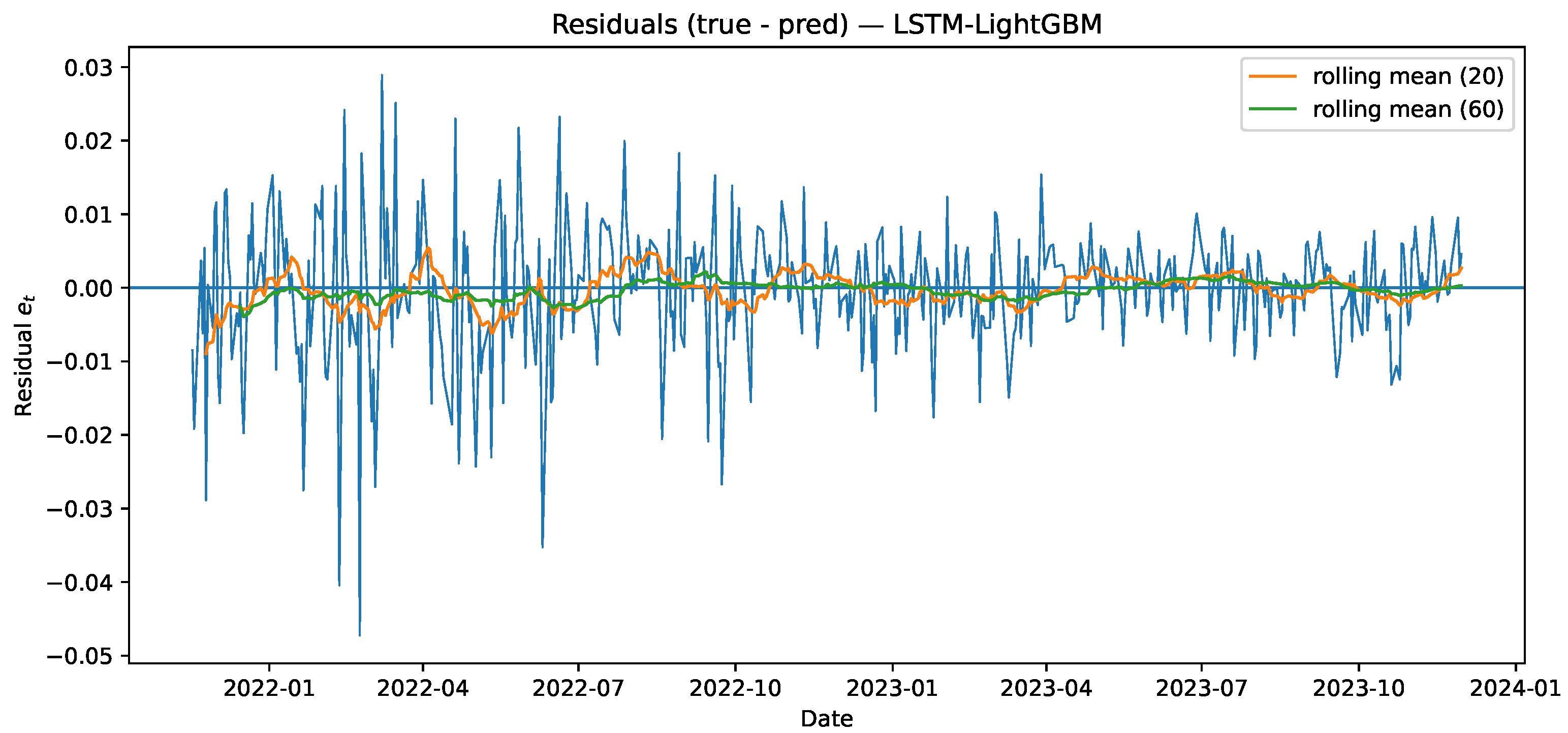
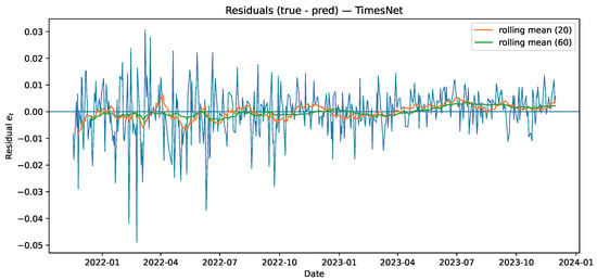
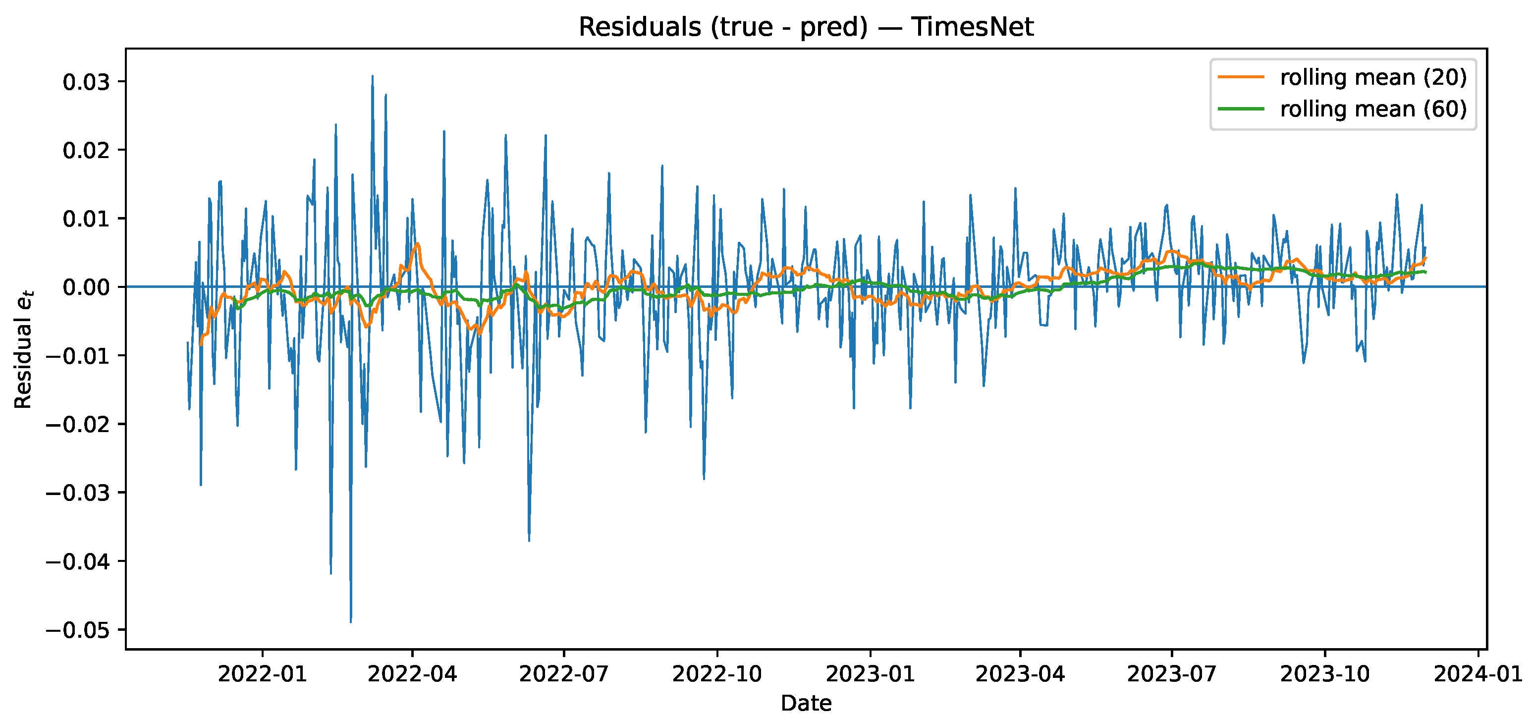
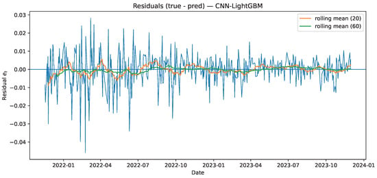
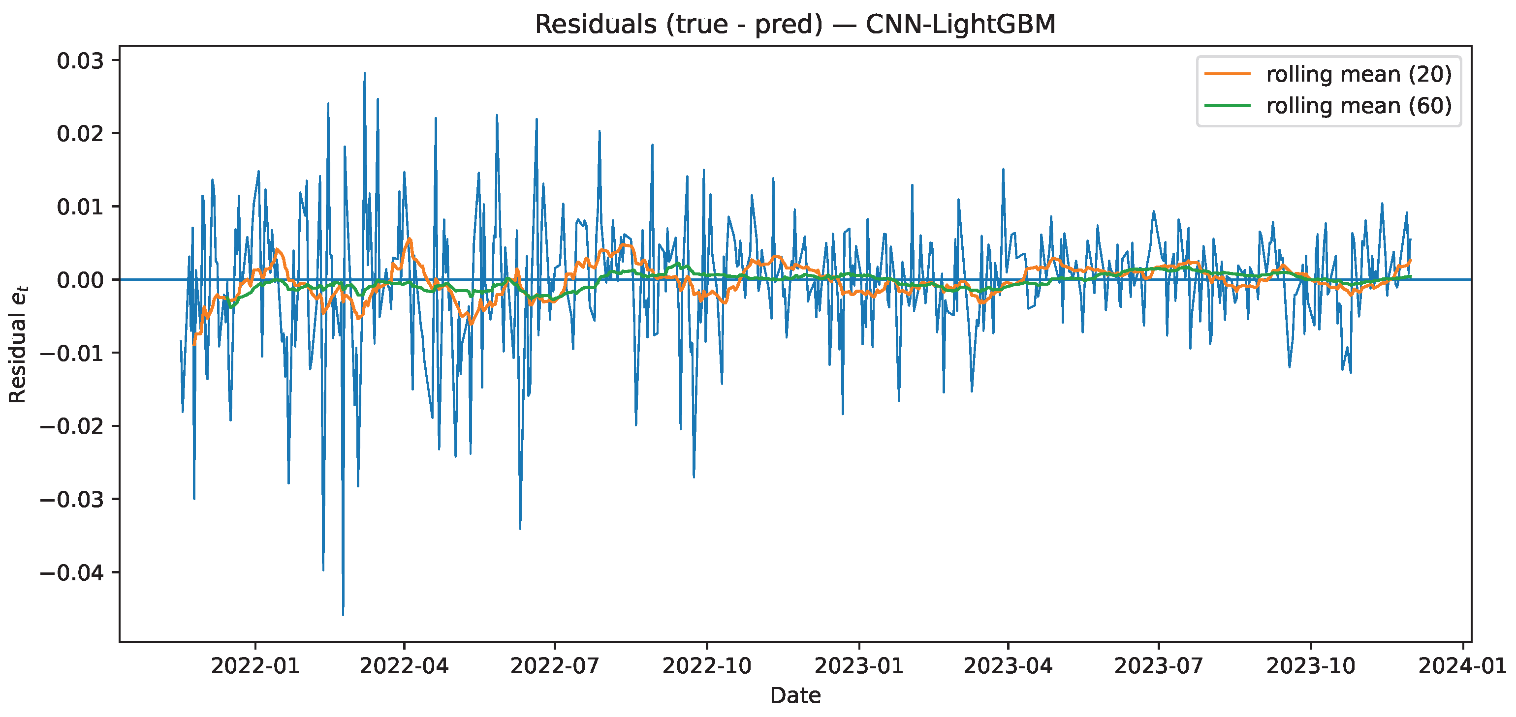
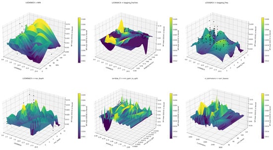
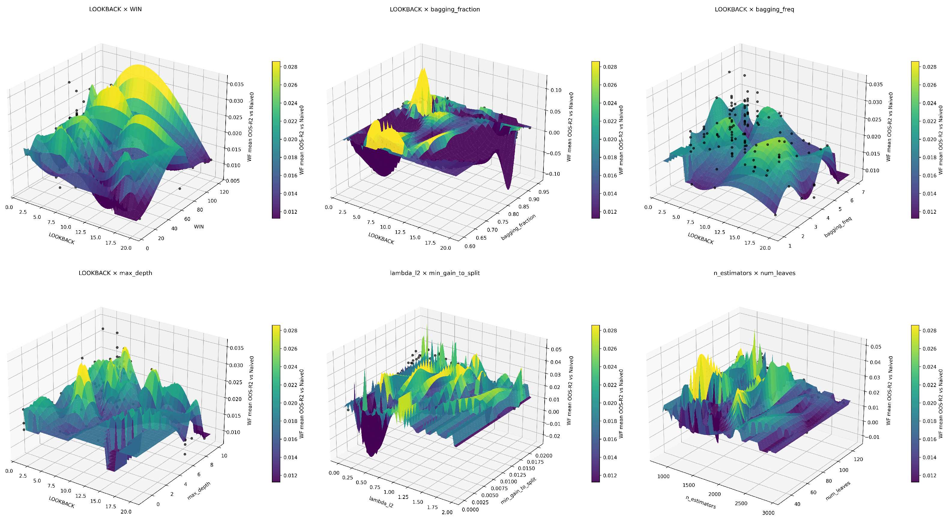
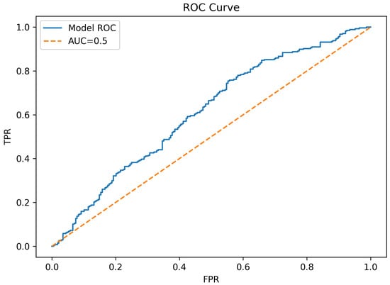
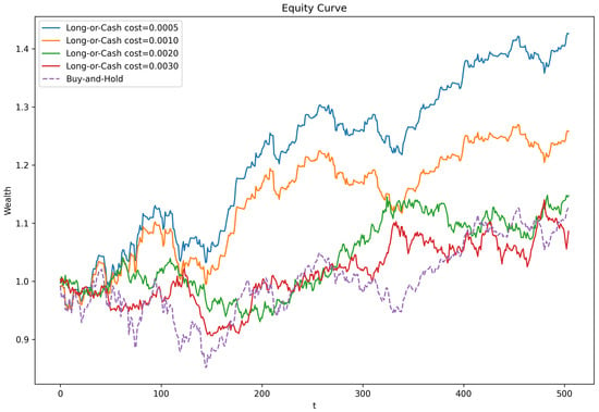
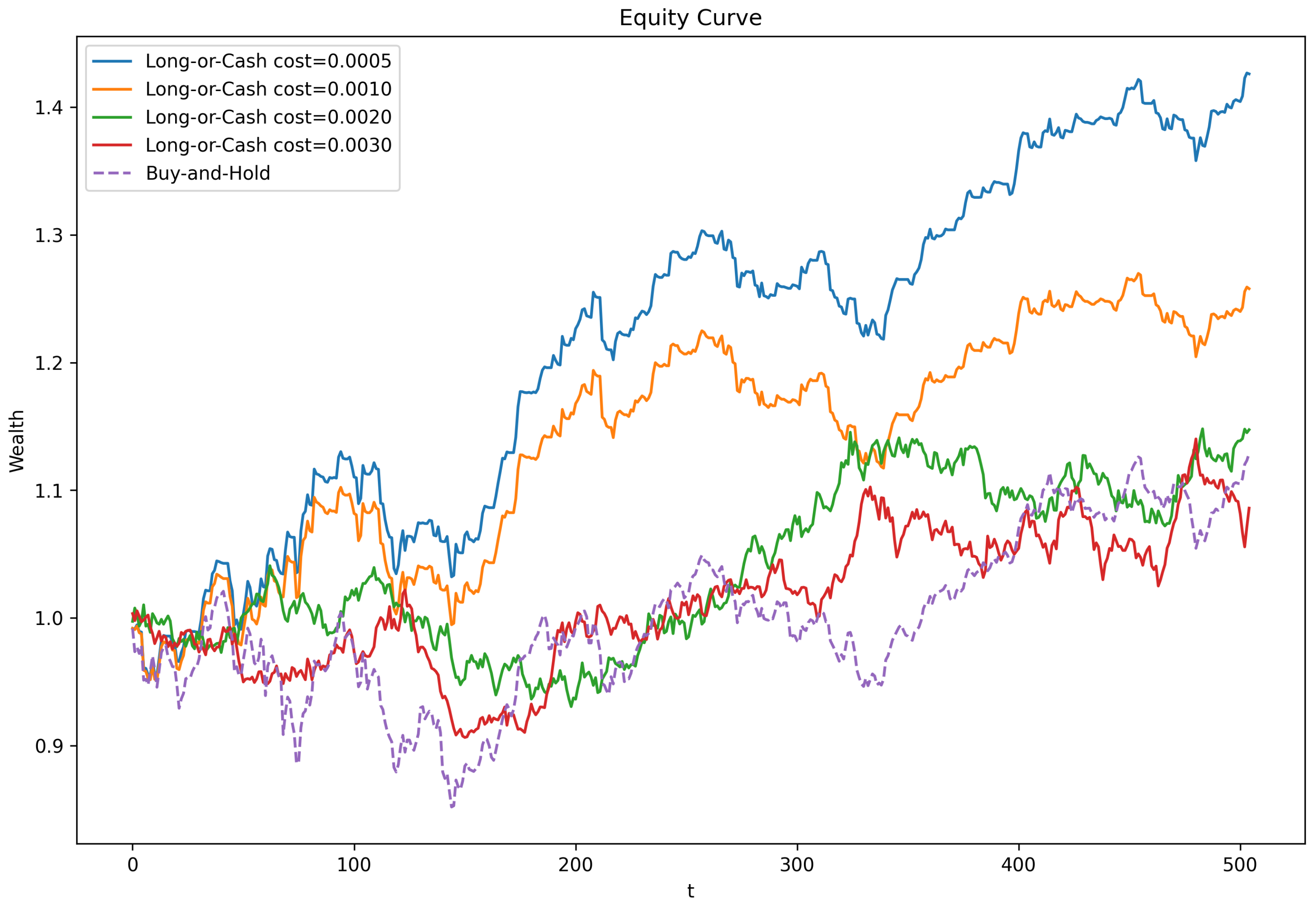

Disclaimer/Publisher’s Note: The statements, opinions and data contained in all publications are solely those of the individual author(s) and contributor(s) and not of MDPI and/or the editor(s). MDPI and/or the editor(s) disclaim responsibility for any injury to people or property resulting from any ideas, methods, instructions or products referred to in the content. |
© 2026 by the authors. Licensee MDPI, Basel, Switzerland. This article is an open access article distributed under the terms and conditions of the Creative Commons Attribution (CC BY) license.