


Abstract
This paper addresses single-machine due-window assignment scheduling with truncated learning effects and past-sequence-dependent setup times. In practical production systems, truncated learning effects capture the ceiling of skill improvement, past-sequence-dependent setup times reflect sequence-dependent switching efforts, and position-dependent weights allow varying importance across job positions. The due-window assignment includes the common, slack, and different assignments. The objective cost is the minimum of the weighted sum of earliness and tardiness, the number of early and tardy jobs, due-window cost, and the completion time. In which the weights are position-dependent. For the common and slack due-window assignments, several optimal structural properties are established. Based on these, the optimal schedule can be derived by solving a series of assignment problems, i.e., the problems can be solved in polynomial time , where n is the number of jobs. Under the common, slack, and different assignments without the number of early and tardy jobs cost, the optimal schedule of the problems can be obtained from an assignment problem, i.e., the problems can be solved in time. In addition, an extension of the job-dependent processing times is given. This study extends existing research models in this domain and proposes polynomial-time algorithms that guarantee optimal solutions for minimizing the objective cost function. The proposed approach not only advances scheduling theory by handling multiple realistic constraints simultaneously but also offers a practical decision-making tool for just-in-time production systems. The algorithms are tested numerically and compared with simulated annealing algorithm and tabu search algorithm.
MSC:
90B35
1. Introduction
In the modern production industry, scheduling models and problems can reduce production costs and improve efficiency (see Zhu and Wilhelm [1], Oron [2], Huang [3], Pei et al. [4], Zhao and Wang [5], Salama and Srinivas [6], Sun et al. [7], Ying et al. [8], Wu et al. [9], Wang et al. [10], Wang et al. [11], Liu and Shi [12], Liu et al. [13], Ge and Wang [14], Qiu and Wang [15], Li and Goossens [16], Miao et al. [17], Zhang et al. [18], Yuan et al. [19]). Scheduling problems with learning effects have been well studied (see Biskup [20], Li et al. [21], Yin [22], Azzouz et al. [23], and Jiang et al. [24]). Recently, Mor [25] considered a proportionate flow shop problem with learning effect and job rejection. For the makespan, total completion time, and total load minimizations, they proposed dynamic programming algorithms. Wang et al. [26] studied total completion time minimization in a single-machine problem. Under the position-weighted learning effect, they proposed a branch-and-bound algorithm. Sun et al. [27] addressed the flow shop scheduling with general learning effects. For total weighted completion time minimization, they proposed some heuristics and a branch-and-bound algorithm. Yin and Gao [28] and Yin et al. [29] considered the single-machine group technology scheduling with deteriorating setup times and learning processing times. Lv and Wang [30] studied flow shop scheduling jobs with learning and deterioration effects. Liu and Wang [31] addressed single-machine delivery times scheduling with learning effects. For the total weighted completion time (maximum tardiness) minimization, some heuristics and a branch-and-bound are proposed. Bai et al. [32] considered single-machine delivery times scheduling with variable processing times and rejection jobs. Under due-window assignment and two resource allocation functions, they showed that some problems are polynomially solvable. Zhang et al. [33] studied single-machine resource allocation scheduling with learning effects. In production scheduling or learning processes, as experience accumulates, the processing efficiency of jobs improves at a gradually slowing rate and eventually stabilizes, resulting in the truncated learning effects (). Lv and Wang [34] considered two-machine release dates for flow shop scheduling with truncated learning effects. For the total completion time minimization, they proposed some solution algorithms. Cohen and Shapira [35] conducted parallel identical machines scheduling with position-dependent processing times. For the makespan minimization, they presented an FPTAS (i.e., fully polynomial time approximation scheme) and some algorithms. The introduced scheduling research is all related to learning effects, whether it is position-dependent or time-dependent. Huang et al. [36] studied group scheduling with learning effects and resource allocations.
In 2008, Koulamas and Kyparisis [37] introduced the concept of past-sequence-dependent setup times (denoted by ). An example of the can be found in high-tech manufacturing, in which a batch of jobs consists of a group of electronic components mounted together on an integrated circuit board (see Koulamas and Kyparisis [37]). Then, some of the published papers considered different models of these problems: Cheng et al. [38], Hsu et al. [39], Wang and Liu [40], Lee [41], Soroush [42], Allahverdi [43], Mir and Rezaeian [44], and Mir et al. [45]. Recently, Jiang et al. [46] explored scheduling with the . Under learning effects, they proved that three problems are polynomially solvable. Zhao [47] studied single-machine scheduling with the truncated learning effects and . They proved that some regular objective costs are polynomially solvable. Wang et al. [48] conducted single-machine job rejection scheduling with deteriorating effects and . For the sum of scheduling cost (including makespan, total completion time, total absolute differences in completion (waiting) times), and total rejection cost minimization, they showed that the problem is polynomially solvable. Wang et al. [49] considered due-date assignment scheduling with the . For the non-regular objective cost of three due-date assignments (i.e., common due-date assignment (), slack due-date assignment (), and different due-date assignment (), see Geng et al. [50] and Shabtay et al. [51]); they showed that the problem is polynomially solvable. Wang [52] studied single-machine due-date assignment problems with the . Under the , , and , they proved that general earliness-tardiness cost minimization is polynomially solvable. Sun et al. [53] considered single-machine scheduling with the and linear deterioration. For the makespan and total completion time minimization, they proposed some solution algorithms. Truncated learning effect, as a type of learning effect, can better reflect the learning ceiling. In this processing environment, whether it affects the specified processing time and whether the job processing sequence changes accordingly are issues worth further study in scheduling problems.
In the just-in-time (JIT) scheduling (e.g., the due-window problems, see Janiak et al. [54], Lu et al. [55], Yue and Zhou [56], Lv and Wang [57], Zhang and Yin [58], and Song et al. [59]), most of the papers consider the objective of minimizing the sum of earliness and tardiness. For a general objective, i.e., the weighted sum of the number of early/tardy jobs and earliness/tardiness duration, Liu et al. [60] considered the single-machine due-window assignment scheduling with the . Under three due-window assignments (i.e., common due-window assignment (, Tian [61], Ren and Yang [62]), slack due-window assignment (, Tian [61], Liu [63], Zhang et al. [64]) and different due-windows assignment (, Liu [63])), they proved that the general earliness-tardiness cost minimization is polynomially solvable. In this paper, we continue the work of Liu et al. [60], but study the due-window assignment scheduling with and positional-dependent weight, which indicate the importance of the corresponding positions (see Wang et al. [65], Wang et al. [66]), which combines the work of Liu et al. [60] and Wang et al. [65]. In addition, a model with job-dependent processing times is also considered, enabling a more comprehensive analysis of the problem by simultaneously considering both position- and time-dependent processing time functions. Under optimal properties of the common, slack, and different assignments, we prove that the problems are polynomially solvable.
This study integrates truncated learning effects (controlled by parameter ) with past-sequence-dependent setup times (modulated by parameter ) to construct a scheduling model that better reflects real-world complexities. The model accurately captures key features of scheduling scenarios, such as the existence of an upper limit to productivity improvement and the dependence of task-switching costs on historical sequences. It finds wide application in fields such as electronic assembly, printing and spraying, chemical production, and medical scheduling. Addressing issues caused by traditional models that overlook these practical dependencies—such as overly optimistic planning, resource idling, and efficiency losses—the comprehensive model and polynomial-time optimal algorithms proposed in this paper enable the synergistic optimization of learning gains and task sequencing. This allows for the overall minimization of comprehensive metrics, including total weighted completion time, earliness/tardiness penalties, and due-window costs, under multiple constraints. This work not only extends scheduling theory but also provides an efficient decision-making tool with guaranteed optimality for modern manufacturing and service systems implementing lean production and JIT practices, demonstrating significant theoretical value and practical relevance. In addition, this study introduces position-dependent weights to characterize the importance differences among various processing positions. For example, in single-machine scheduling or flow-shop scheduling, as the processing sequence advances, equipment may experience cumulative thermal wear, tool deterioration, or precision decline due to continuous operation. Jobs processed at later stages face higher risks or costs in terms of processing quality or required time due to degraded equipment conditions, thus necessitating higher weights to reflect such risk premiums. For products whose value increases progressively with processing stages, such as semiconductor wafers, jobs at later processing stages possess higher value and incur greater work-in-progress inventory costs. Higher position-dependent weights can capture the varying impacts caused by early or tardy completion of such high-value in-process items.
This paper addresses a single-machine due-window assignment scheduling problem that incorporates past-sequence-dependent setup times, truncated learning effects, and position-dependent weights. Compared to existing works in the literature (i.e., Liu et al. [60] and Wang et al. [65]), the core contribution of this research lies in the integration of these three key factors and the successful proof that the problem remains solvable via polynomial-time optimal algorithms under three types of due-window assignment. This not only extends the capability of scheduling theory to model complex real-world factors but also provides decision-makers with effective solution approaches. The remaining part of the paper is organized as follows. Section 2 contains the formulation. Section 3 shows that the models , , and are polynomially solvable. Section 3 also presents an extension. Section 4 gives an example and the numerical tests. Section 5 presents the results and discussion. Section 6 concludes the paper.
2. Problem Formulation
Assume that n jobs are to be processed on a single-machine. If job is placed in the rth position, its actual processing time can be written according to truncated learning effects (TLE) as follows:
where is the normal processing time of , denotes the learning curve of scheduled in the rth position (e.g., , denotes the learning factor; , ; , ; and so on), and is the truncated parameter. Let be some job scheduled in the th position, the (past-sequence-dependent setup times) of is:
where is the actual processing time of , and is the setup time rate. The total processing time requirement of is
Let (resp. ) represent the completion time (resp. due-window) of , where (resp. ) is the starting (resp. finishing) time of the due-window, and is the due-window size of (see Janiak et al. [54], Tian [61], Sun et al. [67], Wang et al. [68]). For the model, , and is the size of the , and are decision variables. For the model, , and is the size of the , and are decision variables. For the model, each job has its own due-window, i.e., and () are decision variables. Let (resp. ) be the earliness (resp. tardiness) of , (resp. ) be the number of early (resp. tardy) jobs . Our goal is to minimize the general earliness–tardiness cost:
where () is the positional-dependent weight and non-negative, which does not change with the variation of the job (see Qian et al. [69], Qian and Guo [70], Wang et al. [71]). As in Graham et al. [72], Pinedo [73], and Gawiejnowicz [74], the problem can be denoted by
where .
Let be the due-date of , for the , ( is a decision variable); for the , ( is a decision variable), for the , each is a decision variable. Under the due-date assignments, we have: the earliness (resp. tardiness) of is (resp. ), the number of early (resp. tardy) job is (resp. ).
The relevant symbols and their meanings discussed in this article are presented in Table 1.
Table 1.
Symbol explanation and meaning.
The models with , position-dependent processing times and/or due-window (due-date) assignments studied are presented in Table 2.
Table 2.
Models with , position-dependent processing times and/or due-window (due-date) assignments.
3. Proposed Algorithm
Obviously, for the models , , and , an optimal schedule exists such that all jobs are processed consecutively at time 0 and can not be interrupted.
3.1. Models and
To determine the optimal positions of the due-window, we first establish the following lemmas.
Lemma 1.
For a given schedule τ of , there exists an optimal solution such that: , where
and
.
Proof.
(1) Assume and , we have
However, when and , it follows that
When and , it follows that
From Equations (8)–(10),
and
If , then ; if , then . That is, is equal to some job’s completion time, i.e., . Similarly, is equal to some job’s completion time, i.e., .
(2) Let and , we have
Using a small perturbation analysis on the window starting time , compare the cost when is slightly shifted before or after a job completion time. This analysis yields the critical condition that must be satisfied by the optimal index x.
If ( and ) and , we have
If ( and ) and , we have
By the small perturbation method, from Equations (13)–(15), it follows that
and
Thus, from Equations (16) and (17), . Since it is impossible to find the value of , it can only find that .
Similarly, for the value y, we have . □
Lemma 2.
Proof.
Similar to Lemma 1. □
Lemma 3.
For a given schedule τ of , the completion time
Proof.
From Equations (2) and (3), by the mathematical induction, we have
where . □
For a given schedule of , from Lemmas 1 and 3, we have , and . Thus
and
Similarly, for the model , from Lemmas 2 and 3, we have , and . Thus
and
From Equations (1), (19) and (21), if , for models and , we have
If x and y are given, let
then the optimal schedule of is obtained by the assignment problem (denoted by ):
where
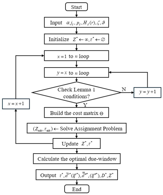
From the above analysis, to solve , the optimal algorithm can be clearly presented. The core idea of this algorithm is to enumerate all feasible due-window position pairs that satisfy the structural conditions given in Lemma 1; for each candidate pair, an assignment problem is solved to obtain the optimal job sequence and its corresponding cost under that condition; finally, the scheduling solution with the lowest total cost among all candidates is selected as the globally optimal solution. The detailed steps of Algorithm 1 are as follows, and the flowchart is shown in Figure 1.
Figure 1.
The flowchart of Algorithm 1.
| Algorithm 1 |
| Input: (), , , , |
| Output: An optimal schedule , , (such ), |
| 1. initialize |
| 2. for to n do |
| 3. for to n do |
| 4. // Check the conditions for from Lemma 1 |
| 5. if and |
| 6. // Build the cost matrix for the Assignment Problem |
| 7. then initialize cost matrix |
| 8. for each job to n do |
| 9. for each position to n do |
| 10. |
| 11. // is from Equation (20) for or Equation (22) for |
| 12. if |
| 13. then |
| 14. else if |
| 15. then |
| 16. end if |
| 17. end for |
| 18. end for |
| 19. // Solve the Assignment Problem with cost matrix |
| 20. |
| 21. |
| 22. // Add the constant terms to the objective value |
| 23. if |
| 24. then |
| 25. |
| 26. , |
| 27. end if |
| 28. end if |
| 29. end for |
| 30. end for |
| 31. // Calculate the optimal due-window times based on the best schedule |
| 32. if model |
| 33. then , |
| 34. |
| 35. else if model |
| 36. then , |
| 37. |
| 38. end if |
| return , , , |
| end |
Now, analyze the time complexity of Algorithm 1. Theorem 1 is presented as follows:
Theorem 1.
is solved in time by Algorithm 1.
Proof.
Since and , , there are at most possibilities for , so the required time is . It needs time to calculate . It takes time by Hungarian Algorithm to solve the for each . Thus, is solved by Algorithm 1 in time. □
If , i.e.,
Similarly, we have:
Lemma 4.
For a given schedule τ of
there exists an optimal solution such that: , where
and
.
Lemma 5.
For a given schedule τ of
there exists an optimal solution such that: , where x is determined by Equation (29), and y is determined by Equation (30), .
From Lemmas 4 and 5, for the models and , the optimal schedule of
is obtained by the (25)–(26), where
for the , is given by Equation (20); for the , is given by Equation (22), .
Based on the above analysis, the optimal method for solving
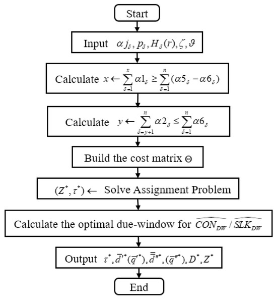
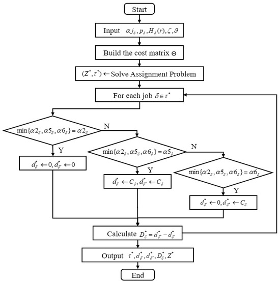
can be clearly described. When the penalty costs for the number of early and tardy jobs are excluded from the objective function (i.e., ), the problem is further simplified. In this case, the optimal positions of the due-window, x and y, can be directly determined via Lemma 4 without enumerating all possible combinations. The algorithm obtains the globally optimal schedule by solving an assignment problem, and the time complexity is correspondingly reduced. The specific steps of Algorithm 2 are as follows, and the flowchart is shown in Figure 2.
Figure 2.
The flowchart of Algorithm 2.
| Algorithm 2 of |
| Input: (), , , , |
| Output: An optimal schedule , , (such ), |
| 1. // Step 1: Determine optimal due-window positions |
| 2. Find the smallest integer such that: |
| 3. Find the smallest integer such that: |
| 4. // Step 2: Build and solve the assignment problem |
| 5. initialize cost matrix |
| 6. for each job to n do |
| 7. for each position to n do |
| 8. if model |
| 9. then using Equation (20) |
| 10. else if model |
| 11. then using Equation (22) |
| 12. end if |
| 13. |
| 14. end for |
| 15. end for |
| 16. // Solve the Assignment Problem with cost matrix |
| 17. |
| 18. // Step 3: Calculate the optimal due-window times based on the optimal schedule |
| 19. if model |
| 20. then , |
| 21. |
| 22. else if model |
| 23. then , |
| 24. |
| 25. end if |
| return , , , |
| end |
Theorem 2.
is solved in time by Algorithm 2.
Proof.
Step 1 needs time by the , Step 2 needs time, Step 3 needs time, thus, is solved by Algorithm 2 in time. □
3.2. Model
In this subsection, we assume that , i.e.,
For a given schedule of , the objective cost of is
Lemma 6.
For a given schedule τ of , there is an optimal property such that .
Proof.
Similar to Liu et al. [60]. □
Lemma 7.
For a given schedule τ of , the optimal due-windows are:
- (i). If , we have ();(ii). If , we have ();(iii). If , we have ().
Proof.
For a given schedule of model from Lemma 6 and Equation (33), , and the function for is
Obviously, if , then , and should be 0, i.e., . If , should be and . If , then should be 0 and should be . □
From Lemma 7, for case (i), we have ; for case (ii), we have ; for case (iii), we have , hence, we have
From Koulamas and Kyparisis [37], , hence
Then the optimal schedule of is obtained by the (25)–(26), where
Based on the above analysis, the following algorithm is proposed to solve
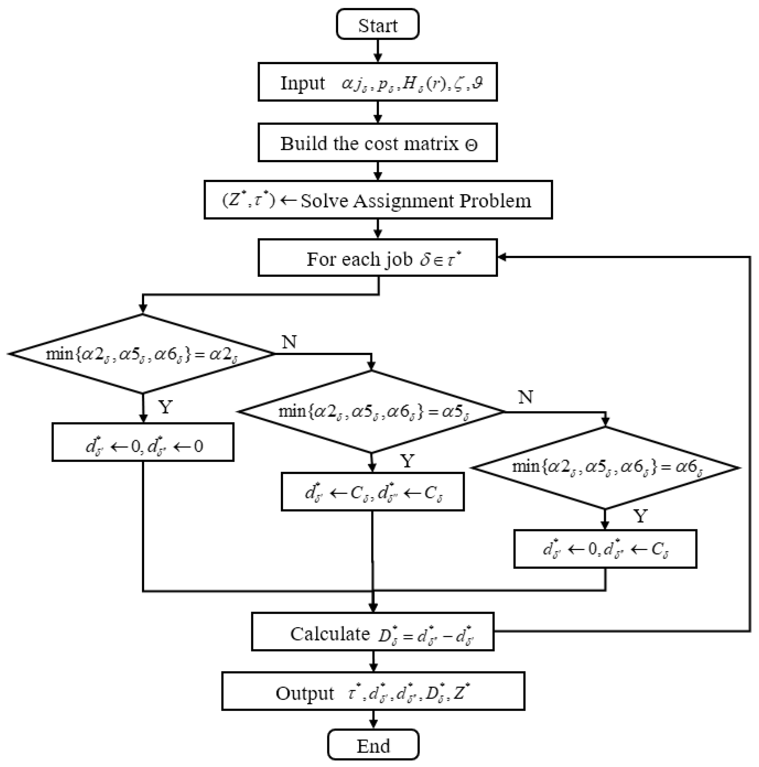
Under the condition where the penalty costs for early and tardy jobs are omitted from the objective function (i.e., ), the problem exhibits a more concise structural property. According to Lemma 7, the optimal due-window for each job can be directly determined based on its processing time and weight parameters, while the overall optimal schedule can still be obtained by solving an assignment problem. The steps of Algorithm 3 are as follows, and the flowchart is shown in Figure 3.
Figure 3.
The flowchart of Algorithm 3.
| Algorithm 3 of |
| Input: (), , , , |
| Output: An optimal schedule , , (such ), |
| 1. // Step 1: Build and solve the Assignment Problem for optimal schedule |
| 2. initialize cost matrix |
| 3. for each job to n do |
| 4. for each position to n do |
| 5. // Calculate position-dependent coefficient for model |
| 6. |
| 7. |
| 8. end for |
| 9. end for |
| 10. // Solve the Assignment Problem with cost matrix |
| 11. |
| 12. // Step 2: Calculate optimal due-window times for each job in the optimal schedule |
| 13. Calculate completion times for all positions to n in schedule |
| 14. For each job in schedule do |
| 15. if |
| 16. then , |
| 17. else if |
| 18. then , |
| 19. else if |
| 20. then , |
| 21. end if |
| 22. |
| 23. end for |
| return , , , |
| end |
Theorem 3.
is solved in time by Algorithm 3.
Proof.
Similar to Theorem 2. □
3.3. An Extension
In this subsection, we introduce job-dependent processing times (see Liu [75]; Zhu et al. [76]; Zhang et al. [77]; Sanchez-Herrera et al. [78]; Przybylski [79]; and Gerstl and Mosheiov [80]) to the model, i.e., the actual processing time of is: , where is the actual processing time of is scheduled in rth position (e.g.,
denotes processing time when is scheduled in rth position, , is the aging factor (see Mosheiov [81]), , is the aging factor of , , is (see Gordon [82]), , , and so on). For example, (see Example 1 in Mor [83]),
From Section 3.1, for the models and , we have
where, for the , is given by Equation (20); for the , is given by Equation (22), .
Similar to Section 3.1, for the models and , if x and y are given, the optimal schedule of is obtained by the (25)–(26), where
in which, for the , is given by Equation (20); for the , is given by Equation (22), .
Theorem 4.
is solved in time.
Similar to Section 3.1 and Section 3.2, if , for models , and , the optimal schedule of
is obtained by the (25)–(26), where
in which, for the , is given by Equation (20); for the , is given by Equation (22); for the , .
Theorem 5.
is solved in time.
4. Computational Experiments
4.1. An Example
Focus on , where , , , , , , , ; the positional-dependent weights are given in Table 3.
Table 3.
Values of .
For the model , from Equation (6) in Lemma 1, i.e., , we have ; from Equation (7) in Lemma 1, i.e., , we have .
For and , ; the sub-optimal schedule is , the values (from Equation (20)) are , , , , ; and are presented in Table 4 (see Equation (27)).
Table 4.
Values for and (bold numbers are the sub-optimal solution).
Table 5.
Results of all pairs of x and y.
From Table 5, the optimal solution is: and , ; the optimal schedule is , and .
4.2. Numerical Simulation
To validate the performance of Algorithms 1–3 presented in this paper, we conducted numerical simulation experiments in this section. Additionally, in scheduling research, simulated annealing (denoted as ) and tabu search (denoted as ) are widely recognized as well-established and efficient optimization algorithms (see Sun et al. [84] and Li et al. [85]). Therefore, they are included in this study for comparison with the algorithm proposed in this paper. In this experiment, the relevant parameters for the algorithm were set as follows: (1) tabu list size: 20 and (2) candidate list size: 10. The parameters for the algorithm were set as: (1) initial temperature: 1000; (2) cooling rate: 0.95; and (3) final temperature: . The maximum number of iterations for both algorithms was set to 1000n. For comparison, we introduced the Simulated Annealing algorithm (denoted as , see Sun et al. [84]) and the Tabu Search algorithm (denoted as , see Li et al. [85]). We coded these algorithms in PyCharm Community Edition 2024.1.3 and ran the computational experiments on a PC with a CPU 12th Gen Intel(R) Core(TM) i5-12400 2.50 GHz, 16.00 GB RAM, and a Windows 11 operating system. All instances in the experiments were generated based on the random number generation method provided by Taillard [86], with the initial random seed set to 20. The parameter ranges used in this experiment are as follows:
(1) ;
(2) were uniformly sampled from [1, 100];
(3) and ;
(4) () were uniformly sampled from [0.1, 1], [1, 10], or [10, 100];
(5) was used, and .
For each parameter combination, 30 random runs were conducted. Experimental results recorded the CPU time (in seconds) required for each algorithm’s execution, along with the error rates of and . The error rate was calculated using formula , where H denotes the solution obtained by or , while represents the optimal solution obtained by Algorithms 1–3. Table 6 and Table 7 and Table 8 and Table 9, respectively, document the comparison results between Algorithms 1 and 2 under and conditions versus and (Note: Algorithm 2 was used to solve problems under conditions.); Table 10 records the performance comparison results of Algorithm 3 with and under condition.
Table 6.
Results of Algorithm 1 with and ().
Table 7.
Results of Algorithm 1 with and ().
Table 8.
Results of Algorithm 2 with and ( and ).
Table 9.
Results of Algorithm 2 with and ( and ).
Table 10.
Results of Algorithm 3 with and ().
5. Results and Discussion
Based on the experimental results, under different weights of the same scale, the running time and error rates of each algorithm show no significant variation. This indicates minimal influence of weights on algorithmic performance. Further analysis of the experimental results reveals that in terms of computational efficiency, the maximum CPU times for Algorithms 1–3 are only 102.07 s, 0.08 s, and 0.01 s, respectively, significantly lower than those of the and algorithms, demonstrating a clear time efficiency advantage. Regarding solution quality, and struggle to guarantee optimal solutions for this problem, with maximum error rates of 1.069 and 1.052, respectively. In contrast, Algorithms 1–3 proposed herein can obtain optimal solutions. In summary, whether in computational efficiency or solution accuracy, Algorithms 1–3 proposed in this paper significantly outperform traditional and algorithms, validating their effectiveness and superiority.
Although is a polynomial-time algorithm in theory, its computational cost grows relatively rapidly with problem size. In practical scheduling, the number of jobs n is usually within an acceptable range (e.g., ), and the algorithm proposed in this paper remains feasible. Our numerical experiments show that for , the algorithm’s running time is still within an acceptable limit (approximately 102 s in the worst case) and significantly outperforms heuristic algorithms such as Simulated Annealing and Tabu Search. Furthermore, we note in the paper that if the objective function does not include penalty terms for the number of early/tardy jobs (i.e., ), the problem can be further simplified to , which offers better scalability in practical applications.
Based on the model in this paper (Equation (1)), the truncation parameter directly controls the upper limit of the learning effect: when is small, the learning effect saturates more quickly, and the actual processing time is compressed to a lower level; conversely, when is large, the learning effect weakens, and the actual processing time approaches the normal value. Since the total cost Z consists of components (including earliness/tardiness penalties, due-window costs, and completion time costs, etc.) that directly or indirectly depend on the actual processing time, changes in directly affect the magnitude of Z. Specifically, as decreases, the total cost Z tends to decline; as increases, the total cost Z tends to rise.
6. Conclusions
The single-machine due-window assignment scheduling with truncated learning effects and is studied. Under the models , , and , some problems are polynomially solvable, and the complexity is . The algorithms were tested numerically and could be expanded to logistics and supply chain management.
This study transforms a complex scheduling problem into an assignment problem for solution by establishing key structural properties such as optimal due-window positioning, thereby proving that the model is optimally solvable in polynomial time. This theoretical advance not only reveals the intrinsic relationships among truncated learning effects, past-sequence-dependent setup times, and position-dependent weights, but also provides a universal methodological framework of “property analysis–problem transformation” for addressing scheduling problems with multiple realistic constraints. At the practical level, the resulting algorithm offers precise and efficient scheduling decision support for manufacturing and service systems, particularly suited for lean production environments that are cost-sensitive and require simultaneous consideration of learning curves and setup dynamics.
While this study provides polynomial-time optimal algorithms for the single-machine problem, it has certain limitations. The proposed and algorithms may still face computational challenges for very large-scale instances (e.g., ), and the model is inherently constrained by its single machine. To address these limitations and extend the work, promising avenues include: (1) developing more efficient exact algorithms (e.g., via dynamic programming) or high-quality approximation schemes to enhance scalability; (2) extending the model to multi-machine, such as flow-shop or parallel machine scheduling with , to overcome the restrictiveness of a single machine; and (3) integrating group technology into the scheduling framework to explore sequencing efficiencies at both group and job levels.
Further research can reduce its complexity by adopting dynamic programming or other more recent algorithms. Regarding the exact algorithm with complexity, investigate its parallel computing implementation to accelerate the exhaustive enumeration process by leveraging modern multi-core CPU or GPU architectures. In addition, the proposed algorithms are validated by the scheduling benchmark problems or real industrial data. Other interesting topics might deal with flow shop scheduling with to reduce the product limitations caused by single-machine processing or delve into scheduling with group technology to improve production efficiency. Moreover, the assignment-based solution framework proposed in this paper can be attempted to be further extended to address the above problems.
Funding
This work was supported by the Science Research Foundation of Educational Department of Liaoning Province [20240218; LJ222510143003].
Data Availability Statement
The data used to support the findings of this paper are available from the corresponding author upon request.
Conflicts of Interest
The authors declare no conflicts of interest.
References
- Zhu, X.Y.; Wilhelm, W.E. Scheduling and lot sizing with sequence-dependent setup: A literature review. IIE Trans. 2006, 38, 987–1007. [Google Scholar] [CrossRef] [Scilit]
- Oron, D. Scheduling controllable processing time jobs in a deteriorating environment. J. Oper. Res. Soc. 2014, 65, 49–56. [Google Scholar] [CrossRef] [Scilit]
- Huang, X. Bicriterion scheduling with group technology and deterioration effect. J. Appl. Math. Comput. 2019, 60, 455–464. [Google Scholar] [CrossRef] [Scilit]
- Pei, J.; Wang, X.; Fan, W.; Pardalos, P.M.; Liu, X. Scheduling step-deteriorating jobs on bounded parallel-batching machines to maximise the total net revenue. J. Oper. Res. Soc. 2019, 70, 1830–1847. [Google Scholar] [CrossRef] [Scilit]
- Zhao, Y.; Wang, G. A dynamic differential evolution algorithm for the dynamic single-machine scheduling problem with sequence-dependent setup times. J. Oper. Res. Soc. 2020, 71, 225–236. [Google Scholar] [CrossRef] [Scilit]
- Salama, M.; Srinivas, S. Adaptive neighborhood simulated annealing for sustainability-oriented single machine scheduling with deterioration effect. Appl. Soft Comput. 2021, 110, 107632. [Google Scholar] [CrossRef] [Scilit]
- Sun, X.; Liu, T.; Geng, X.-N.; Hu, Y.; Xu, J.-X. Optimization of scheduling problems with deterioration effects and an optional maintenance activity. J. Sched. 2023, 26, 251–266. [Google Scholar] [CrossRef] [Scilit]
- Ying, K.C.; Pourhejazy, P.; Lin, Z.R. Scheduling with sequence-dependent setup times in short-term production planning: A main path analysis-based review. Oper. Res. Perspect. 2025, 14, 100340. [Google Scholar] [CrossRef] [Scilit]
- Wu, C.-C.; Lin, W.-C.; Azzouz, A.; Xu, J.Y.; Chiu, Y.-L.; Tsai, Y.-W.; Shen, P.Y. A bicriterion single-machine scheduling problem with step-improving processing times. Comput. Ind. Eng. 2022, 171, 108469. [Google Scholar] [CrossRef] [Scilit]
- Wang, J.-B.; Wang, Y.-C.; Wan, C.; Lv, D.-Y.; Zhang, L. Controllable processing time scheduling with total weighted completion time objective and deteriorating jobs. Asia-Pac. J. Oper. Res. 2024, 41, 2350026. [Google Scholar] [CrossRef] [Scilit]
- Wang, W.; Chen, X.; Musial, J.; Blazewicz, J. Two meta-heuristic algorithms for scheduling on unrelated machines with the late work criterion. Int. J. Appl. Math. Comput. Sci. 2020, 30, 573–584. [Google Scholar] [CrossRef] [Scilit]
- Liu, L.X.; Shi, L.Y. Automatic design of efficient heuristics for two-stage hybrid flow shop scheduling. Symmetry 2022, 14, 632. [Google Scholar] [CrossRef] [Scilit]
- Liu, X.; Wang, W.; Chen, X.; Sterna, M.; Blazewicz, J. Exact approaches to late work scheduling on unrelated machines. Int. J. Appl. Math. Comput. Sci. 2023, 33, 285–295. [Google Scholar] [CrossRef] [Scilit]
- Ge, Z.P.; Wang, H.F. Integrated optimization of blocking flowshop scheduling and preventive maintenance using a Q-learning-based Aquila optimizer. Symmetry 2023, 15, 1600. [Google Scholar] [CrossRef] [Scilit]
- Qiu, X.-Y.; Wang, J.-B. Single-machine scheduling with mixed due-windows and deterioration effects. J. Appl. Math. Comput. 2025, 71, 2527–2542. [Google Scholar] [CrossRef] [Scilit]
- Li, M.; Goossens, D. Grouping and scheduling multiple sports leagues: An integrated approach. J. Oper. Res. Soc. 2025, 76, 739–757. [Google Scholar] [CrossRef] [Scilit]
- Miao, C.X.; Wu, H.; Hu, J. Two-agent scheduling with time-dependent and position-dependent in a flow-shop system. RAIRO-Oper. Res. 2025, 59, 3253–3265. [Google Scholar] [CrossRef] [Scilit]
- Zhang, L.-H.; Li, M.-H.; Lin, L. Study on controllable processing time and minmax group scheduling with common due-window assignment. Symmetry 2026, 18, 358. [Google Scholar] [CrossRef] [Scilit]
- Yuan, S.; Zhu, X.M.; Gao, J.S.; Zhang, R.T. Flexible job shop scheduling with peak power consumption constraints: Mathematical models and an improved memetic algorithm. J. Oper. Res. Soc. 2025. [Google Scholar] [CrossRef] [Scilit]
- Biskup, D. A state-of-the-art review on scheduling with learning effects. Eur. J. Oper. Res. 2008, 188, 315–329. [Google Scholar] [CrossRef] [Scilit]
- Li, G.; Luo, M.-L.; Zhang, W.-J.; Wang, X.-Y. Single-machine due-window assignment scheduling based on common flow allowance, learning effect and resource allocation. Int. J. Prod. Res. 2015, 53, 1228–1241. [Google Scholar] [CrossRef] [Scilit]
- Yin, N. Single-machine due-window assignment resource allocation scheduling with job-dependent learning effect. J. Appl. Math. Comput. 2018, 56, 715–725. [Google Scholar] [CrossRef] [Scilit]
- Azzouz, A.; Ennigrou, M.; Said, L.B. Scheduling problems under learning effects: Classification and cartography. Int. J. Prod. Res. 2018, 56, 1642–1661. [Google Scholar] [CrossRef] [Scilit]
- Jiang, Z.-Y.; Chen, F.-F.; Zhang, X.-D. Single-machine scheduling with times-based and job-dependent learning effect. J. Oper. Res. Soc. 2017, 68, 809–815. [Google Scholar] [CrossRef] [Scilit]
- Mor, B.; Mosheiov, G.; Shapira, D. Flowshop scheduling with learning effect and job rejection. J. Sched. 2020, 23, 631–641. [Google Scholar] [CrossRef] [Scilit]
- Wang, J.-B.; Gao, M.; Wang, J.-J.; Liu, L.; He, H. Scheduling with a position-weighted learning effect and job release dates. Eng. Optim. 2020, 52, 1475–1493. [Google Scholar] [CrossRef] [Scilit]
- Sun, X.; Geng, X.-N.; Liu, F. Flow shop scheduling with general position weighted learning effects to minimise total weighted completion time. J. Oper. Res. Soc. 2021, 72, 2674–2689. [Google Scholar] [CrossRef] [Scilit]
- Yin, N.; Gao, M. Single-machine group scheduling with general linear deterioration and truncated learning effects. Comput. Appl. Math. 2024, 43, 386. [Google Scholar] [CrossRef] [Scilit]
- Yin, N.; He, H.; Zhao, Y.; Chang, Y.; Wang, N. Integrating group setup time deterioration effects and job processing time learning effects with group technology in single-machine green scheduling. Axioms 2025, 14, 480. [Google Scholar] [CrossRef] [Scilit]
- Lv, D.-Y.; Wang, J.-B. Considering the peak power consumption problem with learning and deterioration effect in flow shop scheduling. Comput. Ind. Eng. 2024, 197, 110599. [Google Scholar] [CrossRef] [Scilit]
- Liu, Z.; Wang, J.-B. Single-machine scheduling with simultaneous learning effects and delivery times. Mathematics 2024, 12, 2522. [Google Scholar] [CrossRef] [Scilit]
- Bai, B.; Wei, C.-M.; He, H.-Y.; Wang, J.-B. Study on single-machine common/slack due-window assignment scheduling with delivery times, variable processing times and outsourcing. Mathematics 2024, 12, 2833. [Google Scholar] [CrossRef] [Scilit]
- Zhang, Y.; Sun, X.; Liu, T.; Wang, J.Y.; Geng, X.-N. Single-machine scheduling simultaneous consideration of resource allocations and exponential time-dependent learning effects. J. Oper. Res. Soc. 2025, 76, 528–540. [Google Scholar] [CrossRef] [Scilit]
- Lv, D.-Y.; Wang, J.-B. Research on two-machine flow shop scheduling problem with release dates and truncated learning effects. Eng. Optim. 2025, 57, 1828–1848. [Google Scholar] [CrossRef] [Scilit]
- Cohen, E.; Shapira, D. Minimising the makespan on parallel identical machines with log-linear position-dependent processing times. J. Oper. Res. Soc. 2025, 76, 581–589. [Google Scholar] [CrossRef] [Scilit]
- Huang, X.; He, H.; Bei, H.; Zhao, Y.; Wang, N.; Chang, Y. Group-scheduling with simultaneous learning effects and convex resource allocations. Oper. Res. Perspect. 2025, 15, 100370. [Google Scholar] [CrossRef] [Scilit]
- Koulamas, C.; Kyparisis, G.J. Single-machine scheduling problems with past-sequence-dependent setup times. Eur. J. Oper. 2008, 187, 1045–1049. [Google Scholar] [CrossRef] [Scilit]
- Cheng, T.C.E.; Lee, W.-C.; Wu, C.-C. Scheduling problems with deteriorating jobs and learning effects including proportional setup times. Comput. Ind. Eng. 2010, 58, 326–331. [Google Scholar] [CrossRef] [Scilit]
- Hsu, C.-J.; Kuo, W.-H.; Yang, D.-L. Unrelated parallel machine scheduling with past-sequence-dependent setup time and learning effects. Appl. Math. Model. 2011, 35, 1492–1496. [Google Scholar] [CrossRef] [Scilit]
- Wang, J.-J.; Liu, Y.-J. Single-machine bicriterion group scheduling with deteriorating setup times and job processing times. Appl. Math. Comput. 2014, 242, 309–314. [Google Scholar] [CrossRef] [Scilit]
- Lee, W.-C. Single-machine scheduling with past-sequence-dependent setup times and general effects of deterioration and learning. Optim. Lett. 2014, 8, 135–144. [Google Scholar] [CrossRef] [Scilit]
- Soroush, H.M. Scheduling in bicriteria single machine systems with past-sequence-dependent setup times and learning effects. J. Oper. Res. Soc. 2014, 65, 1017–1036. [Google Scholar] [CrossRef] [Scilit]
- Allahverdi, A. The third comprehensive survey on scheduling problems with setup times/costs. Eur. J. Oper. Res. 2015, 246, 345–378. [Google Scholar] [CrossRef] [Scilit]
- Mir, M.S.S.; Rezaeian, J. A robust hybrid approach based on particle swarm optimization and genetic algorithm to minimize the total machine load on unrelated parallel machines. Appl. Soft Comput. 2016, 41, 488–504. [Google Scholar] [CrossRef] [Scilit]
- Mir, M.S.S.; Rezaeian, J.; Mohamadian, H. Scheduling parallel machine problem under general effects of deterioration and learning with past-sequence-dependent setup time: Heuristic and meta-heuristic approaches. Soft Comput. 2020, 24, 1335–1355. [Google Scholar]
- Jiang, Y.J.; Zhang, Z.; Gong, X.; Yin, Y. An exact solution method for solving seru scheduling problems with past-sequence-dependent setup time and learning effect. Comput. Ind. Eng. 2021, 158, 107354. [Google Scholar] [CrossRef] [Scilit]
- Zhao, S. Scheduling jobs with general truncated learning effects including proportional setup times. Comput. Appl. Math. 2022, 41, 146. [Google Scholar] [CrossRef] [Scilit]
- Wang, J.-B.; Xu, J.-X.; Guo, F.; Liu, M. Single-machine scheduling problems with job rejection, deteriorating effects and past-sequence-dependent setup times. Eng. Optim. 2022, 54, 471–486. [Google Scholar] [CrossRef] [Scilit]
- Wang, X.Y.; Liu, W.G.; Li, L.; Zhao, P.; Zhang, R. Due date assignment scheduling with positional-dependent weights and proportional setup times. Math. Biosci. Eng. 2022, 19, 5104–5119. [Google Scholar] [CrossRef] [Scilit]
- Geng, X.-N.; Sun, X.Y.; Wang, J.Y.; Pan, L. Scheduling on proportionate flow shop with job rejection and common due date assignment. Comput. Ind. Eng. 2023, 181, 109317. [Google Scholar] [CrossRef] [Scilit]
- Shabtay, D.; Itskovich, Y.; Yedidsion, L.; Oron, D. Optimal due date assignment and resource allocation in a group technology scheduling environment. Comput. Oper. Res. 2010, 37, 2218–2228. [Google Scholar] [CrossRef] [Scilit]
- Wang, W.L. Single-machine due-date assignment scheduling with generalized earliness/tardiness penalties including proportional setup times. J. Appl. Math. Comput. 2022, 68, 1013–1031. [Google Scholar] [CrossRef] [Scilit]
- Sun, Y.; Lu, Y.-Y.; Lv, D.-Y.; Wang, J.-B. Single-machine setup time scheduling with general linear deterioration subject to makespan and total completion time minimization. J. Oper. Res. Soc. 2025. [Google Scholar] [CrossRef] [Scilit]
- Janiak, A.; Janiak, W.A.; Krysiak, T.; Kwiatkowski, T. A survey on scheduling problems with due windows. Eur. J. Oper. Res. 2015, 242, 347–357. [Google Scholar] [CrossRef] [Scilit]
- Lu, Y.-Y.; Zhang, S.; Tao, J.-Y. Earliness-tardiness scheduling with delivery times and deteriorating jobs. Asia-Pac. J. Oper. Res. 2025, 42, 2450009. [Google Scholar] [CrossRef] [Scilit]
- Yue, Q.; Zhou, S.H. Due-window assignment scheduling problem with stochastic processing times. Eur. J. Oper. Res. 2021, 290, 453–468. [Google Scholar] [CrossRef] [Scilit]
- Lv, D.-Y.; Wang, J.-B. Single-machine group technology scheduling with resource allocation and slack due window assignment including minmax criterion. J. Oper. Res. Soc. 2025, 76, 1696–1712. [Google Scholar] [CrossRef] [Scilit]
- Zhang, L.-H.; Yin, N. Study on single-machine group scheduling with convex resource allocations and different due-date assignments. Bull. Malays. Math. Sci. Soc. 2026, 49, 33. [Google Scholar] [CrossRef] [Scilit]
- Song, H.-R.; Yang, J.; Wang, J.-B. Study on multiple due-windows assignment scheduling with learning and deteriorating effects. Asia-Pac. J. Oper. Res. 2026. [Google Scholar] [CrossRef] [Scilit]
- Liu, W.G.; Wang, X.Y.; Wang, X.; Zhao, P. Due-window assignment scheduling with past-sequence-dependent setup times. Math. Biosci. Eng. 2022, 19, 3110–3126. [Google Scholar] [CrossRef] [Scilit]
- Tian, Y. Single-machine due-window assignment scheduling with resource allocation and generalized earliness/tardiness penalties. Asia-Pac. J. Oper. Res. 2022, 39, 2150041. [Google Scholar] [CrossRef] [Scilit]
- Ren, J.; Yang, Y. Common due-window assignment and minmax scheduling with resource allocation and group technology on a single machine. Eng. Optim. 2022, 54, 1819–1834. [Google Scholar] [CrossRef] [Scilit]
- Liu, C.L. Single machine SLK/DIF due window assignment problem with general job-dependent positional effect and outsourcing operations. Rairo-Oper. Res. 2023, 57, 715–730. [Google Scholar] [CrossRef] [Scilit]
- Zhang, X.G.; Bai, D.Y.; Lin, W.C.; Cheng, S.R.; Wu, C.C. Single-machine slack due-window assignment scheduling with multiple maintenance activities and position-and-resource-dependent processing times. Int. J. Syst. Sci. Oper. Logist. 2023, 10, 1921305. [Google Scholar] [CrossRef] [Scilit]
- Wang, J.-B.; Zhang, B.; Li, L.; Bai, D.; Feng, Y.-B. Due window assignment scheduling problems with position-dependent weights on a single machine. Eng. Optim. 2020, 52, 185–193. [Google Scholar] [CrossRef] [Scilit]
- Wang, J.-B.; Wang, S.-H.; Gao, K.; Liu, M.; Jia, X. Due-window assignment methods and scheduling with generalized positional-dependent weights. Asia-Pac. J. Oper. Res. 2022, 39, 2250028. [Google Scholar] [CrossRef] [Scilit]
- Sun, Y.; Lv, D.-Y.; Huang, X. Properties for due window assignment scheduling on a two-machine no-wait proportionate flow shop with learning effects and resource allocation. J. Oper. Res. Soc. 2026, 77, 599–615. [Google Scholar] [CrossRef] [Scilit]
- Wang, J.-B.; Sun, Z.-W.; Gao, M. Research on single-machine scheduling with due-window assignment and resource allocation under total resource consumption cost is bounded. J. Appl. Math. Comput. 2025, 71, 7905–7927. [Google Scholar] [CrossRef] [Scilit]
- Qian, J.; Chang, G.; Zhang, X. Single-machine common due-window assignment and scheduling with position-dependent weights, delivery time, learning effect and resource allocations. J. Appl. Math. Comput. 2024, 70, 1965–1994. [Google Scholar] [CrossRef] [Scilit]
- Qian, J.; Guo, Z.Y. Common due window assignment and single machine scheduling with delivery time, resource allocation, and job-dependent learning effect. J. Appl. Math. Comput. 2024, 70, 4441–4471. [Google Scholar] [CrossRef] [Scilit]
- Wang, J.-B.; Lv, D.-Y.; Wan, C. Proportionate flow shop scheduling with job-dependent due windows and position-dependent weights. Asia-Pac. J. Oper. Res. 2025, 42, 2450011. [Google Scholar] [CrossRef] [Scilit]
- Graham, R.L.; Lawler, E.L.; Lenstra, J.K.; Rinnooy Kan, A.H.G. Optimization and approximation in deterministic sequencing and scheduling: A survey. Ann. Discret. Math. 1979, 5, 287–326. [Google Scholar]
- Pinedo, M.L. Scheduling Theory, Algorithms, and Systems, 5th ed.; Springer: New York, NY, USA, 2016. [Google Scholar]
- Gawiejnowicz, S. Models and Algorithms of Time-Dependent Scheduling; Springer: Berlin/Heidelberg, Germany, 2020. [Google Scholar]
- Liu, S.C. Common due-window assignment and group scheduling with position-dependent processing times. Asia-Pac. J. Oper. Res. 2015, 32, 1550045. [Google Scholar] [CrossRef] [Scilit]
- Zhu, H.; Li, M.; Zhou, Z.J.; You, Y. Due-window assignment and scheduling with general position-dependent processing times involving a deteriorating and compressible maintenance activity. Int. J. Prod. Res. 2016, 54, 3475–3490. [Google Scholar] [CrossRef] [Scilit]
- Zhang, X.; Liao, L.J.; Zhang, W.Y.; Cheng, T.C.E.; Tan, Y.Y.; Ji, M. Single-machine group scheduling with new models of position-dependent processing times. Comput. Ind. Eng. 2018, 117, 1–5. [Google Scholar] [CrossRef] [Scilit]
- Sanchez-Herrera, S.; Montoya-Torres, J.R.; Solano-Charris, E.L. Flow shop scheduling problem with position-dependent processing times. Comput. Oper. Res. 2019, 111, 325–345. [Google Scholar] [CrossRef] [Scilit]
- Przybylski, B. Parallel-machine scheduling of jobs with mixed job-, machine- and position-dependent processing times. J. Comb. Optim. 2022, 44, 207–222. [Google Scholar] [CrossRef] [Scilit]
- Gerstl, E.; Mosheiov, G. Minimizing the number of tardy jobs with generalized due-dates and position-dependent processing times. Optim. Lett. 2025, 19, 833–845. [Google Scholar] [CrossRef] [Scilit]
- Mosheiov, G. A note on scheduling deteriorating jobs. Math. Comput. Model. 2005, 41, 883–886. [Google Scholar] [CrossRef] [Scilit]
- Gordon, V.S.; Potts, C.N.; Strusevich, V.A.; Whitehead, J.D. Single machine scheduling models with deterioration and learning: Handling precedence constraints via priority generation. J. Sched. 2008, 11, 357–370. [Google Scholar] [CrossRef] [Scilit]
- Mor, B. Minmax scheduling problems with common due-date and completion time penalty. J. Comb. Optim. 2019, 38, 50–71. [Google Scholar] [CrossRef] [Scilit]
- Sun, Z.-W.; Lv, D.-Y.; Ji, P.; Wang, J.-B. Minimizing total completion time scheduling problem with ready times and linear deterioration functions of processing times. J. Appl. Math. Comput. 2026, 72, 42. [Google Scholar] [CrossRef] [Scilit]
- Li, M.-H.; Lv, D.-Y.; Zhang, L.-H.; Wang, J.-B. Permutation flow shop scheduling with makespan objective and truncated learning effects. J. Appl. Math. Comput. 2024, 70, 2907–2939. [Google Scholar] [CrossRef] [Scilit]
- Taillard, E. Benchmarks for basic scheduling problems. Eur. J. Oper. Res. 1993, 64, 278–285. [Google Scholar] [CrossRef] [Scilit]

Disclaimer/Publisher’s Note: The statements, opinions and data contained in all publications are solely those of the individual author(s) and contributor(s) and not of MDPI and/or the editor(s). MDPI and/or the editor(s) disclaim responsibility for any injury to people or property resulting from any ideas, methods, instructions or products referred to in the content. |
© 2026 by the author. Licensee MDPI, Basel, Switzerland. This article is an open access article distributed under the terms and conditions of the Creative Commons Attribution (CC BY) license.